Research on Incremental Geometrical Reconstruction Method of Building Structures Based on Point Clouds

Abstract

With the development of intelligent unmanned systems, it is important for indoor mobile mapping and structural perception to reconstruct building structures in a timely manner from sequential LiDAR point clouds. However, many existing reconstruction methods rely on complete or accumulated point clouds, making them less suitable for partial observations, occlusions, and continuous updates. This paper proposes an incremental geometric reconstruction framework for building structures based on LiDAR point clouds. The method combines temporal state inheritance and orthogonal projection to transform 3D point-cloud processing into 2D plane-based contour updating. A transmissive relationship-based hole detection strategy is introduced to preserve real openings such as doors and windows while completing partially unobserved regions. Simulation and real-world experiments show that the proposed method can recover major planar building structures. In the simulation scene, the proposed method achieves a CD-L1 of 0.088 m, a CD-L2 of 0.007 m², and an F1-score of 0.901, with an average single-frame processing time of 1.02 s. The experimental results indicate that the proposed method provides a compact and interpretable plane-based structural representation for near-real-time incremental reconstruction of building structures from sequential LiDAR point clouds.

1. Introduction

With the rapid advancement of embodied AI technology, a wide range of robotic systems, including robot dogs and humanoid robots, have developed significant mobility and practicality. These systems are progressively moving from laboratory settings into real-world applications, such as urban warfare and industrial inspections, which involve complex and dynamic environments. However, research on managing and operating large-scale, widely distributed intelligent unmanned systems remains insufficient. Traditional management models, which rely on pre-constructed maps to assess current conditions and use cameras for remote monitoring of system status, can no longer meet the efficient perception demands in such dynamic environments. Furthermore, the structure of the environment can change dynamically, making it challenging to pre-build comprehensive map scenarios. In military settings, such as urban warfare or emergency response, there may not even be an opportunity to construct these maps in advance. Effectively leveraging the capabilities of intelligent unmanned systems based on their own perception, computation, and communication functions to construct efficient and lightweight environmental models is crucial. Such models would provide multidimensional situational awareness for the management and decision-making of unmanned systems, supporting the practical application of these systems in complex, real-world operations.

LiDAR, known for its high measurement precision, can rapidly acquire high-quality 3D spatial data without requiring multiple viewpoint repetitions, enabling it to capture structural features in the environment with high accuracy. This makes LiDAR especially well-suited for efficient perception in dynamic environments. Additionally, LiDAR offers strong active sensing capabilities, as it is not dependent on external light conditions. It can reliably capture geometric information of the environment even in complex electromagnetic and lighting conditions, further enhancing its effectiveness in urban warfare scenarios.

Currently, most research adopts a post-scan approach for complete reconstruction, with the common method being the modeling of structures into mesh models to restore structural details. However, these reconstruction models require considerable storage. Polygonal geometric reconstruction, based on Manhattan or Atlanta World assumptions commonly satisfied in building environments, represents major structural elements such as walls, ceilings, and floors with geometric polygons, thereby reducing reconstruction complexity and data transmission. Nevertheless, both approaches usually rely on complete point clouds and relatively complex computations, making efficient dynamic updates difficult under limited computational resources. In this paper, reconstruction refers to the incremental geometric reconstruction of building structural surfaces from LiDAR point clouds. The output of the proposed method is not a semantic BIM model or a detailed triangular mesh, but a building structural model composed of planes represented by 3D polygonal contours that are combined.

To address this, this paper presents an incremental geometric reconstruction framework for building structures based on LiDAR point clouds, aiming to support incremental reconstruction and compact structural representation. The target application scenarios are indoor mobile mapping and structural perception tasks, where the objective is to incrementally update compact building-structure models rather than to provide high-frequency obstacle avoidance for fast-moving platforms.

2. Related Work

As the demand for high-precision 3D digital basemaps grows in applications such as smart city development and disaster rescue, the geometric reconstruction of building structures plays an increasingly important role in indoor navigation and autonomous perception and decision-making in unmanned systems [1,2]. The practical applicability of existing technologies is significantly constrained by the conflict between limited scanning conditions (such as point cloud gaps caused by occlusion and noise interference) and the geometric regularity of buildings (e.g., planes, right angles, and topological connectivity) [3]. In this context, exploring architectural structure representation paradigms that balance geometric fidelity, topological consistency, and computational efficiency holds significant practical value.

Existing indoor space reconstruction methods can be categorized into plane primitive extraction, spatial decomposition, and mesh reconstruction approaches [4]. Representing buildings through plane combinations offers certain advantages in terms of computational effort, modeling accuracy, and data transmission. Traditional point cloud and surface reconstruction methods, such as Ball Pivoting Algorithm (BPA) [5] and Poisson Reconstruction [6], generate triangular mesh surfaces by fitting implicit functions. While these methods are capable of handling complex topologies, they require high data completeness and often need to be combined with other methods, such as deep learning-based completion [7] for post-processing. Parametric modeling methods, such as template matching driven by Building Information Models (BIM) [8], can achieve high precision and recall. However, they heavily rely on prior knowledge databases, making them less adaptable to non-standard buildings (e.g., historical sites or temporary structures), and they cannot effectively address component matching ambiguities caused by incomplete scans. Recent research, exemplified by A-Scan2BIM [9], emphasizes the shift from batch-mode reconstruction to assistive, incremental modeling. This approach acknowledges that real-world architectural modeling is often a sequential process rather than a one-step optimization. While these methods improve human–computer interaction, they still face challenges in fully automated, real-time geometric updates. Voxel-based reconstruction methods, such as geometry reconstruction based on octree networks [10], can support high-resolution voxels and are suitable for more complex scenes. However, when the resolution is high, both memory and computational demands increase significantly, making them unsuitable for resource-limited intelligent unmanned systems. In addition, pure voxel-based methods face challenges in preserving sharp geometric features [11], such as edges, and typically require complex post-processing optimization. To address these issues, the strategy of projecting 3D data onto 2D canonical views has been widely adopted. Recent studies have shown that converting point clouds into 2D density maps for structural reconstruction can effectively balance detail preservation and computational efficiency [12]. In the geometric reconstruction of building scenes based on plane primitive extraction, plane information is typically extracted first, followed by the use of various optimization strategies to correct the plane relationships, resulting in a closed and complete building model [2,13] with relatively low overall computational cost.

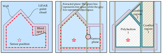
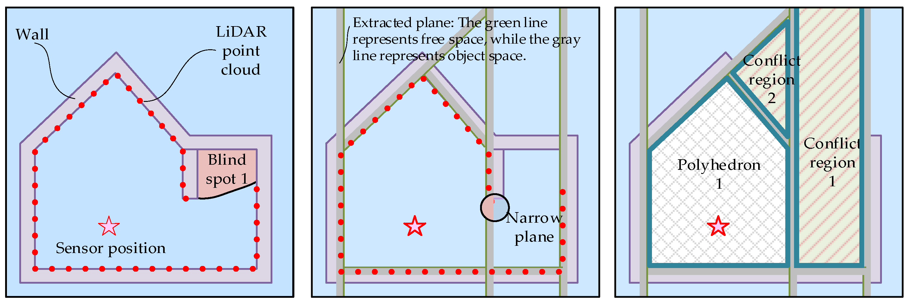
Applying end-to-end modeling training methods to architectural geometric reconstruction can effectively enhance the scalability of the algorithm and reduce system complexity. Chen Z [14], based on plane extraction, performed binary space segmentation and further proposed PolyGNN [15], which divides the space into convex polyhedra based on the extracted planes. The relationships between the convex polyhedra are predicted using a graph neural network to refine the model. This approach simplifies the algorithm design with an end-to-end strategy, offering certain advantages in building exterior reconstruction. In complex indoor scenes or when scan data are incomplete, plane segmentation or space partitioning methods are easily affected by occlusions, blind spots, and locally missing point clouds. As shown in Figure 1, the sensor can only observe partial structures, leaving unobserved regions near openings, corners, and narrow areas, which may cause geometric conflicts among planes, key lines, and polyhedral regions.

Figure 1. Convex polyhedron-based space partitioning is prone to errors in incomplete scans.

3. Methods

3.1. Design of Processing Framework

The incremental geometric reconstruction method proposed in this paper is centered around constructing an automated reconstruction mechanism capable of adapting to complex building structures, automatically repairing scan gaps, and incrementally updating the geometric reconstruction results. The method simplifies the complex 3D spatial analysis problem by applying orthogonal projection to the geometric coordinates, converting it into a simplified 2D plane analysis problem, thereby reducing computational complexity and enabling the fine extraction of geometric features.

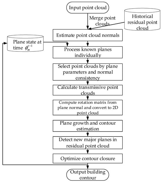
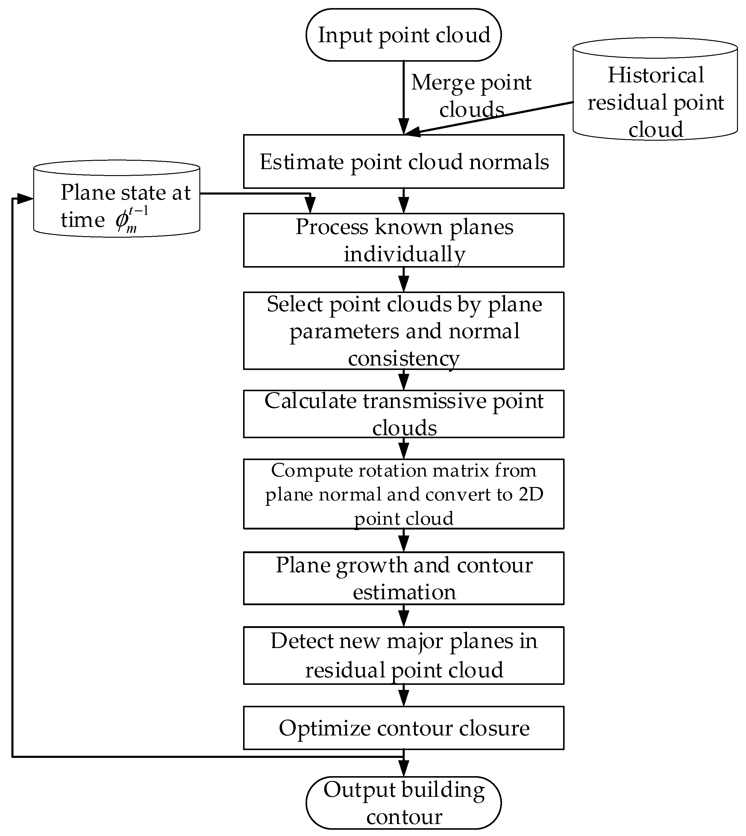
The overall processing framework designed in this paper is shown in Figure 2. The input coordinates of any point are denoted as $x_i=\left(x_i,y_i,z_i\right)\in {ℝ}^3$, the radar position during data collection is $u_i\in {ℝ}^3$, the point cloud normal vector is $n_i\in {ℝ}^3$, the newly acquired point cloud at time t is $\Delta C_t=\left\{x_i\right\}$, and the residual unused point cloud is ${\overline{C}}_{t-1}$. The input points are merged with the residual unused point clouds, and then each known plane is processed individually. Next, the point cloud is selected based on the consistency of the parameters and normal vectors of the known planes, followed by the calculation of transmissive point clouds. The rotation matrix is computed based on the plane’s normal vector, and orthogonal projection is applied to convert it into a 2D point cloud. Plane growth and contour estimation are performed in the 2D space. Finally, unclosed contours are optimized to produce the building’s contour output.

Figure 2. Processing framework.

3.2. Main Plane Detection Algorithm

Horizontal and vertical planes in building structures exhibit different characteristics in terms of point cloud observations and geometric representation. Vertical wall planes usually have stable structural directions. Their bottom edges are generally parallel to the floor, while their side edges are aligned with the gravity direction. Therefore, in the top-down projection, wall structures can often be represented as rectangles or combinations of orthogonal rectangles composed of horizontal and vertical line segments. Based on this property, wall planes can be detected from line features in the 2D projection and further used for subsequent contour growth and opening recovery.

In contrast, although floors and ceilings usually have regular boundaries in complete building structures, their visible regions during incremental scanning are often affected by the limited field of view of the sensor, occlusions, and incomplete local observations. As a result, the dominant orientation and complete boundary of a horizontal plane cannot always be robustly determined from the current point cloud. Therefore, horizontal and vertical planes are detected and estimated separately in this study: vertical planes are mainly constrained by line structures in the top-down projection, while horizontal planes are estimated and updated based on their own observations and their spatial relationships with wall structures.

3.2.1. Horizontal Plane Detection

Horizontal plane detection is a fundamental step in indoor scene geometric reconstruction. Its core task is to accurately identify horizontal structures such as floors and ceilings from cluttered point cloud data. The floor is typically located in the lowest region of the point cloud’s height distribution, the ceiling is in the highest region, and any intermediate horizontal planes usually correspond to floor partitions or large platforms. Based on this common knowledge, this paper proposes a horizontal plane recognition algorithm based on statistical analysis and pulse detection.

Point clouds collected from the same horizontal plane have essentially the same height value, Z, while the Z values of other point clouds are more dispersed. Therefore, an equal-width bin histogram can be used to statistically analyze the Z-value distribution of the point cloud. The pulse peak area of the histogram corresponds to the horizontal plane. The frequency of the i-th histogram bin is represented as:

$$f_i={\displaystyle \sum _{x_j\in C}\mathbb{I}}\left(z_j\in {\mathrm{bin}}_i\right)$$

(1)

where $\mathbb{I}$ is the indicator function, ${\mathrm{bin}}_i=\left[z_{\min }+i\cdot \delta ,z_{\min }+(i+1)\cdot \delta \right)$ is the i-th histogram bin, and $\delta$ is the width parameter of the bin.

To effectively filter out point clouds from other objects and non-structural planes, this paper proposes a pulse detection algorithm based on amplitude and width discrimination for extracting the plane height intervals. A sliding window with width $2N_{\delta }+1$ is used to detect the histogram. If the frequency at the center of the sliding window, f_i, is the maximum frequency within the window, the amplitude and width of the peak pulse are further determined. The width of the peak pulse, w_i, is:

$$w_i=\left\{\begin{array}{ll}{j}_i^{\max }-j_i^{\min }\hfill & \mathrm{if}{f}_i={\displaystyle \underset{j=i-N_{\delta }}{\overset{i+N_{\delta }}{\max }}}(f_j)\hfill \\ 0\hfill & \mathrm{else}\hfill \end{array}\right.$$

(2)

where $j_i^{\min }=\underset{\begin{array}{l}i-N_{\delta }\le j\le i+N_{\delta }\\ f_j\ge k_w\cdot f_i\end{array}}{\arg \min }(f_j)$ and $j_i^{\max }=\underset{\begin{array}{l}i-N_{\delta }\le j\le i+N_{\delta }\\ f_j\ge k_w\cdot f_i\end{array}}{\arg \max }(f_j)$ are the left and right boundaries of the pulse, and $k_w$ is the pulse intensity coefficient parameter.

Furthermore, the pulse is identified as a valid pulse based on the ratio of pulse width and amplitude, and the boundary information of the valid pulse is output, as shown in Equation (3):

$$\overleftrightarrow{z}=\left\{\left.[j_i^{\min },j_i^{\max }]\right|0<w_i<{\omega }_w,\underset{\begin{array}{l}j\in [i-\delta ,i+\delta ]\\ j\notin [j_i^{\min },j_i^{\max }]\end{array}}{\max }(f_j)<2k_p{f}_i\right\}$$

(3)

where ${\omega }_w$ represents the maximum threshold for the width of the valid pulse, and $k_p$ is the threshold for the ratio of the amplitude of the non-valid pulse region within the sliding window to the amplitude of the peak pulse. In this paper, $\delta =40 \mathrm{mm}$, $N_{\delta }=20$, $k_w=0.3$, $k_p=0.1$, and ${\omega }_w=6$.

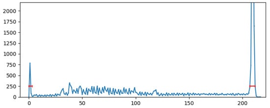
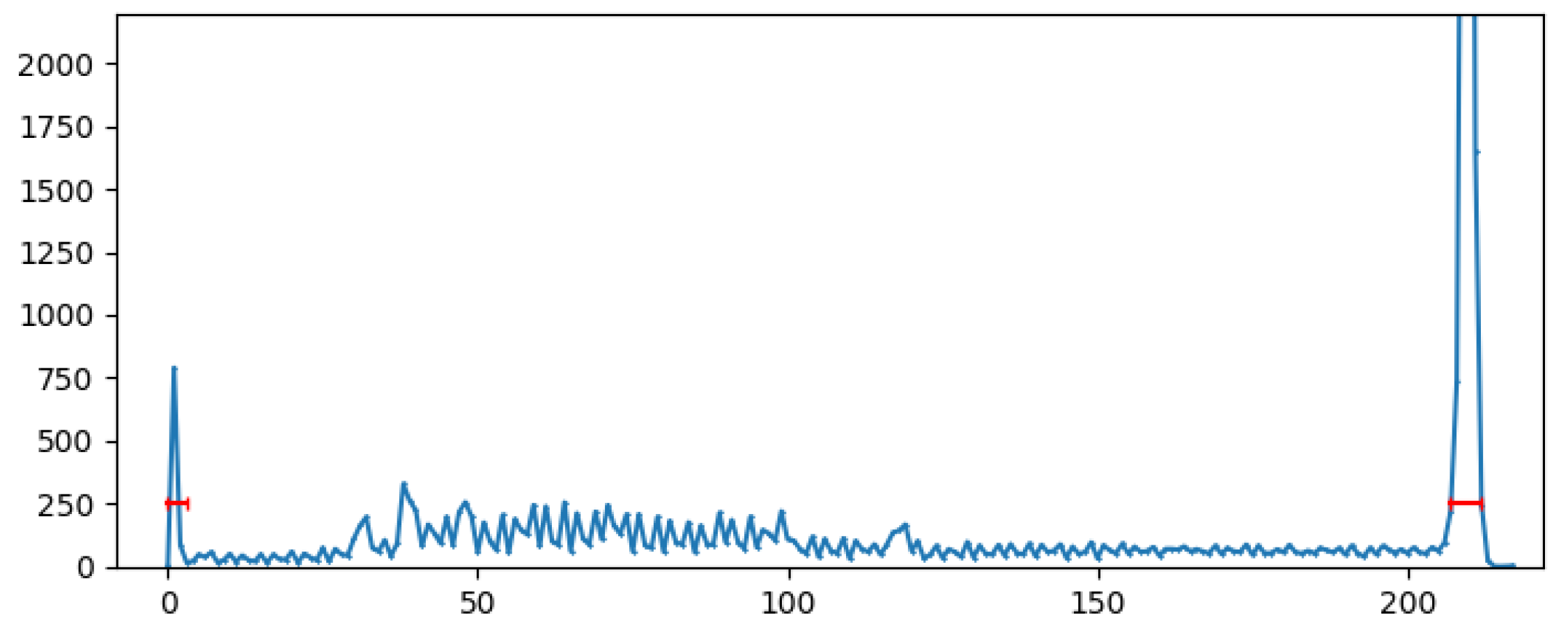
Based on the valid pulse intervals, the corresponding Z-axis range for the horizontal plane is obtained, as shown in Figure 3. The corresponding point cloud data is then extracted, allowing further horizontal plane contour estimation.

Figure 3. Z-axis extraction result of horizontal plane.

3.2.2. Vertical Plane Detection

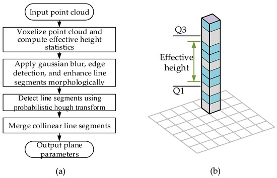
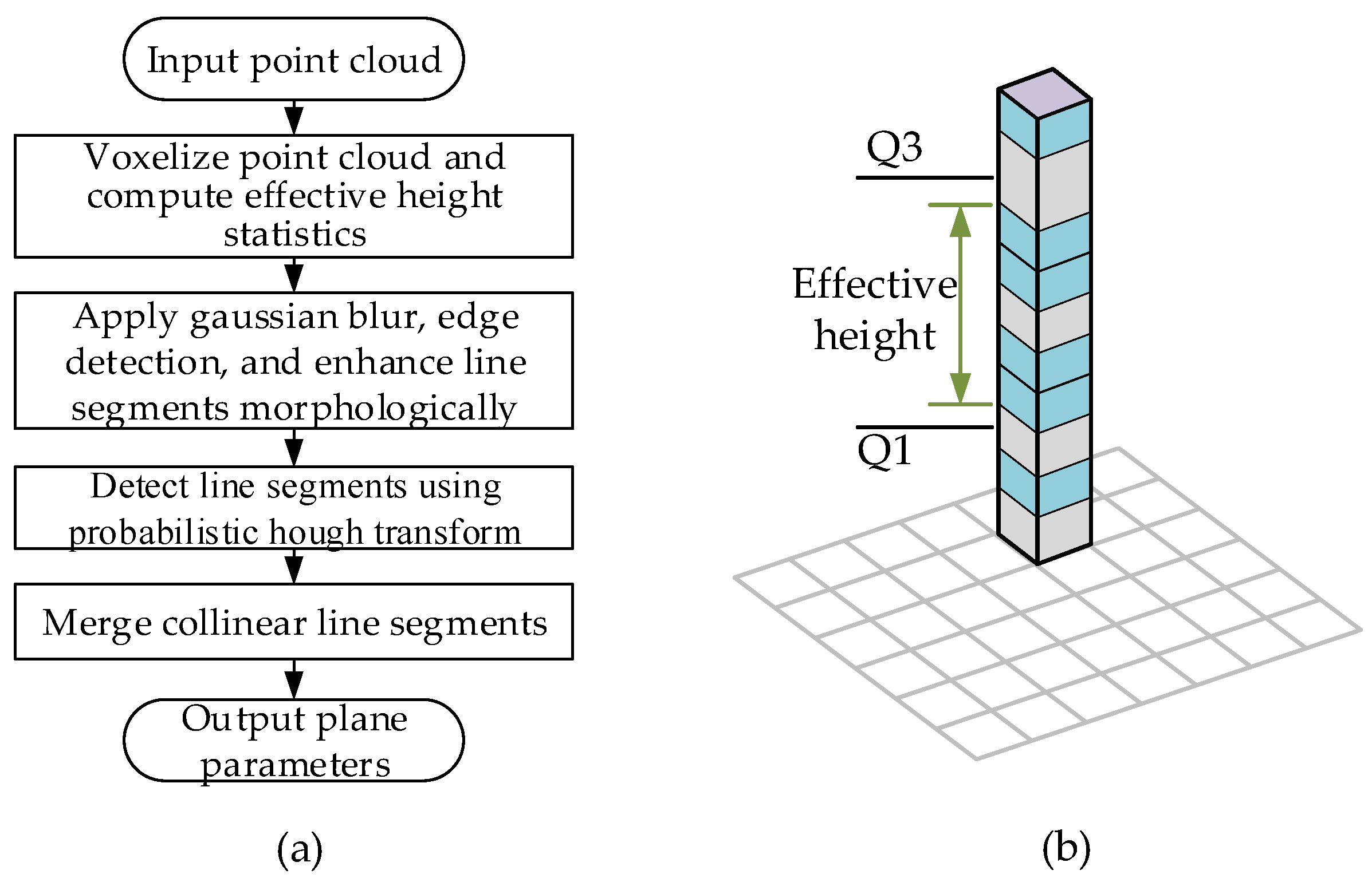
Vertical plane detection, as a key step in indoor scene geometric reconstruction, focuses on accurately extracting vertical structures such as walls, doors and window frames from 3D point cloud data. The vertical planes of the building’s main structure exhibit significant Z-axis height and, in the top-down 2D projection, should appear as narrow line segments. To achieve rapid vertical plane detection, this paper employs a top-down projection and image line segment detection mechanism for plane parameter extraction. The algorithm flowchart is shown in Figure 4a.

Figure 4. Vertical plane parameter extraction algorithm. (a) Vertical plane parameter extraction flowchart. (b) Voxel grid effective height statistics diagram.

To evaluate the effective height of each grid region, this paper uses voxel grid partitioning to divide the space. It then collects the Z-values of the point clouds corresponding to each (X-Y) grid and applies the Interquartile Range (IQR) statistical method to calculate the Z-value range between the first and third quartiles of this set, which is defined as the effective height of the grid region, as shown in Figure 4b. This method enables the conversion of point clouds into a 2D height map.

Due to the limited density of laser point clouds within a short period, local occlusions, noise, and other factors, the line segment characteristics in the 2D height map may not be significant. To address this, the paper sequentially applies Gaussian blur, edge detection, and morphological line segment enhancement to obtain the enhanced contour map. Then, the Probabilistic Hough Transform is used to obtain the line segment parameters. To avoid abnormal segmentation caused by occlusions or other factors, the line segments are further merged based on their collinearity and spacing. The parameters of the extracted plane m can be mapped, ${\phi }_m=\left(n_m,p_m\right)$, where $n_m$ and $p_m$ represent the unit normal vector and a point on the plane m, respectively.

3.3. Plane Contour Detection and Growth Mechanism

Compared to the processing of discrete 3D point clouds, the processing techniques for 2D images are more mature, with a rich library of algorithms available and lower computational complexity. In this section, the plane parameters obtained in Section 3.2 are used for point cloud selection and extraction. The points are projected onto the X-Y plane and then rasterized with a grid resolution of $r=40$ mm. Contour detection is performed based on the rasterized 2D image.

3.3.1. Plane Point Cloud Growth Based on Gradient Analysis

In building scenarios, the floor, ceiling, and walls may have large areas. Due to factors such as construction techniques and cumulative errors in LiDAR measurements, the point clouds belonging to the same plane but different regions may exhibit significant vertical discrepancies. When using a threshold segmentation method for point cloud merging, a small threshold may incorrectly divide point clouds from different regions of the same plane into separate planes, while a large threshold may incorrectly assign point clouds from different structural planes to the same plane. To address this issue, this paper proposes a gradient-based point cloud growth method. For any existing plane ${\varphi }_m^t$, its corresponding point cloud $C_m^t$ and its candidate point cloud $\Delta C_t$ are projected onto the ${\phi }_m$ and rasterized into 2D images $I^c$ and $I^{\Delta }$. From any grid $(i,j)$ containing point clouds, a point $x_k$ is randomly sampled, and the directed distance $d_k$ of this point in the normal vector direction to the plane is calculated. The corresponding pixel value is:

$$I_{ij}=\left\{\begin{array}{ll}{d}_k+\xi \hfill & Whenpointcloudsexistinthegrid\hfill \\ 0\hfill & else\hfill \end{array}\right.$$

(4)

The addition of a positive real number $\xi$ helps differentiate pixels without point clouds from those with a distance of zero, facilitating subsequent processing. The main steps are as follows:

Step 1: Grid image preprocessing: Due to the limited number of LiDAR points collected within a short period, the obtained grid images $I^c$ and $I^{\Delta }$ may have many missing pixels. To obtain effective boundary information, the images are sequentially processed with closing operations to reduce the interference caused by missing pixels.

Step 2: For the newly added point clouds, the image is segmented into regions using pixel gradients, where gradients greater than the threshold are considered boundary points, causing a fracture between the regions on either side of the boundary. These regions are then updated as $I^{\Delta \prime }$.

Step 3: Plane corresponding point cloud growth. For the plane grid image $I^c$ and $I^{\Delta \prime }$, calculate the connected regions. For the regions where there is an intersection between $I^{\Delta \prime }$ and $I^c$, the corresponding point clouds are assigned to the current plane, achieving the growth of the plane point cloud.

3.3.2. Hole Point Cloud Generation Based on Transmissive Relationships

Common reconstruction algorithms estimate object contours and holes based on the acquired point clouds. However, in efficient reconstruction applications, the radar’s sampling angles are limited over short periods, leading to a restricted view of the generated point clouds. As a result, contour estimation based on actual point clouds often results in numerous erroneous hole structures. To achieve more reliable, efficient geometric reconstruction, this paper proposes a hole detection strategy based on transmissive relationships.

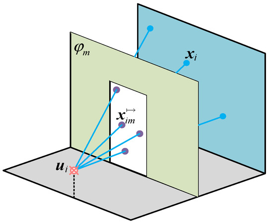
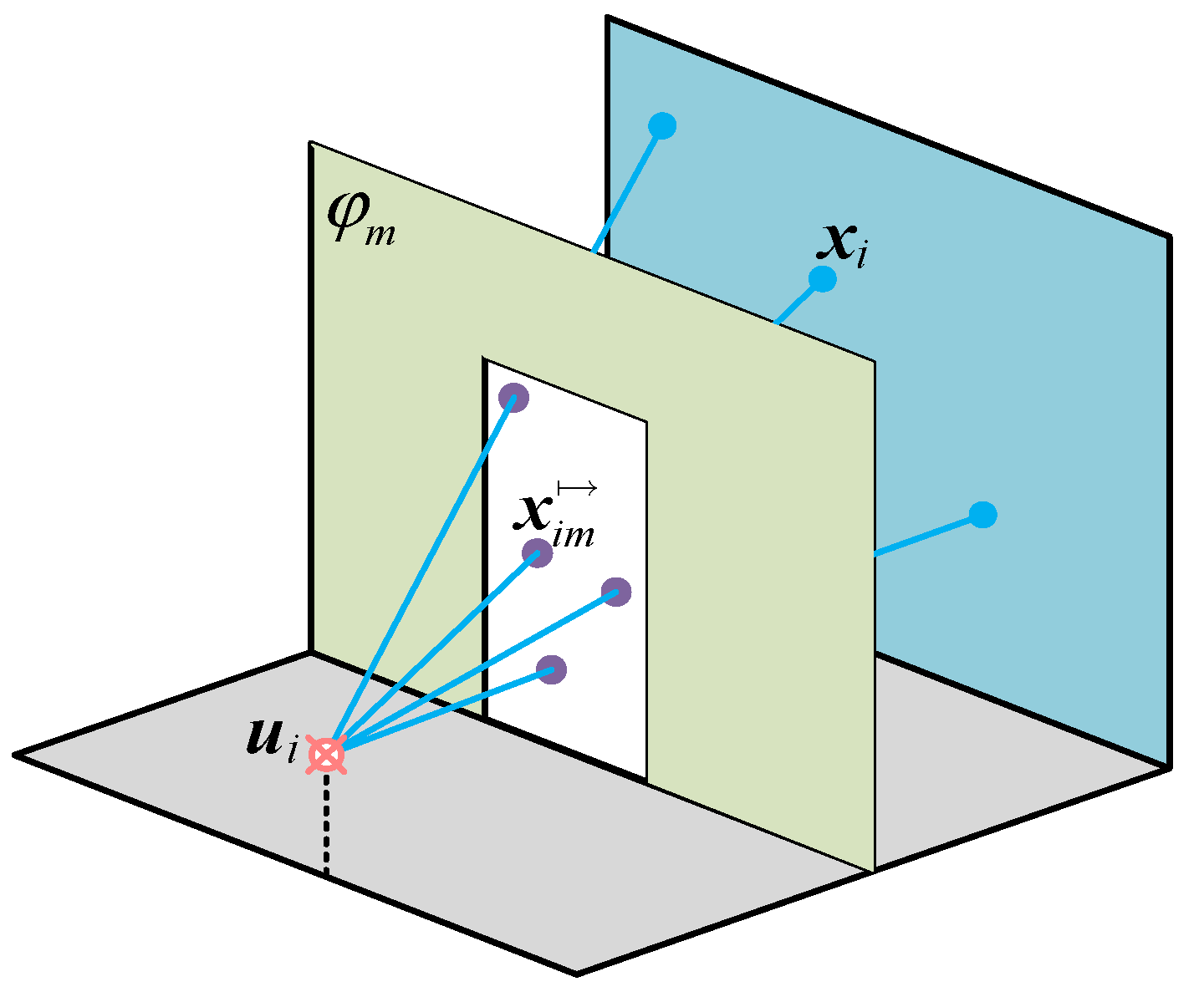
The point cloud’s transmissive effect through the plane hole structure is shown in Figure 5. From position $u_i$, the point cloud set $\Delta C_t$ is measured. The point cloud set $\Delta {\cancel{C}}_m^t$, which is transmitted through the hole structure of the plane ${\phi }_m$, can be represented as:

$$\Delta {\cancel{C}}_m^t=\left\{\left.x_{im}^{\mapsto }\right|d_{im}^u{d}_{im}^x<0,\left|d_{im}^x\right|>\varsigma ,x_i\in \Delta C_t\right\}$$

(5)

where $x_{im}^{\mapsto }=u_i+{\displaystyle \frac{\left|d_{im}^u\right|}{\left|d_{im}^x\right|+\left|d_{im}^u\right|}}(x_i-u_i)$ is the transmitted position of the measurement point $x_i$ on the plane ${\phi }_m$, $d_{im}^u=\left(u_i-p_m\right)\cdot n_m$ and $d_{im}^x=\left(x_i-p_m\right)\cdot n_m$ represent the distances from the LiDAR and the laser measurement point $x_i$ to the plane ${\phi }_m$, respectively.

Figure 5. Generation of hole point cloud based on transmission relationship.

3.3.3. Geometry Contour Estimation Based on Transmissive Expansion

To achieve continuous, consistent, and stable plane contour reconstruction, the state data of each plane is recorded as:

$${\varphi }_m^t=\left\{n_m^t,p_m^t,C_m^t,{\cancel{C}}_m^t,{▱}_m^t,{\cancel{▱}}_m^t\right\}$$

(6)

where $C_m^t={\displaystyle {\cup }_{\tau \le t}\Delta C_m^{\tau }}$ and ${\cancel{C}}_m^t={\displaystyle {\cup }_{\tau \le t}\Delta {\cancel{C}}_m^{\tau }}$ represent the point cloud at time t that supports the plane contour estimation and the transmitted point cloud supporting the hole contour estimation, respectively. ${▱}_m^t$ and ${\cancel{▱}}_m^t$ represent the outer plane contour and hole contour estimated at time t, respectively. The newly added supporting point cloud $\Delta C_m^t$ at time t is represented as:

$$\Delta C_m^t=\left\{x_i\left|\left|d_{im}^x\right|<{\delta }_d,n_x\cdot n_i>{\delta }_{\theta },x_i\in C_t\right.\right\}$$

(7)

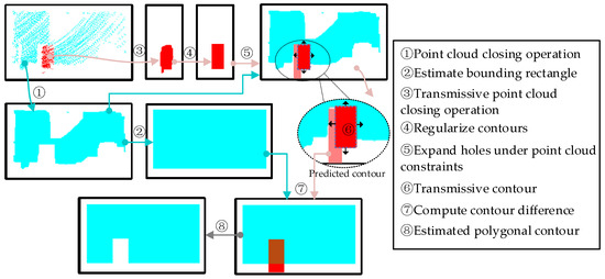
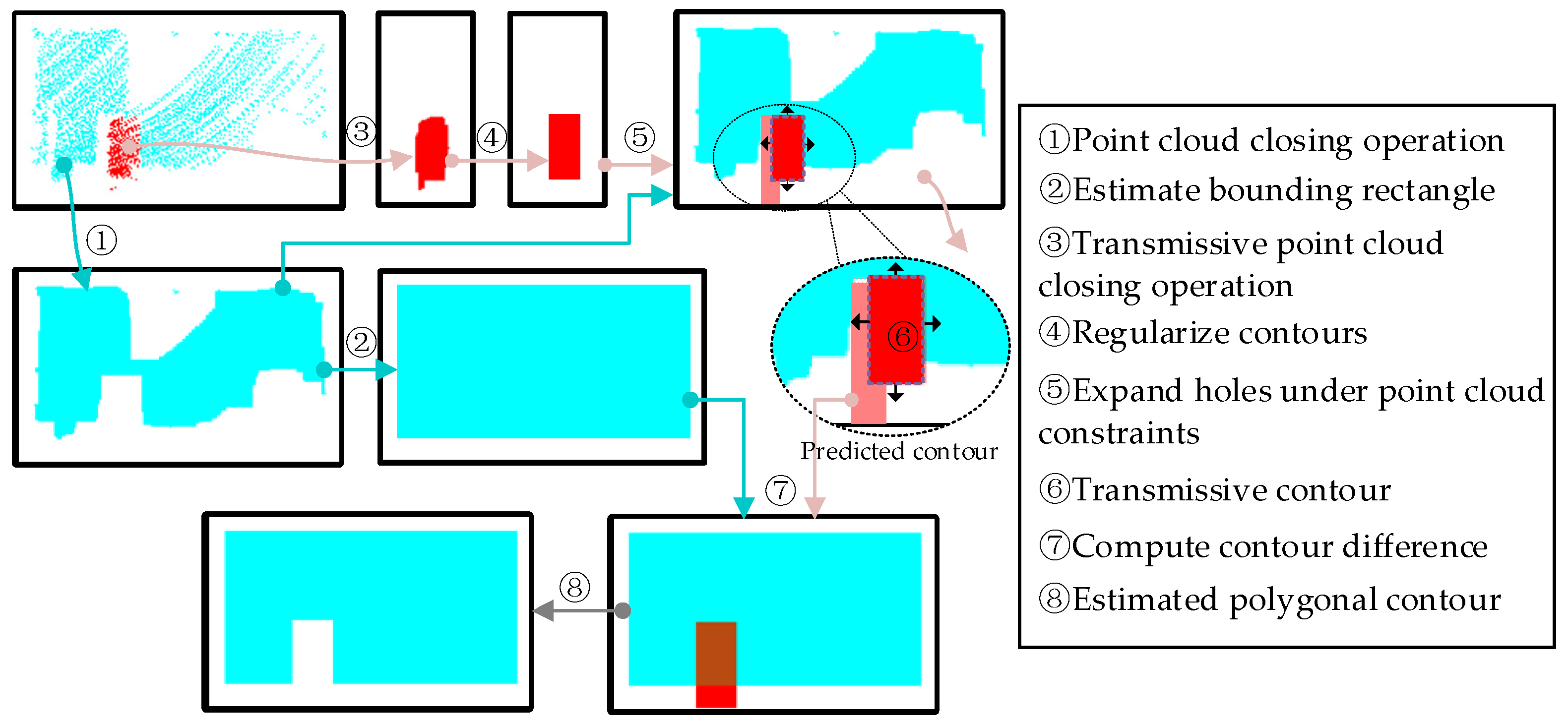
Due to the limited sampling rate of LiDAR and the specific scanning strategy, certain areas of the plane may not be scanned or may have low density during short-time scans. To obtain a complete and concise plane contour and avoid incorrectly identifying unscanned areas as hole structures, it is necessary to estimate and predict based on the acquired supporting point cloud and transmitted point cloud. The algorithm logic is shown in Figure 6:

Figure 6. Schematic of geometry contour estimation based on transmissive expansion.

Step 1: The point cloud is rasterized, and the image undergoes a closing operation. Since the point cloud is sparse within a short time, the closing operation is applied first to fill the gaps between point clouds while ensuring the consistency of the contour. The closed contour is used both to support the estimation of the plane and for the estimation of hole contours.

Step 2: Bounding rectangle estimation for plane contours. To avoid incorrectly identifying unsampled areas as hole structures, a bounding rectangle is used as the predicted outer contour of the plane.

Step 3: Hole structure regularization. A closing operation is first applied to the transmissive point cloud in the same manner as Step 1. The hole structures are then regularized by representing them with simplified orthogonal polygons and removing local noisy point clouds.

Step 4: Hole expansion under point cloud constraints. The algorithm only identifies a region as a hole when there are transmitted point clouds. However, due to occlusion or incomplete coverage of the view angle, both transmitted and supporting point clouds cannot independently and accurately estimate the hole contour. Therefore, hole expansion under point cloud constraints is used to estimate the hole structure. The orthogonal polygon of the hole estimated in Step 3 is expanded outward along the orthogonal direction until it intersects with the supporting point cloud, at which point the expansion stops.

Step 5: Difference between the bounding rectangle of the plane contour and the estimated transmitted contour. The transmissive contour is first obtained from the regularized hole polygons. Then, by computing the difference between the transmissive contour and the main plane, undetected areas are filled in while preserving the hole structure as accurately as possible. The resulting polygonal contour serves as the estimated plane boundary.

3.4. Contour Closure

Due to noise during the LiDAR point cloud acquisition process and the accuracy limitations of rasterization for plane contour extraction, gaps or interference may occur between the reconstructed planes. To address this, this paper corrects the contours based on the orthogonal projection relationship between the planes, enhancing the reconstruction results.

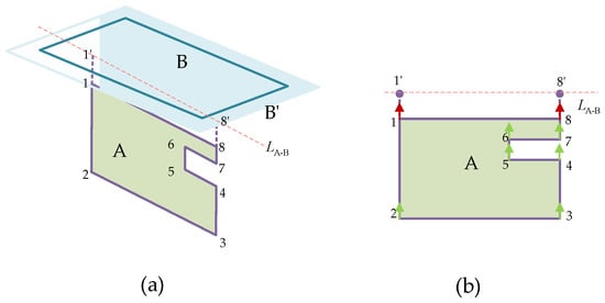
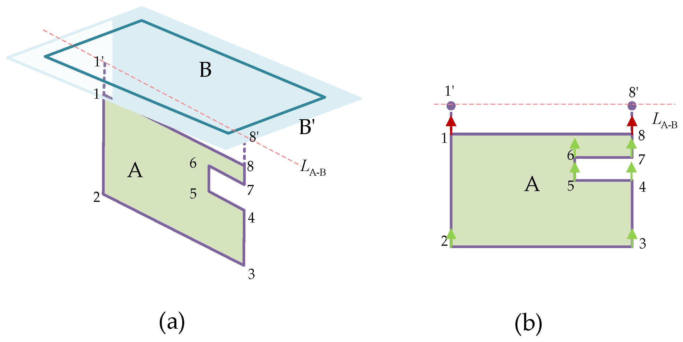
The contour closure logic between planes is shown in Figure 7a. For any plane A to be closed, the first step is to select candidate reference planes based on the orthogonal relationship between planes. When using plane B as a reference, the outer-expanded equidistant polygon B’ of plane B is obtained, and the intersection line $L_{\mathrm{A}\text{-}\mathrm{B}}$ between planes A and B is calculated. From the vertices of the polygon within plane A, those vertices whose distance to the intersection line is smaller than the threshold ${\delta }_{\mathrm{A}\text{-}\mathrm{B}}$, whose adjustment direction does not interfere with the polygon itself, and whose projection points lie inside contour B’ are selected. These vertices are then adjusted to the intersection line projection points, thereby achieving contour closure between the planes, as shown in Figure 7b.

Figure 7. Schematic of contour closure between planes. (a) Perform inter-plane contour closure correction. (b) Select points for effective closure adjustment.

4. Results

4.1. Simulation Experiment and Quantitative Results

To further verify the performance of the proposed method under controlled conditions, simulation experiments were first conducted. The simulation scene was constructed in the NVIDIA Isaac Sim platform [16] and contains typical building structures such as walls and openings. Specifically, the scene is divided into two separate rooms by an internal partition wall, and each room is connected to the exterior through a large rectangular opening. The overall structure resembles an industrial-style container or temporary prefabricated building. Since complete geometric ground truth is available in the simulation environment, it provides a reliable basis for quantitatively evaluating the reconstruction accuracy and structural completeness of the proposed method. All experiments were performed on a workstation with a 13th Gen Intel Core i7-13700K CPU, 32 GB RAM, and Ubuntu 22.04 operating system.

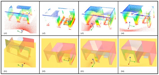
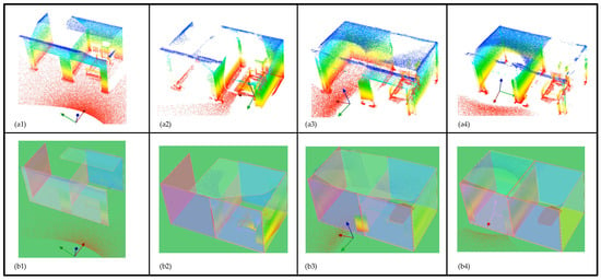
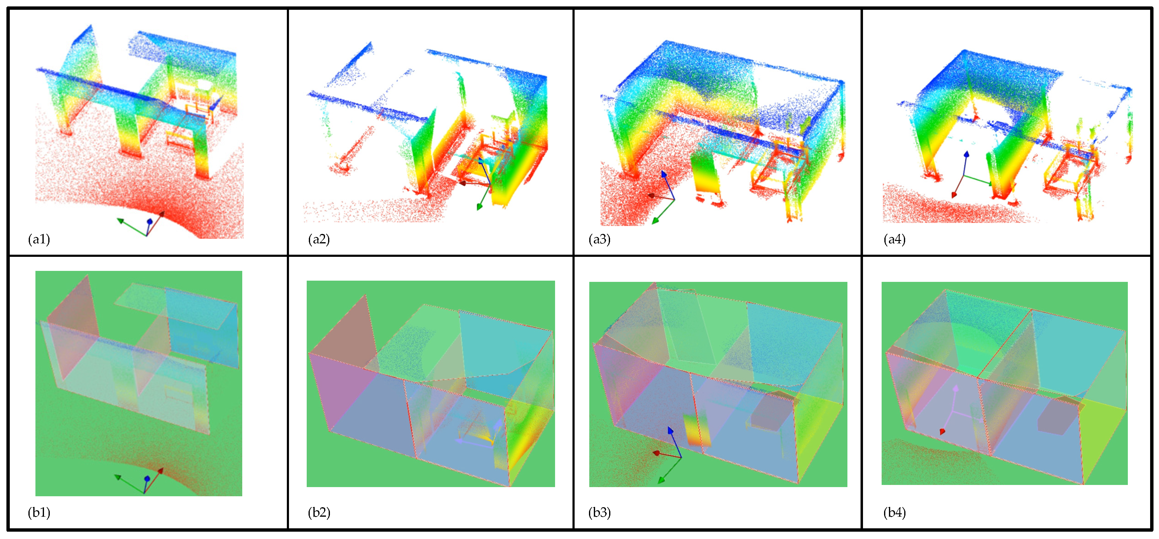
Based on this scene, the proposed reconstruction method was applied, and the reconstruction process was visualized. As shown in Figure 8, the coordinate axes indicate the position and pose of the LiDAR at different time steps, and the input point clouds only provide local observations from the corresponding viewpoints. With the progressive input of point cloud data, the method gradually performs dominant plane detection, contour growth, and hole detection, and finally reconstructs a relatively complete structural contour of the scene. The results indicate that the proposed method can stably recover the major structural boundaries and maintain good contour continuity and structural consistency even in the presence of local missing regions.

Figure 8. Progressive reconstruction process in the simulation scene.

Figure 8(a1–a4) show the point cloud inputs at four different time points, while Figure 8(b1–b4) present the corresponding incremental reconstruction results. As the LiDAR pose changes, each input point cloud captures only a partial observation of the scene. Nevertheless, the constructed planes are continuously updated and refined, and openings such as doors and windows are preserved through the transmissive relationship rather than being incorrectly filled as missing regions.

For quantitative evaluation, points were uniformly sampled inside each reconstructed contour with an interval of 0.10 m, and the ground-truth contours were sampled in the same manner. Based on the nearest-neighbor distances between the reconstructed point set and the ground-truth point set, Chamfer Distance L1 (CD-L1), Chamfer Distance L2 (CD-L2), precision, recall, and F1-score were computed [17]. The distance threshold for precision, recall, and F1-score was set to 0.10 m.

As shown in Table 1, the proposed method achieves favorable quantitative performance in the simulation scene. Specifically, the CD-L1 and CD-L2 values are 0.088 m and 0.007 m², respectively, indicating a small overall geometric deviation from the ground truth. The completeness L1 and accuracy L1 are 0.049 m and 0.039 m, showing that the method performs well in both structural completeness and local reconstruction accuracy. In addition, under the 10 cm threshold, the precision and recall reach 85.1% and 95.6%, respectively, yielding an F1-score of 0.901. These results demonstrate that the proposed method can recover building structure contours with both high completeness and good geometric accuracy. To further evaluate the processing efficiency of the proposed method on the simulation data, five repeated tests were conducted on the point-cloud frame processing procedure in the simulation scene. Each point-cloud frame contains approximately 100,000 points. We repeated the full simulation experiment five times. Across the five tests, the mean of the per-test average frame-processing times was 1.04 s, with the per-test averages ranging from 0.97 s to 1.05 s and a standard deviation of 0.03 s. For instance, in one representative 56-frame test, the per-frame time averaged 1.02 s, with a minimum of 0.61 s and a maximum of 1.67 s. Since each point-cloud frame corresponds to approximately 1 s of LiDAR data acquisition in this experimental setting, the result indicates that the proposed method can complete incremental structural updating at a rate close to the data acquisition interval in the simulation scene. All runtime measurements exclude visualization, data loading, result saving, and waiting time.

Table 1. Quantitative evaluation of reconstruction results in the simulation scene.

Metric	Value
CD-L1	0.088 m
CD-L2	0.007 m2
Precision @10 cm	85.1%
Recall @10 cm	95.6%
F1-score @10 cm	0.901
Average processing time	1.02 s

To further evaluate the influence of reduced point-cloud density on the transmissive relationship-based hole detection strategy, a downsampling robustness test was conducted on the simulation data. Since the simulation scene contains two main door openings, the horizontal offset of the detected opening contour relative to the ground-truth opening contour was used to evaluate the stability of opening detection. The sampling rates were set to 90%, 80%, and 70%. The downsampled point clouds were processed using the same reconstruction pipeline.

The results show that when the sampling rate was reduced to 90%, almost no horizontal offset was observed for either opening. When the sampling rate was reduced to 80%, the horizontal offsets of the two openings were approximately 1 mm and 23 mm, respectively. When the sampling rate was further reduced to 70%, the horizontal offsets of the two openings were 13 mm and 39 mm, respectively. These results indicate that both door openings can be successfully detected when the sampling rate is no lower than 70%, and the maximum horizontal offset remains within 4 cm. For building openings such as door frames, this level of deviation is within an acceptable error range. Therefore, in the tested simulation scene, moderate reduction in point-cloud density only has a limited influence on the reconstruction result and does not lead to obvious degradation of the transmissive hole detection capability.

4.2. Ablation Study on Transmissive Hole Detection Strategy

To verify the effectiveness of the transmissive hole detection strategy, an ablation study was further conducted. The proposed method can predict and complete unobserved regions based on the existing plane contours. However, for real openings such as doors and windows, if the hole detection constraint is removed, these regions are treated as ordinary missing areas and are completed as solid polygons. This leads to incorrect filling of opening regions in the reconstructed building structure.

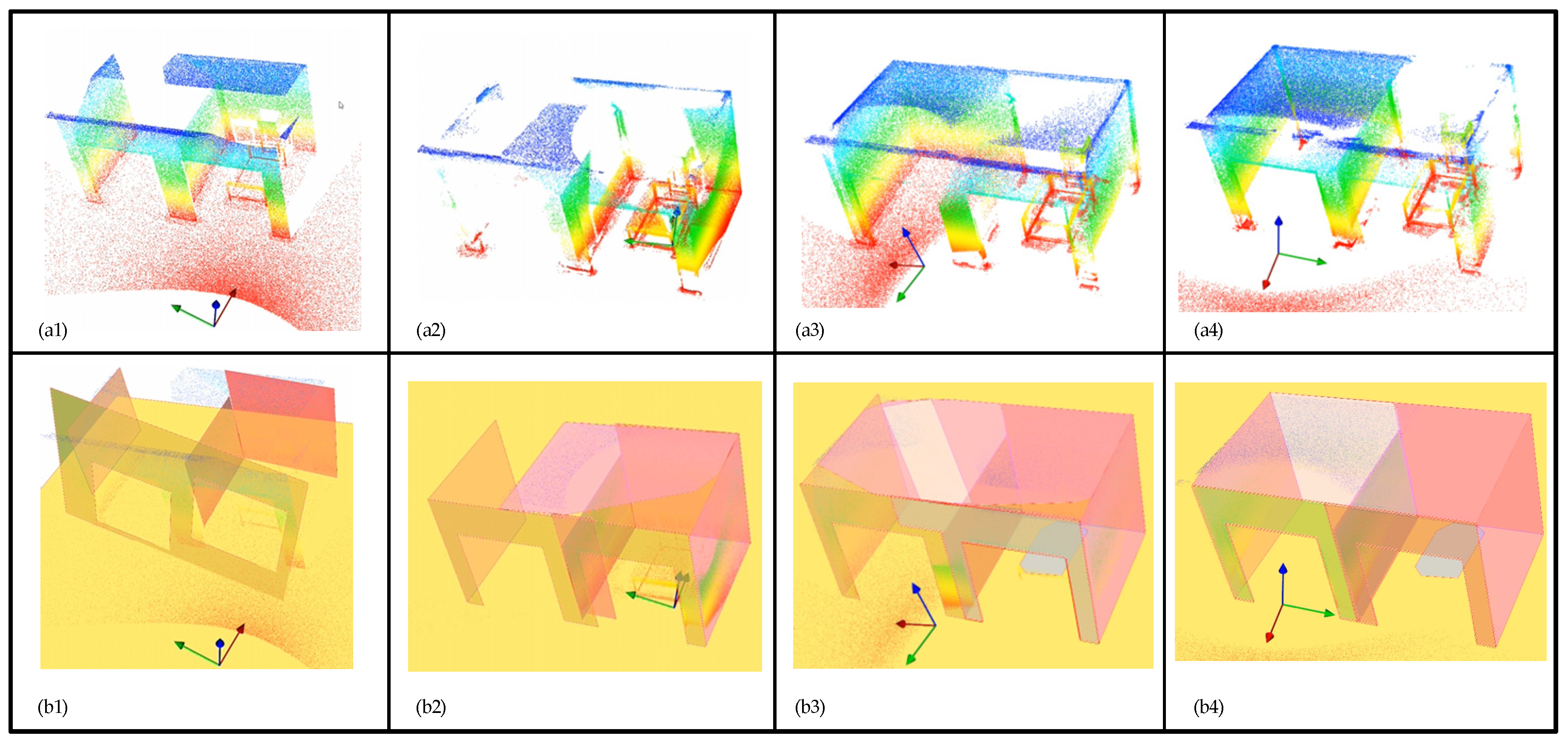
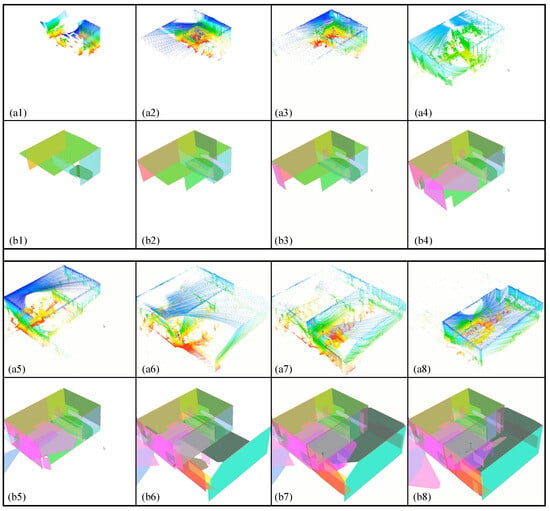
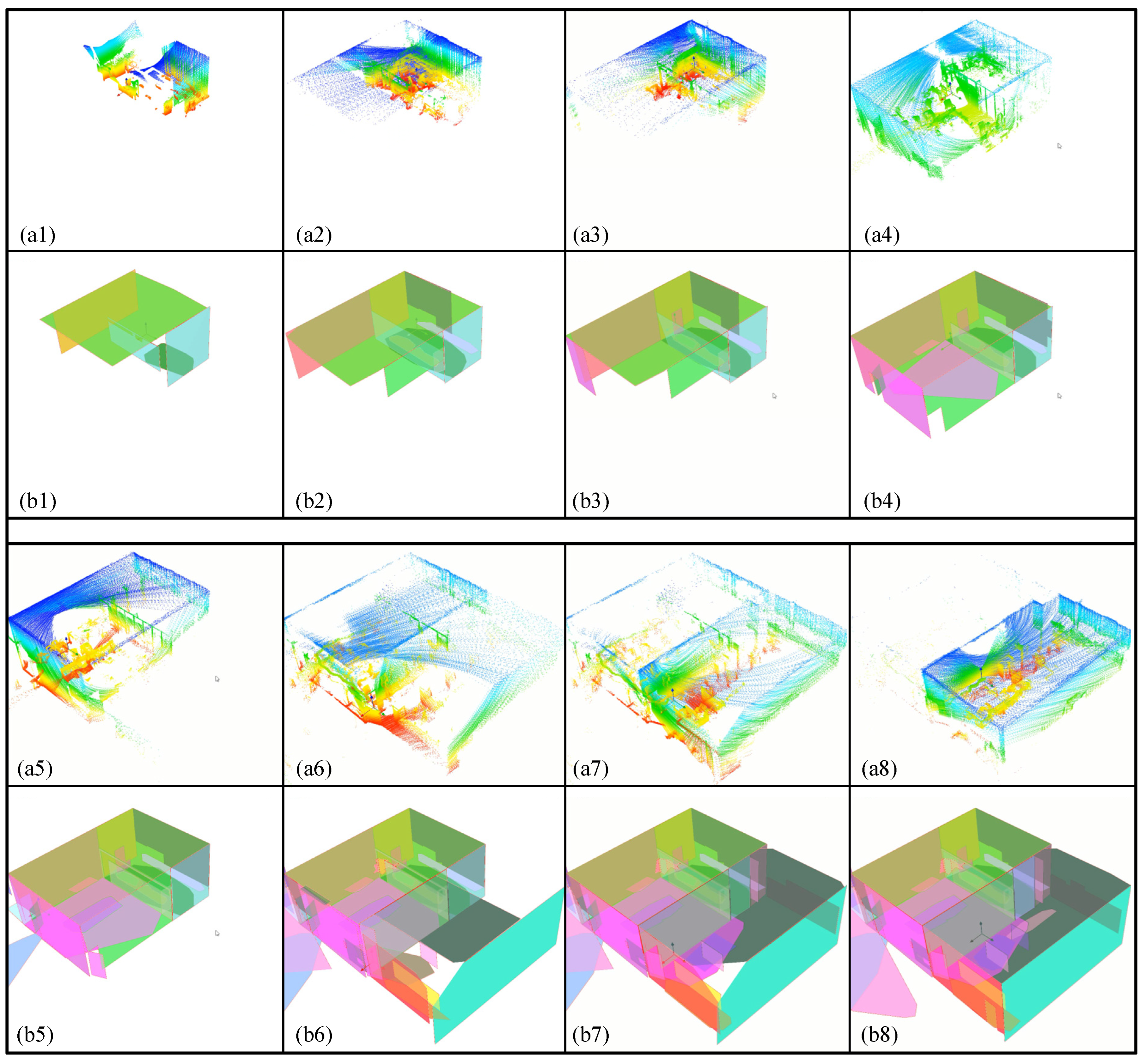
Figure 9 shows the mapping process and final reconstruction result without the transmissive hole detection strategy. Figure 9(a1–a4) show the point cloud inputs at four different time points, while Figure 9(b1–b4) present the corresponding incremental reconstruction results. It can be observed that, without the transmissive constraint, the wall contours can still maintain good continuity, but opening regions such as doors and windows are incorrectly regarded as areas to be completed, resulting in solid wall structures in the reconstruction. In contrast, the complete method uses the transmissive point cloud relationship formed when LiDAR rays pass through openings to identify and recover real hole regions, thereby preventing doors and windows from being incorrectly filled.

Figure 9. Progressive reconstruction process without transmissive hole detection strategy.

To further quantify the contribution of this module, the same evaluation metrics were computed for the reconstruction results without the hole detection strategy and compared with those of the complete method. The results are listed in Table 2. It can be seen that, after removing the hole detection strategy, the overall contours can still be completed, but the geometric discrepancy from the ground truth increases because real openings are filled incorrectly. As a result, metrics such as precision and F1-score decrease. These results demonstrate that the transmissive hole detection strategy can effectively distinguish between unobserved missing regions and real architectural openings, and is therefore a key component for improving the reconstruction accuracy of empty structures such as doors and windows.

Table 2. Quantitative comparison of the ablation study on transmissive hole detection strategy.

Metric	Without Hole Detection	With Hole Detection
CD-L1	0.152 m	0.088 m
CD-L2	0.038 m2	0.007 m2
Precision @10 cm	71.1%	85.1%
Recall @10 cm	96.1%	95.6%
F1-score @10 cm	0.817	0.901
Average processing time	0.92 s	1.02 s

Table 2 presents the quantitative results before and after removing the hole detection strategy. It can be observed that the reconstruction performance degrades significantly when the transmissive hole detection strategy is removed. Specifically, the CD-L1 and CD-L2 values increase from 0.088 m and 0.007 m² to 0.152 m and 0.038 m², respectively, indicating a substantial increase in the overall geometric error. Meanwhile, the precision decreases from 85.1% to 71.1%, and the F1-score decreases from 0.901 to 0.817, showing that more incorrectly reconstructed regions are introduced. In terms of computational time, the average single-frame processing time decreases slightly from 1.02 s to 0.92 s after removing the hole detection strategy. This indicates that the transmissive hole detection module introduces only a limited additional computational cost, while it substantially improves the geometric accuracy and structural correctness of the reconstruction.

It should be noted that the recall slightly increases from 95.6% to 96.1% after removing the hole detection strategy. This is because recall mainly reflects the coverage of the reconstructed result with respect to the ground truth. Without the hole detection constraint, real empty regions such as doors and windows are incorrectly completed as solid structures, which increases the coverage of the reference geometry and leads to an inflated recall value.

Therefore, although the recall slightly increases after removing the hole detection strategy, this increase is caused by incorrect completion and does not indicate better reconstruction quality. Considering the CD, precision, and F1-score metrics, the transmissive hole detection strategy effectively prevents openings such as doors and windows from being incorrectly filled and plays an important role in improving the geometric accuracy and structural consistency of the reconstruction.

4.3. Parameter Sensitivity Analysis

We further evaluate how the reconstruction accuracy responds to variations in key parameters in the proposed method. We select three parameters for this analysis: the grid resolution $r$ (default 40 mm), the pulse intensity coefficient $k_w$ (default 0.3), and the contour closure threshold $\delta$ (default 400 mm). These three parameters each control a distinct stage of the pipeline: $r$ governs the geometric precision of 3D-to-2D projection and contour extraction; $k_w$ determines the sensitivity of pulse-based horizontal plane detection, which serves as the reference for subsequent vertical structure inference; and $\delta$ is the sole control variable in the contour closure procedure. Since these parameters operate on independent modules without mutual coupling, the sensitivity of each module to its own perturbation can be assessed separately. Other fixed parameters in the method, such as the contour simplification tolerance epsilon (fixed at 3 pixels) and the point-to-plane distance threshold (fixed at 200 mm), are excluded from this analysis: the former has negligible effect within a 1–2 pixel variation under the 40 mm grid resolution, and the latter is determined by the range error characteristics of the LiDAR sensor rather than being a freely tunable algorithmic parameter.

For each parameter, we test five values while keeping the other two parameters at their defaults. All experiments are conducted on the same simulation scene and under the same evaluation protocol described in Section 4.1. Table 3 summarizes the CD-L1, CD-L2, Precision, Recall, and F1-score for each configuration.

Table 3. Parameter sensitivity analysis. Default values are in bold.

Parameter	Value	CD-L1	CD-L2	Precision @10 cm	Recall @10 cm	F1-Score @10 cm
$r$	20	0.083 m	0.007 m2	85.0%	95.6%	0.901
	30	0.083 m	0.007 m2	84.2%	95.6%	0.896
	40	0.088 m	0.007 m2	85.1%	95.6%	0.901
	50	0.081 m	0.006 m2	85.6%	96.0%	0.909
	60	0.126 m	0.049 m2	83.0%	93.6%	0.883
$k_w$	0.1	0.083 m	0.006 m2	85.5%	96.0%	0.907
	0.2	0.124 m	0.049 m2	84.1%	93.6%	0.888
	0.3	0.088 m	0.007 m2	85.1%	95.6%	0.901
	0.5	0.085 m	0.007 m2	85.1%	95.1%	0.901
	0.7	0.088 m	0.008 m2	82.3%	96.0%	0.891
$\delta$	200	0.082 m	0.007 m2	85.4%	95.3%	0.903
	300	0.082 m	0.006 m2	85.6%	95.8%	0.907
	400	0.088 m	0.007 m2	85.1%	95.6%	0.901
	500	0.094 m	0.008 m2	83.2%	96.0%	0.889
	600	0.082 m	0.006 m2	85.2%	96.0%	0.906

Grid resolution $r$. We first examine the grid resolution used in the 2D projection stage. As shown in Table 4, the F1-score remains above 0.883 for $r$ from 20 mm to 50 mm, and CD-L1 stays around 0.081–0.088m. This indicates that the contour extraction module is largely insensitive to the choice of grid resolution within this range. At $r=60$ mm, however, both CD-L1 and F1-score degrade noticeably (0.126 m and 0.883, respectively). The reason is that a coarser grid smooths out the fine geometry near openings such as doors and windows: the effective pixel count of small holes falls below the detection threshold of 0.1 m², and the morphological dilation–erosion operations in the contour estimation step erase thin structural boundaries. The default value $r=40$ mm lies within the stable range and provides a reasonable balance between geometric accuracy and computational cost.

Table 4. Quantitative comparison with classical reconstruction methods.

	Proposed	Poisson Reconstruction	BPA
CD-L1	0.088 m	0.092 m	0.097 m
CD-L2	0.007 m2	0.008 m2	0.009 m2
Precision @10 cm	85.1%	80.7%	79.9%
Recall @10 cm	95.6%	99.9%	99.9%
F1-score @10 cm	0.901	0.893	0.888
Normalized processing time	1.02 s	0.35 s	19.58 s

Pulse intensity coefficient $k_w$. We then analyze $k_w$, which controls how strictly the pulse detection algorithm isolates horizontal planes from the Z-value histogram. From Table 3, we observe that the method performs robustly across a wide range from $k_w=0.1$ to 0.7, with F1-scores between 0.888 and 0.907, except for an isolated degradation at $k_w=0.2$. At this value, CD-L1 rises from approximately 0.083 m to 0.124 m, and F1 drops to 0.888. The reason is that at this intermediate value, the detected pulse width is partially truncated: Z-value bins near the pulse boundary that should belong to the horizontal plane are excluded, and the resulting incomplete floor or ceiling contour is inherited by the downstream hole detection module. In contrast, $k_w=0.1$ does not exhibit this issue: although the discrimination is looser, the clean point cloud data in the simulation scene produces well-separated Z-value pulses that remain intact even under relaxed criteria.

Contour closure threshold $\delta$. The threshold $\delta$ controls the maximum distance for adjusting vertices toward the intersection line between adjacent planes during contour closure. Table 3 shows that this parameter has the weakest influence among the three: F1-scores vary only between 0.889 and 0.907 across the entire 200–600 mm range, and CD-L1 fluctuates within 0.082–0.094 m. This flat response is expected because the contour closure procedure incorporates additional geometric checks—including projection-in-polygon verification and segment intersection tests—that filter out inappropriate adjustments independent of the distance threshold. The default value $\delta =400$ mm sits near the center of this wide stable range.

Overall. The above results indicate that the reconstruction accuracy of the proposed method remains stable across a wide range of parameter values, with all default settings falling within flat optimal regions. The overall principle guiding parameter selection is to preserve major structural elements such as walls, floors, and ceilings while using appropriate grid granularity and discrimination thresholds to suppress non-structural details caused by point cloud sparsity and partial occlusions. The sensitivity analysis confirms the effectiveness of this parameter configuration strategy: when each module is independently perturbed, the reconstruction accuracy exhibits no sharp fluctuation, demonstrating that the method as a whole possesses favorable parameter robustness.

4.4. Comparison with Classical Reconstruction Methods

After verifying the contribution of the transmissive hole detection strategy through the ablation study, this section further evaluates the proposed method against representative classical reconstruction methods in terms of computational time, processed data volume, reconstruction accuracy, and output representation. Two widely used surface reconstruction methods, Poisson Reconstruction and BPA, were selected for comparison because they generate triangular mesh models directly from point cloud data.

It should be noted that Poisson Reconstruction and BPA differ significantly from the proposed method in terms of processing paradigm. Poisson Reconstruction and BPA typically operate in a batch-processing manner, where the accumulated point cloud is processed globally to generate a complete triangular mesh model. In contrast, the proposed method adopts an incremental frame-by-frame reconstruction strategy, where a fixed number of points, 100,000 points per frame, are processed at each step, and the building structural model is progressively updated using historical plane states. Therefore, although these methods can be compared using the same point-cloud data in terms of accuracy and efficiency, their target applications and reconstruction paradigms are not strictly identical.

To enable a fairer efficiency comparison between the incremental method and the batch-processing methods, the total processing time of each method was normalized by the number of input points and reported as the average time required to process 100,000 points. For the proposed method, 100,000 points correspond to one processing frame. For Poisson Reconstruction and BPA, the value was obtained by dividing the total processing time for the complete input point cloud by the number of input points and then converting it to the time per 100,000 points. All runtime measurements exclude visualization, data loading, result saving, and artificial waiting time.

Table 4 summarizes the comparison results in terms of runtime, reconstruction accuracy, and output representation.

As shown in Table 4, the proposed method achieves favorable geometric accuracy compared with the two classical reconstruction methods. Specifically, the proposed method obtains the lowest CD-L1 and CD-L2 values, 0.088 m and 0.007 m², respectively, indicating a smaller overall geometric deviation from the reference structure. In addition, the precision of the proposed method reaches 85.1%, which is higher than that of Poisson Reconstruction, 80.7%, and BPA, 79.9%. This suggests that the proposed method introduces fewer incorrectly reconstructed regions and produces cleaner structural boundaries.

It should be noted that Poisson Reconstruction and BPA both achieve a higher recall of 99.9%, compared with 95.6% for the proposed method. However, a higher recall mainly reflects the coverage of the reconstructed result with respect to the reference structure and does not necessarily indicate better overall reconstruction quality. When combined with the relatively lower precision, especially for BPA, this result suggests the presence of over-reconstruction, where additional mesh surfaces are generated outside the true structural regions. Therefore, the F1-score provides a more balanced evaluation of reconstruction quality. The proposed method achieves the highest F1-score of 0.901, outperforming Poisson Reconstruction and BPA, which obtain F1-scores of 0.893 and 0.888, respectively.

In terms of computational efficiency, Poisson Reconstruction achieves the shortest normalized processing time, 0.35 s per 100,000 points, indicating high efficiency for single-batch surface reconstruction. The proposed method requires 1.02 s per 100,000 points, which is slower than Poisson Reconstruction but still comparable to the LiDAR acquisition interval of approximately 1 s for 100,000 points, supporting near-real-time incremental updating on average. In contrast, BPA requires 19.58 s per 100,000 points, showing a much higher computational cost.

Overall, although Poisson Reconstruction shows higher computational efficiency in single-batch surface reconstruction, it processes the accumulated point cloud globally and does not naturally support frame-by-frame incremental updates. BPA has a much higher computational cost in this experiment and shows a tendency toward over-reconstruction. In contrast, the proposed method is not intended to be the fastest general-purpose surface reconstruction algorithm, but rather an incremental building-structure reconstruction method for sequential point cloud data. It achieves higher geometric accuracy while maintaining near-real-time processing capability and produces a compact, interpretable plane-based structural model with explicitly represented openings, making it more suitable for building structure reconstruction and downstream structured applications.

4.5. Real-World Reconstruction Experiment

Since the real-world point clouds were acquired by a handheld LiDAR scanner in an actual indoor environment and no ground-truth 3D model is available, the evaluation of the real-world experiment is presented qualitatively. In this paper, point cloud data is collected using the Mid360 LiDAR in a real indoor scene, and the point clouds are registered using Fast-LIO2. Once the number of registered point clouds reaches 100,000, the algorithm designed in this paper is applied for processing. In Figure 10, Figure 10(a1–a8) show point cloud snapshots input into the algorithm at eight different time points during the experiment, illustrating that each point cloud only provides a local observation at each time. Figure 10(b1–b8) display the results of the incremental geometric reconstruction at the corresponding eight time points. By comparing the results, it can be observed that as more point cloud data is continuously input, the constructed planes are updated and refined. Even when part of the wall structure is occluded, the complete wall structure can still be estimated, and holes such as doors and windows are accurately reconstructed. This experiment validates the effectiveness of the incremental set-based reconstruction algorithm proposed in this paper.

Figure 10. Real-world example of incremental geometric reconstruction results.

5. Discussion

The incremental geometric reconstruction method proposed in this paper can progressively update building structural contours from sequential point clouds. The experimental results indicate that, in the tested scenes, the method can recover major planar structures by combining orthogonal projection, historical state inheritance, and incremental updating strategies. It can also complete some unobserved regions caused by local occlusions and limited viewpoints. By introducing the transmissive relationship-based hole detection strategy, the proposed method can distinguish real openings, such as doors and windows, from ordinary missing regions, thereby reducing the incorrect filling of opening areas.

Compared with classical surface reconstruction methods such as Poisson Reconstruction and BPA, the main difference in the proposed method lies in its reconstruction paradigm and output representation. Many classical surface reconstruction methods are typically designed for batch processing of point clouds and generate triangular mesh models. In contrast, the proposed method is designed for sequential LiDAR point clouds and updates a building structural model composed of plane contours and openings frame by frame. By transforming 3D point-cloud analysis into 2D contour processing on planes, the proposed method reduces the computational complexity of local structural updating and produces a more compact and interpretable structural representation.

The proposed method is particularly advantageous under the following conditions: (1) when point clouds are acquired sequentially rather than as a complete batch, as in mobile mapping scenarios; (2) when the scene contains transmissive structures such as doors and windows that should be preserved as holes; and (3) when computational resources are limited and a compact structural representation is preferred over dense meshes. Under these conditions, the proposed method outperforms Poisson Reconstruction and BPA in terms of geometric accuracy and structural correctness, as evidenced by the higher F1-score in Table 3. However, for applications requiring complete watertight surface models from static, dense point clouds, classical methods such as Poisson Reconstruction remain more suitable.

It should be noted that methods such as PolyGNN and A-Scan2BIM differ from the proposed method in terms of input requirements, output representations, and modeling assumptions. Therefore, they are more suitable for discussion as related reconstruction paradigms rather than direct quantitative baselines.

Although the proposed method achieves favorable results in the tested scenes, there are still limitations in the current engineering implementation. In particular, as the number of detected planes increases, the plane selection process in point-cloud projection analysis introduces additional computational cost, which affects processing efficiency. This issue can be further addressed through spatial indexing, candidate plane filtering, parallel computation, and module-level optimization to reduce latency and improve the stability of near-real-time incremental updating.

To further evaluate the computational overhead of the proposed method, a runtime test was conducted on an Intel i7 CPU platform. In the experimental setting, each point-cloud frame contains approximately 100,000 points, corresponding to about 1 s of LiDAR data acquisition. The runtime was measured from the beginning of the current frame processing step to the end of the current processing loop. The average single-frame processing time was 1.02 s, with an average CPU utilization of 19%. These results indicate that the proposed method can perform incremental geometric reconstruction on a standard CPU platform at a rate close to the LiDAR acquisition interval. It should be noted that the current implementation has not yet achieved strict real-time performance, and the processing speed can be further improved through parallel computation and engineering optimization. Therefore, the proposed method is more suitable for indoor mobile mapping, structural inspection, and building-structure modeling tasks, where the structural model can be updated at a rate close to the LiDAR acquisition interval. It is not intended for high-speed navigation scenarios that require high-frequency obstacle avoidance or instant local path planning.

In addition, the proposed method is mainly designed for building scenes dominated by regular planar structures, such as walls, floors, ceilings, doors, and windows. Projecting 3D point clouds onto 2D planes reduces computational complexity, but this strategy relies on local planar assumptions and certain structural regularities. Therefore, in scenes with many non-orthogonal walls, complex topological relationships, irregular building layouts, or non-standard structures with fine curved surfaces, the 2D projection may not fully preserve the original geometric relationships, which can affect the robustness of contour estimation and structural completion.

In the tested scenes, the proposed method can handle common planar building structures and relatively simple dynamic observation conditions. However, its adaptability to extremely dense buildings or highly non-standard architectural structures still needs to be improved. Future work may integrate learning-based methods, semantic priors, or stronger geometric constraints to improve the robustness and reconstruction accuracy of the system in more complex scenes.

Overall, the proposed method provides a feasible solution for incremental building-structure reconstruction from sequential point cloud data. Although the current implementation still requires further optimization, the experimental results in regular planar building scenes show that the method may support structural modeling tasks in smart city development, disaster rescue, and military applications.

6. Conclusions

This paper presents an incremental geometric reconstruction method for building structures based on LiDAR point clouds, aiming to support structural updating from sequential point clouds in complex building scenes. By combining temporal state inheritance and spatial geometric complementarity, the method transforms unordered 3D point clouds into 2D point sets on different planes through orthogonal projection, and updates building structural contours using 2D image processing and contour extraction techniques. By integrating point-cloud growth and transmissive relationship-based hole generation strategies, the proposed method can recover major planar building structures in the tested scenes while preserving openings such as doors and windows. Experimental results show that the proposed method achieves a Chamfer Distance L1 of 0.088 m, an F1-score of 0.901, and an average processing time of 1.02 s per 100,000-point frame on a standard CPU platform, demonstrating effective incremental reconstruction of building structures from sequential LiDAR point clouds in regular planar building scenes.

In future applications, the proposed method may be further applied to indoor mobile mapping and structural perception tasks that require timely acquisition of building geometric structures. For smart city applications, it can provide compact geometric representations for indoor structural modeling and building updates. In disaster rescue scenarios, it can provide unmanned platforms with incremental geometric models of damaged building interiors, thereby assisting path assessment and risk-region identification. For military applications, it may support structural perception and spatial modeling in unknown building environments. Since the proposed method can progressively update the geometric contours of walls, doors, windows, and missing regions from sequential LiDAR point clouds, it may provide potential support for unmanned systems requiring compact and updatable structural models.

References

- Nikoohemat, S.; Diakité, A.A.; Zlatanova, S. Indoor 3D reconstruction from point clouds for optimal routing in complex buildings to support disaster management. Autom. Constr. 2020, 113, 103109. [Google Scholar] [CrossRef] [Scilit]
- Wei, J.; Wu, H.; Yue, H. Automatic Extraction and Reconstruction of a 3D Wireframe of an Indoor Scene from Semantic Point Clouds. Int. J. Digit. Earth 2023, 16, 3239–3267. [Google Scholar] [CrossRef] [Scilit]
- Zhao, B.; Chen, X.; Hua, X. Completing Point Clouds Using Structural Constraints for Large-Scale Points Absence in 3D Building Reconstruction. ISPRS J. Photogramm. Remote Sens. 2023, 204, 163–183. [Google Scholar] [CrossRef] [Scilit]
- Wan, L. Indoor Scene Point Cloud Perception and 3D Geometric Representation. Ph.D. Thesis, Nanjing Forestry University, Nanjing, China, 2023. [Google Scholar]
- Bernardini, F.; Mittleman, J.; Rushmeier, H.; Silva, C.; Taubin, G. The ball-pivoting algorithm for surface reconstruction. IEEE Trans. Vis. Comput. Graph. 1999, 5, 349–359. [Google Scholar] [CrossRef] [Scilit]
- Kazhdan, M.; Hoppe, H. Screened Poisson Surface Reconstruction. ACM Trans. Graph. 2013, 32, 29. [Google Scholar] [CrossRef] [Scilit]
- Xie, H.; Yao, H.; Sun, X. Pix2Vox: Context-Aware 3D Reconstruction from Single and Multi-View Images. In Proceedings of the IEEE/CVF International Conference on Computer Vision (ICCV), Seoul, Republic of Korea, 27 October–2 November 2019. [Google Scholar]
- Xue, F.; Lu, W.; Chen, K. BIM Reconstruction from 3D Point Clouds: A Semantic Registration Approach Based on Multimodal Optimization and Architectural Design Knowledge. Adv. Eng. Inform. 2019, 42, 100965. [Google Scholar] [CrossRef] [Scilit]
- Song, W.; Luo, J.; Zhao, D.; Fu, Y.; Cheng, C.-Y.; Furukawa, Y. A-Scan2BIM: Assistive Scan to Building Information Modeling. arXiv 2023, arXiv:2311.18166. [Google Scholar]
- Riegler, G.; Ulusoy, A.O.; Geiger, A. OctNet: Learning Deep 3D Representations at High Resolutions. In Proceedings of the IEEE Conference on Computer Vision and Pattern Recognition (CVPR), Honolulu, HI, USA, 21–26 July 2017. [Google Scholar]
- Lv, C.; Lin, W.; Zhao, B. Voxel Structure-Based Mesh Reconstruction from a 3D Point Cloud. IEEE Trans. Multimed. 2021, 24, 1815–1829. [Google Scholar] [CrossRef] [Scilit]
- Liu, Y.; Zhu, L.; Ma, X.; Ye, H.; Gao, X.; Zheng, X.; Shen, S. PolyRoom: Room-aware Transformer for Floorplan Reconstruction. In Proceedings of the European Conference on Computer Vision (ECCV), Milan, Italy, 29–30 September 2024. [Google Scholar]
- Wen, C.; Tan, J.; Li, F. Cooperative indoor 3D mapping and modeling using LiDAR data. Inf. Sci. 2021, 574, 192–209. [Google Scholar] [CrossRef] [Scilit]
- Chen, Z.; Ledoux, H.; Khademi, S. points2poly: Reconstructing compact building models from point clouds using deep implicit fields. ISPRS J. Photogramm. Remote Sens. 2022, 194, 58–73. [Google Scholar] [CrossRef] [Scilit]
- Chen, Z.; Shi, Y.; Nan, L. PolyGNN: Polyhedron-based Graph Neural Network for 3D Building Reconstruction from Point Clouds. ISPRS J. Photogramm. Remote Sens. 2024, 218, 693–706. [Google Scholar] [CrossRef] [Scilit]
- NVIDIA. NVIDIA Isaac Sim Documentation. Available online: https://docs.isaacsim.omniverse.nvidia.com/ (accessed on 28 May 2026).
- Gao, W.; Peters, R.; Stoter, J. Building-PCC: Building Point Cloud Completion Benchmarks. ISPRS Ann. Photogramm. Remote Sens. Spat. Inf. Sci. 2024, X-4/W5-2024, 179–186. [Google Scholar] [CrossRef] [Scilit]
Disclaimer/Publisher’s Note: The statements, opinions and data contained in all publications are solely those of the individual author(s) and contributor(s) and not of MDPI and/or the editor(s). MDPI and/or the editor(s) disclaim responsibility for any injury to people or property resulting from any ideas, methods, instructions or products referred to in the content. |
© 2026 by the authors. Published by MDPI on behalf of the International Society for Photogrammetry and Remote Sensing. Licensee MDPI, Basel, Switzerland. This article is an open access article distributed under the terms and conditions of the Creative Commons Attribution (CC BY) license.