Demystifying Geographic “Laws” for Soil Mapping via Interactive Geovisualization

Abstract

“Laws” of geography such as Tobler’s First Law (spatial autocorrelation) and Zhu’s Third Law (environmental similarity) offer fundamental principles for spatial prediction and mapping, yet their implications for digital soil mapping (DSM) are often opaque because the underlying principles and mechanisms of DSM models are rarely inspectable in typical DSM workflows. This study presents an interactive geovisualization portal that demystifies Tobler’s Law, Zhu’s Law, and a combined formulation in spatial prediction processes, using soil organic matter (SOM) concentration prediction in Xuancheng, China, as a case study. The portal integrates multiple DSM frameworks that operationalize two geographic laws—inverse distance weighting (IDW), individual predictive soil mapping (iPSM), an iPSM-IDW hybrid, ordinary kriging (OK), and regression kriging (RK)—and couples them with user-configurable parameters such as neighborhood size, distance-decay factor, and variogram model. The portal provides coordinated, interactive views that link SOM predictions to dynamic map and diagnostic statistical charts for explaining location-level predictions, visualizing the manifestation of geographic laws in constructing local predictions, examining weight allocation patterns, and assessing overall prediction accuracy. Additionally, a built-in sensitivity analysis enables users to investigate and understand the effects of varying the geographic law, modeling framework, and modeling parameters on prediction results. This geovisualization portal advances interpretable DSM by rendering its underlying geographic principles, model mechanics, and parameter influences visually inspectable.

1. Introduction

Spatially explicit soil information is fundamental to decision-making in agriculture, ecosystem assessment, and climate mitigation. For example, mapping soil organic carbon is essential for assessing soil health, quantifying land–atmosphere exchanges, and ensuring accurate carbon accounting [1,2,3]. However, direct soil observations remain sparse and unevenly distributed [4,5]. Digital soil mapping (DSM) addresses this limitation by fusing point observations at soil sample locations with spatially exhaustive environmental covariates to predict soil properties continuously across space [6]. Since its formalization, DSM has evolved into a mature field supported by expanding environmental data streams, scalable computation, and a broad methodological toolbox spanning classical geostatistics, hybrid models, and machine learning [7,8,9,10]. At the same time, the growing diversity of DSM approaches—along with their assumptions, parameters, and prediction outputs—has increased the difficulty of understanding how predictions are constructed at individual locations and interpreting why a predicted soil map looks the way it does.

A long-standing conceptual basis for spatial prediction is the articulation of geographic “laws” that describe recurring regularities in geographic phenomena. It should be noted upfront that these purported geographic “laws” are better treated as empirically grounded but non-deterministic principles, norms, or testable hypotheses, rather than as universal deterministic rules like laws of physics [11]. These geographical principles are valued for their simplicity and practical utility in guiding representation, modeling, and analysis, and for serving as baselines that expose local departures and spatial heterogeneity [12]. Tobler’s First Law of Geography (“near things are more related than distant things”) motivates spatial autocorrelation and the distance-decay principle used across spatial analysis [13]. In DSM, Tobler’s Law is operationalized directly in local interpolators and geostatistical estimators. For example, inverse distance weighting (IDW) assigns weights as functions of geographic distance. Geostatistical approaches such as kriging methods derive weights (which typically increase with separation distance) from a spatial dependence structure (variogram/covariance) that is objectively modeled from empirical data [14,15]. These methods objectively account for sample location clustering and sample location distance from the interpolation location, and some can even utilize secondary information [16,17]. By contrast, Zhu’s Third Law of Geography emphasizes similarity in geographic configuration: places with similar contextual conditions (e.g., terrain, climate, geology, and vegetation) are expected to exhibit similar values of a target geographic variable, regardless of geographic proximity [18,19]. This framing aligns closely with DSM’s environmental-covariate logic underpinning many machine learning approaches [8] and has motivated environmental similarity-based soil mapping approaches, including soil–landscape similarity representations and fuzzy inference [20], as well as the individual predictive soil mapping (iPSM) paradigm designed for limited or unrepresentative sample data [21]. Recent developments continue to extend the iPSM approach by incorporating spatial distance to improve soil predictions [22,23,24]. Collectively, these strands suggest that many DSM approaches sit naturally at the intersection of the following two complementary geographical principles: spatial autocorrelation and environmental similarity. Yet these principles are often simply embedded in the implementation of DSM approaches without being explicitly exposed and visualized, limiting understanding of the inner workings of the DSM methods.

Geovisualization supports knowledge construction from complex geospatial data by combining interactive maps with linked graphics and exploratory analytics [25,26]. Yet persistent challenges exist in designing geovisual systems that genuinely help users reason about model behavior and parameter sensitivity—especially as analytic pipelines become more complex [27]. In the past, desktop-based software packages such as Kriging Game [28] and E{Z} Kriging [29] offered graphical user interfaces that enable users to “play” with geostatistical methods to understand their inner workings. In the modern web-mapping era, interactive interfaces are ubiquitous, but interaction is too often limited to panning and zooming and layer toggling rather than exposing the mechanisms that generate mapped values. Cartographic and interaction research emphasizes that “interactive maps” should be understood as interface systems that support tasks, cognitive workflows, and analytic questions, not merely dynamic displays [30,31,32]. For DSM specifically, many portals and viewers emphasize dissemination of final prediction surfaces [33,34], while the underlying modeling mechanism (e.g., spatial autocorrelation vs. environmental similarity, neighborhood definitions, variogram choices, and weight structures) and their implications for model outputs are largely hidden. Without transparency into how local predictions are constructed, users cannot easily connect geographic knowledge (e.g., pedology) to concrete model behavior or diagnose why a soil mapping method succeeds in one region and fails in another.

Although DSM research provides mature formulations for spatial autocorrelation-based methods (e.g., ordinary kriging and regression-kriging) [15,35] and environmental similarity-based approaches (e.g., iPSM) [18,21], there remains a lack of integrative, interactive environments that: (1) operationalize geographic laws and principles for DSM within a unified modeling interface; (2) make modeling principles and their manifestations in the prediction process inspectable through neighborhood composition, fitted variograms, and local weights; and (3) support interactive analytical workflows that explain how local predictions and overall prediction accuracy are linked to the underlying modeling choices (e.g., geographic laws and modeling frameworks).

This study addresses the gap by presenting a web-based interactive geovisualization portal designed to demystify geographic laws for DSM through a SOM prediction example. The portal enables users to switch between Tobler’s Law (spatial autocorrelation), Zhu’s Law (environmental similarity), and a combined formulation and toggle among several modeling frameworks (e.g., IDW, iPSM, an iPSM-IDW hybrid, ordinary kriging, and regression kriging). Prediction results are immediately visualized and made inspectable through interactivity features. Instead of treating predictions as opaque model outputs, the portal foregrounds model interpretability through linked interactive views that expose why a prediction location receives its predicted value under the current modeling configuration. For prediction at a specific location, users can inspect the set of “nearby” contributing samples and examine how contributing weights are allocated relating to geographic proximity and/or environmental similarity. The portal also links spatial and statistical validation of the predictions by connecting map interactions to performance diagnostics (e.g., observed vs. predicted scatter plots) and provides sensitivity analysis to show how prediction accuracy responds to changes in key parameters (geographic law, modeling framework, variogram model, neighborhood size, etc.). In doing so, the portal leverages geovisualization principles of interactive exploration [25,26] and advances beyond generic web-map interactivity by explicitly supporting analytic reasoning [27,30].

The novelty of the portal lies in providing a geovisual exploration environment that demystifies geographic laws embedded within DSM model mechanics. By making spatial autocorrelation- and environmental similarity-based modeling principles visually inspectable, evaluable and directly comparable in a single interactive workflow, the portal supports methodological understanding for various soil mapping methods, and more informed parameterization and model selection for DSM.

2. Materials and Methods

2.1. Study Area and Data

This study used soil mapping in Xuancheng (approximately 5900 km²), Anhui Province, China, as a case study. The study area is characterized by a humid subtropical monsoon climate with heterogeneous landscape comprising low-relief terrain in the northwest and mountainous terrain elsewhere. Parent materials in the region are complex and land use is dominated by cultivated land and secondary/planted forests [36]. A total of 297 existing soil samples in the study area were used in this study. These soil samples were obtained via various field sampling campaigns [37,38,39]. Soil samples were collected from the A-horizon at these sampling locations and SOM concentration (g/kg) was measured in the laboratory. Among the available soil samples, those on a 10 km × 10 km grid (n = 61) were used as validation locations for evaluating SOM prediction accuracy and all other samples (n = 236) were used as modeling locations for model development.

A set of eight environmental covariates was used to represent major soil-forming factors (topography, parent material, and climate) in the study area based on DSM studies previously conducted in the area [38,39,40] (data-driven strategies for covariate selection were not pursued in this study, although a future iteration of the geovisualization portal could implement diagnostics tool for examining statistical correlations between SOM and covariates). Topographic covariates included elevation, slope gradient, plan curvature, profile curvature, topographic wetness index, all derived from a 90 m digital elevation model. Climate covariates included 1 km resolution annual mean precipitation and annual mean temperature. Parent material was digitized from a geological map of China (shale, sandstone, pyroclastic rocks, granite and granodiorite, limestone, conglomerate, quaternary clay–silt–gravel, and quaternary vermiculite boulder and gravel clay). The climate and parent material covariates were resampled to 90 m spatial resolution. To reduce collinearity among the covariates, principal component analysis was performed on the seven continuous covariates (i.e., except for parent material). The first three principal components that retained over 95% of the original variance in the covariates, along with parent material, were used for SOM prediction (parent material was encoded as binary indicator variables where necessary, e.g., in regression kriging). When predicting the SOM over the study area, predictions were made on a grid cell of a fixed 90 m spatial resolution (i.e., the resolution of the covariates) based on soil samples. Each predicted value may not be fully representative of SOM in an area of 90 m × 90 m due to environmental heterogeneity that may be present within the raster cell but not captured by the covariates.

2.2. Modeling Frameworks

This study examines the following five spatial prediction frameworks for soil mapping: inverse distance weighting (IDW), individual predictive soil mapping (iPSM), an iPSM-IDW hybrid, ordinary kriging (OK), and regression kriging (RK), which operationalize the geographic laws. IDW offers a transparent baseline with an explicit geographic distance-decay weight allocation scheme under Tobler’s Law [13]. iPSM provides an intuitive environmental similarity weighting scheme aligned with Zhu’s Law [18,19,21]. iPSM-IDW integrates the geographic distance-decay weighting scheme into iPSM, representing an effort to combine Tobler’s and Zhu’s Laws for spatial prediction [22,23]. OK is built on variogram-based weighting and can operate under Tobler’s Law, Zhu’s Law, or their combination depending on how “distance” is represented in the variogram model. RK integrates covariate-driven mean structure in the target variable with OK-modeled residual [15,35] (thus, RK can also operate under Tobler’s Law and/or Zhu’s Law).

Let $s_0$ denote a prediction location, ${\left\{s_i\right\}}_{i=1}^k$ a “neighborhood” of $k$ modeling observations (i.e., k “nearest” neighbors), and $Z\left(s_i\right)$ the observed soil property at $s_i$. Across all methods, the fundamental modeling decision is how “nearness” (and relatedly “neighborhood”) is defined as follows: Tobler’s Law emphasizes proximity in geographic space [13], whereas Zhu’s Law emphasizes similarity in environmental (covariate) space [18,19,21]. In practice, these laws are represented through a distance function $D\left(\cdot ,\cdot \right)$ that is either geographic distance, environmental distance (or similarity $S_e$), or a composite distance integrating both. The following subsections introduce each framework and clarify how its mechanics map to these concepts.

2.2.1. Inverse Distance Weighting (IDW)

IDW is a deterministic local interpolation method that predicts the target variable at $s_0$ as a distance-decayed weighted average of neighboring observations. The method assumes that weight decreases monotonically with distance. Therefore, IDW aligns with distance-decay intuition in geographic space stated in Tobler’s Law [13]. IDW defines weight $w_i\left(s_0\right)$ for each neighbor $s_i$, most commonly using a power-law decay, and computes the prediction as a normalized weighted average:

$$w_i\left(s_0\right)= {\displaystyle \frac{1}{{\left[D\left(s_i,s_0\right)\right]}^p}}$$

(1)

$${\widehat{Z}}_{IDW}\left(s_0\right)={\displaystyle \frac{{\sum }_{i=1}^k\left[w_i\left(s_0\right)\times Z\left(s_i\right)\right]}{{\sum }_{i=1}^k{w}_i\left(s_0\right)}}$$

(2)

where $D\left(s_i,s_0\right)$ is the geographic distance between the two locations (which is computed as the Euclidean distance in this study).

2.2.2. Individual Predictive Soil Mapping (iPSM)

iPSM was proposed to support predictive soil mapping in settings where sample data are limited or unevenly distributed [21]. The central premise is that prediction at $s_0$ should be informed most strongly by observations at locations with similar environmental conditions, regardless of geographic proximity. This is consistent with Zhu’s Law of Geography, which emphasizes similarity in geographic configuration (environmental context) as a driver of similarity in the target geographic variable [18,19]. Operationally, iPSM constructs a similarity weight $S_i\left(s_0\right)$ for each observation based on environmental similarity $S_e\left(s_i,s_0\right)$ in covariate space (i.e., the minimum among the m individual-covariate-level similarity values, where m is the number of covariates) and computes a similarity-weighted average as the prediction [21]:

$$S_i\left(s_0\right)=S_e\left(s_i,s_0\right)=\mathrm{m}\mathrm{i}\mathrm{n}\left[S_e^1\left(s_i,s_0\right),S_e^2\left(s_i,s_0\right),\dots ,S_e^m\left(s_i,s_0\right)\right]$$

(3)

$${\widehat{Z}}_{iPSM}\left(s_0\right)={\displaystyle \frac{{\sum }_{i=1}^k\left[S_i\left(s_0\right)\times Z\left(s_i\right)\right]}{{\sum }_{i=1}^k{S}_i\left(s_0\right)}}$$

(4)

with prediction uncertainty quantified as

$$U_{iPSM}\left(s_0\right)=1-\mathrm{m}\mathrm{a}\mathrm{x}\left[S_1\left(s_0\right),S_2\left(s_0\right),\dots ,S_k\left(s_0\right)\right]$$

(5)

2.2.3. iPSM-IDW Hybrid

iPSM-IDW incorporates geographic proximity into the iPSM method, assuming environmentally more similar and geographically closer observations have more influence on the prediction [22,23]. It is a hybrid method that combines Tobler’s and Zhu’s Laws by allowing similarity weights to be modulated by a distance-decay term, emphasizing the joint effect of environmental similarity and geographic proximity:

$${\widehat{Z}}_{iPSM-IDW}\left(s_0\right)= {\displaystyle \frac{{\sum }_{i=1}^k\left[S_i\left(s_0\right)\times w_{i\left(s_0\right)}\times Z\left(s_i\right)\right]}{{\sum }_{i=1}^k\left[S_i\left(s_0\right)\times w_{i\left(s_0\right)}\right]}}$$

(6)

where $S_i\left(s_0\right)$ is the similarity weight computed following Equation (3) and $w_{i\left(s_0\right)}$ is the distance-decay weight computed following Equation (1).

2.2.4. Ordinary Kriging (OK)

Ordinary kriging is a geostatistical method that models the target variable as a second-order stationary random field with an unknown constant mean and distance-structured dependence captured by a variogram model [14,41]. The variogram model should be objectively fitted to experimental data potentially with anisotropy in spatial continuity (which is not considered in this study). Software packages that support automatic variogram fitting (e.g., by minimizing Akaike information criterion and/or Bayesian information criterion) are available [42]. OK computes the prediction as a linear combination of neighboring observations while enforcing unbiasedness and minimizing prediction variance, yielding the best linear unbiased estimation under the assumed dependence structure. The OK prediction is a weighted average of nearby observations:

$${\widehat{Z}}_{OK}\left(s_0\right)= {\sum }_{i=1}^k\left[w_i\times Z\left(s_i\right)\right]$$

(7)

where weights $\left\{w_i\right\}$ are determined by minimizing prediction error variance:

$${\tilde{\sigma }}_0^2={\tilde{\sigma }}^2+\sum _{i=1}^k\sum _{j=1}^k{w}_i{w}_j\left({\tilde{\sigma }}^2-{\tilde{\gamma }}_{ij}\right)-2\sum _{i=1}^k{w}_i\left({\tilde{\sigma }}^2-{\tilde{\gamma }}_{i0}\right)+2\mu \left(\sum _{i=1}^k{w}_i-1\right)$$

(8)

in which ${\tilde{\sigma }}_0^2$ is the prediction error variance at location $s_0$, ${\tilde{\sigma }}^2$ sill of the variogram, $w_i$ and $w_j$ weights assigned to location $s_i$ and location $s_j$, ${\tilde{\gamma }}_{ij}$ the semivariance at the distance between $s_i$ and $s_j$, ${\tilde{\gamma }}_{i0}$ the semivariance at the distance between $s_i$ and $s_0$, and μ the Lagrange parameter enforcing unbiasedness, i.e., ${\displaystyle \sum _{i=1}^k}{w}_i=1$. The variogram model (e.g., Spherical, Exponential, Cubic, Gaussian, Stable, etc.) can be fitted from the available observations. The prediction uncertainty is quantified as the prediction error variance (Equation (8)).

The variogram model is essential for the OK method [14,41]. Laws of geography come into play through how “distance” is represented in the variogram model. Under Tobler’s Law, semivariance is modeled as a function of geographic separation distance. Under Zhu’s Law, semivariance can be modeled as a function of environmental distance (or environmental similarity) [43], reflecting the premise that environmentally similar configurations induce similar soil properties even when geographic separation is large [18,19]. A hybrid formulation under Tobler’s and Zhu’s Laws combined can be represented through a variogram model parameterized by a composite distance integrating geographic and environmental distances. Here the composite distance is computed as the Euclidean distance in a multidimensional space comprising geographic dimensions (x, y coordinates) and covariate dimensions presented by the three principal components and, optionally, parent material. The geographic dimensions (as a group) and the covariate dimensions (as a group) are weighted equally in computing the composite distance.

2.2.5. Regression Kriging (RK)

Regression kriging extends ordinary kriging by decomposing the target variable into a deterministic mean component explained by environmental covariates and a spatially structured residual component [16]. This decomposition is particularly relevant for DSM because covariates representing soil-forming factors can explain systematic soil property variation [6], while residual kriging captures spatial/environmental dependence not explained by the trend model [15,35]. RK proceeds by first fitting a multiple linear regression model for the mean component:

$$\widehat{m}\left(s\right)= {\beta }_0+{\sum }_{r=1}^R{\beta }_r{x}_r\left(s\right)$$

(9)

where $x_r\left(s\right)$ denotes the r-th environmental covariate at location $s$. Residuals at modeling locations are then computed as

$$e\left(s_i\right)=z\left(s_i\right)-\widehat{m}\left(s_i\right)$$

(10)

The residuals are then modeled using ordinary kriging:

$${\widehat{e}}_{OK}\left(s_0\right)={\sum }_{i=1}^k\left[w_i\times e\left(s_i\right)\right]$$

(11)

Finally, RK predicts soil property at $s_0$ as the sum of the fitted mean and the kriged residual:

$${\widehat{Z}}_{RK}\left(s_0\right)= \widehat{m}\left(s_0\right)+ {\widehat{e}}_{OK}\left(s_0\right)$$

(12)

Laws of geography influence RK through the residual-kriging stage: the variogram model for residuals can be defined on geographic distance (Tobler’s Law), environmental distance (Zhu’s Law), or the composite distance (Tobler’s and Zhu’s Laws combined).

2.3. Geovisualization Goals, Design, and Implementation

This study presents a web-based interactive geovisualization portal for visually assisted sense-making and comparison of the above modeling frameworks for SOM prediction under different laws of geography. The portal is designed as an exploratory explanation and experimentation environment rather than a static dissemination map: users can (1) switch geographic laws and modeling frameworks, (2) inspect how local predictions are constructed from contributing soil samples and weights, (3) visualize prediction and uncertainty layers under configurable cartographic rendering, and (4) assess prediction accuracy and parameter sensitivity through linked diagnostic views. All of these are contextualized on a base map of the study area (e.g., imagery and topography). This design follows established geovisualization principles of coordinated multiple views and interactive knowledge construction [25,26] and aligns with broader cartographic arguments that “interactive maps” should support analytical tasks beyond simple map pan/zoom [30].

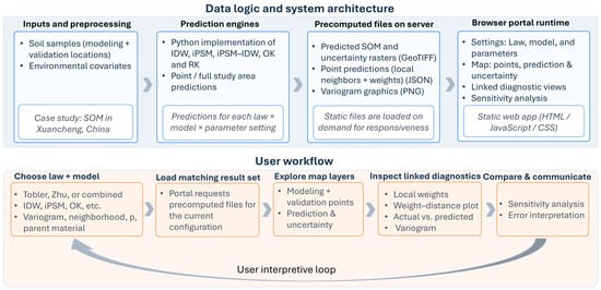
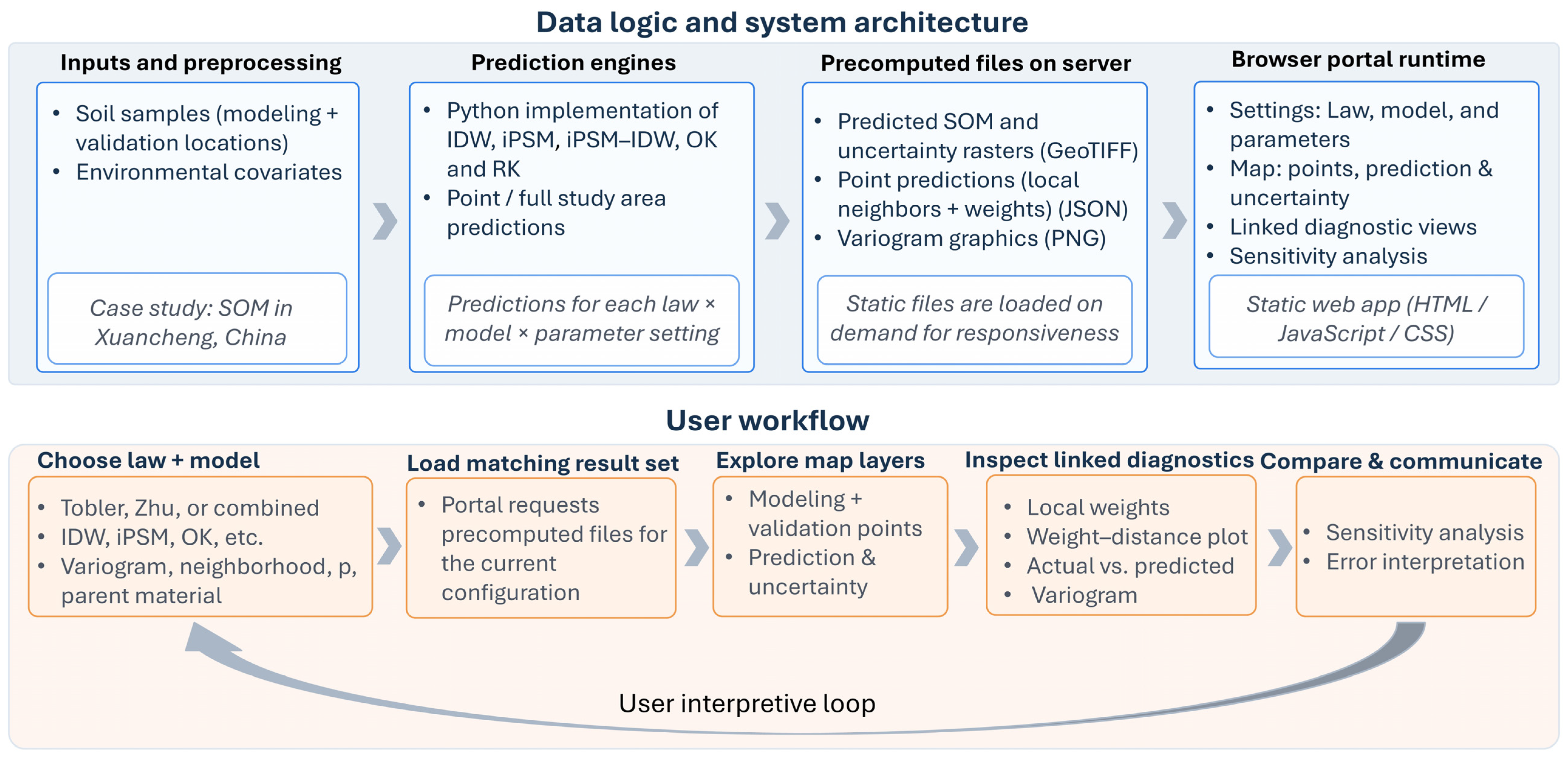
To ensure low latency in user’s interactive exploration experience, the portal does not recompute SOM predictions on-the-fly (e.g., when user switches between modeling frameworks). Instead, all modeling results, such as SOM prediction and uncertainty surfaces and predicted SOM values at the validation locations, were precomputed and stored on the web server. Upon user request (e.g., configuring/changing modeling parameters), the portal simply loads relevant data files (e.g., GeoTIFF, JSON, and PNG files) for visualization. SOM predictions were precomputed using customized Python implementations of the iPSM [44], IDW, and iPSM-IDW methods. The OK and RK methods (including automatic variogram fitting) were implemented using the scikit-gstat Python package (version 1.0.0) [42]. Figure 1 provides a conceptual level illustration of the data logic, system architecture and user workflow of the portal.

Figure 1. Data logic, system architecture and user workflow of the portal.

The web-based portal itself was developed in HTML, JavaScript, and CSS using Google’s recently released Antigravity, an IDE (integrated development environment) that supports AI agent-assisted coding. The author used a free-tier individual plan for Antigravity that offers low rate limits on backend large language models that power the AI agent (Gemini 3 Flash, Gemini 3 Pro, Claude Sonnet 4.5, Claude Opus 4.6, and GPT-OSS 120B). A high-level overview of the development process is as follows. The author (human developer) initially coded up a simplistic web page layout containing the basic elements of the portal (e.g., base map, layer control, and modeling parameter settings panel). The prototype was then exposed to the agent with descriptions of the data files and specifications of the desired user interface, functionality, and interactivity features. The agent generated a Task (and sub-Tasks) list and an Implementation Plan for review. Upon Plan approval, the agent wrote code and generated a Walkthrough document explaining the code. It then asked for code review and approval before updating the source code. The human developer was responsible for manually testing the correctness and proper functioning of the AI-generated code. When refinements, revisions, or new features are needed, the developer incrementally modified the source code directly or engaged with the agent via follow-up conversations to implement the desired changes. The portal was developed in a piecemeal and iterative fashion.

3. Results

3.1. The Geovisualization Portal

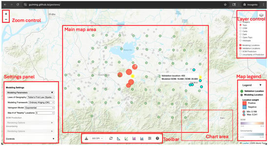
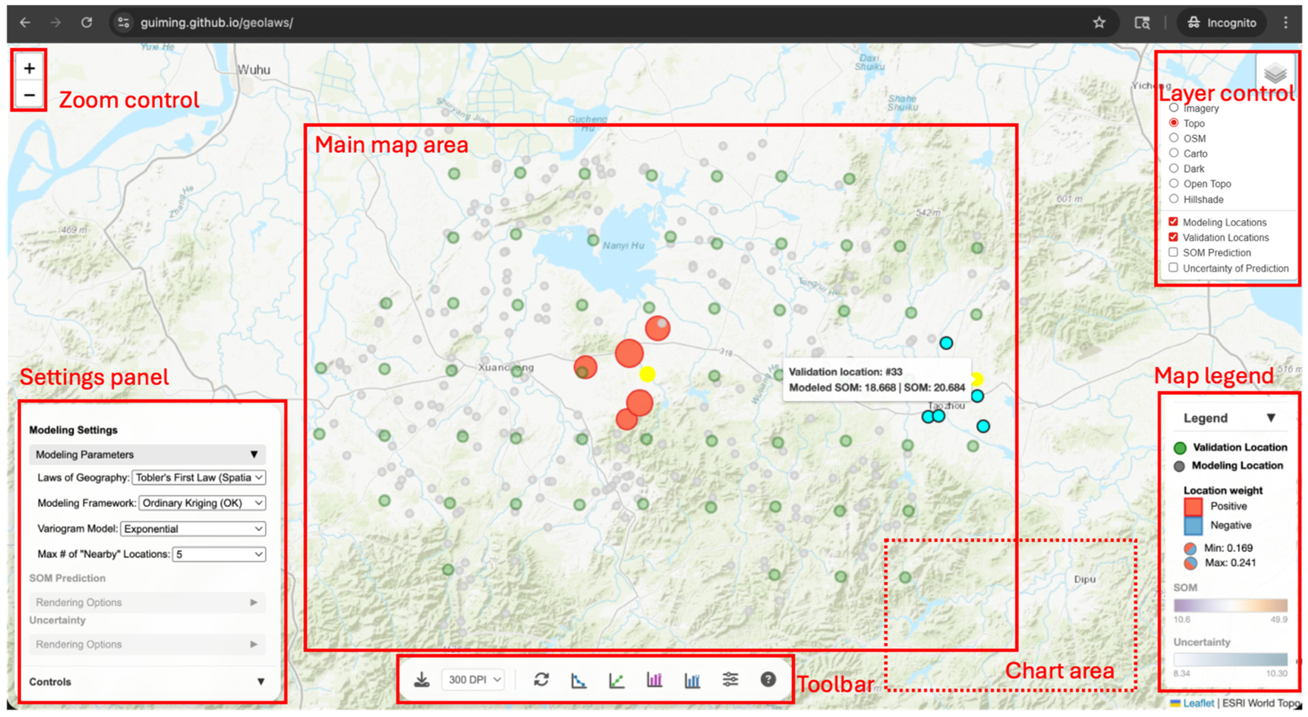
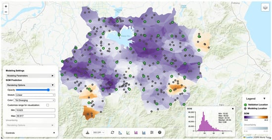
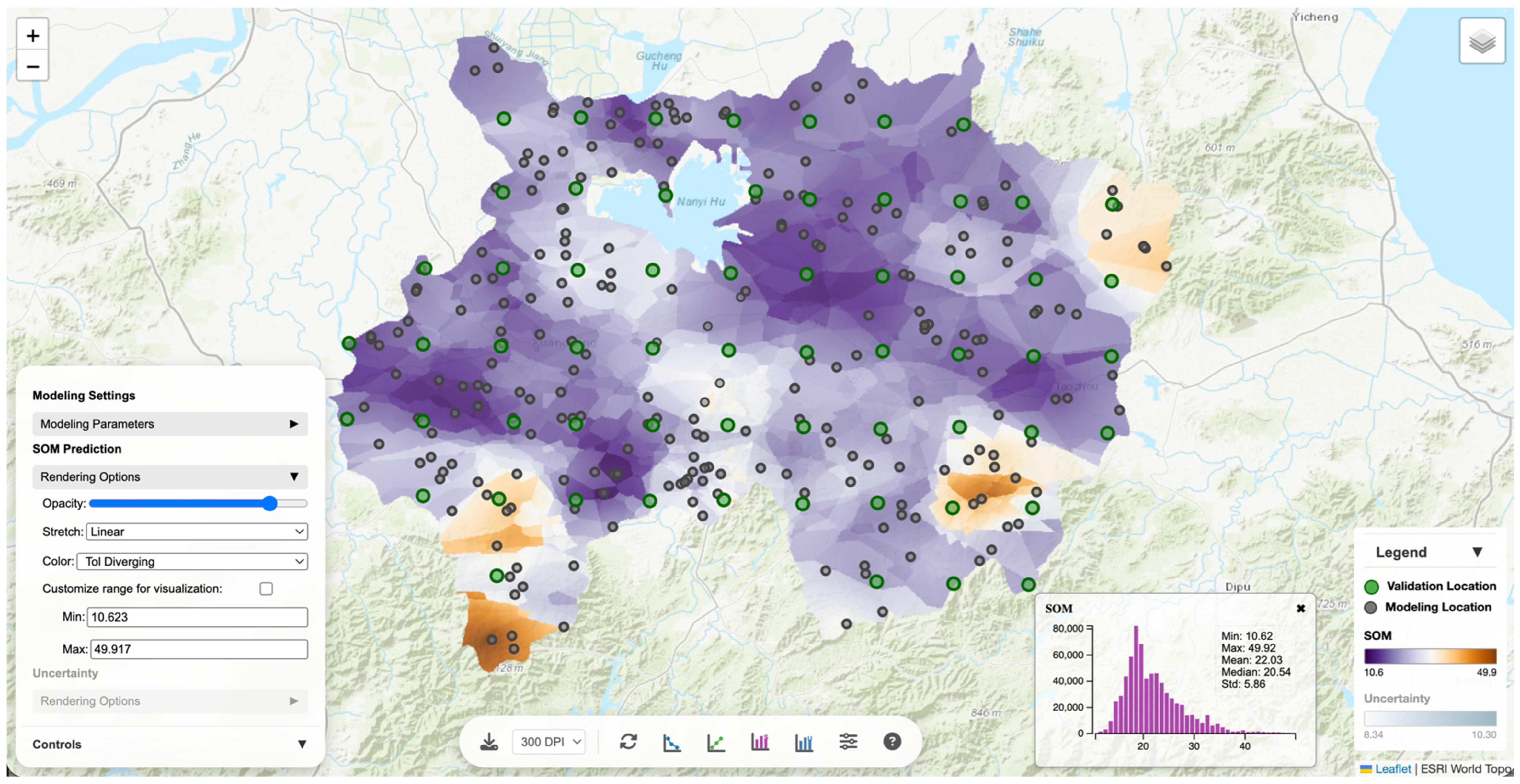
The developed geovisualization portal is deployed on GitHub and is available at https://guiming.github.io/geolaws/ (accessed on 7 May 2026). Upon loading the web portal, it displays modeling locations and validation locations over a topographic basemap with a default modeling configuration in the settings panel (i.e., Tobler’s Law, ordinary kriging, Exponential variogram, and five neighbors) (Figure 2). The portal integrates the following three major coordinated components to facilitate geovisualization-assisted exploration of the geographic laws and modeling frameworks for SOM prediction: map canvas, settings panel, and diagnostic statistical charts, as described below.

Figure 2. Basic layout of the geovisualization portal.

3.1.1. Map Canvas

The central main map area supports standard web map navigation (e.g., pan and zoom) and multiple base map options (e.g., imagery and topography). On top of the base map, modeling locations and validation locations are rendered in different styles. Regarding interactivity, hovering over a validation location allows viewing the observed and predicted SOM values at that location, while temporarily highlighting its associated modeling locations. Clicking on a validation location will persistently highlight and symbolize the associated modeling locations based on their weights. Users may check the SOM prediction and uncertainty layers in the layer control to overlay them on the map (beneath the modeling and validation locations). The map legend will dynamically update itself to show legends for the currently displayed map layers.

3.1.2. Settings Panel

The collapsible settings panel on the left-hand exposes modeling controls, including laws of geography (Tobler’s Law, Zhu’s Law, and Tobler’s and Zhu’s Laws combined), modeling framework (IDW, iPSM, iPSM-IDW, OK, and RK), variogram model (only for OK and RK; options are Spherical, Exponential, Cubic, Gaussian, and Stable), and max number of “nearby” locations (neighborhood size; options are 5, 10, 20, 30, 40, 50, and “All”). For modeling frameworks involving IDW (IDW and iPSM-IDW), a distance-decay exponent p is available. For modeling frameworks under Zhu’s Law or the combined laws that use environmental covariates (i.e., iPSM, iPSM-IDW, OK, and RK), a toggle appears for selecting whether to include parent material as a covariate. Adjusting any of these modeling parameters triggers the portal to reload data files corresponding to the current setting for visualization. The portal only allows specifying the number of “nearby” locations, a parameter comparable across the modeling frameworks. It can be an issue for kriging methods because the selection of only a few nearest sample locations may produce artifacts on the predicted map (ideally, all locations within the variogram range should all be selected).

The settings panel also provides configurable rendering options for the SOM prediction and uncertainty layers (Figure 3). It exposes opacity control and several stretch functions (linear, square-root, log, histogram equalization, percent clip, and standard deviation), along with multiple color palettes including perceptually uniform and colorblind-safe options. Users can optionally customize visualization min/max ranges to standardize rendering scales, which is useful for visual comparison across prediction/uncertainty layers resulting from different modeling settings. These options are activated only when the SOM prediction and/or uncertainty layers are visible on the map. Changing the rendering options updates rendering styles of the layers.

Figure 3. Rendering options for SOM prediction layer.

3.1.3. Diagnostic Statistical Charts

The bottom toolbar provides buttons for accessing interactive diagnostic statistical charts. These charts can be toggled on/off to display/hide in the chart area. The charts include a weight–distance scatter plot, an actual vs. predicted SOM plot, histograms of the predicted SOM and uncertainty values in the study area, and a modeling parameter sensitivity analysis panel.

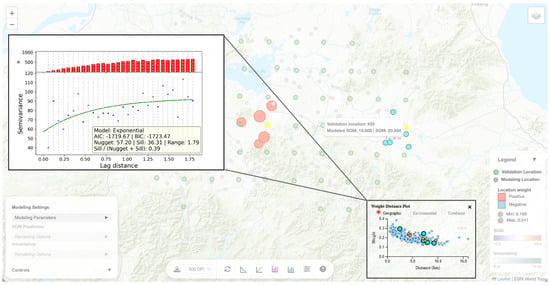
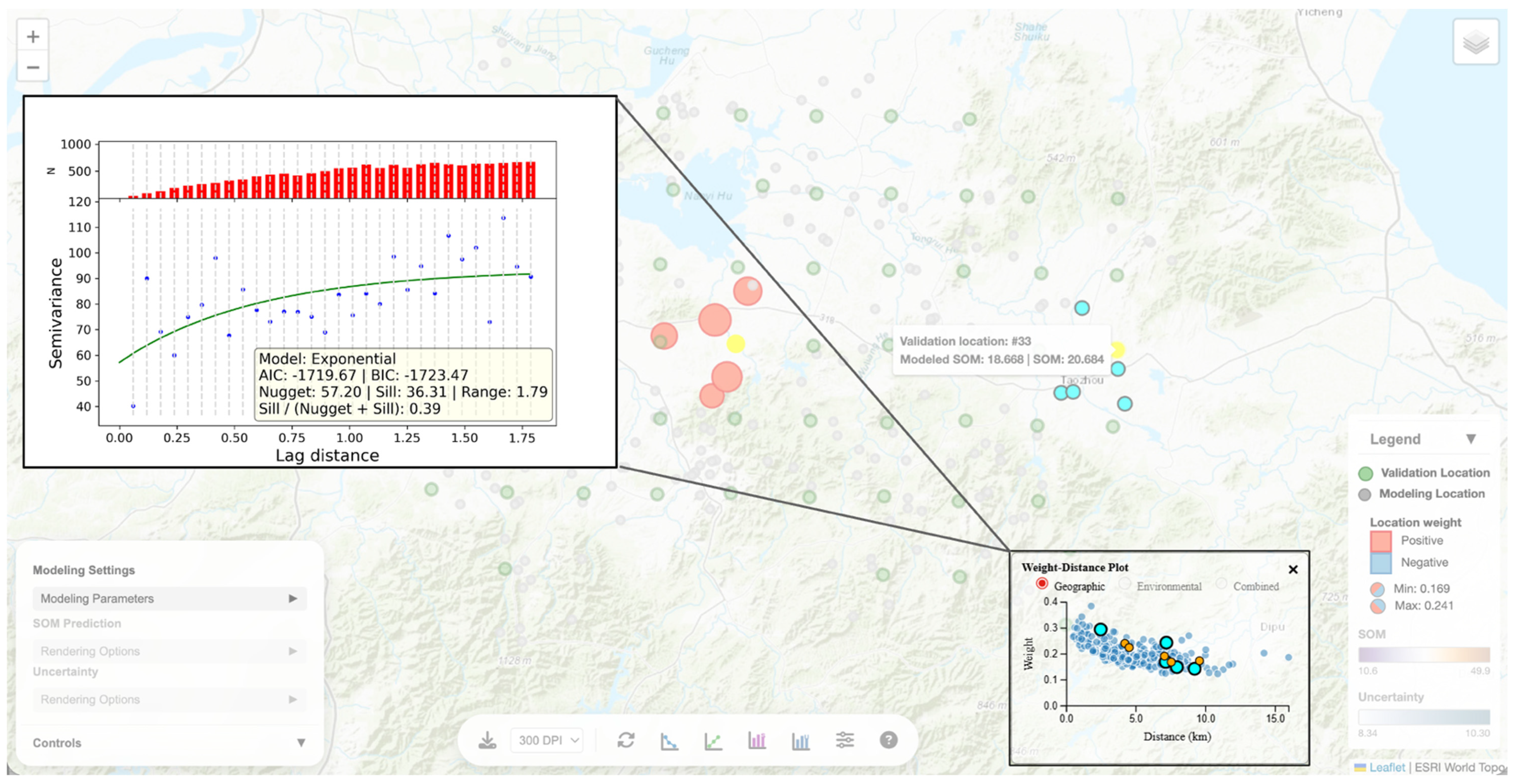
The weight–distance scatter plot visualizes how modeling location weights generally vary over geographic, environmental, or combined distance (Figure 4). Each data point on the scatter plot corresponds to a validation-modeling location pair where the point’s x and y coordinates are the distance between the pair and the weight assigned to the modeling location in predicting SOM at the validation location, respectively. Hovering over a point on the scatter plot will (temporarily) highlight the corresponding location pair on the map. Hovering/clicking on a validation location on the map (which highlights the location and its associated modeling locations) will highlight the corresponding data points on the scatter plot. Clicking on the weight-distance plot also displays the underlying fitted variogram for kriging methods. Through such linked, bi-directional map-plot interactivities, users can pursue “location explanation” of model prediction mechanics by focusing on individual validation locations to investigate how weights are distributed to its nearby modeling locations and how weight distribution is shaped by separation in geographic, environmental, or the combined space.

Figure 4. The weight-distance scatter plot and the fitted variogram model.

The actual vs. predicted scatter plot (Figure 5) visualizes prediction errors at individual validation locations and reports summary metrics for prediction accuracy, including concordance correlation coefficient (CCC), root mean squared error (RMSE), and mean absolute error (MAE). Each data point on the scatter plot represents a validation location on the map. Similar to the weight-distance plot, the actual vs. predicted plot is also linked to the map view through synchronized data point and validation location selection and highlighting. Through this plot, users can see exactly where validation locations with large prediction errors are situated in the study area and can zoom in to examine how such errors might arise.

Figure 5. The actual vs. predicted SOM scatter plot.

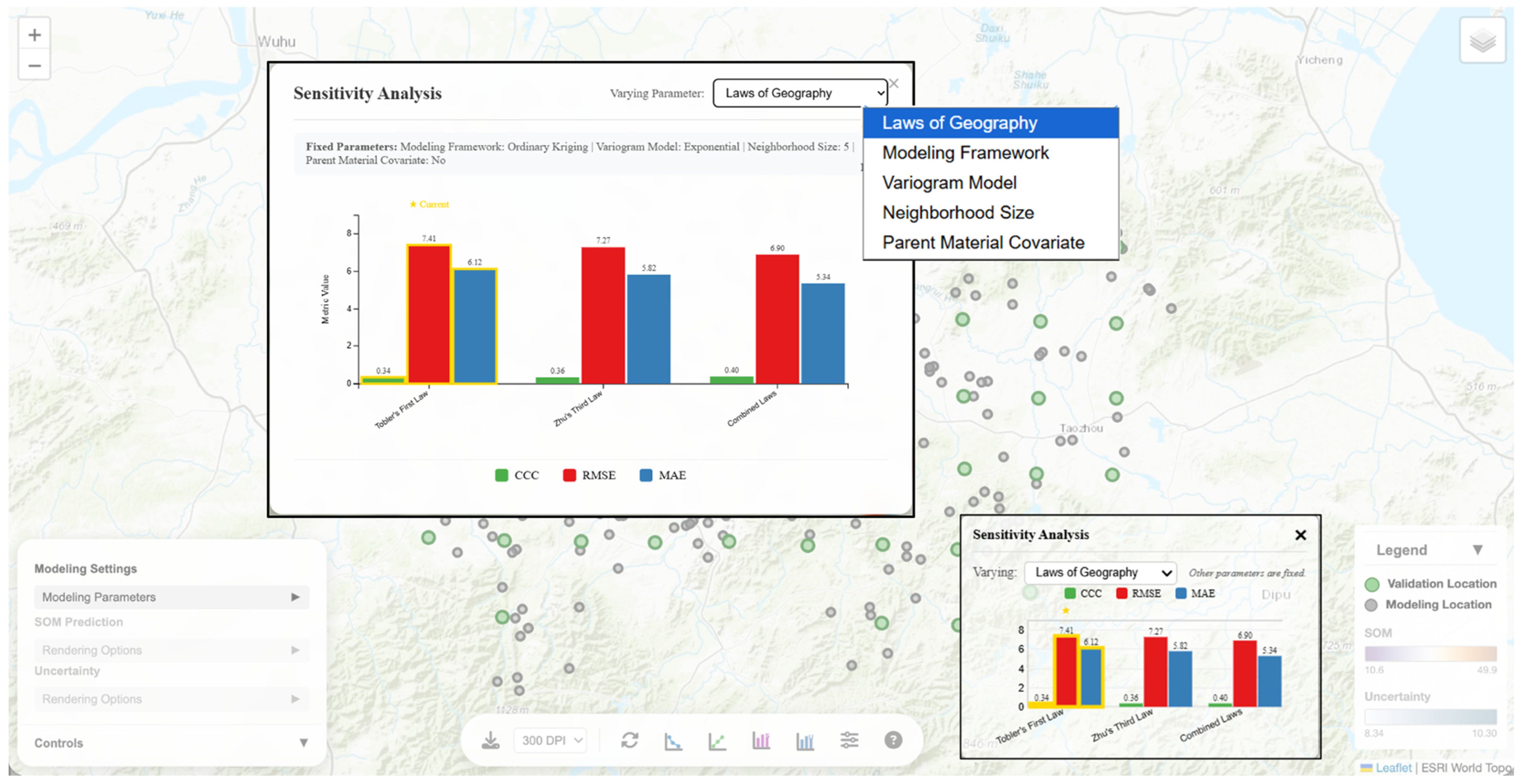
The modeling parameter sensitivity analysis panel allows users to vary one of the modeling parameters at a time (i.e., geographic law, modeling framework, neighborhood size, or when applicable, variogram, distance-decay factor or parent material covariate inclusion) while keeping other parameters fixed and visualizes how prediction accuracy metrics change over the focal parameter (Figure 6). A bar graph visualizing the metrics can be toggled on to display in the chart area. Users can also click on the bar graph to show an enlarged version to interact with. As an example, Figure 6 shows prediction metric values under the three options of geographic laws, while fixing other parameters as what are currently configured in the modeling settings (ordinary kriging, Exponential variogram, neighborhood size of five, and no parent material inclusion). Users can immediately compare and observe that, under the current parameter configuration, Tobler’s and Zhu’s Laws combined produces most accurate predictions (highest CCC and lowest RMSE and MAE).

Figure 6. The modeling parameter sensitivity analysis panel.

The toolbar also includes a reset location selection button to clear the current validation location selection and an export view function with selectable DPI (300 or 600) to export the current view as a PNG image. In a research workflow, this export function enables reproducible figure generation for side-by-side law/framework comparisons and local explanation examples that show a selected validation location and its associated modeling locations.

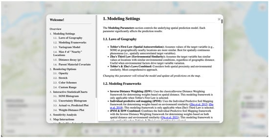
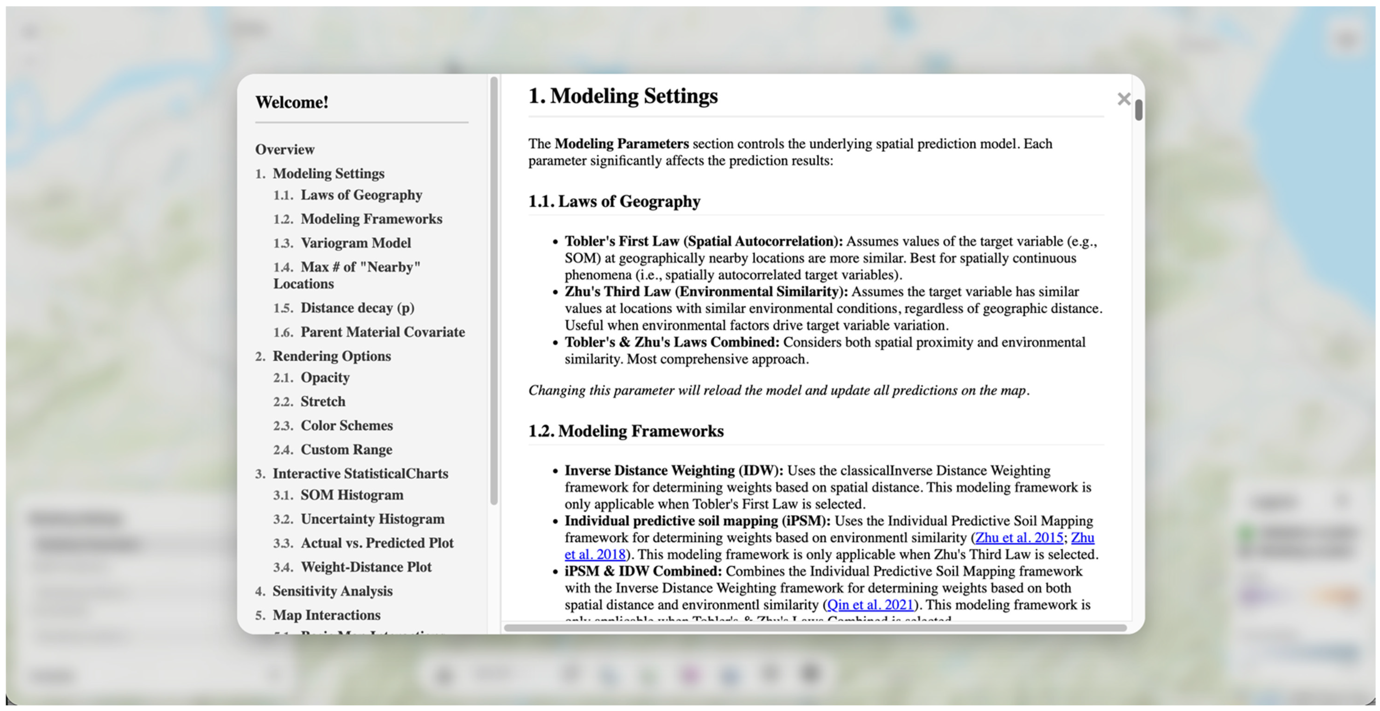
The portal also includes a modal dialog containing a user instruction manual (Figure 7) that documents each control and interaction (law/framework switching, legend behavior under selection, chart linking, and export) to help users get familiar with using this interactive geovisualization portal. The manual is accessible through an information button on the toolbar.

Figure 7. An embedded user instruction manual for the geovisualization portal.

3.2. Geovisualization-Assisted Analytical Explorations

The geovisualization portal assisted a series of analytical explorations to understand how geographic laws are embodied in a variety of modeling frameworks for DSM. Specifically, it supports workflows examining: (1) how individual predictions are made under specific geographic laws, modeling frameworks, and parameter configurations; (2) how different geographic laws manifest during the prediction process; (3) how various modeling frameworks operate; and (4) how modeling parameter settings influence prediction accuracy.

3.2.1. Analysis of Local Predictions

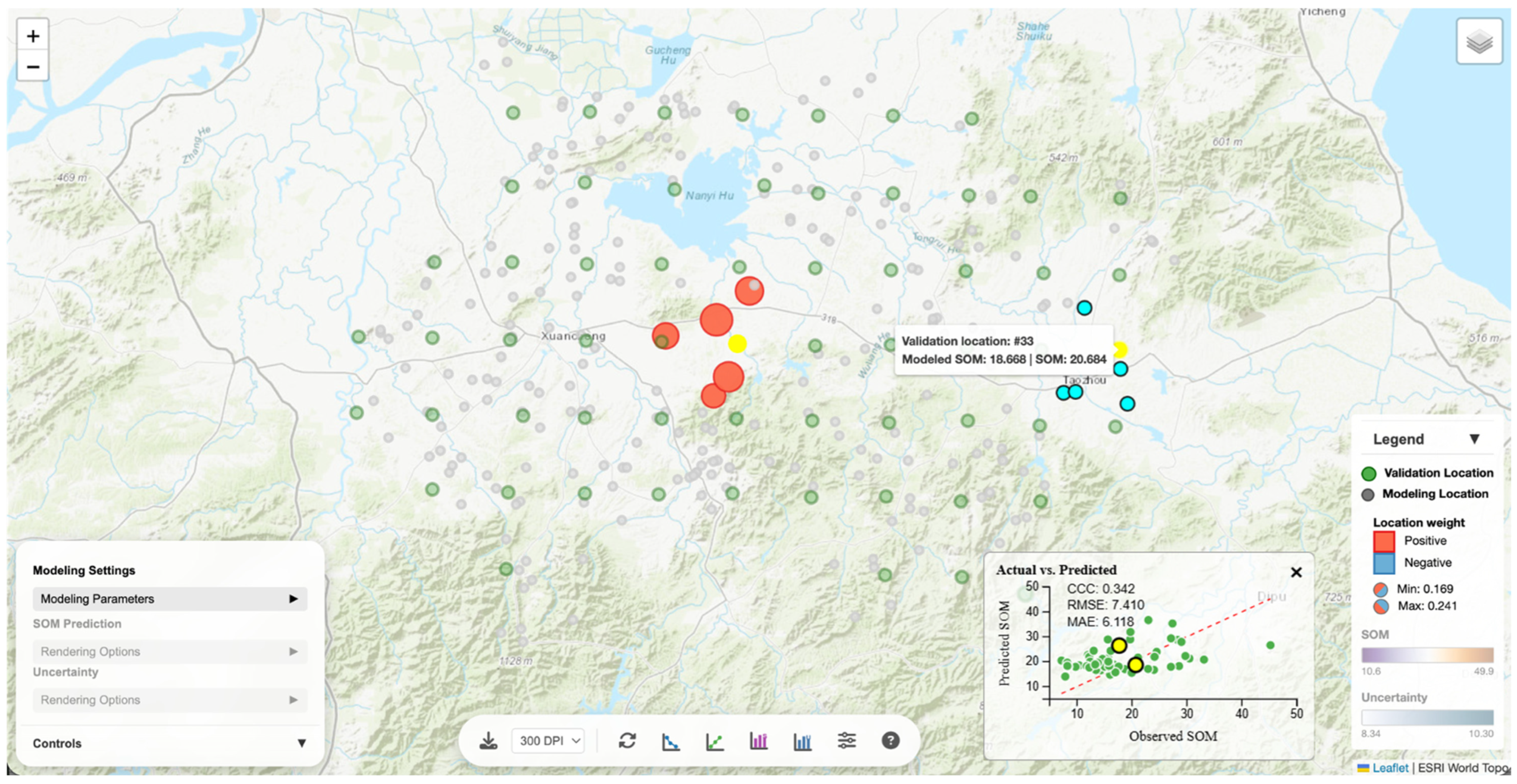
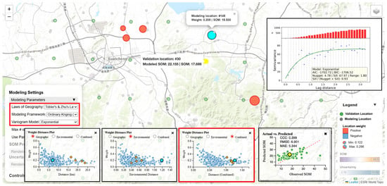
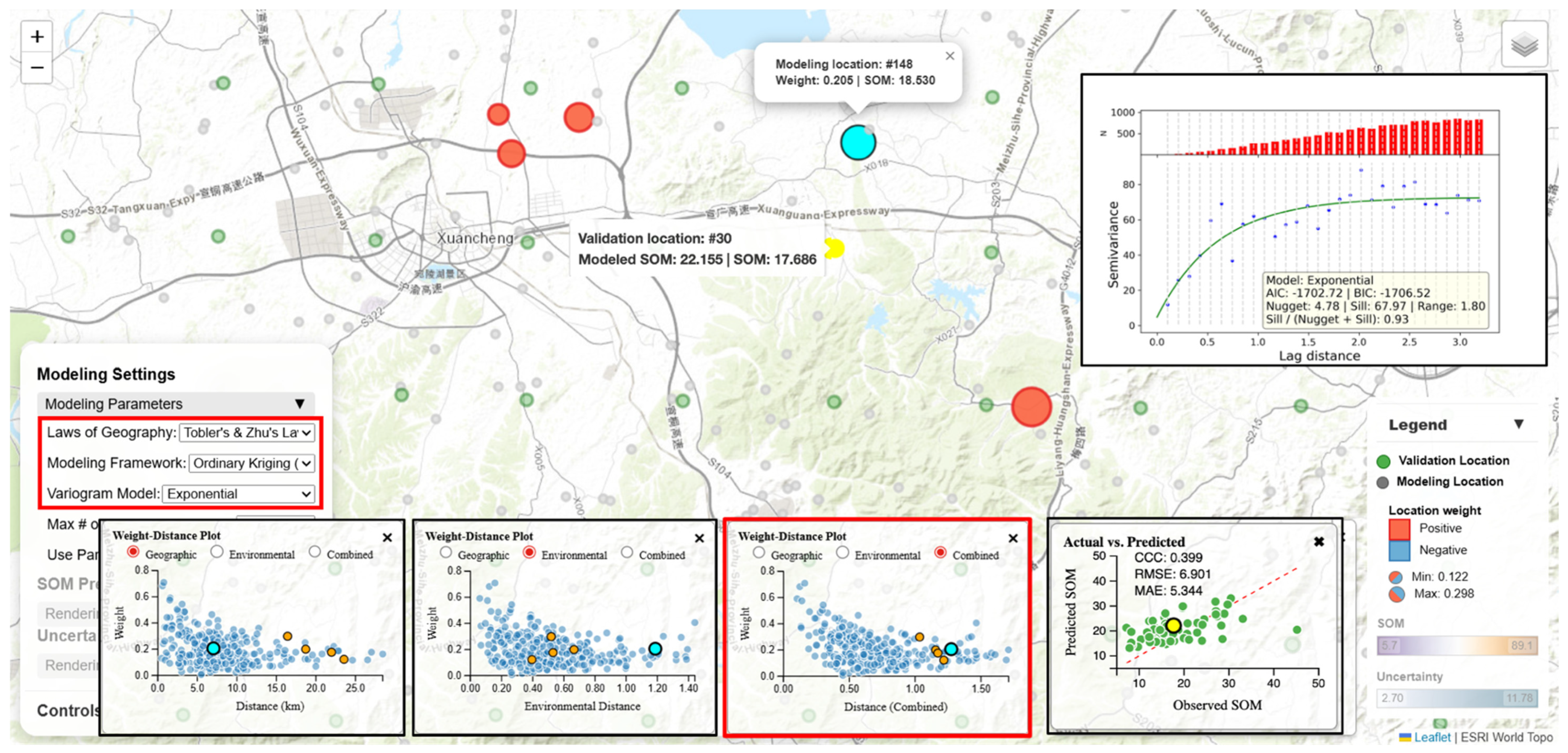
The interactive geovisualization portal facilitates local explainability of predictions. Hovering over a validation location opens a popup reporting the observed SOM value and the SOM value predicted under the current modeling settings (geographic law, modeling framework, and modeling parameter configuration). Clicking the validation location triggers highlighting of its contributing modeling locations symbolized with sizes proportional to their respective contributing weights. The dynamic legend is also updated to display weight keys (positive vs. negative influence; weight range) (Figure 8). The highlighted modeling locations are clickable and, upon clicking, a popup shows the observed SOM value at the modeling location and its contributing weight. These interactive visual displays offer a clear picture of how weights are distributed among the contributing modeling locations to produce a SOM prediction (i.e., a weighted average) at the focal validation location.

Figure 8. Local explainability of the prediction made at a validation location (highlighted in yellow) under the combined Tobler’s and Zhu’s Laws and the OK modeling framework.

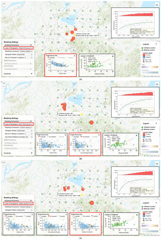
Users can further examine how modeling location weights are determined under the current modeling settings. Taking the highlighted validation location in Figure 8 as an example, the geographically closest modeling location (to the northwest) was not even contributing to the prediction under the combined Tobler’s and Zhu’s Laws and the OK modeling framework. This must be that the modeling location is so environmentally dissimilar to the validation location that it is not among the top five “nearest” neighbors of the validation location in the combined geographic-environmental space. Among the five contributing modeling locations, the geographically closest location (highlighted in bright blue) received only the second largest weight (0.205). The weight-distance scatter plots in “geographic”, “environmental”, and “combined” views shed light on why this is the case. While this modeling location is the prediction location’s nearest geographic neighbor, it is also the farthest to prediction location in the environmental space, making it overall the farthest in the combined space. The OK modeling framework assigned it the second highest weight among the five contributing neighbors based on the fitted variogram model and the underlying weight determination mechanism (Section 2.2.4).

Such analyses of local predictions make the “geographic law → modeling framework → weights → prediction” chain inspectable at specific locations, enabling users to better understand how SOM predictions are produced under a particular geographic law and modeling framework setting.

3.2.2. Manifestation of Different Geographic Laws

The portal enables visually investigating the manifestation of different geographic laws in producing predictions by holding the modeling framework constant while switching the law. The meaning of “nearby” (geographic proximity vs. environmental distance/similarity) changes under different geographic laws and therefore it affects which samples (modeling location set) influence a prediction and how strongly (weight distribution/allocation).

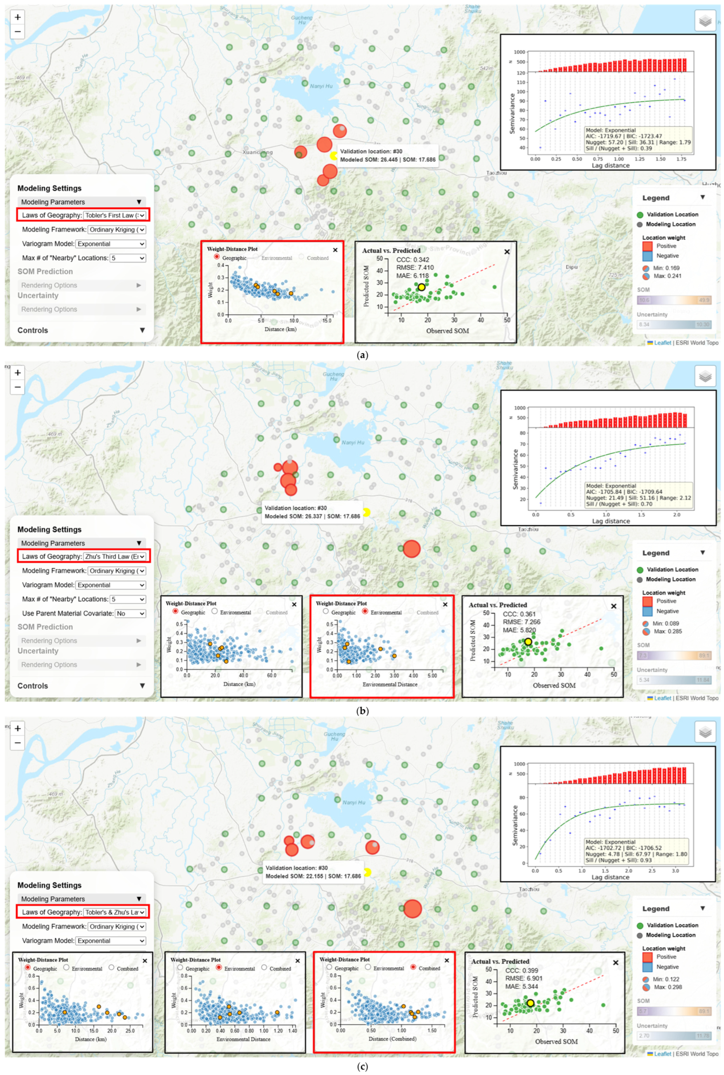
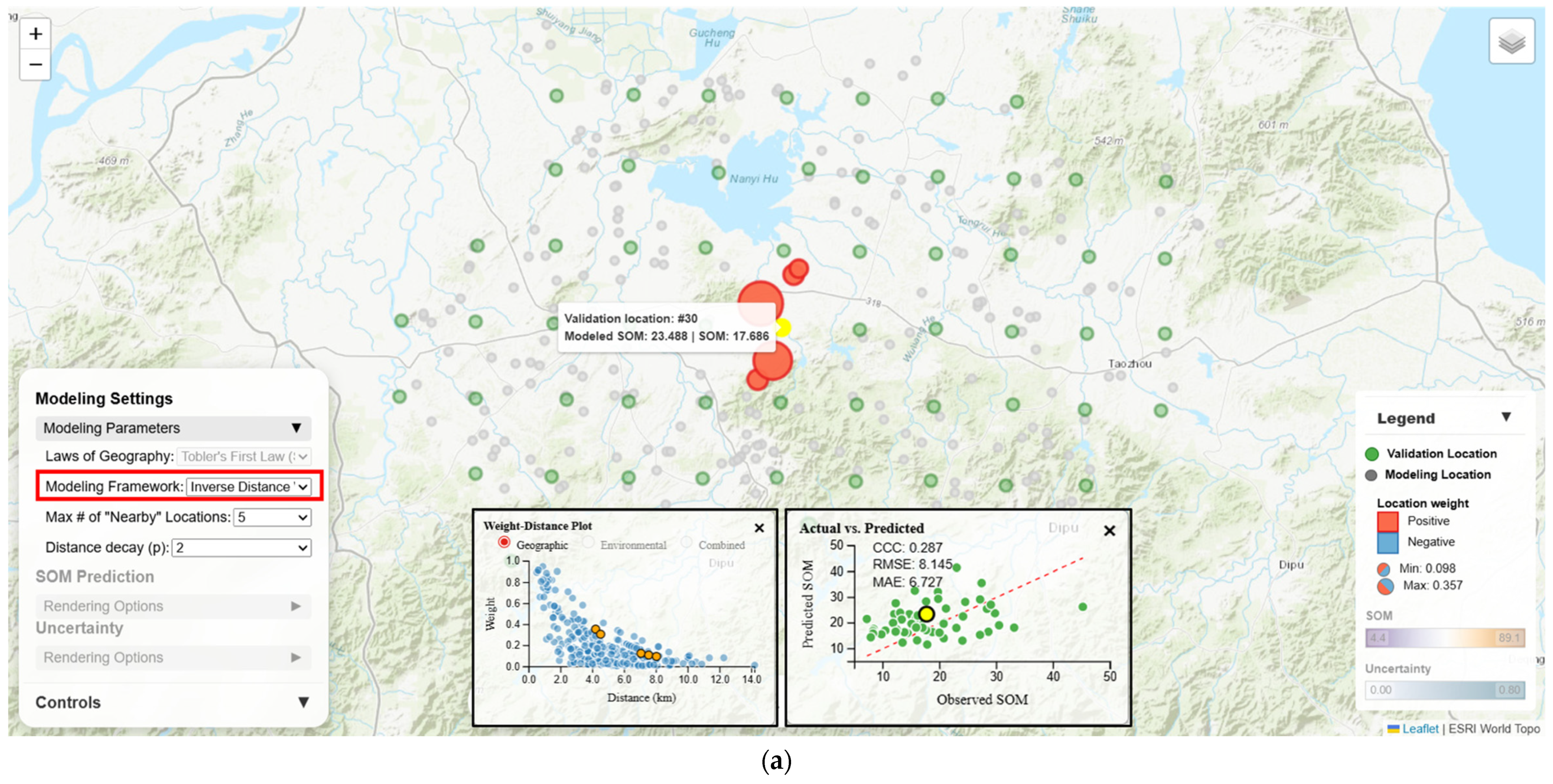
Figure 9 showcases how SOM prediction at a validation location is produced using the OK modeling framework but under three different geographic law options (Tobler’s Law, Zhu’s Law, or the two laws combined). Under Tobler’s Law, weights are distributed across five geographically nearby modeling locations following a distance-decay trend (ranging from 0.241 to 0.169) (Table 1). Under Zhu’s Law, contributing modeling locations are confined by environmental proximity instead of geographic proximity. Their weights range from 0.285 to 0.089 but weight allocation does not strictly follow environmental distance-decay (because weight allocation under OK, in principle, does not strictly follow distance-decay), with the environmentally “closest” modeling location receiving the second highest weight (0.243) and the “farthest” receiving the second lowest weight (0.153). Under the combined laws, the set of contributing modeling locations is constrained by both geographic and environmental proximity. This set shares one overlapping location with the Tobler’s Law set and three locations with the Zhu’s Law set. Weights range from 0.298 to 0.122 and the allocation follows a general distance-decay trend in the combined geographic-environmental space. For this validation location, all three geographic law options over-predict SOM, but the combined laws option resulted in the least overestimation (Table 1). Across the validation locations, this option also achieved the highest overall prediction accuracy with the highest CCC (0.399), lowest RMSE (6.901 g/kg) and lowest MAE (5.344 g/kg) (Table 1).

Figure 9. Contributing modeling locations and their weights in producing SOM prediction at a validation location using the OK modeling framework under different geographic laws: (a) Tobler’s Law (spatial autocorrelation); (b) Zhu’s Law (environmental similarity); and (c) Tobler’s and Zhu’s Laws combined.

Table 1. SOM predictions at a validation location (observed SOM is 17.686 g/kg) from the OK modeling framework under different geographic laws, and the overall prediction accuracy across all validation locations. Predicted SOM, prediction error, RMSE and MAE are in g/kg.

Geographic Law	Prediction at Validation Location #30			Overall Accuracy
	Weight Range	Predicted SOM	Prediction Error	CCC	RMSE	MAE
Tobler’s	0.241–0.169	26.445	8.759	0.342	7.410	6.118
Zhu’s	0.285–0.089	26.337	8.651	0.361	7.266	5.820
Combined	0.298–0.122	22.155	7.469	0.399	6.901	5.344

As shown in the above example, the effort to examine manifestation of the geographic laws is most informative when paired with local location selection and linked diagnostic statistical charts. Through such interactive explorations, users can observe and understand, as the geographic law in use changes, how the set of contributing modeling locations for a prediction shifts, how weight allocation pattern varies relating to geographic and/or environmental distance, and how overall prediction accuracy is impacted.

3.2.3. Comparison of Modeling Frameworks

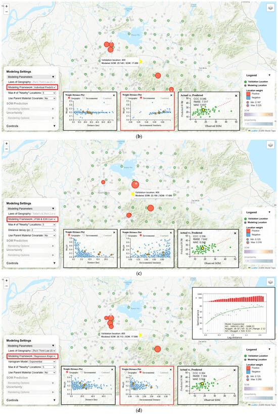
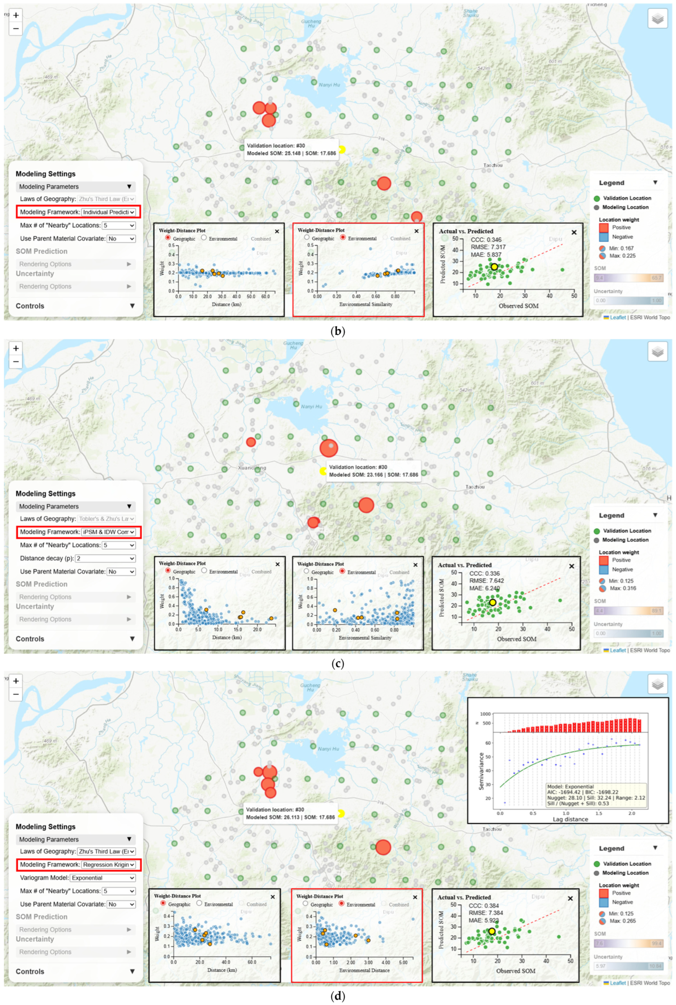
The geovisualization portal also supports users in visualizing and understanding how predictions are made by various model frameworks (IDW, iPSM, iPSM-IDW, OK, and RK) and thus enables comparing them. As an example, Figure 10 shows contributing modeling locations and their weights in producing SOM prediction at the validation location using IDW, iPSM, iPSM-IDW, and RK (OK is not included here as it was already presented in Section 3.2.2).

Figure 10. Contributing modeling locations and their weights in producing SOM prediction at a validation location under different modeling framework and geographic law choices: (a) IDW (Tobler’s Law); (b) iPSM (Zhu’s Law); (c) iPSM-IDW (combined laws); and (d) RK (Zhu’s Law).

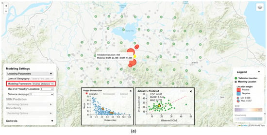
IDW (Tobler’s Law) distributes weights across the five spatial nearest neighboring modeling locations, strictly following geographic distance-decay (ranging from 0.357 to 0.098) (Table 2). iPSM (Zhu’s Law) allocates weights across the five environmentally most similar (regardless of geographic proximity) modeling locations following “dissimilarity-decay” but the weights are generally close (ranging from 0.225 to 0.167). In fact, across all validation locations, weights assigned to their respective contributing modeling locations vary only slightly in the 0.1–0.3 range over environmental similarity or geographic distance, as can be seen on the weight-distance plots (Figure 10). iPSM-IDW (combined laws) selects the top five contributing modeling locations based on the multiplication of environmental similarity and an IDW-style geographic distance weight (weights ranging from 0.316 to 0.125). These contributing modeling locations are both geographically close and environmentally similar to the prediction location. RK under Zhu’s Law distributes weights (ranging from 0.265 to 0.125) to the top five environmentally close modeling locations identical to the set of contributing modeling locations for OK under Zhu’s Law (Figure 9b). While all these frameworks overestimated the SOM concentration at the validation locations, iPSM achieved the best overall prediction accuracy (lowest RMSE of 7.317 g/kg, lowest MAE of 5.837 g/kg, and the second highest CCC of 0.346) (Table 2). Nonetheless, iPSM was still outperformed by OK under Zhu’s Law or under the combined laws (Table 1).

Table 2. SOM predictions at a validation location (observed SOM is 17.686 g/kg) from different modeling frameworks, and the overall prediction accuracy across all validation locations. Predicted SOM, prediction error, RMSE and MAE are in g/kg.

Modeling Framework (Geographic Law)	Prediction at Validation Location #30			Overall Accuracy
	Weight Range	Predicted SOM	Prediction Error	CCC	RMSE	MAE
IDW (Tobler)	0.357–0.098	23.488	5.802	0.287	8.145	6.727
iPSM (Zhu)	0.225–0.167	25.148	7.462	0.346	7.317	5.837
iPSM-IDW (Combined)	0.316–0.125	23.166	5.480	0.336	7.642	6.240
RK (Zhu)	0.265–0.125	26.113	8.427	0.384	7.384	5.923

The above example illustrates that users can observe (and make sense of) how the switching among modeling frameworks can shift the contributing modeling location set for a prediction location, alter weight allocation pattern, and impact overall prediction accuracy.

3.2.4. Evaluation of Parameter Sensitivity

Previous sections (Section 3.2.1, Section 3.2.2 and Section 3.2.3) demonstrate how the interactive map and linked charts can assist with visual explanation of local SOM predictions, investigation of geographic law manifestation in the prediction process, and comparison across modeling frameworks with respect to patterns of modeling location set selection and weight allocation and how the choice of geographic law/modeling framework affects overall prediction accuracy. Nonetheless, there are more modeling parameters beyond geographic law and modeling framework, such as neighborhood size, variogram model, distance-decay factor and whether to use parent material as a covariate. The modeling parameter sensitivity analysis panel allows users to vary one parameter, i.e., the focal parameter, at a time while keeping other parameters fixed and visualizes how prediction accuracy metrics change over the focal parameter.

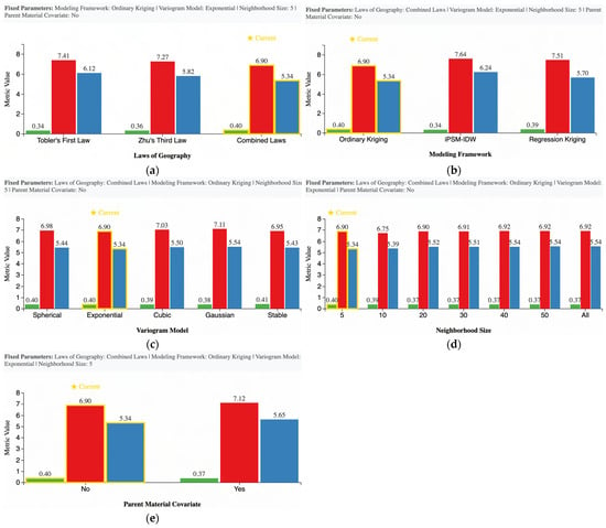
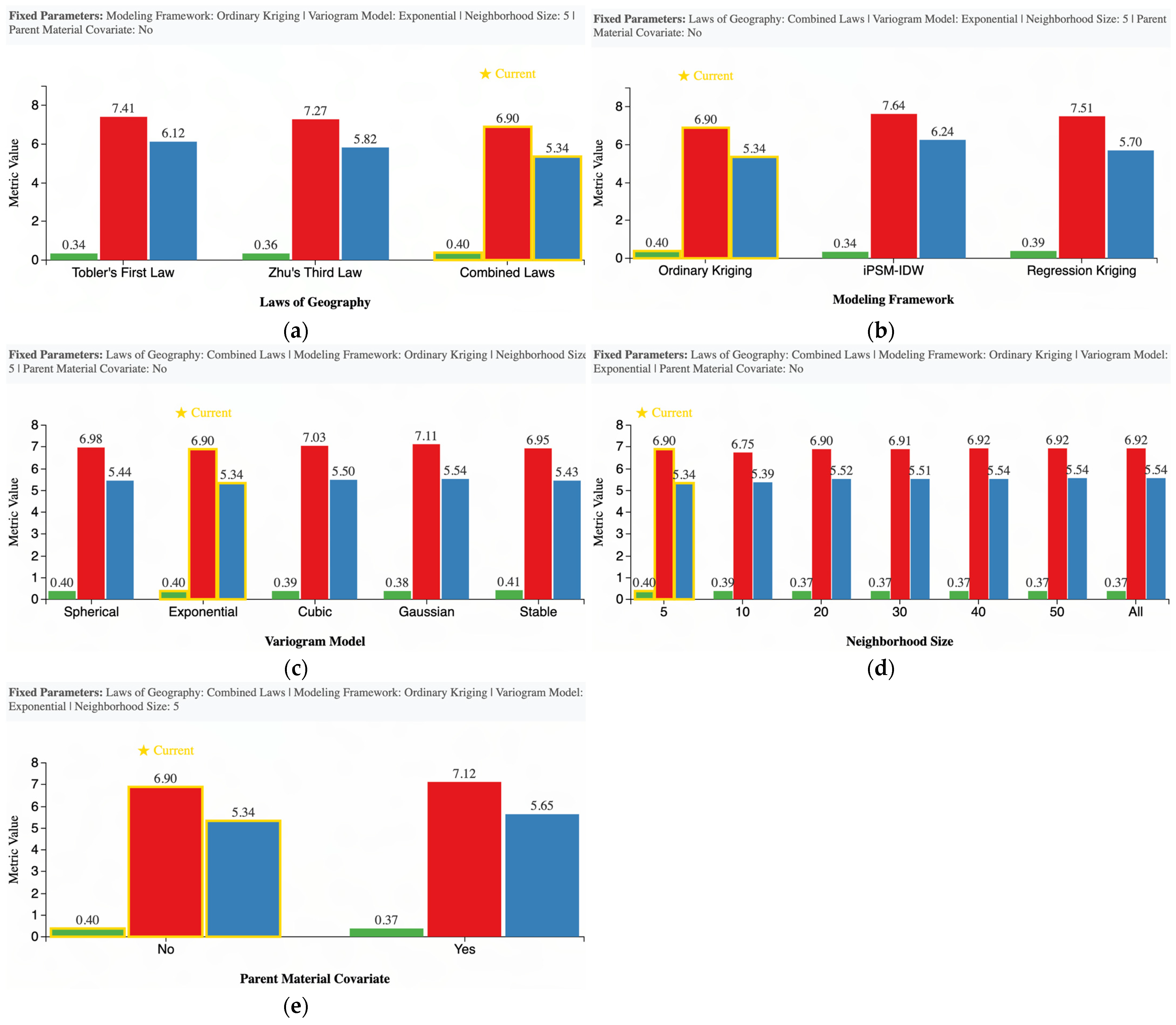
For instance, given a baseline modeling configuration (combined laws, ordinary kriging, Exponential variogram model, neighborhood size of five, and no use of parent material covariate), users can specify a focal parameter to be varied from the baseline configuration to examine how prediction accuracy metrics (i.e., CCC, RMSE, and MAE) respond to focal parameter changes. From bar graphs (Figure 11) provided through the sensitivity analysis panel, the best prediction accuracy was achieved under the combined laws (CCC = 0.40, RMSE = 6.90 g/kg, and MAE = 5.34 g/kg) followed by Zhu’s Law and Tobler’s Law, the OK modeling framework performed better than RK and iPSM-IDW, the Exponential variogram model (with the lowest RMSE and MAE and the second highest CCC) outperformed the other four model options (Spherical, Cubic, Gaussian, and Stable), the best prediction accuracy was achieved under a neighborhood size of 5 and larger neighborhood sizes seem to degrade prediction accuracy (lower CCC and higher RMSE and MAE), and finally, including parent material as a covariate for modeling slightly decreased prediction accuracy. It should be noted that the observed negative effect of parent material is specific to the particular baseline modeling configuration presented in Figure 11. Including parent material may have a positive effect under other modeling configurations (e.g., iPSM-IDW, and OK under Zhu’s Law). Also, in general, including parent material as a covariate helps differentiate bedrock types for soil formation and thus could lead to improved DSM prediction accuracy [45,46]).

Figure 11. Sensitivity of SOM prediction accuracy (as measured by CCC, RMSE, and MAE) to each modeling parameter: (a) geographic law; (b) modeling framework; (c) variogram model; (d) neighborhood size; and (e) use of parent material covariate. The baseline parameter configuration is as follows: combined laws, ordinary kriging, Exponential variogram model, neighborhood size of 5, and no use of parent material covariate. When varying the focal parameter, all other parameters were fixed to the baseline configuration.

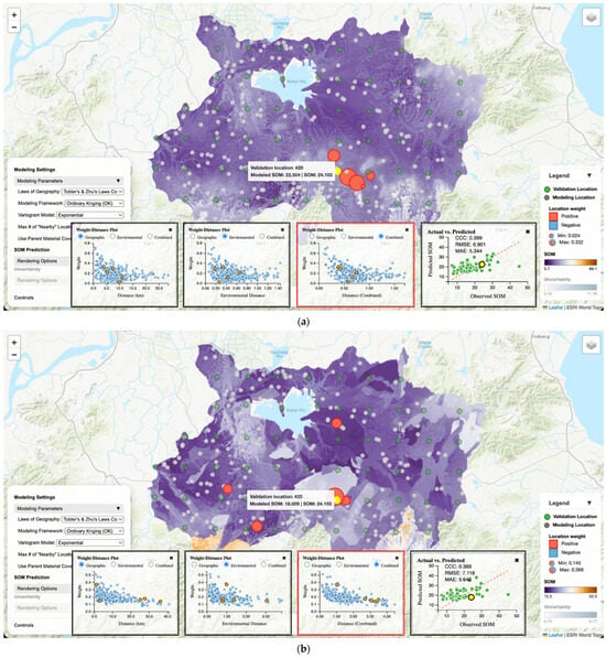
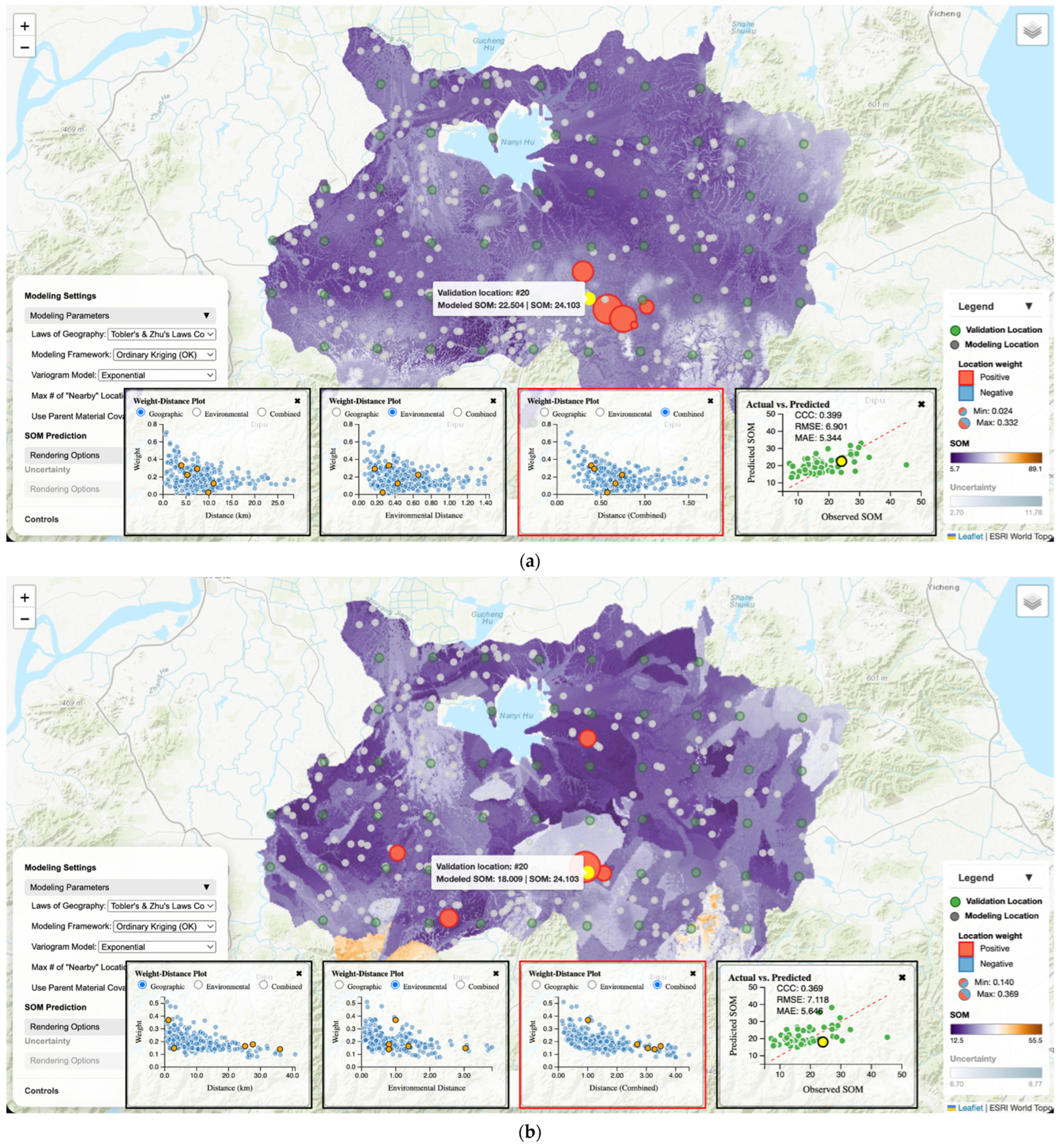
Such observations regarding sensitivity analysis could lead to follow-up explorations to understand why certain trends exist and what the finer-grain impacts of the varied parameter were. For example, to understand the impacts of parent material covariate inclusion on the prediction process, users can change the baseline configuration (in controls panel) to not include parent material for modeling and then visualize and investigate its effects on local predictions. Figure 12 shows an example of such effects in predicting SOM at a validation location. Without the parent material covariate, OK selected contributing modeling locations that are generally within the geographic vicinity of the prediction location and predicted a SOM value that is only 1.599 g/kg below the observed SOM. With parent material, the contributing modeling location set spreads widely across the study area. This occurred because locations of different parent material categories, even though they may be spatially close, would be regarded as distant in the combined geographic-environmental space (i.e., separated by a large composite distance). As a result, the (composite) distances from the prediction location to its modeling locations increased dramatically compared to not including parent material. For example, validation location in Figure 12, without parent material all five distance values are around 0.5, while without parent material four distance values are around 3.0 and one is around 1.0. This (i.e., making the prediction based on a set of much less-similar modeling locations) might partially explain the worsened underestimation of SOM (6.094 g/kg below the observed SOM).

Figure 12. SOM prediction using the OK modeling framework (with an Exponential variogram model and neighborhood size of 5) under combined Tobler’s and Zhu’s Laws: (a) parent material was not used as a covariate; (b) parent material covariate was used.

This workflow of modeling parameter sensitivity analysis and investigation makes traditionally opaque modeling decisions (e.g., covariate selection and variogram model choice) more transparent by coupling parameter changes with immediate, inspectable visualization of the effects of parameter changes.

4. Discussion

4.1. Geographic Laws as Inspectable Modeling Choices

The geovisualization portal functions as an exploratory explanation environment rather than a conventional DSM viewer that primarily disseminates final prediction layers. What differentiates the portal is that it places laws of geography alongside modeling frameworks and key parameters as interactive controls, and then immediately exposes the consequences of those choices through coordinated visual evidence. Users can switch among Tobler’s Law (spatial autocorrelation), Zhu’s Law (environmental similarity), and a combined formulation, while also changing modeling framework, neighborhood size, variogram model, and other method-specific parameters. These are not presented as abstract settings; they are tied to concrete, observable outcomes in the map canvas and the linked charts—most notably which modeling locations are selected as “nearby” contributors to the prediction, how weights are distributed across those locations, and how the predicted SOM value at a location changes.

The visually assisted analytical workflows demonstrate how this portal facilitates geographic law demystification. When a user selects a validation location, the portal reveals the contributing modeling location set under the current modeling configuration, their weights, and how those weights relate to geographic and/or environmental distance. This makes it possible to see, for a specific location, how the meaning of “nearby” shifts as the underlying geographic law changes, and how different modeling frameworks translate “nearby” into weight allocation in different ways. In this sense, the portal operationalizes geographic laws as working modeling logics that can be examined, compared, and communicated within a single geovisualization interface.

4.2. Implications for Interpretable DSM

The portal supports DSM model interpretation that is grounded in how a prediction is constructed, not only in how well it scores on global prediction accuracy metrics. DSM users often encounter a mismatch between map appearance and geographic intuition, especially in heterogeneous landscapes or under sparse and uneven sampling. By letting users move directly from an error pattern (e.g., a validation point with over- or under-estimation in the observed vs. predicted plot) to the local contributors and their weights on the map, the portal provides a concrete pathway for reasoning about why a modeling method succeeds in one area and struggles in another, enabling users to connect geographic knowledge (e.g., pedological context) to observable model behavior rather than treating the prediction layer as an opaque product.

The case study also illustrates that “better” performance can emerge from geographic law–modeling framework combinations that are not obvious from first principles. For example, Section 3.2.2 shows that, even within the same modeling framework (OK), switching the geographic law changes both the contributing location set, and the weight allocation pattern and the combined formulation produced higher overall accuracy than using Tobler’s or Zhu’s Law alone. This type of comparison is particularly valuable because many DSM discussions treat spatial autocorrelation and environmental similarity as complementary ideas but provide limited support for inspecting how those ideas manifest in local prediction processes. The portal makes that complementarity visible. Users can see when geographic proximity dominates the neighborhood, when environmental similarity dominates, and when the combined configuration yields a different compromise that can reduce prediction errors.

Finally, the sensitivity analysis panel extends interpretability from individual examples to systematic experimentation. It provides a structured way to explore trade-offs across geographic law choice, modeling framework selection, neighborhood size, variogram model, and parent material covariate inclusion, and then to follow up with location-level inspection to understand why a parameter change improved or degraded prediction accuracy. The parent material covariate example (Section 3.2.4) is illustrative. When parent material was included, contributing locations spread more widely and accuracy worsened, suggesting that how categorical factors are encoded and weighted can strongly influence what the model considers “nearby” in the combined geographic-environmental space. Such findings are difficult to diagnose from accuracy metrics alone but become interpretable when parameter sensitivity and local explanation are tightly linked. In any cases, the emphasis and contribution of the geovisualization portal lies more in increasing the explainability of DSM models rather than in improving DSM accuracy.

4.3. Limitations and Future Work

Several limitations shape how the portal should be interpreted and how it can be extended. First, the demonstration is based on a single study area and one soil property (SOM) with a specific validation design (a 10 km × 10 km grid for validation locations). While the portal’s interaction logic is general, conclusions about which geographic law or modeling framework “performs best” should not be generalized beyond this setting without additional case studies across soil properties, landscapes, and sampling regimes.

Second, the portal emphasizes responsiveness by loading precomputed outputs rather than recomputing predictions on demand (Section 2.3). This supports smooth exploration within a defined parameter grid, but it limits the ability to perform free-form experimentation (e.g., continuous tuning of neighborhood size or distance-decay parameters, adding new covariates on the fly, or interactively refitting variograms). A natural extension is to support hybrid operation modes—precomputed results for common settings paired with optional server-side computation for user-defined configurations.

Future development can also broaden the modeling scope. While this study focused on five transparent and widely used frameworks (IDW, iPSM, iPSM-IDW, OK, and RK), extending the portal to additional DSM families (e.g., geographically weighted models and selected machine-learning approaches) would allow the same geographic law-centered interpretation questions to be asked across a wider methodological spectrum. The core contribution demonstrated here—coordinated, location-centered explanation tied to explicit geographic law choices—provides a template for those extensions.

5. Conclusions

This study developed a web-based interactive geovisualization portal to support visually assisted sense-making of how laws of geography are embodied in DSM modeling frameworks. The portal enables users to toggle among Tobler’s First Law, Zhu’s Third Law, and a combined formulation, and to examine how these choices interact with five commonly used spatial prediction frameworks (IDW, iPSM, iPSM-IDW, OK, and RK). Through coordinated interactions between the map and linked diagnostic charts, the portal makes local prediction construction inspectable by revealing contributing modeling locations, their weights, and how weights relate to geographic, environmental, or combined distance. It also integrates prediction and uncertainty layers with configurable rendering, links prediction errors to map locations, and provides a sensitivity-analysis workflow that connects parameter changes to both global accuracy metrics and local prediction behavior.

Using SOM mapping in the Xuancheng study area as an example, the portal demonstrated how switching the geographic law can change which soil samples are treated as “nearby”, how weights are allocated, and how local prediction errors and global prediction accuracy respond. The sensitivity-analysis workflow further showed that key modeling decisions—such as geographic law, modeling framework, neighborhood size, variogram model choice, and categorical covariate inclusion—can materially influence prediction outcomes and can be diagnosed through follow-up local inspection. Overall, the portal’s primary contribution is an interactive environment that demystifies geographic laws for DSM by supporting explanation, comparison, and communication of DSM modeling logic in a manner consistent with geovisualization principles of coordinated views and exploratory analysis.

References

- Adhikari, K.; Owens, P.R.; Libohova, Z.; Miller, D.M.; Wills, S.A.; Nemecek, J. Assessing soil organic carbon stock of Wisconsin, USA and its fate under future land use and climate change. Sci. Total Environ. 2019, 667, 833–845. [Google Scholar] [CrossRef] [Scilit]
- Minasny, B.; McBratney, A.B.; Malone, B.P.; Wheeler, I. Digital Mapping of Soil Carbon. In Advances in Agronomy; Elsevier: Amsterdam, The Netherlands, 2013; Volume 118, pp. 1–47. ISBN 9780124059429. [Google Scholar]
- Scharlemann, J.P.W.; Tanner, E.V.J.; Hiederer, R.; Kapos, V. Global soil carbon: Understanding and managing the largest terrestrial carbon pool. Carbon Manag. 2014, 5, 81–91. [Google Scholar] [CrossRef] [Scilit]
- Batjes, N.H.; Ribeiro, E.; Van Oostrum, A.; Leenaars, J.; Hengl, T.; Mendes De Jesus, J. WoSIS: Providing standardised soil profile data for the world. Earth Syst. Sci. Data 2017, 9, 1–14. [Google Scholar] [CrossRef] [Scilit]
- Batjes, N.H.; Ribeiro, E.; Van Oostrum, A. Standardised soil profile data to support global mapping and modelling (WoSIS snapshot 2019). Earth Syst. Sci. Data 2020, 12, 299–320. [Google Scholar] [CrossRef] [Scilit]
- McBratney, A.; Mendonça Santos, M.; Minasny, B. On digital soil mapping. Geoderma 2003, 117, 3–52. [Google Scholar] [CrossRef] [Scilit]
- Minasny, B.; McBratney, A.B. Digital soil mapping: A brief history and some lessons. Geoderma 2016, 264, 301–311. [Google Scholar] [CrossRef] [Scilit]
- Wadoux, A.M.J.C.; Minasny, B.; McBratney, A.B. Machine learning for digital soil mapping: Applications, challenges and suggested solutions. Earth-Sci. Rev. 2020, 210, 103359. [Google Scholar] [CrossRef] [Scilit]
- Zhao, F.; Zhu, A.; Zhu, L.; Qin, C. iSoLIM: A similarity-based spatial prediction software for the big data era. Ann. GIS 2024, 30, 535–549. [Google Scholar] [CrossRef] [Scilit]
- Jiang, J.; Zhu, A.-X.; Qin, C.-Z.; Zhu, T.; Liu, J.; Du, F.; Liu, J.; Zhang, G.; An, Y. CyberSoLIM: A cyber platform for digital soil mapping. Geoderma 2016, 263, 234–243. [Google Scholar] [CrossRef] [Scilit]
- Goodchild, M.F. Commentary: General principles and analytical frameworks in geography and GIScience. Ann. GIS 2022, 28, 85–87. [Google Scholar] [CrossRef] [Scilit]
- Goodchild, M.F. The validity and usefulness of laws in geographic information science and geography. Ann. Assoc. Am. Geogr. 2004, 94, 300–303. [Google Scholar] [CrossRef] [Scilit]
- Tobler, W.R. A computer movie simulating urban growth in the Detroit region. Econ. Geogr. 1970, 46, 234–240. [Google Scholar] [CrossRef] [Scilit]
- Diggle, P.J.; Ribeiro, P.J. Model-Based Geostatistics; Springer: Berlin/Heidelberg, Germany, 2007. [Google Scholar]
- Hengl, T.; Heuvelink, G.B.M.; Stein, A. A generic framework for spatial prediction of soil variables based on regression-kriging. Geoderma 2004, 120, 75–93. [Google Scholar] [CrossRef] [Scilit]
- Goovaerts, P. Geostatistics for Natural Resources Evaluation; Oxford University Press: Oxford, UK, 1997; ISBN 0195115384. [Google Scholar]
- Isaaks, E.H.; Srivastava, R.M. An Introduction to Applied Geostatistics; Oxford University Press: New York, NY, USA, 1989; ISBN 0-19-505012-6. [Google Scholar]
- Zhu, A.; Lu, G.; Liu, J.; Qin, C.; Zhou, C. Spatial prediction based on Third Law of Geography. Ann. GIS 2018, 24, 225–240. [Google Scholar] [CrossRef] [Scilit]
- Zhu, A.X.; Turner, M. How is the Third Law of Geography different? Ann. GIS 2022, 28, 57–67. [Google Scholar] [CrossRef] [Scilit]
- Zhu, A.X.; Hudson, B.; Burt, J.; Lubich, K.; Simonson, D. Soil mapping using GIS, expert knowledge, and fuzzy logic. Soil Sci. Soc. Am. J. 2001, 65, 1463–1472. [Google Scholar] [CrossRef] [Scilit]
- Zhu, A.-X.; Liu, J.; Du, F.; Zhang, S.; Qin, C.-Z.; Burt, J.; Behrens, T.; Scholten, T. Predictive soil mapping with limited sample data. Eur. J. Soil Sci. 2015, 66, 535–547. [Google Scholar]
- Fan, X.; Fan, N.; Qin, C.Z.; Zhao, F.H.; Zhu, L.J.; Zhu, A.X. Large-area soil mapping based on environmental similarity with adaptive consideration of spatial distance to samples. Geoderma 2023, 439, 116683. [Google Scholar] [CrossRef] [Scilit]
- Qin, C.-Z.; An, Y.; Liang, P.; Zhu, A.-X.; Yang, L. Soil property mapping by combining spatial distance information into the Soil Land Inference Model (SoLIM). Pedosphere 2021, 31, 638–644. [Google Scholar] [CrossRef] [Scilit]
- Guo, P.-T.; Li, W.-T.; Li, M.-F.; Yan, P.-S.; Liu, Y.; Zhao, J. The iPSM-SD Framework: Enhancing Predictive Soil Mapping for Precision Agriculture Through Spatial Proximity Integration. Agronomy 2026, 16, 231. [Google Scholar] [CrossRef] [Scilit]
- Kraak, M.-J. Geovisualization illustrated. ISPRS J. Photogramm. Remote Sens. 2003, 57, 390–399. [Google Scholar] [CrossRef] [Scilit]
- MacEachren, A.M.; Kraak, M.-J. Research Challenges in Geovisualization. Cartogr. Geogr. Inf. Sci. 2001, 28, 3–12. [Google Scholar] [CrossRef] [Scilit]
- Çöltekin, A.; Bleisch, S.; Andrienko, G.; Dykes, J. Persistent challenges in geovisualization–a community perspective. Int. J. Cartogr. 2017, 3, 115–139. [Google Scholar] [CrossRef] [Scilit]
- Geostokos (Ecosse) Limited. Kriging Game Teaching Software, version 2009; Geostokos (Ecosse) Limited: Alloa, Scotland, 2019.
- Walvoort, D. E{Z}-Kriging: Exploring the World of Ordinary Kriging; Wageningen University & Research: Wageningen, The Netherlands, 2004. [Google Scholar]
- Roth, R.E. Interactive maps: What we know and what we need to know. J. Spat. Inf. Sci. 2013, 2013, 59–115. [Google Scholar] [CrossRef] [Scilit]
- Zhang, G. A web-based geovisualization framework for exploratory analysis of individual VGI contributor’s participation characteristics. Cartogr. Geogr. Inf. Sci. 2025, 52, 199–219. [Google Scholar] [CrossRef] [Scilit]
- Zhang, G.; Luo, W.; Wu, M.; Ye, L. Exploring social interaction patterns and drivers in VGI communities using a custom geovisual analytics tool. Ann. GIS 2025, 31, 413–431. [Google Scholar] [CrossRef] [Scilit]
- Hengl, T.; De Jesus, J.M.; Heuvelink, G.B.M.; Gonzalez, M.R.; Kilibarda, M.; Blagotić, A.; Shangguan, W.; Wright, M.N.; Geng, X.; Bauer-Marschallinger, B.; et al. SoilGrids250m: Global gridded soil information based on machine learning. PLoS ONE 2017, 12, e0169748. [Google Scholar] [CrossRef] [Scilit]
- Poggio, L.; De Sousa, L.M.; Batjes, N.H.; Heuvelink, G.B.M.; Kempen, B.; Ribeiro, E.; Rossiter, D. SoilGrids 2.0: Producing soil information for the globe with quantified spatial uncertainty. Soil 2021, 7, 217–240. [Google Scholar]
- Hengl, T.; Heuvelink, G.B.M.; Rossiter, D.G. About regression-kriging: From equations to case studies. Comput. Geosci. 2007, 33, 1301–1315. [Google Scholar] [CrossRef] [Scilit]
- Zeng, C.; Yang, L.; Zhu, A.-X.; Rossiter, D.G.; Liu, J.; Liu, J.; Qin, C.; Wang, D. Mapping soil organic matter concentration at different scales using a mixed geographically weighted regression method. Geoderma 2016, 281, 69–82. [Google Scholar] [CrossRef] [Scilit]
- Zhu, D.; Liu, Y.; Yao, X.; Fischer, M.M. Spatial regression graph convolutional neural networks: A deep learning paradigm for spatial multivariate distributions. Geoinformatica 2023, 27, 641–642. [Google Scholar] [CrossRef] [Scilit]
- Zhang, S.; Zhu, A.-X.; Liu, J.; Yang, L.; Qin, C.-Z.; An, Y.-M. An heuristic uncertainty directed field sampling design for digital soil mapping. Geoderma 2016, 267, 123–136. [Google Scholar] [CrossRef] [Scilit]
- Yang, L.; Qi, F.; Zhu, A.-X.; Shi, J.; An, Y. Evaluation of Integrative Hierarchical Stepwise Sampling for Digital Soil Mapping. Soil Sci. Soc. Am. J. 2016, 80, 637–651. [Google Scholar] [CrossRef] [Scilit]
- Yang, L.; Zhu, A.X.; Zhao, Y.; Li, D.; Zhang, G.; Zhang, S.; Band, L.E. Regional Soil Mapping Using Multi-Grade Representative Sampling and a Fuzzy Membership-Based Mapping Approach. Pedosphere 2017, 27, 344–357. [Google Scholar] [CrossRef] [Scilit]
- Cressie, N. Statistics for Spatial Data; John Wiley & Sons: New York, NY, USA, 1993; ISBN 1119115183. [Google Scholar]
- Mälicke, M. SciKit-GStat 1.0: A SciPy-flavored geostatistical variogram estimation toolbox written in Python. Geosci. Model Dev. 2022, 15, 2505–2532. [Google Scholar] [CrossRef] [Scilit]
- Zhao, F.H.; Zhu, A.X.; Qin, C.Z. Spatial distribution pattern analysis using variograms over geographic and feature space. Geo-Spat. Inf. Sci. 2025, 28, 1774–1788. [Google Scholar] [CrossRef] [Scilit]
- Zhang, G.; Zhu, A.-X.; Liu, J.; Guo, S.; Zhu, Y. PyCLiPSM: Harnessing heterogeneous computing resources on CPUs and GPUs for accelerated digital soil mapping. Trans. GIS 2021, 25, 1396–1418. [Google Scholar] [CrossRef] [Scilit]
- Cahyana, D.; Sulaeman, Y.; Barus, B.; Mulyanto, B. Improving digital soil mapping in Bogor, Indonesia using parent material information. Geoderma Reg. 2023, 33, e00627. [Google Scholar] [CrossRef] [Scilit]
- Ma, Y.; Minasny, B.; Malone, B.P.; Mcbratney, A.B. Pedology and digital soil mapping (DSM). Eur. J. Soil Sci. 2019, 70, 216–235. [Google Scholar] [CrossRef] [Scilit]
Disclaimer/Publisher’s Note: The statements, opinions and data contained in all publications are solely those of the individual author(s) and contributor(s) and not of MDPI and/or the editor(s). MDPI and/or the editor(s) disclaim responsibility for any injury to people or property resulting from any ideas, methods, instructions or products referred to in the content. |
© 2026 by the author. Published by MDPI on behalf of the International Society for Photogrammetry and Remote Sensing. Licensee MDPI, Basel, Switzerland. This article is an open access article distributed under the terms and conditions of the Creative Commons Attribution (CC BY) license.