


Abstract
Activity space represents the spatiotemporal interaction between individuals and their environment. While most studies measure potential activity space using short-term data, few have defined or measured its actual internal structure. This study introduces “anchor regions” as the core areas where daily activities are concentrated, and conceptualizes the structure of an individual’s activity space by incorporating the concept of regular locations, anchor regions, potential regular activity space, and potential activity space. Using three months of mobile signaling data from 10,848 residents in Shenzhen, we detected anchor regions via a weighted density-based spatial clustering for applications with noise (DBSCAN) method and categorized individuals into six typical activity space structures based on a rule-based taxonomy. We also figured out the intra- and inter-anchor region mobility pattern of each type. Our results show the following: (1) A total of 80% of activities and 87% of time are concentrated in just 26% of locations, forming anchor regions—with 95% of individuals having no more than five such regions. (2) The total area of anchor regions is merely 0.1% of the potential activity space. (3) Six typical structures of activity space are derived with different combinations of several functional anchor regions, including home, weekday anchors, and daily activity anchors. (4) The spatial patterns of the six types are different, while intra-anchor region mobilities dominate daily movement in all six types. This study provides a region-based, instead of a point-based, perspective interpretation of the anchor points theory, helping to better understand the regularities and internal structure of human activity space. Our conceptual framework and methodology have the potential to help urban and transportation planning practice and policy making.
1. Introduction
Activity space has been widely discussed as a concept representing the spatiotemporal interaction between individuals and the environment [1]. It generally refers to the spatial environment where people’s daily activities and trips take place [2]. The concept is particularly relevant to mobility, accessibility, and transportation research, helping us understand human mobility patterns [3,4,5], social exclusion [6,7,8], and environmental exposure [9,10,11]. Empirically, its measurement often employs spatial analytical techniques, such as standard deviation ellipses, minimum convex polygons, kernel density surfaces, and road network buffers [6,12,13].
Although activity space in most of the literature often refers to an ideal areal scope that people can potentially reach under certain constraints, namely, potential activity space [14,15], in reality it is full of spatial heterogeneities with an internal spatial structure [16,17,18]. Some scholars have zoomed into the activity space that people actually occupy, called the actual activity space [2,14,19,20]. Among them, Golledge and Stimson (1997) proposed an internal structure of actual activity space by defining the anchor points, which are frequently visited locations connected by paths [2]. This vision of anchor points was inspired by Couclelis et al. (1987)’s theory about the structure of mental maps, where people remember a set of regularly visited anchor locations when describing their activity space [21].
The original concept of an anchor point inherently encompasses both a central node and its surrounding vicinity [2], making it imperative to adopt a region-based perspective rather than a point-based one by precisely identifying these points and delineating their areal scope—what we define as an anchor region. Studying anchor regions is critical for four reasons: anchor regions better reflect the reality of regular location choices; they form the core structure influencing the potential activity space [16,22]; they reveal spatiotemporal activity patterns beyond inferred accessibility; and they pinpoint precise travel demands vital for urban planning.
Nevertheless, research on the actual activity space, including anchor points and anchor regions, remains limited compared to studies of the potential activity space. This gap stems primarily from two challenges. First, measuring the actual activity space requires a more complex methodology capable of capturing its dynamic spatiotemporal structure—including key nodes such as anchor regions and the linkages between them—rather than simply delineating theoretical boundaries [21]. Second, its detection depends on longitudinal, individual-level mobility data with sufficient spatiotemporal resolution and duration to capture regular routines [23]. While such data have only recently become available [24,25,26], studies of potential and actual activity space have predominantly relied on cross-sectional surveys, which are often costly, limited in sample size, prone to subjective error, and inadequate for identifying the long-term mobility patterns [13,27].
The growing availability of longitudinal big data has fueled research on identifying anchor points or regular activity locations using datasets like mobile call detail records (CDR), mobile signaling data (MSD), and location-based social media [8,24,27,28,29,30]. A common approach defines anchor points based on visit frequency or duration thresholds [9,12,26,27,31,32,33,34,35,36,37,38,39,40]. For example, Ahas et al. (2010) used CDR data to define multilevel anchor points by days spent at locations [39], while Järv et al. (2014) identified top frequent locations as regular activity points [27]. However, these frequency-based methods are point-centric and often ignore spatial interactions between proximate anchors that may form cohesive regions. Recent studies have integrated diverse data sources to capture dynamic patterns between anchors in a more nuanced way. Chen et al. (2024) built consensus OD networks from taxi data to identify temporally stable community structures [31], and Liu et al. (2026) fused mobile data with time-use surveys to decompose urban spatial rhythms into daily activity patterns [32]. These methods incorporate temporal consistency and semantic richness but still focus on point-like locations.
Some studies have attempted to detect anchor regions using clustering methods. Approaches range from defining fixed-distance clusters [16] and iterative spatial algorithms [24,30] to methods like density-based spatial clustering for applications with noise (DBSCAN) [29] and k-means [17]. In the latter study, for example, Hasanzadeh (2019) proposed a typology of activity space structures (e.g., monocentric, bicentric, and polycentric) based on anchor regions detected from self-reported questionnaires that involved the daily activity locations visited during a typical week of 788 residents in the Helsinki metropolitan area, Finland [17]. Recent region-based approaches, such as Chen et al. (2024)’s TSCD method merging proximate cores [31] and Liu et al. (2026)’s k-means zoning by daily usage rhythms [32], model regions as cohesive units. Yet, these often rely on aggregated flows rather than fine-grained mobility within regions.
A truly region-based perspective is still rare. Identified clusters are often treated as points, neglecting their spatial properties and internal mobility patterns [24,29,30]. In recent studies, Wang et al. (2025) applied k-means and DBSCAN clustering to Location-Based Services (LBS) data and identified four spatial activity patterns based on activity density and aggregation indices (e.g., high-density with high aggregation and low-density with low-aggregation patterns) [33]. They further visualized internal mobility flows within neighborhoods, revealing how spatial networks vary by pattern type, such as concentrated hotspots in high-aggregation areas versus dispersed flows in low-aggregation areas [33]. This approach highlights the importance of analyzing intra-region mobility to capture cohesive spatial units, but it remains limited to administrative boundaries and does not fully address dynamic interactions.
In addition, while many studies have investigated how individuals temporally and spatially arrange their daily activities across the activity space by estimating the spatial distribution, time rhythm, or activity sequence, few of them have focused on the pattern of intra- and inter-anchor region mobilities [34,35,36,41,42]. Liu et al. (2021) revealed functional complementarity and daily rhythms in Tokyo’s regional mobility [35], emphasizing the need to model both within- and between-region interactions. Ignoring such intra-anchor region mobility may misunderstand the basic geographic scale of people organizing their daily movements [43]. Moreover, understanding these precise mobility patterns is a critical first step for urban and transport planning aimed at improving accessibility to meet people’s needs [4,44].
Furthermore, common clustering algorithms (e.g., k-means) often struggle to distinguish routine activities from noise [17,30]. Although DBSCAN improves upon this by identifying dense clusters, its typical application, relying only on visit frequency, overlooks a critical dimension: time spent [29]. Since frequency and duration are not equivalent, research incorporating this temporal intensity remains scarce [18,34,35,36]. A weighted DBSCAN approach that incorporates time spent is therefore needed to more accurately identify the core locales central to an individual’s life. Recent studies have demonstrated that adapting DBSCAN for mobility data—through temporal weighting or dynamic density thresholds—effectively captures stay regions and activity anchors in large-scale trajectory datasets [45,46]. Such weighted or temporally enhanced clustering has also been applied in human mobility and urban sensing studies [47,48]. Beyond clustering, methods like hazard-based duration models analyze multiday activity intervals by accounting for heterogeneity [37], and consensus network weight edges by temporal consistency [31], highlighting a shift toward integrating frequency and duration for holistic anchor region identification.
To fill these research gaps, we mainly asked the following questions: What is the internal structure of individual activity space, as when incorporating the notion of anchor regions? How do people organize their activities in their activity space, especially within and across the anchor regions? To answer these questions, we analyzed a three-month continuous individual-level MSD of permanent residents with a stable residential location in Shenzhen, China. The dataset provides fine-grained mobility records with high resolution in space and time, enabling us to capture the dynamic mobility of each individual. We then adopted a weighted DBSCAN method to detect the anchor regions, and used the two-standard-deviation ellipse method to delineate the spatial range of each anchor region. Then, we conducted a comprehensive analysis of the internal structure of activity space and the spatiotemporal pattern of people’s activities within their activity space. Finally, we presented four cases to relate the typical types to real geographic contexts. The main contribution of this study is as follows:
- This study pioneers a region-based identification of anchor regions. The results verify and extend anchor point theory, while statistical summaries of the anchor regions’ structure provide references for understanding urban mobility dynamics.
- We conceptualize the internal structure of activity space by integrating the concepts of potential and actual activity space, including anchor regions, and regular versus irregular locations. By comparing their spatial ranges, we demonstrate the advantage of fine-grained mobility data in revealing an individual’s primary linkages with urban space, thus moving beyond theoretical potentials.
- We identify and characterize the hierarchical structure of anchor regions rather than to model detailed trip dynamics. The results show how anchor regions capture people’s daily mobilities as a fundamental behavioral-related spatial container, and implies the strong spatial cohesion of individuals’ routine activity spaces.
- We also summarize the typical structures of individual activity space and compare their spatial patterns, including intra- and inter-anchor region mobilities. This analysis identifies meaningful spatiotemporal utilization patterns, uncovering precise travel demands essential for accessibility-oriented transport planning.
By doing so, this study aims to provide a deeper understanding of the dynamics of an individual’s daily mobilities and to offer valuable insights for creating more human-centered cities.
2. Materials and Methods
2.1. Research Workflow
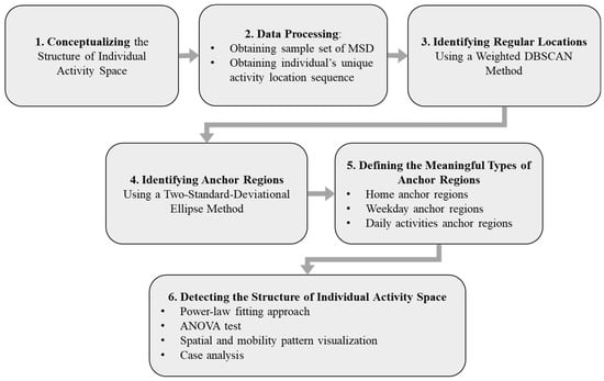
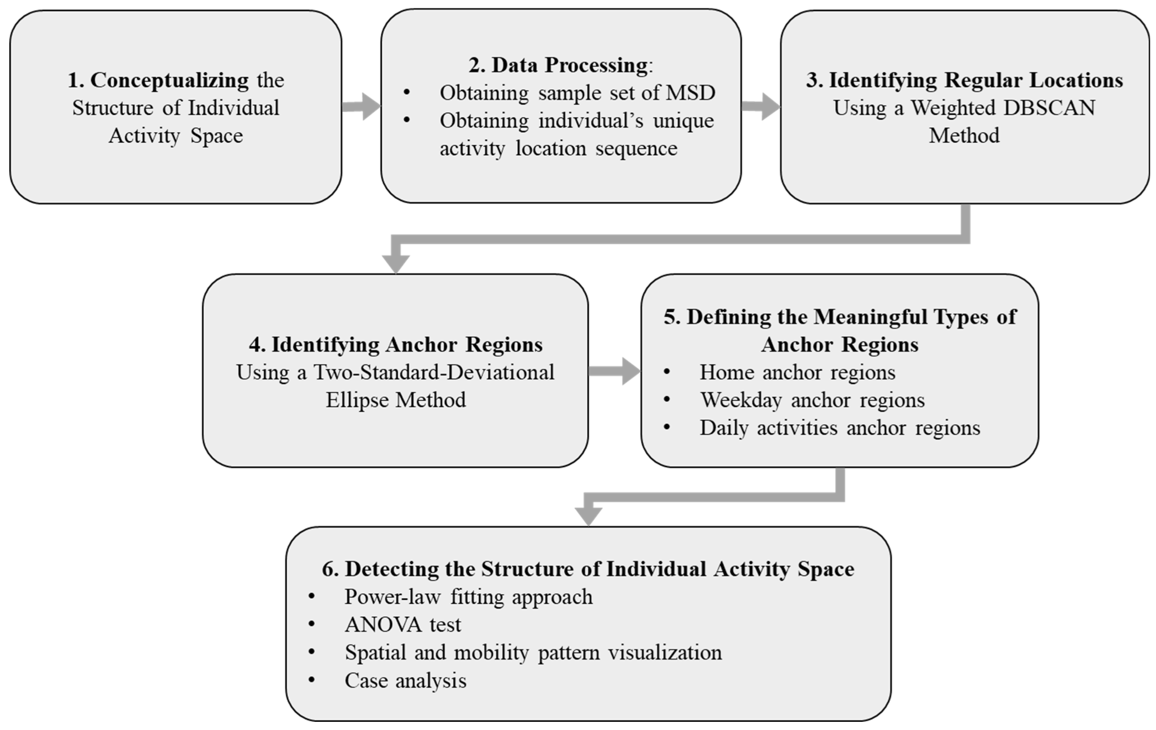
This study develops a comprehensive framework for analyzing individual activity space structure using mobile signaling data. The methodology comprises six main stages, as illustrated in Figure 1. First, we conceptualized activity space into five core elements. Second, we collected three-month mobile signaling data records of permanent residents in Shenzhen, and preprocessed the data to extract individual-level stay records of 10,848 representative samples. Third, we applied a weighted DBSCAN clustering algorithm to identify regular locations, with parameters optimized through k-distance analysis. Fourth, we used the two-standard-deviational ellipse (2SDE) method to define anchor regions and potential activity spaces. Fifth, we classified the anchor regions into three functional types. Finally, we analyzed the structure of individual activity space through power-law fitting, analysis of variance (ANOVA) tests, and specialized visualization techniques. This integrated approach enables a multi-dimensional examination of both the hierarchical organization and spatial characteristics of human activity patterns.
Figure 1.
Technical roadmap.
2.2. Conceptualizing the Structure of Individual Activity Space
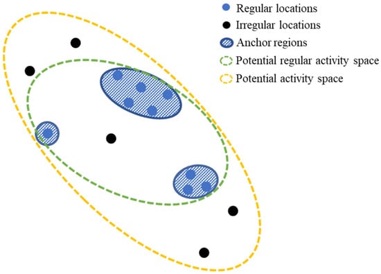
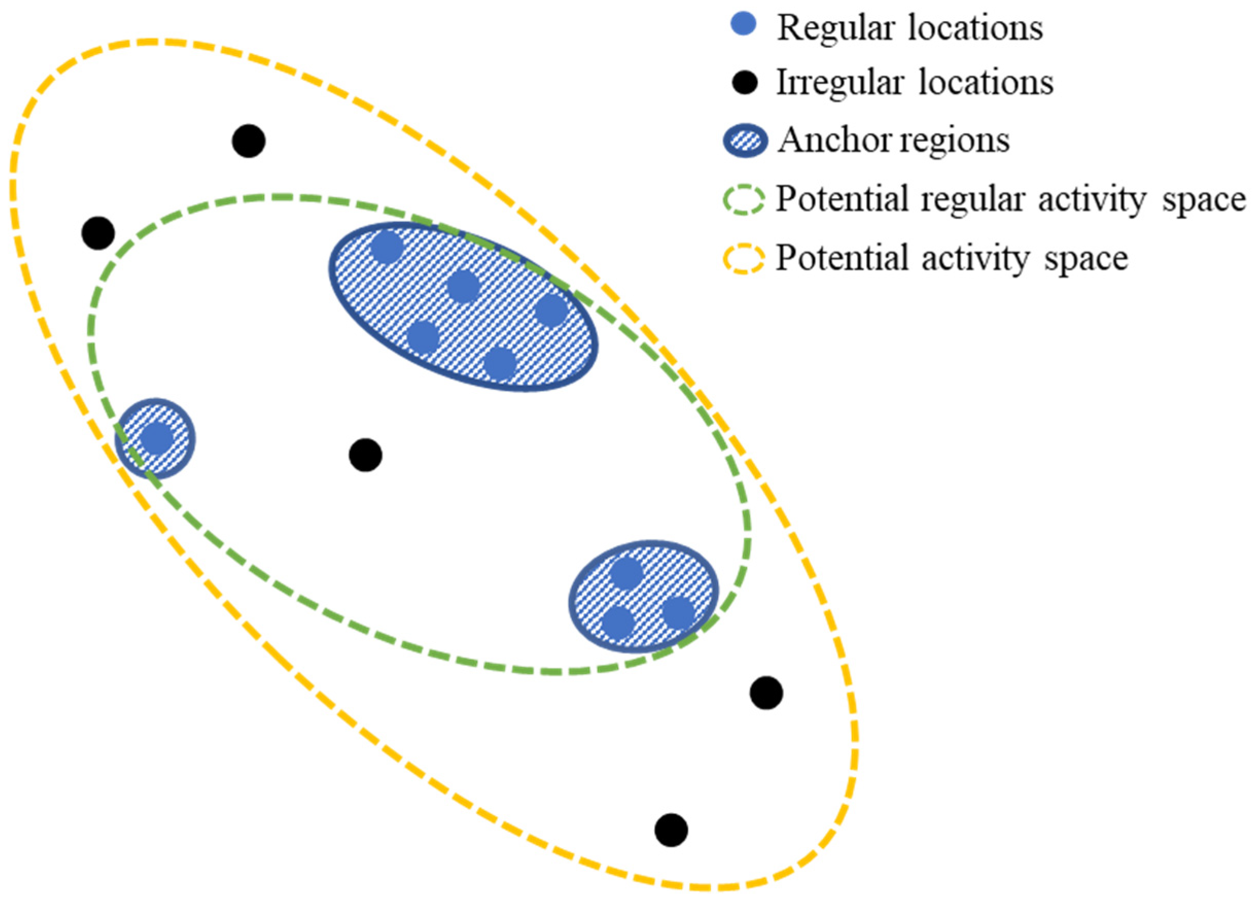
We conceptualized the spatial structure of an individual’s activity space with 5 fundamental elements (Figure 2), as follows:
Figure 2.
The conceptual structure of an individual’s activity space. Note: The structures depicted are conceptual archetypes used to guide the rule-based classification. Real-world patterns may form a continuum or include hybrid cases (e.g., work-from-home scenarios merging home and work anchors), which are accounted for in the empirical classification based on an individual’s actual anchor regions.
- (1)
- Regular locations (RLs): Point-based locations that an individual regularly visits, usually defining by the total time spent or the frequency of visit. Often presented in groups.
- (2)
- Irregular locations (IRLs): Point-based locations that an individual occasionally visits, with less time spent and lower frequency of visit than the regular locations. Often scattered distribution.
- (3)
- Anchor regions (ARs): Region-based places formed by either groups of regular locations or a single regular location and the vicinity of these/this location(s), suggesting the actual activity space that often has significant meanings for an individual’s everyday life.
- (4)
- Potential regular activity space (PRAS): The spatial extent derived from all regular locations. It represents the area within which an individual is likely to move between their regular, frequently visited anchor regions, reflecting their routine accessibility in daily life.
- (5)
- Potential activity space (PAS): The spatial extent derived from all visited locations (both regular and irregular). It captures the maximum area an individual could potentially encounter or traverse during their daily travel, thus representing their overall accessibility.
As shown in Figure 2, an individual’s activity space has a complex internal structure, with anchor regions being the essential part, as well as the subcenters. In the following sections, we focus on precisely detecting the individual’s anchor regions as well as the structural patterns. We also detect the two potential spaces, and statistically compare their spatial attributes with that of the anchor regions.
2.3. Data Processing
2.3.1. Study Area and Mobile Signaling Dataset
This study uses Shenzhen as a case—a major high-density city in southern China, adjacent to Hong Kong, covering 1952 km2 with a population of 13.44 million in 2019 [49]. Analyzing residents’ anchor regions helps understand activity space structure in large Chinese cities.
We employed three-month continuous individual-level mobile signaling data (MSD) of Shenzhen from 8 October 2019 to 31 December 2019 (the influence of the National Day holiday is excluded), collected by China Unicom Company, one of the three cellular operators in China. The dataset covers mobility trajectory records with fine-grained spatial and temporal resolutions of over 17 million mobile phone users. Locations were recorded at the base-station level (around 250 m resolution) when users made calls, used apps, or stayed in a cell for over 30 min. The dataset includes trip sequences with origin–destination coordinates, start and end times (1 min resolution), speed, distance, and socioeconomic attributes. Compared to traditional CDR, MSD offers richer, denser records with finer spatiotemporal granularity [24,25].
To focus on permanent residents, we followed the following steps:
- (1)
- Selected the mobile phone users who stayed no less than 15 days per month in the city and had at least 15 trips per month;
- (2)
- Removed the users who do not have a stable home location. Specifically, exclude those whose home locations identified in each month differ by more than 500 m;
- (3)
- Crawled the boundaries of 3109 neighborhoods in Shenzhen through Baidu API (https://lbsyun.baidu.com/ (accessed on 1 November 2019)), and selected the users whose home locations fell into the neighborhoods which contained at least 9 other users.
We also excluded the trip records with significant errors, such as ping-pong effect, data drifting, and missing displacement.
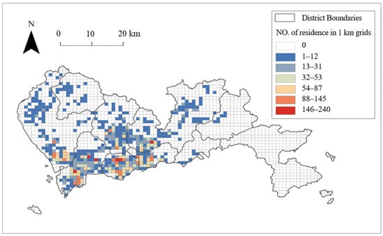
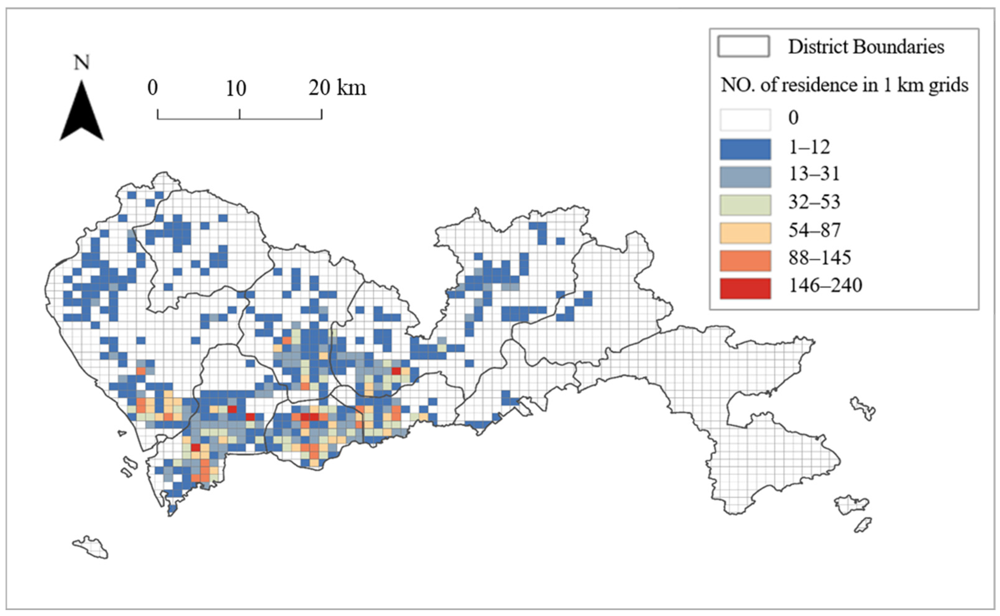
Finally, we obtained over 2.56 million trip records from 10,848 mobile phone users, whose addresses are distributed in 576 neighborhoods in Shenzhen (Figure 3). On average, each sample has 21 days of trip records per month and around 236 activities (max = 526; min = 109) distributed in around 39 locations (max = 213; min = 6) during the three months. The signaling sample data used in this study cover the major urbanized areas of Shenzhen, with a large and temporally continuous sample, allowing for robust representation of the city’s mobility structure. Although communication frequency differs across user groups, the data provider conducted random sampling and anonymization prior to release, ensuring that the dataset remains statistically representative at the aggregate level.
Figure 3.
Study area with distribution of sample residence based on 1 km grid.
2.3.2. Obtaining Individuals’ Unique Activity Location Sequence
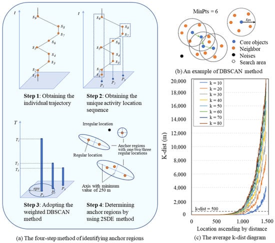
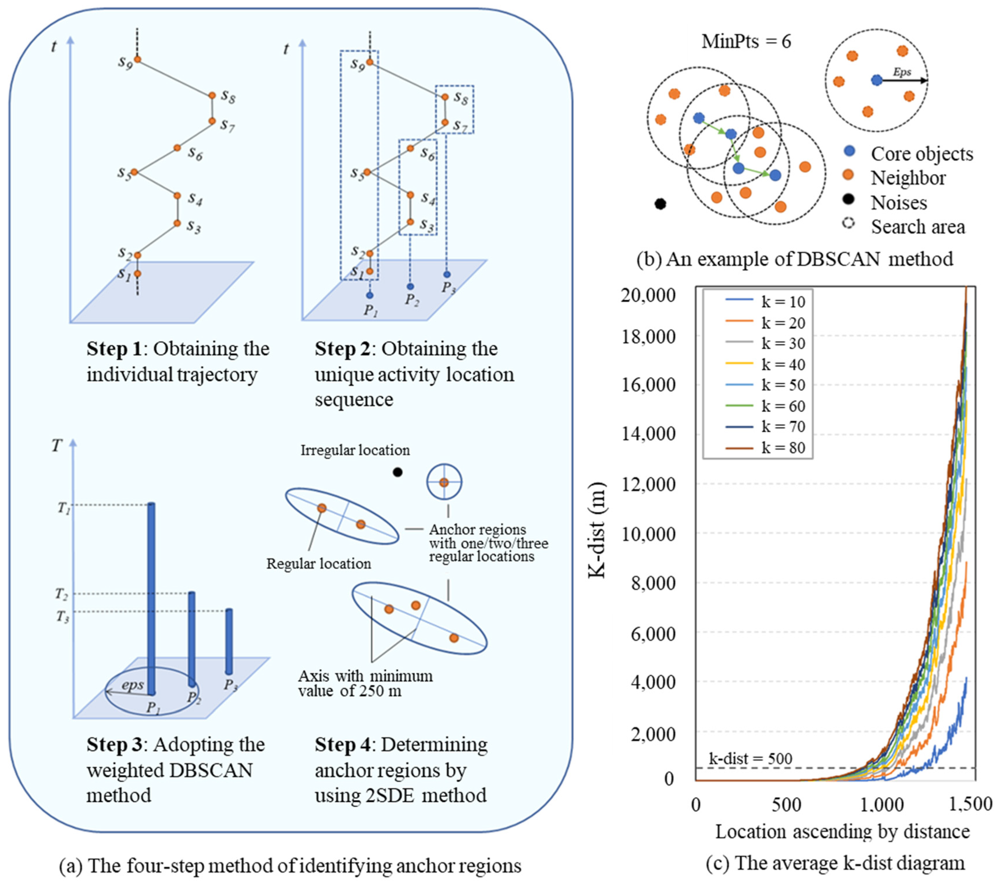
From the raw trip sequence record, we derive an individual’s trajectory set as a chronological sequence of stay records following two steps (Figure 4a):
Figure 4.
Anchor region detecting methods and the tuning process.
First, we obtained an individual’s mobile phone trajectory T from the trip sequence record. The trajectory is derived as
where denotes the i-th stay record during the three-month period (in chronological order); and represent the longitude and latitude of the base station to which the individual is assigned.
Second, we combined the stays which have the same longitude and latitude to obtain an individual’s unique activity location sequence , which can be derived as
where denotes the i-th unique activity location record during the three-month period; and represent the longitude and latitude of the assigned base station; is the duration of stay in such location.
2.4. Identifying Regular Locations Using a Weighted DBSCAN Clustering Method
We employ a weighted DBSCAN algorithm to cluster regular locations and identify anchor regions based on the individual-level activity location sequences we built in the former steps. DBSCAN is chosen for its merits in detecting arbitrarily shaped clusters without pre-specifying their number, and to classify low-density points as noise (i.e., irregular locations). The algorithm requires two parameters: Eps (search radius) and MinPts (minimum number of points within Eps, as shown as Figure 4b).
To incorporate temporal significance, each stay point is assigned a normalized weight based on its total time spent. This weighting scheme effectively adjusts local density estimates during clustering, ensuring that locations with longer dwell times are more likely to be identified as core points. The approach is conceptually equivalent to replicating points proportionally to their time weights, maintaining full compatibility with the original DBSCAN framework [45,48]. Recent studies have validated the use of temporally weighted DBSCAN for detecting activity anchors in large-scale mobility datasets [45,46]. Notably, a single point with sufficiently high accumulated weight (from repeated or prolonged visits) can satisfy the core condition and form its own cluster, effectively preserving meaningful “loner” locations that function as important activity anchors. This property ensures that spatially isolated—yet behaviorally significant—hubs (such as a major transit station visited intensively by an individual) are not overlooked.
The chosen parameters (Eps = 500 m; MinPts = 50) were based on both the k-distance method (Figure 4c) [48]. We calculated the distance from each point to its k-th nearest neighbor with k values tested between 40 and 80, corresponding to 40–80 cumulative hours over three months. The analysis revealed a clear inflection point at 500 m, with stability achieved when k was no smaller than 50. We tested several nearby combinations and found that the overall number and spatial hierarchy of anchor regions remained stable, indicating that the results are not sensitive to small parameter changes. Therefore, only the representative setting is reported for clarity.
The algorithm outputs were interpreted as follows: clusters of core and border points were classified as regular locations and grouped into anchor regions, while noise points were designated as irregular locations.
To examine the sensitivity of our findings to the definition of a regular location, we also performed a comparative analysis using frequency-weighted DBSCAN, where each point was weighted by its visit count instead of total time spent. This alternative approach shifts the focus from temporal investment to visit repetition, offering a complementary perspective on regular locations. A comparative analysis of both methods is provided in Appendix A.
2.5. Identifying Anchor Regions Using a Two-Standard-Deviational Ellipse Method
Each cluster of regular locations is delineated using a two-standard-deviational ellipse (2SDE), which captures the spatial dispersion and orientation of points while containing approximately 95% of locations. The 2SDE method is widely adopted in activity space studies for its interpretability and comparability [6,27]. The construction of anchor regions using 2SDE has an underlying assumption that the individual knows and is actually exposed to all of the places covered by the ellipse. For clusters with only one regular location, a circular buffer of a 250 m radius (matching data resolution) is used.
We further measured the potential regular activity space and potential activity space for comparison by also using the 2SDE. Potential regular activity space is based on all regular locations, representing areas frequently visited or traversed. Potential activity space is based on all (regular and irregular) locations, representing the full extent of an individual’s spatial exposure. In contrast to the anchor regions, the underlying assumption of the two measured potential spaces is that all of the places covered by the ellipse are known and have possibly been visited by an individual.
The two-standard-deviational-ellipse (2SDE) method was adopted primarily for its interpretability and comparability with previous studies. While other shape-based methods such as α-shapes or kernel density contours can offer finer geometric precision, 2SDE provides a clear indication of spatial dispersion and directional tendency. Minor exaggeration of elongated shapes may occur but does not affect the overall spatial hierarchy or analytical conclusions [47].
It is important to note that the potential activity space, derived from the 2SDE of all visited locations, serves as a geometric descriptor of the maximum spatial extent of an individual’s daily travels. This is a simplified representation of the theoretical spatial footprint. It does not imply a uniform probability of visiting all areas within the ellipse, particularly as the inclusion of rarely visited, distant locations (e.g., an airport) can disproportionately stretch its boundaries. In this study, this measure is used primarily as a comparative metric to contrast against the much more concentrated area of actual, regularly visited anchor regions, rather than as a literal surface of visitation likelihood.
2.6. Defining the Meaningful Types of Anchor Regions
We classified anchor regions into three types based on visitation patterns, as follows:
- Home Anchor Region (HAR): An everyday anchor region, at which the probable vicinity around an individual’s home is determined. We defined it as the anchor region in which an individual spends most time. The underlying assumption of our definition is that places around home play the most vital role in an individual’s daily movement [2].
- Weekday Anchor Region (WAR): A weekday-focused anchor region, at which the probable vicinity around an individual’s workplace is determined. For non-home anchor regions, we defined a weekday anchor region as the anchor in which an individual spends no less than 3 h per weekday and in which no less than 70% of time spent is on weekdays. The threshold was chosen after multiple trials balancing differentiation and interpretability. This value aligns with thresholds commonly used in home–work location detection in similar activity-mobility studies [27,39]. We clarify that this indicator does not necessarily identify formal workplaces but rather denotes the primary weekday activity center of an individual.
- Daily Activity Anchor Region (DAR): A regularly visited anchor region, at which the major regions of regular daily activities are determined. All of the anchor regions apart from the home and weekday anchor regions are defined as daily activity anchor regions.
2.7. Detecting the Structure of Individual Activity Space
2.7.1. Power-Law Fitting Approach
We applied power-law fitting to characterize the heavy-tailed distributions observed in the hierarchy of anchor regions. Specifically, we ranked each individual’s anchor regions by total time spent and visit frequency; then, we tested the relationship between the rank and these metrics. The fit was performed using a standard power-law function of the form , where x represents the rank of the anchor region. The parameters a (the scaling factor) and b (the exponent) were estimated to characterize the concentration of activities. Given the large sample size, the log–log linearity of the tail distribution is sufficient to indicate a power-law tendency. Although a more rigorous maximum-likelihood estimation could be applied, it would not alter the qualitative interpretation of the results [50].
2.7.2. ANOVA Tests
To compare spatial metrics across different activity space structures, we conducted one-way analysis of variance (ANOVA) followed by post hoc multiple comparisons. Variables, including the size of potential activity space, potential regular activity space, total anchor region size, and average anchor region size, were tested for normality prior to ANOVA. Despite mild skewness in some indicators, the large sample size (n > 10,000) ensured the robustness of the ANOVA results. Significant differences (p < 0.05) between structure types were further visualized using letter-based notation.
2.7.3. Spatial and Mobility Pattern Visualization
We developed several visualization techniques to illustrate the composition and mobility patterns of activity space structures. First, spatial diagrams of the six major activity space structures were generated, each accompanied by a typical example. Second, chord diagrams were used to represent trip flows between and within anchor regions, highlighting the dominance of intra-anchor region mobility. Third, boxplots with statistical annotations display the results of multiple comparisons for spatial metrics across different structural types. These methods collectively allowed for a multi-dimensional assessment of the size, structure, and mobility patterns inherent in individuals’ activity spaces.
3. Results
3.1. The Exploration of Anchor Regions and Their Hierarchy Characteristics
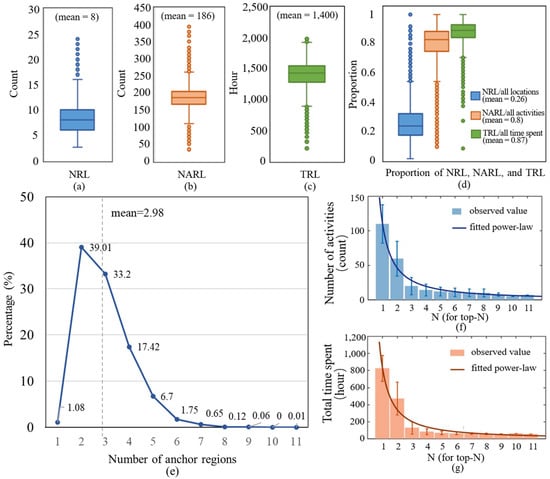
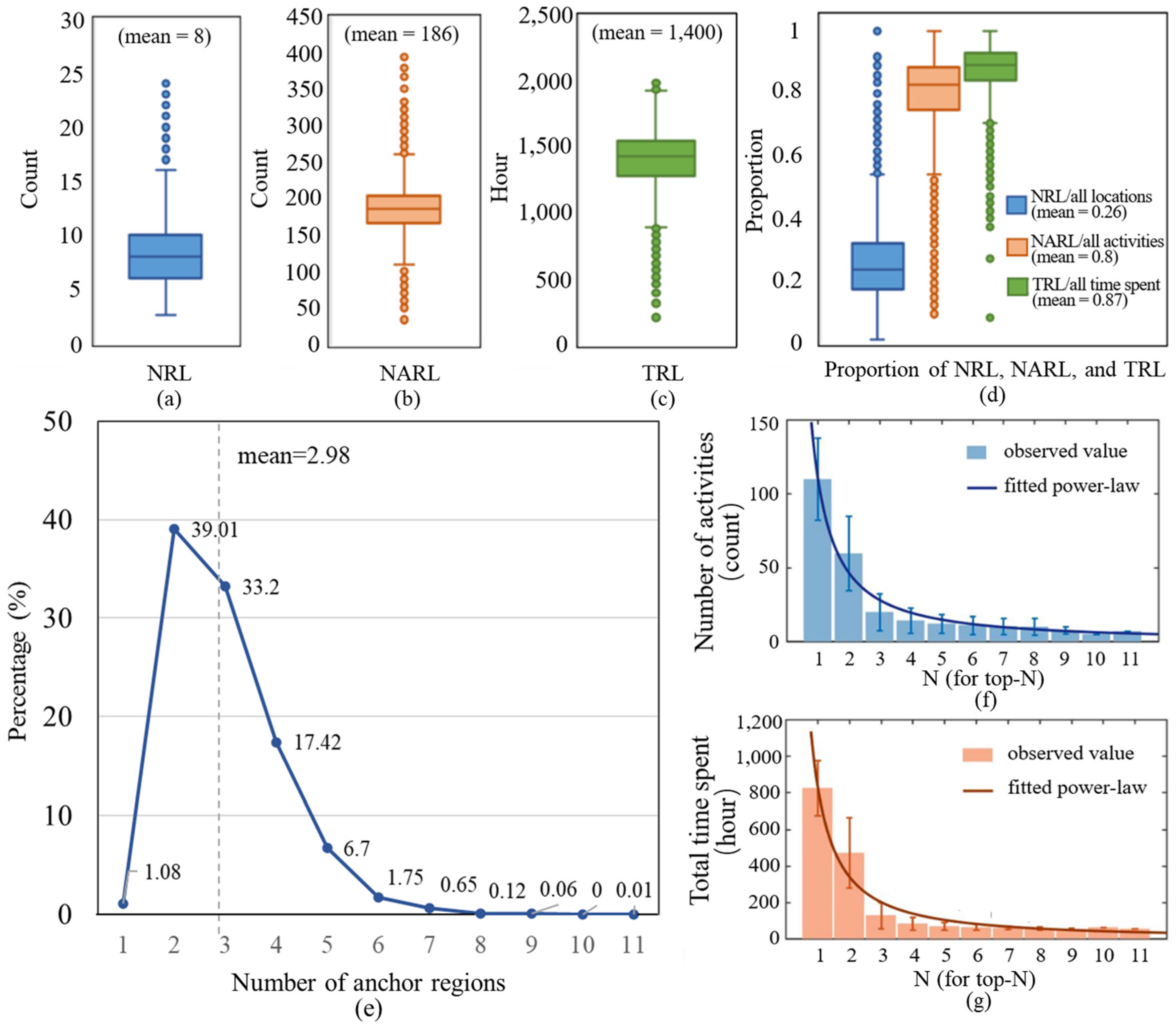
By applying the weighted DBSCAN method to the location sequences of 10,848 individuals, we derived basic statistics on regular activities (Figure 5a–d). On average, only 26% of all locations visited by an individual were classified as regular locations; however, these accounted for 80% of all activities and 87% of total time spent. Specifically, the average individual had eight regular locations, which hosted 186 activities (approximately 2 per day) and accumulated 1400 h of dwell time (about 16 h per day). This pronounced concentration of time and activity in a small subset of places strongly reaffirms the high regularity of human spatiotemporal behavior [26,51,52].
Figure 5.
Distribution of the statistics for regular locations and anchor regions, including (a) Number of regular locations (NRL) per person; (b) Number of activities in regular locations (NARL) per person; (c) Total time spent in regular locations (TRL) per person; (d) Proportion of NRL, NARL and TRL to all locations, all activities and all time spent per person; (e) Distribution of the number of anchor regions; (f) Number of activities in top-Nth anchor regions; (g) Total time spent in top-Nth anchor regions. Note: The sample sizes of top-Nth anchor regions in (f,g) are 10,848, 10,731, 6499, 2898, 1008, 281, 91, 20, 7, 1, 1 (arranged in ascending order according to the value of N).
We further found that an individual’s regular locations are grouped into small sets of clusters, which form the anchor regions as defined by our study. The average number of anchor regions for an individual is 3, and the minimum and the maximum number of anchor regions is 1 and 11, respectively (Figure 5e). Notably, 95% of people possess no more than five anchor regions. The distribution of the number of anchor regions is consistent with the limited diffusivity commonly observed in human mobility [53]. These findings indicate that activity space is organized around a small set of key nodes.
Time utilization across anchor regions exhibits a heavy-tailed distribution (Figure 5c). In Figure 5f,g, we ranked the anchor regions of each person by total time spent and generate n types of clusters, denoted as top-Nth anchor regions (where n equals the number of anchor regions the individual has). Then, we calculated the average of total time spent and the number of visits (activities) in each of the top-Nth anchor regions for all individuals. Note that the statistics of each top-Nth anchor region is based on different totality. When ranked by total time spent, both the duration and number of visits in these ranked anchor regions follow a power law (a power-law distribution is derived as ; for the average total time spent measure, a = 847.2 and b = −1.3; for the average number of visit measure, a = 112.1 and b = −1.3) (r-square = 0.95 and 0.97, respectively), indicating that a majority of time and visits are concentrated in the top-ranked anchor regions. This aligns with the Pareto principle, a common pattern in human mobility [54,55].
Furthermore, a clear hierarchy exists among anchor regions when estimating the time utilization of the top-Ns. As shown in Figure 5c, the top-ranked region accounts for 825 h (9.7 h/day) and 110 visits (1.8/day), consistent with a “home” anchor. The second and third regions (5.5 h/day and 1.5 h/day, respectively) function as daily anchors, like workplaces, while lower-ranked regions (each <1 h/day) act as weekly leisure anchors. This temporal hierarchy validates our functional classification of anchor regions.
Notably, we conducted a comparative analysis of duration-weighted and frequency-weighted DBSCAN to examine how different conceptualizations of regular locations in-fluence the derived structure of activity spaces (see Appendix A). The results indicate that frequency weighting tends to identify a larger number of fine-grained anchor regions, which often correspond to short-duration, high-frequency stops. In contrast, duration weighting yields fewer, more dominant clusters that better reflect core life anchors, such as the home and workplace. This distinction underscores that parameter selection embodies a conceptual trade-off between capturing the richness of visit repetition and delineating the hierarchy of temporal investment in urban space.
3.2. The Comparison of Individual Actual and Potential Activity Space
We estimated the spatial extent of the potential activity space, potential regular activity space, and anchor regions by constructing two-standard-deviation ellipses (2SDEs) for all locations, regular locations, and each anchor region (Table 1). The sizes of the potential regular activity space and the anchor regions (both total and average) follow a left-skewed distribution, indicating a prevalence of small spatial extents. This finding is consistent with the heavy-tailed distributions of regularly visited activity spaces reported in previous studies [26,54]. In contrast, the size of the potential activity space approximates a normal distribution. This divergence highlights the more concentrated spatial pattern of an individual’s regularly visited places.
Table 1.
Comparative statistics of actual and potential activity space.
As shown in Table 1, an individual’s anchor region contains approximately three unique locations on average, covering about 0.1 to 0.2 km2 (comparable to a 315–450 m grid or a 180–250 m radius circle). The combined size of all anchor regions for an individual typically ranges from 0.2 to 0.5 km2 (equivalent to a 450–700 m grid or a 250–400 m radius circle). These metrics delineate the limited spatial extent of an individual’s actual activity space—the area they are regularly exposed to in daily life.
The potential regular activity space ranges mainly from 4 to 53.7 km2, suggesting variation in individual daily accessibility. In comparison, the median size of the overall potential activity space is about 594.2 km2, which is approximately 50 times larger than that of the potential regular activity space (based on the 50% percentile). This substantial disparity underscores the critical importance of measuring actual, rather than potential, activity spaces.
3.3. The Inner Structure of Individual Activity Space
After defining meaningful anchor region types (see Section 2.6), we analyzed the composition of each individual’s anchor regions to differentiate the internal structure of their activity space. This section summarizes typical activity space structures and compares their spatial and mobility patterns both within and between anchor regions, namely, intra- and inter-anchor region mobility patterns.
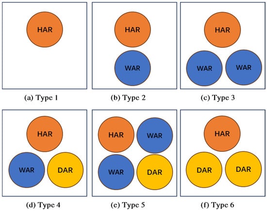
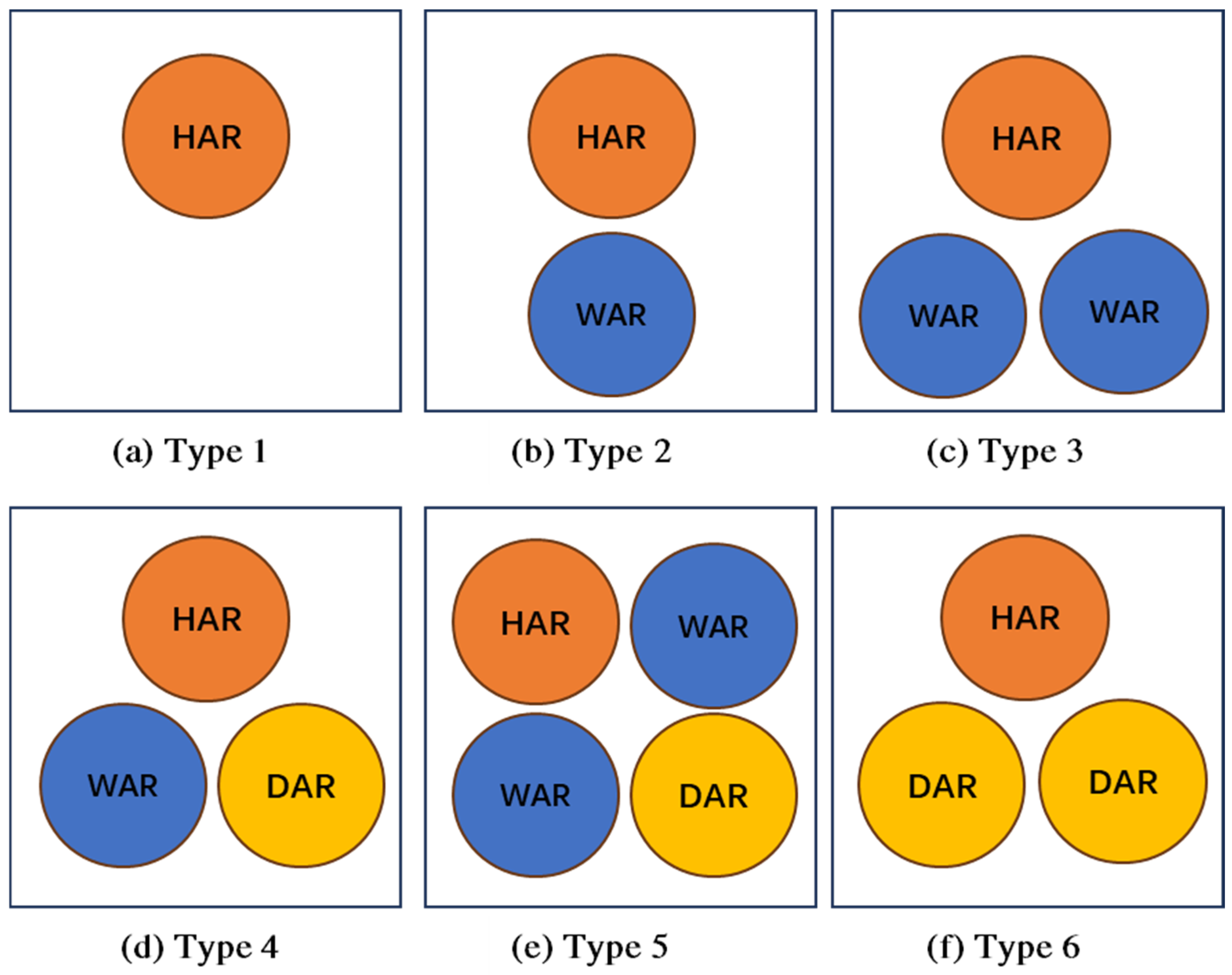
As outlined in Table 2, all individuals have one home anchor region. The number of weekday anchor regions ranges from 0 to 3, and daily activity anchor regions range from 0 to 10. To classify activity space types, we first grouped individuals by the number of weekday anchor regions—reflecting regular weekday spatiotemporal patterns. Those with one weekday anchor region likely have a fixed primary location (e.g., a full-time job), while those with multiple may have several workplaces or regularly visited sites. Individuals with no weekday anchor region may be freelancers or work from home. We further subdivided each group based on the presence of daily activity anchor regions, and this division distinguishes non-necessary activity patterns. Overall, we summarized six major activity space types. Two additional rare types with no irregular locations were derived but excluded from further analysis due to the small sample size (n = 3).
Table 2.
Structural composition of individual activity space.
As Figure 6 shows, Type 1 exhibits a monocentric structure centered on a home anchor region, accompanied by multiple irregular locations; it is the least common, comprising only 1% of the sample (Table 2). Types 2 and 4 are predominant among employed individuals, with Type 4 showing greater spatial diversity beyond workplace-related anchors. Types 3 and 5, though less frequent, reflect polycentric patterns characterized by multiple weekday anchor regions. Type 6 incorporates both home and daily activity anchor regions and contains the highest number of daily activity anchors, indicating the most diverse set of regularly visited destinations.
Figure 6.
The composition of anchors within six major types of structures.
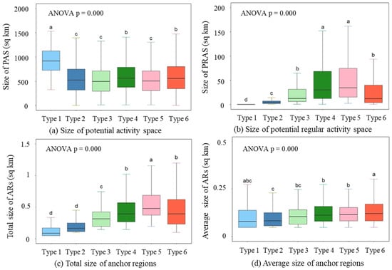
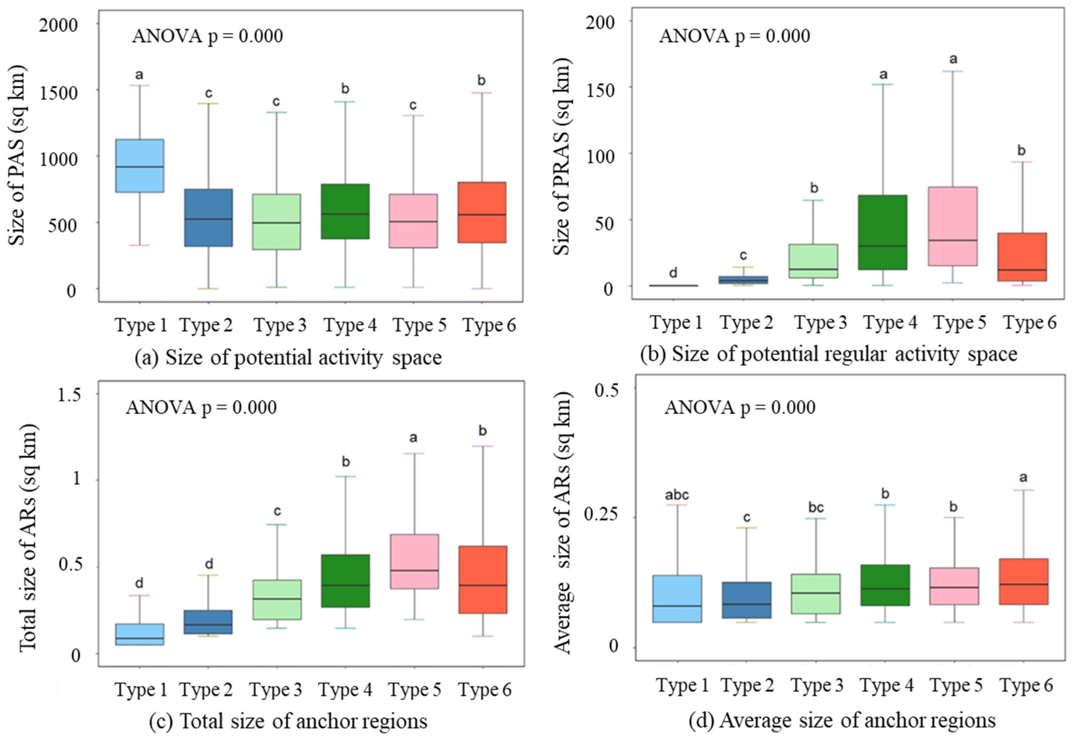
To compare spatial patterns across the six major structure types, we performed ANOVA tests on the sizes of both actual and potential activity spaces, followed by multiple comparison analysis. Four size measures were used: the size of the potential activity space, potential regular activity space, total anchor region, and average anchor region size. All measures met normality assumptions (significance level: 0.1 for potential regular activity space; 0.05 for others). Each measure varied significantly among the six types (p = 0.000). Multiple comparison results are indicated by letter-based groupings: types not sharing the same letter differ significantly in the corresponding measure (Figure 7).
Figure 7.
The multiple comparison results of the actual and potential activity spaces.
Types with more daily activity anchor regions (Types 4, 5, and 6) have significantly larger average anchor region sizes, while Type 2 has the smallest. This suggests that individuals with diverse anchor regions also occupy broader vicinities around each regular destination. Types combining weekday and daily activity anchors (Types 4 and 5) exhibited the largest potential regular activity spaces, whereas Type 1 had the smallest—consistent with the intuition that traveling between diverse anchor regions increases geographical exposure. Interestingly, Type 1 also showed the largest potential activity space, indicating high randomness in this monocentric structure. Conversely, smaller potential activity spaces in other types reflect the capacity of anchor regions to capture longer-distance travel.
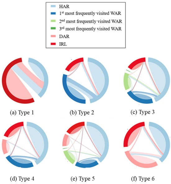
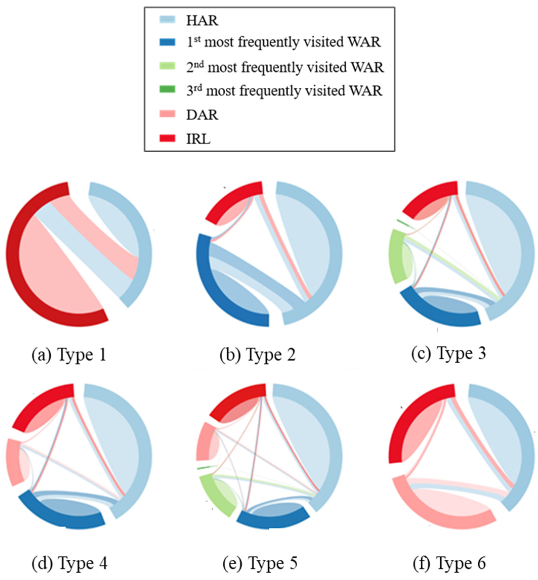
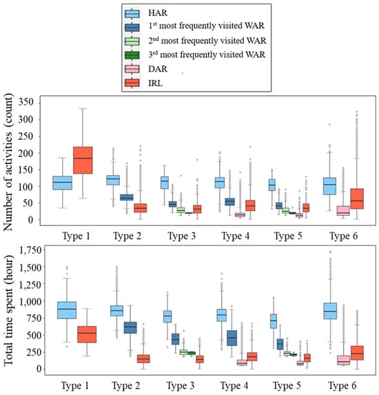
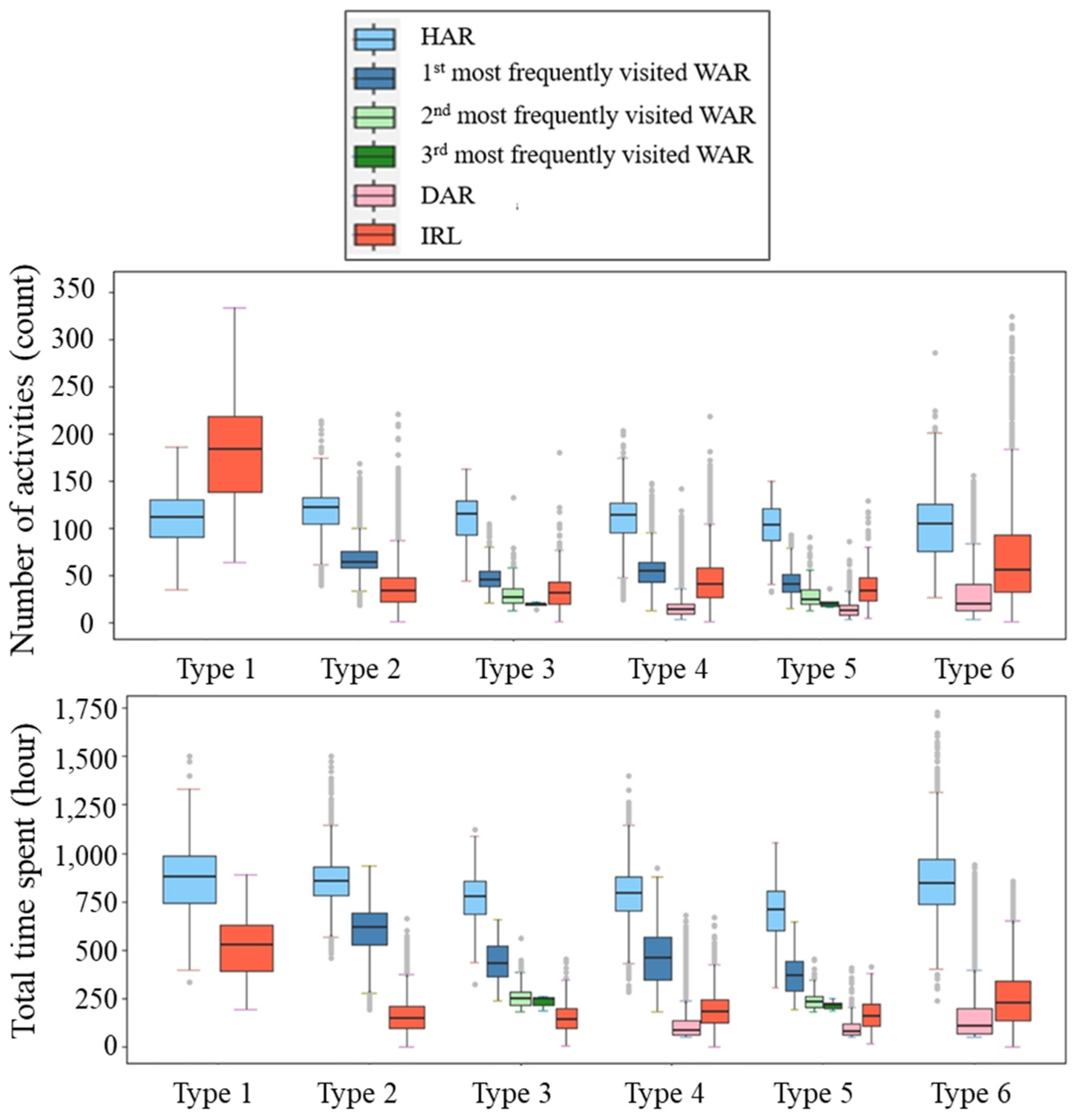
To analyze intra- and inter-anchor region mobility across activity space structures, we calculated the average trip distribution (Figure 8) and time utilization per anchor region type (Figure 9). Results show that most trips occur within—not between—anchor regions, underscoring their role in capturing daily movement and the importance of short-distance trips over long commutes. This suggests that enhancing local accessibility and sustainable mobility within anchor regions would be a priority in urban planning.
Figure 8.
The intra- and inter-anchor region mobility patterns of 6 typical structures.
Figure 9.
Temporal utilization of 6 typical structures.
Time-use analysis reveals the home as the dominant anchor region across all six structure types, with both the highest time spent and number of visits among all types of anchor regions. In Types 2–5, weekday anchor regions also function as a key center area, with time spent only slightly lower than at home, indicating bicentric or polycentric activity patterns. These findings call for expanding home-centered planning to a multi-anchor, context-sensitive approach.
3.4. Case Analysis: Illustrative Examples of Activity Space Structures
To further understand the characteristics of different activity space structures within real geographic contexts, we present four illustrative cases.
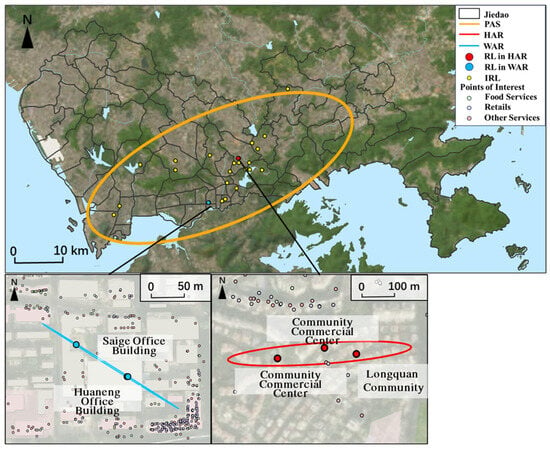
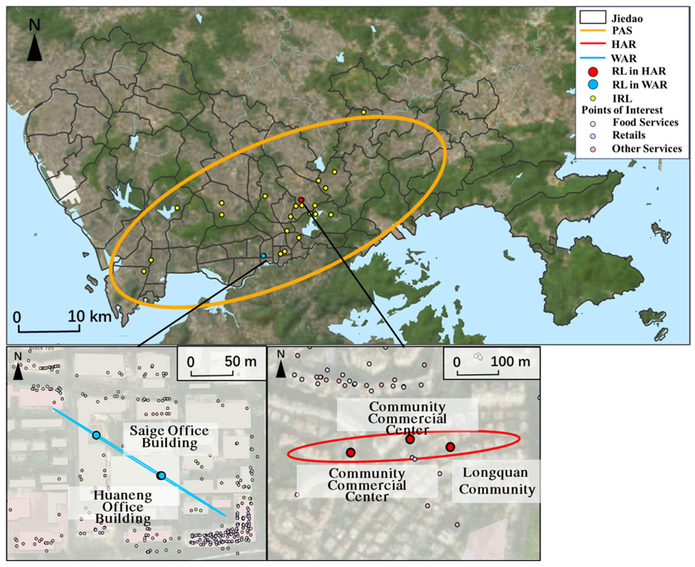
Among individuals with regular weekday destinations, we selected two representative cases (Figure 10 and Figure 11). Figure 10 illustrates the Type 2 structure of a 55–59-year-old female, characterized by a classic dual-core spatial pattern. The home anchor region (HAR) is tightly centered on the Longquan Community, a residential area, with its regular locations clustered around local commercial facilities, indicating a home-centered living circle. In clear spatial division, the weekday anchor region (WAR) is distinctly located within the Huaqiangbei district, a major employment hub. This clear geographic separation between a defined residential community and a busy job center visually underscores a stable, commute-oriented lifestyle typical of formal employment.
Figure 10.
A case of Type 2 structure, with a home anchor region and a weekday anchor region.
Figure 11.
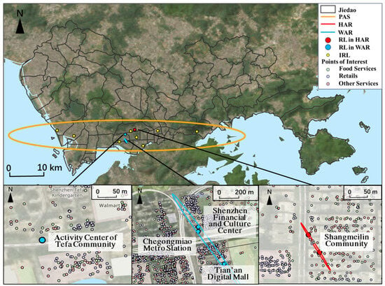
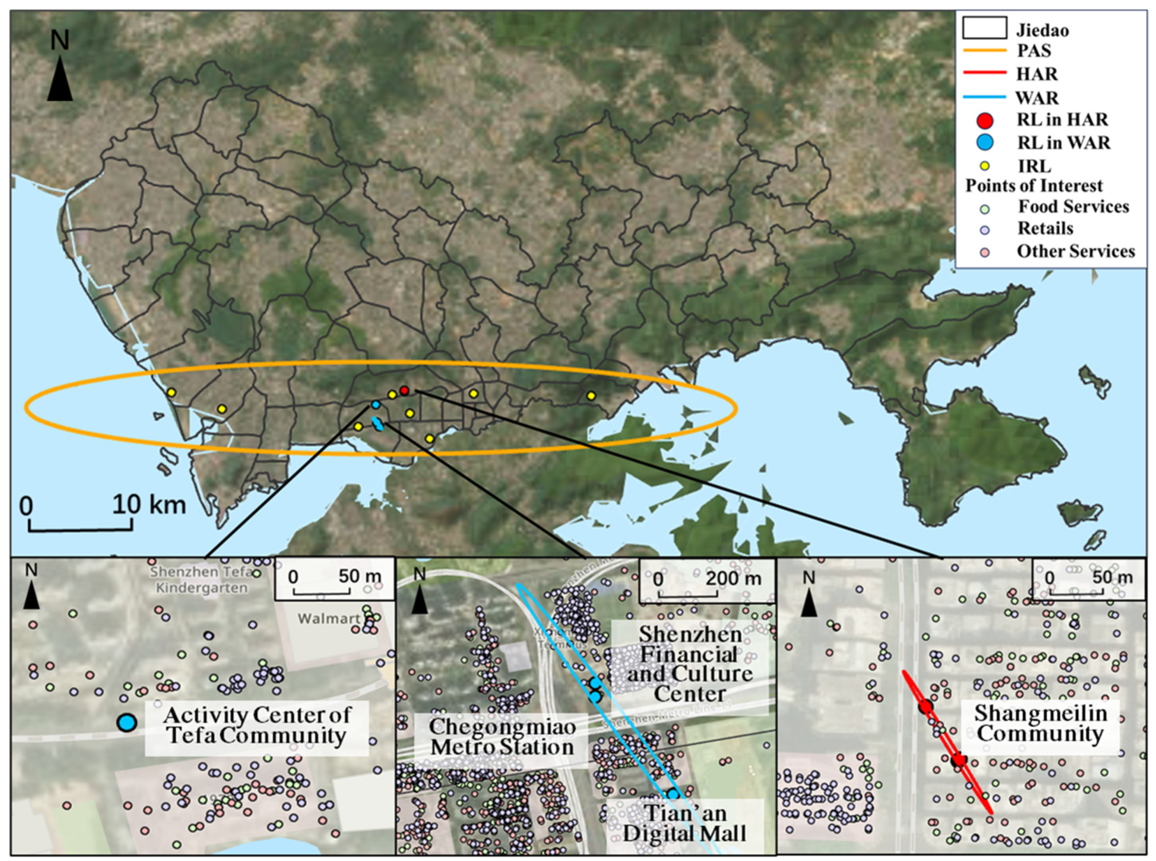
A case of Type 3 structure, with a home anchor region and two weekday anchor regions.
In contrast, Figure 11 illustrates the Type 3 structure of a 25–29-year-old male, showcasing a polycentric but tightly structured routine. It features multiple, clustered weekday anchor regions around the Chegongmiao Metro Station, indicating employment in a dense, multi-nodal business district, alongside a secondary anchor region around Tefa Community Activity Center, where he spends significant daily time. Compared to the Type 2 structure, this case exhibits markedly fewer irregular locations and an elongated potential activity space concentrated along the axis between these primary anchors. This spatial pattern suggests a highly predictable and efficient lifestyle, emblematic of a time-optimized urbanite who consolidates work and personal life around key anchor regions, minimizing remote travel.
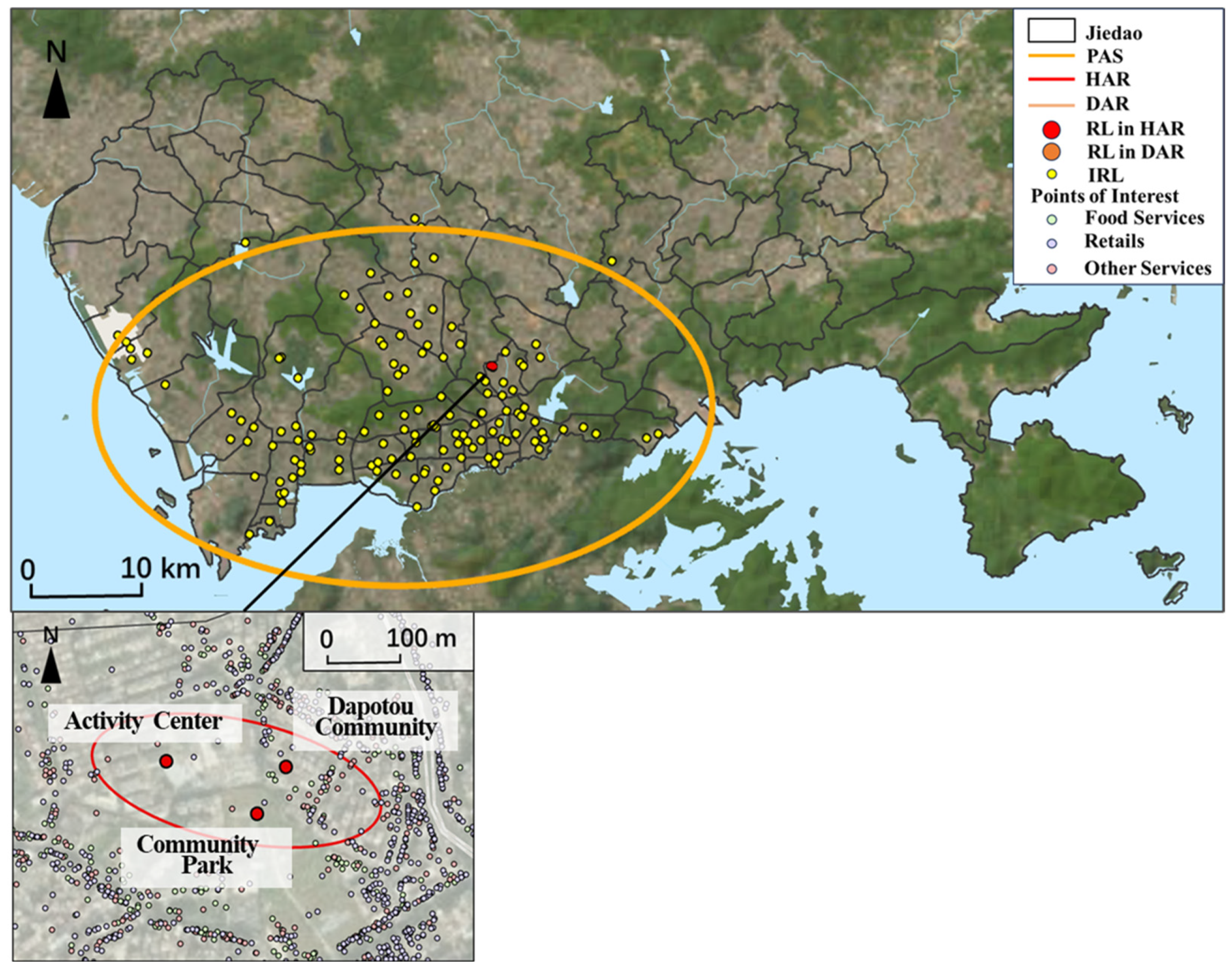
Moving to individuals who lack dominant weekday anchors, Figure 12 depicts the highly localized Type 1 structure of a 55–59-year-old male. His daily activities are almost entirely concentrated within the Dapotou Community, with key regular locations clustered at the community’s Activity Center and the adjacent Community Park. The extremely compact regular activity space and the sparse scattering of irregular locations beyond this core together illustrate a lifestyle deeply rooted in the immediate residential environment. This pattern is strongly indicative of locally oriented life stages, such as retirement or sustained remote work, where daily rhythms revolve around neighborhood-based amenities and social spaces.
Figure 12.
A case of Type 1 structure, with a home anchor region.
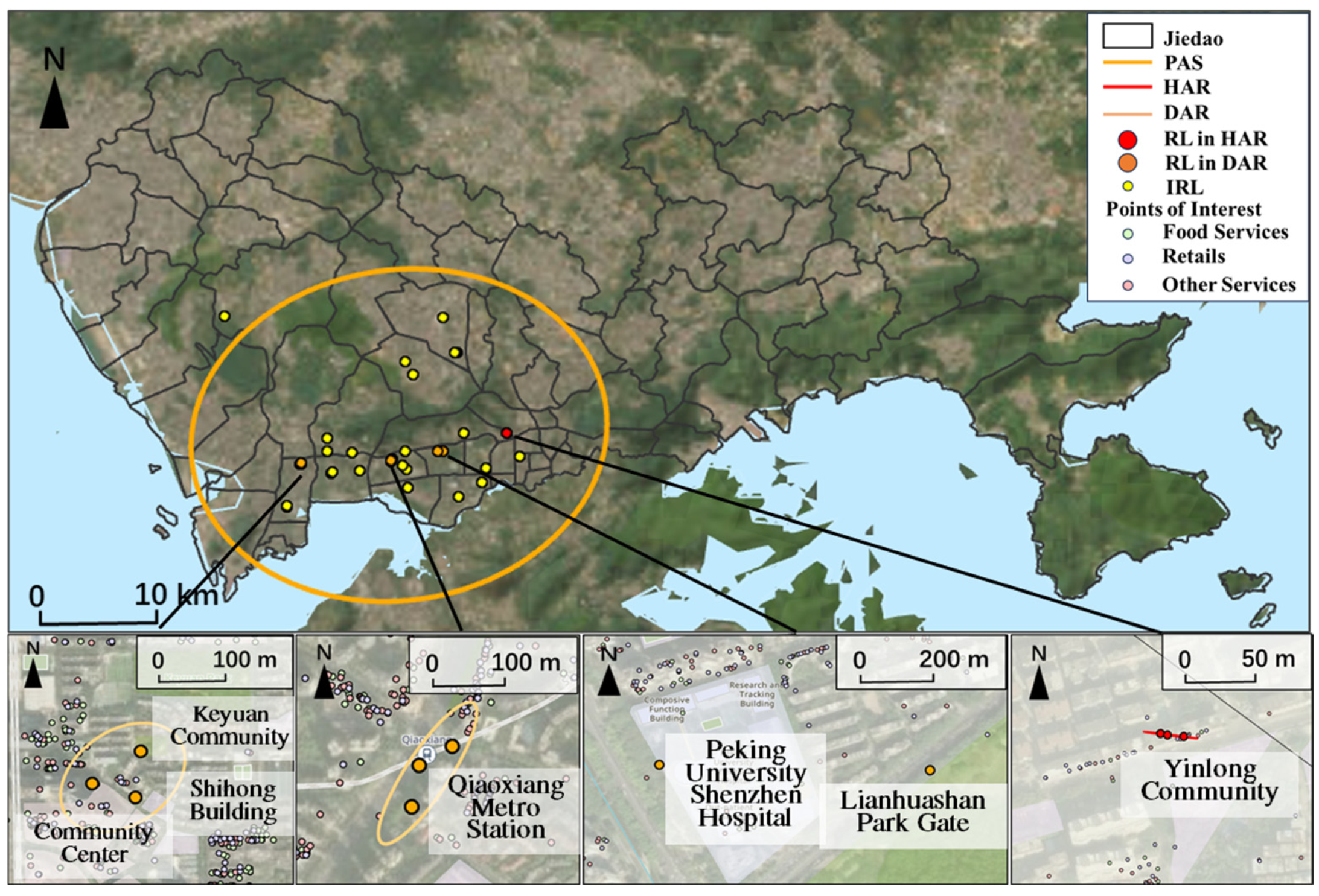
Finally, Figure 13 depicts the spatially complex and diversified Type 6 structure of a 25–29-year-old male. Beyond the home base in Yinlong Community, this individual maintains multiple, geographically scattered daily activity anchor regions (DARs). DARs are anchored to functionally distinct landmarks, including the Qiaongxiang Metro Station (a major transport node), Keyuan Community (possibly for social visits), Peking University Shenzhen Hospital (healthcare), and Lianhuashan Park (recreation). In contrast to the localized, home-centric pattern of Type 1, this structure reflects an outward-oriented, multi-sited lifestyle commonly associated with younger urbanites who actively navigate and integrate diverse functional spaces across the city, balancing personal, social, and service needs within a spatially extensive but structured daily footprint.
Figure 13.
A case of Type 6 structure, with a home anchor region and multiple daily activity anchor regions.
4. Discussion and Conclusions
This study has provided a comprehensive, region-based analysis of the internal structure of individual activity space by leveraging a three-month, high-resolution mobile signaling dataset for 10,848 residents in Shenzhen, China. By using a series of methods, including weighted DBSCAN and two-standard-deviation ellipse, we detected anchor regions and derived the typical structures of activity space based on a rule-based taxonomy. The spatiotemporal patterns of each typical structure were further analyzed. Our findings move beyond traditional point-based conceptions to offer a nuanced understanding of how people cluster their activities in urban space from a region-based perspective. The primary contributions are threefold.
First, our detection of anchor regions substantively extends the anchor point theory proposed by [2]. We empirically demonstrate that individual activity is highly concentrated, with approximately 80% of activities and 87% of time spent within just 26% of all visited locations, which cluster into a limited number of anchor regions (typically no more than five per person). The hierarchical utilization of these regions adheres to a power law, confirming underlying regularities in human mobility [52,53,54,55]. Crucially, we affirm that activity space is polycentric [16,17] but emphasize that each center is a substantive area, not a point. This region-based perspective allows for more precise inference of meaningful locales (e.g., home and work) and their surrounding vicinities, which is vital for uncovering true travel demand.
Second, by comparing the spatial extent of potential activity space, potential regular activity space, and anchor regions, we highlight the critical distinction between theoretical accessibility and actual exposure. The actual area covered by anchor regions is remarkably small (averaging 0.4 km2) and significantly more concentrated than the full potential activity space. This finding provides an empirical measure for actual activity space, offering a more accurate geographic context for studying human–environment interactions.
Third, we defined meaningful anchor region types (e.g., home, weekday, and daily activities) based on behavioral patterns and subsequently categorized individuals into six typical activity space structures following a rule-based taxonomy. The illustrative cases ground these abstract typologies in real urban contexts, exemplified by the dual-core commuter (Type 2), the polycentric time-optimized professional (Type 3), the locally contained neighborhood-centric resident (Type 1), and the multi-anchor network-oriented urbanite (Type 6). These examples show that an anchor region is not merely a statistical cluster but a meaningful geographic container for specific life domains—be it work, home, leisure, or care. This semantic enrichment directly mitigates the Uncertain Geographic Context Problem (UGCoP) by linking behavioral structures to known urban functions [56,57,58].
Another key finding is that intra-anchor region mobility constitutes a fundamental part of daily life, suggesting the anchor region is a more behaviorally relevant geographic unit than administrative boundaries [43]. Furthermore, we found individuals with diverse anchor region types tend to have larger individual anchor regions, while those with more anchor regions often exhibit a more compact potential activity space. These patterns, exemplified by the cases, have direct planning implications. For instance, they can help delineate behaviorally coherent living circles for different social groups—such as designing compact, service-rich neighborhoods for Type 1 individuals, or ensuring efficient transport corridors between key nodes for Type 3 individuals—within frameworks like the 15 min city [44,59]. This framework also holds value for public health, such as identifying primary exposure areas during epidemics [60].
Underpinning these contributions is the use of longitudinal mobile signaling data (MSD). Their fine spatiotemporal granularity and continuous coverage provide a more robust basis for capturing routine mobility compared to cross-sectional surveys or other big data like CDR. This data type holds great potential for further research into social networks, traffic prediction, and equity studies [61,62].
While this study offers significant insights, several limitations should be acknowledged for future research.
First, while 2SDE is a standard and valuable tool for measuring the dispersion of point sets, its application to delineate individual anchor regions requires careful interpretation. It is important to note that fitting an ellipse to a single, dense cluster can lead to an area exaggeration effect, where the derived area is sensitive to the outermost points and may not perfectly represent the compact, intensely used core. The area exaggeration effect also occurs when applying the method to point sets that include rare, far-flung locations. Nevertheless, this methodological characteristic does not undermine our core finding of the extreme spatial concentration of daily life: even with a potential overestimation from 2SDE, the actual area covered by anchor regions (averaging 0.4 km2) remains significantly smaller than the potential activity space. Future research could employ alternative methods, like kernel density estimation or α-shapes, to delineate the core of anchor regions more precisely and compare the results with the 2SDE approach.
Second, a methodological consideration arises from our use of duration-weighted DBSCAN to define anchor regions. While conceptually aligned with our goal of identifying stable, time-intensive cores of daily life, this approach may under-represent the significance of short-duration, regularly visited stops (e.g., airports and post offices) within an individual’s activity space. Our comparative analysis (Appendix A) indicates a conceptual trade-off between the two methods: frequency-weighted DBSCAN identifies more fine-grained regions corresponding to short-duration stops, whereas our duration-based method consolidates these into fewer, dominant clusters centered on major time investments like the home and workplace. Consequently, our operationalization of anchor regions prioritizes temporal dominance over visit frequency. Future work could integrate both perspectives to achieve a more complete depiction of individual activity spaces [31,37].
Third, while this study provides a detailed framework for analyzing individual activity space structures, it primarily operates at the individual level. Future research could scale this analysis by aggregating individuals with similar structure types to examine the socioeconomic profiles, spatiotemporal rhythms, and collective spatial patterns associated with each group. Furthermore, linking these aggregated patterns to urban data (e.g., POI and land use) could reveal how different mobility lifestyles interact with the built environment [32,33,34,35,36]. Such a population-level analysis would enrich the typology and offer nuanced insights for equitable urban planning and service provisions tailored to different behavioral groups.
Fourth, although this study focuses on the internal structure of the daily activity space, our approach does not capture temporal regularity—regularly visited locations that operate on longer time scales (e.g., a weekly market or a place of monthly worship) are underexplored. These infra-weekly or infra-monthly anchor points represent an important dimension of routine mobility that could be incorporated by extending the anchor region concept to multi-temporal analyses in future work.
Moreover, the final analytical sample, while substantial, was constrained by the strict eligibility criteria applied, particularly the requirement for a stable residential location over the study period. As the precision and accuracy of mobile phone data continue to improve, future research will be able to apply this theoretical framework to larger, more inclusive samples with greater confidence.
Author Contributions
Conceptualization and Methodology: Xueyao Luo, Wenjia Zhang and Jingxue Xie; Formal Analysis, Validation, and Visualization: Xueyao Luo; Writing—Original Draft: Xueyao Luo; Writing—Review and Editing: Wenjia Zhang and Jingxue Xie; Resources and Funding Acquisition: Wenjia Zhang, Jingxue Xie and Yanwei Chai; Supervision: Yanwei Chai. All authors have read and agreed to the published version of the manuscript.
Funding
This research was funded by National Natural Science Foundation of China [Grant number: 42271199 and 42171201], and additionally supported by the Japan Science and Technology Agency (JST) SPRING Program [JPMJSP2116].
Data Availability Statement
The mobile signaling data used in this research were fully anonymized by the data provider before analysis. The research team had no access to any personally identifiable information. All analyses were conducted on de-identified records, in full compliance with data protection and privacy regulations.
Conflicts of Interest
The authors declare no conflict of interest.
Abbreviations
The following abbreviations are used in this manuscript:
| DBSCAN | Density-Based Spatial Clustering for Applications with Noise |
| CDR | Call Detail Record |
| MSD | Mobile Signaling Data |
| RLs | Regular Locations |
| IRLs | Irregular Locations |
| ARs | Anchor Regions |
| PRAS | Potential Regular Activity Space |
| PAS | Potential Activity Space |
| HARs | Home Anchor Regions |
| WARs | Weekday Anchor Regions |
| DARs | Daily Activity Anchor Regions |
| ANOVA | Analysis of Variance |
| 2SDE | Two-Standard-Deviational Ellipse |
| NRL | Number of Regular Locations |
| NARL | Number of Activities in Regular Locations |
| TRL | Total time spent in Regular Locations |
Appendix A. Sensitivity Analysis
A sensitivity analysis was performed to evaluate how the choice of weighting scheme in DBSCAN affects the derived structure of regular locations (Figure A1). Parameters for the frequency-weighted DBSCAN were determined using the k-distance method. Distinct parameter sets, each corresponding to a discernible inflection point in the plot, were tested and compared against the primary results obtained from duration-weighted DBSCAN.
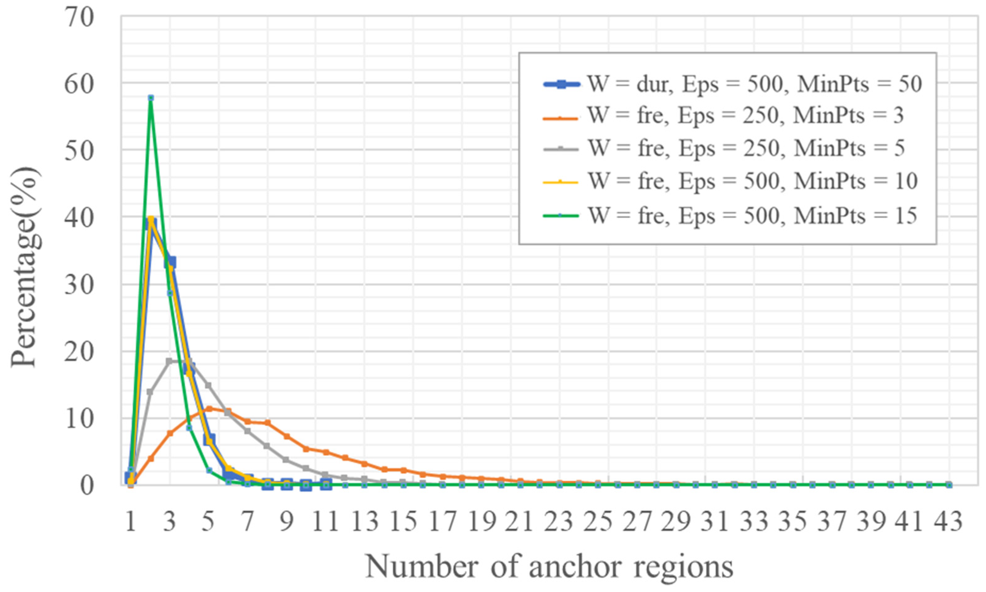
The frequency-weighted approach, particularly with parameters prioritizing sensitivity (e.g., W = fre, Eps = 250, and MinPts = 5), consistently identifies a larger number of regular locations per person (Figure A1). This aligns with the expectation that weighting by visit count amplifies the influence of short-duration, monthly visited stops (e.g., an airport), potentially causing them to be delineated as separate, smaller clusters distinct from primary anchors. This tendency is reflected in the flatter, more right-skewed distribution of anchor region numbers (Figure A2). However, further reducing MinPts to 3 (W = fre, Eps = 250, and MinPts = 3) leads to a notable increase in the maximum number of anchor regions (max = 43). This suggests that the algorithm may induce over-segmentation of the activity space, potentially by classifying more infrequent visits as distinct regular locations.
Conversely, a more restrictive parameter set (Eps = 500; MinPts = 15) produces a sharply left-skewed distribution that peaks around three anchor regions (Figure A2). Although this aligns more closely with the duration-weighted baseline (W = dur, Eps = 500, and MinPts = 50), the stricter thresholds may also omit some regular-visited locations. An intermediate configuration (Eps = 500; MinPts = 10) shows notable convergence with the duration-weighted results, suggesting a degree of methodological convergence under such settings.
Figure A1.
Number of regular locations per person under different parameterizations. In the legend, W refers to the type of the weighted DBSCAN, where ‘dur’ indicates duration-based weighting (stay time) and ‘fre’ indicates frequency-based weighting (visit count).
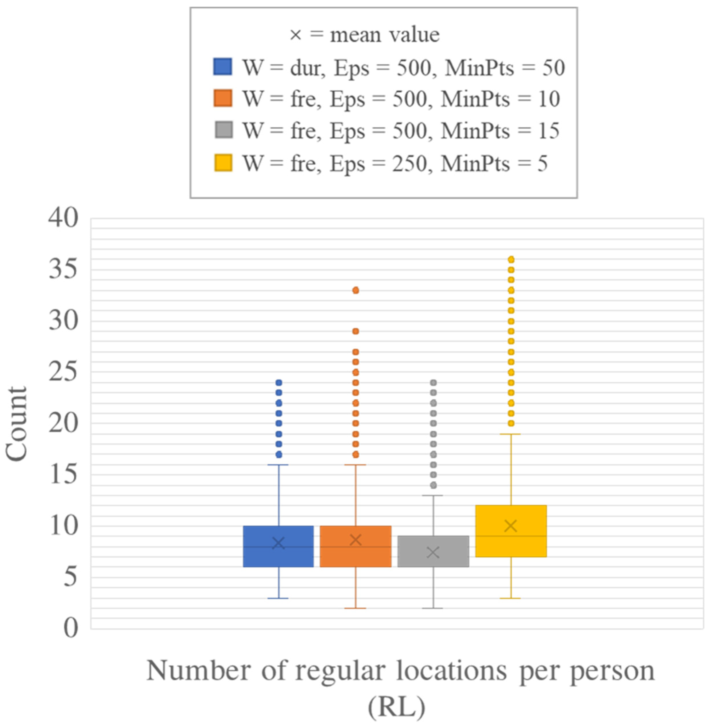
Figure A2.
Number of anchor regions per person under different parameterizations. In the legend, W refers to the type of the weighted DBSCAN, where ‘dur’ indicates duration-based weighting (stay time) and ‘fre’ indicates frequency-based weighting (visit count).
References
- Hägerstrand, T. What about people in regional science? Pap. Reg. Sci. 1970, 24, 22–145. [Google Scholar] [CrossRef] [Scilit]
- Golledge, R.G.; Stimson, R.J. Spatial cognition, cognitive mapping, and cognitive maps. In Spatial Behavior: A Geographic Perspective; The Guilford Press: New York, NY, USA, 1997; pp. 224–266. [Google Scholar]
- Xu, Y.; Belyi, A.; Bojic, I.; Ratti, C. Human mobility and socioeconomic status: Analysis of Singapore and Boston. Comput. Environ. Urban Syst. 2018, 72, 51–67. [Google Scholar] [CrossRef] [Scilit]
- Proffitt, D.G.; Bartholomew, K.; Ewing, R.; Miller, H.J. Accessibility planning in American metropolitan areas: Are we there yet? Urban Stud. 2019, 56, 167–192. [Google Scholar] [CrossRef] [Scilit]
- Zhang, S.; Yang, Y.; Zhen, F.; Lobsang, T.; Li, Z. Understanding the travel behaviors and activity patterns of the vulnerable population using smart card data: An activity space-based approach. J. Transp. Geogr. 2021, 90, 102938. [Google Scholar] [CrossRef] [Scilit]
- Schönfelder, S.; Axhausen, K.W. Activity spaces: Measures of social exclusion? Transp. Policy 2003, 10, 273–286. [Google Scholar] [CrossRef] [Scilit]
- Wong, D.W.; Shaw, S.L. Measuring segregation: An activity space approach. J. Geogr. Syst. 2011, 13, 127–145. [Google Scholar] [CrossRef] [Scilit]
- Zheng, H.; He, B.; Liu, Y.; Li, X. Deconstruction of Commuters’ Activity Space and Social Exclusion under Anchor Point Theory: A Case Study of Kunming, China. Transp. Res. Rec. 2023, 2677, 1481–1495. [Google Scholar] [CrossRef] [Scilit]
- Laatikainen, T.E.; Hasanzadeh, K.; Kyttä, M. Capturing exposure in environmental health research: Challenges and opportunities of different activity space models. Int. J. Health Geogr. 2018, 17, 29. [Google Scholar] [CrossRef] [Scilit]
- Vallée, J.; Cadot, E.; Grillo, F.; Parizot, I.; Chauvin, P. The combined effects of activity space and neighbourhood of residence on participation in preventive health-care activities: The case of cervical screening in the Paris metropolitan area (France). Health Place 2010, 16, 838–852. [Google Scholar] [CrossRef] [Scilit] [PubMed]
- Greene, M.; Hansen, A.; Hoolohan, C.; Süßbauer, E.; Domaneschi, L. Consumption and shifting temporalities of daily life in times of disruption: Undoing and reassembling household practices during the COVID-19 pandemic. Sustain. Sci. Pract. Policy 2022, 18, 215–230. [Google Scholar] [CrossRef] [Scilit]
- Kwan, M.P. From place-based to people-based exposure measures. Soc. Sci. Med. 2009, 69, 1311–1313. [Google Scholar] [CrossRef] [Scilit] [PubMed]
- Lee, J.H.; Davis, A.W.; Yoon, S.Y.; Goulias, K.G. Activity space estimation with longitudinal observations of social media data. Transportation 2016, 43, 955–977. [Google Scholar] [CrossRef] [Scilit]
- Dijst, M. Two-earner families and their action spaces: A case study of two Dutch communities. GeoJournal 1999, 48, 195–206. [Google Scholar] [CrossRef] [Scilit]
- Ta, N.; Kwan, M.P.; Lin, S.; Zhu, Q. The activity space-based segregation of migrants in suburban Shanghai. Appl. Geogr. 2021, 133, 102499. [Google Scholar] [CrossRef] [Scilit]
- Schönfelder, S.; Axhausen, K.W. Structure and innovation of human activity spaces. Arbeitsberichte Verkehrs-und Raumplanung 2004, 258, 1–40. [Google Scholar]
- Hasanzadeh, K. Exploring centricity of activity spaces: From measurement to the identification of personal and environmental factors. Travel Behav. Soc. 2019, 14, 57–65. [Google Scholar] [CrossRef] [Scilit]
- Hasanzadeh, K. Use of participatory mapping approaches for activity space studies: A brief overview of pros and cons. GeoJournal 2022, 87, 723–738. [Google Scholar] [CrossRef] [Scilit]
- Brown, L.A.; Moore, E.G. The intra-urban migration process: A perspective. Geogr. Ann. Ser. B Hum. Geogr. 1970, 52, 1–13. [Google Scholar] [CrossRef]
- Horton, F.E.; Reynolds, D.R. Effects of urban spatial structure on individual behavior. Econ. Geogr. 1971, 47, 36–48. [Google Scholar] [CrossRef] [Scilit]
- Couclelis, H.; Golledge, R.G.; Gale, N.; Tobler, W. Exploring the anchor-point hypothesis of spatial cognition. J. Environ. Psychol. 1987, 7, 99–122. [Google Scholar] [CrossRef] [Scilit]
- Kwan, M.P.; Weber, J. Individual accessibility revisited: Implications for geographical analysis in the twenty-first century. Geogr. Anal. 2003, 35, 341–353. [Google Scholar] [CrossRef] [Scilit]
- Yoo, E.H. How short is long enough? Modeling temporal aspects of human mobility behavior using mobile phone data. Ann. Am. Assoc. Geogr. 2019, 109, 1415–1432. [Google Scholar] [CrossRef] [Scilit]
- Xu, Y.; Shaw, S.L.; Zhao, Z.; Yin, L.; Lu, F.; Chen, J.; Fang, Z.; Li, Q. Another tale of two cities: Understanding human activity space using actively tracked cellphone location data. Ann. Am. Assoc. Geogr. 2016, 106, 489–502. [Google Scholar]
- Xu, Y.; Li, X.; Shaw, S.L.; Lu, F.; Yin, L.; Chen, B.Y. Effects of data preprocessing methods on addressing location uncertainty in mobile signaling data. Ann. Am. Assoc. Geogr. 2020, 111, 515–539. [Google Scholar] [CrossRef] [Scilit]
- Song, S.; Li, W.; Yu, Q.; Yang, D. Analysis of Individual’s Activity Space Based on the Cellular Signaling Data. Math. Probl. Eng. 2021, 1, 6690295. [Google Scholar] [CrossRef] [Scilit]
- Järv, O.; Ahas, R.; Witlox, F. Understanding monthly variability in human activity spaces: A twelve-month study using mobile phone call detail records. Transp. Res. Part C Emerg. Technol. 2014, 38, 122–135. [Google Scholar] [CrossRef] [Scilit]
- Yue, Y.; Lan, T.; Yeh, A.G.; Li, Q.Q. Zooming into individuals to understand the collective: A review of trajectory-based travel behaviour studies. Travel Behav. Soc. 2014, 1, 69–78. [Google Scholar] [CrossRef] [Scilit]
- Huang, Q.; Wong, D.W. Modeling and visualizing regular human mobility patterns with uncertainty: An example using Twitter data. Ann. Assoc. Am. Geogr. 2015, 105, 1179–1197. [Google Scholar] [CrossRef] [Scilit]
- Xu, Y.; Li, J.; Xue, J.; Park, S.; Li, Q. Tourism geography through the lens of time use: A computational framework using fine-grained mobile phone data. Ann. Am. Assoc. Geogr. 2021, 111, 1420–1444. [Google Scholar] [CrossRef] [Scilit]
- Chen, X.J.; Zhao, Y.; Kang, C.; Xing, X.; Dong, Q.; Liu, Y. Characterizing the temporally stable structure of community evolution in intra-urban origin-destination networks. Cities 2024, 150, 105033. [Google Scholar] [CrossRef] [Scilit]
- Liu, Y.; Hu, Y.; Wang, D.; Cheng, Y.; Yan, L.; Wei, D.; Jiao, J. Decomposing urban spatial rhythms: A big-small data fusion framework for activity pattern identification. Cities 2026, 169, 106548. [Google Scholar] [CrossRef] [Scilit]
- Wang, R.; Liu, S.; Li, W.; Sun, T. Exploring neighborhood daily activity patterns from the perspective of mobility using location-based services data: A case study of Shanghai. Appl. Geogr. 2025, 183, 103733. [Google Scholar] [CrossRef] [Scilit]
- Du, F.; Wang, J.; Mao, L.; Kang, J. Daily rhythm of urban space usage: Insights from the nexus of urban functions and human mobility. Humanit. Soc. Sci. Commun. 2024, 11, 49. [Google Scholar] [CrossRef] [Scilit]
- Liu, K.; Murayama, Y.; Ichinose, T. A multi-view of the daily urban rhythms of human mobility in the Tokyo metropolitan area. J. Transp. Geogr. 2021, 91, 102985. [Google Scholar] [CrossRef] [Scilit]
- Güller, C.; Varol, C. Unveiling the daily rhythm of urban space: Exploring the influence of built environment on spatiotemporal mobility patterns. Appl. Geogr. 2024, 170, 103366. [Google Scholar] [CrossRef] [Scilit]
- Cho, W.K.; Chung, J.H.; Kim, J. Need-based approach for modeling multiday activity participation patterns and identifying the impact of activity/travel conditions. Transp. Res. Part A Policy Pract. 2023, 172, 103665. [Google Scholar] [CrossRef] [Scilit]
- Flamm, M.; Kaufmann, V. The concept of Network of Usual Places as a tool for analysing human activity spaces. In Proceedings of the 11th World Conference on Transport Research, Berkeley, CA, USA, 24–28 June 2007; pp. 1–28. [Google Scholar]
- Ahas, R.; Silm, S.; Järv, O.; Saluveer, E.; Tiru, M. Using mobile positioning data to model locations meaningful to users of mobile phones. J. Urban Technol. 2010, 17, 3–27. [Google Scholar] [CrossRef] [Scilit]
- Susilo, Y.O.; Kitamura, R. Analysis of day-to-day variability in an individual’s action space: Exploration of 6-week Mobidrive travel diary data. Transp. Res. Rec. 2005, 1902, 124–133. [Google Scholar] [CrossRef]
- Hasan, S.; Ukkusuri, S.V. Urban activity pattern classification using topic models from online geo-location data. Transp. Res. Part C Emerg. Technol. 2014, 44, 363–381. [Google Scholar] [CrossRef] [Scilit]
- Su, R.; McBride, E.C.; Goulias, K.G. Pattern recognition of daily activity patterns using human mobility motifs and sequence analysis. Transp. Res. Part C Emerg. Technol. 2020, 120, 102796. [Google Scholar] [CrossRef] [Scilit]
- Alessandretti, L.; Aslak, U.; Lehmann, S. The scales of human mobility. Nature 2020, 587, 402–407. [Google Scholar] [CrossRef] [Scilit]
- Willberg, E.; Fink, C.; Toivonen, T. The 15-minute city for all?–Measuring individual and temporal variations in walking accessibility. J. Transp. Geogr. 2023, 106, 103521. [Google Scholar] [CrossRef] [Scilit]
- Shen, J.; Karimi, K.; Tao, Y. A framework for identifying activity groups from individual trajectories. J. Transp. Geogr. 2016, 57, 1785–1805. [Google Scholar]
- Wang, R.; Calabrese, F.; Di Lorenzo, G.; Ferreira, J., Jr.; Ratti, C. Urban activity location detection using cellular network data. Transp. Res. Part C Emerg. Technol. 2015, 52, 144–155. [Google Scholar]
- Zhao, P.; Wang, H.; Liu, Q.; Yan, X.Y.; Li, J. Unravelling the spatial directionality of urban mobility. Nat. Commun. 2024, 15, 4507. [Google Scholar] [CrossRef] [Scilit]
- Starczewski, A.; Goetzen, P.; Er, M.J. A new method for automatic determining of the DBSCAN parameters. J. Artif. Intell. Soft Comput. Res. 2020, 10. [Google Scholar] [CrossRef] [Scilit]
- Shenzhen Statistical Yearbook 2020. Available online: https://tjj.sz.gov.cn/attachment/1/1382/1382787/8386382.pdf (accessed on 31 December 2020).
- Clauset, A.; Shalizi, C.R.; Newman, M.E.J. Power-Law Distributions in Empirical Data. SIAM Rev. 2009, 51, 661–703. [Google Scholar] [CrossRef] [Scilit]
- Gonzalez, M.C.; Hidalgo, C.A.; Barabasi, A.L. Understanding individual human mobility patterns. Nature 2008, 453, 779–782. [Google Scholar] [CrossRef] [Scilit] [PubMed]
- Alessandretti, L.; Sapiezynski, P.; Sekara, V.; Lehmann, S.; Baronchelli, A. Evidence for a conserved quantity in human mobility. Nat. Hum. Behav. 2018, 2, 485–491. [Google Scholar] [CrossRef] [Scilit]
- Zhao, K.; Musolesi, M.; Hui, P.; Rao, W.; Tarkoma, S. Explaining the power-law distribution of human mobility through transportation modality decomposition. Sci. Rep. 2015, 5, 9136. [Google Scholar] [CrossRef] [Scilit]
- Zhou, X.; Zhao, Z.; Li, R.; Zhou, Y.; Palicot, J.; Zhang, H. Human mobility patterns in cellular networks. IEEE Commun. Lett. 2013, 17, 1877–1880. [Google Scholar] [CrossRef] [Scilit]
- Alessandretti, L.; Sapiezynski, P.; Lehmann, S.; Baronchelli, A. Multi-scale spatiotemporal analysis of human mobility. PLoS ONE 2017, 12, e0171686. [Google Scholar] [CrossRef] [Scilit] [PubMed]
- Kwan, M.P. The uncertain geographic context problem. Ann. Assoc. Am. Geogr. 2012, 102, 958–968. [Google Scholar] [CrossRef] [Scilit]
- Hong, J.; Shen, Q.; Zhang, L. How do built-environment factors affect travel behavior? A spatial analysis at different geographic scales. Transportation 2014, 41, 419–440. [Google Scholar] [CrossRef] [Scilit]
- Park, Y.M.; Kwan, M.P. Multi-contextual segregation and environmental justice research: Toward fine-scale spatiotemporal approaches. Int. J. Environ. Res. Public Health 2017, 14, 1205. [Google Scholar] [CrossRef] [Scilit]
- Liu, T.; Chai, Y. Daily life circle reconstruction: A scheme for sustainable development in urban China. Habitat Int. 2015, 50, 250–260. [Google Scholar] [CrossRef] [Scilit]
- Badr, H.S.; Du, H.; Marshall, M.; Dong, E.; Squire, M.M.; Gardner, L.M. Association between mobility patterns and COVID-19 transmission in the USA: A mathematical modelling study. Lancet Infect. Dis. 2020, 20, 1247–1254. [Google Scholar] [CrossRef] [Scilit]
- Wang, X.; Zhou, Z.; Xiao, F.; Xing, K.; Yang, Z.; Liu, Y.; Peng, C. Spatio-temporal analysis and prediction of cellular traffic in metropolis. IEEE Trans. Mob. Comput. 2018, 18, 2190–2202. [Google Scholar] [CrossRef] [Scilit]
- Moro, E.; Calacci, D.; Dong, X.; Pentland, A. Mobility patterns are associated with experienced income segregation in large US cities. Nat. Commun. 2021, 12, 4633. [Google Scholar] [CrossRef] [Scilit]

Disclaimer/Publisher’s Note: The statements, opinions and data contained in all publications are solely those of the individual author(s) and contributor(s) and not of MDPI and/or the editor(s). MDPI and/or the editor(s) disclaim responsibility for any injury to people or property resulting from any ideas, methods, instructions or products referred to in the content. |
© 2026 by the authors. Published by MDPI on behalf of the International Society for Photogrammetry and Remote Sensing. Licensee MDPI, Basel, Switzerland. This article is an open access article distributed under the terms and conditions of the Creative Commons Attribution (CC BY) license.