Abstract
Highway interchanges are vulnerable components of transport networks, often prone to congestion and crashes. Traditional monitoring methods like loop detectors or travel time queries often fail to capture the granular spatiotemporal distribution of bottlenecks in detail. To address this gap, this study introduces a new approach to quantify congestion and analyze bottleneck dynamics at Atlanta’s Tom Moreland Interchange, one of the nation’s most congested sites. A percent Traffic Congestion (pTC) metric was developed from the Google Maps Traffic Layer for twelve directional routes and validated against observed travel times obtained independently through the Google Maps Routes API. Traffic imagery collected every ten minutes for four months and 746 crash records were analyzed. Findings reveal distinct spatial patterns and temporal dynamics of congestion, with northbound I-85 and eastbound I-285 most affected during afternoon peaks. A quadratic model provided the best fit between pTC and travel times (R2 = 0.85), confirming pTC as a reliable congestion indicator. An LSTM model using pTC time series also accurately predicted mobility trends at the I-285 west to I-85 north bottleneck. Additionally, Seasonal-Trend decomposition using LOESS (STL) identified congestion anomalies, and their association was analyzed with crashes. The proposed methodology offers transportation agencies a cost-effective framework for monitoring, measuring, and understanding congestion in complex interchanges.
1. Introduction
Urban transportation networks worldwide face significant strain from congestion, which affects safety, mobility, and sustainable development [1,2,3,4]. Major highway interchanges are particularly prone to delays because they serve as critical nodes linking regional and interstate traffic [5]. Among these, Atlanta’s “Spaghetti Junction,” formally the Tom Moreland Interchange of I-285 and I-85, has consistently ranked high among the most congested bottlenecks in the United States [6]. With commuters, freight vehicles, and through-traffic converging, congestion at the junction significantly affects both local and long-distance travel across the southeastern U.S.
Conventional techniques—including loop detectors, traffic counts, and probe vehicle monitoring—provide useful data but are often limited in spatial and temporal resolution [2,7,8,9]. With the advent of crowd-sourced platforms and application programming interfaces (APIs) such as Google Maps Platform [10], real-time traffic data has become broadly accessible. Travel-time queries between origins and destinations enable agencies and researchers to identify congestion, quantify delays, and monitor evolving conditions with high temporal detail (e.g., [11,12]). Furthermore, color-coded traffic maps can also be transformed into congestion indices, generating time-series datasets for analysis, forecasting, and anomaly detection [8,13,14,15,16].
Existing monitoring systems, however, often lack the resolution needed to capture route-level dynamics within large interchanges. For example, a specific challenge arises when using Google Travel Time Route APIs at a four-way interchange where at least twelve queries are required, and often more to enforce route-specific paths to avoid potential detours. This may create substantial data collection costs. Moreover, congestion is highly dynamic, shifting throughout the day, and simple travel time cannot represent actual spatiotemporal variability at a finer road-segment level. More effective measurements and analytical methods are needed to capture spatial patterns and identify abnormal disruptions.
In this context, this study aims at developing a methodology to quantify and analyze congestion dynamics at Atlanta’s Spaghetti Junction. Specifically, the objectives are (1) measuring congestion across twelve routes using the percent Traffic Congestion (pTC) metric, (2) identifying temporal and spatial patterns, (3) validating pTC against observed travel times, (4) demonstrating short-term congestion prediction with pTC, and (5) linking pTC anomalies with reported crash events.
This study has significance in several aspects. First, it introduces a standardized, route-level congestion metric derived from Google Maps Traffic Layer data. Second, it validates the metric against observed travel times, demonstrating reliability. Third, it demonstrates the applicability of pTC by applying predictive modeling with machine learning for short-term forecasting. Finally, it combines congestion anomalies detected with crash data to explain extreme events. Collectively, these contributions may establish a scalable, data-driven methodology for monitoring, forecasting, and explaining congestion at complex interchanges.
2. Methods
2.1. Study Area
The Spaghetti Junction sits northeast of metro Atlanta where I-285 crosses I-85 (see Figure 1). Opened in 1987, it has grown into one of the busiest and most complicated interchanges in the U.S., carrying more than 200,000 vehicles from each direction daily based on GDOT’s 2024 annual average daily traffic (AADT) data [17]. It regularly ranks among the nation’s most congested interchanges, particularly along the I-285W to I-85N route [6]. To help ease traffic in the city center, Georgia State law bans trucks with more than six wheels—except buses and motorcoaches—from entering inside the I-285 perimeter, requiring them to use I-285 to bypass Atlanta [18]. With its tight geometry, weaving lanes, and mix of cars and heavy trucks, the interchange faces regular bottlenecks and high crash rates, especially during afternoon rush hours.
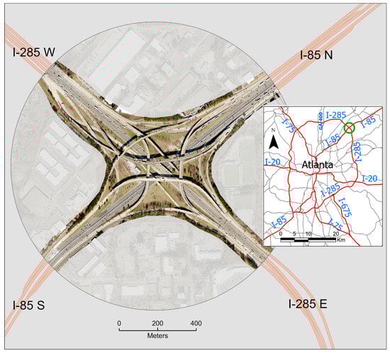
Figure 1.
Spaghetti Junction study area. Photo from 2022 Dekalb Imagery available at the following website: https://dekalbinsights-dekalbgis.opendata.arcgis.com/ (accessed on 13 November 2025). Inset road map, courtesy of the Georgia Department of Transportation. The green circle in the inset map highlights the location of Spaghetti Junction.
To address these challenges, GDOT [19] plans express lanes along the top end of I-285, including Spaghetti Junction, to relieve congestion at major junctions with I-75, GA-400, and I-85. The Atlanta Regional Freight Mobility Plan [20] also recommends an expanded collector-distributor (CD) system running parallel to I-85 North toward the county line as one of top priorities. While this expansion could bring major benefits, the impacts still need careful evaluation, according to the Plan. Altogether, these conditions make Spaghetti Junction not only a vital freight and commuter hub but also a top priority for congestion management.
2.2. Data Collection
Traffic Congestion Data. Traffic congestion data were obtained from the Google Maps JavaScript API for Static Maps [10] with the Traffic Layer enabled. The system was configured using an Apache web server with server-side JavaScript, Python 3.9, and Selenium with the Firefox driver. Screenshots (2095 rows × 2859 columns in Web Mercator projection) were captured every ten minutes from 1 April to 31 July 2025.
Figure 2 presents traffic congestion images captured at 8:00 a.m. and 5:00 p.m. on Tuesday, 22 April 2025, illustrating typical morning and afternoon traffic patterns. The stars in the figure mark the origins and destinations of the twelve study routes–EN, EW, ES, NW, NS, NE, WS, WE, WN, SE, SN, and SW; where EN represents the I-285E to I-85N route, EW the I-285E to I-285W route, and so forth.
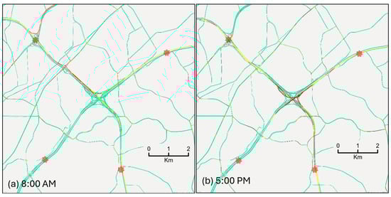
Figure 2.
Traffic congestion images on Tuesday, 22 April 2025, from Google Maps Traffic Layer. The red-star markers indicate the origins and destinations of twelve routes studied in this research.
Realtime Travel Time. Realtime travel time data were collected to validate percent congest amounts along the I-285 W to I-85 N route, focusing on afternoon and evening traffic between 2:00 P.M. and 9:00 P.M. Travel times were measured using two methods: (1) manual queries through the online Google Maps, and (2) automated collection via a Python script with the Google Maps Routes API. To ensure that measurements strictly followed the designated route rather than detours or alternate paths, a waypoint was inserted between the origin and destination. Travel time in minutes was recorded on 2 April, 8 April, 11 April, 20–25 August, 27 August, and 1 September 2025.
Route Reference Images. Because the Web Mercator projection, used in Google Maps, distorts distance significantly at mid-latitude regions, the origins and destinations of the twelve routes were identified on a map with the Universal Transverse Mercator projection, measuring approximately 4 miles long along each route. Then, the locations were marked on a Google Map image. On the Google Map with origins and destinations, each route was digitized as a single polyline. And the polyline was rasterized to create a raster route reference (RRR) image.
Crashes. Crash records were obtained from the Georgia Department of Transportation for the period between 1 April and 31 July 2025. On the twelve routes, a total of 746 crashes were reported. Among them, 211 crashes (28%) occurred on the WN route, a noticeably higher number compared to that on other routes. This study focused on the crashes along the WN route.
2.3. Congestion Metrics
Using each Google traffic image and twelve RRR images, twelve color-coded images were created by assigning 0 for the green color (no traffic), 1 for the orange color (light traffic), 2 for the red color (medium traffic), and 4 for the dark-red color (heavy traffic) [8,16]. As shown in Figure 3, each color-coded image was vectorized and then smoothed to create a final shapefile which contains multiple segments in four possible congestion categories (i.e., no traffic, light traffic, medium traffic, and heavy traffic).
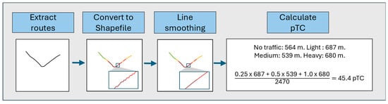
Figure 3.
Procedure of calculating pTC. An example at 16:00, 15 May, on the WN route.
From each shapefile, pTC metric was calculated using the following Equation:
where ∑ denotes the distance of light traffic segments, ∑ the distance of medium traffic segments, ∑ the distance of heavy traffic segments, and the ground distance of the route. Following previous research [8,15], weighting factors of 0.25, 0.5, and 1.0 were applied to light, medium, and heavy congestion distances, respectively. The ground distances were: EN = 5971 m, ES = 6445 m, EW = 6436 m, NE = 6095 m, NS = 6341 m, NW = 6272 m, SE = 6195 m, SN = 6388 m, SW = 6603 m, WE = 6430 m, WN = 6460 m, and WS = 6358 m. The total distance of all twelve routes was 75,994 m, and its pTC was also calculated using Equation (1). Each pTC value represents a congestion level in a route. Geographically, the congestion may be concentrated, dispersed, or in–between. For example, a pTC value of 25% could represent a case where the entire route experiences light (orange) traffic or, alternatively, where only 25% of the route is subject to heavy (dark red) congestion while the rest have no congestion.
2.4. Analytical Framework
2.4.1. Spatial and Temporal Congestion Patterns
Spatial congestion patterns were identified by mapping pTC values to highlight locations of heavy congestion bottlenecks along the twelve routes. Weekday rush hours (7:00–9:00 and 15:00–18:00) were analyzed to minimize potential statistical biases caused by free-flow or light traffic conditions and to focus specifically on commuting periods. Consequently, non-rush hours, weekends, and federal holidays—such as Memorial Day (26 May), Juneteenth National Independence Day (19 June), and Independence Day (4 July)—were excluded [21]. Because Equation (1) calculates pTC for an entire route, it does not effectively show geographical patterns on finer road segments. Therefore, another pTC at each pixel was calculated directly from color-coded image files using the following Equation (2):
where C represents a color-coded image file, i is the index of the image ranging from 1 to N, and N denotes the total number of images. For this study, N was 1105 for morning rush hours and 1615 for afternoon rush hours. Division by 4 converts weighting values of {0, 1, 2, 4} to the [0.0, 1.0] range.
Ten-minute traffic congestion data from April through July were also aggregated by hour and route to compute average congestion levels, which were then visualized in a heatmap. The weekends and holidays were excluded in this analysis, too. The heatmap was used to reveal route-specific temporal trends of congestion. Six of the most congested routes were selected, and line graphs were also created to display hourly traffic trends across each day of the week for identifying daily trends and temporal bottlenecks.
2.4.2. Validation of pTC Against Travel Time
Validation was conducted on the WN route that has been identified by ATRI [6] as one of the top ten most congested segments. Given the route’s approximate four-mile length and posted speed limit, cases with travel times under 4.4 min (i.e., free-flow conditions) were excluded to avoid potential statistical bias. Additionally, extreme outliers exceeding 60 min, such as complete standstill conditions, were excluded. Consequently, a total of 480 cases were selected for statistical modeling out of the 572 travel time observations. The goal of this validation was to examine how well the pTC metric reflects actual congestion impacts on travel time. To this end, a scatterplot was created, and linear, quadratic, and exponential models were tested as trend lines to assess the characteristics of the relationship between pTC values and observed travel times.
2.4.3. Prediction with pTC
A Long Short-Term Memory (LSTM) model [22] was applied to predict pTC values along the WN route. The prediction with LSTM was performed to evaluate forecasting effectiveness when using pTC metric in capturing temporal congestion patterns. Various LSTM models have been developed for traffic forecasting (e.g., [23,24,25,26,27,28,29]). Some recent examples include, but not limited to, a Bayesian LSTM-CNN prediction model [26], and LSTM with Sparrow Search Algorithm [29]. However, since our primary objective was to validate the predictability of the pTC metric itself, we opted for a simple LSTM model.
In this research, after multiple trials with various hyperparameters, the final LSTM model comprised a two-layer network with eight units in the first layer (configured to return sequences) and four units in the second, both regularized with L2 penalties (λ = 0.001) and followed by dropout layers with a rate of 0.4 to mitigate overfitting. The pTC input values were normalized via MinMax scaling to [0, 1] and transformed into one-step sequential samples using a sliding window of 30 time steps. The model was trained using the Adam optimizer (learning rate = 0.0005, batch size = 32). A fixed random seed (40) was applied for reproducibility. Early stopping and learning rate scheduling were employed based on validation loss to prevent overtraining and improve generalization. The dataset was split into 80% training and 20% testing, with 20% of the training portion reserved for validation. Model performance was assessed using root mean squared error (RMSE) and visual inspection of predicted versus actual values.
2.4.4. Crashes and Anomaly Detection
Using the latitude and longitude coordinates in the crash records, a point feature layer was created in geographic information systems. Then, the crashes on the twelve routes were selected manually with careful examination. A crash-prone area map was created by counting crashes using a 200 m by 200 m raster grid. The crash events were later compared with congestion anomalies to explore their potential links.
Traffic congestion anomalies were identified for the WN route using Seasonal-Trend decomposition using LOESS (STL). The STL decomposition, originally proposed by Cleveland et al. [30], splits a time series into trend, seasonal, and residual components using flexible LOESS regression. The STL decomposes a time series into additive components through a filtering procedure, allowing the analysis of dynamic time series data to estimate traffic flow and detect traffic events [31,32,33,34]. The period for STL decomposition was set to 144 because the daily cycle was represented by 144 ten-minute samples. The residuals were then standardized to obtain z-scores, and anomalies representing unexpectedly high congestion were identified using a significance level of α = 0.01 (one–tailed test, z > 2.326).
Detected anomalies were compared with actual crash records to investigate their association with traffic accidents. Crash timestamps were aggregated into ten-minute intervals, and anomalies occurring within ±30 min of a crash event were classified as crash-related anomalies, reflecting typical congestion propagation and recovery times following incidents [35,36]. The distribution of anomalies across different pTC levels was also analyzed, with the premise that severe congestion is more likely to correspond with crash occurrences.
3. Results
3.1. Congestion Patterns
When rush-hour congestion patterns were mapped (Figure 4), the northbound routes from W, S, and E showed the heaviest congestion, particularly on the curved ramp from W with more than 80% pTC. The eastbound routes from W and N also experienced heavy congestion up to 80% pTC. In contrast, the westbound and southbound routes showed relatively lighter congestion of less than 40%, with the southbound route being the lightest. Overall, the spatial pattern indicates that the north bound from the junction forms a major bottleneck section, followed by the east bound.
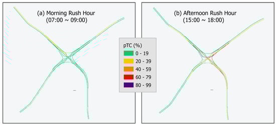
Figure 4.
Rush hour congestion patterns, (a) 07:00–09:00 and (b) 15:00–18:00.
The heatmap in Figure 5 shows that afternoon traffic is more severe than morning traffic. In the morning, medium to light traffic occurs on the NW, EW, and SW routes, which indicates congestion on the I-285 west-bound stretch. Morning traffic peaks for about one hour from 8:00 AM. In the afternoon, the WN route shows the heaviest congestion with 47.6%, followed by the WE, SN, EN, SE, and NE routes. As identified by the spatial pattern, the north stretch along I-85 is the heaviest congestion bottleneck, followed by the east stretch along I-285. The afternoon congestion peaks for about two hours from 4:00 a.m. and rapidly decreases around 7:00 p.m.
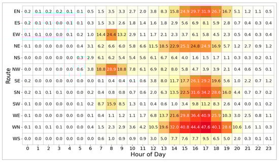
Figure 5.
Average pTC by route and hour during weekdays. In this heatmap, lighter colors represent lower congestion levels, while darker orange to red tones indicate increasingly higher congestion.
Figure 6 presents the hourly trends of pTC for the six most congested routes (EN, NW, SE, SN, WE, and WN). Congestion on Monday and Friday is generally lower than that on other weekdays. Overall, congestion patterns on Tuesday, Wednesday, and Thursday are very similar to each other. For the NW route, bimodal peaks are observed around 7:00 a.m. and 1:00 p.m. on Friday. Across all routes, Friday peak congestion occurs approximately 1–2 h earlier than peak congestion on other weekdays. During weekends, peak congestion levels are roughly one-third of the weekday peaks.
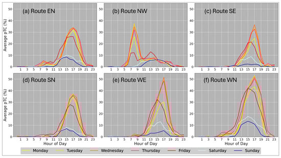
Figure 6.
Hourly traffic congestion trends by day of week. (a) EN, (b) NW, (c) SE, (d) SN, (e) WE, and (f) WN routes.
3.2. pTC vs. Travel Time
The pTC showed strong and positive relationships with travel time across all three models—linear, quadratic, and exponential—with p-values less than 0.001. As shown in Figure 7, the scatterplot and fitted curves highlight clear differences in model behavior. The quadratic model provided the best overall fit (R2 = 0.850), followed by the exponential model (R2 = 0.828), and then the linear model (R2 = 0.785). At low to moderate congestion levels, the quadratic and exponential models perform well, whereas the linear model tends to slightly overestimate travel time. At higher congestion levels, the exponential model predicts travel times that rise sharply, while the linear model tends to underestimate delays. The quadratic model provides a balance between the two models. With the quadratic model, the 25% congestion level corresponds to an average travel time of 11.04 min—about 6.64 min longer than the free-flow time of 4.4 min. As congestion increases to 50% and 75%, the expected delays grow substantially, reaching 19.79 and 39.43 min, respectively.
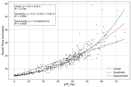
Figure 7.
Relationship between pTC and observed travel time along the WN route. Three regression models were fitted: linear (blue), quadratic (red), and exponential (green).
3.3. Congestion Prediction
In testing the effectiveness of pTC for congestion prediction, the LSTM model demonstrated effective learning and prediction of temporal traffic congestion patterns with pTC time series, achieving a test RMSE of 4.96, indicating a reasonably low prediction error. The training and validation loss curves (Figure 8a) showed stable convergence, with early stopping and learning rate scheduling to reduce overfitting. Visual comparisons between predicted and actual values across the test set (Figure 8b) revealed that the model captured general trends and fluctuations, though occasional deviations were observed during periods of rapid change. Overall, the predicted values exhibited a conservative range, tending to underestimate extremes—where the lowest forecasts remained above the actual minimums, and the highest predictions fell short of the observed peaks. A focused analysis of July 15 between 15:00 and 19:00 (Figure 8c) showed close alignment between predicted and observed congestion levels, particularly when predictions were shifted one time step backward to match the timing of actual observations. The higher pTC values during this period appear to be linked to crashes around 16:00 and 18:30, with the earlier crash lengthening congestion compared to the later one, given the higher traffic volumes during rush hour from 16:00 to 18:00.
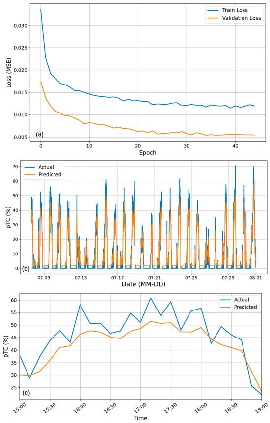
Figure 8.
LSTM prediction results. (a) Training and validation losses. (b) Actual vs. predicted values (RMSE = 4.96). (c) Actual vs. predicted values on July 15, 15:00–19:00.
3.4. Crashes and Anomalies
The spatial pattern of crash frequencies in Figure 9 reveals one major hotspot cluster (i.e., purple pixels in the figure) along the northbound stretch of I-85. Additionally, six significant hotspots (red pixels) are identified: one on the northern segment, one at the intersection center along I-85, two on the west side, and two on the east side. Among these, the merging zone on the northern stretch of I-85 emerges as the most crash-prone location, followed by clusters on the west and east segments.
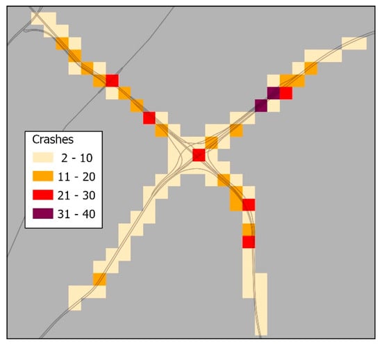
Figure 9.
Crash frequency between 1 April and 31 July 2025, aggregated to a 200 m grid.
A total of 420 anomalies were detected by the STL decomposition method. The RMSE of the STL estimation was 6.09. The RMSE value implies an approximate travel time difference of 7 min when the quadratic model in Figure 7 is applied. Figure 10a reveals weekly patterns in the trend component, where lower values appear on weekends. The average weekly range, calculated as the difference between the maximum and minimum values within each week, was about 12%, indicating that pTC typically fluctuates by about 12% over the course of a week. Figure 10b presents the seasonal component, which reveals distinct time-of-day patterns. Notably, weekends exhibit smaller fluctuations in pTC compared to weekdays, with average ranges of 34% and 47%, respectively. Combining weekly and daily fluctuations implies that congestion regularly reaches 59% on weekdays and 46% on weekends on the WN route. Figure 10c presents the residuals, calculated as the difference between the observed values and the sum of the trend and seasonal components.
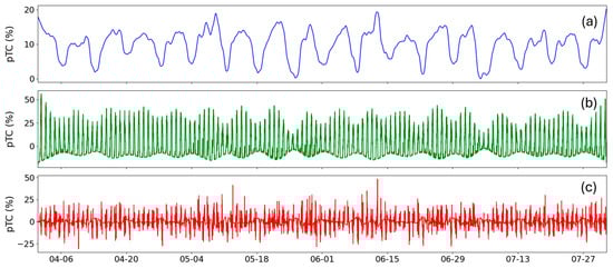
Figure 10.
STL decomposition results of pTC on the WN route. The series is decomposed into (a) trend, (b) seasonal, and (c) residual components.
Anomalies were detected with residual values where z-score values are greater than 2.326, indicating that pTC is at least 14.2 higher than the residual mean. Figure 11 shows the frequency of anomalies by weekday and time of day. The temporal distribution of anomalies revealed that they were predominantly observed during weekday afternoons. From Monday to Thursday, most anomalies occurred between 16:00 and 20:00, while on Friday, they were concentrated between 13:00 and 15:00. On Monday, anomalies were observed not only during the evening hours but also early in the afternoon, with 21 cases recorded between 12:00 and 14:00. Thursday recorded the highest total number of anomalies, with 96 cases. Particularly, 43 anomalies occurred between 19:00 and 21:00 on Thursday. During the weekend, 16 anomalies were clustered between 12:00 and 13:00 on Saturday.
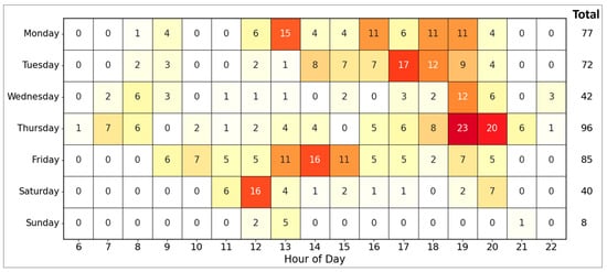
Figure 11.
Anomaly frequency by day of the week and time of day on the WN route. The numbers on the right indicate the total count for each weekday. In this heatmap, lighter colors represent lower congestion levels, while darker orange to red tones indicate increasingly higher congestion.
Figure 12 presents the overall and July 15th anomalies, further marked with crash-related anomalies. In Figure 12a, pTC values mostly remain below 40 on weekends, and anomalies occur infrequently. In contrast, during weekdays, pTC values typically exceed 40, and anomalies frequently appear around the time of daily peak congestion. While some of these anomalies are related to crashes, others are not crash-related. On July 15th (see Figure 12b), five anomalies were detected between 15:00 and 19:00. Among them two anomalies matched with the crashes occurred around 16:00 and 18:30.
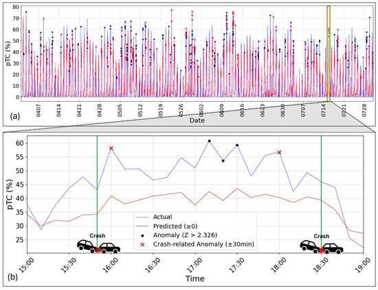
Figure 12.
Anomalies detected (black circles) and crash-related anomalies (red ‘x’ marks). (a) Anomalies for the entire study period. (b) Anomalies between 15:00 and 19:00 on 15 July.
Overall, about 29.5% of anomalies were associated with crashes, as shown in Table 1. When anomalies with pTC > 50 were analyzed, crash-related anomalies increased to 35.8%, and further to 52.5% when pTC > 60. The table shows that the percentage of crash-related anomalies rises as pTC increases up to 70 level. However, the percentage decreases when pTC > 70. This suggests that crashes are less related to unusual congestion at lower pTC values, but more strongly related at higher levels.

Table 1.
Summary of anomaly counts and crash-related anomaly ratios.
4. Discussion
The results of this study demonstrate that the pTC metric provides a robust and practical tool for measuring and analyzing congestion at a complex interchange, offering advantages over traditional volume-or speed-based indicators. By converting color-coded traffic conditions into a standardized percentage scale, pTC enables consistent comparisons across routes and time periods, even when geometric complexity or data availability limit conventional sensor-based approaches.
The validation against observed travel times confirmed that pTC reliably represents congestion impacts on travel delay, with the quadratic model yielding a strong explanatory power (R2 = 0.850). The quadratic model showed consistent curvature with a gently increasing slope, aligning with growth that was rising but still controlled. It captured the acceleration that the linear model failed to represent, while avoiding the unchecked escalation characteristic of the exponential model. Because the model’s vertex at (–7.0, 3.91) lay outside the domain of pTC [0, 100], the fitted curve remained stable, monotonic, and scientifically reasonable across the range of interest.
Beyond its temporal applications, pTC also highlights spatially critical sections where congestion mitigation efforts should be prioritized. For example, the analysis identified the northbound I-85 stretch as the most severe bottleneck, followed by the eastbound I-285 section, both of which occasionally exceeded 80% pTC during rush hours. These findings directly support the Atlanta Regional Freight Mobility Plan ([20], p.134), which prioritizes the north stretch along I-85 for the addition of an extended collector–distributor (CD) system.
The pTC metric needs to be defined carefully. As shown in Equation (1), pTC is sensitive to how the ground distance of a route is specified. A longer ground distance may reduce the pTC value, while a shorter distance focusing only on a congested section may increase it. In this study, a range of about two miles from the intersection center was used based on empirical observations. The range may be adjusted considering empirical congestion distances at different intersections. For standardization and comparison, however, we suggest using 0.5, 1, or 2 miles from an intersection center for small, moderate, and large intersections, resulting in pTC0.5, pTC1.0, and pTC2.0 metrics, respectively. In addition, pTC can be calculated separately for approaching or exiting sections of a route, such as pTC2.0E indicating 2.0 miles of exiting section to an intersection center. For example, in the case of the NS route, congestion beyond the intersection center is negligible, making pTC2.0E a more appropriate metric than using the entire route (i.e., pTC2.0) with both approaching and exiting sections.
Regarding the prediction of traffic congestion, the findings support the practical viability of LSTM-based models for short-term traffic forecasting, particularly when paired with interpretable metrics like pTC. While a simple LSTM was used to demonstrate pTC’s viability, this approach can be sensitive to noise; therefore, more advanced architectures may improve accuracy and reliability. As suggested by recent literature [25,26,27,28,29], future work could achieve higher accuracy by integrating the pTC metric with hybrid, optimized architectures or Transformer-based models, which may offer better generalization.
While the model effectively captured temporal dependencies and achieved low overall prediction error, it exhibited a tendency to overfit at multiple other trials with different sets of hyperparameters, particularly in response to short-term fluctuations and noise. This sensitivity to local variations, while beneficial for capturing fine-grained dynamics, can compromise generalization and lead to unstable predictions in less structured or anomalous traffic conditions. The use of dropout, L2 regularization, and early stopping helped mitigate overtraining to some extent, but the inherent volatility of LSTM outputs suggests that further architectural refinement may be necessary [37]. Moreover, integrating external factors—such as weather, incidents, or temporal context—may help stabilize predictions and reduce reliance on purely historical patterns [38,39,40,41].
The relationship between traffic anomalies and crash occurrences also implies several insights. Anomalies were predominantly observed during weekday afternoon peak periods, particularly between 16:00 and 20:00. This reflects typical commuting traffic patterns in metropolitan areas. However, deviations were noted around holidays such as Memorial Day and the following day, where traffic volume and congestion patterns diverged from regular weekday dynamics. These irregularities suggest the importance of accounting for holiday and special-event effects when modeling traffic anomalies, as ignoring them may lead to misclassification of unusual congestion as crash-related or non–crash-related.
In the analysis of crashes and anomalies, the crash frequency map showed the same spatial patten as the spatial congestion pattern, where higher congestion levels tied to larger crash counts. As described in the results, larger pTC levels tend to increase the percentage of crash-related anomalies. However, as shown in Table 1, the percentage decreases at pTC > 70, which is against the tendency. One explanation could be that, at extreme congestion levels, the percentage decreases, possibly because anomalies last longer than the 30 min time frame defined in this study for crash-related events. Frequently, extremely severe congestion may persist beyond 30 min resulting in underestimation of crash-related anomalies. Expanding or dynamically adjusting this temporal window based on empirical congestion recovery times could improve the robustness of the analysis. Overall, the anomality study demonstrates the utility of combining pTC time-series decomposition with crash records to identify traffic disruptions and their potential causes.
Finally, the methodology developed in this study may present challenges for users without prior experience in geographic information systems, as it involves technical processes such as server-side scripting, map projections, image-to-vector transformations, and feature summarization [42]. Future research should focus on addressing these technical barriers by developing simplified approaches for calculating pTC, including alternative sampling methods that require less specialized expertise.
5. Conclusions
This study developed and applied a new methodology for quantifying congestion at Atlanta’s Spaghetti Junction using the pTC metric derived from real-time Google Maps data. The pTC metric successfully demonstrated measuring congestion across 12 routes, examining spatial and temporal trends, validating pTC against observed travel times, implementing short-term forecasting, and detecting anomalies along with trend and seasonality. Results showed that the northbound I-85 and eastbound I-285 segments represent primary bottlenecks, with afternoon congestion generally more severe than morning congestion and Friday peaks occurring 1–2 h earlier than other weekday peaks. Validation confirmed that pTC is a reliable proxy for travel delay, with the quadratic model yielding the highest explanatory power (R2 = 0.850) among those tested. The LSTM forecasting model achieved a test RMSE of 4.96, demonstrating effectiveness of using pTC for traffic congestion prediction. The study identified 420 traffic anomalies through STL decomposition, with 29.5% linked to crashes and the proportion of crash-related anomalies increasing to 62.5% for cases exceeding 65% pTC. These findings confirm that anomalies at higher congestion levels are more likely to coincide with crashes, supporting the use of anomaly analysis as a complementary diagnostic tool. These findings suggest that pTC might help transportation agencies and urban planners not only track routine congestion trends but also pinpoint spatially sensitive zones where infrastructure improvements, operational adjustments, or targeted interventions could yield the greatest benefits.
Author Contributions
Conceptualization, Jeong Chang Seong, Jiwon Yang, Jina Jang, Chul Sue Hwang and Seung Hee Choi; validation, Jeong Chang Seong, Jina Jang, Jiwon Yang and Seung Hee Choi; formal analysis, Jeong Chang Seong, Jina Jang, Jiwon Yang and Seung Hee Choi; resources, Jeong Chang Seong and Chul Sue Hwang; data curation, Jeong Chang Seong, Jina Jang, Jiwon Yang and Brian Vann; writing—original draft preparation, Jeong Chang Seong, Jina Jang and Jiwon Yang; writing—review and editing, Jeong Chang Seong, Jina Jang and Jiwon Yang; visualization, Jeong Chang Seong, Jina Jang and Jiwon Yang; supervision, Jeong Chang Seong and Chul Sue Hwang; project administration, Jeong Chang Seong and Chul Sue Hwang; funding acquisition, Jeong Chang Seong and Chul Sue Hwang. All authors have read and agreed to the published version of the manuscript.
Funding
This research was supported by the MSIT (Ministry of Science, ICT), Korea, under the Global Research Support Program in the Digital Field program (RS-2024-00431049) supervised by the IITP (Institute for Information & Communications Technology Planning & Evaluation). The APC was also funded by Kyung Hee University.
Data Availability Statement
Sample data and Python scripts (LSTM and STL) are available at https://github.com/JiwonYang02/Spaghetti/ (accessed on 13 November 2025).
Acknowledgments
The authors thank the State Safety Data Management team members, Georgia Department of Transportation (GDOT), for providing crash data for this research. During the preparation of this manuscript, the authors used OpenAI’s ChatGPT version 5.1 for grammar checking purposes. The authors have reviewed and edited the output and take full responsibility for the content of this publication.
Conflicts of Interest
The authors declare no conflicts of interest.
Abbreviations
The following abbreviations are used in this manuscript:
| pTC | Percent Traffic Congestion |
| RRR | Raster Route Reference |
| LSTM | Long Short-Term Memory |
| STL | Seasonal-Trend decomposition using Loess |
| API | Application Programming Interface |
References
- Rodrigue, J.-P. The Geography of Transport Systems, 5th ed.; Routledge: New York, NY, USA, 2020; ISBN 9780429346323. [Google Scholar] [CrossRef]
- Wang, J.; Duan, X.; Wang, P.; Qiu, A.-G.; Chen, Z. Predicting Urban Signal-Controlled Intersection Congestion Events Using Spatio-Temporal Neural Point Process. Int. J. Digit. Earth 2024, 17, 1. [Google Scholar] [CrossRef]
- Lomax, T.; Turner, S.; Shunk, G. NCHRP Report 398: Quantifying Congestion: Volume 1—Final Report; Transportation Research Board, National Research Council: Washington, DC, USA, 1997; Available online: http://onlinepubs.trb.org/onlinepubs/nchrp/nchrp_rpt_398.pdf (accessed on 16 September 2025).
- Schrank, D.; Lomax, T. The 2005 Annual Urban Mobility Report; Texas A&M University, Texas Transportation Institute: Bryan, TX, USA, 2005. [Google Scholar]
- U.S. Federal Highway Administration. Alternative Intersections/Interchanges: Informational Report; FHWA-HRT-09-060; U.S. Department of Transportation: Washington, DC, USA, 2009.
- American Transportation Research Institute (ATRI). The Nation’s Top Truck Bottlenecks; ATRI: Washington, DC, USA, 2025. [Google Scholar]
- Chetouane, A.; Mabrouk, S.; Mosbah, M. Traffic Congestion Detection: Solutions, Open Issues and Challenges. In Distributed Computing for Emerging Smart Networks; Madria, S.K., Kolani, N., Eds.; Springer: Berlin/Heidelberg, Germany, 2021; pp. 3–22. [Google Scholar]
- Seong, J.; Kim, Y.; Goh, H.; Kim, H.; Stanescu, A. Measuring Traffic Congestion with Novel Metrics: A Case Study of Six U.S. Metropolitan Areas. ISPRS Int. J. Geoinf. 2023, 12, 130. [Google Scholar] [CrossRef]
- Kelly, T.; Gupta, J. Predicting Traffic Congestion at Urban Intersections Using Data-Driven Modeling. arXiv 2024, arXiv:2404.08838. [Google Scholar] [CrossRef]
- Google. Google Maps Platform. Available online: https://mapsplatform.google.com/ (accessed on 12 September 2025).
- Muñoz-Villamizar, A.; Solano-Charris, E.L.; AzadDisfany, M.; Reyes-Rubiano, L. Study of Urban-Traffic Congestion Based on Google Maps API: The Case of Boston. IFAC-PapersOnLine 2021, 54, 211–216. [Google Scholar] [CrossRef]
- Wei, P.; Hao, S.; Shi, Y.; Anand, A.; Wang, Y.; Chu, M.; Ning, Z. Combining Google Traffic Map with Deep Learning Model to Predict Street-Level Traffic-Related Air Pollutants in a Complex Urban Environment. Environ. Int. 2024, 191, 108992. [Google Scholar] [CrossRef]
- Zhang, S.; Yao, Y.; Hu, J.; Zhao, Y.; Li, S.; Hu, J. Deep Autoencoder Neural Networks for Short-Term Traffic Congestion Prediction of Transportation Networks. Sensors 2019, 19, 2229. [Google Scholar] [CrossRef]
- Kim, Y. Prediction of Traffic Congestion Using a Time-Series Model and Spatiotemporal Data: A Case Study of the Atlanta Downtown Connector. Georgr. Bull. 2023, 64, 7. [Google Scholar]
- Seong, J.C.; Lee, S.; Cho, Y.; Hwang, C. Beyond the Road: A Regional Perspective on Traffic Congestion in Metro Atlanta. ISPRS Int. J. Geo-Inf. 2025, 14, 61. [Google Scholar] [CrossRef]
- Ji, S.; Seong, J.; Stanescu, A.; Hwang, C.S.; Lee, Y. Spatiotemporal Traffic Database Construction with Google Real-Time Traffic Information and Spatiotemporal Congestion Pattern Analysis: A Case Study of Montgomery County, Maryland, U.S.A. J. Korean Geogr. Soc. 2021, 56, 265–276. [Google Scholar] [CrossRef]
- Georgia Department of Transportation (GDOT) GDOT Traffic Data. Available online: https://gdottrafficdata.drakewell.com/publicmultinodemap.asp (accessed on 12 September 2025).
- Georgia Office of Legislative Council. Georgia Code § 40-6-51—Restrictions on Type of Vehicle That May Travel on Certain Major Interstates and Highways Inside the Interstate 285 Perimeter. Available online: https://law.justia.com/codes/georgia/title-40/chapter-6/article-3/section-40-6-51/ (accessed on 12 September 2025).
- Georgia Department of Transportation (GDOT). I-285 Top End Express Lane Project: A Major Mobility Project—PI Number 0001758; GDOT: Atlanta, GA, USA, 2025. Available online: https://www.dot.ga.gov/systems/ProjectDocuments/Projects/0001758_I285TopEnd_ExpressLanes/FactSheets/I-285_TopEndEL_FactSheet.pdf (accessed on 16 September 2025).
- Atlanta Regional Commission (ARC). 2024 Atlanta Regional Freight Mobility Plan Report; ARC: Atlanta, GA, USA, 2024; Available online: https://cdn.atlantaregional.org/wp-content/uploads/2024-atlanta-regional-freight-mobility-plan-1.pdf (accessed on 16 September 2025).
- Zhao, P.; Hu, H. Geographical Patterns of Traffic Congestion in Growing Megacities: Big Data Analytics from Beijing. Cities 2019, 92, 164–174. [Google Scholar] [CrossRef]
- Hochreiter, S.; Schmidhuber, J. Long Short-Term Memory. Neural Comput. 1997, 9, 1735–1780. [Google Scholar] [CrossRef] [PubMed]
- Zhao, Z.; Zhang, L. LSTM Network: A Deep Learning Approach for Short-Term Traffic Flow Prediction. IET Intell. Transp. Syst. 2017, 11, 444–450. [Google Scholar] [CrossRef]
- Nguyen, H.; Bentley, C.; Kieu, L.M.; Fu, Y.; Cai, C. Deep Learning System for Travel Speed Predictions on Multiple Arterial Road Segments. Transp. Res. Rec. 2019, 2673, 145–157. [Google Scholar] [CrossRef]
- Abduljabbar, R.L.; Dia, H.; Tsai, P.W. Development and Evaluation of Bidirectional LSTM Freeway Traffic Forecasting Models Using Simulation Data. Sci. Rep. 2021, 11, 23899. [Google Scholar] [CrossRef]
- Fu, F.; Wang, D.; Sun, M.; Xie, R.; Cai, Z. Urban Traffic Flow Prediction Based on Bayesian Deep Learning Considering Optimal Aggregation Time Interval. Sustainability 2024, 16, 1818. [Google Scholar] [CrossRef]
- Waqas, M.; Abbas, S.; Farooq, U.; Khan, M.A.; Ahmad, M.; Mahmood, N. Autonomous Vehicles Congestion Model: A Transparent LSTM-Based Prediction Model Corporate with Explainable Artificial Intelligence (EAI). Egypt. Inform. J. 2024, 28, 100582. [Google Scholar] [CrossRef]
- Naheliya, B.; Redhu, P.; Kumar, K. A Hybrid Deep Learning Method for Short-Term Traffic Flow Forecasting: GSA-LSTM. Indian J. Sci. Technol. 2023, 16, 4358–4368. [Google Scholar] [CrossRef]
- Naheliya, B.; Redhu, P.; Kumar, K. Bi-Directional Long Short Term Memory Neural Network for Short-Term Traffic Speed Prediction Using Gravitational Search Algorithm. Int. J. Intell. Transp. Syst. Res. 2024, 22, 316–327. [Google Scholar] [CrossRef]
- Cleveland, R.B.; Cleveland, W.S.; McRae, J.E.; Terpenning, I. STL: A Seasonal-Trend Decomposition Procedure Based on Loess. J. Off. Stat. 1990, 6, 3–73. [Google Scholar]
- Zhu, X.; Guo, D. Urban Event Detection with Big Data of Taxi OD Trips: A Time Series Decomposition Approach. Trans. GIS 2017, 21, 560–574. [Google Scholar] [CrossRef]
- Zhao, Y.; Ma, Z.; Yang, Y.; Jiang, W.; Jiang, X. Short-Term Passenger Flow Prediction with Decomposition in Urban Railway Systems. IEEE Access 2020, 8, 107876–107886. [Google Scholar] [CrossRef]
- Chen, Y.; Wang, W.; Hua, X.; Zhao, D. Survey of Decomposition-Reconstruction-Based Hybrid Approaches for Short-Term Traffic State Forecasting. Sensors 2022, 22, 5263. [Google Scholar] [CrossRef] [PubMed]
- Zheng, Z.; Wang, Z.; Zhu, L.; Jiang, H. Determinants of the Congestion Caused by a Traffic Accident in Urban Road Networks. Accid. Anal. Prev. 2020, 136, 105327. [Google Scholar] [CrossRef] [PubMed]
- United States Department of Transportation, Federal Highway Administration. Manual on Uniform Traffic Control Devices for Streets and Highways, 11th ed.; FHWA: Washington, DC, USA, 2023. Available online: https://rosap.ntl.bts.gov/view/dot/73253 (accessed on 15 September 2025).
- Saka, A.A.; Jeihani, M.; James, P.A. Estimation of Traffic Recovery Time for Different Flow Regimes on Freeways; MD-09-SP708B4L; Morgan State University, Department of Transportation and Urban Infrastructure Studies: Baltimore, MD, USA, 2008. Available online: https://rosap.ntl.bts.gov/view/dot/17158 (accessed on 15 September 2025).
- Gomes, B.; Coelho, J.; Aidos, H. A Survey on Traffic Flow Prediction and Classification. Intell. Syst. Appl. 2023, 20, 200268. [Google Scholar] [CrossRef]
- Zhong, H.; Wang, J.; Chen, C.; Wang, J.; Li, D.; Guo, K. Weather Interaction-Aware Spatio-Temporal Attention Networks for Urban Traffic Flow Prediction. Buildings 2024, 14, 647. [Google Scholar] [CrossRef]
- Mahmassani, H.S.; Dong, J.; Kim, J.; Chen, R.B.; Park, B. Incorporating Weather Impacts in Traffic Estimation and Prediction Systems; FHWA-JPO-09-065; United States. Federal Highway Administration: Washington, DC, USA, 2009. Available online: https://rosap.ntl.bts.gov/view/dot/3990 (accessed on 15 September 2025).
- Shi, X.; Qi, H.; Shen, Y.; Wu, G.; Yin, B. A Spatial–Temporal Attention Approach for Traffic Prediction. IEEE Trans. Intell. Transp. Syst. 2021, 22, 4909–4918. [Google Scholar] [CrossRef]
- Yao, W.Q.S. From Twitter to Traffic Predictor: Next-Day Morning Traffic Prediction Using Social Media Data. Transp. Res. Part. C Emerg. Technol. 2021, 124, 102938. [Google Scholar] [CrossRef]
- Göçmen, Z.A.; Ventura, S.J. Barriers to GIS Use in Planning. J. Am. Plan. Assoc. 2010, 76, 172–183. [Google Scholar] [CrossRef]
Disclaimer/Publisher’s Note: The statements, opinions and data contained in all publications are solely those of the individual author(s) and contributor(s) and not of MDPI and/or the editor(s). MDPI and/or the editor(s) disclaim responsibility for any injury to people or property resulting from any ideas, methods, instructions or products referred to in the content. |
© 2025 by the authors. Published by MDPI on behalf of the International Society for Photogrammetry and Remote Sensing. Licensee MDPI, Basel, Switzerland. This article is an open access article distributed under the terms and conditions of the Creative Commons Attribution (CC BY) license (https://creativecommons.org/licenses/by/4.0/).