The Winds, UV Line Blanketing, Rotational Velocities and Mass Loss Rate of the Hot, Contact Binary Star TU Muscae (HD 100213)

Abstract

An empirical model of the TU Muscae binary star system has been developed by a study of 23 high resolution SWP spectrophotometric images that were obtained with the International Ultraviolet Explorer (IUE) satellite telescope including some that were downloaded from the NASA/MAST IUE Archive. The images are well distributed in Keplerian orbital phase thereby permitting a simultaneous fitting of the C IV wind-line profile by the SEI method and the light curve for the blanketed continuum (1450–1490 Å) bandpass by means of a program developed by the author. The result is a set of parameters characterizing the physical and geometric properties of the wind envelopes surrounding the stars. Surprisingly, there is no evidence for a P Cygni profile or strong, distinguishable shock front in the system, as has been found for similar investigations of EM Carinae and HD 159176. This is probably a result of the contact nature of the binary and the high-temperature environment of such a shock. That is, most of the carbon ions in the shock are more highly ionized. Based on the parameters for the SEI fit to the C IV profile, the value for the ionization fraction of C IV in the wind was calculated to be 10⁻⁴. With this value, the mass loss rate, Ṁ, calculated from two independent equations, was found to be about 10⁻⁶ solar masses per year (M_ʘ/yr). The UV line blanketing in the 1500 to 1600 Ångstrom bandpass was found to be erratically variable with orbital phase and time, indicating a variable amount of fast moving, dense clouds in the winds and/or a great amount of turbulence. The meaning of rotational velocities for the stars is problematic and depends on what point on the photospheres one is considering.

1. Introduction

A series of two previous papers has developed empirical models of the wind structure and activity for four massive, close binaries. The first of these concerned the “well-separated” pairs Y Cyg and CW Cep [1], while the remaining one studied in that paper, HD 159176, is a much tighter but not a contact system. The second paper dealt with EM Car [2]. The current contribution looks at TU Muscae (HD10023) system in a similar way. This system consists of a pair of stars with spectral types O7 V and O8 V [3] and is a true contact system (or double contact in some notation), in a similar way. A priori, one cannot tell if the contact nature of the binary will change the winds from the character known for the four binaries already studied.

A brief history for TU Mus has been summarized by Stickland et al. [4] and Terrell et al. [5], who note the importance of this very hot star, and more recently by Penny et al. [3]. The first two studies conclude with the confounding result that a high-quality UV radial velocity curve from observations with the International Ultraviolet Explorer (IUE) yields a light curve indicating an orbital inclination of 76° and a mass ratio q, which apparently disagrees significantly with the mass ratio from an adequate “blue” radial velocity curve by Anderson et al. [6], supplemented with two normal points from Terrell et al. [5] This matter has been discussed in detail by Terrell et al. [5] and they conclude that the source of the disagreement is an enigma. However, the seeming difference between the mass ratios from the two latter observational sets is not significant when realistic errors are imposed on the parameters. The most recent radial velocity analysis by Penny et al. [3] concludes that the UV radial velocity analysis yields the correct value for q.

The study by Stickland et al. [4] established precise orbital dimensions, a sin (i) = 15.41 R_⊙ and masses M₁ sin³ (i) = 15.70 M_⊙ and M₂ sin³ (i) = 9.85 M_⊙, yielding a mass ratio q = 0.627. A light curve analysis by Anderson et al. [6] yielded the orbital inclination of the system to be i = 76°. However, the study by Terrell et al. [5] determined a value of i = 77.8° and a mass ratio of 0.651, which, as mentioned above, is the same number obtained by Anderson et al. [6] within 2σ. The value for q implied from the analysis by Penny et al. [3] is 0.625.

The IUE archives hold 23 high-quality SWP images for the contact binary system TU Muscae. (The term SWP is an acronym for “Short Wavelength Primary” camera that was used to record the images). The aim of the present paper is to (1) model the winds and their interactions in this binary by means of the same IUE images used by Stickland et al. [4] for their velocity analysis, (2) study the variation in the metallicities or line blanketing in the spectra, (3) address the matter of the rotational velocities of the stars and (4) calculate the mass loss rate for the system that results from the winds.

For this binary, the Si IV and N V doublets within the SWP bandpass are too weak to provide useful information. Hence, this paper is limited to an analysis of the C IV feature near 1548 Å for the winds. This profile has been fitted with a program based on the SEI program developed by Lamers et al. [7], which was first adapted for use with binary stars by Pfeiffer et al. [8] and was referred to as BSEI. For this study, substantial improvements have been made to the BSEI program for fitting the UV line profiles. These improvements take into consideration the variable line blanketing that is observed from image to image. The results of this study have also made it possible to calculate the ionization fraction q_i for the amount of C IV in the wind and a determination of the mass loss rate for the system.

Also, an analysis of the Fe II, He II and C I spectral line features near 1640 Å was made to determine the rotational velocities of the stars. But the concept of rotational velocities for the stars in a co-rotational, over-contact system is ambiguous and such a determination is fraught with problems. As a result, there are no unique answers.

2. The Mass Ratio

The mass ratio for the TU Mus system has been a matter of contention in the literature. The situation may be summarized in this way. The visible-band photometry and spectroscopy essentially converge to a value of q = 0.651, while a UV continuum light curve, which is consistent with the UV radial velocities, leads to q = 0.625. At least formally, these two values do not overlap at a 3σ difference. There is, however, a way to understand and resolve this difference.

Choose the two photospheric temperatures given by Wilson and Rafert [9] for the system. (Their procedure cannot really determine these temperatures with high accuracy but the ratio of the temperatures is significant). These temperatures lead to theoretical flux levels in the model atmospheres of Kurucz [10] at any tabulated wavelength. For the UV continuum, the ratio of the flux levels for the two temperatures is 1.58, while the same ratio is 1.31 in the visible.

It seemed useful, therefore, to see if the UV light curve contained any information which would bear on the confused mass ratio. Bradstreet’s Program, Binary Maker 2 [11] was used by R. H. Koch [12] to calculate theoretical light curves, which preserved the parameters of Wilson and Rafert [9] but used UV limb darkening coefficients extrapolated from the calculations of van Hamme [13]. The first light curve used the value of q = 0.651 that resulted from the visible-band photometry and spectroscopy. This same program was then used to calculate a second theoretical light curve which used the UV mass ratio and preserved the contact configuration by changing to the appropriate gravitational potential. The difference between these two theoretical curves is not great, but the second one, with the mass ratio developed from the UV cross-correlation procedure used by Stickland et al. [4] was slightly to be preferred in light of the weight of the data and the associated errors. In other words, the UV continuum light curve gives no reason to prefer the visible-band mass ratio.

With the component stars in contact, the absorption and re-radiation of one star’s flux by another and the differential between the two processes is often referred to as “the reflection effect” and is very important. It displaces the light centers of the stars away from the positions of their projected mass centers toward the systemic mass center or barycenter. The effect on the cooler, fainter star is more important, because it causes that star to seem to move in a smaller orbit in the UV than in the visible. The process does logically affect both the UV continuum and the UV line centroids and accounts for the consistency of the UV spectroscopy and light curve.

The recognition of the effect is quite old and the classical understanding of it may be interpreted to mean that the visible-band mass ratio is more reliable than the UV one. However, this conclusion negates some of the force of the dictum that the UV, where most of hot star radiation is emitted, is the proper electromagnetic domain to study hot stars. Furthermore, the UV result for the mass ratio determined by Stickland et al. [4] is derived by a procedure which possesses the highest internal weight. This strongly indicates that the mass ratio given by the UV analysis is the correct one, which is in agreement with the analysis by Penny et al. [3].

3. Fitting the UV Light Curves

For HD 159176, Pachoulakis [14] showed that the UV Spectrophotometry in an IUE SWP bandpass yields a good light curve, even if the flux modulation is only that of an ellipsoidal binary light variation, and that even these modest light curves can be modeled usefully. The UV light curves for Y Cyg and CW Cep [2] had previously been found to resemble the visible-band ones if the resonance wind lines were avoided in selecting the bandpasses. Consequently, two light curves for TU Mus were extracted from the IUE spectra by integrating the observed flux over two bandpasses. The first is a continuum bandpass from 1450 to 1490 Å, and the second encompasses all of the C IV profile from 1530 to 1560 Å. A 200 Å wide bandpass between 1600 and 1800 Å was also investigated to see if an improvement in the noise in the continuum light curve could be obtained. It could not.

A study of these light curves shows that the UV radiation of TU Mus is intrinsically variable, aside from the usually binary-induced causes. Four early images lead to continuum flux levels which are consistently brighter by about 5% than the levels for all other images. Those four images were made at phases 0.158, 0.801, 0.846 and 0.887. The image at phase 0.887 was made at and earlier epoch than the other three and all four images are separated by more than 2400 days or 1700 orbital cycles from the most recent epoch. The flux difference seems to have no effect on the Doppler displacements of the photospheric lines in the study by Stickland et al. [4] and it has no known cause at present. However, it may be related to the highly variable UV line blanketing and transient emission clouds that have been discovered for the system in this paper.

The UV continuum light curve may be faced against the visible-band ones already analyzed by Anderson et al. [6] and Terrell et al. [5]. This has merit even though the IUE light curve is populated by only 19 data points (the four apparently aberrant IUE data points having been excluded). The resemblance between the three data sets is generally quite strong.

The light curve for the C IV feature has very little information in it. Although morphologically the same as the continuum one, it suffers from shot noise in the spectrum because the line is so strong. A reasonably good fit to the UV continuum light curve and u bandpass of Terrell et al. [5] has been obtained using a program developed similar to that employed by Pfeiffer and Stickland [1].

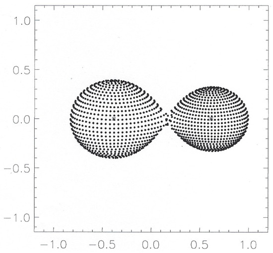
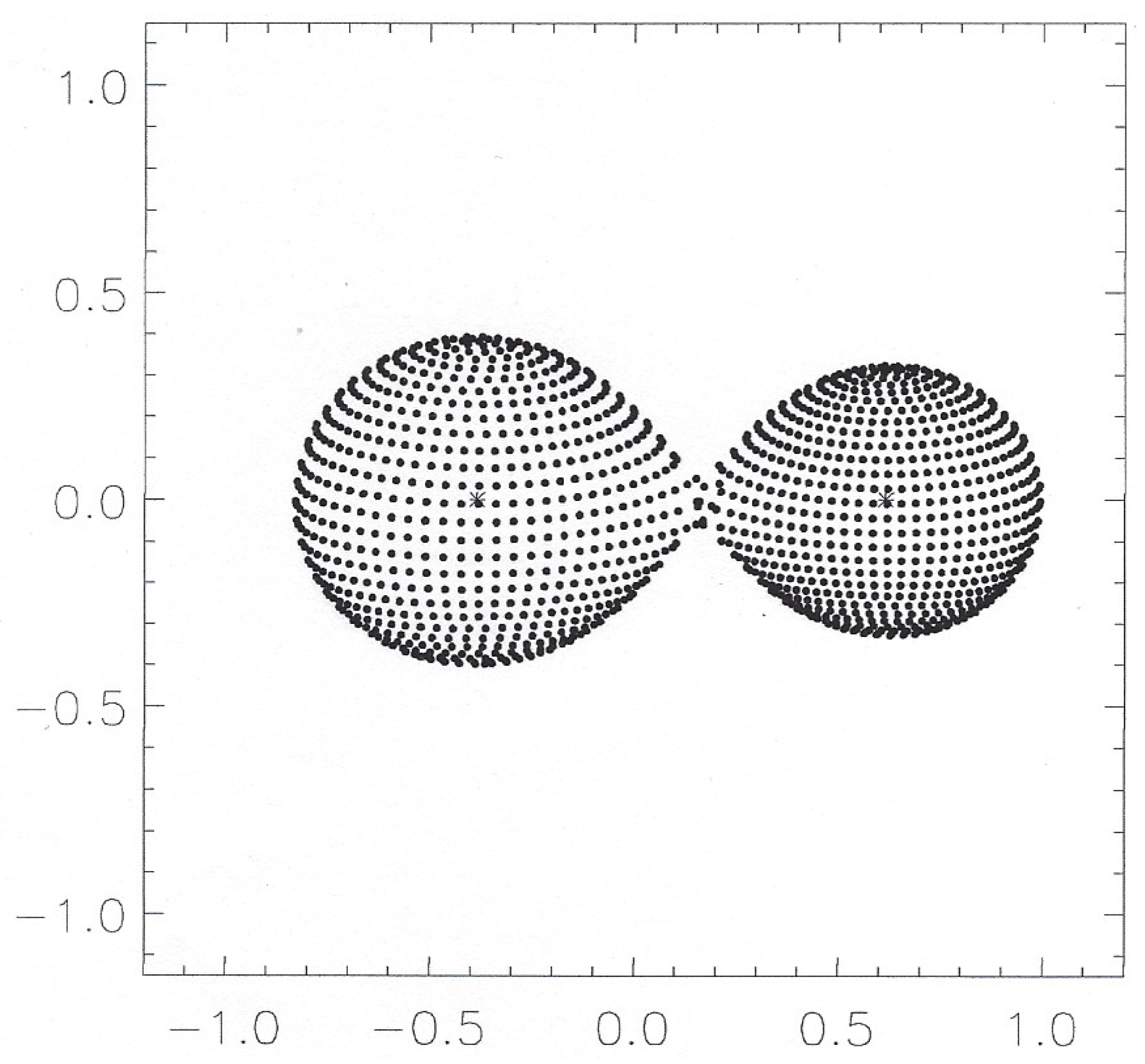
In this program, the light assigned to each star utilizes the light ratio known from the photometric solution of Terrell at al. [5]. The out-of-eclipse, integrated fiducial flux level of the system was determined to be 6.41 × 10⁻⁸ ergs/cm²/sec. This value was found by extrapolating the bandpass flux determined from the image taken at phase 0.202 to phase 0.25. This flux was then partitioned among the stars using the 3D grid of points for the stars that is shown in Figure 1.

Figure 1. The TU Mus system as represented by a grid of points seen projected onto the plane in the sky at phase 0.25. The grid was generated using the graphics available in IDL software installed on a SUN Blade 150 workstation and using a program written by the author employing techniques similar to those given in Kallrath, J. and Milone, E. F. [15]. The barycenter is located at the coordinate 0, 0 and the mass ratio of 0.625 was used. The two small stars represent the gravitational centers of the stars. The unit of distance is approximately 16 R_ʘ, based on values given in Penney et al. [3] for a₁sin (i).

The partitioning parameters are input parameters for the program and are varied to achieve a best fit. Hence, the program does not need to use the effective photospheric temperatures of the stars.

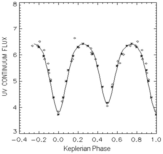
For a given set of input parameters, the light curve was generated by revolving the grid of points in orbit about the barycenter of the system and using a routine to determine which points are seen in the plane of the sky. Then all binary interaction effects are computed taking into account: (1) all ellipsoidal variations in the systemic light and (2) photosphere–photosphere eclipses. Contributions from the winds and shock were not found to be significant. The results are presented as Figure 2 below:

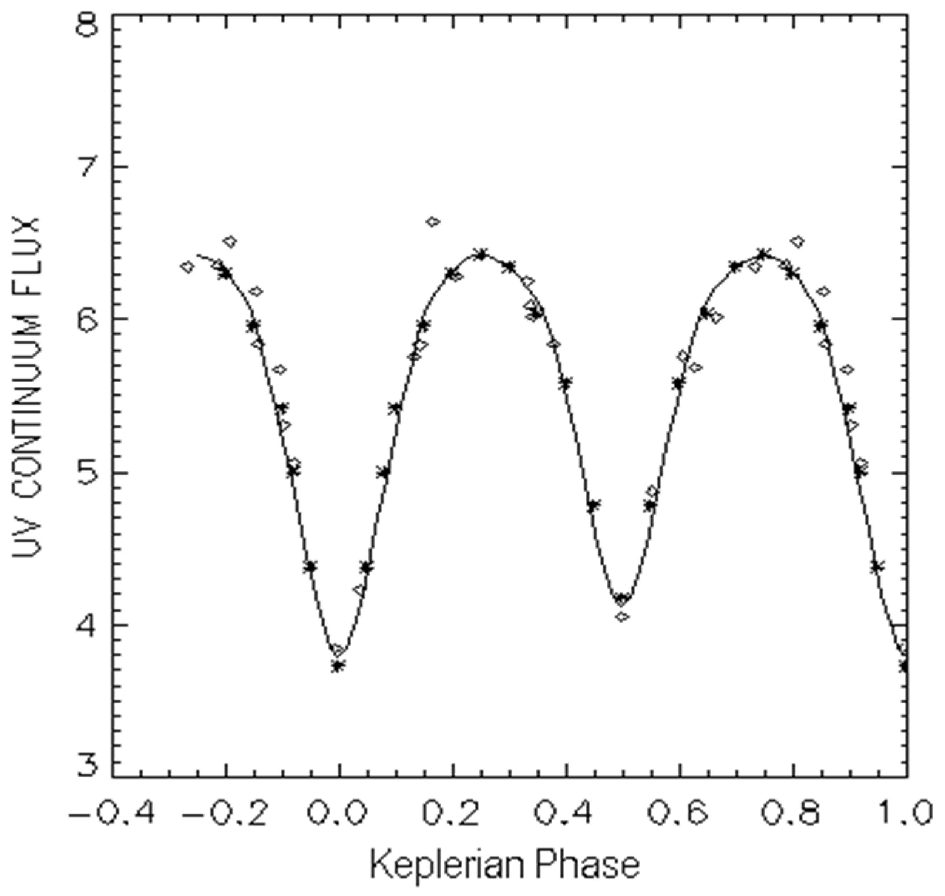
Figure 2. Displays three continuum light curves for TU Mus. The diamonds represent observations derived from the IUE-blanketed continuum (1450–1490 Å) outside the CIV line profile. The flux units are in terms of 1 × 10⁻⁸ ergs/cm²/sec. The stars are data points taken from the light curve for the u bandpass published by Terrell et al. [5] and renormalized to the IUE flux levels. The solid curve is a fit using a program developed by the author following the methodology similar to that developed by Stickland and Pfeiffer [1].

The IUE continuum flux data points, SWP numbers and phases are listed in Table A1, which is in Appendix A. Photometric orbital phases for the IUE images used in the current paper have been obtained by converting the spectroscopic phases listed in Table 1 of Penny et al. [3]. Phase 0.0 corresponds to primary conjunction, which is when the larger star is seen along the line of sight to be in front of the smaller star. There is then a minimum in the light curve. The statement “IUE blanketed continuum” means that the data points in Figure 2 are found by integrating the flux values for each wavelength data point over the specified bandpass. There are several hundred such data points that are the result of a “sliding boxing car” smoothing program of the raw data points. That bandpass does not include any part of the CIV wind-line profile. The smoothing program is one of many created by the IUE data reduction team that is available to users of IUE data.

The primary purpose of achieving such a fit is to test the algorithms so developed that, when they are integrated into the binary interaction program BSEI [1] the latter may be confidently brought to bear upon fitting the C IV wind-line profile. The binary system, as represented by these algorithms, is depicted in Figure 1.

4. The Fitting of the C IV Profile

The concern about the mass ratio is not an inconsequential one, for it determines the stellar dimensions in this contact system and thus locates the bases of the stellar winds. From the arguments presented in Section 2, it was decided to use q = 0.625, although it is not clear that this choice has to lead to the best wind geometry.

The winds can be modeled by fitting the profiles of the wind-sensitive lines. For TU Mus, the N V doublet near 1240 Å is so severely convolved with the very broad interstellar L_α line that there was no confidence in trying to isolate the stellar line. Also, the Si IV lines near 1400 Å are rather weak and give little indication of a wind. They appear to be dominated only by photospheric line absorptions. Consequently, all information about the systemic wind comes from the C IV doublet feature near 1548.2 Å. In addition, it was found that all 23 images can be used for the wind profile fitting. That is, in observed flux units, the four unusually bright images give line strengths and profiles which are indistinguishable from those of the other images. There is no current explanation why the continuum and line fluxes should be uncoupled in this way.

To begin, the SEI Program developed by Lamers et al. [7] has been modified by the author to be applicable to binary star systems and has heretofore been referred to as BSEI (Pfeiffer et al. [8]). However, the author has further improved the latter program by taking into account the line blanketing. This has been done by the addition of Gaussian profiles to fit easily recognized line profiles: the very narrow ones being interstellar absorptions and the broader ones being interstellar absorption confluences or the infamous DACs (an acronym for “Discrete Absorption clouds”) mentioned by others, such as Howarth et al. [16]. Other profiles may be actual photospheric UV line blanketing. An attempt to identify the latter was made by inspecting the spectra to see if any of these features walked in wavelength from image to image in agreement with the changing radial velocities of the stars. However, this is difficult to do, as the many lines are walking back and forth in wavelength and overlapping with one another from image to image.

For this paper, the further modified program is referred to as BSEILB. This program was then employed to fit the C IV profile for the images at photometric phases 0.053 and 0.729. Table 1 below lists the line blanketing features for the fit at phase 0.533. They are somewhat different at phase 0.229. No attempt was made to identify all the lines. They are a mixture of interstellar lines, DACs and photospheric lines. Depth is the fraction of the continuum level absorbed at the center of the line. The width is the half width in Å at half depth.

Table 1. Line blanketing features used for the C IV line profile fit at phase 0.033.

WL (Å)	Depth	Width
1533.30	0.46	1.2
1541.50	0.27	0.28
1543.70	0.15	0.60
1545.30	0.10	0.30
1549.00 CIV	0.22	0.20
1551.42 CIV	0.24	0.20
1554.25	0.14	0.22
1556.82	0.25	0.30

The original SEI fitting procedure uses normalized flux levels. But this can be misleading and may indicate a stronger P Cygni profile than what actually exists. So, in this paper, the normalized fluxes emerging from BSEILB were converted to IUE absolute fluxes. This was accomplished by using the IUE-blanketed flux levels between 1500 Å and 1600 Å, found from the dereddened IUE image to define the slope of a linear interpolation over this wavelength interval. The continuum level was set sufficiently high so that blanketing features were real and allowing for the noise in the IUE fluxes.

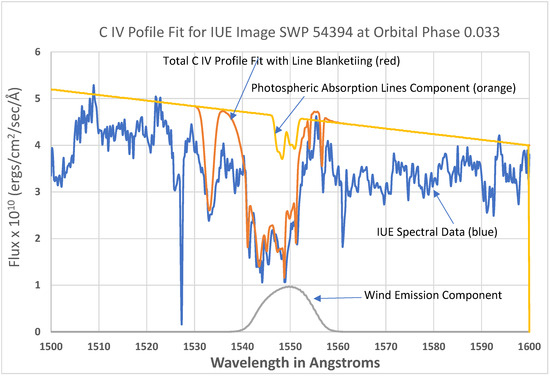
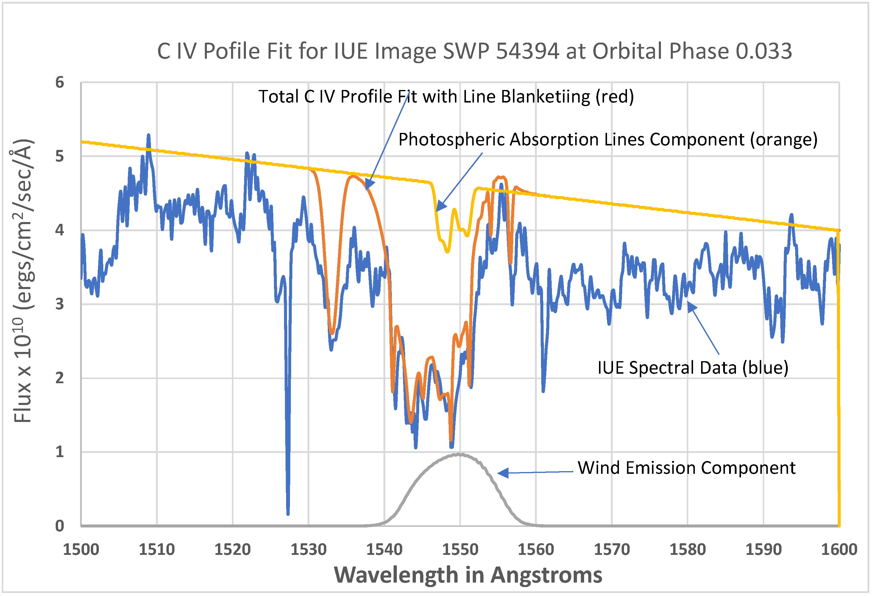
The first fit is shown in Figure 3, which clearly indicates a weak or non-existent P Cygni profile.

Figure 3. The BSEILB fit to the C IV feature at 1548 Å. The red curve is the total fit to the IUE spectral data, which are the blue curve and the yellow curve is the photospheric absorption line profiles.

The low amplitude blue feature at the bottom of Figure 3 separately displays the total wind emission, which has been modified to allow for eclipsing effects of a wind halo by the other star. The amount of such emission is critical for the best fit. The line features displayed to be hanging down from the continuum flux level are the two photospheric lines of the C IV doublet for each star. The photospheric lines have been modeled taking into account the eclipsing effects of the secondary by the primary at this phase. The proper strength of these lines, which are usually ignored in wind studies, makes it possible to achieve the fit shown.

The total fit had to match an unblanketed continuum while taking into account the shot noise both within the line profile and in the adjacent continuum between 1500 and 1600 Å. In this way, one obtains optical depths that are more accurate for the C IV ion. The two interstellar C IV lines are easily recognized and fitted. These have total widths of about 1 Å. In addition, there appear to be several other narrow lines (<2.0 Å in total width) within the bandpass, which cannot be of photospheric origin. The dictum is that a photospheric line must be rotationally broadened by about 3.3 Å in total width at the continuum as judged from the He II feature at 1640.4 Å. Such lines cannot conspire to produce narrow lines. However, several close interstellar lines can conspire to produce a broadened feature. Also, the question is which of these features are real photospheric line blanketing profiles and which are not. The answer to this was decided by comparing all the images to see which narrow features were consistently present. It was decided that if a narrow feature appeared to be at the same wavelength with the same approximate strength in three or more images, it is a real interstellar line. In some cases, an interstellar line may be obliterated by the Doppler walking of unknown photospheric lines. On the other hand, some features may be transient DACs. If the feature seemed to indicate an increasing blue Doppler shift with Keplerian phase, the probability is that the feature is a DAC.

There are two narrow lines near 1549.4 Å and 1552.0 Å that are separated by 2.6 Å, which is the nominal separation of the blue and red components of the C IV doublet. These obviously originate from an interstellar cloud that is red-shifted relative to the telescope by 0.73 Å, since the IUE images have been corrected for the motion of the satellite. Adding some of the line blanketing and interstellar absorption lines greatly facilitates obtaining the best fit to the profile. The departure of the fit from the spectrum approaching terminal velocity at wavelength 1536 Å is a result of numerous, strong line blanketing features that were not modeled. But the sharp decrease in absorption near 1541 Å is well-fitted and this was a determining factor for the input parameters.

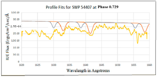
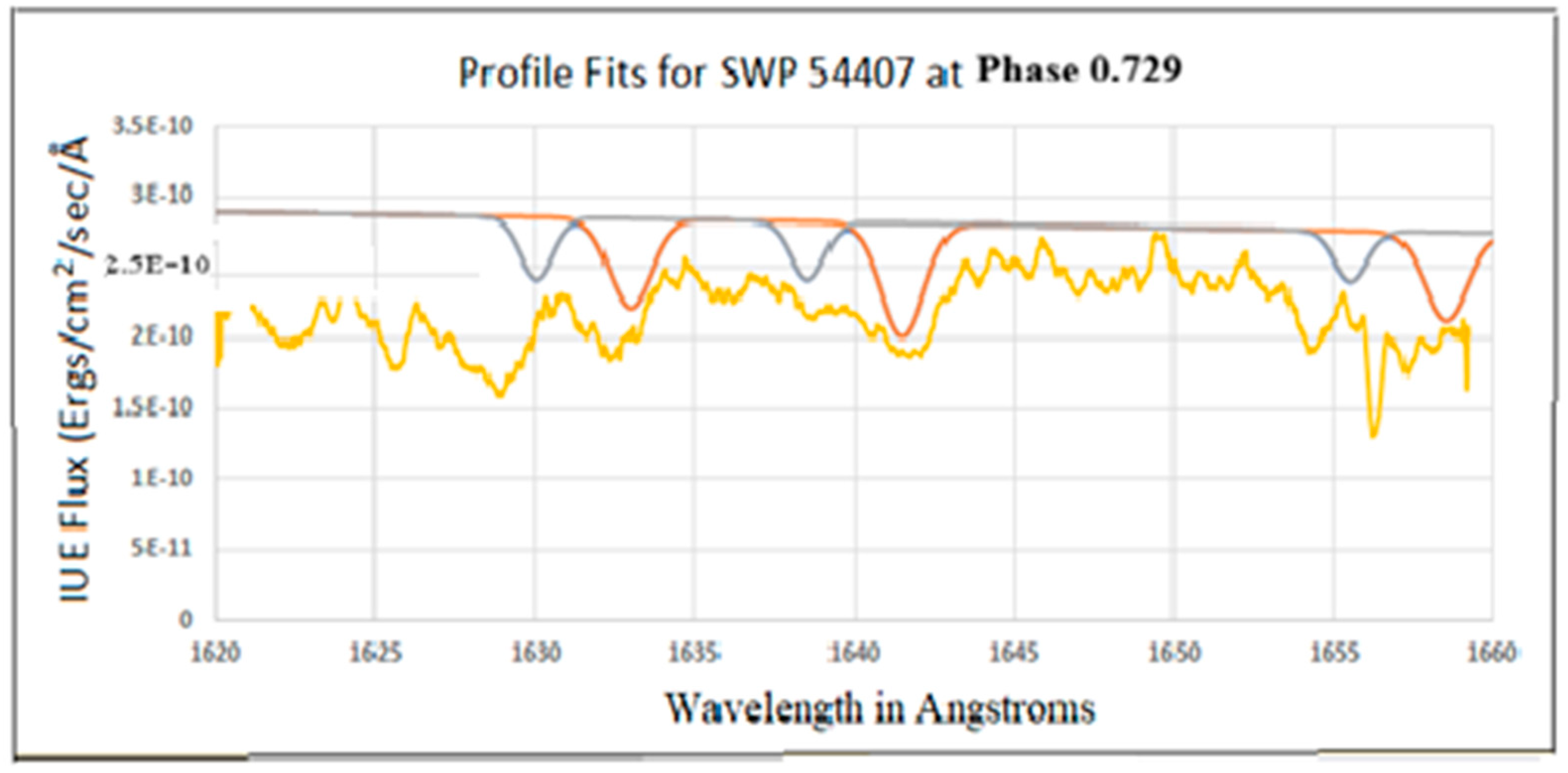
The fact that the C IV spectral feature shows no noticeable P Cygni profile at this phase is reinforced by the IUE image SWP54407, shown as Figure 4. The latter was made at orbital phase 0.729, when a possible shock and the wind envelopes are minimally eclipsed by the stars and present the best profile seen projected in the plane of the sky.

All of this may be interpreted to mean that the number density of C IV ions is low in the shock front and in the halos of the winds surrounding the stars. This probably results from the thermalization of the kinetic energy of the wind by collision that causes the ionization of the carbon ions to higher states of ionization. In fact, the work of Stevens et al. [17] indicates the temperature in a shock may exceed 10⁷ K. It may also be possible that the high intensity ultraviolet radiation from the stellar photospheres contributes to the high ionization.

Figure 4. This IUE image made at phase 0.729 also shows no evidence of a classical P Cygni profile, which should be clearly present here. The photospheric lines are purposely shown to be too strong in order to show how important they are for the best fit. An explanation of the colors is the same as for Figure 3.

Figure 4. This IUE image made at phase 0.729 also shows no evidence of a classical P Cygni profile, which should be clearly present here. The photospheric lines are purposely shown to be too strong in order to show how important they are for the best fit. An explanation of the colors is the same as for Figure 3.

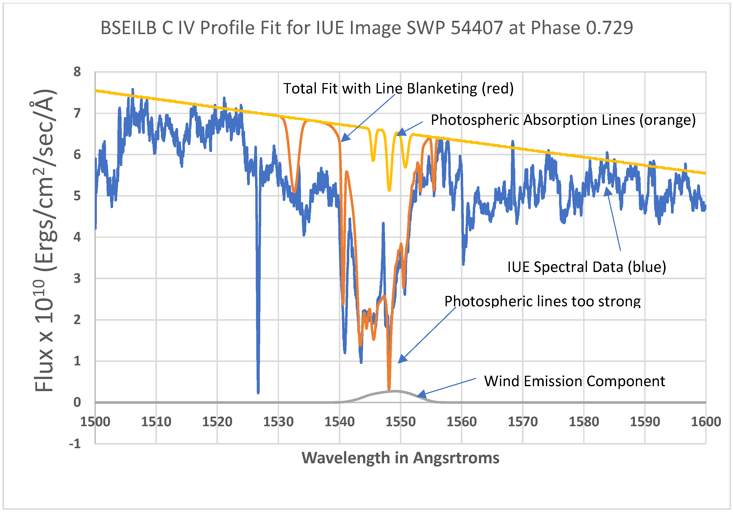
The photospheric absorption lines are relatively strong and contribute significantly to the absorption observed in the profile and indeed this doublet for both stars was modeled this way to achieve the best fit. The photospheric lines should be slightly weaker in Figure 4, but left this way to show how important they are for the best fit. The photospheric lines are weaker at phase 0.729 than at phase 0.033. (Compare the values of the SEI parameter Aphot in Table 2 and Table 3). This may be attributed to an effective increase in the density and extent of the reversing layers of the stars at the latter phase. This is the equivalent to saying that there are DACs that happened to be near the vicinity of the radial velocity-shifted wavelengths of the photospheric lines.

Table 2 presents the BSEILB parameters determined for the fit, shown in Figure 3; Table 3 shows the parameters for the fit to SWP54407. Note that DTV, and hence the terminal wind velocity, is smaller at the latter phase. Also, much more wind emission is eclipsed at phase 0.729, which is an enigma, since each star is now seen side by side in the plane of the sky, as depicted in Figure 1, rather than seen almost as one in front of the other at a conjunction.

Essentially, most of the parameter nomenclature in the tables is the one originally used by Lamars in the original FORTRAN program used for the SEI program and is as follows:

W0 is the distance from the star, in stellar radii, at which the opacity of the wind begins.

W1 is the distance from the stellar photosphere, in stellar radii, at which the terminal velocity of the wind is reached and the opacity vanishes.

WGauss is the width of the assumed Gaussian turbulent velocity distribution.

TTOTB and TTOTR are the total integrated optical depths through the wind for the blue and red wavelength components of the ion.

Alfa0 and alfa1 are parameters for determining the variation in the opacity, κρ, through the wind.

DTV is the wavelength difference between the blue component rest wavelength and the wavelength where the terminal velocity of the wind occurs.

Gamma is an exponent on the law for the variation in the opacity of the wind from the star.

AphotB and AphotR are the depths of the photospheric lines for the ion in normalized flux units.

Wphots are photospheric line widths in SEI-normalized units, not Angstroms.

Lf is the light fraction of the system contributed by each of the stars.

FWE is the fraction of the wind emission that remains after being eclipsed by the other star.

Table 2. BSEILB parameters for SWP54394 C IV at phase 0.033.

Parameter	Primary Star Wind	Secondary Star Wind
W0	0.01	0.01
W1	1.0	1.0
WGauss	0.28	0.28
TTOTB	2.50	0.50
TTOTR	1.20	0.21
Alfa0	0.05	0.01
Alfa1	7.0	7.0
DTV	12.05	12.05
Gamma	0.50	0.50
Parameter	Primary Star	Secondary Star
APhotB	0.42	0.41
AphotR	0.29	0.31
WphotB	0.05	0.05
WphotR	0.05	0.05
Lf	0.55	0.45
WFR	0.75	0.64

Table 2. BSEILB parameters for SWP54394 C IV at phase 0.033.

Parameter	Primary Star Wind	Secondary Star Wind
W0	0.01	0.01
W1	1.0	1.0
WGauss	0.28	0.28
TTOTB	2.50	0.50
TTOTR	1.20	0.21
Alfa0	0.05	0.01
Alfa1	7.0	7.0
DTV	12.05	12.05
Gamma	0.50	0.50
Parameter	Primary Star	Secondary Star
APhotB	0.42	0.41
AphotR	0.29	0.31
WphotB	0.05	0.05
WphotR	0.05	0.05
Lf	0.55	0.45
WFR	0.75	0.64

Table 3. BSEILB Parameters for SWP54407 for C IV at Phase 0.729.

Parameter	Primary Star Wind	Secondary Star Wind
W0	0.01	0.01
W1	1.0	1.0
WGauss	0.28	0.28
TTOTB	2.50	1.00
TTOTR	1.20	1.50
Alfa0	0.05	0.01
Alfa1	7.0	7.0
DTV	8.0	8.0
Gamma	0.50	0.50
Parameter	Primary Star	Secondary Star
APhotB	0.30	0.30
AphotR	0.20	0.20
WphotB	0.05	0.05
WphotR	0.05	0.05
Lf	0.55	0.45
WFR	0.27	0.25

Table 3. BSEILB Parameters for SWP54407 for C IV at Phase 0.729.

Parameter	Primary Star Wind	Secondary Star Wind
W0	0.01	0.01
W1	1.0	1.0
WGauss	0.28	0.28
TTOTB	2.50	1.00
TTOTR	1.20	1.50
Alfa0	0.05	0.01
Alfa1	7.0	7.0
DTV	8.0	8.0
Gamma	0.50	0.50
Parameter	Primary Star	Secondary Star
APhotB	0.30	0.30
AphotR	0.20	0.20
WphotB	0.05	0.05
WphotR	0.05	0.05
Lf	0.55	0.45
WFR	0.27	0.25

Surveying all the IUE images of TU Mus, one sees a variety of changes from phase to phase, some of which are phase locked and others that are transients. Particularly note the emission spike in Figure 4 near 1547 Å, which is a transient and not seen in any of the other images. Since it is blue-shifted relative to the rest wavelength of C IV, it is emission from a dense cloud moving towards the telescope, but at the side of the limb of one of the stars. It is the reverse of a DAC.

The last parameter is needed because the fluxes emanating from the system for each star are calculated separately, assuming the other star does not exist. For example, 75% of the emission from the wind of the primary star remains in Figure 3, after being eclipsed by the secondary star at the orbital phase of the system for which the fit was made. The value found for DTV (as listed in Table 2) to be 12.05 Å for both stars corresponds to a terminal velocity of 2335 km/sec. The value of DTV in Table 3 corresponds to a terminal velocity equal to 1550 km/sec. The uncertainty in DTV was just about 0.05 Å, corresponding to an uncertainty in the terminal velocity of ±10 km/sec. Somehow, the winds from both stars moving along the same line of sight toward the system may cause the difference in the terminal velocity.

Errors of the parameters are about one or two units in the last decimal pace, but such errors were difficult to determine. This is because the best fit was determined by varying all the parameters by trial and error. Some parameters were more sensitive for a best fit than others.

The determination of the BSEILB denormalization constants can be a source of error for determining the continuum level and its slope. In addition, other errors may be introduced by the assumption that the fluxes between 1500 and 1600 may be fitted by simply a linear interpolation. Nevertheless, the fits shown in Figure 3 and Figure 4 appear to be remarkably good.

5. UV Line Blanketing and Mapping Enhancements in the Density of the Winds

The spectrum of a star shows many spectral lines of various depths, or strengths, that overlap and often form confluences. The absorption of flux that these lines cause is referred to in spectroscopists’ jargon as “blanketing”. The UV line blanketing of a stellar atmosphere, z, is defined as the fraction of star’s integrated unblanketed continuum flux that is absorbed by the many metal ions in a star’s atmosphere. The absorption is commonly referred to as taking place in the reversing layer, which is the uppermost layer of a star’s photosphere.

A casual inspection of stellar spectra shows that z varies considerably over the spectrum, aside from a wind profile, such as C IV. Therefore, it is difficult to specify exactly what z is for any broad wavelength band. In addition, the question is what z should be for the observed spectrum of a binary star, since it is a composite of two stars. Furthermore, each star exudes a wind, and these winds collide and form a turbulent shock front and streams that wrap around the other star. The shock and turbulent streams in the TU Mus system probably look similar to the hydrodynamic simulations for colliding winds in OB binary stars calculated by Stevens et al. [17], as shown in Figures 12 and 15 of their paper.

All and all, the total, or integrated amount of absorbed flux, TIAF, in a spectral bandpass caused by the blanketing should remain constant, unless the wind from the companion star alters it in some way and the changing geometric and photometric changes that result from the revolution of the stars about their barycenter also induce a change. The changes in the UV line blanketing are essentially the result of an enhancement of each star’s reversing layer. This is similar to the absorption seen in the C IV profile which increases the depth of the C IV profile in addition to that caused by photospheric lines.

A priori, one would not expect that the UV line blanketing for single stars to change with time, especially short time intervals. The question remains whether the presence of a shock front, clouds or wrap-around wind streams affect the UV line blanketing. To answer this question, the value of TIAF was determined for different IUE images made at different orbital phases. The bandpass selected was 1500 to 1600 Å, excluding the wavelength interval containing the C IV feature, 1540–1552 Å. Integrated IUE flux units over a bandpass are ergs/cm²/sec. Typical shot noise in the flux of the TU Mus spectra is +/−0.07 × 10⁻¹⁰ flux units. An integration of the flux over a wide bandpass would greatly reduce this error so that uncertainty would be in the third decimal place of the values in Table 4 shown below. The changing value of TIAF rather than z is the best indication of how the wrap-around wind streams and clouds affect the UV line blanketing and allow for a mapping of this material in the system. Notice that an increase in TIAF is not always associated with an increase in z. TIUBF is the total integrated unblanketed flux, that is, the supposed unblanketed continuum that was fitted to the spectrum, as shown in Figure 3, Figure 4, Figure 5, Figure 6 and Figure 7.

The results for TIAF are also shown in Figure 5 below. The curve is somewhat erratic with sudden jumps, indicating that the wind is lumpy, consisting of various clouds that may come and go, or turbulence. The clouds may be imagined to be passing in front of the stellar photospheres of the stars as the stars revolve in orbit and the clouds may have independent motions of their own as the winds flow outwards.

Table 4. Changes in the values of TIUBF, TIAF and UV line blanketing z with orbital phase.

SWP Image	Phase	TIUBF	TIAF	z
54394	0.033	1.39 × 10−6	2.90 × 10−7	0.21
19651	0.157	2.15 × 10−6	4.32 × 10−7	0.20
54371	0.202	2.07 × 10−6	4.18 × 10−7	0.20
37906	0.326	2.05 × 10−6	3.87 × 10−7	0.19
54426	0.333	1.93 × 10−6	3.46 × 10−7	0.18
54374	0.336	1.96 × 10−6	3.87 × 10−7	0.20
37907	0.372	2.00 × 10−5	4.28 × 10−7	0.22
54378	0.492	1.36 × 10−6	3.19 × 10−7	0.24
37879	0.545	1.67 × 10−6	3.82 × 10−7	0.23
37880	0.600	1.86 × 10−6	3.68 × 10−7	0.20
54382	0.622	1.76 × 10−6	2.85 × 10−7	0.16
54353	0.658	1.90 × 10−6	3.29 × 10−7	0.17
54407	0.729	1.99 × 10−6	3.12 × 10−7	0.16
54356	0.783	1.93 × 10−6	3.05 × 10−7	0.16
19642	0.801	2.13 × 10−6	4.60 × 10−7	0.21
19643	0.846	2.35 × 10−5	3.93 × 10−7	0.17
54411	0.853	2.34 × 10−6	5.64 × 10−7	0.24
15916	0.887	1.86 × 10−6	3.89 × 10−7	0.29
54390	0.899	1.69 × 10−6	3.00 × 10−7	0.18
54360	0.916	1.73 × 10−6	4.05 × 10−7	0.23
54415	0.990	1.51 × 10−6	2.16 × 10−7	0.18

Table 4. Changes in the values of TIUBF, TIAF and UV line blanketing z with orbital phase.

SWP Image	Phase	TIUBF	TIAF	z
54394	0.033	1.39 × 10−6	2.90 × 10−7	0.21
19651	0.157	2.15 × 10−6	4.32 × 10−7	0.20
54371	0.202	2.07 × 10−6	4.18 × 10−7	0.20
37906	0.326	2.05 × 10−6	3.87 × 10−7	0.19
54426	0.333	1.93 × 10−6	3.46 × 10−7	0.18
54374	0.336	1.96 × 10−6	3.87 × 10−7	0.20
37907	0.372	2.00 × 10−5	4.28 × 10−7	0.22
54378	0.492	1.36 × 10−6	3.19 × 10−7	0.24
37879	0.545	1.67 × 10−6	3.82 × 10−7	0.23
37880	0.600	1.86 × 10−6	3.68 × 10−7	0.20
54382	0.622	1.76 × 10−6	2.85 × 10−7	0.16
54353	0.658	1.90 × 10−6	3.29 × 10−7	0.17
54407	0.729	1.99 × 10−6	3.12 × 10−7	0.16
54356	0.783	1.93 × 10−6	3.05 × 10−7	0.16
19642	0.801	2.13 × 10−6	4.60 × 10−7	0.21
19643	0.846	2.35 × 10−5	3.93 × 10−7	0.17
54411	0.853	2.34 × 10−6	5.64 × 10−7	0.24
15916	0.887	1.86 × 10−6	3.89 × 10−7	0.29
54390	0.899	1.69 × 10−6	3.00 × 10−7	0.18
54360	0.916	1.73 × 10−6	4.05 × 10−7	0.23
54415	0.990	1.51 × 10−6	2.16 × 10−7	0.18

Figure 5. The variation in the amount of TIAF (total integrated absorbed flux) or line blanketing with photometric orbital phase. The variations result from the changing density aspects of the wind as seen projected onto the photospheres of the stars. Errors are believed to be less than +/−0.01 × 10⁻⁷ flux units.

Figure 5. The variation in the amount of TIAF (total integrated absorbed flux) or line blanketing with photometric orbital phase. The variations result from the changing density aspects of the wind as seen projected onto the photospheres of the stars. Errors are believed to be less than +/−0.01 × 10⁻⁷ flux units.

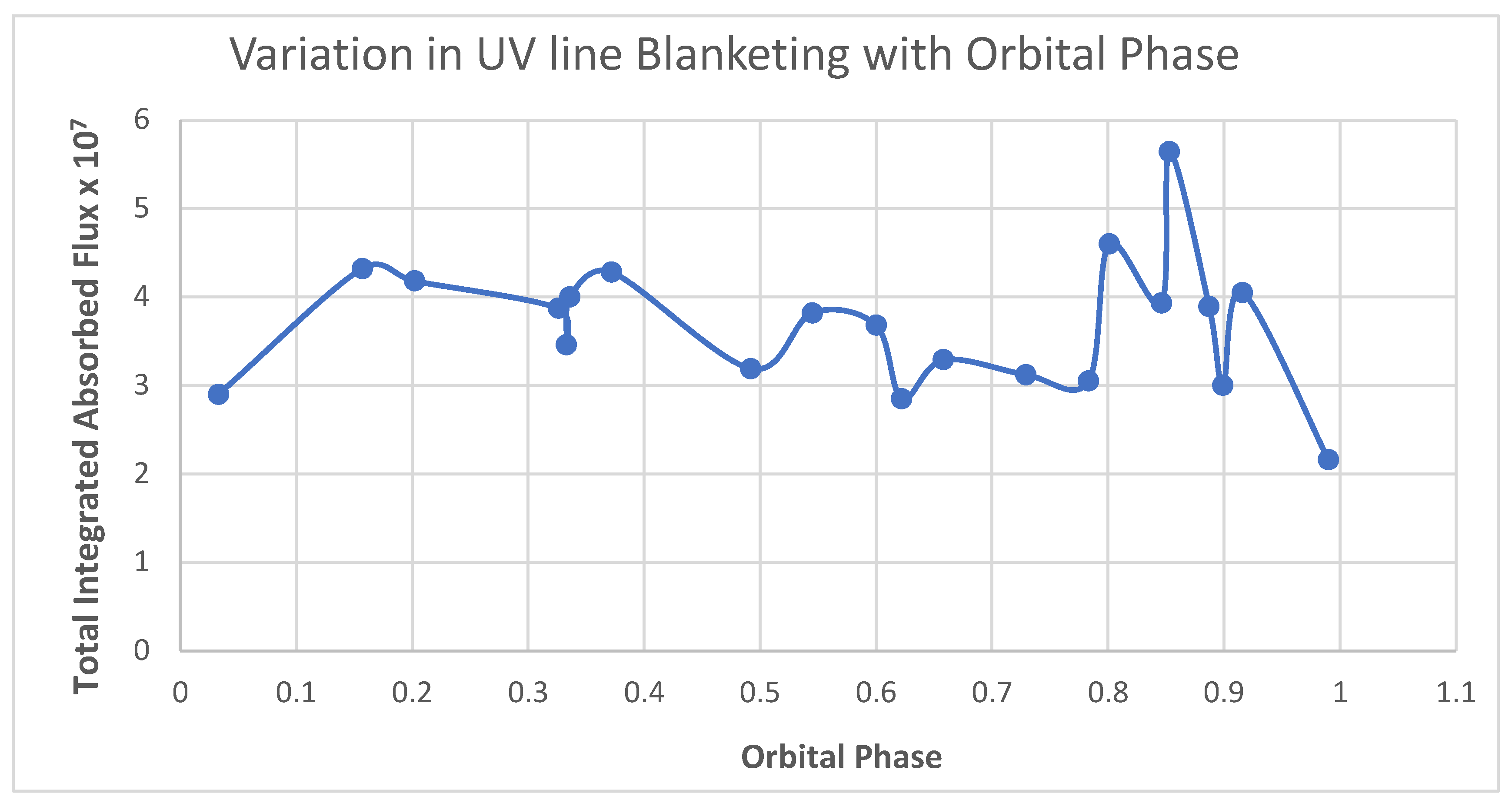
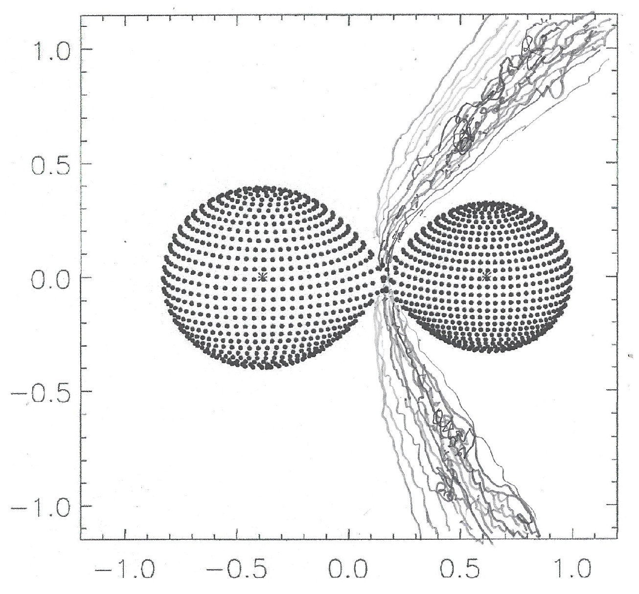
The glitch in Figure 5, between phases 0.326 and 0.336 occurred over an interval of 1993 days. The increase in UV line blanketing at phase 0.853 may be the result of a dense cloud passing in front of one of the stars at the time the image was made. It should be noted that all of this variability of the line blanketing is in phase and not time. Such variability is expected in light of the work of Stevens et al. [17]. The latter have shown that a shock would consist of various turbulent eddies that move within and along the front and that these eddies would act as clouds. A sketch of what the shock front in TU Mus might look like, imitating the results of Stevens et al. [17], has been added to Figure 1. This is depicted in Figure 6 below. It should be recalled that the wind actually occurs over a three-dimensional surface.

Figure 6. A depiction of what a hypothetical shock front might look like in the TU Mus binary star system. The asterisks mark the centers of masses of the stars.

Figure 6. A depiction of what a hypothetical shock front might look like in the TU Mus binary star system. The asterisks mark the centers of masses of the stars.

6. The Binary Stars and Wind Interactions

The program used to fit the light curve of the C IV profile is the same one simultaneously employed to fit the continuum light curves discussed in Section 3. This imposes constraints on the input parameters of the program, thereby resulting in a self-consistent method of analyzing both data sets.

At the quadrature phases, the star and wind interactions demonstrated in the IUE images are at a minimum and the light curve is at a maximum. As the stars approach conjunction, the interactions among the stars and their wind envelopes affecting the line profiles should increase. This is because the primary star is eclipsing the secondary star’s photosphere, wind envelope and a shock front between the stars. This means the depth of the wind-line changes relative to the fiducial continuum level. One might also expect that another effect will be a change in the absolute value of the metallic line blanketing z. Such changes could occur because of: (1) an ellipsoidal variation in the stellar fluxes, (2) the presence of clouds or changes in the density of the wind, and (3) photospheric eclipses. As was shown in Section 5, the presence of clouds and/or a turbulent shock front is most likely the main cause of the variation in the line blanketing, which is erratic.

At phase 0.729 (SWP54407), the dereddened continuum flux extrapolated to the center of the C IV profile is about 6.05 × 10⁻¹⁰ IUE cgs units (namely, ergs/cm²/sec). This is very nearly the maximum value for such flux, which is mainly the result of an ellipsoidal variation, since the eclipses are very shallow.

7. Rotational Velocities

The concept of stellar rotational velocities for an over-contact binary system such as TU Mus is a problematic one. During the evolution of the system, the individual rotational velocities of the two stars, as they approached one another and came into contact, were subject to tidal forces that would result in those velocities being synchronized with the orbital motions of the stars around their common barycenter. Every point on the photospheres would then revolve about the barycenter with a velocity that depends on the distance of that point from the barycenter. Hence, points on the outer limbs of the photospheres of the stars would have a higher velocity than those points closer to the barycenter. This would result in asymmetric line profiles for the photospheric spectral lines that could not be fitted with simple Gaussians. In Figure 1, it is apparent that the outer limb of the less massive star is farther from the barycenter than the outer limb of the more massive star and therefore should display a greater velocity.

With this in mind, an attempt to determine the rotational speed of the outer limb of both stars was made anyway by the simultaneous fitting of Gaussians to the Fe II feature at 1631.13 Å, the He II profile at 1640.37 Å, and the C I profile at 1657.38 Å. This was first done at phase 0.990, near primary conjunction (which is phase 0.0, when the larger star is seen in front of the smaller star) using a separate program written by the author. The result is displayed in Figure 7 below.

Figure 7. Left to right in the figure are the Gaussian profile fits for Fe II, He II and C I absorption line features in IUE SWP 54415 made at photometric orbital phase 0.990. The primary star’s lines are blue and the secondary’s are gray. The red Gaussian is the total fit. The notation E − 10 obviates using the notation 10⁻¹⁰, which takes up too much space along the vertical axis.

Figure 7. Left to right in the figure are the Gaussian profile fits for Fe II, He II and C I absorption line features in IUE SWP 54415 made at photometric orbital phase 0.990. The primary star’s lines are blue and the secondary’s are gray. The red Gaussian is the total fit. The notation E − 10 obviates using the notation 10⁻¹⁰, which takes up too much space along the vertical axis.

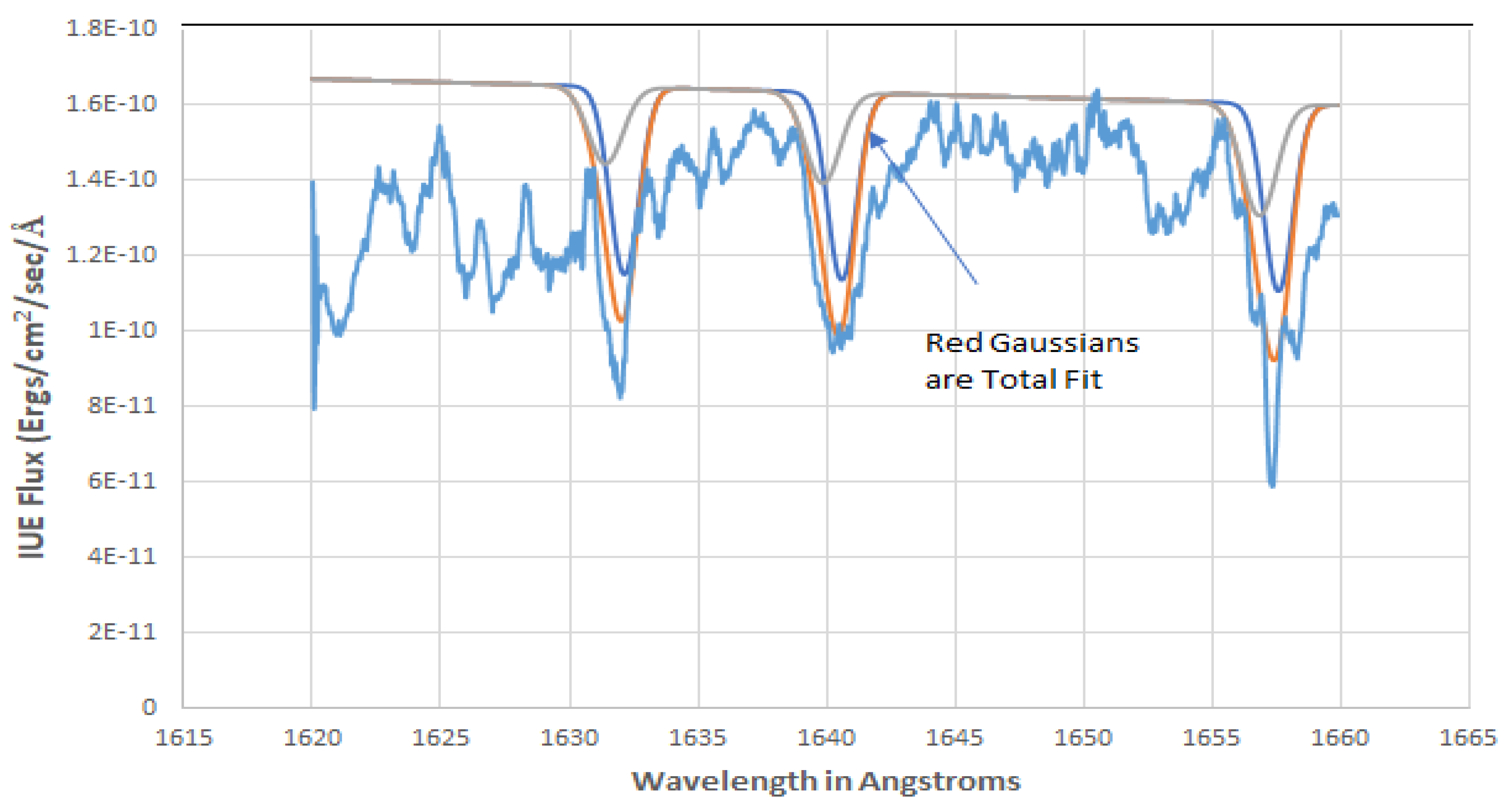
The photospheric lines of both stars making up the total profile fit (the red Gaussians) are shown separately. The lines of star 1 are the blue Gaussians, while the lines of star 2 are the gray Gaussians.

Orbital velocities of the center of mass of the stars were taken from Penney et al. [3], although these had to be changed slightly to achieve a best fit. Values for the wavelengths were taken from the online NIST ADS Catalog (Kramida, A. et al. [18]). The Fe II and C I profiles are contaminated by other lines, but the core of the He II feature looks rather pristine. There is no indication in the He II profile that He II ions are entrained in the winds in the system. The deep absorption spike below the C I feature is probably a strong C I interstellar line that is slightly blue-shifted relative to the TU Mus system.

Demanding a good fit to all three lines simultaneously puts constraints on determining the parameters for the fitting procedure, thereby allowing for a more accurate determination of the line widths. For example, wider Gaussians for the Fe II lines cannot be justified, unless one assumes that the Fe II lines are formed in a different part of the photospheres of the stars than the other lines, which is probably unlikely. In any event, Doppler rotational broadening should be the dominant factor for determining photospheric line widths. Stark broadening would only result in a wider Voight profile.

The half-widths of the Gaussian profiles at the continuum are 1.62 Å for the stars. This corresponds to a value vsin(i) = 298 +/− 5 km/sec. This value is larger by about 10 km/sec than other methods of determining the rotational speeds, such as Penny et al. [3] but is in agreement with the value obtained by Terrell et al. [5] of 290 km/sec and the value of 306 km/sec reported in the catalog of Bernacca and Perinotto [19]. However, as discussed above, the concept of individual rotational velocities for an obviously co-rotating system such as TU Mus is problematic.

The outer limb of the larger star must be co-rotating at a velocity greater than that of the center of mass of the larger star, orbital velocity, which according to Penney et al. [3] is 215 km/sec. This is in agreement with the rotational velocity for the stars to be 298 km/sec, though the limbs of the secondary should be moving at a greater velocity than the limbs of the primary.

The only way to make a precise determination of the rotational velocities is by measuring the half-widths of the profile fits at the continuum. Therefore, setting the continuum level is critical for determining the rotational velocities. Lowering the continuum would result in smaller rotation velocities and setting it higher would result in larger rotational velocities. The continuum must be properly identified taking into account the line blanketing of the spectrum and the shot noise in the flux calibration, which is about ±0.07 × 10⁻¹⁰ ergs/cm²/sec/Å in Figure 7. The line blanketing and other line confluences are strong to the short wavelength side of the Fe II feature compared with that between the He II and C I profiles. The former region of the spectrum is replete with many relatively strong, overlapping Fe II and Fe III lines. Lowering the continuum more could not be justified in light of these facts.

A fit to these same features in SWP54407 at orbital phase 0.729 has also been carried out with the same parameters. The result is shown in Figure 8, below.

Figure 8. Gaussian fits to the same features as in Figure 7, but at orbital phase 0.729, using the same input parameters and therefore the same line widths. The gold-colored curve is the IUE spectrum. The red-colored features represents the Gaussians for the primary star, whereas the blue features are the Gaussians for the secondary. The term E − 10 along the vertical axis means ×10⁻¹⁰ and obviates the need to use exponents along the ordinate numbers in the figure.

Obviously, the line profiles have a totally different appearance at this phase. For the fits shown, the photospheric line profiles for the two stars do not overlap and are seen as perfectly symmetric Gaussians. However, as mentioned above, they cannot be symmetrical profiles. Even though the individual stellar lines for these profiles are more separated, the picture is somewhat more complicated by the fact that all the other photospheric lines are overlapping and blending together. Moreover, these fits do not appear as good as those in Figure 7.

Now, the barycenter of the system is shifted from the inner LaGrangian point toward the center of the more massive star in accordance with the mass ratio. This is shown in Figure 2. In this sense, the Gaussian profiles shown above are not correct, since the profiles of the two stars should be asymmetric. At this phase, considering the limbs of the two stars, there is less of the more massive star moving towards the observer than is moving away and more of the less massive star that is moving away. This would result in asymmetric line profiles. In this sense, Figure 3 of the Hβ profile in Terrell et al. [5] is more correct but somewhat misleading, for it gives the impression that the profiles of both stars overlap and are symmetrical. Therefore, the best fit to the same profiles shown above was carried out that resulted in line widths corresponding to a rotational velocity for both stars to be vsin(i) = 516 ± 15 km/sec. This fit is displayed in Figure 9.

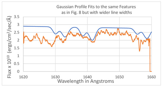
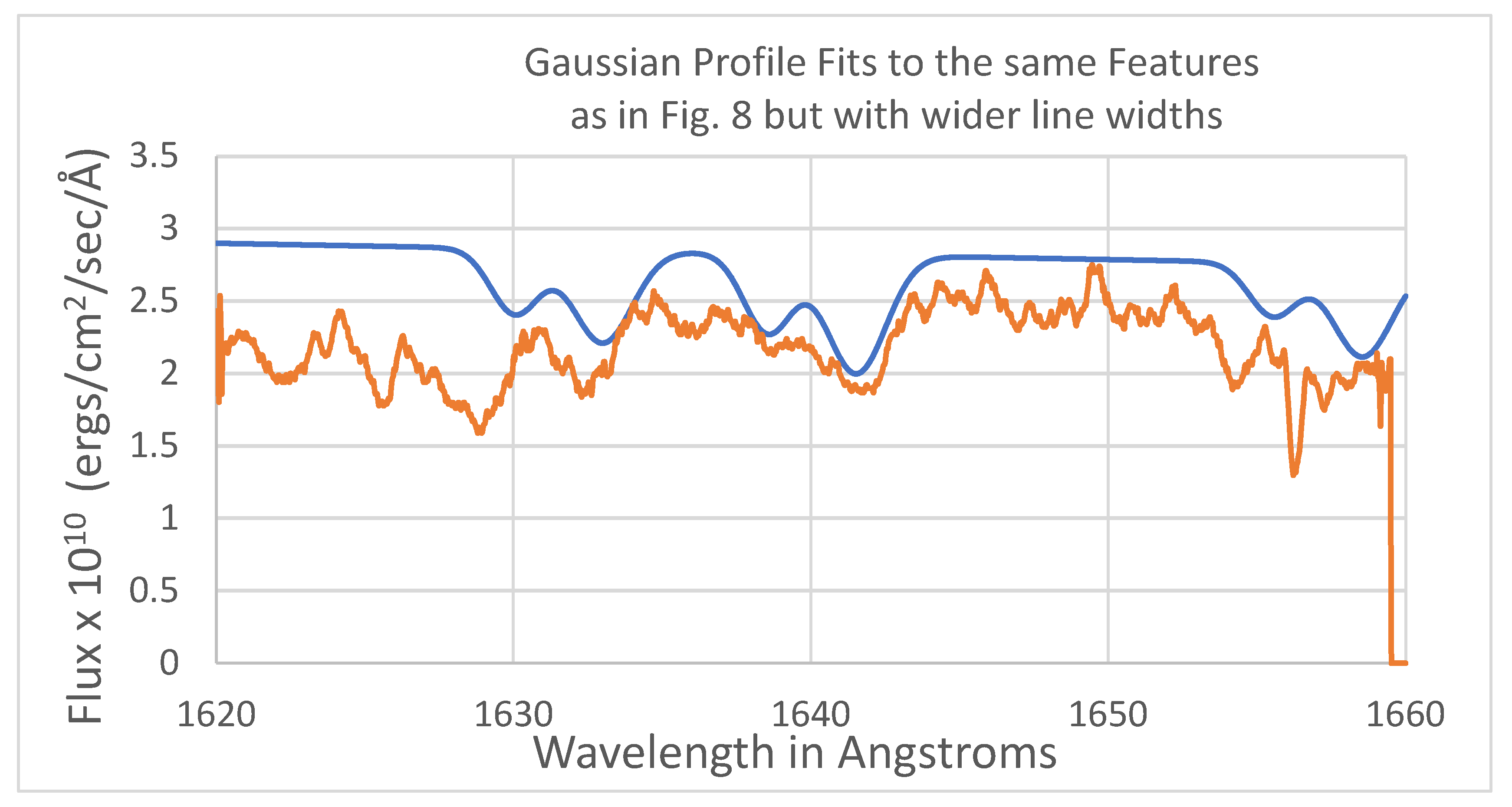
Figure 9. Profile fits to the same spectral lines as in Figure 8 but with much wider line widths to resemble overlapping symmetrical profiles. The red-colored curve is the IUE spectrum and the blue curve is the sum of the line profile fits of both stars.

In this Figure, only the total fit is shown. Indeed, the fits to all three of the line features look better and somewhat more reasonable than those in Figure 8. In addition, the profiles do resemble those in Figure 3 of Terrell et al. [5]. However, the profiles may be fitted incorrectly. The co-rotational velocity of the outer limb of the secondary, which is at a distance of 14 R_ʘ from the barycenter, is 511 km/sec in the plane of the orbit and so vsin(i) should be less. In addition, at this phase, the rotational velocity of the outer limb of the secondary should be greater than for the primary.

The result of all of this is that there is no unique rotational velocity that can be determined for the stars and that the assignment of a rotational velocity depends on what point of the photosphere of a star is being considered.

8. The Ionization Fraction, q_i, for C IV

It is possible to calculate the value of q_i if the optical depth of the wind at a distance from the photosphere is known. The optical depth τ_Δλ in bandpass Δλ is given by:

τ_Δλ = f ∫∫n(t)σ(λ)ϕ(λ)dλdt.

(1)

Here, t is the length of a path through a medium, n is the ion density, σ(λ) is the scattering cross-section and ϕ(λ) is the broadening function for a spectral line. Since we are not interested in the details of the line profile, the broadening function may be replaced by dividing the result of the integration by the Doppler-broadened width of the profile, Δλ_D. Furthermore, the scattering cross-section is constant for our bandpass, Δλ, and it will be assumed the ion density is constant along the path of length t as a first approximation. It turns out that this assumption is justified, since the variation in τ_Δλ with t is known and mainly depends on the variation in n. With the above simplifications, (1) then becomes:

τ_Δλ = f ntσ_Δλ/Δλ_D.

(2)

It follows that the number density of C IV ions in the wind, n, at distance t may then be estimated from:

n = τ_Δλ Δλ_D/(f t σ_Δλ)

(3)

Now τ_Δλ is the value of the optical depth of the wind at the distance from the star, x = r/R_⋆, which is parameterized in the SEI program by velocity w. Now, from Groenewegen and Lamars [20], Equation (5):

τ(w) = (T/I)(w/w₁)^a0{1 − (w/w₁)^1/β}^a1

(4)

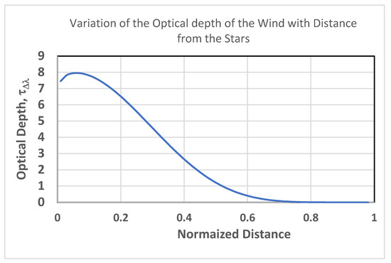
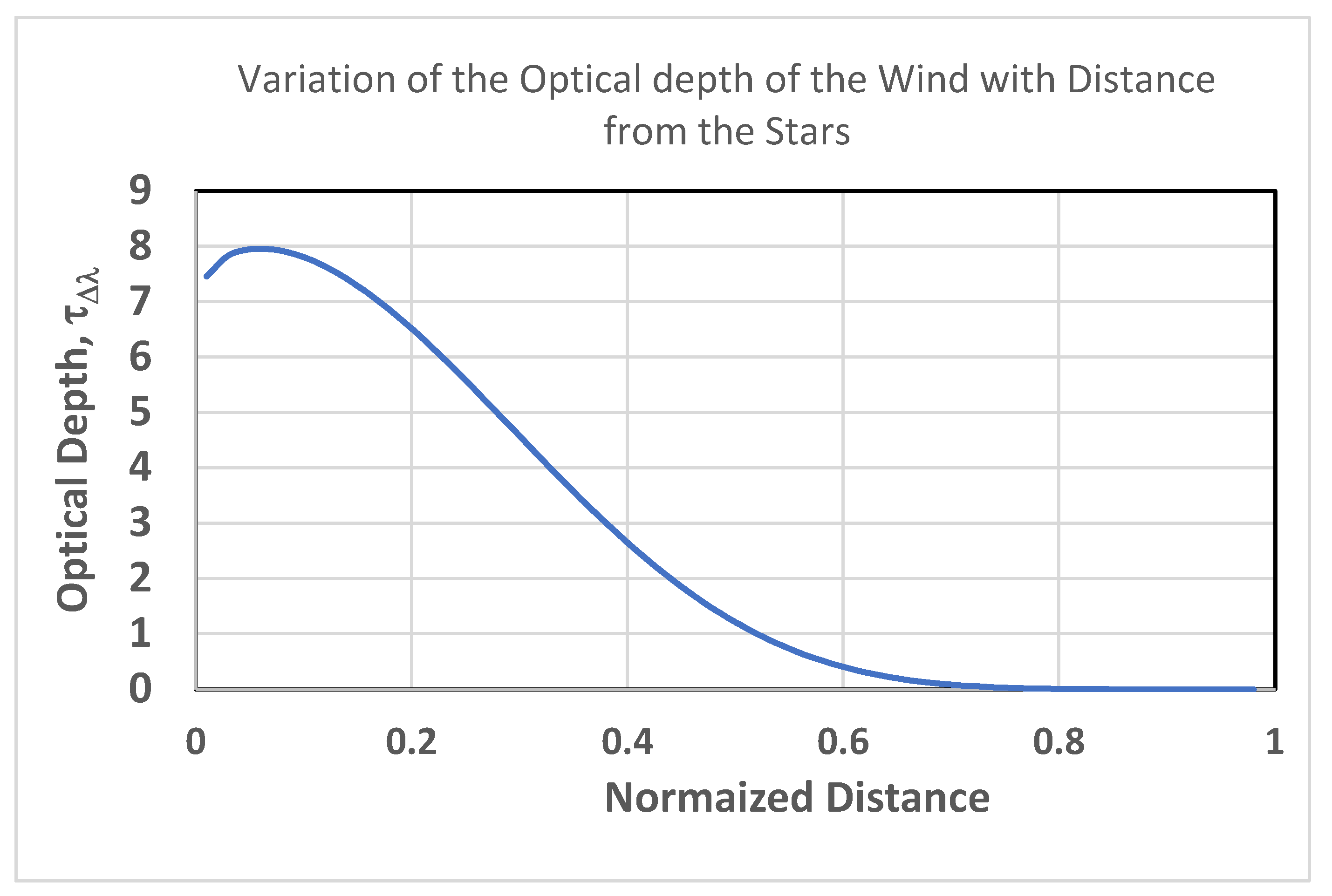
The value for (T/I) emerges from the BSEILB program and was found to be 8.897. The values of τ(w) at various values of w along the path t were then computed from (4) using the parameters in Table 2. The results are displayed as Figure 10. The total integrated optical depth along a radial path through the wind from the photosphere to where τ(w) vanishes is 2.50, which is TTOTB in Table 2.

Figure 10. Variation in the optical depth of the wind in TU Mus with distance from the photosphere. A distance 1.0 corresponds to 1 stellar radius, which is where the opacity of the wind was modeled to vanish.

The value of τ_Δλ was found to be 1.21 for w = 0.5. In addition, f is the transition probability, 0.194. The value for Δλ_D in Equation (3) is taken from the value of DTV in Table 1 and is 24 Å. The parameter t is the distance along a line of sight extending from the surface of the star to the distance where the optical depth is evaluated. In this case, t = 0.5 R_⋆ = 3.6 R_ʘ. The value σ_Δλ is the scattering cross-section, given by (πe²/m_ec)λ₀²/c, which is 2.12 × 10⁻²⁰ cm³ for the C IV profile. Hence, Equation (3) yields a value for n to be about 278 ions per cm³.

The assumption that n is constant over the path t, means the above value of n is also the value at 0.5 R_⋆. All things being equal, the ion density for the wind should follow the optical depth law, since Equation (2) shows that optical depth mainly varies as n varies. So, from Figure 10, the value of the ion density near the photosphere should be about 6.4 times greater than at x = 0.5 R_⋆. This is how one can justify removing n from the integral over t in Equation (1). The result is that n is 1780 ions/cm³ at the base of the wind.

Now, the value of the total mass density in a wind may be calculated as follows:

$${ \rho }_{wind}=(1+{\displaystyle \frac{n_{He}}{n_H}}{A}_{He}+{\displaystyle \frac{n_C}{n_H}}{A}_C+{\displaystyle \frac{n_N}{n_H}}{A}_N+{\displaystyle \frac{n_z}{n_H}}{A}_z)n_H{m}_H$$

(5)

Here A is atomic weight, $m_H$ is the mass of the hydrogen atom (and z represents all the other atoms other than helium, carbon, and nitrogen. Since the metal abundances are relatively small, they may all be represented by one term. Values for the abundance ratios relative to hydrogen were taken from Cox [21] to be 0.090 for helium, 3.63 × 10⁻⁴ for carbon and 8.80 × 10⁻³ for nitrogen. For the other metals, which are partially ionized to some unknown degree, a weighted mean value has been taken to be 20.0 for A_z and n_z/n_H = 0.0001. The exact value is not significant, since n_z/n_H is so small. The sum of all the terms in the parentheses in (4) is then 1.498 and it follows that

ρ_wind = (1.498)[n_m/(n_r/n_H)]m_H.

(6)

The number density n_m is the one measured for an atom in the wind and n_r is the number density based on the abundance of that atom relative to hydrogen.

Typical wind densities, ρ_w, for hot stars at photospheric distances of x/R_⁎ = 1 are about 10⁻¹³ g/cm³ (Lamers et al., [22], p. 251). Assuming ρ_w = 1.0 × 10⁻¹³ g/cm³ for TU Mus, Equation (6) demands that n_C be 1.45 × 10⁷ ions per cm³. Hence, the number density found for C IV, is some small fraction of all the carbon atoms in the wind. Using the value for n_CIV that was computed from (3), the fraction of C IV ions to the total number of carbon atoms, q_i, is:

q_i = 1780/1.45 × 10⁷ = 1.23 × 10⁻⁴ ≈ 10⁻⁴.

9. Mass Loss Rate

The mass loss rate may be calculated from Equation (12) in Groenewegen and Lamers [20], hereafter G&L, namely:

Ṁ = 1.189 × 10⁻¹⁸ [R_⋆v_∞²τ(w)x²w(dw/dx)][f λ₀A_Eq_i(w)]⁻¹

This was done using wind parameters from the BSEILB fit to the C IV profile. The parameters in the above equation are:

R_⋆ is the radius of the primary star in solar radii = 7.20 from Penney et al., [3]

v_∞ is the terminal velocity of the wind = 2335 km/sec.

w is the speed normalized to v_∞ and taken nominally to be 0.5 for the blue component of the doublet for the use in the above equation.

τ(w) is the optical depth at speed w: τ(w) = (T/I)(w/w₁)^a0{1 − (w/w₁)^1/β}^a1 = 1.21,

where T/I emerges from the BSEILB program to be 8.897.

The parameters a₀, a₁ and β = Gamma are given in Table 2 and Table 3.

x² = (r/R_⋆)² = (1.5)² = 2.25. Here, r is radial distance from the stellar center along the line of sight.

dw/dx = (1 − w₀)β(1− 1/x) ^(β−1)(1/x²) = 1.21. See Appendix A.

Beta is the same as Gamma in Table 2 and Table 3 above.

f is the transition probability = 0.194. (Taken from G&L, Table III)

λ₀ in Å = 1548.19

A_E is the abundance relative to H (taken from G&L, Table III): 3.2 × 10⁻⁴

q_i(w) = n_i/n_E is the ionization fraction of ion i of element E. Taken to be 10⁻⁴ based on the low density of C IV ions in the wind found from the BSEILB fitting to the C IV profile and the calculation in Section 7.

The calculation of Ṁ from the above equation is a long, tedious and intense one that, when done manually, can lead to many errors. So, the actual numerical calculations were done using a computer program. The details are presented in the Appendix B. The result is:

Ṁ = 2.51 × 10⁻⁶ M_ʘ/yr.

The uncertainty here is difficult to determine because of the uncertainties of the numerous parameters that go into the calculation. One of the reasons for this rather large value for Ṁ may be the small value assumed for q_i. But this was done considering the fact that the fit to the C IV profile indicates a low density of C IV in the wind.

Another estimate of the mass loss rate was calculated using Equation (12) from Vink, J. S., et al. [23], which is presented there as a sequence of logarithmic summations.

$$\begin{array}{cc}\hfill \mathrm{Log}\mathrm{Ṁ}& =-6.697+2.194log(\mathrm{Ls}/{10}^5)-1.313log(\mathrm{Ms}/30.0)-1.226log(\mathrm{Vr}/2.0) +\hfill \\ & +0.933log({\mathrm{T}}_{\mathrm{eff}}/40000.0)-10.92log({\mathrm{T}}_{\mathrm{eff}}/40000.0{)}^2\hfill \\ \hfill \mathrm{Log}\mathrm{Ṁ}& =-6.653+0.3239-0.1102-0.03159+0.7395\hfill \end{array}$$

Adding this sequence results in Log Ṁ = −5.731, and hence,

Ṁ = 1.86 × 10⁻⁶ M_ʘ/yr

In the above statements:

Ls is the Luminosity of the primary star, taken to be 10^5.02 L_ʘ, as given in Penny et al., [3].

Ms is the mass of the primary star taken to be 17 M_ʘ, as given in Penny et al. [3].

Vr = v_∞/v_esc = 2335/949 = 2.46, where v_esc is for a distance of R_⋆ = 7.2 R_ʘ.

T_eff of the primary taken as 37,000 K as listed in Penny et al. [3].

The above value of Ṁ is in remarkable agreement with that calculated from Equation (12) of G&L. It is also interesting that the Vink et al. equation does not include a term for the ionization fraction, q_i, and is based on statistics for hot, single stars. Because of the latter fact, it may not be applicable to contact binary star systems. The results from G&L may be more correct, since they are calculated using specific parameters for the system coming from the BSEILB fitting of the C IV profile, though the difference is not significant.

Mass Loss rates, Ṁq_i, for similar stars are listed in Table VII of G&L with values ranging from 5.01 × 10⁻⁹ to 3.98 × 10⁻¹⁰. The value of the mass loss rate for EM Car was found to be Ṁq_i = 2.7 × 10⁻⁹ by Pfeiffer and Stickland [1], but none of these values specify a value for the ionization fraction. Therefore, it is difficult to compare these results with the values found in this paper using the G&L or Vink equations. However, mass loss rates between 10⁻⁷ and 10⁻⁶ for OB binary stars are not uncommon (Stevens et al., [17]).

10. Discussion of Results

The best fits to the IUE data indicate that both stars have relatively shallow wind envelopes with densities that decrease rapidly with distance from the stars. The profile fit at phase 0.533 is very different than the one at phase 0.229 indicating a dramatic change in the geometry and density of the wind. The parameter W1 = 1 in Table 2 and Table 3 means all the absorption of the photospheric flux by the wind effectively takes place within one stellar radius from the photospheres. The fits were very sensitive to this parameter. A value of W1 = 1.5 doubled the wind emission and resulted in a P Cygni profile, which does not exist. It also extended the absorption profile to shorter wavelengths than what is seen.

The terminal velocity of the wind at orbital phase 0.033 occurs at 12.05 Å from the rest wavelength of the blue component of the C IV doublet. This translates to a terminal velocity of the wind to be 2335 km/sec, whereas the terminal velocity at phase 0.729 was 0.67 of that value. It is not clear why there is a difference, but it must be related to the difference in aspect of the wind as seen at these phases.

There is also a notable difference in the strength of the photospheric absorption lines that is also related to variable clouds in the winds or wrap-around wind streams that effectively change the reversing layers of the stars.

The W_Gauss parameter indicates some amount of turbulence in the wind flow, especially near the contact point of the stars. Including a larger amount of turbulence in the wind flow was found to produce a fit that was not as good. In effect, it causes the sharp decrease seen in the absorption near terminal velocity to be pushed to shorter wavelengths.

A geometrically separate shock between the stars cannot be detected in the spectrum, as was detected in EM Car (Pfeiffer et al. [1]). This is probably the result of the over-contact nature of the stars in TU Mus. The entire region of the common wind envelope between the stars is like a shock front and is very lumpy including various clouds and an emission cloud seen at phase 0.229 that is not seen in any other image. A study of the changing UV line blanketing of the system as revealed in Figure 5 is further testimony of this.

The apparent dearth of C IV in the winds must be a result of the high degree of ionization of C ions. The ionization potential of C IV to C V is 64.5 ev. From kinetic theory, the mean kinetic energy of all particles in the wind would have this value for T = 500,000 K. The average speed of the wind at a distance of 0.5 stellar radius is about 1000 km/sec, since the terminal velocity of the wind at one stellar radius has been determined to be about 2300 km/sec. Assuming the wind mainly consists of H and He ions in the ratio of 7 to 3, and if their speed is thermalized due to turbulence in the wind, then T = mv²/3k = 765,000 K.

But the temperature in the wind does not need to be this high to ionize C IV to higher states of ionization. Even at T = 39,000 K, the Maxwell–Boltzmann kinetic energy distribution function indicates that, in the high energy tail of the distribution, there are some particles with this energy. One must also consider the very short wavelength radiation from the photospheres of the stars that bathes the winds. For a surface temperature of 38,700 K for the primary, taken from Penney et al. [3], Wien’s Law gives a value of 749 Å for λ_max. Also, all photons carrying 64.5 ev or more correspond to a wavelength of 64.1 Å, which is just inside the X-ray region of the EM spectrum. From the black body curve for 38,700 K, there should be copious amounts of photons flowing into the winds to result in a high amount of ionization for most ions and, therefore, a high electron density.

So, it is a wonder that there is any C IV present to produce the absorption seen in the C IV profile. However, the Saha ionization equation does indicate that a high electron density environment in the winds could result in a recombination rate that could salvage an amount of C IV necessary to produce the absorption seen in the profiles.

A study of the line blanketing or UV line blanketing of the stars reveals changes that are somewhat erratic. There are sudden jumps both with orbital phase and time, indicating that the winds are lumpy, consisting of various clouds that may come and go and/or eddies in a turbulent shock front. This is in agreement with the hydrodynamic calculations of Stevens et al. [17] for colliding winds in OB binary stars.

The co-rotational velocity of the outer limb of the primary star at primary conjunction was determined to be 298 km/sec, and to be near 500 km/sec at first quadrature. However, the concept of individual rotational velocities for the stars in an over-contact, co-rotational binary system is a problematic one.

The mass loss rate for the system is somewhat large, being in the neighborhood of 10⁻⁶ M_ʘ/yr. as calculated from two independent relationships. However, such mass loss rates are common for O stars (Stevens et al. [17]). This may also be related to the fact that we have two stars whereas most published values for mass loss rates are for single stars without a value given for the ionization fraction.

References

- Koch, R.H.; Pachoulakis, I.; Pfeiffer, R.J.; Stickland, D.J. Winds of Massive, Main Sequence Close Binaries. Rev. Mex. Astrofís. Astron. Ser. Conf. 1996, 5, 9–15. [Google Scholar]
- Pfeiffer, R.J.; Stickland, D.J. The Winds of Hot Close Binaries—Paper 4: EM Carinae (HD 97484). Observatory 2004, 124, 117–136. [Google Scholar]
- Penny, L.R.; Ouzts, C.; Gies, D.R. Tomographic Separation of Composite Spectra. XI. The Physical Properties of the Massive Close Binary HD 100213 (TU Muscae). Astrophys. J. 2008, 681, 554–561. [Google Scholar] [CrossRef] [Scilit] [PubMed]
- Stickland, D.J.; Lloyd, C.; Koch, R.H.; Pachoulakis, I. Spectroscopic Binary Orbits from Ultraviolet Radial Velocities. Paper 18: TU Muscae (HD 100213). Observatory 1995, 115, 317–321. [Google Scholar]
- Terrell, D.; Munari, U.; Zwitter, T.; Nelson, R.H. Observational Studies of Early-Type Overcontact Binaries: TU Muscae. Astron. J. 2003, 126, 2988–2996. [Google Scholar] [CrossRef] [Scilit] [PubMed]
- Andersen, J.; Grønbech, B. The Close O-Type Eclipsing Binary TU Muscae. Astron. Astrophys. 1975, 45, 107–115. [Google Scholar]
- Lamers, H.J.G.L.M.; Cerruti-Sola, M.; Perinoto, M. The “SEI” Method for Accurate and Efficient Calculations of Line Profiles in Spherically Symmetric Stellar Winds. Astrophys. J. 1987, 314, 726–738. [Google Scholar] [CrossRef] [Scilit] [PubMed]
- Pfeiffer, R.J.; Pachoulakis, I.; Koch, R.H.; Stickland, D.J. The Winds of Hot Close Binaries—Paper, 3: HD 159176. Observatory 1997, 117, 301–309. [Google Scholar]
- Wilson, R.E.; Refert, J.B. A Note on the Statistics of Early-Type Close Binaries. Astrophys. Space Sci. 1981, 76, 23–33. [Google Scholar] [CrossRef] [Scilit]
- Kurucz, R.L. Solar Abundance Model Atmospheres; CD-ROM 19; SAO: Cambridge, MA, USA, 1994. [Google Scholar]
- Bradstreet, D.H. Binary Maker 2.0—An Interactive Graphical Tool for Preliminary Light Curve Analysis “Double Stars for the Masses”. In Light Curve Modeling of Eclipsing Binary Stars; Milone, E.F., Ed.; Springer: New York, NY, USA, 1993. [Google Scholar]
- Koch, R.H. (Now deceased. Formerly Professor Emeritus of Astronomy, The University of Pennsylvania, Philadelphia, PA, USA). Personal communication, 2001.
- Van Hamme, W. New Limb Darkening Coefficients for Modeling Binary Star Light Curves. Astron. J. 1993, 106, 2096–2117. [Google Scholar] [CrossRef] [Scilit] [PubMed]
- Pachoulakis, I. HD 159176 Photospheric and Wind-Dominated Light-Curve Analysis Coupled to Wind Modeling. Mon. Not. R. Astron. Soc. 1996, 280, 153–166. [Google Scholar] [CrossRef] [Scilit]
- Kallrath, J.; Milone, E.F. Eclipsing Binary Stars: Modeling and Analysis; Springer: New York, NY, USA, 1999. [Google Scholar]
- Howarth, I.D.; Prinja, R.K. The Stellar Winds of 203 Galactic O Stars: A Quantitative Ultraviolet Survey. Astrophys. J. Suppl. Ser. 1989, 69, 527–592. [Google Scholar] [CrossRef] [Scilit] [PubMed]
- Stevens, I.R.; Blondin, J.M.; Pollock, A.M.T. Colliding Winds from Early-Type Stars of Binary Systems. Astrophys. J. 1992, 386, 265–287. [Google Scholar] [CrossRef] [Scilit] [PubMed]
- Kramida, A.; Ralchenko, Y.; Reader, J. NIST Atomic Spectra Database; NIST ASD Team, National Institute of Standards and Technology: Gaithersburg, MD, USA, 2004.
- Bernacca, P.L.; Perinotto, M. VizieR Online Data Catalog: Stellar Rotational Velocities; University of Padua: Padova, Italy, 1970. [Google Scholar]
- Groenewegen, M.A.T.; Lamers, H.J.G.L.M. The Winds of O-Stars. I. An Analysis of the UV Line Profiles with the SEI Method. Astron. Astrophys. Suppl. Ser. 1989, 79, 359–383. [Google Scholar]
- Cox, A.N. (Ed.) Allen’s Astrophysical Quantities, 4th ed.; AIP Press: New York, NY, USA; Springer: New York, NY, USA, 2000. [Google Scholar]
- Lamers, H.J.G.L.M.; Haser, S.; De Koter, A.; Leitherer, C. The Ionization in the Winds of O Stars and the Determination of Mass-Loss Rates from Ultraviolet Lines. Astrophys. J. 1999, 516, 872–886. [Google Scholar] [CrossRef] [Scilit] [PubMed]
- Vink, J.S.; de Koter, A.; Lamers, H.J.G.L.M. New Theoretical Mass-Loss Rates of O and B Stars. Astron. Astrophys. 2000, 362, 295–309. [Google Scholar]
Disclaimer/Publisher’s Note: The statements, opinions and data contained in all publications are solely those of the individual author(s) and contributor(s) and not of MDPI and/or the editor(s). MDPI and/or the editor(s) disclaim responsibility for any injury to people or property resulting from any ideas, methods, instructions or products referred to in the content. |
© 2026 by the author. Licensee MDPI, Basel, Switzerland. This article is an open access article distributed under the terms and conditions of the Creative Commons Attribution (CC BY) license.