


Abstract
For nearly a century, screened Coulomb potentials have been of recognized importance in diverse areas of physics and chemistry. A key feature of interest in these potentials is the phenomenon of critical screening. This paper has three main purposes: to present an extensive, open-access, high accuracy (60 digit) benchmark reference dataset of critical screening parameters, with validation; to confirm excellent past work in the field (to 30 digits), and to correct an historical oversight in its literature; and to present the essentials of our new approach, the “Phase Method” (PM), for computing them. Using the PM, we calculate critical screening parameters, accurate to 60 decimal digits, for the Yukawa/Debye, Hulthén, Pseudo-Hulthén, and Exponential Cosine Screened Coulomb (ECSC)) potentials. The practical feasibility of such calculations on inexpensive hardware opens up new possibilities in research and education. We highlight an apparently overlooked 1989 paper of Demiralp on critical screening parameters of the Yukawa potential, which accurately calculated them to 30 decimal digits. Our main results are computations of the critical screening parameters for screening lengths au and angular momenta . The claimed accuracy of our results is supported by several independent lines of evidence: comparison with the most accurate (30 digit) values available in the print literature for the Yukawa, Hulthén, and ECSC potentials; comparison to 60 decimal digits accuracy with exactly known eigenvalues and critical binding parameters of the Pseudo-Hulthén potential; consistency tests between computed critical parameters, for various l-values for the Pseudo-Hulthén Potential, and known exact relations between eigenvalues; and application of a novel consistency test between results with different potential parameters, that exploits an exact scaling symmetry of this entire class of potentials. Similar calculations were done for ECSC and Yukawa potentials for screening lengths up to and , to 30 digit accuracy, which show interesting (and to our knowledge, not previously reported) periodic structure in for the ECSC potential that is not observed for the Yukawa potential. The asymptotic scaling behavior of critical parameters for the Yukawa and Hulthén potentials is explained quantitatively by simple semiclassical calculations, as is the scaling of circular states for those and other potentials.
1. Introduction
1.1. Background
The Coulomb interaction between two point charges tends to become exponentially screened when the charges are embedded in a medium with mobile or virtual charges. In plasmas, semiconductors, or electrolyte solutions, the characteristic length over which this occurs is called the Debye (or screening) length. The screening phenomenon appears in many areas of science and engineering, including nuclear and particle physics; dark matter; cosmology; astrophysics; plasma physics; inertial confinement fusion; condensed matter physics; biophysics; chemistry; semiconductor device physics; nanotechnology; and nanophotonics.
This behavior can be modeled by screened Coulomb potentials, such as Yukawa/Debye: ; Exponential Cosine Screened Coulomb (ECSC): ; and Hulthén with ; for the moment, for simplicity, we suppress writing the centrifugal potential. is the screening parameter, and Z is a strength parameter (coupling constant, or atomic number, depending on context). As is well-known, and we will show below, Z can be set to 1 without loss of generality—doing so effectively rescales the screening length.
In this paper, we have a simple goal: to directly determine the number of bound quantum states there are for these potentials as a function of screening length and angular momentum l. This amounts to the conceptually simple task of numerically solving the Schrödinger equation for the specific central potentials considered here, and choosing the values of that result in energy eigenvalue zero, the dividing line between bound and unbound states. The behavior of eigenvalues as a function of screening parameter at the continuum limit was analyzed theoretically in the first seminal paper of Klaus and Simon [1], in which they found for , and for . This is often employed or at least observed by those studying this problem. However, in this paper, we do not determine the critical values by calculating a series of energies vs. and extrapolating to : we directly solve for . Our methods are quite capable of exploring this behavior, which will be done in a subsequent paper.
This has been, and remains, a very active field of inquiry. A Google Scholar search on the terms critical screening (Coulomb OR Yukawa OR Debye OR Hulthén OR ECSC) currently yields more than 200,000 entries. Among those of special relevance to this paper are in connection with computing critical binding parameters for one-electron atoms, by way of illustration, which we list as follows chronologically. This is far from a comprehensive selection—the citations within these will provide many others.
- Yukawa, 1934—invented potential [2].
- Sachs and Goeppert-Mayer 1938—numerical calculations [3].
- Hulthén, 1942—invented potential [4].
- Bargmann 1952—theoretical bounds on number of bound states [5].
- Schwinger 1961—theoretical bounds on number of bound states [6].
- Smith 1964—theoretical estimates [7].
- Schey and Schwartz 1965—numerical, bound state counting function [8].
- Rogers 1970—direct numerical computation [9].
- Lam and Varshni 1971—perturbation theory [10].
- Kesarwani—numerical analytical seven digits 1978 [11].
- Klaus and Simon 1980—fundamental mathematical theory [1].
- Lai 1980—Aharonov and Au PT [12].
- Singh and Varshni 1983—numerical [13].
- Vrscay 1986—perturbation theory [14].
- Dutt 1985—Scaled Hulthén [15].
- Demiralp1989—numerical 30 digits [16].
- Garavelli 1991—analytical approximation [17].
- Diaz 1991—propagation matrix, 15 digits [18].
- Demiralp 1992—30 digit eigenvalues Hulthén [19].
- Stubbins 1993—numerical eigenvalues variational 30 digits [20].
- Gomes 1994—LCAO variational [21].
- Brau and Calogero 2003—theoretical bounds on number of bound states [22].
- Demiralp 2005—numerical [23].
- Bylicki 2007—numerical Complex Coordinate Rotation [24].
- Roy—numerical GPS 2005, 2013, 2016 [25,26,27].
- Luo 2006—numerical Monte Carlo Hamiltonian [28].
- Edwards 2017—numerical direct [29].
- Del Valle 2018—Lagrange Mesh, variational, and perturbation theory [30].
- Napsuciale 2021—supersymmetry plus Padé extrapolation [31].
- Jiao et al.—numerical GPS 2021, 2022, 2023 [32,33,34].
- …
Our initial motivation for addressing this subject was as a physically important and nontrivial application of our “Phase Method” [35] (PM). The PM accurately, robustly, and automatically calculates quantum energy eigenvalues and wave functions for a broad range of potentials, including discontinuous and singular ones, as described in [35]. It also turns out to be quite effective (with slight variations) and accurate for our present task of directly calculating critical binding parameters. The exact solutions for the Pseudo-Hulthén Potential provide important benchmarks against which to test our methods to high accuracy, as do several other analytical results (e.g., eigenvalues for pure Coulomb potential), and also other internal cross-checks and exact scaling relations, which are described below.
1.2. Preliminaries
It is well-known, e.g., [36], that the three-dimensional time independent Schrödinger equation can be separated into an effective radial one-dimensional equation and another angular, equation, yielding spherical harmonics as solutions, by adding a centrifugal potential term into the radial equation, , with being the solution to the radial differential equation and l being the angular momentum quantum number. A proper wave function solution vanishes at and , but we make use of more general divergent solutions in the Phase Method. With no loss of generality, we will also use atomic-like units in which , where m is the reduced mass of the two-particle (e.g., electron–ion) system. In the limit of infinite ion mass, this is equivalent to atomic units and henceforth we will refer to our units as au.
Following Lam and Varshni [10], we define a variable that serves as an approximation to r that is accurate at short distances, which allows the problem to be exactly solved analytically [37] for (i.e., no centrifugal potential), but which deviates significantly from r at large distances. This Hulthén Potential is not exactly soluble for , but following Greene and Aldrich [38], it can be extended to what we call the “Pseudo-Hulthén” potential (Greene and Aldrich call it the “Hulthén effective potential”), which is identical to the Hulthén potential except that it replaces the factor in the centrifugal potential with while also multiplying it by a damping factor, which has the effect of partially compensating for the fact that rather than at large distances. Evidently, for , the “Pseudo-Hulthén” and Hulthén’ potentials are identical. Although this modifies the asymptotic potential, it renders the problem exactly soluble [37] in terms of Hypergeometric Functions for all l, for the energy eigenvalues and critical binding parameters, making it invaluable for our benchmark comparisons.
We first observe that for the screened Coulomb potentials considered here, the change in variable transforms our original Schrödinger equation
to
with and . The coefficient Z of the potential is absorbed in the rescaling; if the (reduced) mass m is not set to 1, the product of sets the scale. It is easily shown in a similar manner that the Hulthén potential, ECSC, and Pseudo-Hulthén potentials have this same scaling property, indeed any potential of the form or + centrifugal potential. Without loss of generality, we therefore take , unless otherwise noted. Below we will use a variant of this scaling symmetry as an internal check on the accuracy of our higher precision calculations.
Explicitly, our task is to determine the values of that solve the following eigenvalue equations with with ; the subscript c indicates a critical value and n numbers the states for the specified l. These values are the “critical binding” or “critical screening” parameters that we seek. The centrifugal potentials are explicitly written in the forms that are used.
Yukawa/Debye:
Exponential Cosine Screened Coulomb:
Hulthén:
Pseudo-Hulthén:
The attractive Coulomb potential possesses an infinite number of bound states. General arguments [36] show that potentials that decrease faster than at large distances only have a finite number of bound states. The Yukawa potential at short distances is Coulomb-like, as are the other potentials considered here, with the same infinite attractive singularity at . At large distances, the exponential decay factor reduces the attraction relative to a Coulomb potential, so that it admits only a finite number of bound states, with the number depending critically on the value of (or equivalently, its inverse , the “screening length” or “Debye Length”), and the angular momentum quantum number l.
Specifically, “critical screening parameters” are the exact values of the inverse screening (Debye) lengths at which quantum states of specific angular momentum l just become bound/unbound; in other words, the values of at which the number of bound (quantized negative energy) states changes by 1. Although we do not compute it this way, this occurs when the bound state eigenvalues, considered as a function of , touch the threshold from below. For example, for the Yukawa/Debye potential and , the critical screening parameter at which a single s-state just becomes bound is ; a second state becomes bound for at .
A key point regarding the critical binding parameters is that new physical processes/channels turn on or off at these critical values. This strongly affects photoionization processes in plasma physics and astrophysics [39,40], affecting the spectra and opacity of stellar atmospheres. The related potentials Hulthén and Exponential Cosine Screened Coulomb (ECSC) have analogous behavior, but with their own critical binding parameters. These have been studied for many decades. Past work has been reviewed by Roy [26], and more recently, rather thoroughly, by Jiao et al. [32].
Here we present direct calculations of these parameters to substantially greater accuracy than in the past, i.e., 60 decimal digits, and demonstrate agreement with independent calculations [16,32] at their upper limit of 30 digits. This consensus, using quite different methods, is a strong validation of all of these results, over the range of digits that they happen to agree.
Although our computational approach calculates critical binding parameters directly, without the need to compute sequences of eigenvalues as a function of and extrapolating them to zero energy, it is still edifying to show that eigenvalues can be accurately calculated by our methods for these potentials. We compare our eigenvalues with those of Stubbins [20] and Vrscay [14] for their selected values of and l for the Yukawa and Hulthén potentials, and also compare them with the exact values for Pseudo-Hulthén potential, with excellent agreement.
It should be noted that our methods and code can readily be used to calculate a greater number of accurate digits (if there is a need), higher l values, longer screening lengths, and other potentials—it is simply a matter of computation time. Our main dataset presented here includes critical binding parameters to 60 accurate digits for Yukawa/Debye, Hulthén, Pseudo-Hulthén, and Exponential Cosine Screened Coulomb (ECSC) for –20, and critical screening lengths up to . We also compute to the lower level of accuracy of 30 digits all critical binding parameters for Yukawa/Debye and ECSC for –12 and up to au and find intriguing structure in vs. n in the latter.
There has been some disagreement in the literature about these values in recent years. Edwards [29] claimed highest accuracy to 10 digits, which disagreed with our own early (unpublished) calculations at the time, which were accurate to 30 digits, as well as Demiralp [16], Rogers [9], and others. To help clarify this confusion, our main original purpose in these investigations was to help clarify the problem by independently computing the critical parameters, and secondarily to demonstrate the method that we have developed to obtain them.
We initially found (in preliminary unpublished work) that our results were almost entirely in agreement with the work of Demiralp [16], which claimed 30 digits of accuracy. This very high degree of accuracy at the time (1989) was attained using minimal computational resources by modern standards, on a DEC VAX 11-780 using quadruple-precision arithmetic, by developing sophisticated variational methods with basis sets that were specifically constructed and optimized for each state so as to obtain rapid convergence. Our results, which are relatively simple and direct, but have the benefit of modern computational tools that we use in unconventional ways, also agree (to within their stated accuracies) with those of Rogers [9] (five digits, 1970), Varshni [41] (six digits, 1990), Diaz [18] (15 digits, 1991), Singh [13] (15 digits, 1993), Napsuciale [31] (10 digits, 2021), and Del Valle [30] (17 digits, 2018), yet disagree in the least few significant digits with those of Gomes et al. [21] (eight digits, 1994) and Edwards et al. [29] (10 digits, 2017). Extensive references may be found in the papers of Jiao et al. [32,33,34].
In the literature, the discrepancies in these claimed values appeared to have caused some investigators to doubt some results that actually were correct at higher accuracy, such as those of Diaz [18]. Yet the singular paper of Demiralp [16] appears to have been overlooked by all, and is rarely, if ever, cited. The high degree of agreement with Demiralp’s tables of results—independently calculated (to 30+) digits by two other groups, using quite different methods—indicates that his work continued to be the most accurate for decades until matched by the recent work of Jiao et al. [32], and our own unpublished work, which were of the same level of accuracy as [16]. Secondarily, the observed agreement between our results and Demiralp’s also lends support to our new methods, which were independently developed before we became aware of either Demiralp’s or Jiao’s prior work.
The Phase Method [35] allows for calculations to much higher accuracy than previously have been published on this topic to date. Here we present (in Appendix A and Supplementary Data) critical exponents to 60 decimal digits for screened Coulomb potentials up to and . They are validated by comparison with exact results (Coulomb, Hulthén , and Pseudo-Hulthén for arbitrary l); with prior publications up to their maximum of 30 digits; and by independent calculations using our -scaling test. We also find that we obtain the same level of accuracy for other potentials including Hulthén, extended Hulthén, and Exponential Cosine Screened Coulomb (ECSC). More generally, we observe that the Phase Method can be conveniently applied to many other potentials when more normal levels of accuracy (say, 15–30 digits) are required. Our Mathematica [42] code is freely available for download for independent verification and use at http://gbxafs.iit.edu/phase-method/ (accessed on 1 January 2026).
2. Materials and Methods
2.1. Preliminaries
The Yukawa/Debye/Static screened Coulomb potential is a central (isotropic) potential. It is well-known [36] that for non-zero angular momentum l, by the addition of a centrifugal potential term, the three-dimensional problem becomes reducible to solving an equivalent one-dimensional potential
in the Schrödinger equation
Here and is the radial wave function. The appropriate boundary conditions are and . We solve this here through direct calculation by a variant of the Phase Method [35]. As shown in [35], this approach is equally applicable to many potentials including other Yukawa/Debye-related potentials such as Hulthén and Exponential Cosine Screened Coulomb (ECSC).
2.2. Computational Approach
To calculate values, we use essentially the same logic (and only slightly modified code) as the Phase Method [35] for finding the eigenvalues. Solving for all the energy eigenvalues for a fixed potential parameter (or equivalently, ) within a given range of energies is isomorphic to the problem of solving for all the values within a specified range of , for fixed . As described below, there are differences, however, when it comes to the choice of the data range.
In this work, we directly calculate the critical parameters (or ). In contrast to most other approaches, we do not determine them by calculating a sequence of eigenvalues as a function of and extrapolating it to zero energy. Our approach is similar in spirit to Schey and Schwartz [8] and Edwards [29], but our methods are distinct from theirs. As recognized by these authors, the calculation of is less computationally demanding than that of general eigenvalues because the integration occurs very close to zero energy, where the asymptotic behavior as is very smooth ()—it is close to a straight line for . Because of this, large steps can be taken in that region by the adaptive ODE solver, and only modest amounts of computation time is spent in doing so. In contrast, integrating the ODE for arbitrary energies is much more time-consuming because of the oscillatory nature of the solutions. In that case, choosing the range more carefully can substantially reduce the time required. In the Phase Method, as applied to general energy levels (rather than just those near the continuum limit), a useful heuristic in such cases is to calculate the classical turning points at the highest considered energy and multiply them by “turning point scale factors” to estimate a sufficient range at that energy. In this work, for energies near zero, such care is not needed to obtain practical computation times over extremely long ranges.
2.3. Number of Accurate Digits
A peculiar but very useful characteristic of the PM, as presently implemented, is that if the range is sufficient, the ultimate number of accurate digits is reliably half the working precision (as specified in numbers of decimal digits). This is related to the ODE solver being unable to continue (i.e., not registering a legitimate transition/zero appearing within the data range) when the square of the deviation of the test energy from the exact eigenvalue becomes too small to represent at the selected working precision. With arbitrary precision arithmetic we are not very concerned about wasting digits of precision, as long as the ultimate accuracy and run time are reasonable. A very useful consequence is that the number of accurate digits can be “dialed-in” before running the job simply by choosing the working precision, i.e., just by changing a single number at run time, provided the x-range is sufficient. This applies to calculating eigenvalues in the PM, but also to calculating critical screening lengths .
The merits of calculating such quantities to high precision of 60 digits are several-fold. Subtracting nearly equal quantities can stretch the limits of accuracy of computed numerical results. Very accurate numerical results containing minimal numerical “noise” may reveal new patterns to investigate and provide critical tests of analytical results. More generally, the methods demonstrated here may be of use in much broader contexts in physics and mathematics. Essentially, any second order ODE can rewritten in Sturm–Liouville form, and Sturm’s theorems are the fundamental basis of the PM.
2.4. Working Precision, Data Range, and Accuracy
Computationally, to avoid dividing by zero errors, we must approximate the singular potential. We do it here simply by starting the ODE solution at a very short distance above , at which we set the initial value of the ODE solution to be zero. The value of the initial slope is relatively unimportant as long as it is non-zero. Setting the initial function value to zero effectively places an infinitely high potential barrier at this short distance . To attain the desired high level of accuracy of (or eigenvalues) for these potentials with the singularity, it is necessary to choose a range that extends to extremely short distances, related to the desired accuracy, and also rather long distances.
The short distance criteria are different for and owing to the presence of the repulsive centrifugal potential. The ODE solution for samples the attractive singular potential very close to . In contrast, for , the repulsive centrifugal potential shifts the weight of the solution away from , making it less sensitive to the potential at very small r. For , the minimum distance required for these potentials for precision is close to ; for 60 digits, this is , but there is little reason not to go further as a safety factor. For the calculations presented here, we used , which is empirically found to be vastly more than sufficient. The short distance cutoff that is needed for is much less stringent than this. To set the upper limit , rather than adjusting it incrementally upward in a series of calculations until sufficient convergence is obtained, we find it practical to choose a very large cutoff and rely on the adaptive sampling of the ODE solver algorithm to obtain the desired accuracy within a reasonable time frame. This could be optimized but it is not clear that there is a practical need to do so for this application.
For this reason, we choose very (arguably, unnecessarily) large upper r-limits, yet still obtain reasonable computation times. The run time likely might be reduced somewhat by optimization, but we agree with the programming aphorism (usually attributed to Knuth) that “premature optimization is the root of all evil’, meaning, do not optimize code unless there is a practical reason to do so. For this reason, we have not followed the conventional procedure of selecting sensible ranges and then incrementally extending them until the computed values converge to the desired accuracy. This can be time-consuming and as we have seen, unnecessary for this work. Rather, we have started with very large ranges and decreased them if needed. Convergence can still be assessed by reducing the range moderately and comparing the results, but this need be done only rarely.
The ranges that ultimately were used in this work were indexed to the desired accuracy via the working precision “” as for , and for . These ranges are purely heuristic and not especially optimized, and so might warrant some systematic study. Actual values for were for and for . For , the lower cutoff that was initially used was , but the calculation spontaneously aborted for using that cutoff, presumably because of numerics associated with the centrifugal potential; relaxing the lower cutoff by increasing it to for was found to be both stable and sufficient for the desired accuracy up to , at least. These ranges were checked by comparing them with exact results for Pseudo-Hulthén potential, which were then consistently used for the other potentials considered here.
2.5. Phase Method
2.5.1. PM in a Nutshell
Here we give a brief outline of key aspects of the Phase Method for solving the Time Independent Schrödinger Equation for 1D potentials, and central/separable potentials (and for good measure, the Helmholtz Equation). First, eigenvalues are accurately found, then wave functions are generated from them, as needed. The PM is described in more detail below (with the adaptations used for the critical binding parameter problem), and in expanded form with many applications in [35].
- The Phase Method is related to the Shooting Method, but upside down and backwards.
- Sturm’s separation theorem implies that the number of zeros in the solution does not change even if the initial conditions do: their locations just move around.
- You do not have to find a proper convergent wave function to find eigenvalues.
- The “Shoot First” Method uses nominal initial slope/value conditions for specified energy parameter (no tweaking initial conditions/boundary conditions is needed).
- Choose x-range so as to promote divergent solutions by placing the initial point far enough into the classically forbidden region. It actually is beneficial for reasons described below and in [35].
- Automatic x-range setting is/can be done by scaling computed classical turning points at highest energy (easily overridden if desired). The small x (aka r) criterion is different for potentials singular at ; see below.
- The “Phase Plot” digitizes divergent ODE solution for the purpose of counting transitions/# of bound states, and visualizing to check the appropriate x-range.
- Use Adaptive ODE solver (no fixed grids!) with Stiffness Switching for robustness.
- The parallel interval-based evolutionary solver finds all eigenvalues accurately and efficiently; no initial guessing is needed, like it is in the Shooting Method.
- The automatic maximum and minimum -search range setting is/can be calculated based on potential (easily overridden if desired).
- Use Arbitrary Precision Arithmetic—really big numbers are fine. Take care not to pollute high-precision numbers with low precision.
- The number of accurate digits of the computed eigenvalues is reliably half the number of digits of working precision, if the range is adequate. The reason is explained below. The user chooses the accuracy—you just have to wait for the answer.
- The “Shoot First” method can be used to compute wave functions starting with the very accurate eigenvalues from above, with automatic divergence detection/truncation at large x.
- “Self-healing” of differences in the logarithmic derivatives owing to different initial conditions occurs well into the classically forbidden region (see below); the solution is robust even if transient overflow occurs.
- Automatic validation of wave functions: Virial Theorem tests, expectation value vs. eigenvalue; wave function convergence tests.
2.5.2. Expanded Description
In this paper, we borrow some ideas and methods from the Phase Method (PM) [35], an approach that we have developed for solving the Schrödinger equation in 1D and central and separable potentials. It automatically maps out all of the (finite number of) eigenvalues within a designated energy range, without discretizing the potential as in matrix methods, or needing to guess the locations of eigenvalues or tweak boundary conditions as in the Shooting Method, to which the PM is most closely related. It uses standard highly performant ODE solvers with stiffness switching algorithms (originally LSODA, currently, StiffnessSwitching) that automatically switch between stiff/non-stiff algorithms, according to the numerical conditions encountered during the solution process. This is basically an insurance policy so as to obtain a robust solution—many ODEs can become stiff under conditions that are not obvious to the user. Algorithms that are appropriate under stiff conditions (e.g., Backward Differentiation Formula, implicit methods) are computationally expensive, and so are used only when needed, on a step by step basis. Otherwise, non-stiff algorithms are used where they are appropriate.
The PM is closely related to Shooting Methods, but in a sense, it is a conceptual inversion of them. Importantly, it does not seek to find convergent wave functions from the start. We call this the “Shoot First Method” (as in “shoot first and ask questions later”) because we do not worry about the initial conditions: we can just use nominal initial conditions appropriate to the general class of potentials (e.g., singular at the origin, or not). Indeed, the PM actively promotes divergent solutions, from which it extracts useful information, allowing the algorithm to accurately locate the eigenvalues. In a most basic sense, it is node-counting, but not of a proper wave function: to paraphrase, the key point from Sturm’s separation theorem is that the number of zeroes in the integration range (if it is set wide enough) is invariant if the initial conditions are changed. Convergent wave functions are not needed or even sought in the determination of energy eigenvalues. We count zeroes, or equivalently, transitions in the Phase Plot described below. Once the eigenvalues are accurately determined (through a sort of parallel evolutionary binary search), proper wave functions then can be readily computed if they are needed, but again, without the need to adjust initial conditions.
2.5.3. “Self-Healing” Logarithmic Derivative
It is not difficult to show [35] that as long as the initial starting point for the ODE solver is placed well into the classically forbidden region (well before the lowest (in x) classical turning point), the difference between logarithmic derivatives of two solutions starting with different initial conditions rapidly vanishes in the ODE integration process.
Consider two solutions and of the time independent Schrödinger equation with the same energy and potential but with different boundary conditions. We have then , and . Multiplying the first equation by and the second by , and subtracting the two equations gives
Recognizing the left side of the equation as the derivative of and integrating, we get ; dividing by , we get .
In the classically forbidden region, the solutions and diverge exponentially and the product of their inverses rapidly approaches zero. We also recognize the left side of the equation as the difference of the logarithmic derivatives of the two solutions, which therefore rapidly approach zero. Integrating, we find , which implies that the ratio of the two solutions is a proportionality constant, which is normalized away for a wave function. Another way to describe this is that the Wronskian of the two functions rapidly approaches zero when the ODE solution is started well into the classical forbidden region, so the two solutions rapidly become linearly dependent.
This “self-healing” of differences between two solutions with different initial conditions when started in the classically forbidden region is the basic reason we do not have to fuss with precise initial conditions in the PM. It is a great operational simplification. It also provides more robustness to the solution (e.g., in the event of transient numeric overflow) because any such glitch is just a difference of initial conditions for subsequent points at larger x, so the solution tends to “heal” itself.
2.5.4. Phase Plot
The PM makes use of what we call the Phase Plot, which is simply the tanh (hyperbolic tangent) of the diverging solutions of the Schrödinger equation. Alternatively, could be used instead of tanh—hence the “phase”. We use fixed nominal initial conditions for reasons described above. Reining in the very large magnitude exponentially diverging solutions by using the tanh (or arctan) effectively digitizes the solution, with useful results, as described below. Other compression functions could be used but it is helpful for visualization purposes to have ones that are differentiable.
In the Phase Method, for most potentials, the ODE integration, treated as an initial value problem, is started and ended well past the extremal classical turning points, i.e., far into the classically forbidden region where (in general, for the PM, we use the independent variable x because we are not only concerned with central potentials, for which r is conventional). However, for “one-sided potentials”, i.e., those in which the independent variable is restricted to , such as in the potentials considered here, the ODE solution is started at a very small positive value , at which the solution is set to zero, and the initial slope is set to some larger but nominal value. In the case of Coulomb-like potentials when high accuracy is sought, the value of must be quite small. However, it is not necessary to adjust or tweak the initial conditions for the particular solution.
If there are n bound states below the specified energy, the Phase Plot will show n step-like transitions, jumping between . These are easily counted by a human by eye, or by a computer—they are most directly counted within the ODE solver itself (in Mathematica [42], by using WhenEvents). The Phase Plot essentially digitizes the analog ODE solution, much like digital circuits, which in reality, are just analog circuits that are driven into saturation, yet in doing so, afford new kinds of uses. The morphology (e.g., sharp vs. rounded transitions) of the Phase Plot tells the user at a glance if the range is insufficient and needs to be extended. Another way to say this is that the transition counting process rapidly evaluates the integrated density of states at the specified energy, typically in milliseconds. This is the sharp computational tool that provides the accuracy, along with arbitrary precision arithmetic.
2.5.5. Arbitrary Precision Arithmetic
If we were limited to machine precision (≈16 decimal digits, 64 bit real numbers, divided up between exponent and mantissa), other methods may be more accurate than the PM. For smooth potentials, spectral methods are especially rapidly convergent. Example code to implement these can be found in [35]. On the other hand, these other rapidly convergent methods may break for non-smooth potentials. The PM handles everything with about equal facility.
There are unique advantages that come with using arbitrary precision arithmetic in the PM. It allows us to better handle diverging solutions (which are beneficial) without encountering floating point overflow. If overflow is encountered, the range just needs to be reduced slightly. Also we can effectively dial-in the accuracy of the results we desire.
Modern implementations of arbitrary precision are surprisingly efficient. Of course greater accuracy involves somewhat longer run times, but we find that these are quite acceptable on modern computers. Effectively we reduce the human user time in exchange for increased computer time. To use arbitrary precision in Mathematica, we simply specify WP, the working precision, given in decimal digits. However, attention still needs to be given to not polluting high-precision numbers with lower precision ones.
A simple python port has been written and posted, which has quite acceptable performance running in the Pyto environment on a Gen8 iPad, using machine precision. This demonstrates a good degree of portability. The Julia language/environment seems especially promising as an open source alternative to Mathematica for the PM because of its integrated support for arbitrary precision arithmetic, sophisticated ODE solvers, and parallel evaluation.
2.5.6. Evolutionary Search: Sifting and Refining
The ability to quickly count the number of bound states that exist below a given energy allows us to rapidly determine if an energy interval contains one or more eigenvalues. This is then used to systematically map out all of the energy eigenvalues within a specified initial search interval, using a simple kind of parallel evolutionary binary search process. We define a simple function that takes a given energy interval as input; divides it in half; and tests if each subinterval contains one or more eigenvalues by applying the state counting function to each end of each subinterval. If there are eigenvalues within a subinterval, it is retained and passed along to a common pool (list) of intervals; if not, the subinterval is discarded. This function then is repeatedly mapped in parallel (using Mathematica’s ParallelMap) across the list of intervals until a fixed point is attained, or otherwise, it is determined that sufficient accuracy is achieved. It is very helpful to cache (“memoize”) previously computed values to avoid the need to recompute them, which speeds up the process about threefold. This is easy to do in Mathematica using the idiom, e.g., .
The list of intervals initially roughly doubles in length each iteration, but then rapidly converges to only those intervals containing a single eigenvalue, or nearly so (a process we call “sifting”, which normally is done serially, but could be parallelized). Those intervals are then “refined” in parallel using the same basic process, bringing it to completion. A great virtue of this approach is that it automatically and efficiently separates even nearly degenerate eigenvalues, and no guessing is needed whatsoever (as is normally the case for the shooting method). Basically, the user defines the potential to solve (analytically or numerically), puts an upper limit on the energy below which to look for eigenvalues (or defines a specific energy range to look within), specifies the accuracy desired, and the algorithm does the rest automatically. In this paper, it is this Phase Method algorithm that we have adapted to calculate critical binding parameters to high accuracy, instead of the eigenvalues.
Once all of the energy eigenvalues are determined to sufficient accuracy, the wave functions are easy to calculate, again without any need to match boundary conditions. With accurate eigenvalues in hand, the ODE solver is started well into the classically forbidden region, using only nominal initial conditions. The “self-healing” of the solution described above comes into play, giving an accurate solution where it is substantial. Then, in the final classically forbidden region at large x, at some point, the solution will tend to exponentially diverge again, if only because of the errors associated with the representation of real numbers on a computer by a finite number of bits. At that point, the program simply detects the location of first divergence using a simple algorithm (find the local minimum closest to of ), and truncates the solution there, setting the solution to zero above that point. The resulting approximate wave function is then normalized by dividing by the integral of its square. These approximate wave functions are satisfactory for many purposes, and refinements to them for improving accuracy are feasible, if needed.
As described above, it is a peculiar but very useful property that the ultimate accuracy of the eigenvalues in the PM is reliably equal to, or better than, the working precision (number of decimal digits) divided by two. This behavior is related to the following observation: in the ODE solution, the transitions will stop registering (i.e., zeros are not counted) in the ODE solution process when , where is the test energy, is the eigenvalue, and numeps is the numerical epsilon, i.e., the minimum difference representable by numbers at the designated working precision.
For example, if one wants 30 digits of accuracy, just use WorkingPrecision = 60. This is straightforward to do using arbitrary precision arithmetic, where adding more digits of precision simply requires longer execution time (and a little more memory), which are readily available on modern computers.
The computations in this paper were mostly done on M4 Mac Mini computers with 16 GB RAM, which is more than enough: each process running on a single cores takes about 200 MB RAM on Mac OS, so 10 cores requires only about 2 GB RAM. With arbitrary precision arithmetic in Mathematica, the penalty for using WP of twice the desired accuracy is very modest, at least for the range accuracy we are most interested in. Our approach to this issue has the benefit of allowing the user to simply specify up-front the minimum accuracy that is needed, by specifying the WP. The computer then chips away until the eigenvalues are revealed, which usually takes from minutes to hours on a desktop or laptop computer. It takes longer to process a greater number of eigenvalues, more or less in proportion to their number, as does computation of very high n ODE solutions, with their highly oscillatory structure.
But unlike most matrix methods, it is not necessary to calculate all the states, if only a few are needed, because the algorithm searches within an energy range that is specified by the user. The user only has to ensure that the x-ranges are large enough, and the Phase Plot is a useful guide to that. But for most eigenvalue problems, a better heuristic is to define a range that is scaled from the the extremal classical turning points, which are automatically calculated, as described in [35]. In our PM software, this is the default option, but it can easily be overridden if desired. The whole process naturally parallelizes, and runs very well on modern multicore desktop computers. The computations could readily be farmed across a compute cluster, or even supercomputers if hundreds of thousands or millions of accurate eigenvalues were needed. The code should be readily portable to the Julia language; a very basic Python 3 port is currently downloadable for eigenvalues.
2.6. Eigenvalues and Critical Binding Parameters
The energy levels for the Yukawa and similar potentials as a function of (or ) are quite straightforward to determine by the Phase Method, as described above. Determining the critical screening parameters by the appearance and disappearance of transitions in the Phase Plot as a function of screening parameter (with a fixed upper energy limit of zero) is essentially the same process as finding the eigenvalues. Rough intervals in that contain transitions are automatically calculated from the Phase Plot, and then refined further. The evolutionary iterative bisection mechanic is virtually the same as in the standard Phase Method, and is also done in parallel.
Only a few user-inputs are needed for the critical binding parameter calculation: the potential; the angular momentum (needed to calculate the centrifugal potential); the desired accuracy (via working precision parameter); and the range of values within which to look for bound states. Applying the -scaling test is another option. The rest of the process is automatic, typically taking a few hours, depending on the accuracy desired, on an inexpensive desktop computer to obtain critical exponents for all of the bound states of the specified angular momentum l.
2.7. Adapting the Phase Method for Determining Critical Screening Lengths
It is helpful to use as our screening parameter, as in Rogers [9]. In applying the Phase Method (PM) to calculating eigenvalues of the Yukawa potential, we vary the energy for a fixed and l and look for changes in the number of transitions in the Phase Plot that reflect changes in the number of bound states. This is done without any need to guess the locations of eigenvalues or fiddle with boundary conditions. The task we are now faced with is the flip side of this process for finding eigenvalues: we fix and vary to see when new states become bound/unbound. The computational apparatus is essentially the same as the usual PM. For this purpose, we simply adapted our simple example code for computing eigenvalues, which is posted for download at https://gbxafs.iit.edu/phase-method/ (accessed on 1 March 2026). Here we adapted it to very accurately compute, for a given l, all the values that are less than a specified . This problem is isomorphic to that of computing all the eigenvalues that are less than a specified . Note that this variation on the PM allows us to find critical screening lengths without the necessity to calculate eigenvalues for , although those can also readily be calculated using the PM, if needed.
2.8. -Scaling Test
As mentioned above, multiplying the prefactor of the exponential term in the potential (i.e., coupling constant or atomic number, which is here by default taken as 1, with no loss of generality) by a scaling factor , while dividing the screening length D by the same factor, has the sole effect of multiplying the eigenvalues by . This is physically plausible because increasing the coupling constant (or atomic charge ) and decreasing the screening length D have opposite effects on the propensity to bind states. But for these potentials, indeed for any that scale as using a single length scale parameter (here ) describing the potential, they are exactly equivalent.
Here we exploit this symmetry as one check on the accuracy (or at least, self-consistency) of our calculations. We multiply the exponential term by a factor while dividing the screening length by the same factor . In doing so, the energy eigenvalues get rescaled by , but in the case of critical binding, these are identically zero. This implies that this double-rescaling transformation (e.g., coupling constant increased, screening length decreased by the same amount) should leave the critical screening parameters invariant, exactly. By doing two independent calculations, with unscaled () and scaled (), which result in quite different spatial dependencies and computational numerics, we have an independent test as to whether our computed critical screening lengths are identical at the claimed accuracy. This zeta-scaling test is built into our code as a clickable option. Our tests have passed every time they have been applied.
The explicit scaled forms of the potential used in the calculations, including the centrifugal potential term (which is modified for the Pseudo-Hulthén potential), and including -rescaling form of are:
- Yukawa:
- Hulthén:
- Pseudo-Hulthén:
- ECSC: .
Note: For , the Hulthén and Pseudo-Hulthén potentials are identical.
In summary, critical screening lengths are invariant under changes in . We use this to verify the accuracy of our calculations to the indicated number of digits by comparing independent runs with different instances of the potential and . In all of the tests, our results were confirmed to the claimed accuracy.
2.9. Pseudo-Hulthén Internal Self-Consistency Tests
The values for the PH potential are exactly known and highly regular: . This symmetry is evident from inspection of the PH data tables. This structure implies that incrementing the index l while decrementing n in the table by the same amount should give the same to within the tolerance of , determined by setting the working precision to 120. We have programmatically checked this relation for 192 distinct pairs of l, n values for the tables, and find all discrepancies in to be below the specified tolerance. As these correspond to independent computational runs for different l, with different centrifugal potentials, this is a stringent test of our computational methods.
The agreement in all cases with the exact known values is even more so. All 714 (for ) values for the Pseudo-Hulthén Potential that are presented in part in the tables in Appendix A, and in full in the Supplementary Data, were compared programmatically with exact values, and agree to the claimed 60 decimal digits (i.e., the absolute value of the error ). The code and parameters used to generate these results were then applied to the calculation of the Yukawa, Hulthén, and ECSC tables.
2.10. Alternative Method for Calculating Critical Screening Lengths
We also implemented a alternative approach based on considerations that are also shared by our own methods used here, but have been exploited by few investigators tackling this problem. The central point is that the asymptotic dependence of solutions near zero energy are very smooth and therefore relatively fast to calculate with an adaptive ODE solver, even over extremely long ranges. At zero energy, in spherical coordinates, the solution (which is r times the radial wave function) at large distances has the asymptotic form , which at large r, is dominated by . Dividing the ODE solution by produces a straight line. A zero slope line demarcates bound from unbound states. These considerations are invoked by Schey and Schwartz [8], and also Edwards [29]. Using this observation, as an alternative to the Phase Method, we sought the solution with zero slope, which is straightforward to calculate numerically in our usual way out to very large distances. However, extrapolating the slope solely from smaller values of r is not sufficient or reliable: a long lever arm (range) is needed to achieve high accuracy of the slope estimation. Further, we must exclude the region at low r to ensure that we are in an asymptotically appropriate region. Here we chose to use the range to for slope determination.
We sought the value of that gives zero slope when the energy is set to zero. This was done in an evolutionary search process like that used in the Phase Method. As before, we defined an interval in within which to search for critical values. Our metric was simple: we varied and (programmatically) looked for changes in the sign of the slope corresponding to values at the ends of the interval. As in the PM, we then bisect the interval, apply the sign change criterion to see in which half the desired resides, retain the viable subinterval if it exists, and discard the other, and iterate (using ParallelMap to map across the common list of intervals). As in the PM, we “memoize” (cache) previously computed results to avoid unnecessarily recomputing them.
The initial bracketing intervals were determined by applying the state-locating function to roughly map out the transitions, evaluating (in parallel) on a simple grid search. These brackets compared well to those of Bylicki’s numerical tables [24] that are posted online; the bound–unbound transitions were judged by the values at which the energies first acquired an imaginary part. This alternative approach worked well (to 30 digit accuracy) when paying attention to the “recommendations for obtaining accurate results” listed below.
However, our adapted Phase Method that was used to generate all of the tables in this work is simpler and more efficient, mostly because the evolutionary binary search automates the entire process, so no bracketing of the transition locations by other means is needed.
2.11. Recommendations for Obtaining Accurate Results
It may be helpful to outline certain details that have needed attention to achieve the claimed accuracy in our present computing environment.
- Arbitrary precision arithmetic can be used sufficiently to get the desired accuracy. It is not necessary to limit oneself to machine arithmetic or to use GPUs, which normally support at most double precision floating point. Our code for this class of problems (and more generally, the Phase Method) primarily uses CPU cores, not GPU.
- Take care to avoid polluting high precision numerics by introducing lower precision numbers into the calculation, intentionally or inadvertently. For example “1./2.” ≠ “1/2”: the real number is machine precision, while the rational fraction has infinite precision. Mathematica/Wolfram Language automatically tracks precision and accuracy of real numbers in its computations, a powerful feature. SetPrecision is your friend.
- For robustness, use adaptive ODE solvers with stiffness detection and switching. Alternatively, change variables so the function being integrated is rather smooth. Or do both.
- Use very short and reasonably long distance cutoffs sufficient to obtain the desired accuracy. For singular potentials, and for , the short distance cutoff needs to be much shorter than it does for because in the latter, the centrifugal potential pushes the wave function to larger r. For near-zero energies, the time cost is very modest to use an absurdly long range with an adaptive ODE solver. For , the solution at large r, where , is close to a straight line. But a near-zero slope of a computed solution a long lever-arm (i.e., long range) still needs to be determined.
- Compare with known exact values as benchmarks (and of course literature values) to validate the computational apparatus. Use -scaling tests and internal cross-checks as applicable.
3. Results
In this section, we first present evidence supporting our accuracy claims for the PM-calculated results. We then present numerical results in 84 tables in Appendix A, with some limited graphics and limited analysis.
- Compare PM eigenvalues to 60 digit accuracy with exact values for Coulomb and Pseudo-Hulthén potentials.
- Compare PM eigenvalues to 30 digit accuracy with Stubbins’s variational calculations for the Yukawa, Hulthén, and Pseudo-Hulthén potentials for , confirming the correct ordering of levels at small , and Stubbins’s values.
- Compare our results to 30 digits with Demiralp’s for the Yukawa and Hulthén potentials.
- Compare our results to 30 digits to those of Jiao’s values printed in the paper, for several potentials.
- Compare PM results to 60 digit accuracy with exact values for Pseudo-Hulthén potentials.
- Present our tables at 60 digits accuracy of values for PseudoHulthén, Hulthén, Yukawa, and ECSC potentials for all states up to and .
- These are followed by our computed values at 30 digits accuracy up to for for the Yukawa potential and ECSC potentials. Over this range, the asymptotic dependence is clear. The ECSC values show interesting structure that is not present in the former. Asymptotic convergence is clear.
- Confirm the correct ordering of for the various potentials in all cases:
- Using semiclassical approximation, we analytically derive the asymptotic forms of vs. for Yukawa and Hulthén potentials, which agree with fits to the numerically calculated behavior.
3.1. Phase Method Eigenvalues—Validation Tests
Here we give some examples of the accuracy of eigenvalue calculation using the PM. PM-calculated energy eigenvalues to 60 digits. Comparing to exact eigenvalues of the Coulomb and Pseudo-Hulthén potential, we confirm that the PM calculations are accurate to the 60 digit accuracy chosen by setting . Specifically, what is meant by this is that the worst case absolute value of the difference between computed and exact value is of order . The median of the errors of the eigenvalues typically is one or two orders of magnitude lower than the maximum.
3.1.1. Comparison with Exact Pseudo-Hulthén Potential Eigenvalues
The computed results for for are tabulated for , at working precision . Our claimed accuracy for these tables is 60 digits, specifically meaning the absolute value of the difference between the calculated values and the exact values are all . As support for this, we compare to exact solutions for the eigenvalues of the Pseudo-Hulthén potential. These have the simple form for . Setting and solving for gives .
3.1.2. Comparison with Exact Coulomb Eigenvalues and Confirmation of SO(4) Degeneracy
Test calculations were done to verify the accuracy of eigenvalues for Coulomb potentials with various angular momenta. We conclude that the full 60 digit accuracy is readily attained, provided the working precision is set to 120 and the r-ranges are set appropriately. We simply give a summary of the results here.
A test calculation was made for for the Coulomb potential (, including centrifugal potential) over the r-range – at , which gave a maximum error of order (median error ) for all the states that were calculated, which were the 12 s-states below the designated upper energy limit of au. Another calculation was done for over the range – at , which gave a maximum error of order for all the states that were calculated, i.e., the lowest 11 p-states below au. Choices of these ranges for and depend on desired accuracy and working precision as described above.
We note that, to the same level of accuracy, the energy eigenvalues corresponding to the different l values are degenerate, a consequence of the well-known SO(4)-symmetry of the Coulomb potential. This is a broken symmetry for the screened Coulomb potentials, Yukawa et al, which do not have energy-degenerate levels for different l.
It is important to note that each of our calculations for different l involves a numerically different centrifugal potential and an independent computation, so the high degree of consistency among the degenerate eigenvalues for different l also is a significant confirmation of numerical consistency and robustness of the Phase Method.
To verify the accuracy (here at WP60, giving accuracy of , to compare with earlier work) for high angular momentum states, a calculation for , and also a repeat run of , were done with the lower energy search limit set to , so as to include all the bound states. For , the 50 energy eigenvalues for states were automatically located and calculated to an accuracy of order . For , all energy eigenvalues for were located and calculated with an accuracy better than . These calculations took about hours on a Mac M1 Studio Ultra, and would be perhaps twice that on a M4 Mac Mini computer; fewer eigenvalues would take less time. These results show that accurate eigenvalues can be obtained close to the continuum limit for the Coulomb case and for higher angular momentum states (up to ).
3.1.3. Comparison with Exact Coulomb Eigenvalues near
The critical binding parameter problem addressed in this work focuses on states at the continuum limit. Unlike the screened Coulomb potentials that are the focus of this paper, which have a finite number of bound states for , the Coulomb potential has an infinite number of bound states, accumulating near . For this reason, in these calculations, we set an upper energy limit below , to avoid requiring the PM to compute an infinite number of eigenvalues, which could take a while.
Ordinarily, to compute eigenvalues, we often employ the heuristic of choosing the r-range by scaling the classical turning points, evaluated at the highest computed energy. For attractive potentials like those considered here, which are singular at , is chosen as small as the numerics allow at the specified WP. For Coulomb-like potentials, this is . For the upper range limit, we use the turning point scaling recipe. The upper classical turning point for energy limit au is au, and we scale that by a factor of 10, to set (the exact value is not critical, as long as it is large enough). For this test, because we are particularly interested in states near , we set the lower end of the energy search interval to au, i.e., reasonably close to the continuum.
For this test, we calculated energy eigenvalues for at WP60 (expected accuracy of 30 digits, iff the r-range is sufficient). The r-range was set to au with an energy search range from au. For , the PM, using its sifting and refining process, computed eigenvalues for all 48 states from with an energy error au or better, which, as is typical, is slightly more accurate than the nominal expected 30 digits. This illustrates the importance of a using a sufficiently small . The calculations took about half an hour to calculate on a Mac M1 Studio Ultra.
3.1.4. Comparison of PM-Calculated Energy Eigenvalues to Stubbins and Vrscay
Using the Phase Method also, we readily confirm the full 30 digits of accuracy of the tabulation by Stubbins [20] of the Yukawa and Hulthén potentials, for the smallest n s-levels, as well as the claimed accuracy of his upper levels. We also readily confirm Vrscay’s [14] 20-digit values for all levels.
3.1.5. Comparison of PM Eigenvalues with Stubbins for —Perturbation Theory
Stubbins’s paper [20] reported accurate variational calculations of eigenvalues for selected states, for Yukawa and Hulthén potentials over an assortment of screening parameters , with the values being specific to each state. In contrast, our Phase Method approach automatically computes all the energy eigenvalues up to the specified upper energy for a selected and l (or if desired, only those within a chosen energy window).
The () case is an extreme test self-imposed by Stubbins. We applied the same test to the PM. Our computed eigenvalues for for and for Yukawa and Hulthén potentials agree with Stubbins’s to all of his listed digits (with the slight discrepancy of his 1s value, in the least significant digit). Other values up to were also computed for and .
Stubbins [20] also showed that his computed eigenvalues conformed to the correct ordering of eigenvalues, , even at the small values of , supporting the accuracy of his calculations in this extreme limit, where the variational basis set might become inadequate. We confirm his results with our (non-variational) PM calculations finding , and also find that it is quantitatively consistent with first order perturbation theory, as we show next.
Using the exact Coulomb eigenvalues as references, in first order perturbation theory, the shift in eigenvalues for the other potentials is just the expectation value of the perturbation Hamiltonian , evaluated in the relevant eigenstates of the unperturbed (Coulomb) system. is the difference in the potential from (Yukawa, Hulthén) from the Coulomb potential. The perturbation Hamiltonian for must include the centrifugal potential, which is slightly different in form for Pseudo-Hulthén than the others, so that term does not cancel out. Expanding those perturbations to first order in simply gives the constant for the Yukawa potential, and for Hulthén/Pseudo-Hulthén. This makes evaluation of the expectation value trivial. We conclude the corresponding eigenvalues (when they exist) are shifted from the Coulomb eigenvalues upward by (for Yukawa/Debye) or (Hulthén and Pseudo-Hulthén) potentials. Our computed results agree with this fully, with residual differences of second order in or .
Other eigenvalues for various choices of in Stubbins’s article were also computed and compared with excellent agreement to Stubbins’s listed digits, which are variable in number, up to 30 digits. This mutually confirms the accuracy of Stubbins’s variational eigenvalues and our own PM-calculated ones.
3.2. Critical Binding Parameters
3.2.1. Comparison with Exact Pseudo-Hulthén Potential Eigenvalues
The computed results for for are tabulated for , at working precision . Our claimed accuracy for these tables is 60 digits, specifically meaning that the absolute value of the difference between the calculated values and the exact values are all . As support for this, we compare the exact solutions for the eigenvalues of the Pseudo-Hulthén potential. These have the simple form for . Setting and solving for gives .
3.2.2. Comparison with Demiralp’s 1989 Calculations for the Yukawa Potential
A remarkable paper [16] apparently has been overlooked in the subsequent literature. In 1989, Demiralp [16] developed a sophisticated variational approach by constructing basis sets specially “tuned” to provide optimal convergence for each state. His Table 1 presents critical binding parameters to 30 digit accuracy for the first 44 bound states of the Yukawa potential, with ranging from to (roughly –). Over this range, the following states become bound: –; –; –; –; –; –; –; .
Comparing with our own earliest results on this problem calculated to 30 digits (which were calculated, but not published, before learning of Demiralp’s or Jiao’s results), we found full agreement with Demiralp’s claimed 30 digits for the entire manifolds (27 s,p,d states), with the only discrepancies being in the least significant digits (28–30) for manifolds (17 f,g,h,i,k states) and a single clerical error described below. The number of digits of agreement between our results and Demiralp’s can be summarized approximately as digits. Since our initial (unpublished) 30 digit calculations were done, we have subsequently performed 45 digit and 60 digit calculations (those presented here) with the same conclusions.
We note that in Demiralp’s Table 1, there appears to be a single clerical error (transposition in the eighth– ninth decimal places) for the state: (compared to our value ). As our own numbers and typeset tables are manipulated solely by machine (but checked by the author, who reportedly is human), we think such clerical errors in our table are highly unlikely.
As is common in this subfield, Demiralp used state labeling that is conventional for atomic physics and plasma physics and chemistry (except the state is mistakenly labeled “j” rather than the spectroscopic convention “k”). As this numbering scheme is not appropriate for nuclear systems, and as this work is relevant to them, we simply label the states with the angular momentum quantum number , and within a given l manifold, number them sequentially from their lowest energy level as . This also is the natural way in which they are computed, one l-manifold at a time. The first state of angular momentum l appears at , where is the principal quantum number, so our sequence number .
The complete agreement of our results with the (totally different, computationally) variational calculations of Demiralp for and the near-complete agreement for is a strong confirmation of both results to the consensus accuracy. In 1989, and for three decades afterward, no other known published computations came close to the accuracy of Demiralp’s results. It is unfortunate that they had been largely overlooked over that time frame. We expect that the full set of Jiao’s recent results, which are expected to be accurate to 30 digits, will agree with our own that are presented here. However, to ensure independence, we have kept a “firewall” between them, for others to independently verify (Nota bene: It has been confirmed independently and subsequently by the author that the present results agree fully with those of Jiao et al. to all of their 30 digits).
3.3. Comparison with Singh and Varshni’s [13] Calculations of for the ECSC Potential
Singh and Varshni in 1983 published their calculations to an accuracy of 8 digits (10 for the state) of critical screening parameters for the ECSC potential. Their tabulations covered bound states ranging from and principal quantum number , explicitly states . Our computed values fully agree with theirs to their accuracy of 8–10 digits.
3.4. Comparison with of Jiao et al. [32] for Yukawa, ECSC, and Hulthén Potentials
In addition to their extensive benchmark calculations of to an accuracy of 30 digits, and interesting observations, Jiao et al. published a rather thorough review of the chronology of the apparently steady advances in accuracy of past calculations of critical parameters. Unfortunately, the community and review articles seem to have missed Demiralp’s 1989 paper [16], which gave results accurate in most cases to 30 digits, which was a significant advance at the time. The historical record will need to be corrected.
The computational method Jiao et al. have used (Generalized Pseudo-Spectral Method), like previous investigators such as Bylicki et al. [24] and Roy [26], calculates the critical parameters, the energies of the bound states, and resonances and widths at positive energies. This is quite different in method from the results presented here, which directly determines the critical parameters.
We have compared our critical parameters to those explicitly listed in the paper and in Jiao et al.’s Supplementary Data for the Yukawa, ECSC, and Hulthén potentials, with complete agreement to the 30 digit accuracy that are presented in their Tables 1–3. This is a compelling cross-validation of both results to the consensus 30 digit accuracy. Our values to 60 digits below are quoted directly from our tables in Appendix A. The full listing of values for can be found in the Supplementary Data and at https://gbxafs.iit.edu/criticalscreening/ (accessed on 1 March 2026).
Yukawa :
1.190 612 421 060 617 705 342 777 106 361 046 347 275 901 572 981 749 063 530 790
Yukawa :
0.220 216 806 606 573 040 405 041 463 289 577 110 508 548 104 023 305 084 754 657
ECSC :
0.720 524 085 881 953 095 871 917 136 918 578 087 183 481 757 107 097 035 500 102
ECSC :
0.148 205 032 642 758 419 285 886 459 123 248 041 030 459 181 523 505 707 250 28
Hulthén :
2.000 000 000 000 000 000 000 000 000 000 000 000 000 000 000 000 000 000 000 000
Hulthén :
0.376 935 996 093 545 491 107 886 597 464 844 838 761 579 551 432 087 617 184 727
3.5. -Scaling Tests
As described above, the screened Coulomb potentials considered here (Yukawa, ECSC, Pseudo-Hulthén, Hulthén) all have the same exact scaling symmetry: multiplying the coupling constant/atomic number (i.e., the coefficient of the term) by a factor is exactly equivalent to multiplying the screening length by the same factor, with the only consequence being a rescaling of the energy eigenvalues by a factor of . If , the rescalings both have the effect of increasing the propensity to bind states.
Our search for critical binding parameters refers specifically to the case of energy eigenvalues, and we can conclude that multiplying the exponential factor(s) by while simultaneously dividing the screening length by must leave the critical parameters strictly invariant. We use this symmetry as an exacting test of our numerical values. The rescaling also applies to the exponential terms in and to the exponential decay factor of the centrifugal term in the Pseudo-Hulthén potential.
The scaled and unscaled potentials are quite different numerically in these two cases if the scale factor is substantial. In our case, we use , which gives dramatically different spatial dependencies in the two cases, and the detailed numerics during the calculations in the two cases are inevitably quite different. We apply this critical -scaling test to support our claim of accuracy of critical exponents to the full 60 digits.
3.6. Our Tables
Here we present (in Appendix A and Supplementary Data) our tables of for the Pseudo-Hulthén, Hulthén, Yukawa, and ECSC potentials, from at 60 digit accuracy, for all states up to screening lengths of au. Elsewhere we will present similar tables accurate to 30 digits up to au for all four of these potentials. We have also computed a few up to au which produce values. These calculations are straightforward, but take about 40 h to compute all the values to 30 digits for a single l, on a M4 Mac Mini, because of their large number. The computation is easily job-farmed, or it could be sped up by clustering if there is a need.
We start with the Pseudo-Hulthén potential [38] as a benchmark, as it is similar to the other screened Coulomb potentials, but was contrived to be exactly soluble for both critical binding parameters and energy eigenvalues, for all l for which there is a bound state.
In these PH tables, it will be noted that many of the entries for angular momentum are equal (to within rounding to in the last digit) but are shifted upward for each increase in l by 1 by dropping the top row. The exact expression is [38] , , where . All of the presented results agree with the theoretical expressions to the claimed accuracy. Since each of the calculations for the 21 different l values is computationally independent of the others (they are executed in different jobs, and often, on different computers), and as each run employs different l and different centrifugal potential terms, this demonstrates a remarkable consistency of the tabulated values. This supports our claims of accuracy to the indicated number of digits. Each of the following tables in Appendix A and Supplementary Data were done in the same way.
Our results for at are tabulated for , using working precision . We claim accuracy to 60 digits, specifically meaning that the difference between the calculated values and the exact values are claimed to be . For this potential, the maximum error of was found for and ; the median of the errors of all the 21 values of l was .
3.7. Comparison with Rogers et al
Rogers et al. [9], in their Figure 5, showed useful relationships between the total number of bound states (), and with the square of the number of bound s-states (), both expressed as a linear functions of the critical screening parameter . Our tables reproduce their figure quite accurately, as seen in Figure 1, but also extend it to a much larger range. In this we have limited the range in the plot and it fits to that for which angular momenta do not contribute (as they were not included in this dataset for ). The inset box in the figure represents the approximate range covered in Figure 5 of Rogers et al.
Figure 1.
Number of bound states vs. for Yukawa potential. The inset rectangle shows the range covered by Rogers et al. [9].
We also have performed least squares fits (shown as the straight lines in the figure) using their same parameterizations: ; ; and . The best fit values are: ; ; ; ; , where the quantities in the parentheses are 95% confidence intervals. These values are quite close to those of both Rogers et al. [9] and Schey and Schwartz [8].
We show below by semiclassical quantization of the phase space integral that the number of s-states scales as as previously observed and confirmed here. Further, the coefficient agrees very well with our numerical fits above. These fits may be useful for roughly predicting the total number of bound states for other values of .
3.8. Yukawa
It is clear from the data shown in Figure 2 and Figure 3 that the Yukawa, Hulthén, and of course, the exactly known Pseudo-Hulthén critical screening lengths are rather smooth functions of l and n. The ECSC potential is also, but with some added rough structure we will show over an extended range below. This is made especially clear by plotting vs. and n in Figure 4, for the Yukawa potential. The maximum n for the higher l states is limited by and l, so we have selected a square region for . The Yukawa critical values evidently are not functions only of , as is the case for the Pseudo-Hulthén potential; for example, exchanging values of n and l gives a different value for . This is seen in the contour plot of Figure 3. The contours are labeled with , so, for example, the , value is about 19, and au.
Figure 2.
Log-log Plots of vs. n for ECSC, Yukawa, Hulthén, and Pseudo-Hulthén potentials vs. n for all 21 values of l. The correct ordering of all n and l values is evident.
Figure 3.
Contour map of interpolated values of for the Yukawa potential as a function of and n, for ranges . The nearly equally spaced parallel contours show that is approximately a linear function of both l and n, but with unequal coefficients. Each contour is labeled with the value of .
Figure 4.
vs. for Yukawa potential up to au calculated to 30 digits.
For Pseudo-Hulthén, , exactly. In this case, the coefficients of the linear relation for between and n and l are precisely equal and constant, which is not the case for the Yukawa potential.
3.9. Inequality Plots
As is well-known, there is a rigorous ordering of the energy levels in these potentials, owing to the strict inequality of the potential energies at all values of r, for the same and l. As a consequence, there is the reverse ordering of the values, and the same ordering of values. Figure 2 shows this clearly for all computed . These represent 84 independent runs and 2167 different levels—all conform to the known strict ordering of the levels.
It can be noticed that the curves for all potentials are close to a straight line on a log-log plot, which indicates a power law relation, in this case, . This is explained below. However, note the “kinks” in the ECSC curves for : they are not artifacts—they are real. A larger range of is needed to see this structure clearly, which is done below.
4. Discussion
4.1. Asymptotic Behavior of vs.
For the Yukawa potential, the log-log plots of vs. in Figure 4 and Figure 5 show convergence to the curve at large for all l values. Fits to our computed values are very close to behavior, with a coefficient that is close to . Similar fits in the Hulthén (Figure 3) and Pseudo-Hulthén cases give the same dependence, with the coefficient close to . The ECSC potential shows a similar trend as the Yukawa case, but with additional structure superimposed on it, which does not smoothly converge.
Figure 5.
vs. for ECSC potential up to au calculated to 30 digits.
Note: In the tables and figures below, for simplicity, we suppress the l subscript in : n simply numbers the states for each l manifold; it is not generally equal to the conventional principal quantum number from atomic physics, which ties state numbering to angular momentum as .
The convergence of the curves in Figure 4, Figure 5, Figure 6 and Figure 7 to the curve at sufficiently large can be rationalized by a simple argument. Large n corresponds to large , and therefore small , which is the Coulomb limit of both the Yukawa and ECSC potentials (similarly for Hulthén and Pseudo-Hulthén potentials). Coulomb potential eigenvalues depend on l and (state number for a given l) through their sum, as , . For a given l, if , the eigenvalues approach the limit as increases, regardless of l.
Figure 6.
vs. for Yukawa potential up to au calculated to 30 digits.
Figure 7.
vs. for ECSC potential up to au calculated to 30 digits.
We can explain the Yukawa and Hulthén/Pseudo-Hulthén fitting results quantitatively using semiclassical quantization of the phase space integral in units of Planck’s constant h, which becomes increasingly accurate as n increases. As usual, we employ units in which , where m is the reduced mass of the two body system. The phase space integral is
where and are the classical turning points for energy , i.e., the extremal points at which . For the Yukawa potential with (i.e., the centrifugal potential is zero), , and , where W is the (principal branch of the) Lambert W function (ProductLog in Mathematica). For the Hulthén/Pseudo-Hulthén Potential, we have .
Quantizing in multiples of Planck’s constant , and taking as usual, we have . Here is the negative of a Maslov Index (note: we number states ), a refinement that we can neglect in the limit of large n. This condition (taking ) is equivalent to requiring an integer number of half-oscillations of the solution to reside between the classical turning points, as is the case in an infinite square well. The corresponding energy parameter provides an inclusive upper bound to the true energy eigenvalue, which is lowered from that limit by tunneling. This lowering effect can be accounted for by allowing to have a continuously variable value that depends on the softness of the potential [35]. This quantization condition gives an approximate relationship between and n. Taking , , , we get
For these potentials, the integral can be factored into a dimensionless definite integral (pure number) times . Equating it to implies that , and the question is, what are the proportionality constants? The integrals for the Yukawa and Hulthén/Pseudo-Hulthén potentials are straightforward to work out, and they evaluate respectively to and , which for large n, gives the observed and behaviors.
The phase space integral for the ECSC potential is more involved, as is the physics it represents. The ECSC potential crosses at odd integer multiples of , unlike the others, which smoothly approach as . A full analysis of this interesting behavior of the bound states and resonant states of the ECSC potential is out of the scope of the present paper, which is focused on critical binding parameters at . The behavior for circular Rydberg states is addressed next.
4.2. Asymptotic Behavior of vs. for Circular Rydberg States of Yukawa and Hulthén Potentials
“Circular Rydberg States” of electrons in atoms are those that have the maximum allowed angular momentum for a given principal quantum number , i.e., . These correspond to circular orbits in the classical Kepler problem, for which the eccentricity is zero.
This terminology does not imply a circular or spherical symmetry of the quantum state. For classical Kepler orbits, , where is the eccentricity of the orbit, L is the angular momentum, and E is the energy; for bound states, . Maximum L for a given E then implies the eccentricity , i.e., a circular classical orbit.
These quantum states have proved to be of special interest in various areas of atomic physics and quantum computing. They recently have been treated in considerable detail by Xu et al. [34], with accurate parameterizations made for arbitrary , based on their numerical calculations to 30 digits.
It has been observed [33,34,43] for the Yukawa potential that there is an asymptotic dependence of critical screening length as . This was inferred in several different ways, such as extensive analytical calculations [43]; by fitting to accurate numerical calculations with an inverse power series in principal quantum number , and extrapolating it to infinite [34]; and arguments [34] based on Bohr Correspondence Principle of the “old quantum theory”.
Here we present a different sort of semiclassical argument, based on phase space quantization, that confirms these results. We offer a simple approach to determining the asymptotic limits, confirming the known limit for the Yukawa potential, and we offer a new closed-form expression for the asymptotic limit of the Hulthén potential, both expressed in terms of the Lambert W function. We also compare relevant values of our PM-calculated tables with the bounds estimated from our semiclassical analysis. In the next subsection, we also offer some observations regarding a semiclassical approximation that is especially appropriate for circular Rydberg states in a variety of potentials, reducing the calculation of the phase space integral for the bound state more or less to simple arithmetic.
We wish to study the asymptotic large behavior of critical binding parameters for circular states with of the Yukawa/Debye potential. As in the previous section, we use a semiclassical argument based on quantization of the Action Integral as (i.e., specialized to the critical binding problem). To do so, we must find the classical turning points at the specified l and , in order to determine the area of phase space to quantize. These turning points occur where the effective (real plus centrifugal) potential ; for critical binding, we are concerned with the case .
Accordingly, we seek an exact expression for the roots of the equation . We can obtain these using the inverse function to , which is , the Lambert W function (ProductLog in Mathematica/Wolfram Language). The turning points are then , where is an integer designating the relevant branch of the function for the specific turning point: apply respectively to the lower and upper turning points.
Next, a key observation is that the W function is only real-valued for arguments (the reason is evident from Figure 8). For large , this reduces to the inequality , which is the relation we seek. Below we consider cases in which is not so large, and so we retain the forms and , which are equivalent for circular states.
Figure 8.
Classical turning points vs. for circular state , of the Yukawa potential, as computed from the Lambert W function. The turning points are given by the intersections of the curve with a vertical line at specified . The black dot is the limiting point at which they converge, which is the upper bound (U.B.) .
It is instructive to plot this function (in Figure 8) to show both branches, each of which describes one of the turning points as a function of . Explicitly this is done by plotting for branch indices and . As approaches the limit , the turning points become closer together and coalesce, resulting in a vanishingly small phase space integral, which limits the number of bound states contained within that portion of phase space to just one, yielding an upper bound on the critical binding parameter for a single state. This is the asymptotic limit.
A non-zero phase space volume is required to accommodate a single state, so the end point serves as an upper bound on the true . It is interesting that this behavior can be deduced without having to actually evaluate . However, in the following, we extend this analysis to estimate semiclassically the value of that is required for a given l to have a single bound state. This simple approach generalizes to many other potentials, but it is of course an approximation.
Although the maximum PM-computed l values in this paper are , far from the asymptotic regime, still it is of some interest to compare our results with this inequality. In this paper, our state number simply counts the states within a given l manifold, and , so circular states are simply those for which within each l manifold. The upper bound U.B., for circular states within the semiclassical approximation, on derived above, when expressed in terms of l, is . This implies as , there is a steady decrease in that is required to bind a single state.
The rows in Table 1 correspond to the first row of each computed l manifold in our full tables up to , which are the appropriate ones for circular states. It is clear that indeed the inequality is satisfied for all of our PM-computed critical screening values, and that the upper bound (U.B.) gets progressively tighter with increasing l, as expected for circular states: increasing l implies a corresponding increase of principal quantum number , which should improve the tightness of the upper bound for high quantum numbers in a semiclassical calculation (see Section 4.3). The ratio is reasonably well approximated as , where , which evidently approaches 1 as . This confirms the analytical results above.
Table 1.
PM-calculated vs. U.B. = for Yukawa potential circular states.
4.3. Estimating the Asymptotic Behavior for Circular Rydberg States in Other Potentials
The effective potential consists of the ordinary potential (e.g., for Yukawa ) plus the centrifugal potential . An example is plotted in Figure 9 for , which shows the effect of increasing l: it adds an infinite repulsive barrier at for , and creates a well at larger r that becomes shallower and wider (or disappears altogether by shifting the curve to energies greater than the continuum limit at zero energy). The exact behavior depends on the nature of the potential and a specific combination of values of l and .
Figure 9.
Effective potential versus l for Yukawa potential. Increasing creates wells at larger r that shift outward and become shallower, or disappear.
We wish to determine the conditions under which these negative energy wells are sufficient to bind a single state. This is a straightforward task for the Phase Method, and for smooth potentials, along with many others, but here we wish to obtain closed-form estimates specific to circular Rydberg states. These complement the extensive numerical results by Xu [34] and others.
Consider the Yukawa potential as a concrete example. The kinetic energy is inherently positive, so the minimum of the potential energy is a lower bound on the energy . Only the portion of the effective potential that is at negative energy has the possibility of binding a quantum state. In our semiclassical quantization, we need to compute the phase space integral corresponding to classical bound states of negative energy, which is simply , where and are the classical turning points of motion at which . The momentum , or simply for , the critical binding criterion. As l is increased the potential is shifted upward until, at a critical value, the potential minimum just crosses the continuum level at zero energy. Increasing l beyond this point makes binding of states impossible for the specified .
The condition at which the minimum of the effective potential well for just touches the zero energy limit is . We can rewrite this more simply as , where and . This function , which is characteristic of the potential, in most cases is a single-peaked function for , and the classical turning points are those values of z at which . Further, there is a maximum value of that is meaningful because larger values exceed the value of at its peak; this we will call . For the Yukawa potential, the maximum () of occurs at , and so .
Physically, represents an upper bound to the that might possibly bind a single state, the situation that corresponds to the circular Rydberg state for that l. This implies that for a given , the maximum to bind a state is less than .
For the Yukawa potential, this gives us the asymptotic limit for circular Rydberg states that was previously found by various authors, and also in Section 4.2. This simple analysis applies just as well to many other potentials, with functions appropriate to those potentials. The Lambert W function (note: means ) (ProductLog in Mathematica) is essential to obtain exact solutions for many of these, especially turning points. For example, the exponential potential has , and turning points to be evaluated at branch indices for the turning points. The Gaussian potential has , , and turning points with . We will not attempt to catalog many potentials, but our procedure for doing so is clear.
For the Hulthén potential, we have . For this potential, we find that has a maximum at , with a maximum value 1.295 220 475 783 829 720…. Numerically evaluating this exact result agrees precisely with the value of Xu et al. [34] in Table 2, which was obtained by extrapolation of fits expressed as a sixth order power series in .
The ECSC potential differs from Yukawa and Hulthén potentials in having multiple wells (these are located as subintervals contained within the intervals , , , …. The form of its function is but the analysis is similar. At present, we have no analytical expression for the peak maxima for the ECSC potential, but they are readily found, numerically to high precision, for the first few wells at least, as are the turning points as a function of . For the first well of the ECSC potential between and , we obtain the value for . The factor of 2 facilitates comparison with the asymptotic value given in Xu et al.’s Table 2, with which it agrees completely. The corresponding asymptotic value for the second and third wells of the ECSC potential are respectively , and . These are calculated to 60 digit accuracy but displayed at 30.
For circular states, increasing is equivalent to increasing l, which raises the effective potential curve. This is equivalent to increasing as it moves up the peak toward , and to approaching the minimum of the potential energy function from above. The single circular Rydberg state lurks in a very small region near the tip of the curve, at the minimum of the effective potential, where it is pushed up near the continuum level. The effective potential energy curve is approximately parabolic there over that small region.
If the effective potential at a minimum point is differentiable to second order, it can be expanded in a Taylor series to the second order, becoming parabolic in form for sufficiently limited motions. This is just a harmonic oscillator, albeit one with very shallow depth in and broad extent in r, with an effective spring constant , where is the location of the minimum.
We conclude that for large and low lying states (in particular the circular state), the potential simply becomes that of a harmonic oscillator. In that case, the phase space integral at zero energy , the area of the ellipse of semimajor axis and semiminor axis , where , and and are the classical turning points at which the potential crosses . Quantizing the phase space integral as with gives us the condition on we seek to get the single bound state in semiclassical approximation: .
The remaining task is calculating the turning points and , which describe the classical range of motion in such a potential. In general, for a large range of motion, these are not generally symmetrical to the minimum , but when limited to smaller ranges of motion, they are. These can be calculated in various ways, by direct numerical root-finding, from explicit analytical forms if available (e.g., for Yukawa and Hulthén potentials), or by determining them from and at the minimum .
By evaluating the integral numerically, we have calculated the relative error in making this elliptical approximation for for Yukawa and Hulthén potentials. The relative error between elliptical approximation and precise numerical results for various is approximately . Even for , where the true function is rather distorted from elliptical shape, the area is only about off. For , the elliptical approximation is quite good and with errors two orders of magnitude smaller than that.
We also find numerically that as a function of , the value of required to bind a single state is approximately , where –2 depending on the potential. For the ECSC first well, the value gives a single bound state according to the phase space semiclassical estimate above, which should be exact even for the ground state for a harmonic oscillator. This dependence confirms the observation that as , .
To estimate the required to bind a single circular Rydberg state at a given l for a new potential, our recipe would be: from its functions, calculate its ; estimate the slightly shifted value (first by finding, using phase space quantization (ellipse area)), the value of that binds approximately one state for all (this is done once, and looked up); and from that result, find .
In comparison to entries in Xu et al.’s Table 2 [34], we need to account for a difference in scaling vs. . Xu et al. scale their values by , while we use , which is natural for circular Rydberg states. For comparison, we accordingly rescale the values in Xu et al.’s Table 2 by the factor for each entry, and compare with our estimates, with . The values of are displaced slightly downward from by an amount sufficient to get a single bound state using the phase space area metric.
Agreement with their table is gratifying, with relative errors in ranging from for ; for ; for : approximately scaling of the error. We find this to be in good agreement, given the simplicity of quantization of the area of the phase space ellipse.
In summary, in Section 4.2 and Section 4.3, we have obtained a new exact expression for the asymptotic limit for circular states of the Hulthén potential, and numerical asymptotic values of the ECSC potential first and second wells; have devised simple procedures for rather general potentials to determine asymptotic limits of critical binding parameters, and to calculate approximate binding parameters for circular Rydberg states by quantizing the phase space integral using an elliptical approximation; and demonstrated its practical utility. We find full numerical agreement with the results of Xu et al. where our results and theirs overlap. These simple methods potentially allow one to make reasonably accurate semiclassical estimates of these quantities for circular Rydberg states of many potentials, mostly by arithmetic.
5. Conclusions
This work has had three main purposes: to validate and confirm excellent prior work, some historically done to as much as 30 digit accuracy with very limited computational resources; using our new approach, the “Phase Method” [35], building on extensive past work, extend the database of critical screening parameters to 60 digits over expanded parameter ranges; and to introduce and explain the methods that allow such computations to be easily carried out in hours on ordinary desktop computers.
Specifically, we have calculated tables of critical exponents for four potentials: Yukawa/Debye; Exponential Cosine Screened Coulomb (ECSC); Hulthén; and Pseudo-Hulthén (PH); for –20, and for screening lengths up to . Tables for –2 are presented in Appendix A; tables for –20 can be found in Supplementary Data and online. The PH potential offers the benefit of being exactly soluble, and is used as a benchmark and one of several checks on the accuracy of our calculations. We have highlighted the apparently overlooked 1989 paper of Demiralp, which accurately calculated for s and p states for the Yukawa potential up to with an accuracy to 30 digits, and other angular momenta from –7 to 27–29 digits. We further test our values by comparison with the most accurate values currently available in print by Jiao et al. [32], with full agreement, and by applying cross-checks between many independent calculations with different potential parameters by employing a well-known scaling relation in a novel way. Similar calculations (tables to be presented elsewhere) for the same potentials and –12 at 30 digits accuracy also were performed for 100-fold larger screening lengths (and for a couple, up to to demonstrate feasibility), with initial results presented here.
We find interesting new roughly periodic structures in plots of vs. n for the ECSC potential, while corresponding plots of vs. n plots for Yukawa are smooth. This implies that there are certain ranges of state number n in which the rate of state-binding suddenly but temporarily increases, perhaps owing to shape resonances. This should prove interesting to explore. Simple semiclassical derivations of asymptotic behavior for Yukawa and Hulthén potentials are given, as are those for circular states of the Yukawa potential and Hulthén potentials, with a new analytical expression for the Hulthén limit.
The Phase Method [35] and variations described here have a vast array of other potential applications, among them being the study of related potentials (e.g., generalized ECSC potential) and unrelated ones; semiclassical limiting behavior and approximations; and dimensionalities , including fractal dimensions. The demonstrated ability to easily compute eigenvalues and critical binding parameters to exceptional accuracy, as well as wave functions, on inexpensive hardware, offers new possibilities for research and education in diverse fields. Mathematica code and data files are freely available for download. It is our hope that the data and methods presented here will prove to be of lasting value.
Supplementary Materials
The following supporting information can be downloaded at: https://www.mdpi.com/article/10.3390/atoms14030018/s1, The data tables for up to for Yukawa, ECSC, Hulthén, and Pseudo-Hulthén potentials are freely available (as a zip file) for download. They consist of 84 plain text files, one for each of 21 angular momentum values, for the four potentials. The angular momentum and potential for each file is specified by the file name, for example “muc-data-Yukawa-L17.txt” are the data for the Yukawa potential with . Each file consists of ASCII strings representing two columns of data. The first column is the state number n; the second column represents the critical binding parameters (in atomic units) for that state, to an accuracy of 60 decimal digits. These are stored as strings so as to prevent reductions in accuracy by inadvertent conversion to machine precision.
Funding
This research received no external funding.
Data Availability Statement
Tables generated in this work are freely available for download at https://gbxafs.iit.edu/criticalscreening/ (accessed on 1 March 2026).
Acknowledgments
This paper is dedicated to the memory of Professor Kathie Elaine Newman. The author wishes to acknowledge Illinois Tech for office space, library and support facilities, and Mathematica site license. This work includes no content from generative AI.
Conflicts of Interest
The author declares no conflicts of interest.
Appendix A. Tables of μ c vs. l for l = 0–2
Important note: All 84 tables for –20 can be found in the Supplementary Data and at https://gbxafs.iit.edu/criticalscreening/ (accessed on 1 March 2026).
Table A1.
Critical binding parameters () for Yukawa potential, .
Table A2.
Critical binding parameters () for Yukawa potential, .
Table A3.
Critical binding parameters () for Yukawa potential, .
Table A4.
Critical binding parameters () for ECSC potential, .
Table A5.
Critical binding parameters () for ECSC potential, .
Table A6.
Critical binding parameters () for ECSC potential, .
Table A7.
Critical binding parameters () for Hulthén potential, .
Table A8.
Critical binding parameters () for Hulthén potential, .
Table A9.
Critical binding parameters () for Hulthén potential, .
Table A10.
Critical binding parameters () for PseudoHulthén potential, .
Table A11.
Critical binding parameters () for PseudoHulthén potential, .
Table A12.
Critical binding parameters () for PseudoHulthén potential, .
References
- Klaus, M.; Simon, B. Coupling constant thresholds in nonrelativistic quantum mechanics. I. Short-range two-body case. Ann. Phys. 1980, 130, 251–281. [Google Scholar] [CrossRef] [Scilit]
- Yukawa, H. On the interaction of elementary particles. I. Proc. Phys.-Math. Soc. Jpn. 3rd Ser. 1935, 17, 48–57. [Google Scholar]
- Sachs, R.G.; Goeppert-Mayer, M. Calculations on a new neutron-proton interaction potential. Phys. Rev. 1938, 53, 991–993. [Google Scholar] [CrossRef] [Scilit]
- Hulthén, L. Über die Eigenfunktionen des Grundzustandes des Deuterons. Ark. Mat. Astron. Fys. Arch. 1942, 28, 1–12. [Google Scholar]
- Bargmann, V. On the number of bound states in a central field of force. Proc. Natl. Acad. Sci. USA 1952, 38, 961–966. [Google Scholar]
- Schwinger, J. On the bound states of a given potential. Proc. Natl. Acad. Sci. USA 1961, 47, 122–129. [Google Scholar] [CrossRef] [Scilit]
- Smith, C.R. Bound states in a Debye-Hückel potential. Phys. Rev. 1964, 134, A1235–A1237. [Google Scholar] [CrossRef] [Scilit]
- Schey, H.M.; Schwartz, J.L. Counting the Bound States in Short-Range Central Potentials. Phys. Rev. 1965, 139, B1428–B1432. [Google Scholar] [CrossRef] [Scilit]
- Rogers, F.J.; Graboske, H.C., Jr.; Harwood, D.J. Bound Eigenstates of the Static Screened Coulomb Potential. Phys. Rev. A 1970, 1, 1577–1586. [Google Scholar] [CrossRef] [Scilit]
- Lam, C.S.; Varshni, Y.P. Energies of s Eigenstates in a Static Screened Coulomb Potential. Phys. Rev. A 1971, 4, 1875–1881. [Google Scholar] [CrossRef] [Scilit]
- Kesarwani, R.N.; Varshni, Y.P. High-precision determination of the critical screening length for the static screened Coulomb potential. J. Math. Phys. 1978, 19, 819–820. [Google Scholar] [CrossRef] [Scilit]
- Lai, C.S.; Suen, B. Alternative approach to perturbation theory for screened Coulomb potentials. Phys. Rev. A 1980, 21, 1100–1105. [Google Scholar] [CrossRef] [Scilit]
- Singh, D.; Varshni, Y.P. Accurate eigenvalues and oscillator strengths for the exponential-cosine screened Coulomb potential. Phys. Rev. A 1983, 28, 2606–2610. [Google Scholar] [CrossRef] [Scilit]
- Vrscay, E.R. Hydrogen atom with a Yukawa potential: Perturbation theory and continued-fractions-Padé approximants at large order. Phys. Rev. A 1986, 33, 1433–1436. [Google Scholar] [CrossRef] [Scilit] [PubMed]
- Dutt, R.; Chowdhury, K.; Varshni, Y.P. An improved calculation for screened Coulomb potentials in Rayleigh-Schrödinger perturbation theory. J. Phys. A Math. Gen. 1985, 18, 1379–1388. [Google Scholar] [CrossRef] [Scilit]
- Demiralp, M. Rapidly converging threshold value calculations in screened coulomb potential systems: Critical values of the screening parameter for the Yukawa case. Theor. Chim. Acta 1989, 75, 223–232. [Google Scholar] [CrossRef] [Scilit]
- Garavelli, S.L.; Oliveira, F.A. Analytical solution for a Yukawa-type potential. Phys. Rev. Lett. 1991, 66, 1310–1313. [Google Scholar] [CrossRef] [Scilit]
- Diaz, C.G.; Fernández, F.M.; Castro, E.A. Critical screening parameters for screened Coulomb potentials. J. Phys. A Math. Gen. 1991, 24, 2061–2068. [Google Scholar] [CrossRef] [Scilit]
- Demiralp, M.; Baykara, N.A.; Taşeli, H. A basis set comparison in a variational scheme for the Yukawa potential. J. Math. Chem. 1992, 11, 311–323. [Google Scholar] [CrossRef] [Scilit]
- Stubbins, C. Bound states of the Hulthén and Yukawa potentials. Phys. Rev. A 1993, 48, 220–227. [Google Scholar] [CrossRef] [Scilit]
- Gomes, O.A.; Chacham, H.; Mohallem, J.R. Variational calculations for the bound-unbound transition of the Yukawa potential. Phys. Rev. A 1994, 50, 228–231. [Google Scholar] [CrossRef] [Scilit] [PubMed]
- Brau, F.; Calogero, F. Upper and lower limits on the number of bound states in a central potential. J. Phys. A Math. Gen. 2003, 36, 12021–12063. [Google Scholar] [CrossRef] [Scilit]
- Demiralp, M. Critical value calculations for the screening parameter of Hulthén potential. Appl. Math. Comput. 2005, 168, 1380–1399. [Google Scholar] [CrossRef] [Scilit]
- Bylicki, M.; Stachów, A.; Karawowski, J.; Mukherjee, P.K. The resonance levels of the Yukawa potential. Chem. Phys. 2007, 331, 346–350. [Google Scholar] [CrossRef] [Scilit]
- Roy, A.K. The generalized pseudospectral approach to the bound states of the Hulthén and the Yukawa potentials. Pramana 2005, 65, 1–15. [Google Scholar] [CrossRef] [Scilit]
- Roy, A.K. Critical Parameters and Spherical Confinement of H Atom in Screened Coulomb Potential. Int. J. Quantum Chem. 2016, 116, 953–960. [Google Scholar] [CrossRef] [Scilit]
- Roy, A.K. Studies on some exponential screened coulomb potential. Int. J. Quantum Chem. 2013, 113, 1503–1510. [Google Scholar] [CrossRef] [Scilit]
- Luo, X.; Li, Y.; Kröger, H. Bound states and critical behavior of the Yukawa potential. Sci. China Ser. G 2006, 49, 60–71. [Google Scholar]
- Edwards, J.P.; Gerber, U.; Schubert, C.; Trejo, M.A.; Weber, A. The Yukawa potential: Ground state energy and critical screening. Prog. Theor. Exp. Phys. 2017, 2017, 083A01. [Google Scholar] [CrossRef] [Scilit]
- del Valle, J.C.; Nader, D.J. Toward the theory of the Yukawa potential. J. Math. Phys. 2018, 59, 102103. [Google Scholar] [CrossRef] [Scilit]
- Napsuciale, M.; Rodríguez, S. Complete analytical solution to the quantum Yukawa potential. Phys. Lett. B 2021, 816, 136218. [Google Scholar] [CrossRef] [Scilit]
- Jiao, L.G.; Xie, H.H.; Liu, A.; Montgomery, H.E., Jr.; Ho, Y.K. Critical screening parameters and critical behaviors of one-electron systems with screened Coulomb potentials. J. Phys. B At. Mol. Opt. Phys. 2021, 54, 175002–175015. [Google Scholar] [CrossRef] [Scilit]
- Jiao, L.G.; Xu, L.; Zheng, R.Y.; Liu, A.; Zhang, Y.Z.; Montgomery, H.E., Jr.; Ho, Y.K. Critical screening parameters of one-electron systems with screened Coulomb potentials: High Rydberg limit. J. Phys. B At. Mol. Opt. Phys. 2022, 55, 195001. [Google Scholar] [CrossRef] [Scilit]
- Xu, L.; Jiao, L.G.; Liu, A.; Wang, Y.C.; Montgomery, H.E., Jr.; Ho, Y.K.; Fritzsche, S. Critical screening parameters of one-electron systems with screened Coulomb potentials: Circular Rydberg states. J. Phys. B At. Mol. Opt. Phys. 2023, 56, 175002. [Google Scholar] [CrossRef] [Scilit]
- Bunker, G.B. The Phase Method: For Numerical Solution of the Schrödinger Equation; G. B. Bunker: Oak Park, IL, USA, 2024; Kindle Edition. [Google Scholar]
- Landau, L.D.; Lifshitz, E.M. Quantum Mechanics Non-Relativistic Theory; Pergamon Press Inc.: Elmsford, New York, NY, USA, 1977. [Google Scholar]
- Flügge, S. Practical Quantum Mechanics; Springer: Berlin/Heidelberg, Germany; New York, NY, USA, 1971. [Google Scholar]
- Greene, R.L.; Aldrich, C. Variational wave functions for a screened Coulomb potential. Phys. Rev. A 1976, 14, 2363–2366. [Google Scholar] [CrossRef] [Scilit]
- Qi, Y.Y.; Wang, J.G.; Janev, R.K. Dynamics of photoionization of hydrogenlike ions in Debye plasmas. Phys. Rev. A At. Mol. Opt. Phys. 2009, 80, 063404. [Google Scholar] [CrossRef] [Scilit]
- Janev, R.K.; Zhang, S.; Wang, J. Review of quantum collision dynamics in Debye Plasmas. Matter Radiat. Extrem. 2016, 1, 237–248. [Google Scholar] [CrossRef] [Scilit]
- Varshni, Y.P. Eigenenergies and oscillator strengths for the Hulthén potential. Phys. Rev. A 1990, 41, 4682. [Google Scholar] [CrossRef] [Scilit] [PubMed]
- Mathematica, version 14.3; Wolfram Research, Inc.: Champaign, IL, USA, 2025.
- Liverts, E.Z.; Barnea, N. Transition states and the critical parameters of central potentials. J. Phys. A Math. Gen. 2011, 44, 375303. [Google Scholar] [CrossRef] [Scilit]
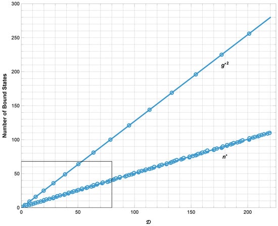
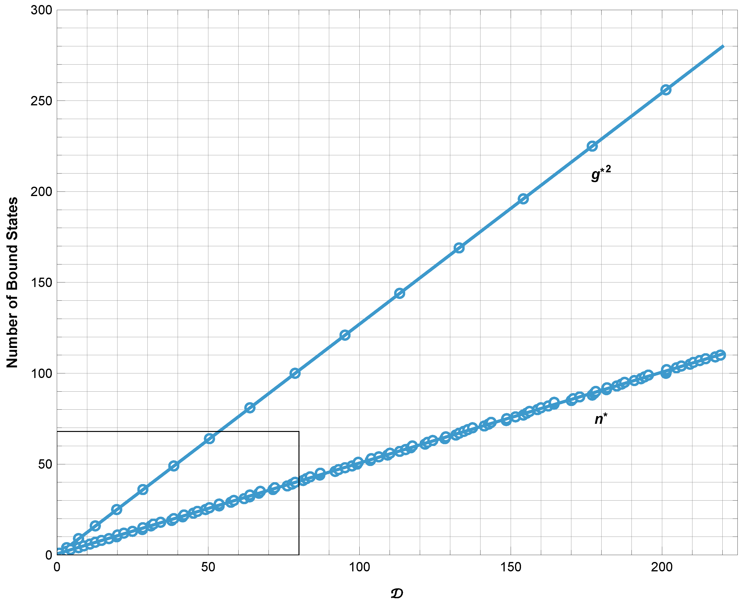
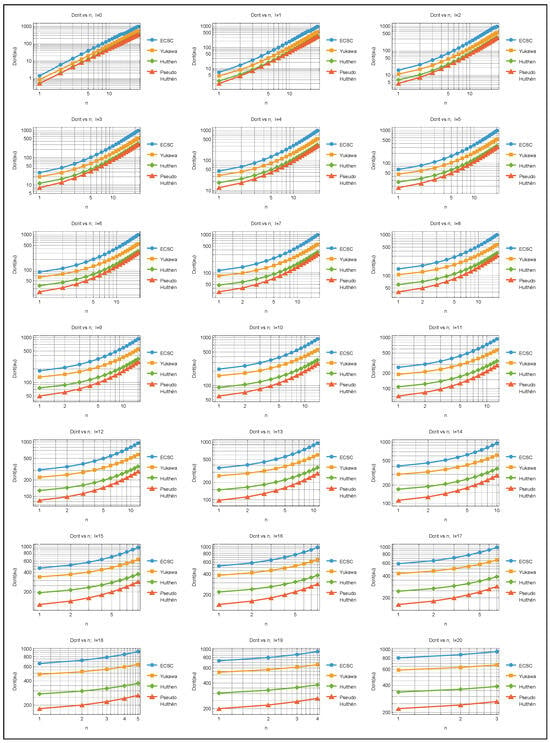
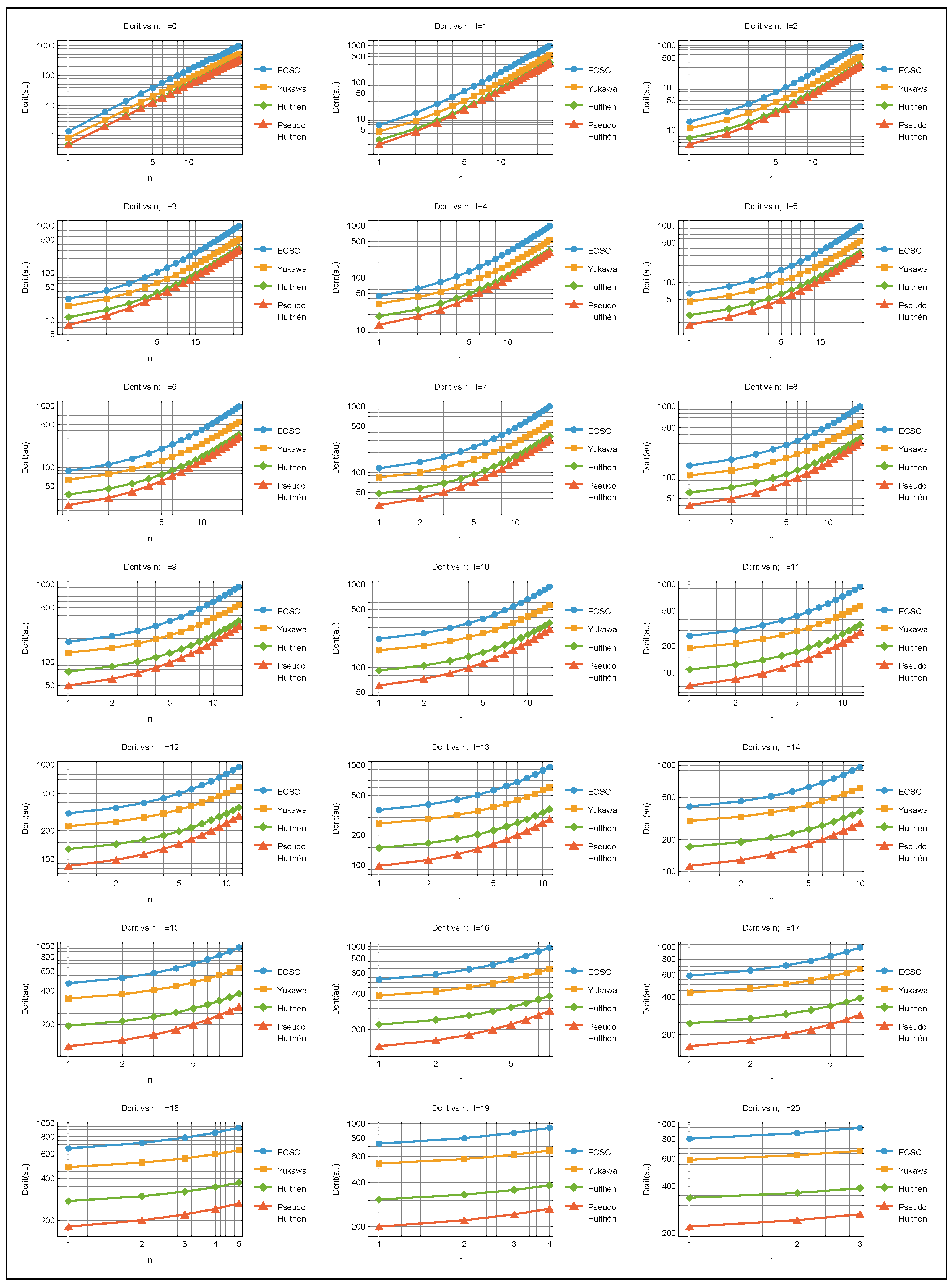
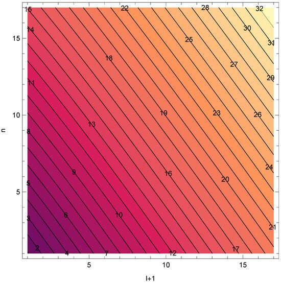
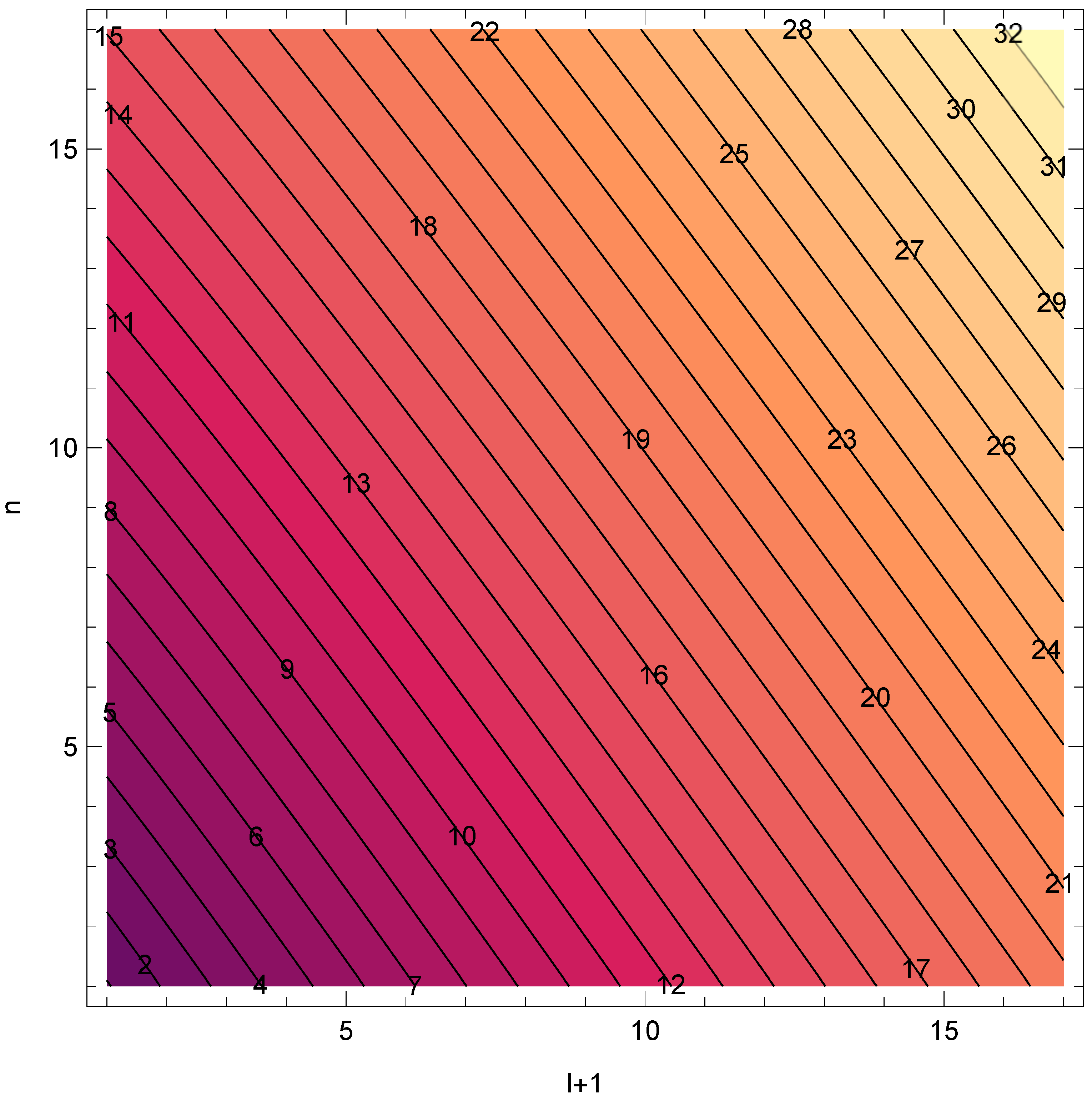
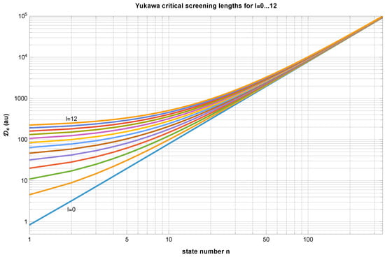
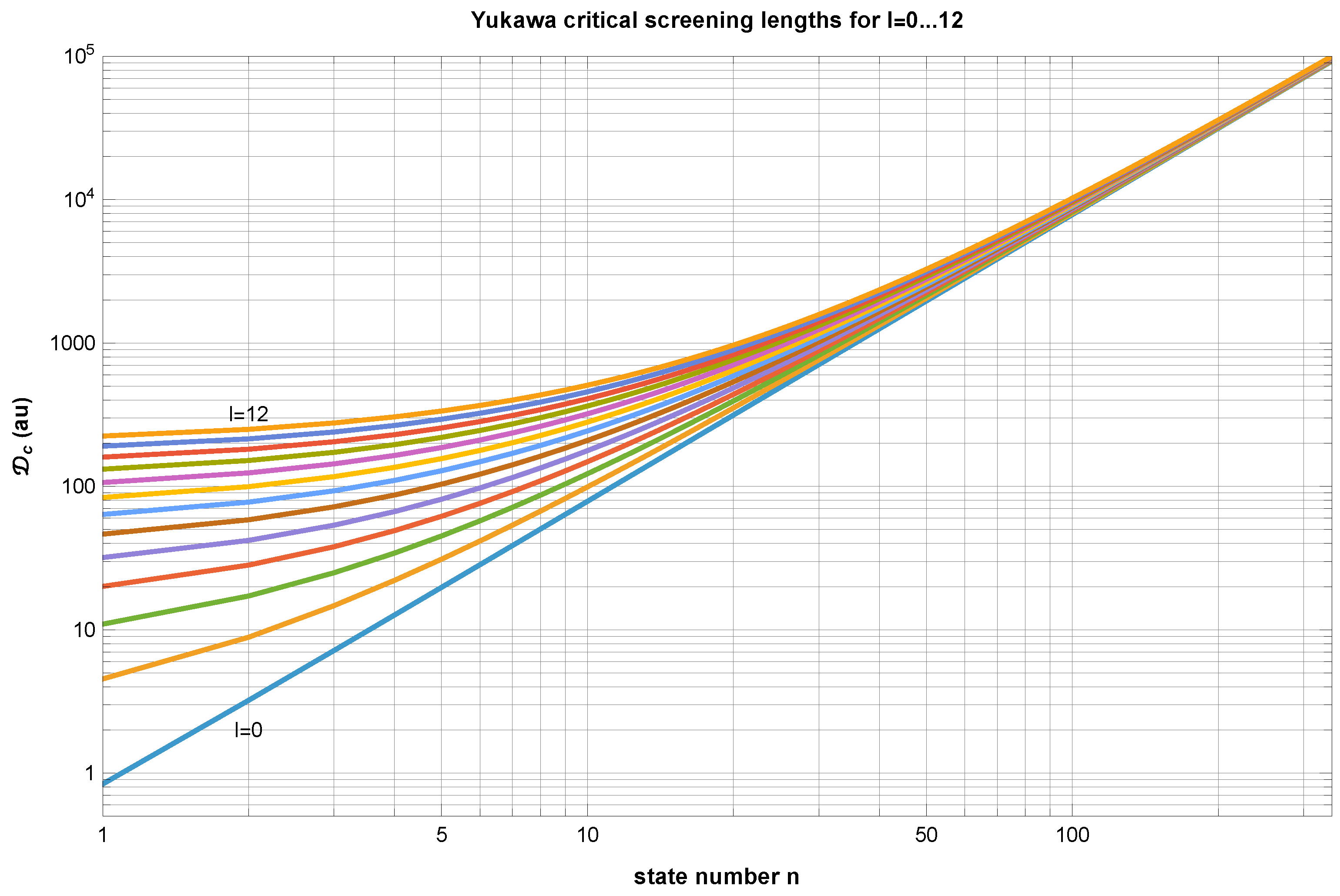
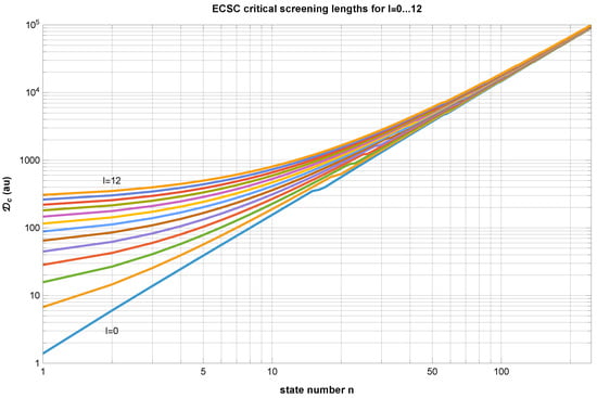
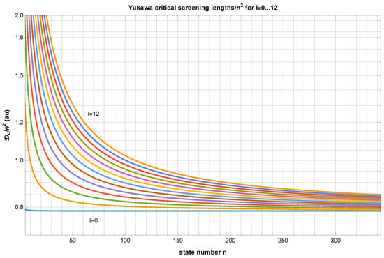
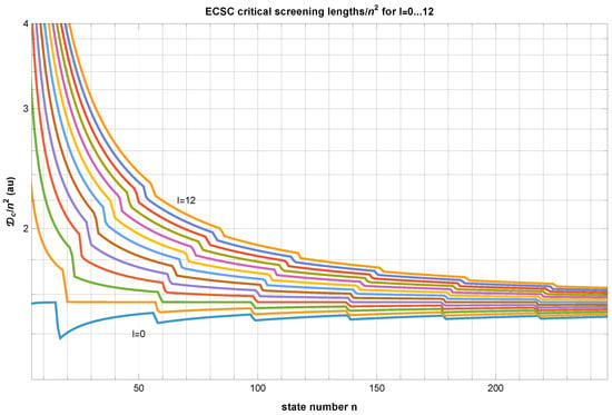
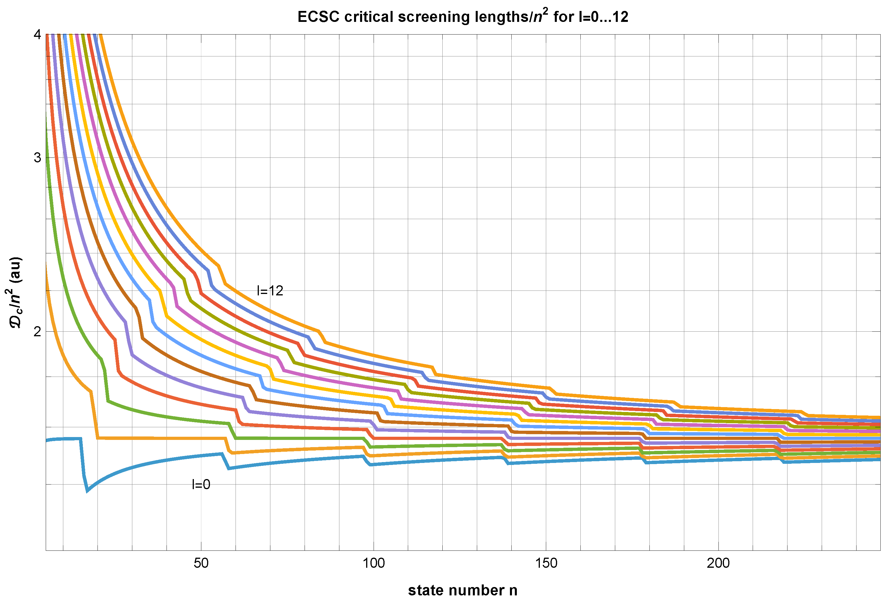
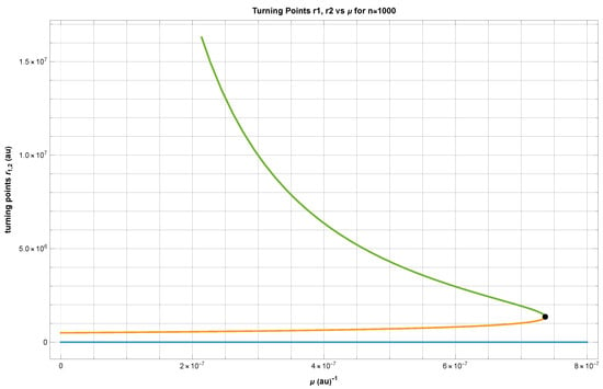
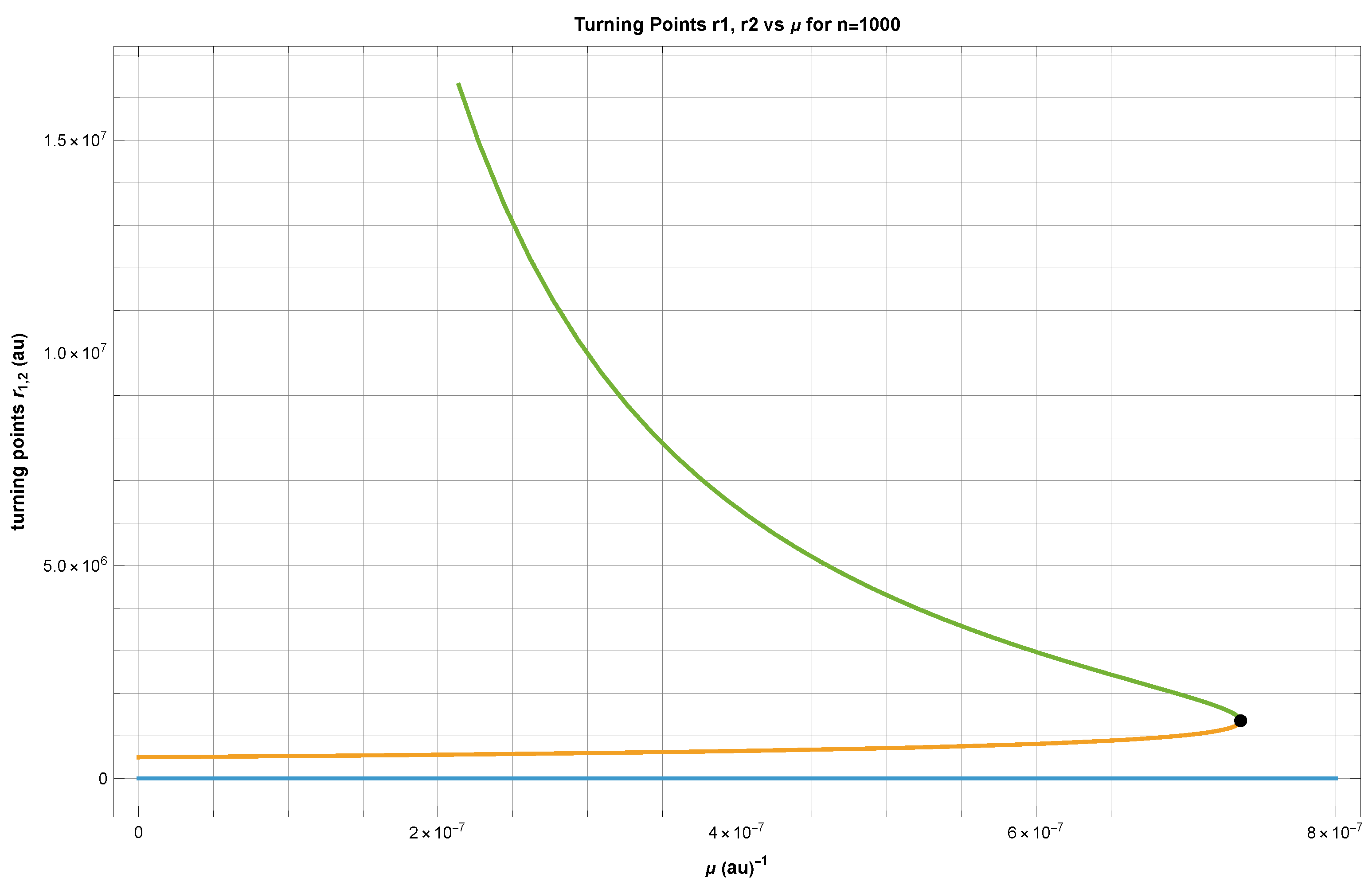
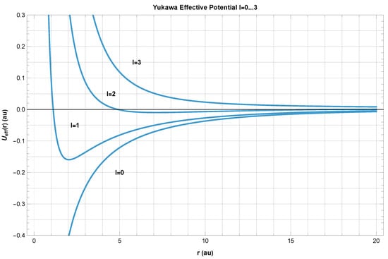
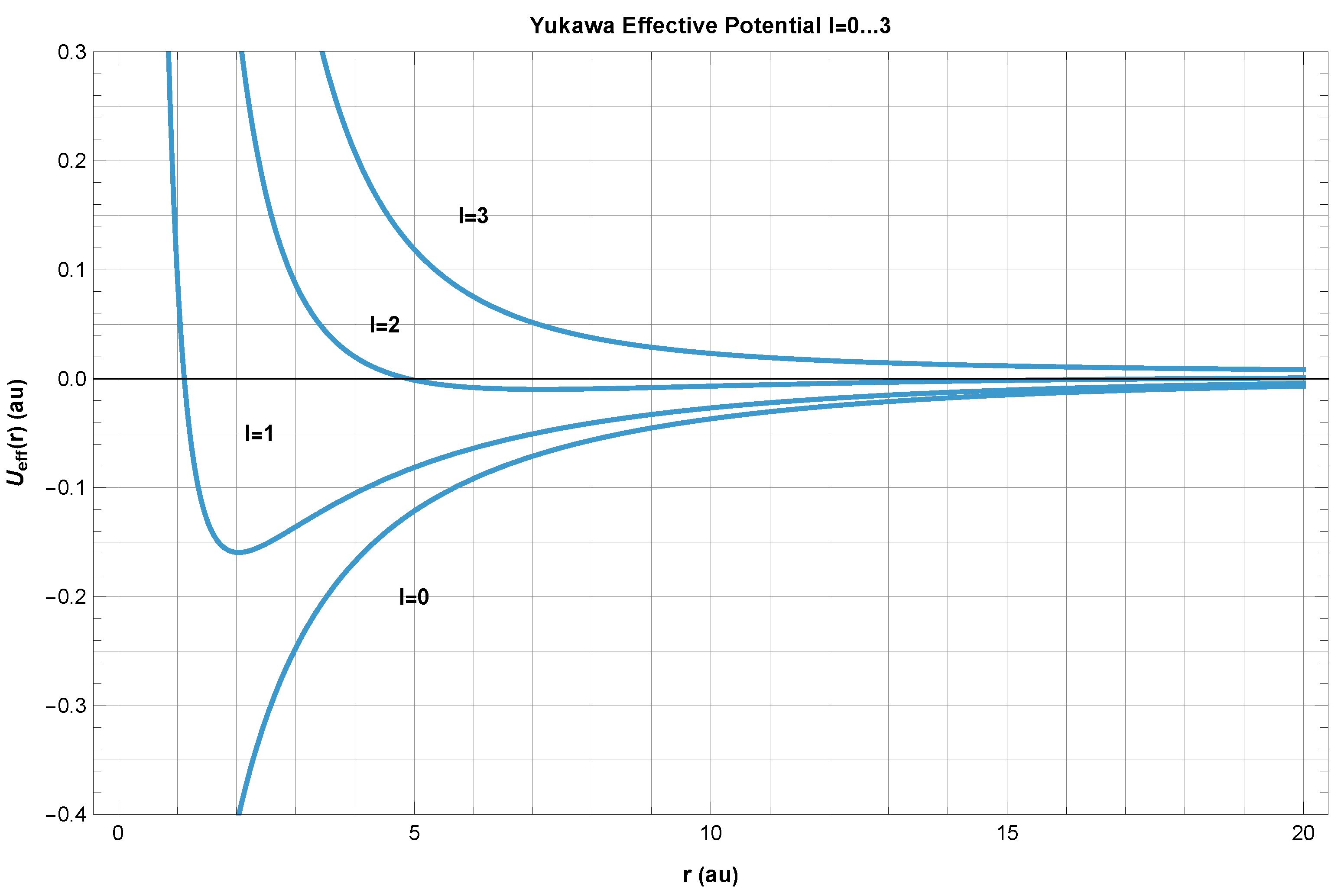

Disclaimer/Publisher’s Note: The statements, opinions and data contained in all publications are solely those of the individual author(s) and contributor(s) and not of MDPI and/or the editor(s). MDPI and/or the editor(s) disclaim responsibility for any injury to people or property resulting from any ideas, methods, instructions or products referred to in the content. |
© 2026 by the author. Licensee MDPI, Basel, Switzerland. This article is an open access article distributed under the terms and conditions of the Creative Commons Attribution (CC BY) license.