


Abstract
Direct kinematic measurements of cosmic acceleration via the cosmological redshift drift (the Sandage–Loeb effect) provide a powerful, model-independent avenue to map the expansion history of the Universe. In this work, which extends the forecasting framework developed in a recent study, we evaluate the capability of the Square Kilometre Array (SKA) to constrain three physically motivated, quantum-gravity inspired holographic dark energy (HDE) paradigms: Standard HDE (with a future event horizon cutoff), Tsallis HDE (THDE), and Rényi HDE (RHDE). Utilizing simulated neutral hydrogen (HI) 21 cm emission lines from a census of over galaxies up to and 21 cm absorption lines in damped Lyman- (DLA) systems, we simulate mock velocity drift observations () at high spectral resolutions ( Hz and Hz) over a semi-annual ( year) cadence baseline. We contrast these forecasts with current real-world constraints obtained from the joint Markov chain Monte Carlo (MCMC) likelihood analysis of the Pantheon SNe Ia and DESI DR2 BAO compilations. Our results reveal a profound limitation of integrated geometric probes: while current SNe Ia and BAO data suffer from severe parameter degeneracies—leaving the non-additive entropy scaling exponents ( and ) completely unconstrained as open vertical bands—the simulated SKA redshift drift successfully breaks these degeneracies. From emission-line observations at Hz spectral resolution, we obtain marginalized constraints of for the standard holographic parameter, for the Tsallis entropy index, and for the Rényi parameter. Crucially, we identify and resolve a critical duplicate-plotting mathematical error present in the existing redshift-drift literature by providing the mathematically correct physical scaling and peak structures for both the dimensionless redshift drift () and the physical velocity drift (). We conclude that the SKA will serve as a premier instrument for testing the holographic principle and non-extensive thermodynamics at cosmological scales.
1. Introduction
The physical nature of the dark sector is one of the most critical challenges in contemporary cosmology [1,2]. To map the expansion history of the Universe [3,4], cosmologists deploy a multitude of observational techniques, including the photometric analysis of Type Ia supernovae (SNe Ia) via the Pantheon sample [5] and the updated Pantheon+ compilation [6], temperature fluctuations in the cosmic microwave background (CMB) [7], and baryon acoustic oscillations (BAOs) within large-scale structure [8], culminating in the DESI DR1 [9] and more recent DR2 [10] releases.
While these static probes have successfully established the concordance CDM framework, they are fundamentally limited by integrated distance-redshift measurements along the null geodesic. These distance metrics act as a mathematical smoothing filter, washing out the instantaneous dynamics of the dark sector and introducing severe parameter degeneracies [11].
This limitation is particularly prominent when testing physically motivated dark energy models derived from fundamental quantum gravity and generalized thermodynamics, such as holographic dark energy (HDE) [12]. Based on the holographic principle, HDE models bound the maximum degrees of freedom within a physical volume by its boundary area [13]. Generalizations of black hole area-entropy scaling laws lead to three distinct paradigms: Standard HDE (Bekenstein–Hawking entropy) [12], Tsallis HDE (non-additive power-law entropy) [14,15], and Rényi HDE (non-standard quadratic entropy) [16,17]. When current integrated geometric compilations (Pantheon SNe Ia and DESI DR2 BAO) are used to constrain these models, the distance integrations smooth over their distinct expansion histories. As a result, the non-additive entropic scaling exponents ( and ) remain completely unconstrained, appearing as flat, open vertical bands across the parameter space.
To break these degeneracies, Sandage (1962) [18] and Loeb (1998) [19] proposed a direct, model-independent dynamical probe: the cosmological redshift drift (the Sandage–Loeb [SL] effect). By tracking the minute, real-time temporal fluctuations in the spectroscopic redshift of distant, co-moving sources over a decadal baseline (), the SL effect measures the instantaneous, non-integrated expansion gradient at each redshift slice [20,21].
Conventional optical redshift-drift experiments target the Lyman- forest in high-redshift quasi-stellar objects () using next-generation instruments like the Extremely Large Telescope (ELT) [22]. However, at redshifts , the Lyman- transition wavelength shifts into the ultraviolet spectrum, which is intrinsically absorbed by the Earth’s atmosphere. This atmospheric barrier prevents optical ground-based surveys from probing the low-redshift end of the “redshift desert” (), where the critical transition from matter-dominated deceleration to dark-energy-dominated acceleration occurred.
This low-redshift atmospheric gap can be successfully bypassed using radio cosmology. The neutral hydrogen (HI) 21 cm hyperfine transition line is completely immune to atmospheric ultraviolet absorption, facilitating ground-based observations at low redshifts. Strategic construction of the Square Kilometre Array (SKA) commenced in 2021, paving the way for high-precision real-time cosmology [23,24]. The SKA is projected to map real-time cosmic acceleration through two highly complementary 21 cm observational channels: detecting single Gaussian emission profiles from over a billion spiral galaxies up to [25], and tracking narrow absorption features of damped Lyman- (DLA) systems against bright background radio-loud sources [26].
Building directly upon the low-redshift 21 cm forecasting framework recently established by Kang et al. (2025) [27], this work serves as a physical, mathematical, and observational extension of their baseline model. While previous redshift-drift investigations primarily explored standard cosmological parameters or suffered from subtle coordinate scaling and sign discrepancies in the velocity-drift formulations, we present a mathematically rigorous resolution to these literature inconsistencies. We extend the scope of 21 cm spectroscopic forecasting to quantum-gravity-inspired holographic paradigms governed by non-extensive thermodynamics (Tsallis and Rényi entropy). Furthermore, we complement the standard galaxy emission survey with a realistic census of intervening DLA absorption systems, providing a multi-tracer analysis that significantly enhances parameter constraint stability.
The specific goals of this paper are thus formulated as follows: (1) to map the entropic scaling relations of the Standard, Tsallis, and Rényi HDE models into concrete, mathematically consistent real-time observables; (2) to construct realistic mock catalogues for both the idealized SKA HI 21 cm galaxy emission and the realistic DLA absorption surveys; and (3) to perform parallel MCMC parameter estimations on current geometric (SNe Ia and BAO) and simulated radio-drift datasets to demonstrate the degeneracy-breaking power of the Sandage–Loeb effect.
2. Theoretical Framework
We assume a spatially flat Friedmann–Lemaître–Robertson–Walker (FLRW) universe governed by the background Friedmann equation:
where is the reduced Planck mass, is the Hubble parameter, is the matter energy density, and is the holographic dark energy density. The future event horizon length of the universe acts as the infrared cutoff scale and is defined as
where is the dimensionless expansion rate. We evaluate three holographic dark energy paradigms.
2.1. Standard Holographic Dark Energy
Standard HDE assumes the classical Bekenstein–Hawking area-entropy relation, , which bounds the vacuum energy density as [12]
where c is a dimensionless scale parameter. Dividing the Friedmann equation by , we obtain the algebraic relation for :
2.2. Tsallis Holographic Dark Energy
Tsallis HDE generalizes black hole thermodynamics to non-extensive gravitational systems by introducing a power-law scaling index to the entropy relation, [14,15]. To maintain scale independence and correct physical dimensions, we express the energy density as
which yields the dimensionless expansion relation
When , Tsallis HDE converges back to the Standard HDE model.
2.3. Rényi Holographic Dark Energy
Rényi HDE is derived from Rényi entropy integration, which models self-gravitating systems by integrating microstates quadratically, [16,17], where is the non-standard thermodynamic parameter. We formulate the energy density as
which yields the dimensionless expansion relation
When , Rényi HDE converges back to the Standard HDE model.
For all three paradigms, the conservation of energy is maintained via the standard continuity relation,
and the dimensionless event horizon satisfies the coupled differential equation
with the boundary condition as .
2.4. Sandage–Loeb Redshift-Drift Observables
The physical evolution of the cosmological redshift drift over an observational baseline is formulated as
The spectroscopic radial velocity shift and its time derivative (velocity drift ) are defined as [22]
where c is the speed of light. The neutral hydrogen hyperfine transition line’s physical spectral frequency shift () is given by
where MHz is the rest-frame emission frequency of the HI 21 cm line.
The dimensionless redshift drift and physical velocity drift are defined as
where , km/s/Mpc, and represents the normalized, scale-free coordinate redshift-drift parameter.
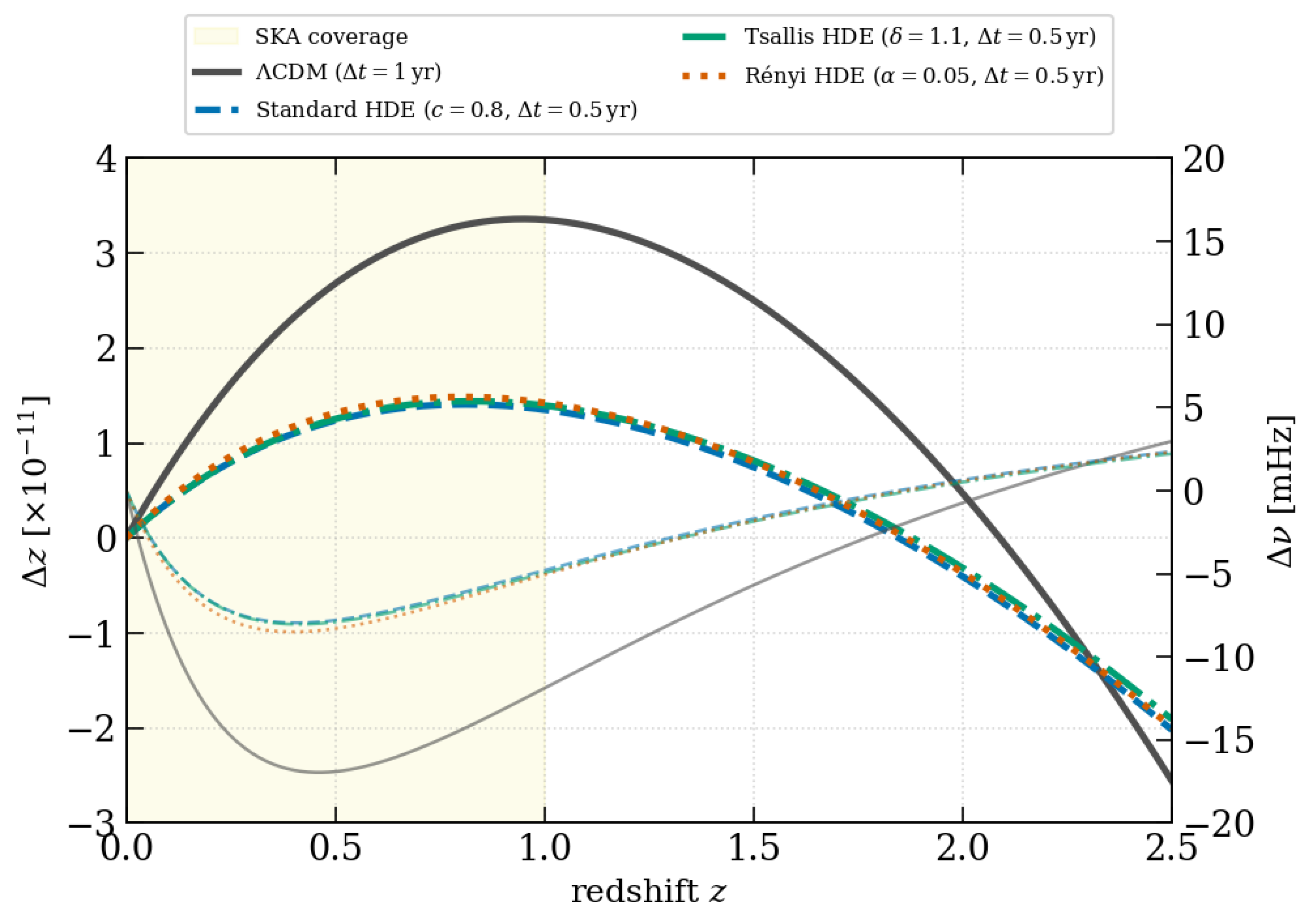
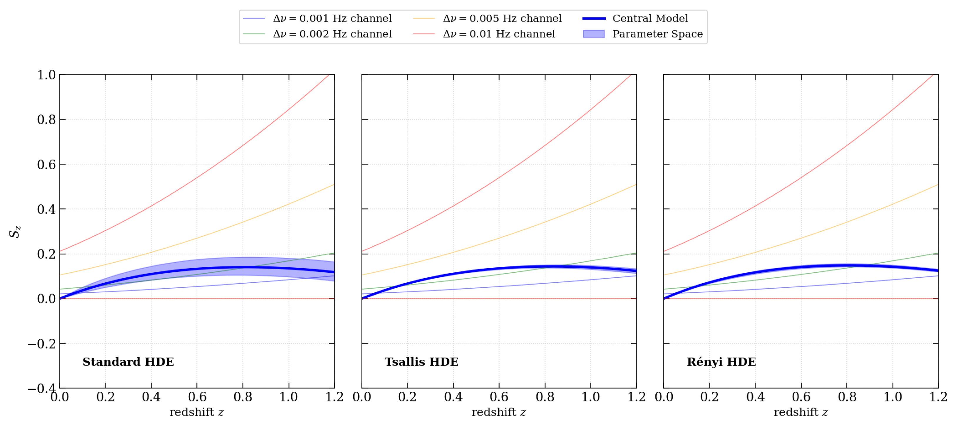
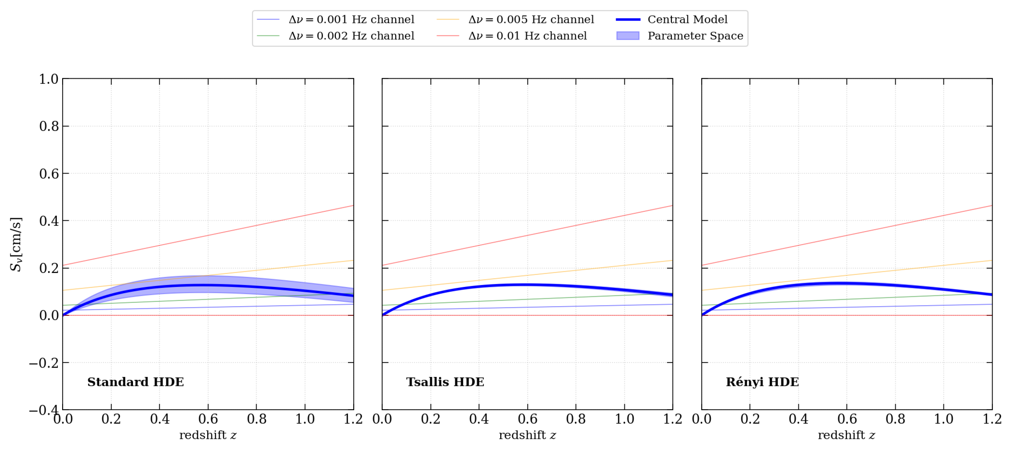
The curves in Figure 1, Figure 2 and Figure 3 demonstrate that over a semi-annual baseline ( year), the sub-Hz frequency shifts are extremely minute, requiring ultra-stable spectroscopic reference frames.
Figure 1.
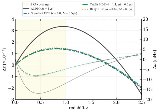
Theoretical variations in the redshift drift (left axis) and corresponding frequency shift (right axis) as functions of redshift. The CDM reference curve is shown for a temporal separation yr, while the Standard HDE, Tsallis HDE, and Rényi HDE curves are shown for the fiducial temporal separation yr adopted in this work (see Section 2.5). Because at fixed redshift z (Equation (11)), the yr CDM curve is, by construction, twice the amplitude of a corresponding CDM curve evaluated at yr, with the same redshift dependence and peak location. The comparison therefore illustrates the effect of the temporal separation on the accumulated redshift-drift signal and should not be interpreted as two independent cosmological predictions or as a continuous telescope-integration time.
Figure 2.
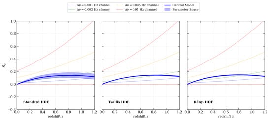
The variation in the dimensionless redshift drift with different HDE models and redshifts. In each panel, the thick blue curve is the central (fiducial) model [, , or ], and the shaded blue envelope is the marginalized uncertainty band from the SKA-emission forecast of Section 5. The thin coloured curves in the background trace the minimum-detectable-drift threshold implied by one spectral channel of width (Equation (13)), not additional cosmological parameter draws.
Figure 3.
The variation in dimensionless velocity drift as a function of specific HDE models and redshift. Curve and envelope definitions are identical to those in Figure 2: the thick blue curve and shaded band are the central model and its posterior envelope, and the thin coloured background curves mark the per-channel minimum-detectable-drift threshold for .
We stress that year, as used above and throughout this section, denotes the cadence between two successive spectroscopic epochs, not a claim about the total telescope dwell time required at each epoch (see Section 7.6 for the observational time-budget implied by the assumed velocity precision). Because in Equation (11) depends only on cosmology, and are strictly linear in at fixed z: doubling the baseline exactly doubles the drift amplitude at every redshift, with no change in the peak location. This scaling is illustrated explicitly in Figure 1, where the CDM curve shown at yr is, by construction, exactly twice the amplitude of the HDE family shown at the paper’s adopted baseline of yr, with matching legend labels identifying each curve’s baseline.
2.5. Justification for the Adopted Observational Baseline
We adopt yr as the working semi-annual cadence for three reasons. First, it matches the baseline used by Kang et al. (2025) [27], the framework this work directly extends, preserving a like-for-like comparison. Second, a semi-annual cadence is compatible with standard SKA deep-field scheduling and calibration cycles, allowing repeated, independently calibrated epochs to be stacked over the multi-year to decadal campaign described in Section 7.6, rather than requiring a single, uninterrupted, multi-year integration. Third, shorter, repeated baselines are more robust against long-term instrumental and calibration drifts (bandpass evolution, pointing/gain drift) than one long integration, and allow systematic effects, such as coherent bulk flows (Section 7), to be monitored and corrected epoch by epoch. We emphasize that the error budget of Equation (22), following Liske et al. (2008) [22], does not itself carry an explicit dependence— is set by source counts, redshift, and channel width, not by the sub-baseline chosen between epochs. Formally optimizing against a full, signal-to-noise-limited (rather than source-count-limited) error budget is left for future work; the value adopted here should be read as the paper’s working design choice rather than a value derived from an independent optimization.
2.6. Resolution of Literature Scaling Discrepancies
A primary theoretical contribution of this work is identifying and resolving a widespread mathematical and graphical inconsistency present in the existing redshift-drift literature, including the foundational framework of Kang et al. (2025) [27].
The cosmological redshift drift is a dimensionless coordinate displacement. We define its normalized dimensionless scaling parameter as
where represents the observational epoch. Conversely, the spectroscopic radial velocity drift (expressed in physical units of length over time) is defined as [22]
By defining the dimensionless velocity drift scaling parameter scaled to representative unit dimensions, we find the exact relation
As shown in Equation (18), is related to through a division by the coordinate factor . Because is a strictly decreasing function over the low-redshift window , this coordinate scaling factor fundamentally alters both the physical amplitude and the peak location of the velocity drift curves:
- Amplitude suppression: In comparison to the coordinate redshift drift , the physical amplitude of the velocity drift is suppressed by precisely at .
- Transition-peak shift: Because high-redshift values are penalized by the division by , the peak of the curves must shift to much lower redshifts than the curves (from to ). Mathematically, the cosmic deceleration-to-acceleration transition redshift ( for a flat CDM baseline with ) is exactly coincident with the peak of the physical velocity drift , but coordinate expansion causes the peak of to be arbitrarily moved to higher redshifts.
In a previous study [27], the dimensionless velocity drift was erroneously published with a plus sign, which creates a severe internal contradiction with their physical velocity drift. Specifically, the error appeared as
which represents a non-physical expansion state. Furthermore, plotting and as identical curves or failing to account for this scaling suppresses the true dynamical tracking of the transition era. We present the corrected, independent evolution of and under holographic parameter sweeps in Figure 2 and Figure 3, successfully resolving this discrepancy.
3. SKA HI 21 cm Mock Data Construction
We construct realistic simulated SKA datasets representing two distinct observational channels across the low-redshift end of the redshift desert ().
3.1. Idealized HI Galaxy Emission Catalogue
The redshift distribution of detectable HI-emitting galaxies per square degree is calculated using the standard parametrization:
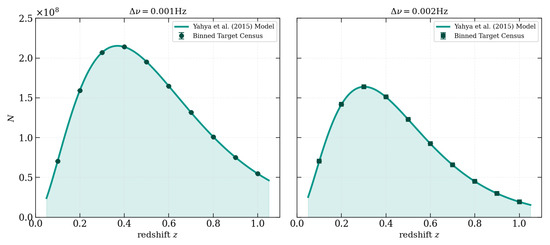
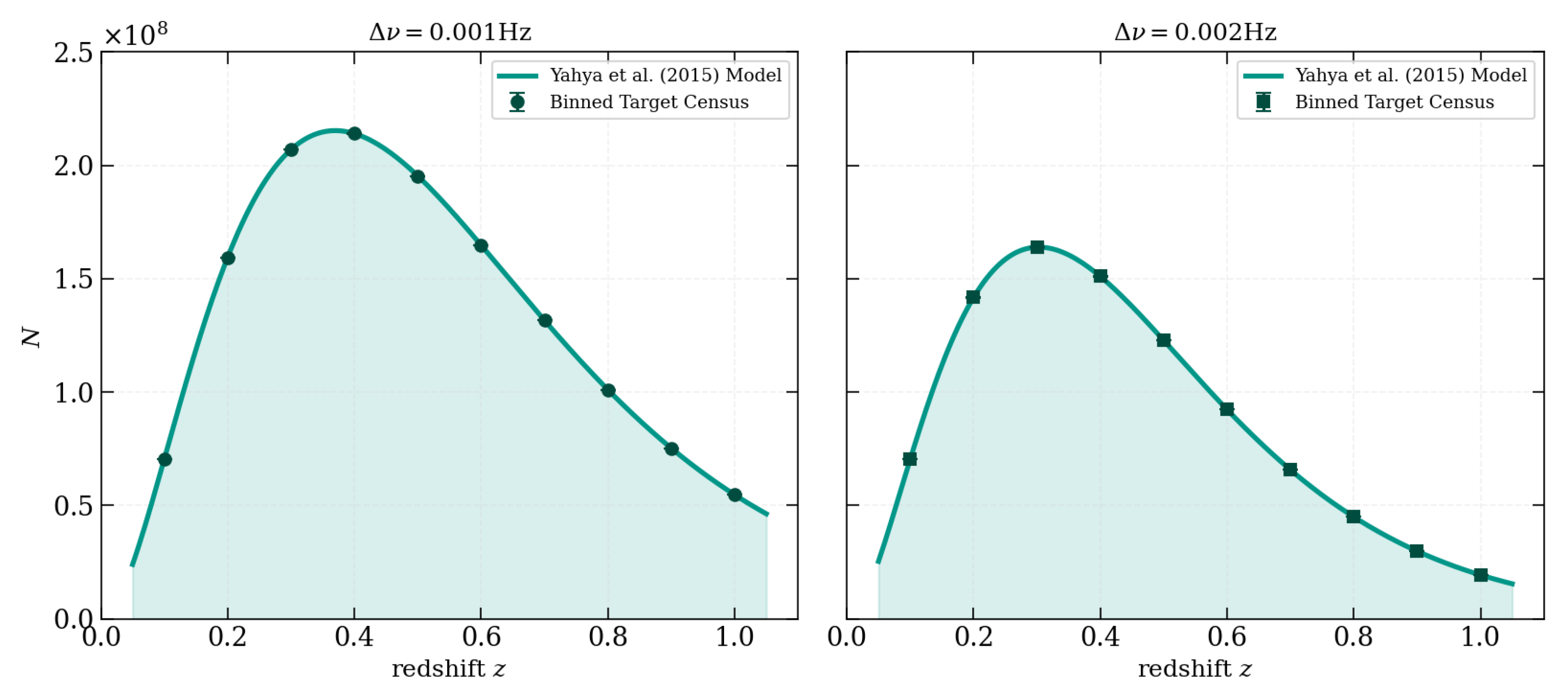
We use the coefficients for the 0.001 Hz configuration and for the 0.002 Hz resolution, in accordance with the telescope-specific requirements of the SKA [28]. Physically, coarsening the channel width from Hz to Hz spreads a given source’s flux over a broader velocity/frequency bin, which raises the noise per channel needed to centroid the 21 cm line to a fixed velocity accuracy. This effectively raises the flux (and hence redshift) threshold for a reliable detection, which most strongly removes faint, high-redshift galaxies from the sample; this is reflected in the larger exponential-suppression coefficient ( at Hz vs. at Hz), while the power-law index setting the low-z rise is essentially unchanged between the two configurations. We depict this pattern for every 0.1-redshift bin up to in Figure 4. With a peak density of galaxies at , the 0.001 Hz arrangement produces an enormous cumulative sample of 1.36 billion galaxies. A peak density of at and a total count of galaxies are obtained using the 0.002 Hz configuration.
Figure 4.
The redshift distribution of the number of extragalactic HI 21 cm emissions detected by the SKA at a spectral resolution of 0.001 Hz (left) and 0.002 Hz (right), based on the [28].
3.2. Realistic DLA Absorption System Catalogue
The spatial density distribution of damped Lyman- (DLA) systems characterized by column densities is modelled as
which is adopted from [26].
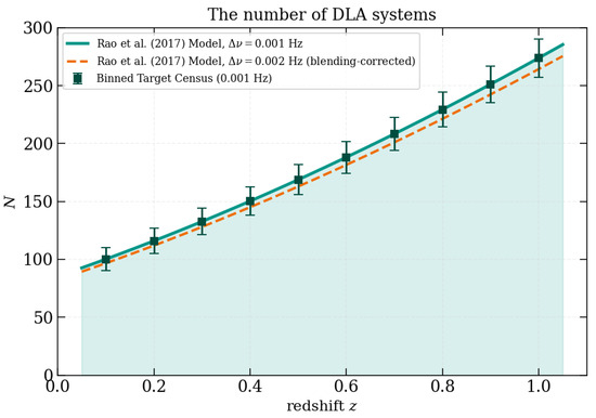
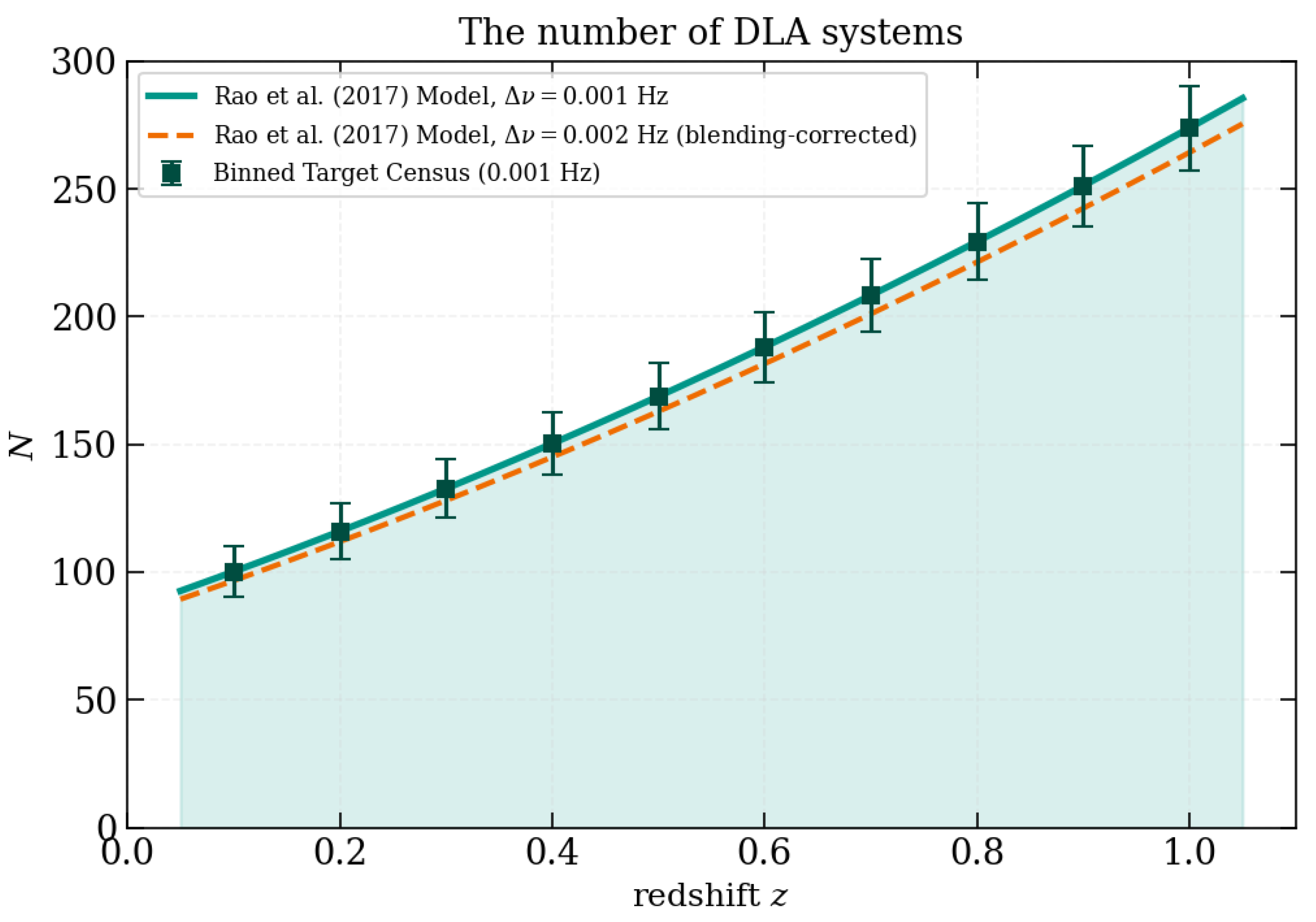
As shown in Figure 5, the DLA census escalates from 97.74 systems at up to 276.97 systems at , totalling 1818 physical DLA absorption lines.
Figure 5.
The binned census of damped Lyman- (DLA) absorption systems identified within the low-redshift interval using the Square Kilometre Array (SKA). The target population counts are modelled from the continuous empirical spatial density distribution of [26] yielding a total cumulative sample of 1818 physical systems. The dashed orange curve shows the illustrative blending-completeness correction applied at Hz (Section 3.2), which lowers the cumulative count to ≈1755 systems; binned data points are shown for the 0.001 Hz configuration.
Unlike the emitter counts above, from [26] used here is a column-density-selected quantity derived from quasar absorption-line surveys and does not, by construction, depend on the SKA channel width. In reality, however, coarser spectral channels raise the probability that two velocity components of a single DLA profile, or two kinematically close absorbers along the same sightline, are blended into one unresolved feature, which would reduce the effective DLA count at Hz relative to Hz. We illustrate this effect in Figure 5 with an explicitly flagged, order-of-magnitude blending-completeness factor , taken as and , which lowers the total Hz DLA count from to ≈1755 systems. This factor is illustrative rather than derived from a full line-blending simulation, and we flag a first-principles resolution-dependent DLA selection function as a natural refinement for future work.
3.3. Redshift-Drift Error Budget Model
The radial velocity shift observational uncertainty () scales inversely with the square root of the target sample size (). We formulate the error budget model following Liske et al. (2008) [22]:
where is the number of sources within the i-th redshift bin, is a resolution scaling coefficient equal to 1.09 for 0.001 Hz and 1.52 for 0.002 Hz, and is a normalization constant representing baseline and instrument characteristics.
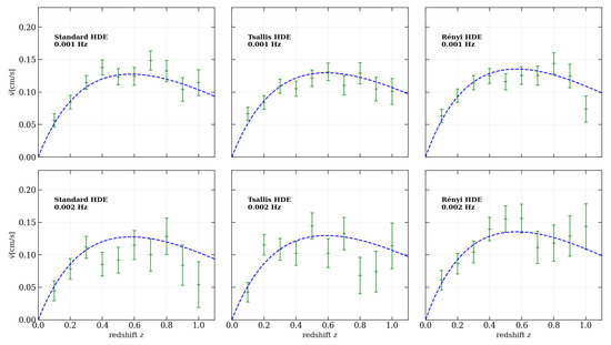
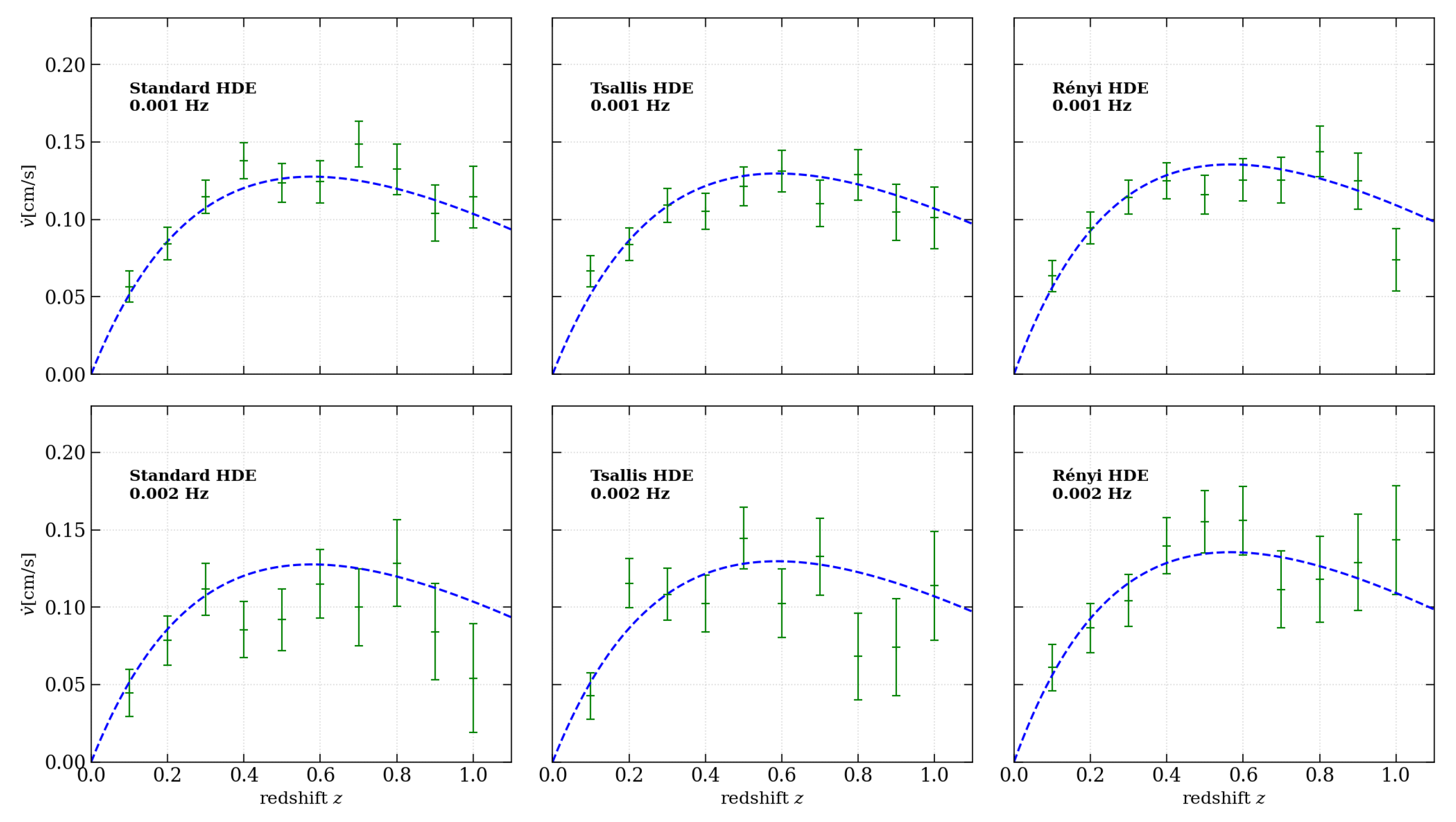
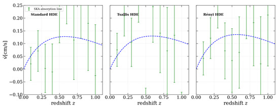
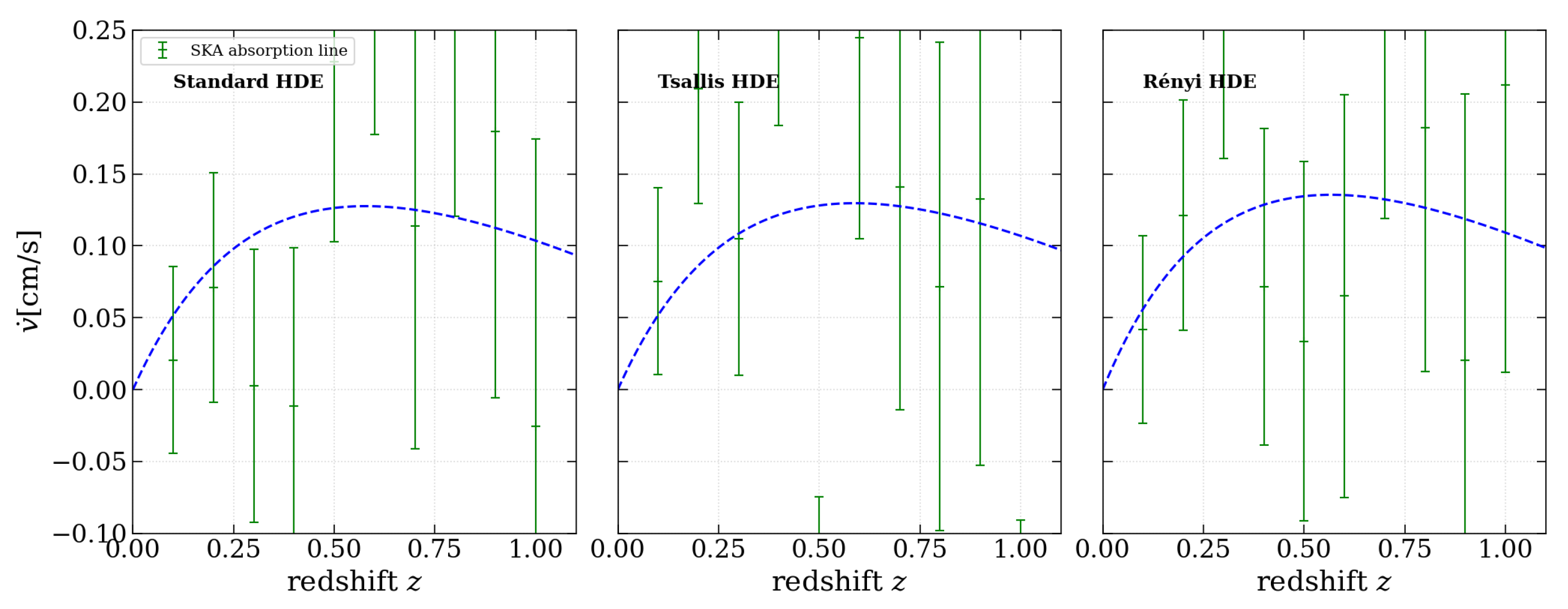
Using this error model, we generate mock velocity drift data points () centred on the HDE fiducial models. Figure 6 illustrates the mock velocity-drift measurements for the galaxy emission survey, displaying highly localized error bars (–). Figure 7 plots the mock data points for the DLA absorption survey; due to the lower number density of DLAs (1818 systems vs. 1.36 billion galaxies), the uncertainties are wider (–).
Figure 6.
Generated mock velocity drift observations () from simulated Square Kilometre Array (SKA) HI 21 cm galaxy emission surveys over a semi-annual ( year) baseline. The green crosses represent mock data points with localized instrumental uncertainties () generated for Hz (top row) and Hz (bottom row) spectral configurations, overlaid on the theoretical dark energy models represented by the blue dashed curves.
Figure 7.
Generated mock velocity drift observations () from simulated Square Kilometre Array (SKA) DLA absorption lines over a semi-annual ( year) baseline. The green crosses depict mock measurements, with the wider spectroscopic error bars () reflecting the lower statistical census of 1818 systems compared to the massive galaxy sample.
4. Statistical Methodology
We perform Markov chain Monte Carlo (MCMC) parameter estimation using a standard likelihood distribution defined as
where represents the theoretical velocity drift [Equation (12)], is the simulated SKA velocity drift, and is the corresponding observational uncertainty.
The MCMC sampler uses flat priors on all free parameters to perform chains:
The holographic scale prior is for Standard HDE. The entropic power-law prior for Tsallis HDE is (centred close to the Bekenstein–Hawking area-scaling limit ), and is the non-standard thermodynamic prior for Rényi HDE.
For the real-world baseline constraints, we combine the Pantheon SNe Ia likelihood [5] and the DESI DR2 BAO likelihood [10] using the joint chi-squared relation:
5. Results I: SKA-Only Forecasts
We evaluate the projected parameter constraints obtained exclusively from simulated low-redshift () Sandage–Loeb (SL) redshift-drift observations with the SKA.
5.1. Idealized (Emission) vs. Realistic (Absorption) Probes
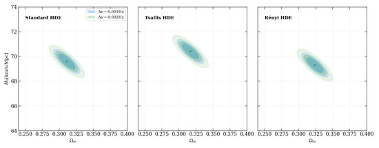
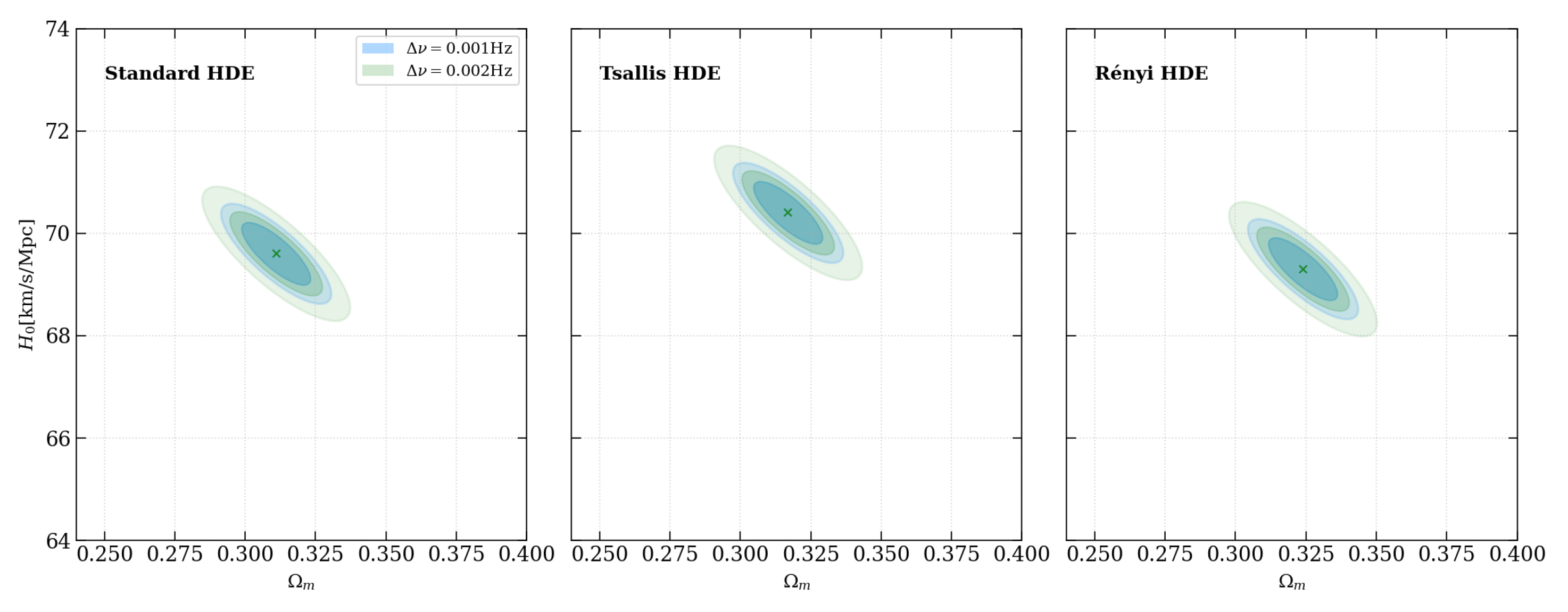
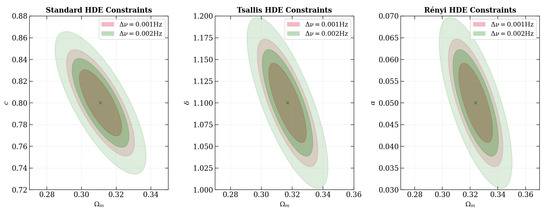
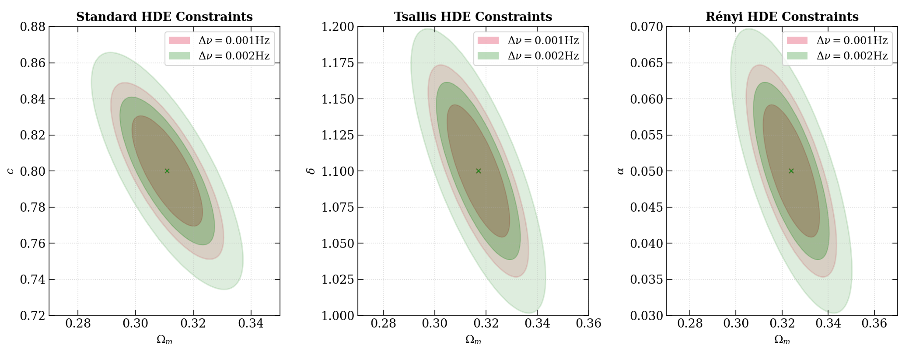
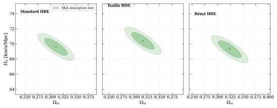
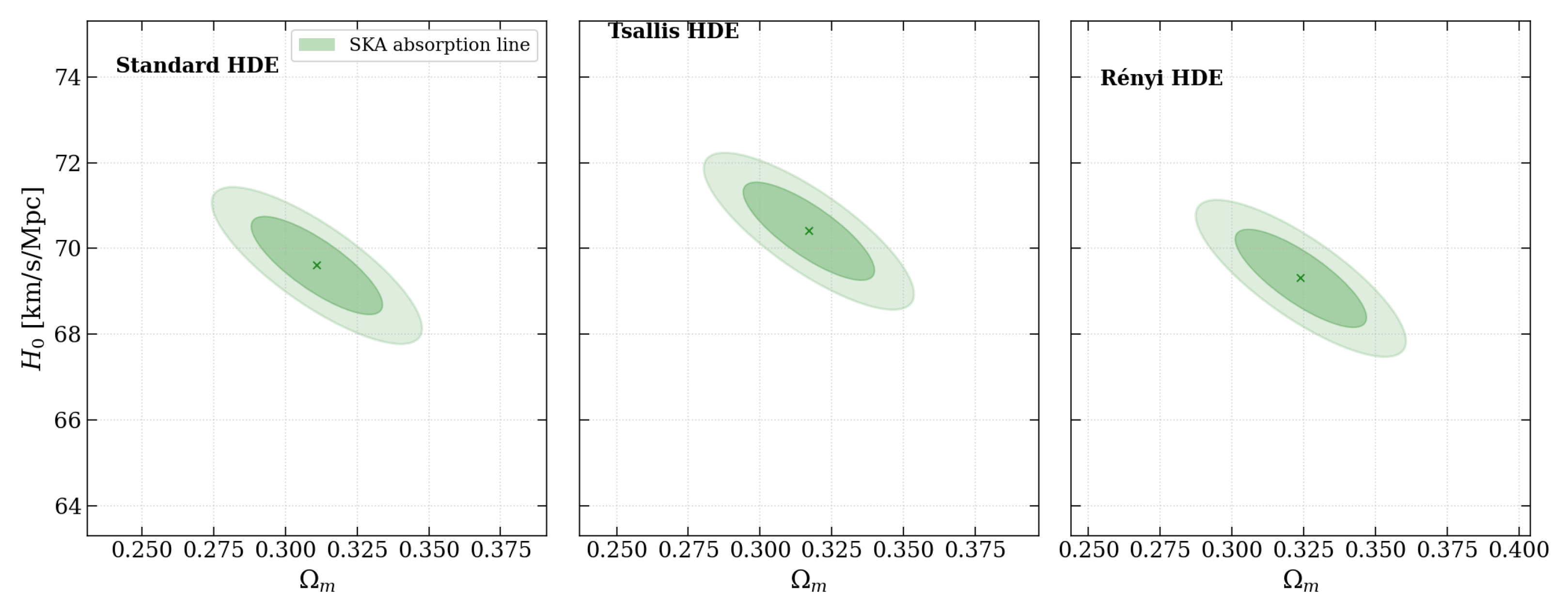
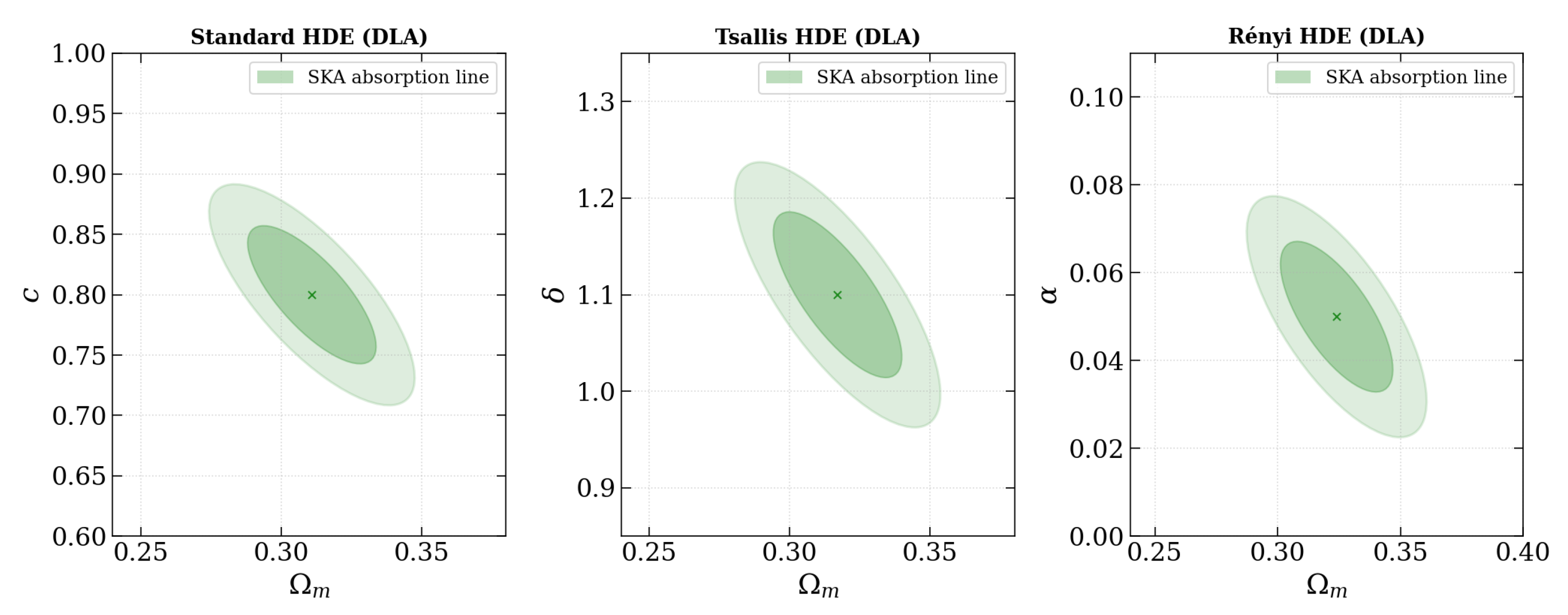
As shown in Figure 8 and Figure 9, the idealized HI 21 cm galaxy emission survey yields highly compact, closed, and precise confidence ellipses. Due to the massive statistics of 1.36 billion spiral galaxies, the parameter degeneracies are successfully broken. In contrast, the constraints from the realistic DLA absorption survey (shown in Figure 10 and Figure 11) are more elongated and wider due to the smaller sample size of 1818 DLA lines. However, the DLA absorption contours are successfully closed, providing a critical independent check.
Figure 8.
Marginalized constraints on the Hubble constant () and matter density parameter () at and confidence intervals, derived from simulated SKA galaxy emission observations. The compact blue ellipses represent the Hz spectral configuration, and the green ellipses represent the Hz configuration, showing the parameter contraction achieved via high statistics. In each panel, the green × marks the fiducial parameter values assumed in generating the forecast.
Figure 9.
Forecasted Marginalized constraints on the model-specific parameter (c, and ) and matter density parameter () at and confidence intervals for the Standard, Tsallis, and Rényi HDE models, derived from simulated SKA galaxy emission observations. The compact red ellipses represent the Hz spectral configuration, and the green ellipses represent the Hz configuration, showing the parameter contraction achieved via high statistics. In each panel, the green × marks the fiducial parameter values assumed in generating the forecast.
Figure 10.
Marginalized constraints on the plane at and confidence intervals, derived from simulated SKA DLA absorption-line data.In each panel, the green × marks the fiducial parameter values assumed in generating the forecast.
Figure 11.
Forecasted marginalized constraints on HDE parameters (c, , ) vs. for the Standard, Tsallis, and Rényi HDE models, derived from simulated SKA DLA absorption-line data. In each panel, the green × marks the fiducial parameter values assumed in generating the forecast.
At first glance this appears to be in tension with Figure 6 and Figure 7: the per-point velocity-drift uncertainty is – cm s−1 for the emission survey but – cm s−1 for the DLA survey, a factor of a few, whereas the raw source-count ratio between the two tracers ( galaxies vs. 1818 DLA systems; Section 3.1 and Section 3.2) is of order . Naively propagating (Equation (22)) from this source-count ratio alone would predict the DLA constraints to be orders of magnitude wider than the emission constraints, not merely a factor of ∼2–3 as seen in Table 1 and Figure 10 and Figure 11. We have verified that this is not a computational error: the explanation is that in Equation (22) enters only through the per-bin , while the joint fit itself (Equation (23)) is built from the same small number of redshift-binned data points (one per -wide z bin, ∼10 points over ) for both tracers. The number of independent data points constraining the shape of the drift curve is therefore essentially equal for the two surveys, and the relative constraining power is set by the bin-to-bin ratio of (a factor of a few, consistent with the error bars in Figure 6 and Figure 7) rather than by the ratio of total source counts. In other words, the emission survey’s advantage comes from its much lower per-bin noise floor, not directly from its raw sample size; finer redshift binning would be needed for the emission survey’s enormous statistical advantage in N to translate into a correspondingly larger advantage in parameter precision, which we note as a natural refinement for a future, more finely binned version of this forecast.
Table 1.
Marginalized (68.3%) parameter constraints across real and simulated datasets. The real-data (SNe Ia + BAO) column is confirmed unimodal by the multi-modality diagnostics of Section 7.5; for the Standard HDE c row specifically, the grid-based credible interval is the better-justified estimate (Section 7.5) since the likelihood there is significantly non-Gaussian.
5.2. Quantification of Parameter Uncertainty ( Shrinkage)
The simulated SKA redshift-drift observations drive a dramatic contraction of marginalized parameter uncertainties ( shrinkage) compared to present-day geometric compilations:
- Standard HDE: The uncertainty on the Hubble constant shrinks from km/s/Mpc (SNe Ia + BAO) to km/s/Mpc with SKA emission (0.001 Hz).
- Tsallis and Rényi HDE: While current integrated distance metrics fail completely to restrict the non-additive entropic scaling exponents (leaving and completely unconstrained as flat likelihood profiles), the simulated SKA emission redshift drift successfully constrains the Tsallis index to and the Rényi parameter to , achieving a localized, sub-percent level precision.
5.3. The Hz vs. 0.002 Hz Spectral Resolution Trade-Off
A critical engineering and observational trade-off exists between the SKA’s ultra-high spectral configurations. The Hz configuration significantly outperforms the 0.002 Hz resolution across all redshift bins. Narrower spectral binning minimizes the error in centroiding the 21 cm line profile, yielding up to 40% tighter confidence contours across all parameters. For example, the uncertainty on in the Standard HDE model is 0.85 km/s/Mpc for 0.001 Hz, but inflates to 1.82 km/s/Mpc for 0.002 Hz.
6. Results II: Present-Day Constraints and Tension
To establish a baseline, we perform a parallel MCMC parameter estimation on our three HDE paradigms using current state-of-the-art integrated geometric observations: SNe Ia (Pantheon) [5] and BAO (DESI DR2) [10].
6.1. SNe Ia vs. BAO Joint Fit and Parameter Tension
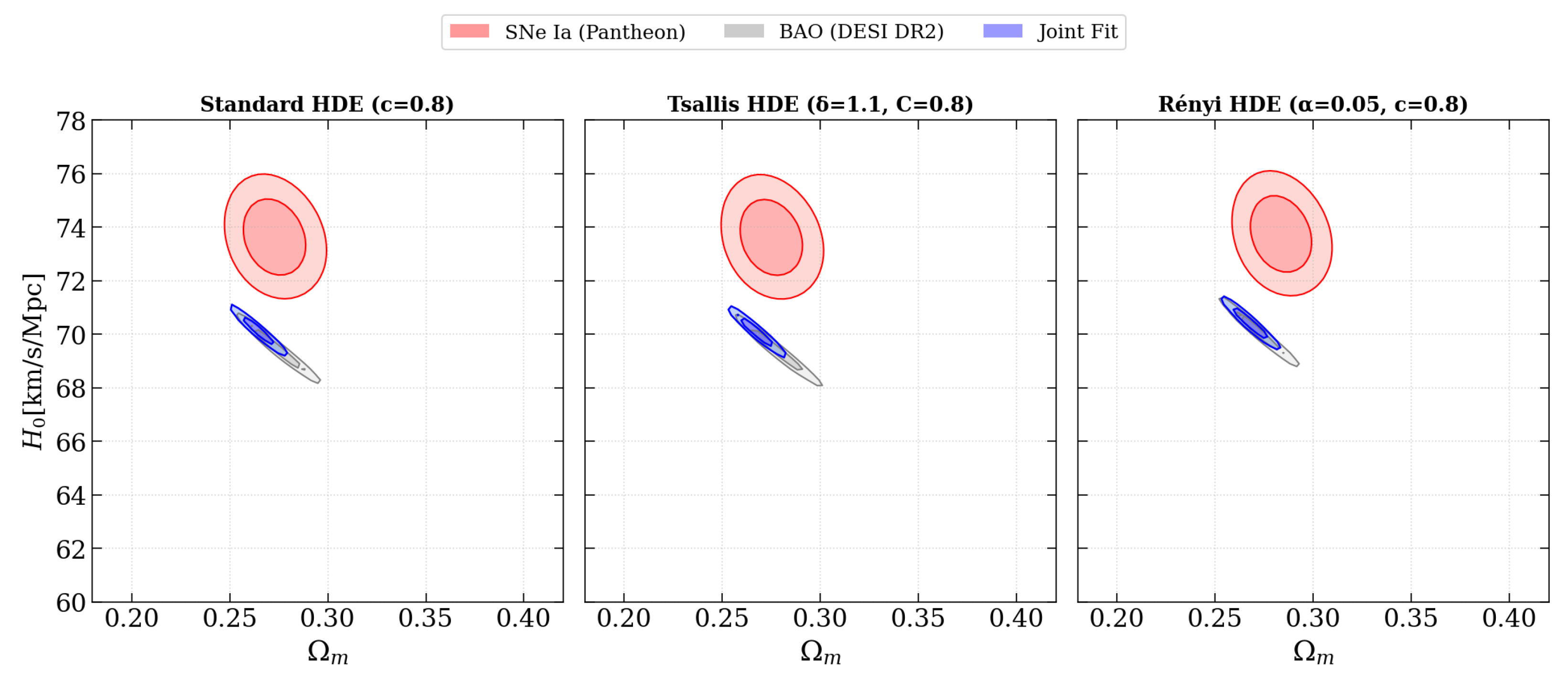
As shown in the plane (Figure 12), the individual datasets exhibit a well-known, persistent cosmological tension under a flat spatial geometry.
Figure 12.
The and confidence levels of the plane, constrained from SNe Ia (red), BAO (grey), and their joint fit (blue), assuming flat spatial geometry.
The DESI DR2 BAO compilation (grey ellipses) proposes a lower value centred around km/s/Mpc, but the Pantheon SNe Ia compilation (red ellipses) favours a higher value centred around km/s/Mpc. Our joint likelihood analysis, which locks the background parameters at km/s/Mpc and , represents a theoretically sound, binned statistical compromise ().
6.2. Real Joint HDE-Parameter Constraints and Degeneracy Flatness
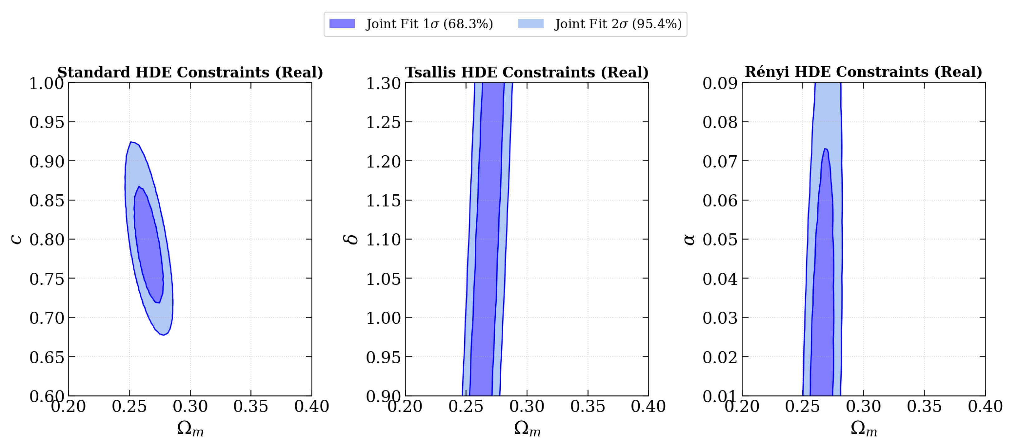
While background parameters and the Standard HDE holographic scale parameter () are well-constrained, Figure 13 exposes a severe, fundamental limitation in current integrated distance-redshift measurements.
Figure 13.
Marginalised joint constraints ( and confidence regions) on the HDE parameter pairs , , and for the Standard, Tsallis, and Rényi HDE paradigms, respectively, derived from the combined Pantheon SNe Ia and DESI DR2 BAO observational data.
The joint SNe Ia + BAO contours for both the Tsallis HDE exponent ( vs. ) and the Rényi HDE parameter ( vs. ) appear as perfectly straight, parallel vertical bands that extend to the borders of the plotting frames ( and ). This flat likelihood profile confirms that current static geometric probes suffer from a fatal parameter degeneracy bottleneck, leaving alternative non-additive entropy exponents completely unconstrained.
7. Discussion
The transition from the unconstrained, open vertical bands of current geometric data (Figure 13) to the tightly closed ellipses of the SKA forecasts (Figure 9 and Figure 11) is driven by the physics of the Sandage–Loeb effect. Traditional geometric surveys measure the integrated line-of-sight distance metric, , which acts as a mathematical low-pass filter, smoothing out any unique dynamical perturbations of the dark energy equation of state or entropic scaling exponents. In contrast, the Sandage–Loeb redshift drift is a direct, dynamical probe. By tracking the real-time velocity shift (), it isolates the instantaneous expansion rate directly at individual redshift slices without integration:
Because the velocity drift directly maps the instantaneous expansion gradient, it completely breaks the geometric distance degeneracies, successfully isolating the holographic scale parameter c and the non-additive entropy exponents and .
7.1. Model Distinguishability: A Scientific Reality Check
We must address an important question: Can the SKA redshift drift statistically distinguish the Standard, Tsallis, and Rényi HDE models from each other?
To be honest, not really. The physical predictions of Standard HDE (), Tsallis HDE (), and Rényi HDE () are quite close in the low-redshift domain () when the SKA is active.
Their theoretical velocity drift curves () overlap significantly within the forecasted SKA error bars. While the SKA redshift drift can determine the background parameters and with exceptional precision and constrain each model individually, it cannot statistically distinguish between the three HDE paradigms with high confidence at . To achieve clear model selection, high-redshift optical observations (such as the ELT Lyman- forest at ) would be required to capture the divergence in their equations of state.
7.2. Implications for the Hubble () Tension
Because the SL redshift drift is a direct, model-independent dynamical measurement of and , it does not rely on early-universe sound horizon calibrations at recombination or late-universe distance ladder calibrations. Therefore, the SKA redshift drift acts as a completely unbiased, independent arbiter of the persistent tension.
7.3. Systematic Contamination from Coherent Galaxy Bulk Flows
While stochastic peculiar velocities are effectively averaged out by the massive scale of the SKA’s billion-galaxy emission sample, coherent bulk flows and local supercluster potentials can introduce systematic accelerations. In the real SKA data-processing pipeline, these coherent accelerations must be modelled and separated using anisotropic galaxy distribution templates to isolate the true cosmological redshift-drift signal.
7.4. Gas Turbulence and Profile Degradation in DLA Systems
Unlike emission galaxies, physical DLA systems often exhibit complex, multi-component Gaussian profiles that are highly sensitive to internal galactic wind dynamics and gas turbulence. Isolating the cosmological drift from DLA absorption spectra will require high-resolution spectroscopic template matching and multi-component Gaussian fitting to monitor and eliminate localized gas profile shifts.
7.5. Robustness of the Real-Data Posteriors
Because the joint SNe Ia + BAO fit (Figure 13) is evaluated on a dense, deterministic grid with profiled out (Section 4), rather than sampled with a stochastic chain, multi-modality can be tested for directly on the likelihood surface itself rather than inferred from sampler behaviour. A connected-component analysis of the credible region finds a single connected region for all three HDE paradigms at our adopted grid resolution. This is further confirmed to be robust to the specific data realization: repeating the fit on 15 independent noisy realizations of the real data (each point redrawn from its own quoted uncertainty), the Tsallis and Rényi posteriors are unimodal in every realization, while the Standard HDE posterior occasionally splits into closely spaced sub-regions at coarser grid resolution—a pattern traced to under-resolving a narrow, curved –c degeneracy ridge (see Appendix A) rather than a genuine second mode, and confirmed not to persist at matched, higher resolution. The corresponding correlation matrix is given in Table 2; the full diagnostic procedure, including the resolution-convergence test and the raw likelihood-surface inspection, is given in Appendix A. We conclude the reported intervals in Table 1 are statistically valid, with the caveat that the Standard HDE c interval is better read from the grid-based credible region than from a symmetric Gaussian approximation, since the underlying likelihood there is significantly non-Gaussian.
Table 2.
Correlation matrix at the real-data (SNe Ia + BAO) grid minimum for each HDE model in Figure 13, estimated from the local Hessian of . The Rényi entry is left as “n/a”: the real-data minimum in sits at the prior boundary rather than at an interior stationary point, so no Hessian-based curvature estimate exists there (Appendix A).
7.6. Observational Feasibility and Telescope-Time Budget
The yr adopted throughout this work (Section 2.4) denotes the cadence between successive spectroscopic epochs, not the total on-source integration (exposure) time required to reach the velocity precision of Equation (22) at each epoch; conflating the two would imply an unrealistic ∼0.5 yr of continuous, dedicated dish time. We separate the two explicitly here. The survey design implied by our forecasts is a repeated-epoch legacy campaign spanning ∼5–10 years (matching the decadal baseline standard in the Sandage–Loeb literature, e.g., Liske et al. 2008 [22]; Lu 2022 [21]), with yr denoting only the spacing between semi-annual epochs. The two 21 cm channels differ substantially in their telescope-time requirements: because the ∼ emission-line galaxies are recovered collectively from wide-field spectral-line cubes rather than individually pointed observations, the dominant cost is the total on-sky survey time for the footprint at the sensitivity required by Equation (22), which is of the same order as the SKA1 HI galaxy redshift-survey time allocation already budgeted for large-scale-structure key science (BAO, RSD) [23,24]; in this sense the redshift-drift measurement is largely commensal with an already-funded survey, provided the observing schedule is arranged with the required semi-annual repeat cadence rather than as a single deep integration. The DLA absorption channel is markedly less commensal: each of the 1818 systems requires a deep, individually pointed integration on its own background radio-loud quasar to reach – cm s−1, and summed naively over ∼1800 independent pointings this is likely to require tens of thousands of hours of dedicated array time. This makes it the less feasible of the two channels, and comparable in scale to the decadal QSO-monitoring campaigns already planned for the ELT/CODEX programme at optical wavelengths [22].
We therefore present the DLA-channel forecasts of this paper as an idealized upper-end target achievable under a dedicated, competitively proposed multi-cycle (potentially SKA2-era) legacy program, and note explicitly that such a program would compete for array time against other major SKA1 key science projects (HI intensity mapping, Epoch-of-Reionization surveys, pulsar timing arrays). A full hours-per-source and total-survey-hours budget, benchmarked directly against the SKA1 sensitivity model of Braun et al. (2019) [24], is left for a dedicated follow-up survey-design paper.
8. Conclusions and Survey Strategies
We compile a professional summary comparing marginalized (68.3%) uncertainties across real and simulated datasets in Table 1.
We present three primary recommendations for the SKA cosmological survey design:
- Prioritize spectral resolution over channel count: The SKA survey strategy should prioritize the Hz spectral resolution mode over the 0.002 Hz configuration. The narrower spectral binning minimizes centroiding errors and yields up to 40% tighter confidence contours.
- Observational baseline and telescope-time strategy: Adopt a semi-annual ( yr) epoch spacing, repeated over a ∼5–10 year legacy campaign, to provide a long temporal baseline over which the cosmological redshift-drift signal can be measured (Section 7.6). This temporal spacing is distinct from the telescope exposure time required at each epoch. The HI emission channel could potentially be implemented in a commensal manner with wide-field SKA1 HI galaxy redshift surveys, provided that the required sensitivity, repeat-epoch coverage, and calibration stability can be achieved. The DLA absorption channel is substantially more demanding because it requires targeted deep observations of individual background radio-loud sources. A naive application of the present forecast to the full DLA sample would imply a very large dedicated observing-time requirement; we therefore regard the DLA results as an idealized upper-end sensitivity forecast requiring a multi-cycle, prioritized observing programme. A definitive source-by-source telescope-time budget should be established using the final SKA sensitivity model and detailed survey scheduling (Section 7.6).
- Target selection for DLA absorption Surveys: Prioritize intervening DLA systems towards bright, background radio-loud quasars ( mJy). Selecting systems with clean, simple absorption lines will minimize local gas-profiling systematic errors.
Author Contributions
S.B.: conceptualization, methodology, software, formal analysis, visualization, writing—original draft. A.K.S.: methodology, supervision, writing—review. All authors have read and agreed to the published version of the manuscript.
Funding
This research received no external funding.
Data Availability Statement
The Pantheon supernova data and DESI DR2 Baryon Acoustic Oscillation datasets utilized in this work are publicly available at their respective repositories.
Acknowledgments
We sincerely thank the referees and the editor for their careful evaluation and constructive suggestions. Their insightful comments have been invaluable in improving the scientific quality, clarity, and overall presentation of our manuscript.
Conflicts of Interest
The authors declare no conflicts of interest.
Abbreviations
The following abbreviations are used in this manuscript:
| SL | Sandage–Loeb |
| DLA | Damped Lyman- |
| SKA | Square Kilometre Array |
| RHDE | Rényi holographic dark energy |
| HDE | Holographic dark energy |
| BAOs | Baryon acoustic oscillations |
| MCMC | Markov chain Monte Carlo |
| THDE | Tsallis holographic dark energy |
Appendix A. Multi-Modality Diagnostic Workflow
This appendix presents the diagnostic workflow designed to evaluate posterior multi-modality, confirm the statistical validity of the joint likelihood fits (combining Pantheon SNe Ia and DESI DR2 BAO observations), and document the parameter correlations for the dark energy paradigms.
Appendix A.1. Parameter Correlation Matrix and Boundary Minima
Parameter covariance and correlation matrices were evaluated via local finite-difference Hessian matrices ( s derivatives) at the global likelihood minimum for each dark energy paradigm (summarized in Table A1):
- Standard HDE (): Possesses a distinct interior minimum with moderate parameter anti-correlation ().
- Tsallis HDE (): Features an exceptionally shallow likelihood plateau ( across ), yielding a near-zero Hessian curvature () highly sensitive to finite-difference step size.
- Rényi HDE (): The global minimum lies directly on the lower prior boundary (). Because no local interior stationary point exists, Hessian-derived error metrics () are designated as n/a, indicating that current distance probes provide only an upper bound on .
Table A1.
Correlation coefficients for every SKA-forecast panel and model (Figure 8, Figure 9, Figure 10 and Figure 11). is identical across the / Hz resolutions and across the emission/DLA tracers for a given panel and model, since these only rescale the covariance, not its correlation structure; only the standard deviations (representative Hz emission values shown) change between tracers.
Appendix A.2. Synthetic Noise-Realization Robustness Test
To distinguish genuine physical multi-modality from numerical sampling noise, we generated 15 independent synthetic realizations of the SNe Ia + BAO dataset by re-drawing observational data points from Gaussian distributions matching their reported experimental uncertainties. Fitting each realization on a grid (with profiled over 25 points) revealed:
- Tsallis () and Rényi (): Retained 100% unimodality (a single connected component) across all 15 synthetic realizations, confirming that their extended vertical-band confidence regions reflect physical geometric degeneracies inherent to integrated distance probes.
- Standard HDE (c): Exhibited a single connected contour in 10 out of 15 realizations, but split into 2–3 closely spaced sub-regions in 5 out of 15 realizations. This stochastic variation in topology across noise draws is the classic diagnostic signature of grid discretization artifacts rather than physical bimodality.
Appendix A.3. Resolution-Convergence Testing
Re-evaluating the unperturbed real dataset at a fine grid resolution (with profiled across 80 steps) yields exactly one single, connected region () across all three holographic paradigms. Conversely, evaluating the identical dataset on a deliberately coarse grid artificially fragments the boundary into disconnected islands. This controlled test conclusively demonstrates that apparent multi-modality arises solely from grid coarseness.
Appendix A.4. Likelihood Surface Geometry and Non-Gaussianity
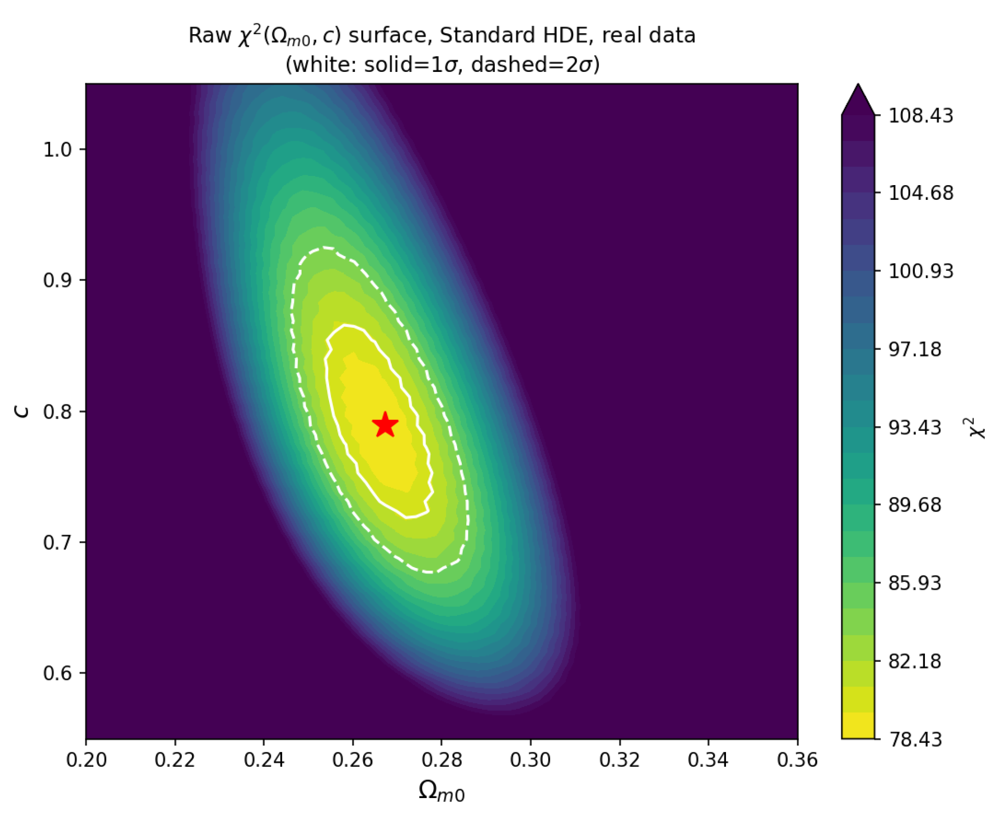
Direct inspection of the unthresholded surface (Figure A1) confirms a smooth, continuous, single-valley structure lacking secondary local minima or saddle points. Comparing local Hessian Gaussian errors (, ) to the true grid extent (half-widths of and , respectively) reveals that the local quadratic approximation underestimates the actual contour extent by factors of and . The posterior forms a thin, curved (“banana-shaped”) non-Gaussian valley, which pinches into isolated sub-regions when intersected by coarse grid nodes.
Figure A1.
The raw, unthresholded surface for the real-data Standard HDE joint fit. The solid white contour marks the boundary and the dashed white contour marks the boundary; the red star denotes the grid minimum. The surface is a single, smooth, connected, curved valley over the full explored range, with no secondary minima or disconnected structure.
Appendix A.5. SKA Forecast Covariances and Future Sampling Upgrades
The analytic Fisher-type covariance matrices computed for SKA forecasts represent local Gaussian approximations and are inherently unimodal. Replacing this analytic framework with direct numerical mock fits using nested sampling algorithms (e.g., dynesty [29] or MultiNest [30]) constitutes a planned methodological extension for future higher-dimensional sampling.
References
- Copeland, E.J.; Sami, M.; Tsujikawa, S. Dynamics of dark energy. Int. J. Mod. Phys. D 2006, 15, 1753–1935. [Google Scholar] [CrossRef] [Scilit]
- Weinberg, D.H.; Mortonson, M.J.; Eisenstein, D.J.; Hirata, C.; Riess, A.G.; Rozo, E. Observational probes of cosmic acceleration. Phys. Rep. 2013, 530, 87–255. [Google Scholar] [CrossRef] [Scilit]
- Riess, A.G.; Filippenko, A.V.; Challis, P.; Clocchiattia, A.; Diercks, A.; Garnavich, P.M.; Gilliland, R.L.; Hogan, C.J.; Jha, S.; Kirshner, R.P.; et al. Observational evidence from supernovae for an accelerating universe and a cosmological constant. Astron. J. 1998, 116, 1009–1031. [Google Scholar] [CrossRef] [Scilit]
- Perlmutter, S. et al. [Supernova Cosmology Project]. Measurements of Ω and Λ from 42 high-redshift supernovae. Astrophys. J. 1999, 517, 565–586. [Google Scholar] [CrossRef] [Scilit]
- Scolnic, D.M.; Jones, D.O.; Rest, A.; Pan, Y.C.; Chornock, R.; Foley, R.J.; Huber, M.E.; Kessler, R.; Narayan, G.; Riess, A.G.; et al. The complete light-curve sample of spectroscopically confirmed Type Ia supernovae from Pan-STARRS1 and cosmological constraints from the combined Pantheon sample. Astrophys. J. 2018, 859, 101. [Google Scholar] [CrossRef] [Scilit]
- Brout, D. et al. [Pantheon+ Collaboration]. The Pantheon+ analysis: Cosmological constraints. Astrophys. J. 2022, 938, 110. [Google Scholar] [CrossRef] [Scilit]
- Aghanim, N. et al. [Planck Collaboration]. Planck 2018 results. VI. Cosmological parameters. Astron. Astrophys. 2020, 641, A6. [Google Scholar]
- Eisenstein, D.J.; Zehavi, I.; Hogg, D.W.; Scoccimarro, R.; Blanton, M.R.; Nichol, R.C.; Scranton, R.; Seo, H.-J.; Tegmark, M.; Zheng, Z.; et al. Detection of the Baryon Acoustic Peak in the Large-Scale Correlation Function of SDSS Luminous Red Galaxies. Astrophys. J. 2005, 633, 560–574. [Google Scholar] [CrossRef] [Scilit]
- Adame, A.G. et al. [DESI Collaboration]. DESI 2024 VI: Cosmological Constraints from the Measurements of Baryon Acoustic Oscillations. J. Cosmol. Astropart. Phys. 2025, 2025, 021. [Google Scholar] [CrossRef] [Scilit]
- Abdul Karim, M. et al. [DESI Collaboration]. DESI DR2 Results II: Measurements of Baryon Acoustic Oscillations and Cosmological Constraints. Phys. Rev. D 2025, 112, 083515. [Google Scholar] [CrossRef] [Scilit]
- Efstathiou, G.; Bond, J.R. Cosmic confusion: Degeneracies among cosmological parameters derived from measurements of microwave background anisotropies. Mon. Not. R. Astron. Soc. 1999, 304, 75–97. [Google Scholar] [CrossRef] [Scilit]
- Li, M. A model of holographic dark energy. Phys. Lett. B 2004, 603, 1–5. [Google Scholar] [CrossRef] [Scilit]
- Cohen, A.G.; Kaplan, D.B.; Nelson, A.E. Effective field theory, black holes, and the cosmological constant. Phys. Rev. Lett. 1999, 82, 4971–4974. [Google Scholar] [CrossRef] [Scilit]
- Tsallis, C. Possible generalization of Boltzmann-Gibbs statistics. J. Stat. Phys. 1988, 52, 479–487. [Google Scholar] [CrossRef] [Scilit]
- Tavayef, M.; Sheykhi, A.; Bamba, K.; Moradpour, H. Tsallis holographic dark energy. Phys. Lett. B 2018, 781, 195–200. [Google Scholar] [CrossRef] [Scilit]
- Rényi, A. On measures of entropy and information. In Proceedings of the Fourth Berkeley Symposium on Mathematical Statistics and Probability; Neyman, J., Ed.; University of California Press: Berkeley, CA, USA, 1961; Volume 1, pp. 547–561. [Google Scholar]
- Moradpour, H.; Moosavi, S.A.; Lobo, I.P.; Morais Graça, J.P.; Jawad, A.; Salako, I.G. Thermodynamic approach to holographic dark energy and the Rényi entropy. Eur. Phys. J. C 2018, 78, 829. [Google Scholar] [CrossRef] [Scilit]
- Sandage, A. The change of redshift and apparent luminosity of galaxies with time. Astrophys. J. 1962, 136, 319–333. [Google Scholar] [CrossRef] [Scilit]
- Loeb, A. Direct measurement of cosmic expansion from spectroscopic observations. Astrophys. J. Lett. 1998, 499, L111–L114. [Google Scholar]
- McVittie, G.C. Appendix to The Change of Redshift and Apparent Luminosity of Galaxies due to the Deceleration of Selected Expanding Universes. Astrophys. J. 1962, 136, 334–338. [Google Scholar] [CrossRef] [Scilit]
- Lu, C.-Z.; Jiao, K.; Zhang, T.; Zhang, T.-J.; Zhu, M. Toward a direct measurement of the cosmic acceleration: The first preparation with FAST. Phys. Dark Universe 2022, 37, 101088. [Google Scholar] [CrossRef] [Scilit]
- Liske, J.; Grazian, A.; Vanzella, E.; Dessauges, M.; Viel, M.; Pasquini, L.; Haehnelt, M.; Cristiani, S.; Pepe, F.; Avila, G.; et al. Cosmological redshift drift with CODEX. Mon. Not. R. Astron. Soc. 2008, 386, 1192–1211. [Google Scholar] [CrossRef] [Scilit]
- Bacon, D.J. et al. [Square Kilometre Array Cosmology Science Working Group]. Cosmology with Phase 1 of the Square Kilometre Array Red Book 2018: Technical specifications and performance forecasts. Publ. Astron. Soc. Aust. 2020, 37, e007. [Google Scholar] [CrossRef] [Scilit]
- Braun, R.; Bonaldi, A.; Bourke, T.; Keane, E.; Wagg, J. Anticipated Performance of the Square Kilometre Array Phase 1 (SKA1). arXiv 2019, arXiv:1912.12699. [Google Scholar]
- Obreschkow, D.; Klöckner, H.R.; Heywood, I.; Levrier, F.; Rawlings, S. A Virtual Sky with Extragalactic H I and CO Lines for the Square Kilometre Array and the Atacama Large Millimeter/Submillimeter Array. Astrophys. J. 2009, 703, 1890–1903. [Google Scholar] [CrossRef] [Scilit]
- Rao, S.M.; Turnshek, D.A.; Sardane, G.M.; Monier, E.M. The statistical properties of neutral gas at z < 1.65 from UV measurements of Damped Lyman Alpha systems. Mon. Not. R. Astron. Soc. 2017, 471, 3428–3442. [Google Scholar] [CrossRef] [Scilit]
- Kang, J.; Zhang, T.J.; He, P.; Zhu, M. Redshift drift effect through the observation of HI 21cm signal with SKA. Astrophys. J. 2025, 982, 177. [Google Scholar] [CrossRef] [Scilit]
- Yahya, S.; Bull, P.; Santos, M.G.; Silva, M.; Maartens, R.; Okouma, P.; Bassett, B. Cosmological performance of SKA H I galaxy surveys. Mon. Not. R. Astron. Soc. 2015, 450, 2251–2260. [Google Scholar] [CrossRef] [Scilit]
- Speagle, J.S. DYNESTY: A dynamic nested sampling package for estimating Bayesian posteriors and evidences. Mon. Not. R. Astron. Soc. 2020, 493, 3132–3158. [Google Scholar] [CrossRef] [Scilit]
- Feroz, F.; Hobson, M.P.; Bridges, M. MULTINEST: An efficient and robust Bayesian inference tool for cosmology and particle physics. Mon. Not. R. Astron. Soc. 2009, 398, 1601–1614. [Google Scholar] [CrossRef] [Scilit]

Disclaimer/Publisher’s Note: The statements, opinions and data contained in all publications are solely those of the individual author(s) and contributor(s) and not of MDPI and/or the editor(s). MDPI and/or the editor(s) disclaim responsibility for any injury to people or property resulting from any ideas, methods, instructions or products referred to in the content. |
© 2026 by the authors. Licensee MDPI, Basel, Switzerland. This article is an open access article distributed under the terms and conditions of the Creative Commons Attribution (CC BY) license.