Dynamics of Coronal Streamer Deflection Under the Impact of a CME-Driven Shock

Abstract

We present a stereoscopic analysis of coronal streamer deflection induced by a CME-driven shock, utilizing multi-viewpoint coronagraph observations from STEREO-Ahead, STEREO-Behind, and SOHO. Driven by the continuous impact of the shock, the streamer deflection propagates outward, exhibiting distinct morphological variations across the three different lines of sight. Our analysis reveals that speeds derived directly from two-dimensional (2D) images differ significantly from those obtained via three-dimensional (3D) reconstruction. Specifically, the 2D projected speeds measured from STEREO-Ahead, STEREO-Behind, and SOHO are 445, 476, and 336 km s⁻¹, respectively. Furthermore, while 2D measurements suggest a constant propagation speed, the 3D reconstruction reveals a pronounced deceleration of approximately −36 m s⁻². Significant discrepancies are also noted in the deflection amplitude between the 2D and 3D results. Since the propagating streamer deflection effectively traces the shock’s movement, we propose that measuring the deflection speed offers a robust alternative for deriving actual shock velocities in the outer corona, where direct white-light detection remains challenging.

1. Introduction

Magnetohydrodynamics (MHD) waves are ubiquitous in the magnetically dominated solar corona, since they are easy to excite in such an elastic and compressible plasma medium [1,2,3,4,5,6,7]. With the development of observational techniques and many ground-based and space-borne instruments in recent decades, various kinds of wave phenomena have been discovered in the solar atmosphere, for example, large-scale (global) extreme-ultraviolet (EUV) waves [8,9,10], the slow magnetosonic waves in coronal plumes [11,12], quasi-periodic fast-propagating magnetosonic waves [13,14,15,16,17,18,19,20], and sunspot waves [21,22]. Coronal structures such as loops and filaments can exhibit transverse oscillations driven by coronal waves. EUV Moreton waves have been observed to trigger filament oscillations [23,24,25,26,27,28,29,30,31]. In addition to extensive observational studies, many theoretical and simulation endeavors have also been performed in recent decades [32,33,34,35,36,37,38]. These studies have made great progress in our understanding of the physical properties of coronal MHD waves and the corona plasma.

A shock wave is a type of propagating disturbance that propagates faster than the local sound speed in a fluid such as the solar corona. There are two types of shocks, distinguished by their different drivers: piston-driven and CME-driven shocks. In the solar corona, a piston-driven shock can be excited by a sudden pressure pulse such as an impulsive flare, while a CME-driven shock is generated by a fast CME [8]. For CME-driven shocks in the outer corona, [39] observed that a group of raylike features is pushed aside or bent by the laterally expanding CME, and they suggested that the CME-driven shock causes disturbance of the raylike structures. With white-light coronal images taken by the Large Angle Spectrometric Coronagraph (LASCO) [40] onboard the Solar and Heliospheric Observatory (SOHO) [41], Sheeley et al. [42] also reported many shocks propagating ahead of fast CMEs, which can result in kinks in streamers and other raylike features that extend in all directions from the Sun. The streamer kinks decelerate as they propagate outward radially, indicating the deceleration of the shocks. Since CME-driven shocks are faintly visible ahead of CMEs in white-light observations, the response of the aside streamer and raylike structures could be good proxies for detecting shocks in the outer corona [43,44].

Magnetic interaction between solar eruptions and coronal magnetic structures is well-documented in the literature [45,46,47]. The interaction of shocks with streamers has been further studied recently with high-resolution white-light coronagraph images. van der Holst et al. [48] reported the deflection of a streamer caused by a fast CME (say, $v\ge$ 1000 km s⁻¹) that is associated with a type-II radio burst. The authors interpreted the fine structures, such as splitting, of the radio burst as the result of the CME-streamer interaction, and they suggested that the CME-driven shock partially penetrates and then dies away in the denser streamer plasma. Liu et al. [49] also observed the deflection of a streamer caused by a CME-driven shock. They showed that the shock height–time curve determined from the type-II burst is consistent with the shock propagation obtained from the streamer deflection. This confirms the causal relationship between metric type-II burst and CME-driven shock. Moreover, due to the impulsive action of a compressed magnetic field to the leg of the streamer, Eselevich et al. [50] proposed that a blast shock can be excited by the recovery of the deflected streamer. Sometimes, fast CMEs can launch sinusoidal wavelike motions along streamers, and this phenomenon was interpreted as fast kink body waves [51,52,53]. Filippov et al. [54] reported a CME–streamer interaction event, in which the streamer axis deflects impulsively and then returns very slowly to its initial position. This observation does not support the streamer wave interpretation, nor the deformation of a streamer under the action of a propagating shock. They interpreted it as the effect of the magnetic field of a moving magnetic flux rope, which changes the surrounding magnetic field lines. Liu et al. [55] observed the permanent displacement of a streamer structure due to the disruption of a CME, and they suggested the occurrence of magnetic reconnection between the CME and the streamer magnetic fields. In addition, the interaction between streamers and shocks is useful to determine the source region of the type II radio burst associated with CMEs [56]. Therefore, the study of the interaction between shocks and streamers is important for diagnosing the physical properties of CMEs, shocks, and streamers.

As mentioned in the work of Feng et al. [53], the observational view angle is an important factor in the observation of the response of streamers to the impact of CMEs, even though the authors did not provide any evidence on this point. Taking advantage of the three-angle observations taken by Solar Terrestrial Relations Observatory (STEREO) [57] and SOHO, we present the first stereoscopic observational analysis of the deflection characteristics of a streamer resulting from the interaction of a CME-driven shock. This provides a good opportunity for us to study the influence of the observational angle on the streamer deflection and the associated CME-driven shock. As demonstrated in previous STEREO-based reconstructions (e.g., Zuccarello et al. [58], Bi et al. [59], Zhang et al. [60]), multi-viewpoint data are essential to mitigate projection biases inherent in single-line-of-sight coronagraph observations. The present study builds on this foundation by providing a clear, quantitative characterization of such projection effects in the specific scenario of CME-driven shock-streamer interaction. Instruments and observations are briefly introduced in Section 2. Observational results based on the STEREO and SOHO coronagraphs and the Solar Dynamics Observatory (SDO) [61] are described in Section 3. Conclusions and discussions are presented in the last section.

2. Instruments and Observations

The LASCO onboard SOHO is composed of two white-light coronagraphs named C2 and C3, whose FOVs are 1.5–6.0 and 3.7–$30.0R_{\odot }$ from the solar center, with a pixel size resolution of 11.4” and 56”, respectively. We only use the C3 observations that have a cadence of 12 min. STEREO has two satellites, and they are ahead of and behind Earth in their orbits, respectively. The Extreme Ultraviolet Imager (EUVI) onboard STEREO provides full-disk observations with four wavelengths including 195 Å, 304 Å, 171 Å, and 284 Å, and the pixel size resolution is of 1.6”. We use the 195 Å and 304 Å images, whose cadences are 5 and 10 min, respectively. Each STEREO satellite has two white-light coronagraphs named COR1 and COR2, which observe the inner (1.4–$4.0R_{\odot }$) and the outer (2.0–$15.0R_{\odot }$) corona, respectively. Only the COR2 images are used in this paper, whose pixel size resolution is 14.7”, and the cadence is 15 min. For convenience, we refer to the instruments onboard STEREO Ahead and Behind as EUVI-A, EUVI-B, COR2-A, and COR2-B. The Atmospheric Imaging Assembly [62] onboard SDO takes full-disk images of the sun with seven EUV and three ultraviolet wavelengths. The AIA 304 Å and 193 Å images are used, whose pixel size resolution and cadence are 0.6” and 12 s, respectively.

3. Observational Results

On 1 May 2013, a prominence erupted from the back side of the Sun with respect to Earth near the east limb, producing a partial halo CME detected jointly by the LASCO C2 and C3 detectors aboard SOHO. The CME was first observed in LASCO C2 at 03:12:08 UT and in LASCO C3 at 03:24 UT, with key parameters retrieved from the CDAW catalog 1. Its first onset at $1R_{\odot }$ was recorded at 02:15:32 UT and a second onset at $1R_{\odot }$ was noted at 02:34:16 UT. The on disk eruption onset was captured at 02:35 UT by EUVI-B, providing comprehensive time coordinates to facilitate event identification in the catalog and the tracking of its initiation and propagation. The CDAW catalog is a dedicated resource for LASCO observations, compiling data from both C2 and C3 detectors. According to this catalog, the CME’s linear speed is 762 km s⁻¹. The acceleration value of −21.7 m s⁻² is derived from a second-order polynomial fit to the continuous height–time sequence of the CME’s leading edge, with observational points spanning $4.06R_{\odot }$ to $22.13R_{\odot }$, as recorded by LASCO C2 and C3. The CME’s first onset at $1R_{\odot }$ is noted at 02:15:32 UT and a second onset at $1R_{\odot }$ at 02:34:16 UT. The position angle of approximately 42° corresponds to the FEAT_PA parameter in the catalog, with its zero point defined as solar north following standard solar observational coordinates.

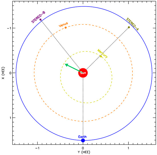
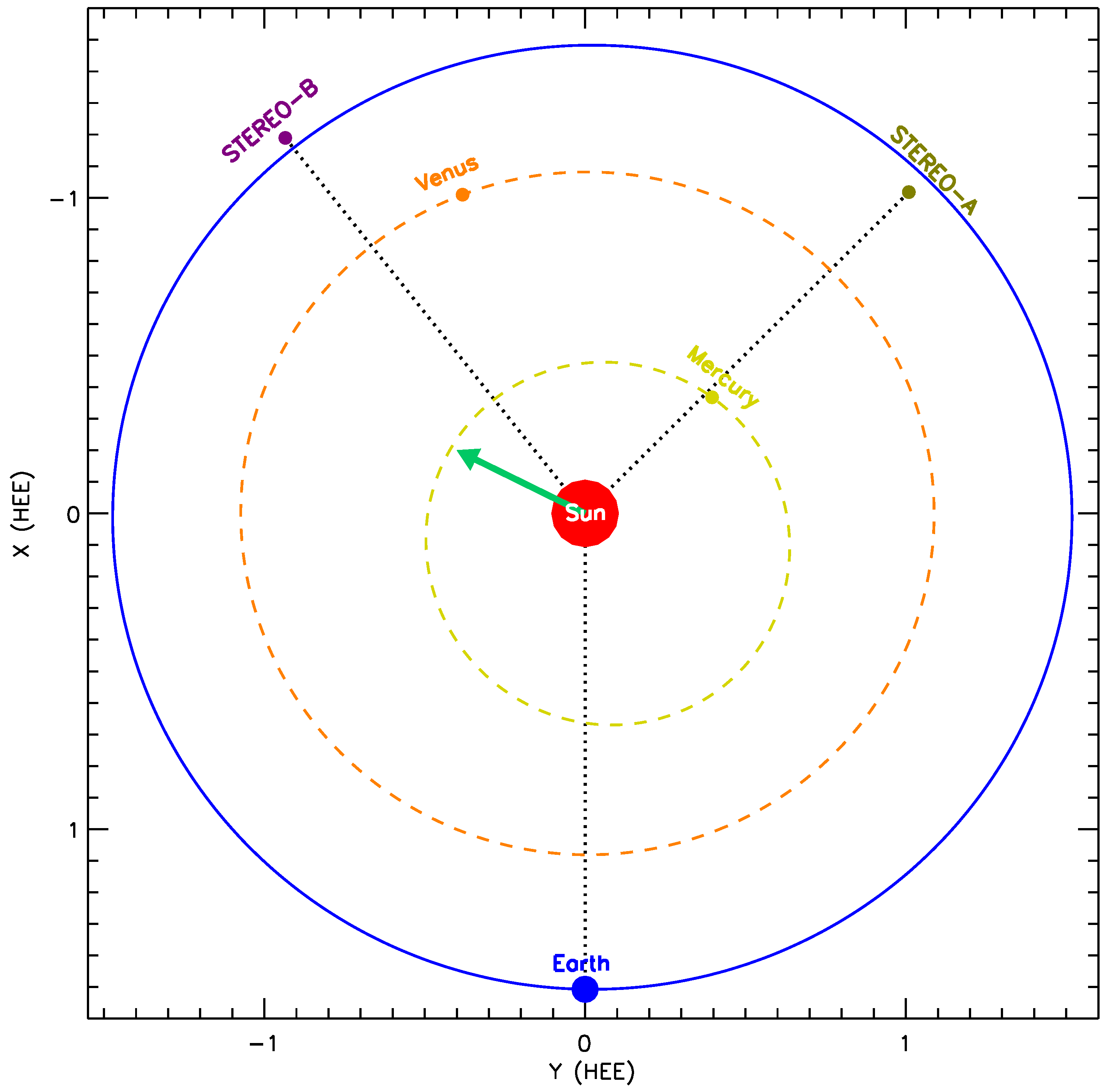
From the other two viewing angles, the twin STEREO satellites also observed this prominence eruption. Figure 1 shows the different view angles and positions of STEREO Ahead and STEREO Behind relative to Earth (i.e., the positions of SDO and SOHO), and their relationship between Mercury, Venus, and the Sun (at 03:00 UT). Earth is defined as the zero point for measuring separation angles, with angles calculated counterclockwise in the orbital plane. The separation angle of STEREO Ahead from Earth is 135°, and that of STEREO Behind is −141°. The negative value indicates a clockwise measurement, which is equivalent to 219° in the counterclockwise direction. This configuration results in an actual separation angle of 83° between STEREO Ahead and STEREO Behind, consistent with their orbital geometry. Figure 1 marks the true eruption direction of the prominence with a green arrow. This direction is determined via a three-dimensional reconstruction of the CME using the triangulation procedure implemented in the scc_measure.pro code of the SolarSoftWare (SSW) package. The reconstruction integrates simultaneous paired coronagraph images from COR2-A and COR2-B and extracts the CME’s leading edge features to resolve spatial ambiguities, and the derived direction is a de-projected radial direction relative to the Sun that eliminates line-of-sight projection biases. Since this eruption occurred on the back side of the Sun, SDO and SOHO can not observe the source region. Fortunately, STEREO Behind can observe it from another view angle. The source region of the eruption was on the northwest of the solar disk, as seen from STEREO Behind.

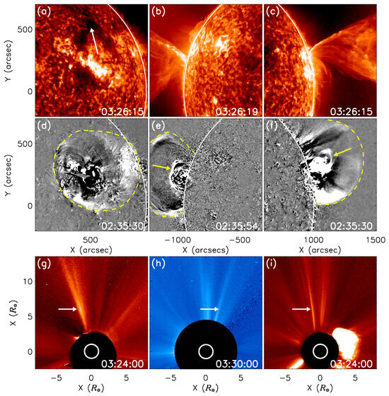
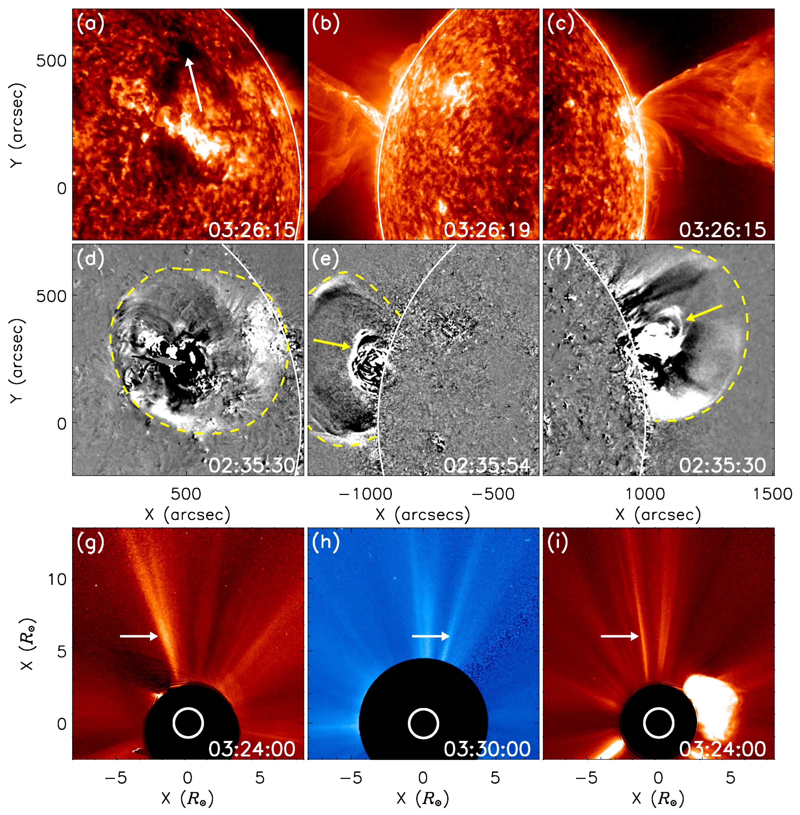
The eruption of the prominence and the associated shock close to the disk limb are shown in the top and middle rows of Figure 2, using 304 Å direct images and 195 Å (193 Å) running difference images. One can see that the erupting prominence is over the east (west) limb in AIA (EUVI-A) 304 Å images (see Figure 2b,c), whereas it is visible on the disk as an erupting filament in EUVI-B 304 Å images (see Figure 2a). In EUVI 195 Å and AIA 193 Å running difference images, an obvious shock can be observed preceding the erupting prominence or filament on the disk. As shown in the middle row of Figure 2, the front of the shock is highlighted with a dashed yellow curve, while the erupting prominence is indicated by a yellow arrow. During the initial stage of the prominence eruption, a streamer remained steady at the solar north in the coronagraph observations. The separation angle between the streamer and the eruption direction of the prominence is larger than 90° (see Figure 2h,i). This angular separation is calculated relative to the true eruption direction of the prominence, indicated by the green arrow in Figure 1. It is measured on the plane of sky corresponding to the observational perspective of each coronagraph in Figure 2, quantifying the directional spacing between the streamer’s axis and the prominence’s eruption path within the two-dimensional observational plane of the coronagraphs. We show the streamer with COR2-A, COR2-B, and LASCO C3 images in the bottom row of Figure 2. As indicated by the horizontal arrows, due to the different view angles, the streamer showed different shapes and positions in different coronagraph images. It should be noted that the radius of coronagraphs’ inner occulting disk is different for LASCO C3 and COR2, at 4.5 and $2.5R_{\odot }$, respectively. At 03:24 UT, the bright CME front had already appeared in the FOV of COR2-A, but COR2-B and LASCO C3 did not detect any signal. This indicates that the source region of the eruption observed from STEREO Ahead is close to the west limb. A faint shock can be observed ahead of the bright CME front in the time-elapsed animations available in the online journal.

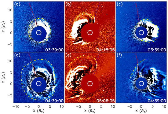
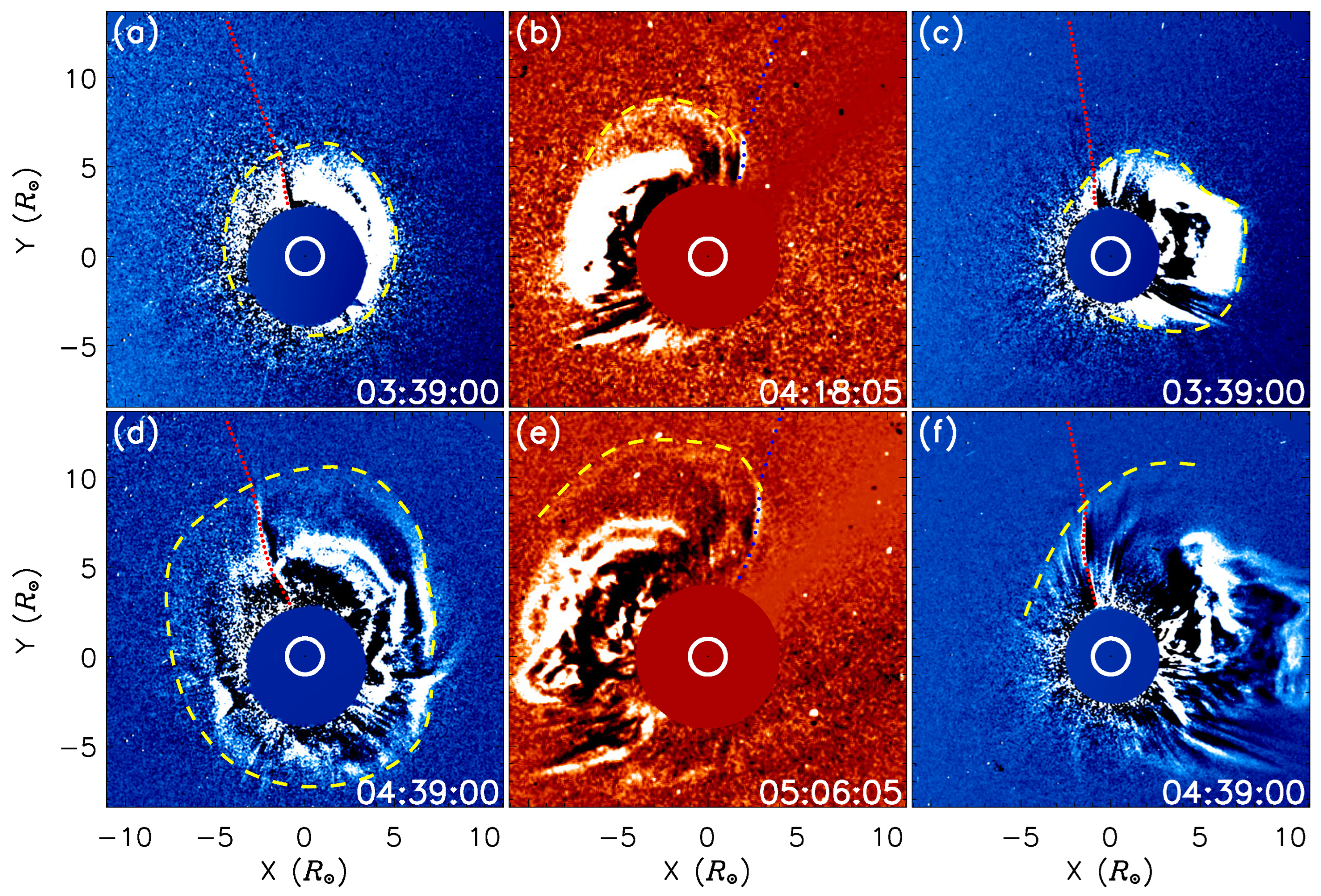
With the high spatial and temporal resolution and the advantage of simultaneous multi-angle observations of the STEREO coronagraphs, we can determine the detailed interaction process between the streamer and the shock that was driven by the CME launched by the prominence eruption. Previous studies [54,55] did not state this point clearly, probably due to the limitations of low-resolution and single-angle observations. For instance, Filippov et al. [54] reported a CME–streamer interaction event where the streamer axis deflected impulsively and then returned slowly to its initial position; they attributed this behavior to the magnetic field of a moving magnetic flux rope altering the surrounding field lines, with no evidence of shock involvement. Similarly, Liu et al. [55] observed the permanent displacement of a streamer following CME disruption, which they interpreted as a result of magnetic reconnection between CME and streamer magnetic fields rather than the impact of a propagating shock. It is noted that the CME is preceded by a faint shock in the low corona, as shown in Figure 2. This shock signature, initially detected in AIA and EUVI images at ∼$1R_{\odot }$ in the plane of sky, is also visible in the coronagraphs (COR2 and LASCO C3) as it propagates outward, extending up to ∼$15R_{\odot }$ (the upper FOV limit of COR2) and ∼$30.0R_{\odot }$ (the upper FOV limit of LASCO C3) in the plane of sky. For each coronagraph observation, we show two moments of the shock–streamer interaction (at the beginning and during the interaction) in Figure 3, using running difference images obtained by subtracting the previous image from the current one. The positions of the streamer and the front of the shock are indicated with dashed curves and dotted lines in the figure, respectively. In COR2-B observations, the CME and the shock span 360°, while in LASCO C3 and COR2-A, they are just observed over the east and west limbs of the Sun, respectively. Due to the higher spatial resolution of the COR2 observations, the shock observed in COR2 images is clearer than that in LASCO C3.

When the shock reached the streamer, the latter immediately deflected to the propagation direction of the shock, and the region of the interaction position between the streamer and the shock became brighter than before in the running difference coronagraph images, especially at 04:39 UT (COR2) and 05:06 UT (LASCO C3). Notably, while the brightness variation is observable in Video S2, the shock front can be more distinctly recognized by referencing the high-definition reference videos from the CDAW catalog 2. These authoritative videos offer a clearer visualization of the CME-driven shock propagation and its dynamic interaction with the coronal streamer, facilitating direct comparison for identifying the shock front. The enhancement of the brightness at the interaction position indicates the movement of the streamer due to the impingement of the shock and the increase in plasma density there. After the interaction, the deflected streamer started to recover due to the magnetic tension, and in the meantime, wavelike motions were observed along the streamer. This is different from the so-called “streamer wave” reported in Chen et al. [51], which shows a sinusoidal wavelike motion along the streamer after the passing of the associated CME. In the present event, the streamer did not show periodic motion after the interaction. Therefore, the wavelike motion along the streamer in the present case is nothing but the deflection of the streamer due to the continuous interaction of the propagating shock. Here, the movement of the streamer deflection reflects the propagation of the shock along the streamer. Since the shock became larger and fainter as it propagated outward, it is hard to measure the wave speed based on the direct coronagraph observations. However, we can obtain the velocity component of the shock along the streamer by measuring the moving speed of the streamer deflection.

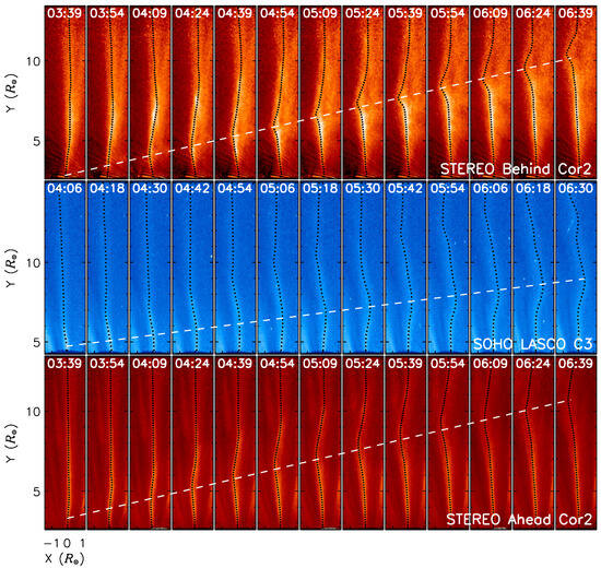
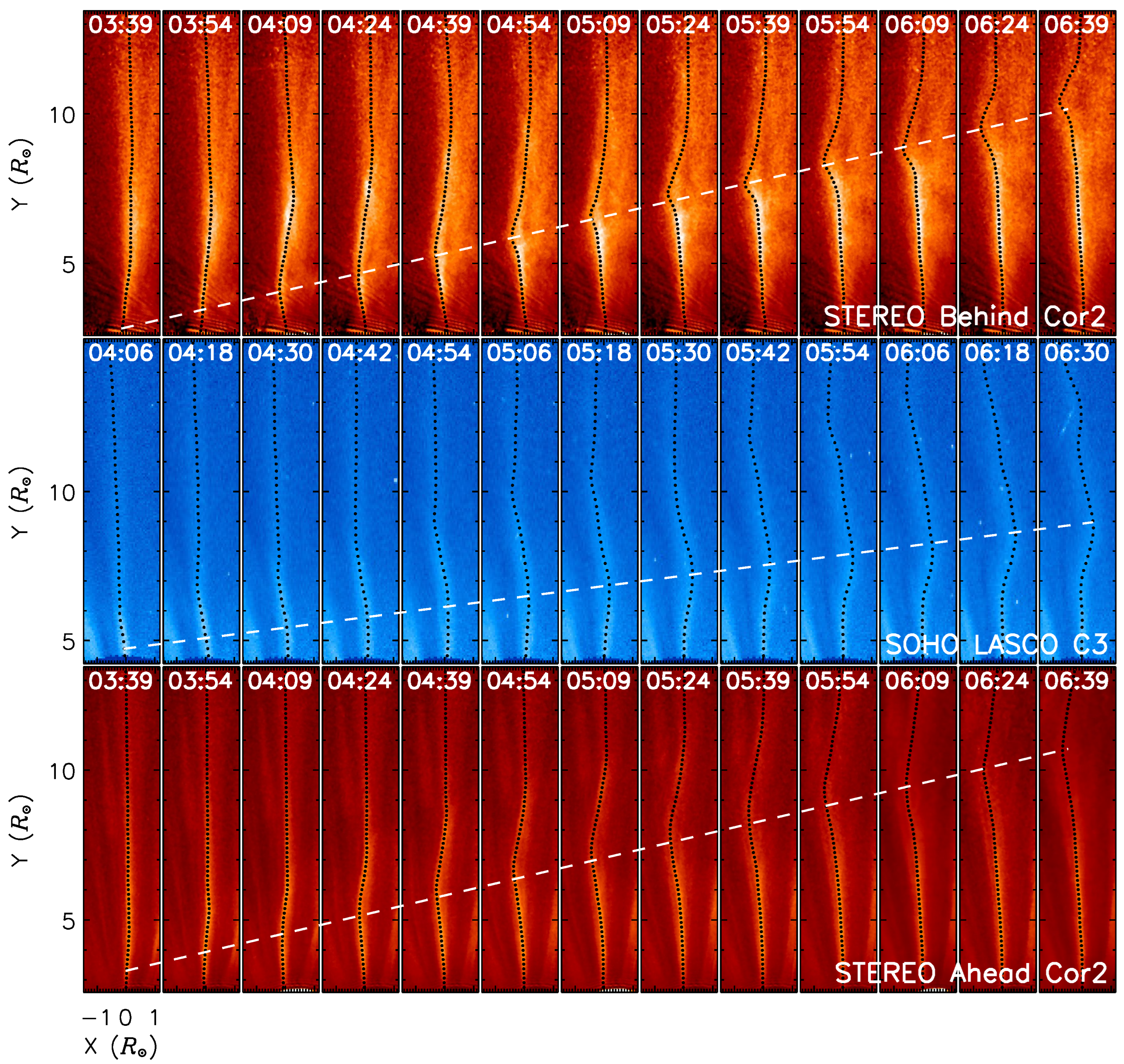
The detailed evolution of the streamer deflection is shown in Figure 4 with white-light observations taken by COR2-B (top row), LASCO C3 (middle row), and COR2-A (bottom row). The axis of the streamer is traced according to the intensity profile perpendicular to the streamer axis every ten pixels. We adopt the position of the maximum value as the center of the axis of the streamer. The traced streamer axis overlaps the corresponding coronagraph image, which shows the kinematics of the streamer deflection more clearly. The streamer deflection amplitude is defined as the maximum perpendicular distance between the deflected streamer axis at the peak of interaction and the initial equilibrium axis before shock impact on the plane of sky. In COR2-B observations, the brightness at the interaction position is enhanced significantly due to the increase in plasma density there. From the center of the deflection, the slope of the bottom part is steeper than the top part, suggesting the interaction between the shock and the streamer is from the above direction with a small angle to the right. In the LASCO C3 view angle, the shock impacted the streamer from the left side, and the deflection of the streamer is smoother than that observed from the COR2-B view angle. In the COR2-A view angle, the shock interacted with the streamer from the right side, and the deflection is in the opposite direction relative to the observation from the LASCO view angle. The center positions of the deflection at different times are connected by a dashed white line in Figure 4, which clearly shows the movement of the deflection along the streamer, and the slope of the lines represents the speed of the deflection structure of the streamer. The moving speed of the deflection structure of the streamer in LASCO C3 observations is obviously slower than that in the COR2 observations.

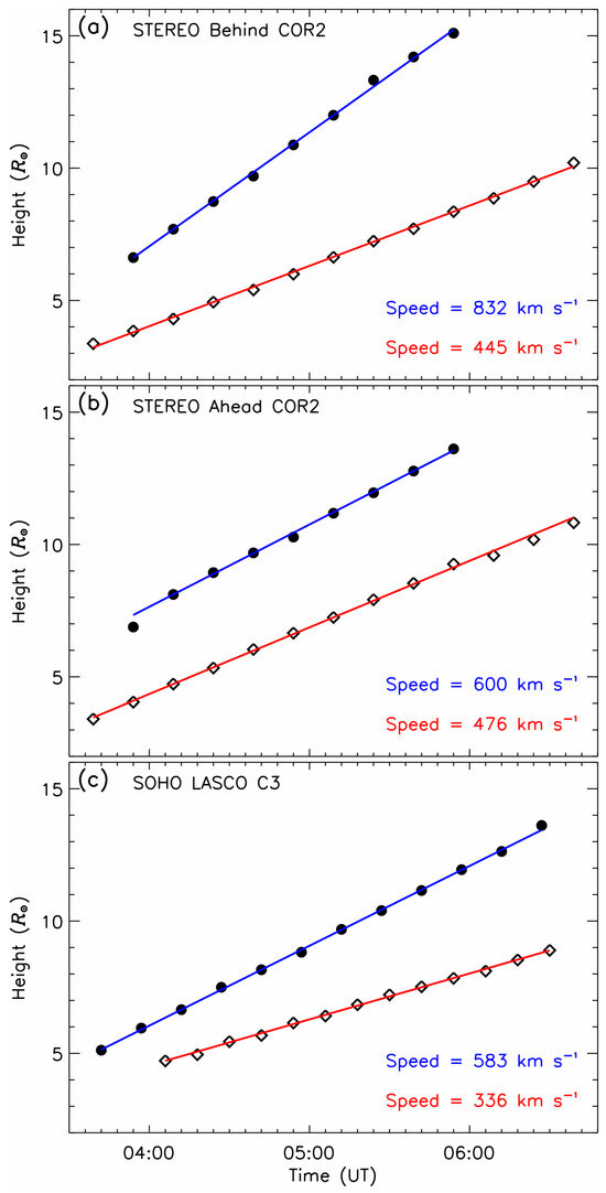
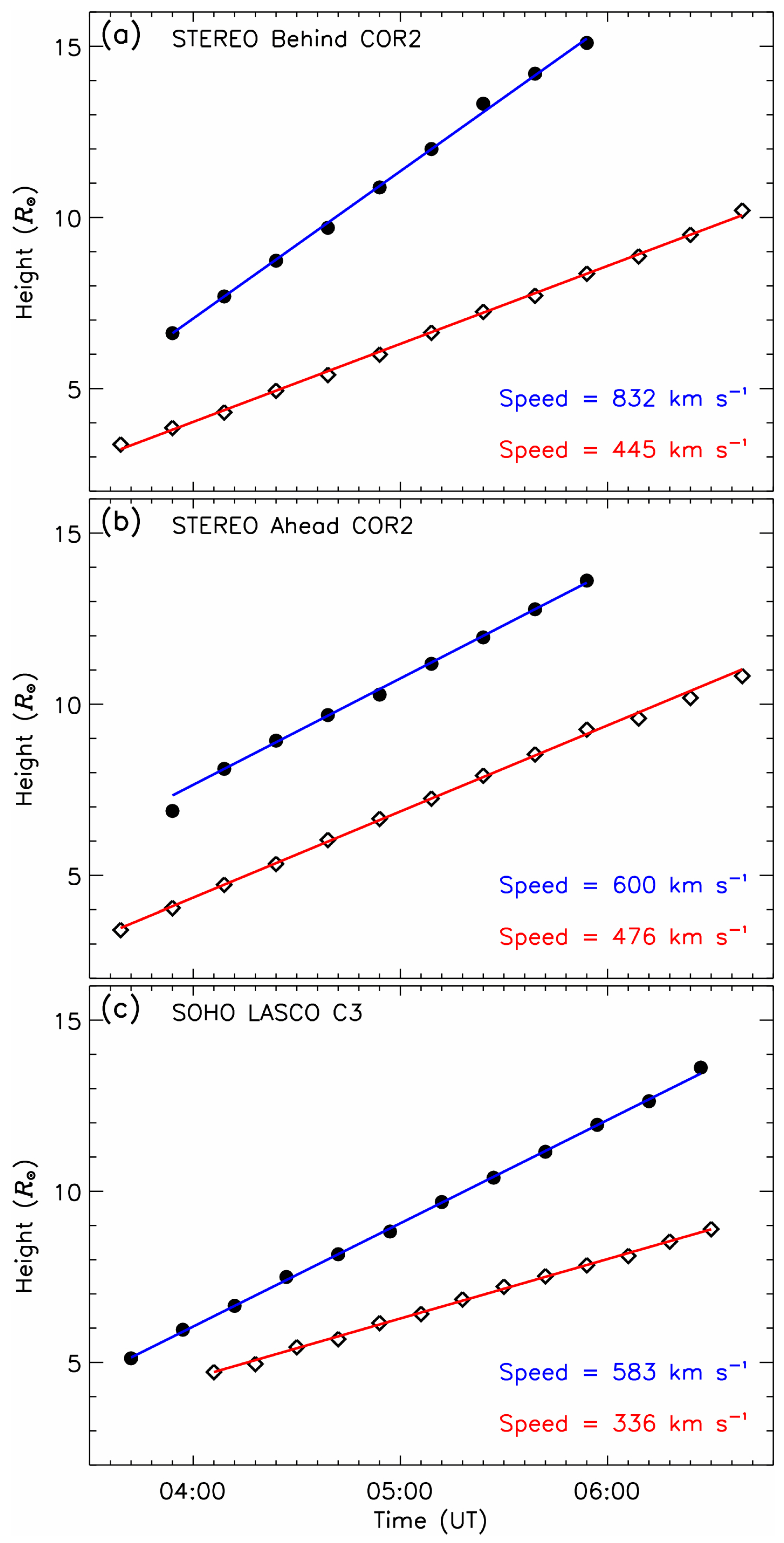
A quantitative analysis of the streamer deflection is shown in Figure 5. By tracing the center position of the streamer deflection, we can obtain the moving speed of the deflection along the streamer and the deflection amplitude relative to the equilibrium position of the streamer. The moving deflection of the streamer represents the propagation speed component of the shock along the streamer direction on the plane of sky. The height–time plots show that the measured height of the center position of the deflection is well fitted using a linear function (red), and the slope yields the velocity component of the shock along the streamer. The results show that the projected speeds measured from COR2-B, COR2-A, and LASCO C3 observations are 445, 476, and 336 km s⁻¹, respectively. While the speeds obtained from COR2-A and COR2-B show little difference, the speed derived from LASCO C3 is slower than that from COR2. This is probably due to the deceleration of the shock and the lower spatial resolution of the LASCO C3 observations. We also measured the shock speeds along the direction perpendicular to the wavefront from different coronagraph observations by tracing consistent and prominent brightening features at the shock front (marked as black dots in Figure 5, corresponding to the yellow dashed shock fronts in Figure 3); the results are 832, 600, and 583 km s⁻¹, respectively. This time, the projected speeds of the shock obtained from the COR2-A and LASCO C3 images are similar, but those derived from COR2-B were very different from the other two coronagraphs. This difference is possibly a result of the projection effect, since a shock driven by a CME often has a dome shape in the low corona [63,64] and the outer corona [65]. One should note that the shock in both COR2-A and LASCO C3 is launched at the solar limb and interacts with the streamer from the side, but it was observed on the disk from the STEREO Behind view angle. In addition, since the wavefront of the shock became more and more faint as it propagated outward, the speed of the shock directly measured from the coronagraph observations should have a bigger error than that derived from the movement of the streamer deflection.

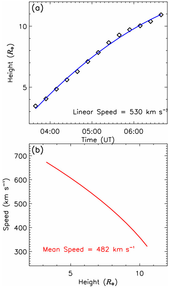
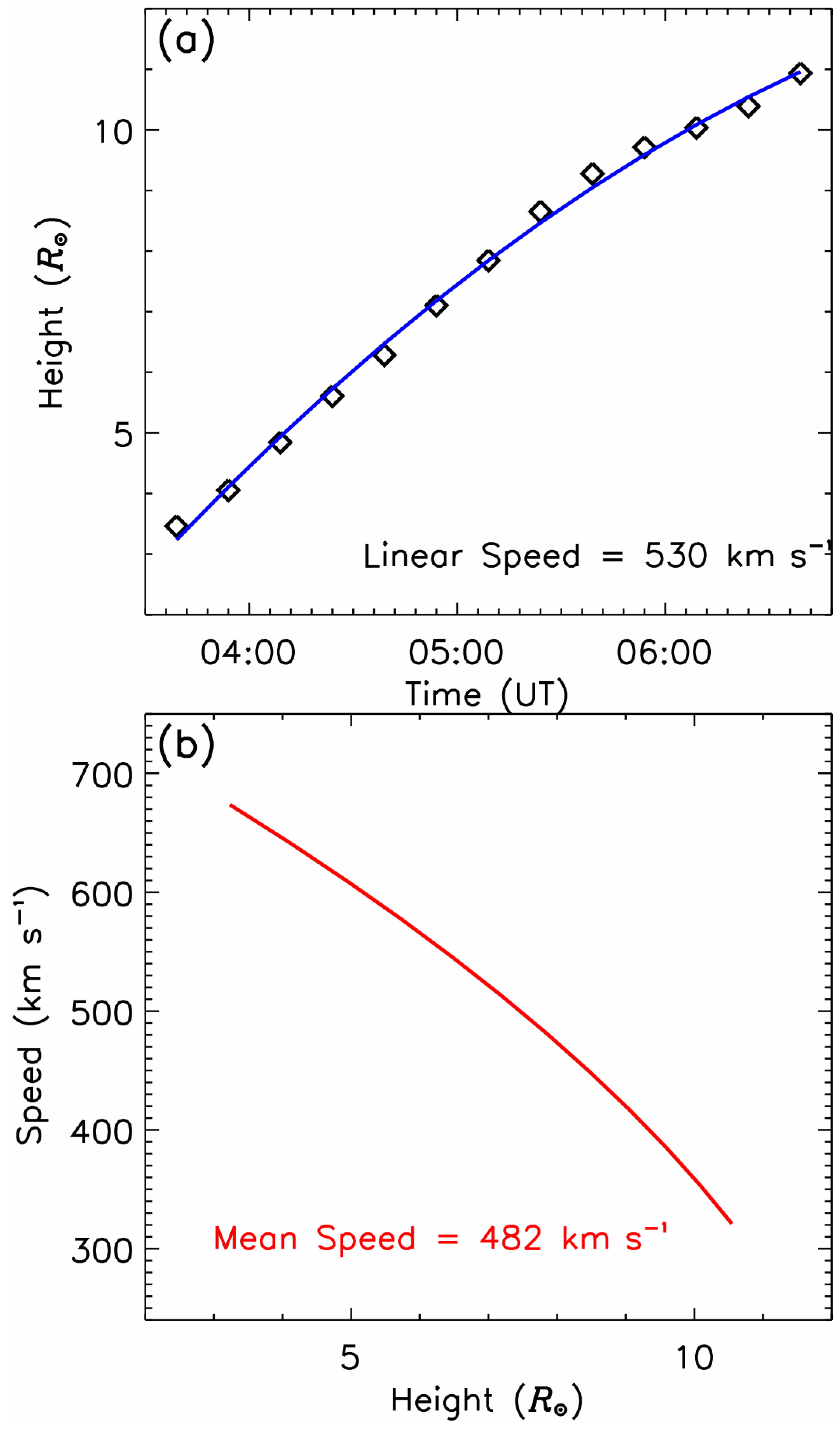
Using the simultaneous paired coronagraph images taken by COR2-A and COR2-B, we further measure the three-dimensional center position of the streamer deflection with a triangulation procedure (scc_measure.pro) available in the SolarSoftWare (SSW) package. This tool outputs not only the 3D position but also the angle of the tracked streamer deflection feature relative to the sky plane for each instrument. The height–time result is shown in the top panel of Figure 6. This shows that a linear fit is no longer suitable for the reconstructed height–time relation of the streamer deflection. Therefore, we use a second-order function (blue curve) to fit the data. This indicates that the movement of the streamer deflection decelerates with the increase in height, and the deceleration is of about −36 m s⁻². This is very different from the results directly measured from the coronagraph observations, where the propagation of the streamer deflection was at a constant speed. We also plot the moving speed of the streamer deflection in the bottom panel in Figure 6, which represents the velocity component of the shock along the streamer. This shows that the speed at $4R_{\odot }$ is about 650 km s⁻¹. When the streamer deflection reached $10R_{\odot }$, the moving speed of the streamer deflection decelerated to 360 km s⁻¹. This suggests the fast deceleration of the shock as it propagates outward. In addition, the amplitude of the streamer deflection is also measured; while the maximum amplitude obtained from the three-dimensional reconstruction is $2.4R_{\odot }$, the results obtained from COR2-B, COR2-A, and LASCO C3 independently are 1.1, 1.6, and $1.4R_{\odot }$, respectively. For 3D triangulation via scc_measure.pro we selected the corresponding axis center points traced from intensity maximum in paired COR2-A and COR2-B images as the consistent features to ensure reliable reconstruction. These features are stable and free of background noise or instrumental artifacts. In addition to the static maximum amplitude, we further analyzed the evolution of deflection amplitude with height using 3D triangulation results ($4R_{\odot }$∼$10R_{\odot }$). The 3D amplitude gradually increases from ∼$1.2R_{\odot }$ at $4R_{\odot }$ to the peak of $2.4R_{\odot }$ at ∼$7R_{\odot }$, then remains stable until $10R_{\odot }$. This dynamic trend is distinct from 2D measurements ($1.1R_{\odot }$–$1.6R_{\odot }$), which only reflect line-of-sight projections and fail to capture the true interaction process. The present results highlight the importance of three-dimensional observations in overcoming projection effects when studying shock and streamer kinematics, consistent with prior stereoscopic studies.

4. Conclusions and Discussions

In this paper, we present the first stereoscopic observations of the deflection characteristics of a streamer caused by a CME-driven shock on 1 May 2013, using high-temporal and high-spatial-resolution observations taken by the space-borne SOHO, SDO, and the twin STEREO satellites from three different view angles. It is found that the streamer deflection is in fact induced by the interaction of the CME-driven shock rather than by the CME directly. The projection speeds of the shock measured from different view angles are 2D projected velocities on the plane of the sky, estimated by tracing prominent brightening features at the CME-driven shock front from COR2-B, COR2-A and LASCO C3 observations via linear fitting to their height–time sequences. The speeds are 832 ± 9 (STEREO Behind), 600 ± 8 (STEREO Ahead) and 583 ± 12 (Earth) km s⁻¹, respectively. These errors are comparable to those of the streamer deflection speeds, confirming the reliability of the velocity measurements derived from the same method.

The streamer deflection showed different shapes in different coronagraph observations (i.e., different view angles). Detailed measurement indicates that the moving speeds of the streamer deflection along the streamer on the plane of sky are 445, 476, and 336 km s⁻¹ based on COR2-B, COR2-A, and LASCO C3 observations, respectively. Since the moving deflection of the streamer is formed due to the continuous pushing of the shock, the speed of the moving deflection of the streamer represents the velocity component of the shock along the direction of the streamer. Since the shock became increasingly fainter as it propagated outward, it is very hard to measure the actual speed of the shock based on the direct coronagraph images. Therefore, measuring the moving speed of the streamer deflection should be an alternative way to obtain the actual speed of the shock.

With single-view-angle observations, one can only measure the two-dimensional projection speed of shocks. Taking advantage of the stereoscopic observations of STEREO, it is possible to derive the three-dimensional kinematics of shocks and other coronal structures, such as streamers [66]. In the present paper, we reconstruct the three-dimensional kinematics of the moving deflection of a streamer resulting from the interaction of a CME-driven shock. The triangulation procedure via scc_measure.pro provides the angle of the tracked feature relative to the sky plane, which enables the de-projection of the sky-plane velocities. High-resolution and multi-angle observational results indicate that the kinematics of the streamer deflection are very different from those obtained with single-view-angle two-dimensional imaging observations. Based on single-view-angle coronagraph images, it is found that the propagation of the deflection of the streamer and the shock remains at a constant speed as they propagate outward. However, the three-dimensional reconstruction results indicate that the moving speed of the streamer deflection decreases with the increase in height and with a deceleration of about −36 m s⁻². The speed derived from secondary polynomial fitting indicates that the moving speed of the streamer deflection at $4R_{\odot }$ is about 650 km s⁻¹, and at $10R_{\odot }$, its speed decelerated to 360 km s⁻¹. This suggests that the shock decelerated faster with the increase in height. As discussed above, the kinematics of the deflection actually reflect the properties of the shock. Therefore, the deceleration of the streamer deflection represents the slowing down of the propagating shock. In fact, the deceleration of CME-driven shocks was confirmed by many high-resolution observations in the low corona [8,67,68,69], and the shocks will decay to an ordinary fast-mode wave due to their deceleration property [70]. In addition, the deflection amplitude of the streamer derived from three-dimensional reconstruction also shows a large difference relative to the values directly obtained from the two-dimensional images. It is about $2.4R_{\odot }$ with the triangulation method, while the results obtained from COR2-B, COR2-A, and LASCO C3 independently are 1.1, 1.6, and $1.4R_{\odot }$, respectively. The evolution of 3D deflection amplitude, which first gradually increases and then stabilizes, further substantiates the continuous interaction mechanism. During $4R_{\odot }$–$7R_{\odot }$, the shock’s dynamic pressure acts continuously on the streamer without balancing the magnetic tension, resulting in steady amplitude growth that differs distinctly from impulsive disturbances that exhibit an immediate peak followed by decay [51] or periodic oscillations that are defined by sinusoidal variations [52]. At $7R_{\odot }$–$10R_{\odot }$, the balance between shock dynamic pressure and magnetic tension stabilizes the amplitude, a trend that correlates with the streamer deflection’s 3D-measured deceleration of −36 m s⁻², as shown in Figure 6. This confirms the shock–streamer interaction is sustained, rather than a transient disturbance. The present results demonstrate the fundamental importance of three-dimensional observations in advancing the understanding of shocks and streamer kinematics.

References

- Chen, P.F.; Wu, S.T.; Shibata, K.; Fang, C. Evidence of EIT and Moreton Waves in Numerical Simulations. Astrophys. J. Lett. 2002, 572, L99–L102. [Google Scholar] [CrossRef] [Scilit]
- Chen, P. EIT waves and coronal magnetic field diagnostics. Sci. China Phys. Mech. Astron. 2009, 52, 1785–1789. [Google Scholar] [CrossRef] [Scilit]
- Shen, Y.; Li, B.; Chen, P.; Zhou, X.; Liu, Y. Research progress on coronal extreme ultraviolet waves. Chin. Sci. Bull. 2020, 65, 3909–3923. [Google Scholar] [CrossRef] [Scilit]
- Miao, Y.; Fu, L.; Du, X.; Yuan, D.; Jiang, C.; Su, J.; Zhao, M.; Anfinogentov, S. Light bridges can suppress the formation of coronal loops. MNRAS 2021, 506, L35–L39. [Google Scholar] [CrossRef] [Scilit]
- Shen, Y.; Zhou, X.; Duan, Y.; Tang, Z.; Zhou, C.; Tan, S. Coronal Quasi-periodic Fast-mode Propagating Wave Trains. Sol. Phys. 2022, 297, 20. [Google Scholar] [CrossRef] [Scilit]
- Miao, Y.; Deng, L.; Qiao, Y.; Zheng, J.; Guan, M.; Ai, Y.; Yang, Q. Sunspot dynamics and magnetic evolution in the active region 12192. Phys. Fluids 2025, 37, 107163. [Google Scholar] [CrossRef] [Scilit]
- Ofman, L.; Wang, T.; Sun, X.; Jin, M. Modeling the Excitation, Propagation, and Damping of Quasiperiodic Fast Magnetosonic Waves in Realistic Coronal Active Region Magnetic Field Structures. Astrophys. J. 2025, 994, 25. [Google Scholar] [CrossRef] [Scilit]
- Warmuth, A. Large-scale Globally Propagating Coronal Waves. Living Rev. Sol. Phys. 2015, 12, 3. [Google Scholar] [CrossRef] [Scilit]
- Nakariakov, V.M.; Verwichte, E. Coronal Waves and Oscillations. Living Rev. Sol. Phys. 2005, 2, 3. [Google Scholar] [CrossRef] [Scilit]
- Jess, D.B.; Jafarzadeh, S.; Keys, P.H.; Stangalini, M.; Verth, G.; Grant, S.D.T. Waves in the lower solar atmosphere: The dawn of next-generation solar telescopes. Living Rev. Sol. Phys. 2023, 20, 1. [Google Scholar] [CrossRef] [Scilit]
- Ofman, L.; Romoli, M.; Poletto, G.; Noci, G.; Kohl, J.L. Ultraviolet Coronagraph Spectrometer Observations of Density Fluctuations in the Solar Wind. Astrophys. J. Lett. 1997, 491, L111–L114. [Google Scholar] [CrossRef] [Scilit]
- DeForest, C.E.; Gurman, J.B. Observation of Quasi-periodic Compressive Waves in Solar Polar Plumes. Astrophys. J. Lett. 1998, 501, L217–L220. [Google Scholar] [CrossRef] [Scilit]
- Liu, W.; Title, A.M.; Zhao, J.; Ofman, L.; Schrijver, C.J.; Aschwanden, M.J.; De Pontieu, B.; Tarbell, T.D. Direct Imaging of Quasi-periodic Fast Propagating Waves of ~2000 km s−1 in the Low Solar Corona by the Solar Dynamics Observatory Atmospheric Imaging Assembly. Astrophys. J. Lett. 2011, 736, L13. [Google Scholar] [CrossRef] [Scilit]
- Liu, W.; Ofman, L.; Nitta, N.V.; Aschwanden, M.J.; Schrijver, C.J.; Title, A.M.; Tarbell, T.D. Quasi-periodic Fast-mode Wave Trains within a Global EUV Wave and Sequential Transverse Oscillations Detected by SDO/AIA. Astrophys. J. 2012, 753, 52. [Google Scholar] [CrossRef] [Scilit]
- Shen, Y.; Liu, Y. Observational Study of the Quasi-periodic Fast-propagating Magnetosonic Waves and the Associated Flare on 2011 May 30. Astrophys. J. 2012, 753, 53. [Google Scholar] [CrossRef] [Scilit]
- Shen, Y.; Yao, S.; Tang, Z.; Zhou, X.; Qu, Z.; Duan, Y.; Zhou, C.; Tan, S. White-light QFP wave train and the associated failed breakout eruption. Astron. Astrophys. 2022, 665, A51. [Google Scholar] [CrossRef] [Scilit]
- Nisticò, G.; Pascoe, D.J.; Nakariakov, V.M. Observation of a high-quality quasi-periodic rapidly propagating wave train using SDO/AIA. Astron. Astrophys. 2014, 569, A12. [Google Scholar] [CrossRef] [Scilit]
- Miao, Y.H.; Liu, Y.; Shen, Y.D.; Li, H.B.; Abidin, Z.Z.; Elmhamdi, A.; Kordi, A.S. A Quasi-periodic Propagating Wave and Extreme-ultraviolet Waves Excited Simultaneously in a Solar Eruption Event. Astrophys. J. Lett. 2019, 871, L2. [Google Scholar] [CrossRef] [Scilit]
- Miao, Y.; Liu, Y.; Elmhamdi, A.; Kordi, A.S.; Shen, Y.D.; Al-Shammari, R.; Al-Mosabeh, K.; Jiang, C.; Yuan, D. Two Quasi-periodic Fast-propagating Magnetosonic Wave Events Observed in Active Region NOAA 11167. Astrophys. J. 2020, 889, 139. [Google Scholar] [CrossRef] [Scilit]
- Miao, Y.; Li, D.; Yuan, D.; Jiang, C.; Elmhamdi, A.; Zhao, M.; Anfinogentov, S. Diagnosing a Solar Flaring Core with Bidirectional Quasi-periodic Fast Propagating Magnetoacoustic Waves. Astrophys. J. Lett. 2021, 908, L37. [Google Scholar] [CrossRef] [Scilit]
- Su, J.T.; Ji, K.F.; Banerjee, D.; Cao, W.D.; Priya, T.G.; Zhao, J.S.; Yu, S.J.; Ji, H.S.; Zhang, M. Interference of the Running Waves at Light Bridges of a Sunspot. Astrophys. J. 2016, 816, 30. [Google Scholar] [CrossRef] [Scilit]
- Su, J.T.; Ji, K.F.; Cao, W.; Banerjee, D.; Priya, T.G.; Zhao, J.S.; Bai, X.Y.; Chen, J.; Zhang, M.; Ji, H.S. Observations of Oppositely Directed Umbral Wavefronts Rotating in Sunspots Obtained from the New Solar Telescope of BBSO. Astrophys. J. 2016, 817, 117. [Google Scholar] [CrossRef] [Scilit]
- Berghmans, D.; Clette, F. Active region EUV transient brightenings - First Results by EIT of SOHO JOP 80. Sol. Phys. 1999, 186, 207–229. [Google Scholar] [CrossRef] [Scilit]
- Aschwanden, M.J.; Fletcher, L.; Schrijver, C.J.; Alexander, D. Coronal Loop Oscillations Observed with the Transition Region and Coronal Explorer. Astrophys. J. 1999, 520, 880–894. [Google Scholar] [CrossRef] [Scilit]
- Shen, Y.; Liu, Y.D.; Chen, P.F.; Ichimoto, K. Simultaneous Transverse Oscillations of a Prominence and a Filament and Longitudinal Oscillation of Another Filament Induced by a Single Shock Wave. Astrophys. J. 2014, 795, 130. [Google Scholar] [CrossRef] [Scilit]
- Morton, R.J.; Verth, G.; Jess, D.B.; Kuridze, D.; Ruderman, M.S.; Mathioudakis, M.; Erdélyi, R. Observations of ubiquitous compressive waves in the Sun’s chromosphere. Nat. Commun. 2012, 3, 1315. [Google Scholar] [CrossRef] [Scilit]
- Shen, Y.; Ichimoto, K.; Ishii, T.T.; Tian, Z.; Zhao, R.; Shibata, K. A Chain of Winking (Oscillating) Filaments Triggered by an Invisible Extreme-ultraviolet Wave. Astrophys. J. 2014, 786, 151. [Google Scholar] [CrossRef] [Scilit]
- Zhang, Q.M.; Li, T.; Zheng, R.S.; Su, Y.N.; Ji, H.S. Large-amplitude Longitudinal Oscillations in a Solar Filament. Astrophys. J. 2017, 842, 27. [Google Scholar] [CrossRef] [Scilit]
- Tan, S.; Shen, Y.; Zhou, X.; Tang, Z.; Zhou, C.; Duan, Y.; Yao, S. Stereoscopic observation of simultaneous longitudinal and transverse oscillations in a single filament driven by two-sided-loop jet. MNRAS 2023, 520, 3080–3088. [Google Scholar] [CrossRef] [Scilit]
- Ouyang, W.; Liang, H.; Yu, K.; Zhou, X.; Miao, Y. Simultaneous horizontal and vertical oscillations in a quiescent filament triggered by a extreme ultraviolet wave. Phys. Fluids 2025, 37, 037177. [Google Scholar] [CrossRef] [Scilit]
- Huang, Y.; Feng, Q.; Miao, Y.; Qu, Z.; Yu, K.; Liang, H.; Liu, Y.; Zhou, X. 3D Fast-mode Wave Propagation from Corona to Chromosphere: Triggering Mechanism for 3D Oscillations of Filaments. Astrophys. J. Lett. 2025, 989, L45. [Google Scholar] [CrossRef] [Scilit]
- Shen, Y.D.; Liu, Y.; Su, J.T.; Li, H.; Zhang, X.F.; Tian, Z.J.; Zhao, R.J.; Elmhamdi, A. Observations of a Quasi-periodic, Fast-Propagating Magnetosonic Wave in Multiple Wavelengths and Its Interaction with Other Magnetic Structures. Sol. Phys. 2013, 288, 585–602. [Google Scholar] [CrossRef] [Scilit]
- Shen, Y.; Liu, Y.; Song, T.; Tian, Z. A Quasi-periodic Fast-propagating Magnetosonic Wave Associated with the Eruption of a Magnetic Flux Rope. Astrophys. J. 2018, 853, 1. [Google Scholar] [CrossRef] [Scilit]
- Shen, Y.; Chen, P.F.; Liu, Y.D.; Shibata, K.; Tang, Z.; Liu, Y. First Unambiguous Imaging of Large-scale Quasi-periodic Extreme-ultraviolet Wave or Shock. Astrophys. J. 2019, 873, 22. [Google Scholar] [CrossRef] [Scilit]
- Pascoe, D.J.; Nakariakov, V.M.; Kupriyanova, E.G. Fast magnetoacoustic wave trains in magnetic funnels of the solar corona. Astron. Astrophys. 2013, 560, A97. [Google Scholar] [CrossRef] [Scilit]
- Wang, H.; Liu, S.; Gong, J.; Wu, N.; Lin, J. Contribution of Velocity Vortices and Fast Shock Reflection and Refraction to the Formation of EUV Waves in Solar Eruptions. Astrophys. J. 2015, 805, 114. [Google Scholar] [CrossRef] [Scilit]
- Yang, L.; Zhang, L.; He, J.; Peter, H.; Tu, C.; Wang, L.; Zhang, S.; Feng, X. Numerical Simulation of Fast-mode Magnetosonic Waves Excited by Plasmoid Ejections in the Solar Corona. Astrophys. J. 2015, 800, 111. [Google Scholar] [CrossRef] [Scilit]
- Yu, H.; Li, B.; Chen, S.X.; Xiong, M.; Guo, M.Z. Impulsively Generated Sausage Waves in Coronal Tubes with Transversally Continuous Structuring. Astrophys. J. 2016, 833, 51. [Google Scholar] [CrossRef] [Scilit]
- Sime, D.G.; Hundhausen, A.J. The coronal mass ejection of July 6, 1980: A candidate for interpretation as a coronal shock wave. JGR 1987, 92, 1049–1056. [Google Scholar] [CrossRef] [Scilit]
- Brueckner, G.E.; Howard, R.A.; Koomen, M.J.; Korendyke, C.M.; Michels, D.J.; Moses, J.D.; Socker, D.G.; Dere, K.P.; Lamy, P.L.; Llebaria, A.; et al. The Large Angle Spectroscopic Coronagraph (LASCO). Sol. Phys. 1995, 162, 357–402. [Google Scholar] [CrossRef] [Scilit]
- Domingo, V.; Fleck, B.; Poland, A.I. The SOHO Mission: An Overview. Sol. Phys. 1995, 162, 1–37. [Google Scholar] [CrossRef] [Scilit]
- Sheeley, N.R.; Hakala, W.N.; Wang, Y.M. Detection of coronal mass ejection associated shock waves in the outer corona. JGR 2000, 105, 5081–5092. [Google Scholar] [CrossRef] [Scilit]
- Gosling, J.T.; Hildner, E.; MacQueen, R.M.; Munro, R.H.; Poland, A.I.; Ross, C.L. Mass ejections from the Sun: A view from Skylab. J. Geophys. Res. 1974, 79, 4581. [Google Scholar] [CrossRef] [Scilit]
- Vourlidas, A.; Wu, S.T.; Wang, A.H.; Subramanian, P.; Howard, R.A. Direct Detection of a Coronal Mass Ejection-Associated Shock in Large Angle and Spectrometric Coronagraph Experiment White-Light Images. Astrophys. J. 2003, 598, 1392–1402. [Google Scholar] [CrossRef] [Scilit]
- Shen, Y.; Liu, Y.; Su, J.; Li, H.; Zhao, R.; Tian, Z.; Ichimoto, K.; Shibata, K. Diffraction, Refraction, and Reflection of an Extreme-ultraviolet Wave Observed during Its Interactions with Remote Active Regions. Astrophys. J. Lett. 2013, 773, L33. [Google Scholar] [CrossRef] [Scilit]
- Shen, Y.; Tang, Z.; Li, H.; Liu, Y. Coronal EUV, QFP, and kink waves simultaneously launched during the course of jet-loop interaction. Mon. Not. R. Astron. Soc. 2018, 480, L63–L67. [Google Scholar] [CrossRef] [Scilit]
- Shen, Y.; Tang, Z.; Miao, Y.; Su, J.; Liu, Y. EUV Waves Driven by the Sudden Expansion of Transequatorial Loops Caused by Coronal Jets. Astrophys. J. Lett. 2018, 860, L8. [Google Scholar] [CrossRef] [Scilit]
- van der Holst, B.; van Driel-Gesztelyi, L.; Poedts, S. CME shock warps coronal streamer - observation and MHD simulation. In Solar Variability: From Core to Outer Frontiers; Wilson, A., Ed.; ESA Special Publication: Noordwijk, The Netherlands, 2002; Volume 1, pp. 71–74. [Google Scholar]
- Liu, Y.; Luhmann, J.G.; Bale, S.D.; Lin, R.P. Relationship Between a Coronal Mass Ejection-Driven Shock and a Coronal Metric Type II Burst. Astrophys. J. Lett. 2009, 691, L151–L155. [Google Scholar] [CrossRef] [Scilit]
- Eselevich, V.G.; Eselevich, M.V.; Sadykov, V.M.; Zimovets, I.V. Evidence of a blast shock wave formation in a “CME-streamer” interaction. Adv. Space Res. 2015, 56, 2793–2803. [Google Scholar] [CrossRef] [Scilit]
- Chen, Y.; Song, H.Q.; Li, B.; Xia, L.D.; Wu, Z.; Fu, H.; Li, X. Streamer Waves Driven by Coronal Mass Ejections. Astrophys. J. 2010, 714, 644–651. [Google Scholar] [CrossRef] [Scilit]
- Chen, Y.; Feng, S.W.; Li, B.; Song, H.Q.; Xia, L.D.; Kong, X.L.; Li, X. A Coronal Seismological Study with Streamer Waves. Astrophys. J. 2011, 728, 147. [Google Scholar] [CrossRef] [Scilit]
- Feng, S.W.; Chen, Y.; Li, B.; Song, H.Q.; Kong, X.L.; Xia, L.D.; Feng, X.S. Streamer Wave Events Observed in Solar Cycle 23. Sol. Phys. 2011, 272, 119. [Google Scholar] [CrossRef] [Scilit]
- Filippov, B.P.; Kayshap, P.; Srivastava, A.K.; Martsenyuk, O.V. Effects of coronal mass ejections on distant coronal streamers. Astron. Rep. 2014, 58, 578–586. [Google Scholar] [CrossRef] [Scilit]
- Liu, Y.; Luhmann, J.G.; Lin, R.P.; Bale, S.D.; Vourlidas, A.; Petrie, G.J.D. Coronal Mass Ejections and Global Coronal Magnetic Field Reconfiguration. Astrophys. J. Lett. 2009, 698, L51–L55. [Google Scholar] [CrossRef] [Scilit]
- Feng, S.W.; Chen, Y.; Kong, X.L.; Li, G.; Song, H.Q.; Feng, X.S.; Liu, Y. Radio Signatures of Coronal-mass-ejection-Streamer Interaction and Source Diagnostics of Type II Radio Burst. Astrophys. J. 2012, 753, 21. [Google Scholar] [CrossRef] [Scilit]
- Kaiser, M.L.; Kucera, T.A.; Davila, J.M.; St. Cyr, O.C.; Guhathakurta, M.; Christian, E. The STEREO Mission: An Introduction. SSRv 2008, 136, 5–16. [Google Scholar] [CrossRef] [Scilit]
- Zuccarello, F.P.; Bemporad, A.; Jacobs, C.; Mierla, M.; Poedts, S.; Zuccarello, F. The Role of Streamers in the Deflection of Coronal Mass Ejections: Comparison between STEREO Three-dimensional Reconstructions and Numerical Simulations. Astrophys. J. 2012, 744, 66. [Google Scholar] [CrossRef] [Scilit]
- Bi, Y.; Jiang, Y.; Yang, J.; Zheng, R.; Hong, J.; Li, H.; Yang, D.; Yang, B. Analysis of the Simultaneous Rotation and Non-radial Propagation of an Eruptive Filament. Astrophys. J. 2013, 773, 162. [Google Scholar] [CrossRef] [Scilit]
- Zhang, Q.; Li, C.; Li, D.; Qiu, Y.; Zhang, Y.; Ni, Y. First Detection of Transverse Vertical Oscillation during the Expansion of Coronal Loops. Astrophys. J. Lett. 2022, 937, L21. [Google Scholar] [CrossRef] [Scilit]
- Pesnell, W.D.; Thompson, B.J.; Chamberlin, P.C. The Solar Dynamics Observatory (SDO). Sol. Phys. 2012, 275, 3–15. [Google Scholar] [CrossRef] [Scilit]
- Lemen, J.R.; Title, A.M.; Akin, D.J.; Boerner, P.F.; Chou, C.; Drake, J.F.; Duncan, D.W.; Edwards, C.G.; Friedlaender, F.M.; Heyman, G.F.; et al. The Atmospheric Imaging Assembly (AIA) on the Solar Dynamics Observatory (SDO). Sol. Phys. 2012, 275, 17–40. [Google Scholar] [CrossRef] [Scilit]
- Ma, S.; Raymond, J.C.; Golub, L.; Lin, J.; Chen, H.; Grigis, P.; Testa, P.; Long, D. Observations and Interpretation of a Low Coronal Shock Wave Observed in the EUV by the SDO/AIA. Astrophys. J. 2011, 738, 160. [Google Scholar] [CrossRef] [Scilit]
- Cheng, X.; Zhang, J.; Olmedo, O.; Vourlidas, A.; Ding, M.D.; Liu, Y. Investigation of the Formation and Separation of an Extreme-ultraviolet Wave from the Expansion of a Coronal Mass Ejection. Astrophys. J. Lett. 2012, 745, L5. [Google Scholar] [CrossRef] [Scilit]
- Liu, Y.; Luhmann, J.G.; Bale, S.D.; Lin, R.P. Solar Source and Heliospheric Consequences of the 2010 April 3 Coronal Mass Ejection: A Comprehensive View. Astrophys. J. 2011, 734, 84. [Google Scholar] [CrossRef] [Scilit]
- Shen, Y.D.; Liu, Y.; Liu, R. A time series of filament eruptions observed by three eyes from space: From failed to successful eruptions. Res. Astron. Astrophys. 2011, 11, 594–606. [Google Scholar] [CrossRef] [Scilit]
- Shen, Y.; Liu, Y. Simultaneous Observations of a Large-scale Wave Event in the Solar Atmosphere: From Photosphere to Corona. Astrophys. J. Lett. 2012, 752, L23. [Google Scholar] [CrossRef] [Scilit]
- Shen, Y.; Liu, Y. Evidence for the Wave Nature of an Extreme Ultraviolet Wave Observed by the Atmospheric Imaging Assembly on Board the Solar Dynamics Observatory. Astrophys. J. 2012, 754, 7. [Google Scholar] [CrossRef] [Scilit]
- Miao, Y.; Liu, Y.; Li, H.B.; Shen, Y.; Yang, S.; Elmhamdi, A.; Kordi, A.S.; Abidin, Z.Z. A Blowout Jet Associated with One Obvious Extreme-ultraviolet Wave and One Complicated Coronal Mass Ejection Event. Astrophys. J. 2018, 869, 39. [Google Scholar] [CrossRef] [Scilit]
- Warmuth, A.; Vršnak, B.; Magdalenić, J.; Hanslmeier, A.; Otruba, W. A multiwavelength study of solar flare waves. II. Perturbation characteristics and physical interpretation. Astron. Astrophys. 2004, 418, 1117–1129. [Google Scholar] [CrossRef] [Scilit]
Disclaimer/Publisher’s Note: The statements, opinions and data contained in all publications are solely those of the individual author(s) and contributor(s) and not of MDPI and/or the editor(s). MDPI and/or the editor(s) disclaim responsibility for any injury to people or property resulting from any ideas, methods, instructions or products referred to in the content. |
© 2026 by the author. Licensee MDPI, Basel, Switzerland. This article is an open access article distributed under the terms and conditions of the Creative Commons Attribution (CC BY) license.