


Abstract
Redshifted 21 cm observations can trace neutral hydrogen from Cosmic Dawn and the Epoch of Reionization to lower-redshift large-scale structure, but foreground emission exceeds the cosmological fluctuations by several orders of magnitude. This review follows foreground mitigation from the measurement equation to final validation. We summarize spectral fitting, PCA/SVD, ICA, KL methods, GPR, GMCA, and DAYENU, including their signal loss in an idealized comparison. We then show how chromatic beams and frequency-dependent interferometric sampling mix angular foreground structure into line-of-sight modes and form the foreground wedge. Bayesian forward models and deep networks are assessed as routes to field and power-spectrum inference when the telescope response is included. Drawing on the SKA Science Data Challenge 3a, we summarize the experience gained and lessons learned, with emphasis on practical challenges in data processing, signal recovery, and uncertainty estimation. We conclude with field-level validation based on cross-correlation, transfer functions, and recovered power spectra.
1. Introduction
The redshifted 21 cm line provides a three-dimensional probe of neutral hydrogen from the Dark Ages and Cosmic Dawn through the Epoch of Reionization (EoR), and it traces large-scale structure after reionization. Its faint cosmological fluctuations are observed beneath Galactic and extragalactic radio emission that is several orders of magnitude brighter. Foreground mitigation is, therefore, required for both statistical detection and tomographic reconstruction, but it must preserve the cosmological modes used for inference [1,2,3,4].
This review examines how the assumptions behind foreground separation change once the frequency-dependent telescope response is included. It connects classical spectral and covariance methods to chromatic mode mixing, Bayesian forward models, and deep-learning reconstruction. An idealized numerical comparison isolates the signal loss caused by the separation algorithms, while the SKA Science Data Challenge 3a shows how these methods behave in a full interferometric pipeline. Particular attention is given to validation: foreground suppression alone is insufficient unless the recovery of the signal amplitude, the correlation between the reconstructed and true signal fields, recovered power, and uncertainty estimates are also tested. The main focus of this review is astrophysical foreground separation and chromatic mode mixing, while radio-frequency interference, calibration, ionospheric effects, and polarization leakage are mentioned only briefly in the context of their potential impact on signal recovery.
The structure of this paper is as follows. In Section 2, we describe the 21 cm signal and the physical basis of foreground spectral smoothness. In Section 3, we review statistical separation and filtering methods and compare them on an idealized data cube. In Section 4, we derive chromatic angular–spectral mode mixing and the foreground wedge in visibility and image space. In Section 5, we discuss joint Bayesian inference of the signal, foregrounds, and telescope response. In Section 6, we examine deep-learning methods for reconstruction. In Section 7, we summarize the lessons of the SKA Science Data Challenge 3a. In Section 8, we present field-level validation criteria and conclude with an outlook for future 21 cm analyses.
2. The 21 cm Signal and Foreground Emission
2.1. The 21 cm Signal as a Three-Dimensional Probe
The interval between recombination and the appearance of the first luminous sources remains one of the least directly observed stages of cosmic history. During the Dark Ages, the thermal evolution of the intergalactic medium (IGM) was governed primarily by cosmological expansion and atomic processes. The formation of the first stars, galaxies, and accreting black holes initiated Cosmic Dawn, coupling the spin temperature of neutral hydrogen to the gas through the Wouthuysen–Field effect and subsequently heating the IGM. Ultraviolet radiation from early galaxies then transformed the predominantly neutral medium into an ionized one during the Epoch of Reionization (EoR). These transitions encode information about the first sources, radiative feedback, structure formation, and potentially new physics that is difficult to recover from integrated observables alone [1,2,3,4].
The redshifted hyperfine line of neutral hydrogen provides a direct tracer of this evolution. Relative to the radio background, conventionally taken to be the cosmic microwave background (CMB), the differential brightness temperature may be written approximately as
where is the neutral fraction, is the baryon overdensity, is the spin temperature, is the radio-background temperature, and the final factor accounts for the line-of-sight velocity gradient. Because observed frequency maps to redshift through , angular position and frequency jointly define a three-dimensional intensity field. The 21 cm signal can, therefore, trace not only the global timing of Cosmic Dawn and reionization but also their spatial morphology and scale dependence [1,4,5,6].
Figure 1 illustrates how different physical processes control the sign, amplitude, and spatial structure of the 21 cm signal. During the Dark Ages, collisions couple the spin temperature to the cooling gas and produce absorption against the CMB. As the density decreases, collisional coupling weakens and the signal moves toward zero. The first stars subsequently generate a Ly radiation background, which couples the spin temperature back to the cold gas through the Wouthuysen–Field effect and produces a deeper, spatially inhomogeneous absorption signal. X-ray sources then heat the intergalactic medium, creating regions in absorption and emission before the mean signal changes sign once .
Figure 1.
Schematic evolution of the redshifted 21 cm signal from to the present. The upper panels show illustrative brightness-temperature fields during collisional coupling, Ly coupling, X-ray heating, and reionization. The lower panel shows a representative sky-averaged history, with circles marking the redshifts of the spatial slices. Negative and positive values denote absorption and emission relative to the CMB, respectively.
At later epochs, the heated neutral medium is observed in emission, while the growth of ionized bubbles drives and hence toward zero inside those regions. This produces the strongly non-Gaussian and patchy morphology characteristic of reionization. After reionization, most of the diffuse intergalactic medium is ionized, but a small neutral component survives in self-shielded systems associated with galaxies. Its sub-mK integrated 21 cm emission is the signal targeted by post-reionization H I intensity-mapping surveys [7,8,9,10]. The upper panels emphasize that these transitions are spatially inhomogeneous, whereas the lower curve summarizes their approximate sky-averaged evolution. The amplitudes and transition redshifts shown here are schematic and depend on the astrophysical properties of the first radiation sources [1,6].
This capability motivates a broad experimental programme. Low-frequency interferometers including the Murchison Widefield Array (MWA), the Low-Frequency Array (LOFAR), and the Hydrogen Epoch of Reionization Array (HERA) have progressively improved upper limits on the EoR and Cosmic-Dawn power spectra [11,12,13,14,15,16]. SKA-Low is intended to combine substantially improved sensitivity with a dense core, broad frequency coverage, and imaging capability, enabling increasingly detailed statistical measurements and ultimately tomographic studies of the neutral IGM [17]. At lower redshift, 21 cm intensity mapping traces the collective emission of unresolved galaxies over large cosmological volumes and offers an independent route to measurements of large-scale structure, redshift-space distortions, and baryon acoustic oscillations [18,19,20]. Across these regimes, however, scientific return depends less on raw sensitivity alone than on whether foreground and instrumental uncertainties can be controlled without erasing or biasing the cosmological modes of interest.
2.2. Foreground Amplitudes, Spectral Smoothness, and Simulations
After calibration and imaging, an idealized frequency–angle data cube may be written as
where denotes the two-dimensional angular position on the sky, is the observing frequency, s is the cosmological 21 cm signal, f is the total astrophysical foreground, and n denotes thermal noise. Across the frequency ranges used for Cosmic-Dawn, EoR, and post-reionization intensity mapping, foreground brightness temperatures are commonly several orders of magnitude larger than the cosmological fluctuations. Galactic synchrotron emission is normally the dominant component, with additional contributions from Galactic free–free emission, diffuse and compact extragalactic radio sources, and polarized emission that can leak into total intensity [4,21,22]. Foreground subtraction is nevertheless possible because continuum emission is generally much more coherent in frequency than the redshifted line signal.
The spectral smoothness has a physical origin. Synchrotron radiation from an approximately power-law distribution of relativistic electrons is locally close to a power law in frequency. Free–free emission is also smooth, while the spectra of most radio sources vary gradually over a moderate fractional bandwidth. Frequently used phenomenological models are
Here is the synchrotron brightness-temperature spectral index, describes slow spectral curvature, and is the spectral index of the ith compact source. Spatial variations of these parameters mean that the foreground cube is not described by one universal power law. Instead, it is usually well approximated by a small set of smooth spectral degrees of freedom. Low-frequency survey maps and global sky models are widely used to constrain the amplitudes and spatial variation of these components [23,24,25,26,27].
This smoothness is not exact. Different lines of sight contain different mixtures of synchrotron-emitting regions, and individual radio sources have a distribution of spectral indices and curvatures. In polarization, in a simple Faraday-thin model, so even a small frequency-dependent leakage into Stokes I can produce rapidly varying structure [22]. These effects increase the number of foreground modes required by a subtraction algorithm. Instrumental chromaticity causes an additional and more serious loss of smoothness, but it is deliberately excluded from the idealized demonstration below and considered separately in the following section.
Several complementary foreground-simulation strategies are used in the literature. In empirical-template simulations, a reference map such as the 408-MHz survey is extrapolated with either a fixed spectral index or a spatially varying index and curvature. Small-scale Gaussian realizations may be added when the angular resolution of the template is insufficient. Global-sky-model simulations instead combine several radio surveys to predict the sky at arbitrary frequencies [23,24,25,26]. These approaches reproduce recognizable sky morphology, although their frequency coherence is inherited from the adopted spectral model.
A second class of simulations specifies the multifrequency angular covariance of each foreground component. A commonly used form is
where a labels the foreground component. The parameters , , and control its amplitude, angular power-law slope, and mean spectral index, while sets the frequency-coherence length. This construction is convenient for producing large ensembles and for testing how cleaning changes as the foreground coherence is varied [28].
Compact-source simulations usually draw source fluxes from , assign Poisson-distributed or clustered positions, and sample spectral indices and curvatures from empirical distributions. Sources above a specified flux threshold can be removed before the unresolved population is added to the diffuse foreground. More complete end-to-end sky models combine diffuse synchrotron and free–free emission, compact sources, polarization and Faraday rotation, and independent 21 cm realizations. The LOFAR-EoR simulations developed by Jelić et al. [21,22] are influential examples. Comparative intensity-mapping studies and blind foreground challenges have subsequently tested multiple sky prescriptions and cleaning pipelines on common simulated data sets [29,30]. No single simulation is sufficient: template-based skies provide realistic morphology, covariance-based skies provide controlled ensembles, source catalogs capture non-Gaussian compact structure, and end-to-end simulations test interactions among components.
3. Statistical Foreground Separation
Foreground-separation methods distinguish components through spectral shape, empirical rank, statistical independence, covariance, sparsity, or delay-domain localization. The assumptions determine both the residual contamination and which cosmological modes are attenuated. The following subsections first summarize the main methods and then compare them on a common idealized data cube.
3.1. Parametric Spectral Fitting
The most direct subtraction method fits a smooth function independently to each line of sight. A common choice is a polynomial in log-frequency,
Low polynomial order protects the cosmological signal but may leave spectral curvature unmodeled; high order reduces the foreground residual while removing slowly varying 21 cm modes. Weighted least squares can accommodate heteroscedastic noise, but missing frequency channels make the fitted basis less orthogonal and can increase spectral leakage. Polynomial fitting is transparent and computationally inexpensive, although it cannot easily represent spatially varying mixtures whose spectra are not captured by the chosen basis [29,31].
3.2. PCA and SVD
For PCA and SVD, the cube is reshaped into , with frequency channels as rows and angular pixels as columns. After subtracting the appropriate mean and, when needed, applying noise weights, one computes
where contains the first m left singular vectors. These vectors are also the leading eigenvectors of the empirical frequency covariance , so covariance PCA and SVD implement the same spectral projection. Because the foreground dominates the variance, its smooth spectral modes usually appear among the largest singular values. The principal choice is the number m of removed modes. Removing too few modes leaves foreground power; removing too many suppresses the cosmological signal, especially at low . Eigenvalue inspection is useful for selecting m, but signal injection and recovery are required to measure the resulting transfer function [29].
Several extensions have been proposed to reduce the signal loss associated with standard PCA. Zuo et al. [32] applied robust principal component analysis to decompose the frequency covariance into a low-rank foreground component and a sparse 21 cm component, thereby avoiding a simple hard truncation of the leading eigenmodes. More recently, Zuo et al. [33] demonstrated the mathematical equivalence of PCA and SVD foreground subtraction and proposed a semiblind singular-vector projection method. By incorporating prior information about the foreground singular subspace without requiring its absolute amplitude, this approach can improve foreground removal while reducing cosmological signal loss. Both methods nevertheless rely on assumptions about the foreground or signal subspaces, and their transfer functions must be validated using simulations or signal-injection tests.
3.3. Independent Component Analysis
ICA treats the foreground as a linear mixture of statistically independent latent components rather than orthogonal variance modes. After centering and whitening the data, FastICA searches for a demixing matrix such that has maximally non-Gaussian and approximately independent rows. A common contrast is an approximation to negentropy,
where g is a standardized Gaussian variable, , and G is a non-quadratic contrast function. ICA uses higher-order statistics and does not require its recovered components to be orthogonal. The component ordering, normalization, and physical labels are not uniquely determined, but foreground subtraction only requires an accurate reconstruction of their sum. If the relevant information is nearly Gaussian or dominated by second-order covariance, ICA often approaches a rotation of the PCA foreground subspace, explaining their similar performance in many idealized tests [29,34,35,36].
3.4. Karhunen–Lo Ève Transform
The KL transform uses prior covariance models to construct modes ordered by their expected signal-to-contaminant ratio. Let and factor . The whitened signal covariance and KL coordinates are
where contains the expected signal-to-contaminant variance ratios. The selection matrix is diagonal, with for retained modes and for discarded modes. The KL operation is, therefore, a covariance-defined change of basis followed by explicit mode selection. It can retain a low-total-variance mode when that mode is expected to have high signal purity, which is not possible with variance ordering alone. Its weakness is dependence on the assumed , , , and instrumental response. A mis-specified covariance rotates the retained subspace and can either leave foreground residuals or reject cosmological modes. KL filtering is especially convenient in bases where symmetries render the covariance block diagonal, such as the m-mode representation of transit interferometers [18,37].
A practical limitation of a global KL transform is that a single covariance model may not adequately describe foreground statistics that vary with angular scale and sky position. Needlet Karhunen–Loève (NKL) cleaning addresses this issue by performing the KL decomposition in localized needlet domains, allowing the signal and foreground covariances to vary across both scale and position [38]. A related but conceptually distinct needlet-space approach is the generalized needlet internal linear combination (GNILC), which uses locally estimated covariance information to identify the contaminant subspace and construct a minimum-variance estimate of the H i signal, rather than ordering modes according to the KL signal-to-foreground criterion [39].
3.5. Gaussian-Process Regression
At each angular pixel, GPR models the frequency dependence of the data components as stochastic functions. Let denote the data vector sampled over the set of observing-frequency channels. We assign independent covariance matrices , , and to the foreground, 21 cm signal, and noise components, respectively, so that . Gaussian conditioning gives
Squared-exponential or long-coherence Matérn kernels are commonly used for the smooth foreground, while shorter-coherence Matérn or exponential kernels can represent the 21 cm signal and other residual components. White thermal noise contributes a diagonal kernel. Kernel amplitudes and coherence lengths may be optimized with the marginal likelihood or marginalized over. GPR provides a foreground posterior and an uncertainty conditional on the adopted kernels, rather than only a best-fitting low-rank subspace. Its central difficulty is identifiability: foreground, signal, and instrumental-residual kernels can overlap, and a mis-specified signal covariance can bias the recovered power spectrum [40,41,42].
3.6. Generalized Morphological Component Analysis
GMCA distinguishes components through sparsity and morphological diversity. It models the foreground as and assumes that the source maps have sparse coefficients in a dictionary , usually a multiscale wavelet or starlet transform. A schematic objective is
The algorithm alternates between estimating the spectral mixing matrix and thresholding transform coefficients. It can exploit angular morphology that is ignored by independent line-of-sight fitting and is well suited to non-Gaussian diffuse and compact foregrounds. Its performance depends on the chosen dictionary, the number of sources, and the threshold schedule. Cosmological structures that are sparse in the same dictionary can be absorbed into the foreground reconstruction [43,44,45].
3.7. DAYENU Spectral Filtering
DAYENU is a linear high-dynamic-range filter designed primarily for intensity-mapping power-spectrum estimation. Instead of fitting detailed foreground amplitudes or a sky-dependent mixing matrix, it models smooth foregrounds as being confined within a delay range . For regularly sampled frequencies, its foreground-plus-identity covariance model and filter may be written as
where and specifies the desired suppression of the smooth subspace. With flagged channels, the corresponding masked covariance is filtered using a Moore–Penrose pseudoinverse. The eigenvectors of the sinc covariance are discrete prolate spheroidal sequences (DPSSs), which optimally concentrate spectral power within a finite delay interval. This allows DAYENU to suppress smooth foreground modes without constructing a detailed empirical covariance from the data, and it behaves more regularly than a direct tapered Fourier transform in the presence of missing channels.
The parameters and remain important: increasing the delay range removes more contamination but also suppresses additional low- cosmological information. The filtered cube should, therefore, be regarded as an input to a properly normalized power-spectrum estimator, not automatically as an unbiased reconstruction of the 21 cm sky [46].
Table 1 summarizes the main assumptions, operations, and limitations of the foreground-mitigation methods discussed above. The methods differ not only in their numerical implementation, but also in the information used to identify foreground-contaminated modes. Parametric fitting imposes an explicit smooth spectral form; PCA/SVD and ICA infer foreground components directly from the data; KL and GPR require covariance information; GMCA exploits sparsity in a transformed spatial domain; and DAYENU suppresses a predefined low-delay spectral subspace.
Table 1.
Summary of foreground-separation and filtering methods.
The comparison in Table 1 also clarifies that these algorithms do not produce equivalent data products. PCA/SVD, ICA, and GMCA primarily estimate an empirical foreground model and subtract it from the data. KL performs covariance-informed mode selection, while GPR returns a kernel-dependent posterior foreground estimate. DAYENU is more naturally interpreted as a spectral filter for subsequent power-spectrum estimation rather than as a direct reconstruction of the 21 cm brightness-temperature field. Consequently, the visual quality of a cleaned map cannot by itself be used to rank the methods. Their performance must instead be evaluated through foreground residuals, signal transfer functions, recovered power spectra, and uncertainty calibration.
3.8. Idealized Comparison and Signal Loss
We compare the component-separation methods using the same idealized frequency–angular data cube. The input contains a cosmological 21 cm signal s, smooth foreground emission f, and Gaussian thermal noise n. The foreground is represented by three spectral components corresponding approximately to diffuse synchrotron emission, free–free emission, and an unresolved-source population. No primary-beam chromaticity, frequency-dependent PSF, calibration residual, flagging, or other interferometric effect is included. The experiment, therefore, isolates the intrinsic separation and signal-loss behaviour of the algorithms.
The 21 cm field is correlated between neighbouring frequency channels and has an rms amplitude close to across the band, with only weak frequency evolution. The foreground rms is approximately , while the thermal-noise rms is . The foreground is, therefore, about four orders of magnitude brighter than the cosmological signal. The principal simulation parameters are listed in Table 2.
Table 2.
Parameters of the idealized simulation.
All methods are applied to the same simulated cube. The foreground rank is fixed to three and is supplied to the methods that require a component number. This is a favourable case: choosing too few components would leave foreground residuals, whereas choosing too many would remove additional 21 cm modes. The adopted algorithmic parameters and the resulting reconstruction metrics are summarized in Table 3. Here, r is the Pearson correlation coefficient between the reconstructed and true 21 cm fields. The normalized root-mean-square error (nRMSE) is defined as
Here the averages are taken over all angular pixels and frequency channels. The nRMSE is dimensionless, with corresponding to an exact reconstruction. For example, means that the rms reconstruction error is of the rms amplitude of the true 21 cm field.
Table 3.
Algorithms, adopted parameters, and reconstruction accuracy.
The KL and GPR results should be interpreted with some care. Both methods use covariance information derived from the simulation, whereas PCA/SVD, FastICA, and GMCA estimate the foreground subspace primarily from the data. The KL result is consequently a supervised best-case example rather than evidence that the method is universally more accurate.
Figure 2 shows a representative channel at , corresponding to . The input map is visually almost identical to the foreground map because the cosmological signal and thermal noise are negligible on the kelvin colour scale. The component-amplitude panel makes the dynamic range clearer: the foreground remains at tens of kelvin, the 21 cm signal stays close to , and the noise remains near .
Figure 2.
Idealized foreground separation at . The first row shows the input, foreground, true 21 cm signal, and noise; the remaining panels show component amplitudes and recovered signals.
The reconstructed maps recover much of the morphology of the true 21 cm field. PCA/SVD, FastICA, GPR, and the GMCA-style method give similar results because the simulated foreground is exactly smooth and low rank. Parametric fitting produces a visibly more attenuated reconstruction because some spectrally smooth 21 cm structure is absorbed into the polynomial foreground model. The KL reconstruction is closest to the true map in this realization, partly because the simulation supplies the covariance information required to order the modes.
The left panel of Figure 3 compares the true and reconstructed signals along a representative line of sight. All methods recover the main channel-to-channel variations, but none reproduces the true signal exactly. The differences are dominated by foreground-induced signal loss rather than thermal noise, since the adopted noise amplitude is well below the 21 cm rms.
Figure 3.
(a) Recovered 21 cm signals along representative lines of sight; (b) normalized frequency-mode power spectra; and (c) spherically averaged three-dimensional power spectra.
The middle panel shows the mean power after Fourier transformation along the frequency direction. The curves are normalized by the maximum non-zero-mode power of the true 21 cm cube. The largest deviations occur at the largest spectral scales, where the 21 cm signal varies slowly and overlaps most strongly with the foreground spectral subspace. Intermediate and high frequency modes are recovered more accurately because they are more distinct from smooth continuum emission.
The right panel shows the ratio of the recovered to true 21 cm power spectra. Most methods approach unity over the better-recovered scales, whereas the recovered power tends to be lower at small k, where the slowly varying 21 cm modes overlap most strongly with the smooth foreground components and are, therefore, more susceptible to signal loss. The Hanning window is applied before the Fourier transform to reduce boundary discontinuities and spectral leakage. A ratio close to unity does not necessarily imply accurate signal recovery: residual foregrounds can increase the recovered power, whereas foreground subtraction can remove part of the 21 cm signal and reduce it. These two effects may partially cancel in the power-spectrum ratio, even when the recovered field itself differs from the true 21 cm signal.
This behaviour illustrates the fundamental trade-off in foreground subtraction. A more aggressive foreground model can reduce residual contamination, but it also removes a larger fraction of the cosmological signal. The problem remains present even in this instrument-free simulation: spectrally smooth 21 cm modes cannot be distinguished perfectly from smooth foreground modes using frequency structure alone.
DAYENU should be interpreted as a spectral filter rather than as a direct, unbiased reconstruction of the sky. In this comparison, the final DAYENU output is evaluated directly against the unfiltered true s. For the adopted parameters, it gives a correlation coefficient of approximately and an nRMSE of approximately , as reported in Table 3. Its lower reconstruction accuracy mainly reflects the attenuation of spectrally smooth 21 cm modes that overlap with the foreground delay range. The difference between the filtered output and s may also contain residual foreground and filtered thermal noise, so it should not be interpreted as pure signal loss alone.
The DAYENU parameters were examined over delay cutoffs of 2– and suppression parameters between and . In this idealized demonstration, the preferred parameters were identified by comparing the filtered result with the known simulated 21 cm field. Such truth-assisted parameter selection is not available for real observations. In practical analyses, the signal attenuation and power-spectrum transfer function must instead be calibrated using signal injections or end-to-end simulations.
Overall, the comparison represents an optimistic separation limit. The foreground is exactly smooth, its rank is known, and the instrumental response is frequency independent. Primary-beam chromaticity, frequency-dependent sampling, calibration residuals, flagged channels, polarization leakage, and other instrumental effects would introduce additional spectral structure and increase both foreground leakage and signal loss. The performance shown here should, therefore, be interpreted as a controlled demonstration of the algorithms rather than a forecast for a specific 21 cm experiment.
4. Instrumental Chromaticity and Foreground Mode Mixing
The additive sky model is incomplete for interferometric data because the instrumental response is chromatic, i.e., it varies with observing frequency (or wavelength). In particular, the baseline sampling, primary beam, and synthesized beam are frequency dependent. This chromatic response transfers angular foreground structure into spectral modes, producing foreground mode mixing. This section connects the same effect in visibility, delay, and image space.
4.1. Chromatic Visibility Sampling and the Foreground Wedge
For a projected physical baseline , the narrow-field visibility at frequency is
where is the angular position relative to the phase centre, is the primary beam, is the sky brightness, and c is the speed of light. The angular Fourier coordinate sampled by the baseline is . A fixed physical baseline, therefore, moves through the plane as the observing frequency changes. Consequently, different angular Fourier modes of the foreground are sampled in different frequency channels, even when the intrinsic foreground spectrum is smooth.
This angular–spectral coupling can be derived directly from the visibility equation. Define the angular Fourier transform of the beam-weighted sky by
Equation (13) can then be written as . Because the visibility depends on frequency both explicitly and through the sampled coordinate , the chain rule gives
The first term describes the explicit frequency dependence of the beam-weighted sky at a fixed angular Fourier coordinate. It includes both the intrinsic foreground spectrum and any primary-beam chromaticity. The second term arises because the baseline moves across the angular Fourier plane as the frequency changes. It converts spatial gradients in the plane into spectral variation and is, therefore, the baseline-migration contribution to mode mixing.
To isolate this second contribution, consider an achromatic primary beam, , and a separable foreground, . The frequency derivative then becomes
The second term is the essential mode-mixing term. It depends on the baseline and on the angular Fourier structure of the foreground, rather than on the intrinsic spectral derivative . In particular, for a perfectly flat foreground spectrum, and hence , but the measured visibility generally remains frequency dependent because is non-zero. An intrinsically frequency-independent foreground can, therefore, acquire spectral structure solely through chromatic interferometric sampling.
The same effect can be viewed in image space through the interferometric point-spread function. Let denote the visibility sampling function. For discrete Fourier samples at , an idealized unweighted sampling function and its corresponding point-spread function are
Here, is the two-dimensional Dirac delta function, denotes the inverse two-dimensional Fourier transform, and the normalization is chosen so that . The sampled coordinates change with frequency, so the synthesized is chromatic even though the physical array does not change.
A flat-spectrum point source provides a simple illustration. Consider a source at with , where the constant amplitude is proportional to . We neglect primary-beam chromaticity so that all measured frequency structure is produced by the interferometric response. Suppose that the source is observed over a top-hat band centred at with bandwidth , such that . The dirty image and its delay transform are then
Here, is the Fourier variable conjugate to frequency, and is the geometric delay associated with the jth baseline and the angular separation between the image position and the source.
Equation (18) shows mode mixing directly. The point source has no intrinsic frequency dependence, but its dirty-image response contains the spectral phase factors . Its reconstructed image and sidelobes, therefore, oscillate with frequency solely because the interferometric changes across the band. The angular quantity has been converted into the spectral phase . This is the image-space representation of the second term in Equation (16).
The delay transform provides an equivalent interpretation. For an infinitely wide observing band, the contribution from the jth baseline would be localized at . Restricting the observation to a finite top-hat band multiplies the frequency spectrum by a rectangular window. Its Fourier transform is a sinc function, so each geometric-delay contribution is broadened into a sinc profile centred at . The first zeros occur at , while the sidelobes extend beyond the central geometric delay. This delay-space structure is not intrinsic to the source: its centre is set by the chromatic interferometric fringe, and its width and sidelobes are set by the finite observing band.
Equation (17) uses an idealized unweighted sampling function to expose the basic geometry. In a real dirty-map reconstruction, the sampled visibilities are additionally multiplied by imaging weights before the inverse Fourier transform. Natural, uniform, and robust weighting produce different effective sampling functions and, therefore, different PSF main lobes and sidelobes. Frequency-dependent flagging or weighting can introduce additional chromaticity. These choices modify the detailed strength and shape of mode mixing, but they do not remove its fundamental origin: .
To connect the interferometric coordinates to cosmological Fourier modes, consider a narrow observing band centred at , corresponding to redshift , where is the rest-frame frequency of the 21 cm transition. An angular Fourier coordinate maps to the transverse comoving wavenumber , while the delay variable maps approximately to the line-of-sight wavenumber :
Here, is the transverse comoving distance, is the line-of-sight comoving distance, is the Hubble parameter, and converts a frequency interval into a radial comoving-distance interval. Therefore, increasing baseline length corresponds to increasing , whereas increasing geometric delay corresponds to increasing .
For emission within an angle of the phase centre, the geometric delay on a baseline of length is bounded approximately by . Substituting this bound into Equation (19), gives
For the full visible sky, and the delay bound becomes the horizon limit . Equation (20) is, therefore, a straight-line boundary in the plane. Longer baselines probe larger and simultaneously permit smooth foreground emission to reach larger , producing the wedge-shaped foreground region.
Figure 4 summarizes how instrumental chromaticity converts angular foreground structure into spectral structure. In panel (a), the intrinsic point-source spectrum is constant, whereas the dirty-image response varies with frequency because the interferometric PSF is chromatic. Panel (b) shows the same effect in delay space. Each baseline contributes near its geometric delay , and the finite top-hat bandwidth broadens this contribution into a sinc response with extended sidelobes. In panel (c), baseline length is mapped to and delay is mapped to . Since the maximum geometric delay increases with baseline length, smooth foreground power occupies a wedge-shaped region in the cylindrical power spectrum. The weaker power extending above the ideal boundary is produced by the finite-band sinc sidelobes, while additional instrumental chromaticity can further broaden this leakage in real observations.
Figure 4.
Illustration of instrumentally induced mode mixing for an intrinsically flat-spectrum point source. (a) The chromatic PSF produces a frequency-dependent dirty-image response. (b) A finite bandwidth broadens the geometric-delay contributions into sinc responses. (c) Mapping baseline length and delay to and produces the foreground wedge. The cyan and white dashed lines denote the beam-limited and horizon boundaries, respectively. The colour scale shows , where P is the simulated foreground power at each mode and is its maximum value over the displayed Fourier plane.
4.2. Chromatic Mode Mixing in the Image Domain
In the image domain, we describe the interferometric response in terms of PSF, which is closely related to the synthesized beam discussed above. The use of “PSF” here emphasizes the response of the imaging operator, including the effect of the adopted visibility weighting. Interferometric visibilities can be converted into image cubes using, for example, natural or uniform weighting, providing substantial data compression and a more intuitive representation for subsequent analysis. The frequency dependence of this imaging response then produces chromatic mode mixing in the reconstructed image cube.
The foreground wedge is produced by the same chromatic sampling effect whether the analysis is performed in visibility space or in the image domain. In an image-based analysis, the visibilities at each frequency are weighted and assigned to a regular grid before an inverse angular Fourier transform is used to construct the dirty-image cube . At a given frequency, this relation can be written schematically as the angular convolution of the primary-beam-weighted sky brightness with the interferometric PSF. Because both the sampled coordinates and the imaging weights depend on frequency, the synthesized PSF is chromatic. A spectrally smooth sky can, therefore, produce a dirty-image cube that is not smooth along the frequency direction.
In the following, we use simulated dirty-map and PSF cubes from the SKA Science Data Challenge 3a, generated using natural weighting, to demonstrate the mode-mixing effect in the image domain [47]. Figure 5 shows this effect in individual frequency channels. The upper row presents dirty-map slices, and the lower row shows the corresponding synthesized PSFs. As the PSF pattern changes across the observing band, the apparent source morphology and sidelobe structure in the dirty map also change. The resulting frequency dependence is, therefore, not necessarily intrinsic to the sky.
Figure 5.
Dirty-map and synthesized-PSF slices at selected frequencies, illustrating the chromatic image-domain response.
The same behaviour is more clearly exposed by the frequency–position cuts in Figure 6, where a fixed spatial cut is extracted from every channel and arranged along the frequency axis. Channel-dependent structure in the dirty-map cut follows the corresponding variation of the PSF. Fourier transforming along frequency, therefore, maps this instrumentally generated spectral structure into non-zero modes. When combined with the transverse modes sampled by the interferometer, this produces the wedge in .
Figure 6.
Frequency–position cuts through the dirty-map and PSF cubes, showing non-smooth chromatic structure.
The common origin of the visibility- and image-domain descriptions is most easily understood in three-dimensional space. Measuring a pure line-of-sight mode at fixed transverse scale would require sampling along frequency while keeping fixed, corresponding to a trajectory perpendicular to the plane. A physical baseline instead satisfies and, therefore, follows an oblique trajectory: changing frequency also changes the transverse Fourier mode being sampled. A single baseline consequently mixes line-of-sight spectral variation with angular Fourier structure.
Gridding attempts to form approximately vertical frequency columns at fixed by combining measurements from different baselines. However, the baselines, flagged samples, visibility densities, and effective weights contributing to a given cell generally vary with frequency. Natural or uniform weighting changes the detailed PSF, sidelobes, and leakage amplitude, but does not remove the underlying baseline migration. Thus, even a point source with a perfectly flat intrinsic spectrum can acquire spectral structure through the chromatic interferometric response. The wedge is, therefore, an instrument-induced manifestation of angular–spectral mode mixing, schematically . Primary-beam chromaticity, frequency-dependent flagging, calibration residuals, cable reflections, polarization leakage, and other instrumental effects can further broaden the contaminated region beyond the ideal geometric boundary [48,49,50,51,52].
5. Bayesian Foreground and Signal Inference
The component-separation methods discussed in Section 3 are primarily designed to construct a foreground estimate or a cleaned residual. Their output is often treated as a single reconstructed field, and uncertainties associated with foreground subtraction, signal loss, and instrumental modelling must then be estimated separately. Bayesian methods instead formulate foreground removal as an inference problem in which the cosmological signal, foregrounds, and instrumental response are latent quantities. Component separation is, therefore, not eliminated; rather, it is embedded within a generative model whose degeneracies and uncertainties can, in principle, be propagated into the reconstructed 21 cm field and its summary statistics.
5.1. A Hierarchical Forward Model
Let denote the observed data, which may consist of image-domain temperatures or interferometric visibilities. A general measurement equation can be written as
where is the cosmological 21 cm field, contains the foreground components, is instrumental noise, and is the measurement operator. The instrumental parameters may describe the primary beam, complex gains, baseline coordinates, polarization leakage, mutual coupling, flagging, and other properties of the telescope. Conventional component separation frequently approximates as known and attempts to estimate before analysing the residual. A joint Bayesian analysis instead treats at least some of the quantities entering as uncertain model parameters.
Collecting the unknowns into , where and denote signal and foreground hyperparameters, Bayes’ theorem gives
Here is the Bayesian evidence. If the real and imaginary parts of the visibilities are represented as a single real data vector and the noise is Gaussian with covariance , the likelihood is
The desired signal posterior is obtained by marginalizing over the nuisance parameters,
A reconstructed map may then be represented by the posterior mean or by the maximum-a-posteriori solution. More importantly, the power spectrum can be evaluated for every posterior draw of . This propagates foreground and instrumental uncertainties into credible intervals on instead of attaching thermal-noise error bars to a single foreground-subtracted map.
Figure 7 summarizes the end-to-end Bayesian framework. The 21 cm signal, foreground emission, and uncertain instrumental parameters are propagated through a common telescope-response model to predict the measured data. The likelihood must be evaluated in the same data domain as the observations. In a visibility-domain analysis, the forward model predicts interferometric visibilities directly. In an image-domain analysis, the predicted visibilities are additionally gridded, weighted, and Fourier transformed to produce a model dirty-image data cube before comparison with the observed cube. The latter approach must, therefore, retain the frequency-dependent sampling function, imaging weights, synthesized PSF, and correlated image-domain noise within the measurement model.
Figure 7.
End-to-end Bayesian inference of the 21 cm signal, foregrounds, and instrumental response. The forward model predicts either interferometric visibilities or a dirty-image data cube, while marginalization propagates foreground and instrumental uncertainties into the reconstructed signal and power spectrum.
Posterior samples yield distributions for both the 21 cm field and its power spectrum rather than one foreground-subtracted estimate. Kern [53] gives a visibility-domain implementation in which model visibilities are compared directly with the observed visibilities.
5.2. From Gaussian-Process Models to Joint Field Inference
Gaussian-process regression provides one of the clearest early examples of this probabilistic viewpoint. At a given angular position or visibility mode, the foreground, 21 cm signal, and noise are assigned covariance matrices. For fixed kernel hyperparameters, their conditional mean and covariance follow Equation (9), with the foreground, signal, and noise kernels identified with the corresponding components of the hierarchical model. Foreground smoothness is encoded through the correlation length and functional form of , while a shorter correlation scale is normally assigned to the 21 cm component. Kernel hyperparameters can be selected by maximizing the marginal likelihood or sampled jointly with the latent components [12,40]. The former is often described as empirical Bayes: it retains the conditional uncertainty of the latent fields but does not fully marginalize over uncertainty in the optimized hyperparameters. In either case, an inappropriate kernel can absorb part of the 21 cm signal or leave foreground residuals, so Bayesian terminology alone does not guarantee protection against signal loss.
An important early field-level framework was HIEMICA, the HI Expectation-Maximization Independent Component Analysis method [54]. HIEMICA models the measured three-dimensional field as a mixture of statistically independent latent components. Its expectation step computes the conditional moments of the foreground and 21 cm fields for the current mixing and covariance parameters, while its maximization step updates the foreground frequency-mixing functions, foreground angular power spectra, and the three-dimensional 21 cm power spectrum by maximizing the expected complete-data likelihood. It is, therefore, a Bayesian semi-blind extension of ICA and an important bridge between blind component separation and hierarchical inference. However, its original demonstrations adopted idealized instrumental assumptions, and the EM optimization produces point estimates of the hyperparameters rather than a fully sampled joint posterior over all foreground, signal, and instrumental degrees of freedom.
Subsequent visibility-domain analyses moved closer to joint inference through the full measurement equation. BayesEoR jointly estimates foreground coefficients, 21 cm fluctuations, and power-spectrum parameters while forward-modelling their contribution to interferometric visibilities [55]. Gaussian constrained realizations combined with Gibbs sampling provide another scalable route: conditional draws of the 21 cm field, foreground modes, and covariance or power-spectrum parameters are generated in turn, allowing uncertain foreground modes and missing frequency channels to be marginalized rather than deterministically interpolated [56]. Related Gibbs frameworks have been extended to low-resolution full-sky foreground-map reconstruction from visibilities [57].
These studies also demonstrate that the angular extent of the forward model matters. A foreground model confined to the primary field of view can fail to represent bright emission entering through chromatic sidelobes. Tests with BayesEoR found that such unmodelled all-sky emission can generate strong spectral contamination and, in severe cases, numerical instability; an all-sky foreground model with a more restricted 21 cm model was introduced to reduce the computational cost [58]. Further injection tests show that Bayesian power-spectrum recovery can remain robust over a substantial fraction of high-delay modes even when the foreground catalogue is perturbed, but the most foreground-dominated low-delay modes remain sensitive to foreground parametrization [59]. These results emphasize that a Bayesian posterior is conditional on the assumed model family: an incomplete forward model can produce a biased, and potentially overconfident, posterior.
5.3. Differentiable End-to-End Inference
Differentiable programming extends Bayesian inference through the telescope response itself. Automatic differentiation provides gradients of the posterior with respect to sky and instrumental parameters, enabling efficient gradient-based optimization and sampling without relying on finite differences [60].
Ref. [53] implements this idea in the BayesLIM framework. In a mock HERA analysis, the 21 cm field, the full-sky foreground emission, and the frequency-dependent primary beam are inferred jointly in a model containing approximately complex-valued parameters. A staged L-BFGS optimization is followed by Hessian-preconditioned Hamiltonian Monte Carlo, and the resulting posterior samples are propagated into 21 cm maps and power spectra.
The principal result is a marginalized uncertainty that includes foreground–signal and instrument–signal degeneracies. In the simulated analysis, the uncertainty increases substantially at low k, where the foreground, beam, and 21 cm components become difficult to distinguish. Thermal-noise errors alone would, therefore, underestimate the uncertainty in these modes. The current calculation is nevertheless a proof of concept: it models an antenna-independent primary beam but keeps several other effects, including complex gains, polarization leakage, and mutual coupling, fixed or absent.
5.4. Benefits and Limitations of Field-Level Bayesian Inference
Modes that cannot be cleanly separated are represented by broader or correlated posterior distributions rather than being assigned entirely to one component. This is the main statistical difference between joint inference and a single foreground-subtracted residual.
This Bayesian framework incorporates prior information explicitly. External sky maps, beam measurements, calibration data, and theoretical signal models can regularize poorly constrained modes, while the dependence on these assumptions can be tested by varying the priors. Because the telescope response enters the forward model, chromaticity, irregular sampling, and flagged channels can be included directly in the likelihood instead of being treated only through post-processing corrections.
Bayesian evidence further provides a formal way to compare foreground, instrumental, and signal models [61]. In practice, however, evidence calculation is often much more expensive than parameter estimation for high-dimensional visibility models. Bayesian analyses should, therefore, not be expected to produce smaller uncertainties; their benefit is that the reported uncertainties more completely represent the information and degeneracies present in the data.
Field-level Bayesian inference is computationally demanding because the forward model and its gradients must be evaluated many times. As a representative example, the BayesLIM proof-of-concept sampling required approximately 64 GPU hours, while its automatic-differentiation graph occupied more than 200 GB of aggregate GPU memory [53]. More realistic models containing antenna-dependent beams, calibration parameters, polarization, mutual coupling, and higher-resolution skies will further increase this cost.
A second difficulty is the geometry of the posterior. The 21 cm signal, foregrounds, and chromatic instrumental response can produce similar changes in the measured visibilities, leading to strongly correlated parameters, poorly conditioned curvature, or nearly singular Hessian matrices. Kern [53], for example, removed a subset of poorly constrained 21 cm modes that would otherwise make the Hessian singular without strong regularization, and found slower posterior mixing for the beam parameters than for the foreground and 21 cm components.
Low signal-to-noise ratio should not, by itself, be identified with numerical non-convergence. When the signal is weak, the likelihood provides little information in the corresponding directions, so the posterior becomes broad and increasingly determined by the prior. Such a posterior may still converge numerically. Slow mixing or an apparently “stuck” sampler is more likely when low signal-to-noise modes are also strongly degenerate with foreground or instrumental parameters, or when the parametrization produces directions with very different curvature. Convergence should, therefore, be assessed using multiple chains, autocorrelation lengths, effective sample sizes, acceptance rates, and sensitivity to initialization and prior width.
Finally, Bayesian marginalization remains conditional on the assumed model. Overly restrictive priors can suppress real 21 cm fluctuations, while an incomplete foreground or instrumental model can produce biased and overconfident posteriors [58,59]. Signal-injection tests, posterior-predictive checks, prior-sensitivity analyses, and end-to-end simulations are consequently essential. The Bayesian framework does not automatically separate fundamentally degenerate components; its central advantage is that, when the forward model is adequate, those degeneracies are made explicit and propagated into the final cosmological uncertainty.
6. Deep Learning for Foreground Mitigation and Signal Reconstruction
Deep-learning methods replace a prescribed linear foreground model with a nonlinear mapping learned from simulations. Given an observed data cube and an optional preprocessing operator , the recovered 21 cm field can be written schematically as
where is the observed or preprocessed data cube and is a neural network with trainable parameters . Training samples contain simulated contaminated cubes and their corresponding true 21 cm fields. The network is commonly optimized using a voxel-level reconstruction loss, sometimes supplemented by losses based on the power spectrum, cross-correlation coefficient, or other summary statistics. Unlike line-of-sight methods, three-dimensional networks can use angular morphology and correlations between frequency channels simultaneously.
6.1. Convolutional Autoencoders and U-Nets
Early applications used convolutional denoising autoencoders, in which an encoder compresses the contaminated image into a latent representation and a decoder reconstructs the cosmological signal. Using simulated SKA observations, Li et al. [62] showed that such a network could model foreground structure complicated by a frequency-dependent beam more flexibly than polynomial or wavelet-based fitting.
The deep21 framework extended this approach using a three-dimensional U-Net [63]. Its encoder extracts spatial–spectral features on progressively larger scales, while the decoder reconstructs the full-resolution 21 cm cube. Skip connections transfer fine-scale information between corresponding encoder and decoder layers, reducing the loss of localized structures during compression. This architecture can exploit information that is not captured by a small number of linear foreground modes and can recover clustering statistics more accurately than standard PCA in idealized simulations. Ensembles of independently trained networks can provide an empirical estimate of prediction variance, although they do not by themselves account for uncertainty caused by an incorrect training model.
Figure 8 illustrates the basic U-Net reconstruction process. Convolution and downsampling compress the foreground-dominated input into a multi-scale latent representation. The decoder then combines these features with spatial information transferred through the skip connections to reconstruct the 21 cm brightness-temperature field.
Figure 8.
Schematic U-Net reconstruction of the 21 cm field from an observed data cube using multi-scale spatial–spectral features and skip connections.
6.2. Frequency Differencing and PCA-Assisted Networks
Applying a neural network directly to the raw data is difficult because the foreground can exceed the 21 cm fluctuations by several orders of magnitude. An initial linear transformation can reduce this dynamic range before neural reconstruction. Two commonly used inputs are frequency-differenced data and PCA residuals:
where the columns of contain the first m foreground-dominated PCA modes. Frequency differencing suppresses components that vary slowly between adjacent channels without requiring the number of removed foreground modes to be specified [64]. PCA usually removes more foreground power, but it can also project out cosmological modes that overlap with the foreground subspace.
The two transformations retain partially complementary information. Wang et al. [65] used the FD and PCA residual cubes as separate input channels of a three-dimensional U-Net. The FD channel helps preserve information suppressed by PCA, whereas the PCA channel provides a cleaner initial foreground subtraction. The network combines these inputs and learns a nonlinear correction for their residual biases. This illustrates that deep learning does not need to replace traditional filters; it can instead combine their outputs to improve signal reconstruction.
6.3. Reconstruction of Foreground-Wedge Modes
Deep learning can also be applied after foreground avoidance. Removing the contaminated wedge in space produces a cleaner but incomplete 21 cm field. Because the EoR signal is non-Gaussian, the retained and removed Fourier modes are not statistically independent. Neural networks can learn these higher-order correlations from simulations and infer morphological information associated with the missing modes.
Gagnon-Hartman et al. [66] demonstrated that a U-Net could recover the positions, shapes, and approximate sizes of large ionized regions from wedge-filtered images. This approach was subsequently extended to foreground-filtered light cones and high-redshift galaxy mapping [67]. These outputs should be interpreted as conditional reconstructions rather than direct measurements of the removed modes. Their accuracy necessarily depends on the range of astrophysical models represented in the training simulations.
6.4. Segmentation and Morphological Reconstruction
For EoR tomography, the scientific objective may be to identify neutral and ionized regions rather than to recover every brightness-temperature value exactly. Segmentation networks classify pixels or voxels according to their likely ionization state and can, therefore, remain useful when the reconstructed signal amplitude is imperfect.
SegU-Net v2 has been tested on images processed using PCA, GPR, polynomial fitting, and wedge removal. These tests showed that ionized-region morphology can remain recoverable after several different foreground treatments [68]. The later SERENEt framework directly reconstructs the 21 cm brightness-temperature field and can incorporate prior information about the likely locations of ionized regions [69]. Such priors may be obtained from a segmentation network or from overlapping high-redshift galaxy surveys. External tracers can, therefore, help reduce ambiguities between foreground residuals and genuine ionized structures.
6.5. Generative and Field-Level Reconstruction
A deterministic U-Net returns a single reconstructed field, often close to the conditional mean of the possible 21 cm realizations. This can smooth small-scale structures and does not represent the range of fields consistent with the observed data. Generative methods instead approximate a conditional distribution and produce multiple plausible reconstructions.
Sabti et al. [70] used a stochastic-interpolant generative model to reconstruct three-dimensional 21 cm light cones after wedge filtering. Repeated sampling produces an ensemble of possible fields conditioned on the retained Fourier modes. This ensemble can be propagated to power spectra, cross-correlations, bubble statistics, and other derived quantities.
A complementary approach is field-level inference. Chen et al. [71] developed a differentiable physical forward model that maps initial matter fluctuations to foreground-filtered 21 cm maps, allowing the initial conditions and bias parameters to be inferred jointly. The same work also investigated diffusion-based map reconstruction. These methods make the ambiguity of the missing modes explicit: when the data do not uniquely determine the field, the appropriate result is a posterior or ensemble of physically plausible reconstructions rather than one apparently exact map.
6.6. Advantages and Limitations
Compared with PCA, ICA, GMCA, GPR, and DAYENU, deep-learning methods can use nonlinear, non-Gaussian, and multi-scale spatial–spectral information. They can combine several preprocessed data products, incorporate external tracers, and partially reconstruct information removed by foreground avoidance. Once trained, they also provide rapid field-level predictions.
The main limitation is their dependence on simulations. A network can learn correlations specific to the assumed foreground, beam, calibration, noise, or astrophysical model and may become biased when applied outside its training distribution. A small reconstruction loss on simulated validation data does not demonstrate that the same model will be reliable on observations. End-to-end simulations must, therefore, span plausible foreground and instrumental uncertainties. Signal-injection tests, scale-dependent transfer functions, comparisons with conventional foreground-cleaning pipelines, and tests on unseen simulation models are also required. For generative methods, posterior coverage and uncertainty calibration must be verified explicitly.
Deep learning is, therefore, most useful as a complement to physical foreground and instrumental modeling rather than as a replacement for them. Recent work combines learned reconstruction with sky-model subtraction, forward models that include the telescope response, foreground filtering, and simulation-derived transfer functions. The SKA Science Data Challenge 3a illustrates both the potential of such hybrid pipelines and the scale-dependent residuals that must be controlled before cosmological interpretation [47].
7. Lessons from the SKA Science Data Challenge 3a
The SKA Science Data Challenge 3a (SDC3a) marked an important transition from foreground-removal tests on idealized sky cubes to an end-to-end interferometric analysis. The data were simulated in visibility space and propagated through a realistic SKA-Low response. Participants, therefore, had to recover the EoR power spectrum from visibilities or dirty-image products affected by foregrounds, PSF chromaticity, calibration residuals, ionospheric perturbations, and thermal noise [47]. The main value of SDC3a is not the ranking of individual pipelines, but the opportunity to determine which methodological ideas remain effective once the assumptions of perfect spectral smoothness and ideal imaging are relaxed.
7.1. An End-to-End Benchmark
The simulation used the 512-station SKA-Low array over 106–, divided into 900 frequency channels, with thermal noise scaled to approximately of observation. The sky contained diffuse Galactic emission, bright and faint extragalactic sources, strong sources outside the main field of view, and an evolving EoR signal generated with 21cmFAST [6]. More than in-field sources were included, while bright off-axis sources were propagated through the far sidelobes and only partially removed to represent imperfect source de-mixing.
The measurement model included frequency-dependent baseline sampling, primary-beam and PSF chromaticity, residual direction-independent gain errors, ionospheric phase perturbations, and thermal noise. Participants were given visibility data, naturally weighted dirty-image and PSF cubes, uniformly weighted and tapered image products, and a frequency-dependent primary beam. The requested products were six cylindrical power spectra over non-overlapping intervals, together with their uncertainties. SDC3a, therefore, tested the full chain from source subtraction and imaging to noise-bias correction, beam normalization, Fourier-space binning, and uncertainty estimation [47].
7.2. From Individual Algorithms to Multi-Stage Pipelines
A major result of SDC3a is that realistic foreground mitigation cannot usually be performed by a single component-separation algorithm. Most teams first reduced the instrumental complexity of the data and only then applied PCA, ICA, polynomial fitting, GPR, tensor decomposition, delay filtering, or machine learning. In visibility-domain pipelines, bright off-axis and in-field compact sources were modelled and subtracted before imaging. Some pipelines also removed diffuse Galactic emission. This lowered the dynamic range and reduced the chromatic sidelobe structure presented to the final statistical cleaner.
The three DOTSS-21cm pipelines provide a clear example. Their common preprocessing iteratively subtracted bright off-axis sources and progressively fainter compact sources from the visibilities; the most complete version also removed multiscale diffuse Galactic emission. Two variants then used maximum-likelihood Gaussian process regression (ML-GPR), with separate covariance terms for intrinsic foregrounds, instrumental mode mixing, thermal noise, and the EoR signal. The third instead excluded foreground-dominated Fourier modes. GPR performed better after the dominant foreground structure had been removed physically, whereas avoidance required fewer covariance assumptions but discarded substantially more cosmological information [47].
Other pipelines applied PCA, ICA, polynomial fitting, or GPR directly to dirty or partially deconvolved image cubes. Their performance depended strongly on the preceding image formation. Even if the intrinsic foreground spectrum is smooth, convolution with a frequency-dependent PSF can make the dirty-image cube spectrally complex and increase its effective rank. A low-rank or smooth-kernel model applied without accounting for the PSF can, therefore, leave foreground residuals or remove part of the EoR signal.
Several teams worked partly or entirely in delay space, identifying and excluding modes dominated by foreground emission. These methods were less dependent on a detailed foreground model, but remained vulnerable to supra-horizon leakage and sacrificed cosmological information. Bayesian forward-modelling approaches instead described the EoR signal, residual foregrounds, and noise jointly in delay or visibility space and propagated them into a power-spectrum posterior.
7.3. Instrumental Preprocessing and Learned Methods
SDC3a also tested several recently developed algorithms on substantially more realistic data than those used in most methodological demonstrations. The HIMALAYA pipeline reconvolved the dirty images to make the effective PSF more uniform across frequency before applying PCA. Rather than requiring PCA to model the full chromatic instrumental response, the preprocessing made the data more closely satisfy the low-rank foreground assumption. The Shuimu–Tianlai pipeline used oriented singular value decomposition (O-SVD), treating the frequency–angular cube as a third-order tensor and removing dominant foreground modes without first flattening the cube into a matrix. These methods illustrate that an effective innovation can consist of transforming the data into a representation in which a relatively simple separation model becomes valid again.
Deep-learning pipelines used U-shaped convolutional networks, semisupervised deconvolution, or transformer encoders. ERWA combined a U-Net with polynomial foreground fitting; SKACH added a three-dimensional network after visibility source subtraction and smooth residual cleaning; and Hausos used a transformer–convolutional architecture. In REACTOR, the network prediction was reconvolved with the PSF during training so that the reconstructed sky remained consistent with the dirty image [47].
These experiments showed that neural networks can represent nonlinear and spatially varying instrumental effects that are difficult to capture with a fixed polynomial or stationary covariance kernel. However, their accuracy depended strongly on whether the training simulations reproduced the PSF, noise, gain errors, ionosphere, source population, and frequency coverage of the challenge data. Patch-based training could lose large-scale information, while inappropriate output constraints could bias fields containing both positive and negative brightness-temperature fluctuations. The SDC3a results, therefore, show that learned reconstructions must include the measured telescope response and be tested on simulations not used for training; a direct mapping from dirty images to clean EoR fields is not sufficient.
7.4. Main Lessons
All submitted pipelines suppressed the foreground power by at least approximately one order of magnitude, and several independent methods obtained median residuals below the injected EoR power. Nevertheless, no method was unbiased over every Fourier scale and frequency interval. Some pipelines retained positive foreground residuals, whereas others underestimated the power through EoR signal loss. Because the biases of different methods often had different signs, agreement between independent pipelines provides a useful diagnostic and may reduce the dependence on any single foreground model [47].
The central physical lesson is that foreground removal cannot be separated from calibration and imaging. Much of the difficult spectral structure came from the interaction of bright sources with a chromatic PSF rather than from intrinsically non-smooth emission. Successful pipelines removed those sources in visibility space or regularized, deconvolved, or reconvolved the instrumental response before applying PCA, polynomial fitting, ICA, or GPR.
A second lesson is that a visually clean residual image is not sufficient. Foreground cleaning can attenuate the EoR signal in a scale- and frequency-dependent manner. Transfer functions derived from signal injections or end-to-end simulations are, therefore, required. Cross-power spectra constructed from independent time splits can avoid the mean thermal noise bias, but they do not by themselves correct foreground residuals, calibration errors, or signal loss.
Uncertainty estimation proved more difficult than foreground suppression. Most pipelines underestimated the actual power-spectrum errors, sometimes substantially; even the most closely calibrated submitted uncertainties accounted for only about of the true errors on average. Thermal-noise errors alone are, therefore, insufficient for a detection claim. Real analyses will require ensembles of systematic realizations, signal injections, transfer-function uncertainties, and comparisons between independent pipelines.
SDC3a also showed that the simulations require independent validation. A frequency-scaling error affecting several components was discovered after the challenge, and corrected products were released. The error preserved the foreground smoothness relevant to the exercise, but it reinforces the need for versioned and reproducible simulations; the challenge also omitted some important effects, notably polarized leakage into Stokes I. Overall, EoR recovery should be treated as an end-to-end inverse problem linking source modelling, calibration and imaging, component separation, transfer-function calibration, power-spectrum estimation, and uncertainty propagation.
8. Validation and Outlook
End-to-end recovery must be tested against the injected field as well as its summary statistics. This section separates phase coherence from amplitude response and uses both to state practical criteria for a faithful reconstruction.
8.1. Cross-Correlation and Field-Level Validation
Power-spectrum agreement alone is insufficient to demonstrate that the EoR signal has been correctly reconstructed at the field level. The auto-power spectrum measures the variance of the recovered Fourier modes but does not retain their phases. A residual foreground or instrumental artefact may, therefore, have approximately the same power as the injected EoR signal while being spatially unrelated to it. For example, a reconstruction dominated by a contaminant q could satisfy but have . Its recovered auto-power spectrum would appear correct, even though the underlying EoR realization had not been recovered.
For simulations in which both the injected field s and reconstructed field are available, field-level fidelity can be quantified using the map-space correlation coefficient and the scale-dependent Fourier-space coherence:
where is the Fourier wavevector and denotes its magnitude. The power spectra are averaged over Fourier modes within a bin centred on k. Here, the averages in are taken over the reconstructed volume, and are the corresponding standard deviations, and the Fourier-space average is taken over the modes within a given k bin. The same definition can be applied to cylindrical bins by replacing k with . The quantity lies between and 1: a value close to unity indicates that the reconstructed and injected fields are coherent and preserve the same Fourier phases and morphology on that scale, whereas indicates little field-level correspondence.
A high correlation coefficient is necessary for phase-level reconstruction, but it does not by itself guarantee the correct signal amplitude. For example, a rescaled reconstruction has for any positive value of a. The amplitude response can be quantified by the cross-transfer function
A faithful reconstruction should, therefore, satisfy , , and over the scientifically relevant modes (although, strictly speaking, these conditions are not independent, and satisfying any two is sufficient to imply the third in the ideal limit). These complementary conditions test, respectively, the phase coherence, multiplicative response, and total recovered power.
Including these diagnostics in future simulation challenges would distinguish genuine EoR reconstruction from an accidental agreement in auto-power caused by residual foregrounds, noise, or instrumental systematics. The test is directly applicable to methods that return a reconstructed EoR cube. For pipelines that estimate only the power spectrum, an analogous response must be measured through injected-signal cross-spectra and end-to-end transfer-function tests. In real observations the true EoR realization is unavailable, so signal injections provide the primary calibration.
8.2. Outlook
Field-level EoR reconstruction remains a challenging and highly underconstrained inverse problem. Unlike compact-binary gravitational-wave searches, which can draw on accurate waveform templates, the realization and morphology of the EoR signal are unknown and must be inferred in the presence of much brighter foregrounds and an imperfectly known instrumental response. Further methodological advances may, therefore, be needed to improve the reliability of 21 cm signal recovery. Promising directions include physical forward modelling, foreground-mitigation methods that incorporate the telescope response, machine learning, and Bayesian uncertainty propagation, supported by realistic simulations and signal-injection tests. Recovered signals should be evaluated using not only auto-power spectra but also transfer functions, cross-correlations, and calibrated uncertainties. Although substantial challenges remain, continuing advances in observations, simulations, and statistical inference provide a promising path from statistical detection toward tomographic imaging of Cosmic Dawn and reionization.
Funding
This research was funded by the National Science and Technology Major Project of China (No. 2024ZD1100601), National SKA Program of China (2025SKA0160100), National Science Foundation of China (12473097), Guangdong Basic and Applied Basic Research Foundation (2024A1515012309).
Data Availability Statement
Data are available from the corresponding author upon reasonable request.
Conflicts of Interest
The author declares no conflicts of interest.
References
- Furlanetto, S.; Oh, S.; Briggs, F. Cosmology at low frequencies: The 21 cm transition and the high-redshift Universe. Phys. Rep. 2006, 433, 181–301. [Google Scholar] [CrossRef] [Scilit]
- Morales, M.; Wyithe, J. Reionization and Cosmology with 21-cm Fluctuations. Annu. Rev. Astron. Astrophys. 2010, 48, 127–171. [Google Scholar] [CrossRef] [Scilit]
- Pritchard, J.; Loeb, A. 21 cm cosmology in the 21st century. Rep. Prog. Phys. 2012, 75, 86901. [Google Scholar] [CrossRef] [Scilit] [PubMed]
- Liu, A.; Shaw, J.R. Data Analysis for Precision 21 cm Cosmology. Publ. Astron. Soc. Pac. 2020, 132, 062001. [Google Scholar] [CrossRef] [Scilit]
- Madau, P.; Meiksin, A.; Rees, M. 21 Centimeter Tomography of the Intergalactic Medium at High Redshift. Astrophys. J. 1997, 475, 429–444. [Google Scholar] [CrossRef] [Scilit] [PubMed]
- Mesinger, A.; Furlanetto, S.; Cen, R. 21CMFAST: A fast, seminumerical simulation of the high-redshift 21-cm signal. Mon. Not. R. Astron. Soc. 2011, 411, 955–972. [Google Scholar] [CrossRef] [Scilit]
- Chang, T.C.; Pen, U.L.; Peterson, J.B.; McDonald, P. Baryon Acoustic Oscillation Intensity Mapping of Dark Energy. Phys. Rev. Lett. 2008, 100, 091303. [Google Scholar] [CrossRef] [Scilit] [PubMed]
- Chen, X. The Tianlai Project: A 21CM Cosmology Experiment. Int. J. Mod. Phys. Conf. Ser. 2012, 12, 256–263. [Google Scholar] [CrossRef] [Scilit]
- Barberi-Squarotti, M. et al. [MeerKLASS Collaboration] MeerKLASS L-band deep-field intensity maps: Entering the H I dominated regime. Mon. Not. R. Astron. Soc. 2025, 537, 3632–3661, Correction in Mon. Not. R. Astron. Soc. 2025, 540, 3789. https://doi.org/10.1093/mnras/staf929. [Google Scholar] [CrossRef] [Scilit]
- Amiri, M. et al. [HIME Collaboration] Detection of the Cosmological 21 cm Signal in Auto-correlation at z ~1 with the Canadian Hydrogen Intensity Mapping Experiment. arXiv 2025, arXiv:2511.19620. [Google Scholar] [CrossRef] [Scilit]
- Trott, C.M.; Jordan, C.H.; Midgley, S.; Barry, N.; Greig, B.; Pindor, B.; Cook, J.H.; Sleap, G.; Tingay, S.J.; Ung, D.; et al. Deep multiredshift limits on Epoch of Reionization 21 cm power spectra from four seasons of Murchison Widefield Array observations. Mon. Not. R. Astron. Soc. 2020, 493, 4711–4727. [Google Scholar] [CrossRef] [Scilit]
- Mertens, F.G.; Mevius, M.; Koopmans, L.V.E.; Offringa, A.R.; Mellema, G.; Zaroubi, S.; Brentjens, M.A.; Gan, H.; Gehlot, B.K.; Pand ey, V.N.; et al. Improved upper limits on the 21 cm signal power spectrum of neutral hydrogen at z ≈ 9.1 from LOFAR. Mon. Not. R. Astron. Soc. 2020, 493, 1662–1685. [Google Scholar] [CrossRef] [Scilit]
- Abdurashidova, Z. et al. [HERA Collaboration] First Results from HERA Phase I: Upper Limits on the Epoch of Reionization 21 cm Power Spectrum. Astrophys. J. 2022, 925, 221. [Google Scholar] [CrossRef] [Scilit]
- Abdurashidova, Z. et al. [The HERA Collaboration] Improved Constraints on the 21 cm EoR Power Spectrum and the X-Ray Heating of the IGM with HERA Phase I Observations. Astrophys. J. 2023, 945, 124. [Google Scholar] [CrossRef] [Scilit]
- Munshi, S.; Mertens, F.G.; Koopmans, L.V.E.; Offringa, A.R.; Semelin, B.; Aubert, D.; Barkana, R.; Bracco, A.; Brackenhoff, S.A.; Cecconi, B.; et al. First upper limits on the 21 cm signal power spectrum from cosmic dawn from one night of observations with NenuFAR. Astron. Astrophys. 2024, 681, A62, Erratum in Astron. Astrophys. 2024, 687, C1. https://doi.org/10.1051/0004-6361/202450465e. [Google Scholar] [CrossRef] [Scilit]
- Mertens, F.G.; Mevius, M.; Koopmans, L.V.E.; Offringa, A.R.; Zaroubi, S.; Acharya, A.; Brackenhoff, S.A.; Ceccotti, E.; Chapman, E.; Chege, K.; et al. Deeper multi-redshift upper limits on the Epoch of Reionization 21-cm signal power spectrum from LOFAR between z = 8.3 and z = 10.1. Astron. Astrophys. 2025, 698, A186. [Google Scholar] [CrossRef] [Scilit]
- Koopmans, L.; Pritchard, J.; Mellema, G.; Aguirre, J.; Ahn, K.; Barkana, R.; van Bemmel, I.; Bernardi, G.; Bonaldi, A.; Briggs, F.; et al. The Cosmic Dawn and Epoch of Reionisation with SKA. In Advancing Astrophysics with the Square Kilometre Array (AASKA14); Sissa Medialab: Trieste, Italy, 2015; p. 1. [Google Scholar] [CrossRef] [Scilit]
- Shaw, J.R.; Sigurdson, K.; Pen, U.L.; Stebbins, A.; Sitwell, M. All-sky Interferometry with Spherical Harmonic Transit Telescopes. Astrophys. J. 2014, 781, 57. [Google Scholar] [CrossRef] [Scilit]
- Bull, P.; Ferreira, P.G.; Patel, P.; Santos, M.G. Late-time Cosmology with 21 cm Intensity Mapping Experiments. Astrophys. J. 2015, 803, 21. [Google Scholar] [CrossRef] [Scilit]
- Obuljen, A.; Castorina, E.; Villaescusa-Navarro, F.; Viel, M. High-redshift post-reionization cosmology with 21cm intensity mapping. J. Cosmol. Astropart. Phys. 2018, 2018, 004. [Google Scholar] [CrossRef] [Scilit]
- Jelić, V.; Zaroubi, S.; Labropoulos, P.; Thomas, R.M.; Bernardi, G.; Brentjens, M.A.; de Bruyn, A.G.; Ciardi, B.; Harker, G.; Koopmans, L.V.E.; et al. Foreground simulations for the LOFAR-epoch of reionization experiment. Mon. Not. R. Astron. Soc. 2008, 389, 1319–1335. [Google Scholar] [CrossRef] [Scilit]
- Jelić, V.; Zaroubi, S.; Labropoulos, P.; Bernardi, G.; de Bruyn, A.G.; Koopmans, L.V.E. Realistic simulations of the Galactic polarized foreground: Consequences for 21-cm reionization detection experiments. Mon. Not. R. Astron. Soc. 2010, 409, 1647–1659. [Google Scholar] [CrossRef] [Scilit]
- Haslam, C.G.T.; Salter, C.J.; Stoffel, H.; Wilson, W.E. A 408 MHz all-sky continuum survey. II. The atlas of contour maps. Astron. Astrophys. Suppl. Ser. 1982, 47, 1–143. [Google Scholar]
- Remazeilles, M.; Dickinson, C.; Banday, A.J.; Bigot-Sazy, M.A.; Ghosh, T. An improved source-subtracted and destriped 408-MHz all-sky map. Mon. Not. R. Astron. Soc. 2015, 451, 4311–4327. [Google Scholar] [CrossRef] [Scilit]
- de Oliveira-Costa, A.; Tegmark, M.; Gaensler, B.M.; Jonas, J.; Landecker, T.L.; Reich, P. A model of diffuse Galactic radio emission from 10 MHz to 100 GHz. Mon. Not. R. Astron. Soc. 2008, 388, 247–260. [Google Scholar] [CrossRef] [Scilit]
- Zheng, H.; Tegmark, M.; Dillon, J.S.; Kim, D.A.; Liu, A.; Neben, A.R.; Jonas, J.; Reich, P.; Reich, W. An improved model of diffuse galactic radio emission from 10 MHz to 5 THz. Mon. Not. R. Astron. Soc. 2017, 464, 3486–3497. [Google Scholar] [CrossRef] [Scilit]
- Spinelli, M.; Bernardi, G.; Garsden, H.; Greenhill, L.J.; Fialkov, A.; Dowell, J.; Price, D.C. Spectral index of the Galactic foreground emission in the 50-87 MHz range. Mon. Not. R. Astron. Soc. 2021, 505, 1575–1588, Correction in Mon. Not. R. Astron. Soc. 2021, 507, 1491. https://doi.org/10.1093/mnras/stab2312. [Google Scholar] [CrossRef] [Scilit]
- Santos, M.G.; Cooray, A.; Knox, L. Multifrequency Analysis of 21 Centimeter Fluctuations from the Era of Reionization. Astrophys. J. 2005, 625, 575–587. [Google Scholar] [CrossRef] [Scilit]
- Alonso, D.; Bull, P.; Ferreira, P.G.; Santos, M.G. Blind Foreground Subtraction for Intensity Mapping Experiments. Mon. Not. R. Astron. Soc. 2015, 447, 400–416. [Google Scholar] [CrossRef] [Scilit]
- Spinelli, M.; Carucci, I.P.; Cunnington, S.; Harper, S.E.; Irfan, M.O.; Fonseca, J.; Pourtsidou, A.; Wolz, L. SKAO H I Intensity Mapping: Blind Foreground Subtraction Challenge. Mon. Not. R. Astron. Soc. 2022, 509, 2048–2074. [Google Scholar] [CrossRef] [Scilit]
- Harker, G.; Zaroubi, S.; Bernardi, G.; Brentjens, M.A.; de Bruyn, A.G.; Ciardi, B.; Jelić, V.; Koopmans, L.V.E.; Labropoulos, P.; Mellema, G.; et al. Non-parametric foreground subtraction for 21-cm epoch of reionization experiments. Mon. Not. R. Astron. Soc. 2009, 397, 1138–1152. [Google Scholar] [CrossRef] [Scilit]
- Zuo, S.; Chen, X.; Ansari, R.; Lu, Y. 21 cm Signal Recovery via Robust Principal Component Analysis. Astron. J. 2019, 157, 4. [Google Scholar] [CrossRef] [Scilit]
- Zuo, S.; Chen, X.; Mao, Y. A Semiblind PCA-based Foreground Subtraction Method for 21 cm Intensity Mapping. Astrophys. J. 2023, 945, 38. [Google Scholar] [CrossRef] [Scilit]
- Hyvärinen, A. Fast and Robust Fixed-Point Algorithms for Independent Component Analysis. IEEE Trans. Neural Netw. 1999, 10, 626–634. [Google Scholar] [CrossRef] [Scilit] [PubMed]
- Chapman, E.; Abdalla, F.B.; Harker, G.; Jelić, V.; Labropoulos, P.; Zaroubi, S.; Brentjens, M.A.; de Bruyn, A.G.; Koopmans, L.V.E. Foreground Removal using FastICA: A Showcase of LOFAR-EoR. Mon. Not. R. Astron. Soc. 2012, 423, 2518–2532. [Google Scholar] [CrossRef] [Scilit]
- Wolz, L.; Abdalla, F.B.; Blake, C.; Shaw, J.R.; Chapman, E.; Rawlings, S. The effect of foreground subtraction on cosmological measurements from Intensity Mapping. Mon. Not. R. Astron. Soc. 2013, 441, 3271–3283. [Google Scholar] [CrossRef] [Scilit]
- Shaw, J.R.; Sigurdson, K.; Sitwell, M.; Stebbins, A.; Pen, U.L. Coaxing cosmic 21 cm fluctuations from the polarized sky using m -mode analysis. Phys. Rev. D 2015, 91, 083514. [Google Scholar] [CrossRef] [Scilit]
- Podczerwinski, J.; Timbie, P.T. Needlet Karhunen-Loève (NKL): A method for cleaning foregrounds from 21 cm intensity maps. Mon. Not. R. Astron. Soc. 2024, 527, 8382–8401. [Google Scholar] [CrossRef] [Scilit]
- Olivari, L.C.; Remazeilles, M.; Dickinson, C. Extracting H I cosmological signal with generalized needlet internal linear combination. Mon. Not. R. Astron. Soc. 2016, 456, 2749–2765. [Google Scholar] [CrossRef] [Scilit]
- Mertens, F.G.; Ghosh, A.; Koopmans, L.V.E. Statistical 21-cm signal separation via Gaussian Process Regression analysis. Mon. Not. R. Astron. Soc. 2018, 478, 3640–3652. [Google Scholar] [CrossRef] [Scilit]
- Kern, N.S.; Liu, A. Gaussian process foreground subtraction and power spectrum estimation for 21 cm cosmology. Mon. Not. R. Astron. Soc. 2021, 501, 1463–1480. [Google Scholar] [CrossRef] [Scilit]
- Hothi, I.; Chapman, E.; Pritchard, J.R.; Mertens, F.G.; Koopmans, L.V.E.; Ciardi, B.; Gehlot, B.K.; Ghara, R.; Ghosh, A.; Giri, S.K.; et al. Comparing Foreground Removal Techniques for Recovery of the LOFAR-EoR 21cm Power Spectrum. Mon. Not. R. Astron. Soc. 2020, 500, 2264–2277. [Google Scholar] [CrossRef] [Scilit]
- Bobin, J.; Starck, J.L.; Fadili, J.; Moudden, Y. Sparsity and Morphological Diversity in Blind Source Separation. IEEE Trans. Image Process. 2007, 16, 2662–2674. [Google Scholar] [CrossRef] [Scilit] [PubMed]
- Chapman, E.; Abdalla, F.B.; Bobin, J.; Starck, J.L.; Harker, G.; Jelic, V.; Labropoulos, P.; Zaroubi, S.; Brentjens, M.A.; de Bruyn, A.G.; et al. The Scale of the Problem: Recovering Images of Reionization with GMCA. Mon. Not. R. Astron. Soc. 2013, 429, 165–176. [Google Scholar] [CrossRef] [Scilit]
- Carucci, I.P.; Irfan, M.O.; Bobin, J. Recovery of 21-cm intensity maps with sparse component separation. Mon. Not. R. Astron. Soc. 2020, 499, 304–319. [Google Scholar] [CrossRef] [Scilit]
- Ewall-Wice, A.; Kern, N.; Dillon, J.S.; Liu, A.; Parsons, A.; Singh, S.; Lanman, A.; La Plante, P.; Fagnoni, N.; de Lera Acedo, E.; et al. DAYENU: A Simple Filter of Smooth Foregrounds for Intensity Mapping Power Spectra. Mon. Not. R. Astron. Soc. 2021, 500, 5195–5213. [Google Scholar] [CrossRef] [Scilit]
- Bonaldi, A.; Hartley, P.; Braun, R.; Purser, S.; Acharya, A.; Ahn, K.; Aparicio Resco, M.; Bait, O.; Bianco, M.; Chakraborty, A.; et al. Square Kilometre Array Science Data Challenge 3a: Foreground Removal for an EoR Experiment. Mon. Not. R. Astron. Soc. 2025, 543, 1092–1119. [Google Scholar] [CrossRef] [Scilit]
- Morales, M.F.; Hewitt, J. Toward Epoch of Reionization Measurements with Wide-Field Radio Observations. Astrophys. J. 2004, 615, 7–18. [Google Scholar] [CrossRef] [Scilit]
- Datta, A.; Bowman, J.; Carilli, C. Bright Source Subtraction Requirements for Redshifted 21 cm Measurements. Astrophys. J. 2010, 724, 526–538. [Google Scholar] [CrossRef] [Scilit]
- Morales, M.; Hazelton, B.; Sullivan, I.; Beardsley, A. Four Fundamental Foreground Power Spectrum Shapes for 21 cm Cosmology Observations. Astrophys. J. 2012, 752, 137. [Google Scholar] [CrossRef] [Scilit]
- Trott, C.; Wayth, R.; Tingay, S. The Impact of Point-source Subtraction Residuals on 21 cm Epoch of Reionization Estimation. Astrophys. J. 2012, 757, 101. [Google Scholar] [CrossRef] [Scilit]
- Liu, A.; Parsons, A.; Trott, C. Epoch of reionization window. I. Mathematical formalism. Phys. Rev. D 2014, 90, 23018. [Google Scholar] [CrossRef] [Scilit]
- Kern, N. A Differentiable, End-to-End Forward Model for 21 cm Cosmology: Estimating the Foreground, Instrument, and Signal Joint Posterior. Mon. Not. R. Astron. Soc. 2025, 541, 687–713. [Google Scholar] [CrossRef] [Scilit]
- Zhang, L.; Bunn, E.F.; Karakci, A.; Korotkov, A.; Sutter, P.M.; Timbie, P.T.; Tucker, G.S.; Wandelt, B.D. Bayesian Semi-blind Component Separation for Foreground Removal in Interferometric 21 cm Observations. Astrophys. J. Suppl. Ser. 2016, 222, 3. [Google Scholar] [CrossRef] [Scilit]
- Sims, P.H.; Lentati, L.; Pober, J.C.; Carilli, C.; Hobson, M.P.; Alexander, P.; Sutter, P.M. Bayesian power spectrum estimation at the Epoch of Reionization. Mon. Not. R. Astron. Soc. 2019, 484, 4152–4166. [Google Scholar] [CrossRef] [Scilit]
- Kennedy, F.; Bull, P.; Wilensky, M.J.; Burba, J.; Choudhuri, S. Statistical Recovery of 21 cm Visibilities and Their Power Spectra with Gaussian-constrained Realizations and Gibbs Sampling. Astrophys. J. Suppl. Ser. 2023, 266, 23. [Google Scholar] [CrossRef] [Scilit]
- Glasscock, K.A.; Bull, P.; Burba, J.; Garsden, H.; Wilensky, M.J. Statistical estimation of full-sky radio maps from 21 cm array visibility data using Gaussian constrained realizations. RAS Tech. Instrum. 2024, 3, 607–624. [Google Scholar] [CrossRef] [Scilit]
- Burba, J.; Sims, P.H.; Pober, J.C. All-sky modelling requirements for Bayesian 21 cm power spectrum estimation with BAYESEOR. Mon. Not. R. Astron. Soc. 2023, 520, 4443–4455. [Google Scholar] [CrossRef] [Scilit]
- Burba, J.; Bull, P.; Wilensky, M.J.; Kennedy, F.; Garsden, H.; Glasscock, K.A. Sensitivity of Bayesian 21 cm power spectrum estimation to foreground model errors. Mon. Not. R. Astron. Soc. 2024, 535, 793–806. [Google Scholar] [CrossRef] [Scilit]
- Gunes Baydin, A.; Pearlmutter, B.A.; Andreyevich Radul, A.; Siskind, J.M. Automatic differentiation in machine learning: A survey. J. Mach. Learn. Res. 2018, 18, 1–43. [Google Scholar]
- Sims, P.H.; Pober, J.C. Testing for calibration systematics in the EDGES low-band data using Bayesian model selection. Mon. Not. R. Astron. Soc. 2020, 492, 22–38. [Google Scholar] [CrossRef] [Scilit]
- Li, W.; Xu, H.; Ma, Z.; Zhu, R.; Hu, D.; Zhu, Z.; Gu, J.; Shan, C.; Zhu, J.; Wu, X.P. Separating the EoR signal with a convolutional denoising autoencoder: A deep-learning-based method. Mon. Not. R. Astron. Soc. 2019, 485, 2628–2637. [Google Scholar] [CrossRef] [Scilit]
- Makinen, T.L.; Lancaster, L.; Villaescusa-Navarro, F.; Melchior, P.; Ho, S.; Perreault-Levasseur, L.; Spergel, D.N. deep21: A Deep Learning Method for 21cm Foreground Removal. J. Cosmol. Astropart. Phys. 2021, 2021, 081. [Google Scholar] [CrossRef] [Scilit]
- Shi, F.; Chang, H.; Zhang, L.; Shan, H.; Zhang, J.; Zhou, S.; Jiang, M.; Wang, Z. 21-cm Foreground Removal Using AI and the Frequency-Difference Technique. Phys. Rev. D 2024, 109, 063509. [Google Scholar] [CrossRef] [Scilit]
- Wang, Z.; Shi, F.; Zhang, L.; Liu, Y.; Li, X.; Ni, S.; Jiang, M.; Ma, X. Deep Learning with Hybrid Frequency Differencing and Principal Component Analysis for 21-cm Foreground and Beam Mitigation. Phys. Rev. D 2026, 113, 103548. [Google Scholar] [CrossRef] [Scilit]
- Gagnon-Hartman, S.; Cui, Y.; Liu, A.; Ravanbakhsh, S. Recovering the Wedge Modes Lost to 21-cm Foregrounds. Mon. Not. R. Astron. Soc. Correction in Mon. Not. R. Astron. Soc. 2024, 529, 2539–2542. https://doi.org/10.1093/mnras/stae592. 2021, 504, 4716–4729. [Google Scholar] [CrossRef] [Scilit]
- Kennedy, J.; Colaço Carr, J.; Gagnon-Hartman, S.; Liu, A.; Mirocha, J.; Cui, Y. Machine-learning Recovery of Foreground Wedge-removed 21-cm Light Cones for High-z Galaxy Mapping. Mon. Not. R. Astron. Soc. 2024, 529, 3684–3698. [Google Scholar] [CrossRef] [Scilit]
- Bianco, M.; Giri, S.K.; Prelogović, D.; Chen, T.; Mertens, F.G.; Tolley, E.; Mesinger, A.; Kneib, J.P. Deep Learning Approach for Identification of H II Regions during Reionization in 21-cm Observations—II. Foreground Contamination. Mon. Not. R. Astron. Soc. 2024, 528, 5212–5230. [Google Scholar] [CrossRef] [Scilit]
- Bianco, M.; Giri, S.K.; Sharma, R.; Chen, T.; Krishna, S.P.; Finlay, C.; Nistane, V.; Denzel, P.; De Santis, M.; Ghorbel, H. Deep Learning Approach for Identification of H II Regions during Reionization in 21-cm Observations—III. Image Recovery. Mon. Not. R. Astron. Soc. 2025, 541, 234–250. [Google Scholar] [CrossRef] [Scilit]
- Sabti, N.; Purandhar Reddy Sudha, R.; Muñoz, J.B.; Mishra-Sharma, S.; Youn, T. A Generative Modeling Approach to Reconstructing 21 cm Tomographic Data. Mach. Learn. Sci. Technol. 2025, 6, 015039. [Google Scholar] [CrossRef] [Scilit]
- Chen, S.F.; Chen, K.F.; Dvorkin, C. Field-level Reconstruction from Foreground-contaminated 21-cm Maps. J. Cosmol. Astropart. Phys. 2025, 2025, 082. [Google Scholar] [CrossRef] [Scilit]
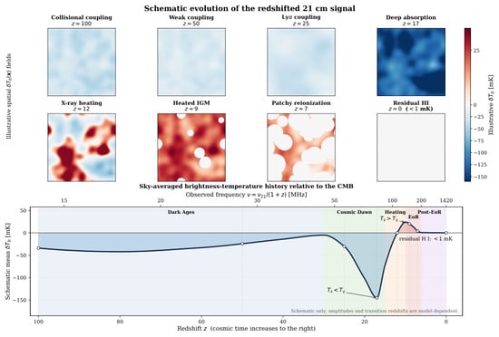
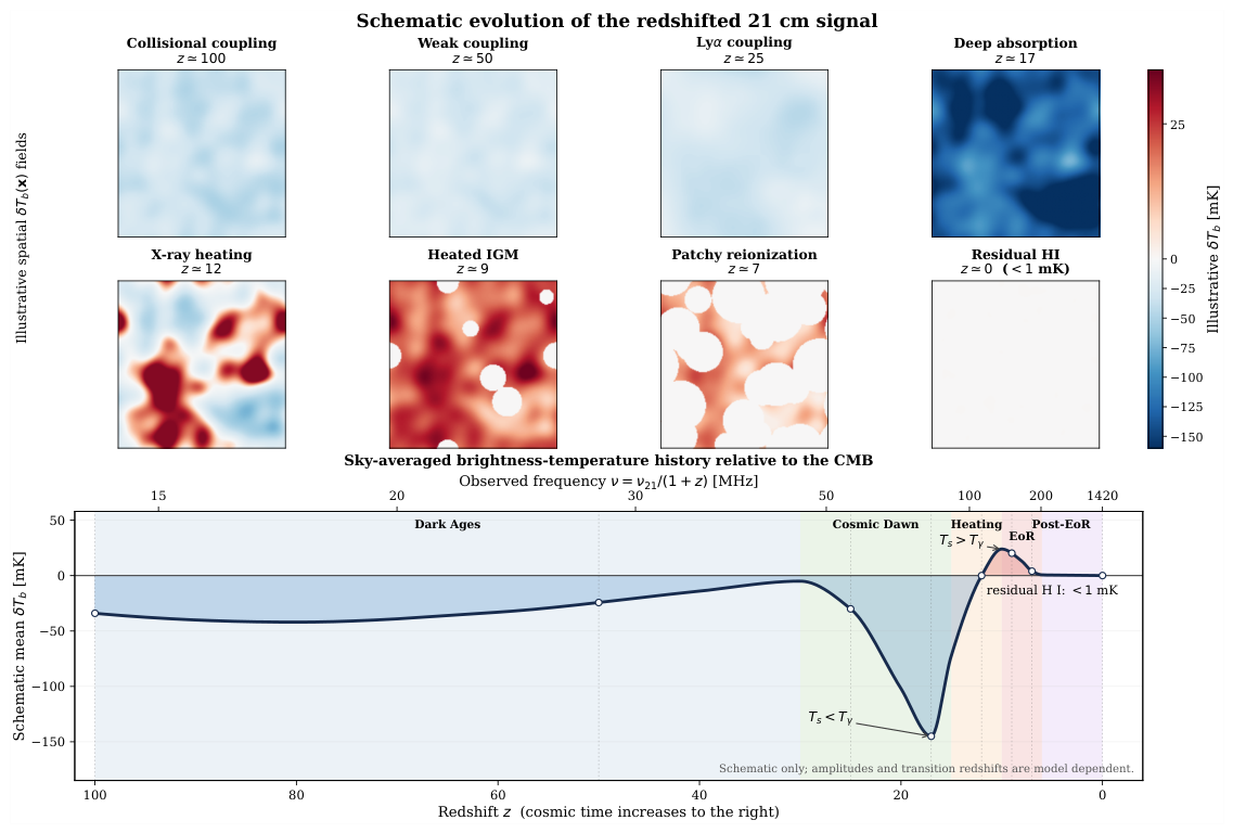
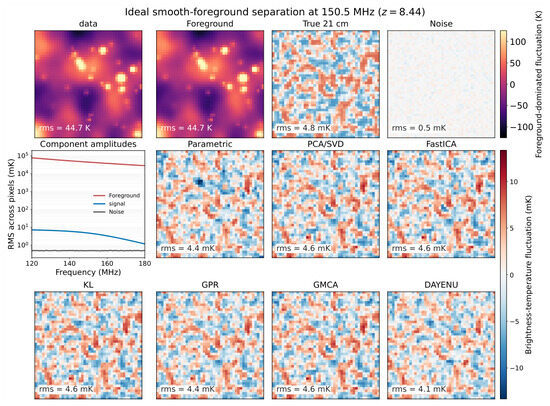
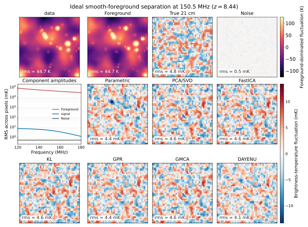
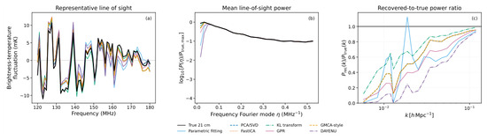
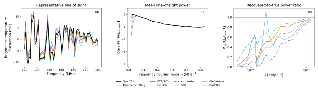
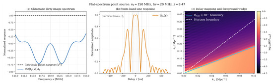
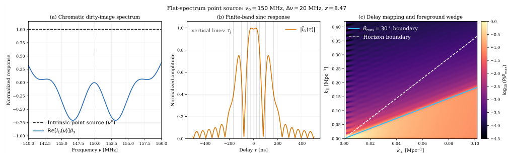
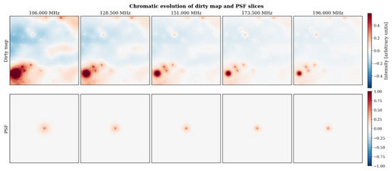
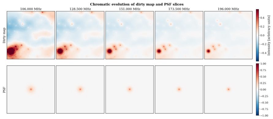
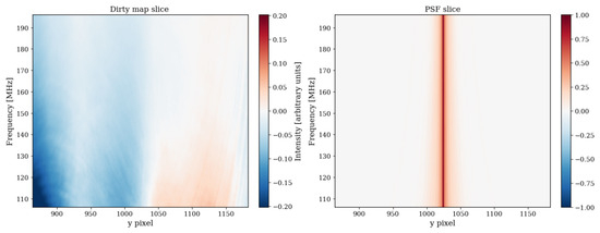
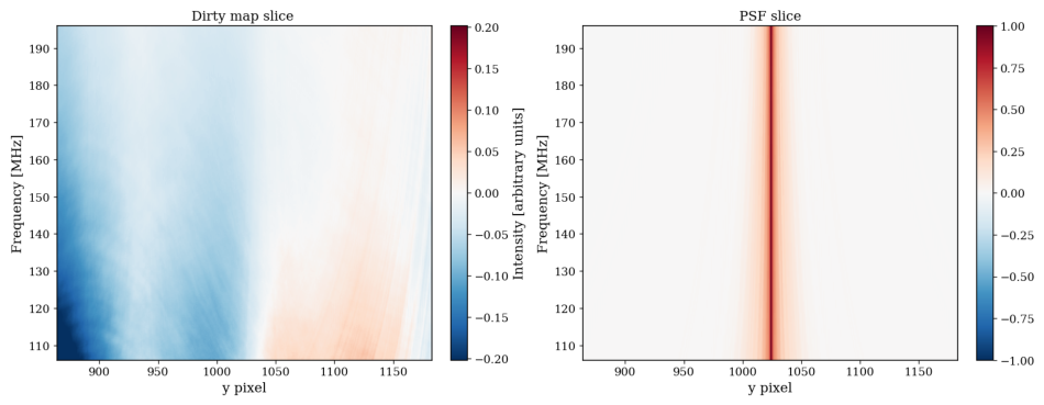
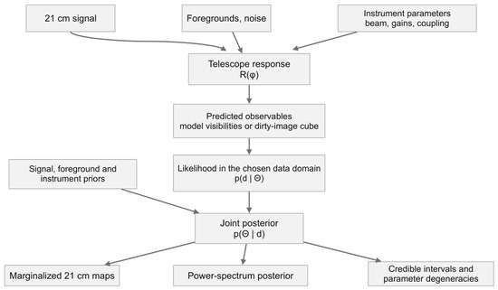
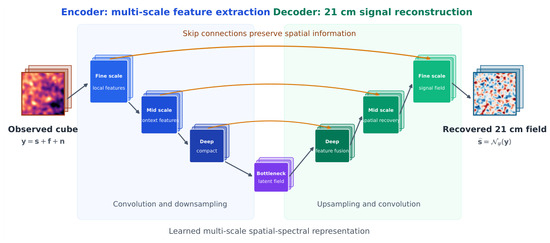

Disclaimer/Publisher’s Note: The statements, opinions and data contained in all publications are solely those of the individual author(s) and contributor(s) and not of MDPI and/or the editor(s). MDPI and/or the editor(s) disclaim responsibility for any injury to people or property resulting from any ideas, methods, instructions or products referred to in the content. |
© 2026 by the author. Licensee MDPI, Basel, Switzerland. This article is an open access article distributed under the terms and conditions of the Creative Commons Attribution (CC BY) license.