Continuously Tunable Frequency and Phase Biquad Oscillator

Abstract

This paper presents an improvement to the performance of a biquad oscillator, which is a recursive oscillator known for its excellent long-term stability. However, a significant limitation is that the oscillation frequency cannot be changed while the system is operating. Directly changing the frequency during operation causes the amplitude of the generated signal to vary significantly, either increasing or decreasing. A zero-input response analysis is used to understand the cause of this problem and to develop a solution that allows the amplitude of the generated signal to remain constant even when the oscillation frequency is changed during operation. In addition, this paper presents a method for controlling the phase of the generated signal by using a 1st-order IIR phase shifter structure. The proposed structure is specifically designed to allow the phase of the signal at the oscillation frequency to be adjusted continuously and independently of the frequency parameter. This integrated oscillator enables real-time, independent control of both signal frequency and phase without amplitude drift, making it suitable for applications requiring precise and dynamic signal synthesis.

1. Introduction

Oscillator circuits are fundamental components that play a critical role in a wide range of electronic and telecommunications systems. These include wireless communication systems, radar signal processing, and biomedical sensing systems, as well as electronic audio and music applications.

As communication and signal processing systems have fully transitioned to the digital domain, Numerically Controlled Oscillators (NCOs) or Direct Digital Synthesizers (DDS/DDFS) have become essential for generating high-precision signals with rapid frequency agility. However, traditional DDS architectures typically rely on lookup tables (LUT/ROM) for phase-to-amplitude mapping, which leads to a significant increase in memory size and negatively impacts both silicon area and power consumption. To address these limitations, numerous studies have proposed ROM-less DDS approaches that utilize computation instead of data storage. These methods include the use of IIR resonators [1], polynomial approximation [2], cosine octuple-angle combined with error compensation [3], non-uniform piecewise linear approximation [4], and recursive trigonometric techniques [5]. These techniques effectively reduce memory requirements while simultaneously enhancing the precision and overall efficiency of the system.

To address the aforementioned limitations, Recursive Oscillators have gained widespread interest due to their ability to generate sine waves using low-order difference equations while requiring minimal computational resources. Various structures exist, such as Direct-form and Coupled-form [6], each presenting different advantages and constraints regarding complexity, resolution, and coefficient sensitivity—particularly when generating low-frequency signals [7] and sensitivity to quantization [8]. However, a significant drawback of these structures is the accumulation of numerical errors, which impacts signal stability and purity [9]. Consequently, the Biquad Oscillator structure has garnered attention because of its simple architecture and its capacity to be designed for high stability and practical implementation. It has been effectively utilized in biomedical measurement systems, such as bio-impedance measurement [10].

However, the biquad oscillator still has an important limitation. When the oscillation frequency is changed, the amplitude of the generated signal also changes accordingly. This effect becomes more pronounced when the new frequency differs significantly from the original frequency, resulting in amplitude instability caused by the behavior of the recursive system itself. In previous work by the authors, zero-input response (ZIR) analysis was introduced to explain this mechanism and to propose a compensation method that allows the biquad oscillator to adjust its frequency online while maintaining constant amplitude [11].

Furthermore, the ability to control the phase of oscillating signals is a core pillar of modern signal processing. Phase shifters serve as fundamental components widely used in applications such as phase modulation or Phase Shift Keying (PSK) in communication systems, as well as creating phaser effects in audio and music processing. While most research is based on all-pass filters, multi-phase oscillators with adjustable phase values were presented in [12]; however, these remain limited by their phase-shift range and their entirely analog circuitry. Digital phase shifters based on all-pass filters for audio effects were proposed in [13,14]. Additionally, digital phase shifters have been developed on FPGA platforms to provide a constant −90° phase shift using the Hilbert transformer [15], though these structures are complex and impose a significant computational burden. To address this limitation, the authors previously proposed a tunable first-order IIR phase shifter that allows the phase of a sinusoidal signal to be adjusted continuously in real time with a simple structure, making it suitable for use with digital oscillators [16].

However, this approach was presented separately from the oscillator structure. Motivated by this gap, this research proposes an integrated framework that combines frequency tuning, amplitude stabilization, and phase control within a single structure. The proposed approach extends the biquad recursive oscillator by incorporating zero-input response analysis together with a tunable first-order IIR phase shifter. As a result, a continuous frequency- and phase-tunable biquad recursive digital oscillator is obtained, which enables substantially smooth frequency and phase transitions—particularly during gradual parameter adjustments—while eliminating amplitude drift with minimal computational overhead.

The remainder of this paper is organized as follows. Section 2 reviews recursive oscillator structures and the problem of amplitude drift. Section 3 presents the proposed methods for amplitude stabilization using the ZIR analysis and phase adjustment. Section 4 provides experimental results and discussions, and Section 5 concludes the paper.

2. Biquad Recursive Oscillator: Fundamentals and Amplitude Discontinuity Under Frequency Tuning

2.1. Operating Principle, Difference Equation, and Initial Conditions

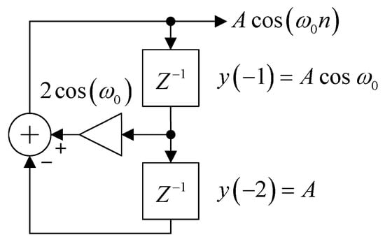
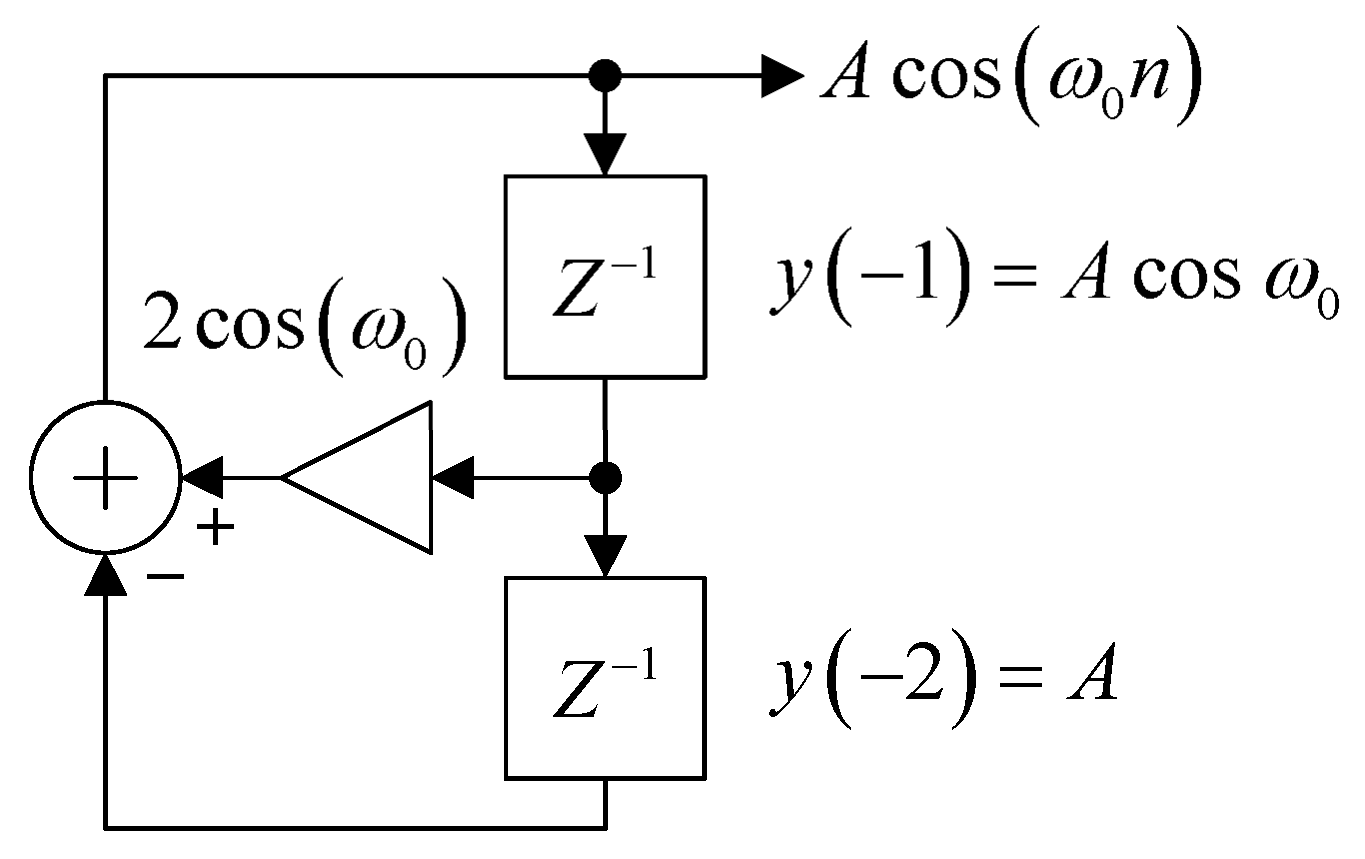
One of the recursive oscillators that is of interest due to the simplicity of its structure and related equations is the biquad oscillator, which is an all-pole second-order IIR filter without an input signal and is realized using a direct-form structure, as shown in Figure 1.

Figure 1. Biquad oscillator in direct-form structure.

The simple structure shown in Figure 1 can be described by a recursive equation with the following difference equation:

$$y(n)=2\cos ({\omega }_0)y(n-1)-y(n-2)$$

(1)

where ${\omega }_0={\displaystyle \frac{2\pi f_0}{F_s}}$, $f_0$ is the oscillating frequency (Hz) and $F_s$ is the sampling frequency (Hz).

A sinusoidal signal $y(n)$ can oscillate from this structure, where the oscillation frequency is determined by the coefficient $2\cos ({\omega }_0)$, without requiring any input signal, as shown in (1). However, initial conditions are necessary for the oscillation process. The amplitude and the initial phase of the signal are determined by these initial conditions. For the generation of a cosine signal with constant amplitude A = 1 (unity gain), the required initial conditions are given as follows [17]:

$$y(-1)=A\cos ({\omega }_0) \mathrm{and} y(-2)=A$$

(2)

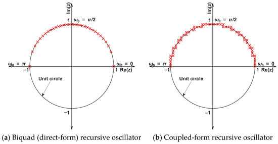
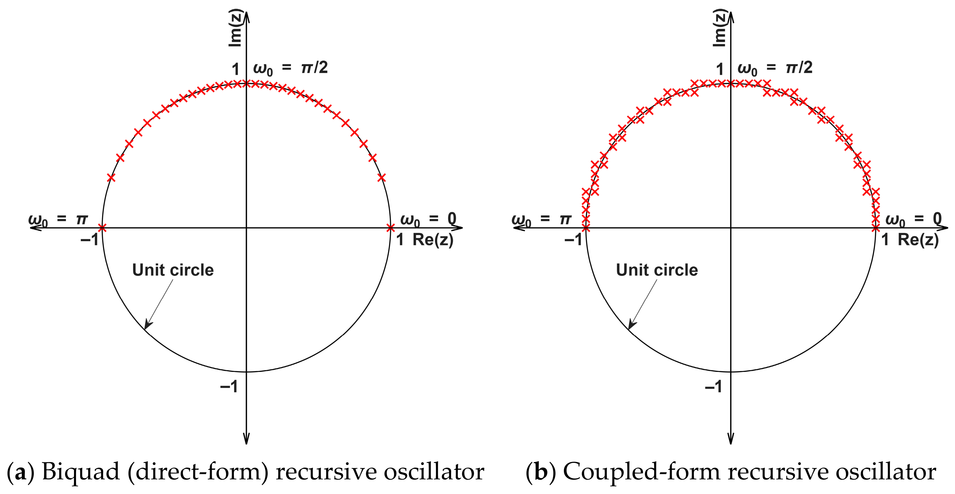
The biquad oscillator exhibits excellent long-term stability for signal generation. In an ideal mathematical model, the signal amplitude remains constant over time as the system poles lie precisely on the unit circle, as illustrated in Figure 2a. However, in practical implementations using finite-precision arithmetic, effects such as coefficient quantization and roundoff errors may cause the poles to deviate slightly from the unit circle. This deviation can result in gradual amplitude drift and oscillation frequency inaccuracies. Despite these limitations, the biquad structure remains highly suitable for digital sine wave generation due to its simplicity and practical stability.

Figure 2. Effect of 4-bit coefficient quantization on the distribution of pole locations in one quadrant of the unit circle at different oscillation frequencies; the red crosses denote the pole locations, which are shown only in the upper half of the unit circle.

Nevertheless, a significant drawback of the biquad oscillator is its inability to support on-the-fly frequency tuning. Abruptly changing the system parameters disrupts the consistency of internal states, leading to undesirable amplitude fluctuations.

In contrast, other recursive oscillators such as the coupled-form oscillator allow frequency adjustment during operation but do not possess long-term stability. As time increases, the amplitude of the oscillating signal generated by a coupled-form oscillator gradually changes (either increasing or decreasing). This occurs due to the accumulation of roundoff error, which causes the pole radius to move away from the unit circle, as illustrated in Figure 2b.

The pole locations distributed on the unit circle in Figure 2 can be examined from the denominator terms of the transfer functions in the z-domain. For the biquad oscillator with a direct-form structure, $D_1(z)$ and the second-order recursive oscillator proposed by Rader and Gold [18] with a coupled-form structure, $D_2(z)$, the corresponding equations are given in (3) and (4), respectively.

$$D_1(z)=1-2\cos ({\omega }_0)z^{-1}+z^{-2}=0$$

(3)

$$D_2(z)=1-2\cos ({\omega }_0)z^{-1}+\left({\cos }^2({\omega }_0)+{\sin }^2({\omega }_0)\right)z^{-2}=0$$

(4)

At first glance, Equation (4) appears to be equivalent to Equation (3), since the pole radius is equal to ${\cos }^2({\omega }_0)+{\sin }^2({\omega }_0)=1$, which places the poles on the unit circle. However, quantization effects and roundoff noise may accumulate over time while the oscillator is operating. This accumulated numerical error can cause the poles to move outside the unit circle, resulting in a gradual increase in the amplitude of the oscillating signal. Conversely, the poles may also move inside the unit circle, which causes the amplitude of the oscillating signal to gradually decrease over time. In contrast, for the biquad oscillator described by (3), quantization and roundoff errors cannot change the pole radius, which remains equal to one, while the pole angle may be changed, resulting in inaccuracy of oscillation frequency but stability. Therefore, the poles always remain on the unit circle. This is the reason why the biquad oscillator exhibits excellent long-term stability among recursive oscillators.

2.2. The Phenomenon of Amplitude Discontinuity

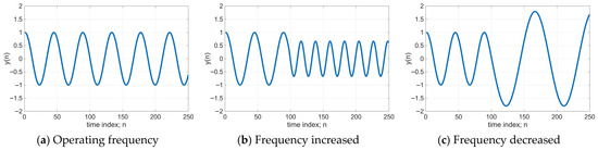
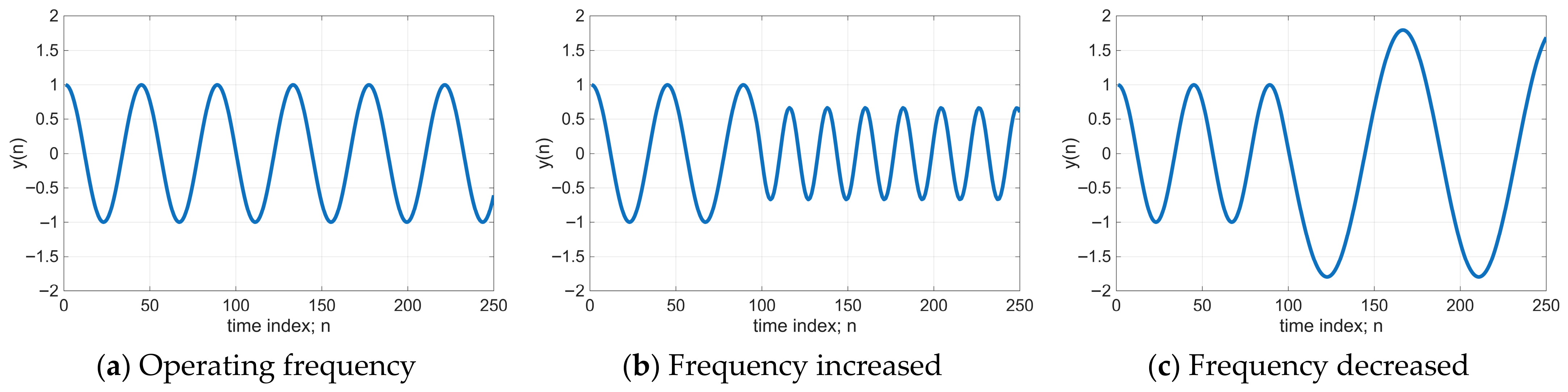
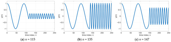
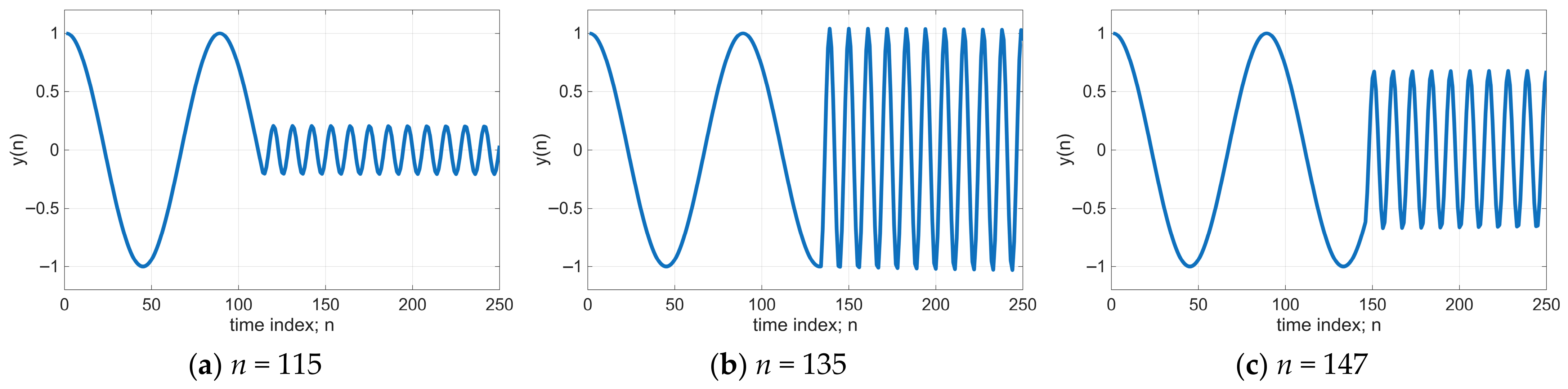
Although the biquad oscillator provides excellent long-term stability, it cannot change the oscillation frequency (${\omega }_0$) while the system is operating. In other words, the biquad oscillator is suitable only for applications with a fixed oscillating frequency or static operation. If the oscillation frequency is changed during operation by directly modifying the coefficient from $2\cos ({\omega }_0)$ to $2\cos ({\omega }_0^{\prime })$, the amplitude of the oscillating signal at the new frequency (${\omega }_0^{\prime }$) will change, either increasing or decreasing. This effect is referred to as amplitude discontinuity or amplitude drift. An example of dynamic frequency adjustment while the biquad oscillator is operating at the original oscillation frequency is illustrated in Figure 3.

Figure 3. Output waveform of the biquad recursive oscillator.

Figure 3a shows a cosine signal generated by the biquad oscillator, where the oscillation frequency and the initial conditions follow (1) and (2), respectively. Under this condition, the biquad oscillator demonstrates excellent long-term stability with a simple structure and low computational complexity. However, when the frequency is increased while the oscillator is operating at the original frequency, the amplitude of the signal at the new frequency decreases, as shown in Figure 3b. Conversely, when the new frequency is lower than the original frequency, the amplitude of the resulting signal increases.

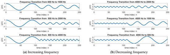
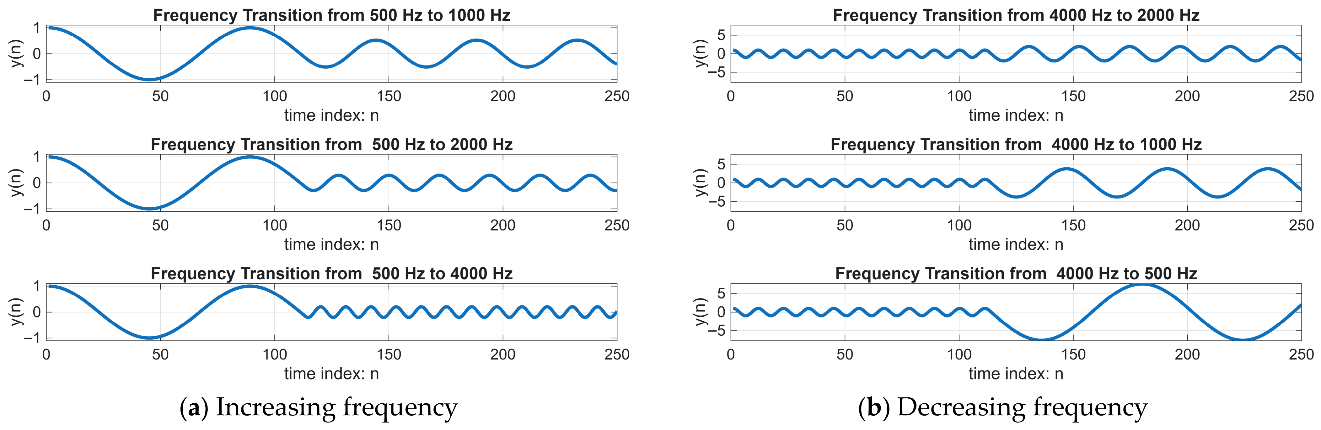
The magnitude of the frequency change also affects the amplitude variation in the signal at the new frequency, as illustrated in Figure 4.

Figure 4. Effect of the frequency difference between the original and the new frequency.

In addition, the time instant at which the frequency change occurs also affects the amplitude of the signal at the new frequency, as shown in Figure 5.

Figure 5. Effect of the time position or phase of the signal when the frequency change occurs.

From Figure 5, it can be observed that even when the new frequency is the same, if the time position or the phase of the signal at the moment of frequency change is different, the amplitude of the signal after the frequency change will also be different.

The problem of frequency adjustment during operation that affects the amplitude of the oscillating signal, as illustrated in Figure 3, Figure 4 and Figure 5, limits the practical application of the biquad oscillator. In particular, it cannot be used in applications requiring dynamic frequency adjustment, where users can change the operating frequency without restarting the system with new initial conditions. One possible approach to address this issue is to connect the oscillator with a digital automatic gain control (DAGC) system to maintain a constant amplitude even when the frequency changes. However, this method introduces other limitations, such as slow convergence time, which may cause overshoot or undershoot of the amplitude during the frequency transition. More importantly, it can introduce harmonic distortion in the sinusoidal signal generated by the oscillator. These effects will be discussed in more detail in Section 4.1, which presents the amplitude stabilization results.

In this paper, the focus is on analyzing the cause of amplitude variation in the signal generated by the biquad oscillator when the oscillation frequency is changed during operation. This phenomenon is related to the initial conditions, which no longer satisfy the conditions defined in (2) when the oscillation frequency is directly changed from $2\cos ({\omega }_0)$ to $2\cos ({\omega }_0^{\prime })$. To investigate this issue, zero-input response analysis is used, as will be discussed in Section 3. Understanding the cause of this problem leads to a systematic method for solving it.

3. The Proposed Continuously Frequency and Phase Tunable Biquad Oscillator

This section presents the conceptual framework and the main methods used to address the limitation of the biquad oscillator when the oscillation frequency is adjusted during operation. Such frequency adjustment causes the amplitude of the oscillating signal to change and lose its stability. The content of this section is divided into two subsections. The first subsection focuses on analysis using the zero-input response method to explain the structural cause of amplitude variation and to derive a compensation approach that allows the signal amplitude to remain constant even when the frequency is changed during operation. The second subsection presents the design of a 1st-order IIR filter that functions as a phase shifter. This structure is designed to operate at the specified oscillation frequency (${\omega }_0$) and allows the phase shift to be adjusted continuously without depending on the frequency parameter.

3.1. Zero-Input Response Analysis for Amplitude Stabilization

The problem of amplitude variation in the output signal when the oscillation frequency of a biquad oscillator is changed during operation motivates an analysis to determine the cause of this undesirable behavior. Based on this analysis, a solution approach is then proposed in this subsection.

Consider the difference equation of a linear time-invariant (LTI) system as follows:

$$y(n)={\displaystyle \sum _{i=0}^M{b}_{i}x(n-i)-{\displaystyle \sum _{i=1}^N{a}_{i}y(n-i)}}$$

(5)

The output $y(n)$ depends on the input $x(n)$ and the initial condition $y_0=\left[y(-1),y(-2),\dots ,y(-N)\right]$.

In theory, the complete solution $y(n)$ can be considered as the sum of the response caused by the input $x(n)$ and the response caused by the initial conditions $y_0$, as follows:

$$y(n)=y_{zi}(n)+y_{zs}(n)$$

(6)

where $y_{zi}(n)$ is the response caused by the initial conditions $y_0$ when the input $x(n)$ is assumed to be zero; therefore, it is called the zero-input response. The term $y_{zs}(n)$ is the response caused by the input $x(n)$ when the initial condition vector $y_0$ is set to zero, which is $y_{zs}(n)$ called the zero-state response. Since the biquad oscillator shown in Figure 1, has the difference equation given in (1) and has no input signal, the output $y(n)$ can be considered only as the zero-input response or $y_{zi}(n)$, as expressed in (7).

$$y(n)=y_{zi}(n)=2\cos ({\omega }_0)y(n-1)-y(n-2)$$

(7)

From (7), the characteristic equation in the z-domain can be written as

$$a(z)=z^2-2\cos ({\omega }_0)z+1=0$$

(8)

The roots of the characteristic equation in (8) represent the pole locations of the biquad oscillator, which form a pair of complex conjugate poles. Equation (8) has the same form as Equation (3), which was discussed earlier in Section 2.1.

In general, for a complex-mode zero-input response, where the poles are a pair of complex conjugates $p_{1,2}=r{e}^{\pm j\omega }$, with $r$ representing the pole radius and $\omega$ representing the pole angle, the response can be expressed as the sum of damped sinusoidal terms as follows.

$$y_{zi}(n)=r^n\left[c_1\cos (\omega n)+c_2\sin (\omega n)\right]$$

(9)

For the complex-conjugate poles of the biquad oscillator described by (8), the pole radius is $r=1$, and the pole angle $\omega ={\omega }_0$ corresponds to the normalized oscillating frequency, as explained in Section 2.1. Therefore, the zero-input response of the biquad oscillator can be written as

$$y_{zi}(n)=c_1\cos ({\omega }_{0}n)+c_2\sin ({\omega }_{0}n)=y(n)$$

(10)

The coefficients $c_1$ and $c_2$ in (10) depend on the initial condition vector $y_0=\left[y(-1),y(-2)\right]$. From (10), the following relations can be obtained:

$$y(-1)=c_1\cos (-{\omega }_0)+c_2\sin (-{\omega }_0)$$

(11)

$$y(-2)=c_1\cos (-2{\omega }_0)+c_2\sin (-2{\omega }_0)$$

(12)

Equations (11) and (12) can be written in matrix form as

$$\left[\begin{array}{c}y(-1)\\ y(-2)\end{array}\right]=\left[\begin{array}{cc}\cos (-{\omega }_0)& \sin (-{\omega }_0)\\ \cos (-2{\omega }_0)& \sin (-2{\omega }_0)\end{array}\right]\left[\begin{array}{c}{c}_1\\ c_2\end{array}\right]$$

(13)

From (13), it can be seen that the coefficients $c_1$ and $c_2$ can be calculated from the initial conditions $y_0=\left[y(-1),y(-2)\right]$ by computing the inverse matrix, as shown in (14):

$$\left[\begin{array}{c}{c}_1\\ c_2\end{array}\right]={\left[\begin{array}{cc}\cos (-{\omega }_0)& \sin (-{\omega }_0)\\ \cos (-2{\omega }_0)& \sin (-2{\omega }_0)\end{array}\right]}^{-1}\left[\begin{array}{c}y(-1)\\ y(-2)\end{array}\right]$$

(14)

Equation (14) shows that the initial conditions $y(-1)$ and $y(-2)$ of the biquad oscillator determine the coefficients $c_1$ and $c_2$. When (7) and (10) are considered together, the output signal can be written as

$$y(n)=2\cos ({\omega }_0)y(n-1)-y(n-2)=c_1\cos ({\omega }_{0}n)+c_2\sin ({\omega }_{0}n)$$

(15)

From this expression, it can be seen that the coefficients $c_1$ and $c_2$ determine the amplitude of the output signal $y(n)$ as expressed in

$$\left|y(n)\right|=\left|c_1\cos ({\omega }_{0}n)+c_2\sin ({\omega }_{0}n)\right|=\sqrt{c_1^2+c_2^2}$$

(16)

From the analysis results, it can be observed that the amplitude of the output signal $y(n)$ generated by the biquad oscillator depends on the initial conditions $y_0=\left[y(-1),y(-2)\right]$, which must correspond to the oscillating frequency. For example, the initial conditions defined in (2) ensure that the oscillator generates a cosine signal with frequency ${\omega }_0$ and amplitude equal to 1. However, if the initial conditions do not correspond to the oscillating frequency ${\omega }_0$, the amplitude of the generated oscillating signal will not have the correct value.

When the oscillation frequency is changed from ${\omega }_0$ to ${\omega }_0^{\prime }$ while the oscillator is operating, as discussed in Section 2.2, the initial conditions and the oscillating frequency ${\omega }_0$ are correctly defined only at the beginning of operation. During operation, when the oscillation frequency is changed to a new frequency ${\omega }_0^{\prime }$, the initial conditions associated with the new frequency correspond to the previous states (pending states) that remain from the operation at the original frequency. As a result, although the oscillator can generate the new frequency, the amplitude of the signal changes. The amplitude may increase or decrease depending on whether the new frequency is lower or higher than the original frequency used as the initial oscillation condition.

If no corrective method is applied and the operating frequency is repeatedly changed during use, the worst-case situation may cause the amplitude to increase beyond the dynamic range that can be represented in the digital system and converted by the DAC in practice. This is the reason why the biquad oscillator cannot normally be used for dynamic frequency tuning.

However, the magnitude of the amplitude variation can be calculated directly from the coefficients $c_1$ and $c_2$, as shown in (16). When the oscillator frequency is updated by switching the biquad coefficients from $2\cos ({\omega }_0)$ to $2\cos ({\omega }_0^{\prime })$, the pending states $y(-1)$ and $y(-2)$ at that specific instant still reflect the previous frequency ${\omega }_0$, thereby becoming inconsistent with the new frequency ${\omega }_0^{\prime }$. In terms of signal representation, this phenomenon can be described as a mismatch between the stored state values and the basis functions of the oscillation at the new frequency. This state mismatch is the primary cause of the instantaneous amplitude discontinuities observed immediately after frequency adjustment. This situation is completely different from the initial conditions defined in (2) that are used when the oscillator starts operating at the original frequency ${\omega }_0$. Nevertheless, the new amplitude that will occur after the oscillation frequency changes to the new frequency ${\omega }_0^{\prime }$ can be predicted in advance from the pending states $\left[y(-1),y(-2)\right]$ by using (14) and (16), respectively. The reciprocal of the predicted amplitude can then be used as a compensation gain. By multiplying this compensation gain with the output signal whose amplitude has changed, the resulting signal can oscillate at the new frequency while maintaining a constant amplitude equal to the amplitude at the original frequency.

From the zero-input response analysis, a systematic method can therefore be developed to modify the biquad oscillator so that the amplitude remains constant even when the oscillation frequency is adjusted by the user during operation, as illustrated in Figure 6.

Figure 6. Result of the zero-input response analysis leading to a modification that allows the biquad oscillator to change its operating frequency while maintaining constant signal amplitude.

To reduce the complexity of computing the inverse matrix used to obtain the coefficients $c_1$ and $c_2$ from the pending states $y(-1)$ and $y(-2)$ for amplitude compensation, the matrix equation is simplified to obtain a structure that is easier to implement.

For a 2 × 2 matrix:

$$A=\left[\begin{array}{cc}a& b\\ c& d\end{array}\right]\hspace{1em}\hspace{1em}\Rightarrow \hspace{1em}\hspace{1em}{A}^{-1}={\displaystyle \frac{1}{ad-bc}}\left[\begin{array}{cc}d& -b\\ -c& a\end{array}\right]$$

(17)

From (14), we obtain

$${\left[\begin{array}{cc}\cos (-{\omega }_0)& \sin (-{\omega }_0)\\ \cos (-2{\omega }_0)& \sin (-2{\omega }_0)\end{array}\right]}^{-1}={\displaystyle \frac{1}{\cos (-{\omega }_0)\sin (-2{\omega }_0)-\sin (-{\omega }_0)\cos (-2{\omega }_0)}}\times \left[\begin{array}{cc}\sin (-2{\omega }_0)& -\sin (-{\omega }_0)\\ -\cos (-2{\omega }_0)& \cos (-{\omega }_0)\end{array}\right]$$

(18)

Using the following trigonometric identities,

$$\begin{array}{ccccccc}\cos (-{\omega }_0)\hfill & =\hfill & \cos ({\omega }_0)\hfill & \hfill & \sin (-2{\omega }_0)\hfill & =\hfill & -\sin (2{\omega }_0)\hfill \\ \hspace{0.33em}\sin (2{\omega }_0)\hfill & =\hfill & 2\sin ({\omega }_0)\cos ({\omega }_0)\hfill & \hfill & \hspace{0.17em}\hspace{0.33em}\cos (2{\omega }_0)\hfill & =\hfill & 2{\cos }^2({\omega }_0)-1\hfill \end{array}$$

(19)

Equation (18) can be rewritten as

$${\left[\begin{array}{cc}\cos (-{\omega }_0)& \sin (-{\omega }_0)\\ \cos (-2{\omega }_0)& \sin (-2{\omega }_0)\end{array}\right]}^{-1}=-{\displaystyle \frac{1}{\sin ({\omega }_0)}}\times \left[\begin{array}{cc}-2\sin ({\omega }_0)\cos ({\omega }_0)& \sin ({\omega }_0)\\ 1-2{\cos }^2({\omega }_0)& \cos ({\omega }_0)\end{array}\right]$$

(20)

Therefore,

$${\left[\begin{array}{cc}\cos (-{\omega }_0)& \sin (-{\omega }_0)\\ \cos (-2{\omega }_0)& \sin (-2{\omega }_0)\end{array}\right]}^{-1}=\left[\begin{array}{cc}2\cos ({\omega }_0)& -1\\ {\displaystyle \frac{2{\cos }^2({\omega }_0)-1}{\sin ({\omega }_0)}}& {\displaystyle \frac{-\cos ({\omega }_0)}{\sin ({\omega }_0)}}\end{array}\right]$$

(21)

Substituting (21) into (14) gives

$$\left[\begin{array}{c}{c}_1\\ c_2\end{array}\right]=\left[\begin{array}{cc}2\cos ({\omega }_0)& -1\\ {\displaystyle \frac{2{\cos }^2({\omega }_0)-1}{\sin ({\omega }_0)}}& {\displaystyle \frac{-\cos ({\omega }_0)}{\sin ({\omega }_0)}}\end{array}\right]\left[\begin{array}{c}y(-1)\\ y(-2)\end{array}\right]$$

(22)

From (22), the following results can be obtained:

$$c_1=2\cos ({\omega }_0)y(-1) - y(-2)$$

(23)

and

$$\begin{array}{ccc}{c}_2\hfill & =\hfill & {\displaystyle \frac{1}{\sin ({\omega }_0)}}\left[\left(2{\cos }^2({\omega }_0)-1\right)y(-1) - \cos ({\omega }_0)y(-2)\right]\hfill \\ \hfill & =\hfill & {\displaystyle \frac{1}{\sin ({\omega }_0)}}\left[\cos ({\omega }_0)\left(2\cos ({\omega }_0)y(-1)-y(-2)\right) - y(-1)\right]\hfill \end{array}$$

(24)

Substituting $c_1$ into (24) results in

$$c_2={\displaystyle \frac{1}{\sin ({\omega }_0)}}\left[\cos ({\omega }_0)c_1 - y(-1)\right]$$

(25)

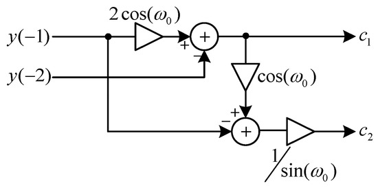
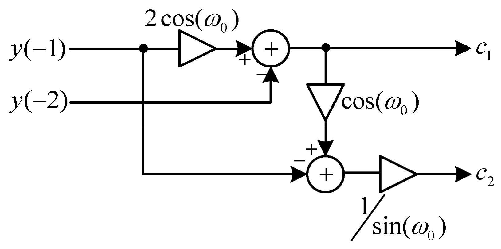
The coefficients $c_1$ and $c_2$, as shown in (23) and (25), depend on the pending states $y(-1)$ and $y(-2)$. These expressions transform the complex computation that requires the inverse matrix operation in (14) into a simpler calculation procedure that can be realized as a circuit structure, as illustrated in Figure 7.

Figure 7. Computational structure based on (14) after inverse matrix simplification.

The inverse matrix simplification makes the computation of the coefficients $c_1$ and $c_2$ in (14), which are required for calculating the compensation gain used to stabilize the signal amplitude as shown in Figure 6, easier to implement through the structure illustrated in Figure 7.

Furthermore, from the recursive difference equation of the biquad oscillator in (1), when considering the case at time n = 0, it can be observed that the calculation of $y(n)$ is identical to the calculation of $c_1$ in (23). Therefore,

$$c_1=y(n)$$

(26)

and

$$c_2={\displaystyle \frac{1}{\sin ({\omega }_0)}}\left[\cos ({\omega }_0)y(n) - y(n-1)\right]$$

(27)

In practice, both $c_1$ and $c_2$ are functions of both the time variable n and the oscillating frequency ${\omega }_0$, that is $c_1(n,{\omega }_0)$ and $c_2(n,{\omega }_0)$, respectively.

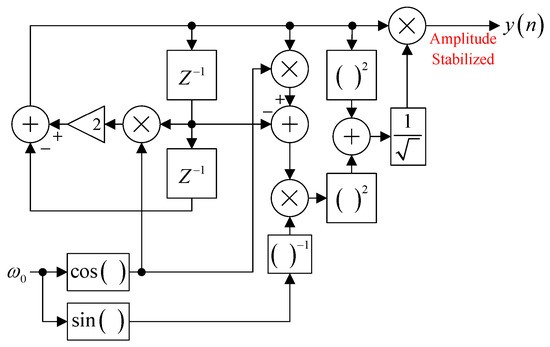
Based on Figure 6, (26) and (27) can be realized and connected to the original structure of the biquad oscillator shown in Figure 1. With this modification, the user can adjust the oscillating frequency ${\omega }_0$ online, while the amplitude of the oscillating signal after the frequency change can be stabilized so that it remains constant. This is achieved by using the values of $c_1$ and $c_2$ obtained from (26) and (27) as the compensation gain to stabilize the amplitude, as shown in (28).

$$G({\omega }_0)={\displaystyle \frac{1}{\sqrt{c_1^2(n,{\omega }_0)+c_2^2(n,{\omega }_0)}}}$$

(28)

The computation of compensation values can be sensitive to numerical errors when the coefficients $c_1$ and $c_2$ are extremely small. Such conditions may lead to an escalation of the compensation magnitude, thereby amplifying quantization and roundoff errors within finite-precision arithmetic. However, in the proposed method, $c_1$ and $c_2$ are derived directly from the system states, which are governed by oscillatory signals with bounded amplitudes. Consequently, $c_1$ and $c_2$ remain within a range comparable to the signal amplitude and do not vanish during normal operation. As a result, the denominator of (28) remains within an acceptable range, ensuring that the calculated compensation values exhibit minimal fluctuation and maintain sufficient precision for practical implementation.

It should be noted that the compensation gain in (28) is a function of the oscillating frequency only and does not depend on the time variable n. This means that the compensation gain changes only when ${\omega }_0$ is changed. Even though the time variable n continuously changes, meaning that $c_1$ and $c_2$ also vary with n, as long as the system continues oscillating at that frequency, the sum of $\sqrt{c_1^2+c_2^2}$ remains constant over time.

From the zero-input response analysis presented above, the original biquad oscillator in Figure 1 can be modified by adding an amplitude stabilization structure. As a result, the oscillator can operate as a continuous frequency-tunable biquad oscillator. The modified structure is shown in Figure 8.

Figure 8. Continuously frequency tunable biquad oscillator with amplitude stabilization structure.

The system, as presented in Figure 8, shows that the added amplitude stabilization component can instantly stabilize the amplitude when the oscillator frequency changes, thus avoiding the convergence time problem encountered in DAGC, which uses a feedback loop structure for amplitude maintenance. A comparison of the operation between the circuit presented in Figure 8 and the DAGC application will be presented in Section 4.

In addition, the amplitude stabilization block added in Figure 8 does not need to operate at every sample n. This is because the compensation gain ($G({\omega }_0)$) changes only when the oscillating frequency is modified. Therefore, after the frequency change is completed, the compensation gain ($G({\omega }_0)$) can be latched into some register, and the additional computation block for amplitude stabilization can be temporarily disconnected to reduce the computational load of calculating the compensation gain ($G({\omega }_0)$) at every signal sample. The additional computation block will be reconnected only when the user changes the oscillating frequency again. At that moment, a new compensation gain will be calculated and stored in the small memory register for use during operation. This process can be repeated whenever the oscillating frequency is adjusted during system operation.

3.2. Tunable 1st Order IIR Phase Shifter

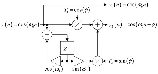
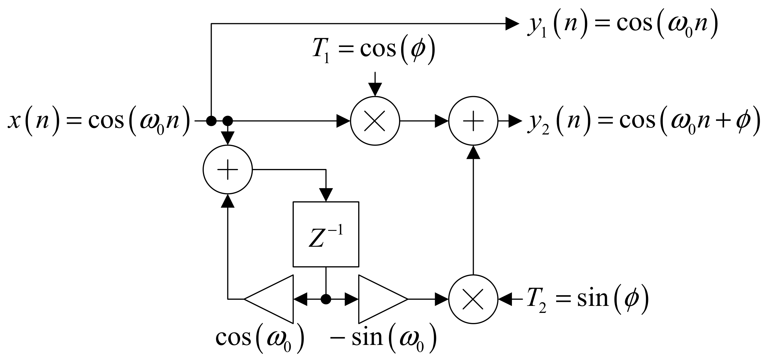
To enhance the functionality of the improved biquad oscillator so that its oscillating frequency can be adjusted during operation without affecting the signal amplitude, this work proposes a method for controlling the initial phase of the oscillating signal so that it can be continuously adjusted (continuously phase-tuned). This approach is based on the design and application of a 1st-order IIR filter that operates as a phase shifter, which is specifically designed for sinusoidal signals generated by the oscillation process. Based on this concept, this study presents the formulation of the 1st-order IIR phase shifter equation and illustrates its operational structure using a block diagram in order to explain the phase control mechanism and its suitability for use together with the biquad oscillator.

The design of the 1st-order IIR phase shifter is based on a discrete-time cosine signal with a phase shift $\cos \left({\omega }_{0}n+\varphi \right)$, which can be represented in terms of its corresponding z-transform pair [19] as follows,

$$\cos \left({\omega }_{0}n+\varphi \right)\leftrightarrow {\displaystyle \frac{\cos \varphi -\cos \left({\omega }_0-\varphi \right)z^{-1}}{1-2\cos {\omega }_0{z}^{-1}+z^{-2}}}$$

(29)

To separate the roles of oscillation generation and phase shifting, the expression in the z-domain can be rearranged by factorization as

$${\displaystyle \frac{\cos \varphi -\cos \left({\omega }_0-\varphi \right)z^{-1}}{1-2\cos {\omega }_0{z}^{-1}+z^{-2}}}={\displaystyle \frac{1-\cos {\omega }_0{z}^{-1}}{1-2\cos {\omega }_0{z}^{-1}+z^{-2}}}\times {\displaystyle \frac{\cos \varphi -\cos \left({\omega }_0-\varphi \right)z^{-1}}{1-\cos {\omega }_0{z}^{-1}}}$$

(30)

The first term on the right-hand side of (30) corresponds to the z-transform pair of a discrete-time cosine oscillator with angular frequency ${\omega }_0$, as shown in

$$\cos \left({\omega }_{0}n\right)\leftrightarrow {\displaystyle \frac{1-\cos {\omega }_0{z}^{-1}}{1-2\cos {\omega }_0{z}^{-1}+z^{-2}}}$$

(31)

This oscillator signal corresponds to the signal generated from the improved biquad oscillator, which allows frequency tuning during operation. The phase control can then be achieved by the second term in (31), which performs the phase-shifting function. This term can be defined as the transfer function of a 1st-order IIR phase shifter as follows

$$D\left(z\right)={\displaystyle \frac{\cos \varphi -\cos \left({\omega }_0-\varphi \right)z^{-1}}{1-\cos {\omega }_0{z}^{-1}}}$$

(32)

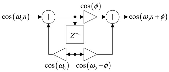
From (32), it can be seen that the structure is a 1st-order IIR filter, specifically designed to provide phase shifting for a cosine signal at frequency ${\omega }_0$ without affecting the amplitude of the output signal. The Direct Form II realization of this structure is illustrated in Figure 9.

Figure 9. Direct Form II realization of the 1st-order IIR phase shifter.

Since the input signal is sinusoidal, the 1st-order IIR phase shifter defined in (32) and illustrated in Figure 9 can provide phase shifting in both phase-lag [−180, 0] and phase-lead [0, +180] ranges. However, this design still has an important limitation in the context of online or real-time processing. Specifically, when the desired phase changes, the filter coefficients must be recalculated each time. As a result, the structure cannot efficiently support continuous phase adjustment.

To address this limitation, this study proposes a continuously tunable phase approach for the 1st-order IIR phase shifter. The approach begins by rearranging the transfer function $D\left(z\right)$ in (32) into a form that separates the dependence between the angular frequency ${\omega }_0$ and the desired phase $\varphi$, as shown in

$$D\left(z\right)={\displaystyle \frac{\cos \varphi }{1-\cos {\omega }_0{z}^{-1}}}-{\displaystyle \frac{\cos \left({\omega }_0-\varphi \right)z^{-1}}{1-\cos {\omega }_0{z}^{-1}}}$$

(33)

Considering the following trigonometric identity:

$$\cos \left(A-B\right)=\cos A\cos B+\sin A\sin B$$

(34)

The transfer function in (33) can be rewritten as

$$\begin{array}{ccc}D\left(z\right)\hfill & =\hfill & {\displaystyle \frac{\cos \varphi }{1-\cos {\omega }_0{z}^{-1}}}-\left[{\displaystyle \frac{\left(\cos {\omega }_0\cos \varphi +\sin {\omega }_0\sin \varphi \right)z^{-1}}{1-\cos {\omega }_0{z}^{-1}}}\right]\hfill \\ \hfill & =\hfill & {\displaystyle \frac{\cos \varphi \left(1-\cos {\omega }_0{z}^{-1}\right)}{1-\cos {\omega }_0{z}^{-1}}}-{\displaystyle \frac{\sin {\omega }_0\sin \varphi z^{-1}}{1-\cos {\omega }_0{z}^{-1}}}\hfill \\ \hfill & =\hfill & \cos \varphi -{\displaystyle \frac{\sin {\omega }_0\sin \varphi z^{-1}}{1-\cos {\omega }_0{z}^{-1}}}\hfill \\ \hfill & =\hfill & H_1\left(z\right)+H_2\left(z\right)\hfill \end{array}$$

(35)

This rearrangement separates the transfer function of the phase shifter into two terms. The first term, $H_1\left(z\right)$, depends only on the phase parameter $\varphi$, while the second term, $H_2\left(z\right)$, depends on both ${\omega }_0$ and $\varphi$, but parameters ${\omega }_0$ and $\varphi$ are separate. This is different from the original expression in (35), where the coefficient $\cos \left({\omega }_0-\varphi \right)$ depend on both parameters simultaneously. This property is an important factor that enables continuous phase tuning without the need to recompute all filter coefficients.

Consider $H_1\left(z\right)$ in (35), which defines the relationship between the input and output as follows

$$H_1\left(z\right)=\cos \varphi ={\displaystyle \frac{Y_1\left(z\right)}{X\left(z\right)}}$$

(36)

Transforming this expression into the time domain gives

$$y_1\left(n\right)=\cos \varphi x\left(n\right)$$

(37)

Similarly, the term $H_2\left(z\right)$ in (35) defines the relationship between the input and output as

$$H_2\left(z\right)={\displaystyle \frac{-\sin {\omega }_0\hspace{0.33em}\sin \varphi \hspace{0.33em}{z}^{-1}}{1-\cos {\omega }_0\hspace{0.33em}{z}^{-1}}}={\displaystyle \frac{Y_2\left(z\right)}{W\left(z\right)}}\times {\displaystyle \frac{W\left(z\right)}{X\left(z\right)}}$$

(38)

where

$${\displaystyle \frac{W\left(z\right)}{X\left(z\right)}}={\displaystyle \frac{1}{1-\cos {\omega }_0\hspace{0.33em}{z}^1}}$$

(39)

and

$${\displaystyle \frac{Y_2\left(z\right)}{W\left(z\right)}}=-\sin {\omega }_0\hspace{0.33em}\sin \varphi \hspace{0.33em}{z}^{-1}$$

(40)

The difference equations from (39) and (40) are articulated as

$$w\left(n\right)=x\left(n\right)+\cos {\omega }_{0}w\left(n-1\right)$$

(41)

$$y_2\left(n\right)=-\sin {\omega }_0\sin \varphi w\left(n-1\right)$$

(42)

Based on the 1st-order IIR phase shifter structure shown in Figure 9 and Equation (32), parameter updates—even at a constant frequency—require the recomputation of the coefficient $\cos \left({\omega }_0-\varphi \right)$ whenever the signal phase is modified. In contrast, the proposed structure illustrated in Figure 10 and defined by Equations (37), (41) and (42) enables continuous phase adjustment directly through the parameter $\varphi$, while the oscillation frequency remains determined by the source oscillator’s parameter ${\omega }_0$. Consequently, phase tuning in the proposed design is executed via a parameter that is decoupled from the frequency-determining coefficients. This allows the phase to be adjusted independently of ${\omega }_0$ without affecting the frequency or amplitude of signal. Therefore, the proposed 1st-order IIR phase shifter is characterized as a system with independent frequency and phase control, as depicted in the operational structure in Figure 10.

Figure 10. Tunable phase structure of the 1st-order IIR phase shifter.

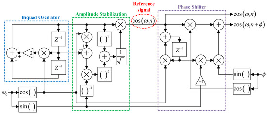
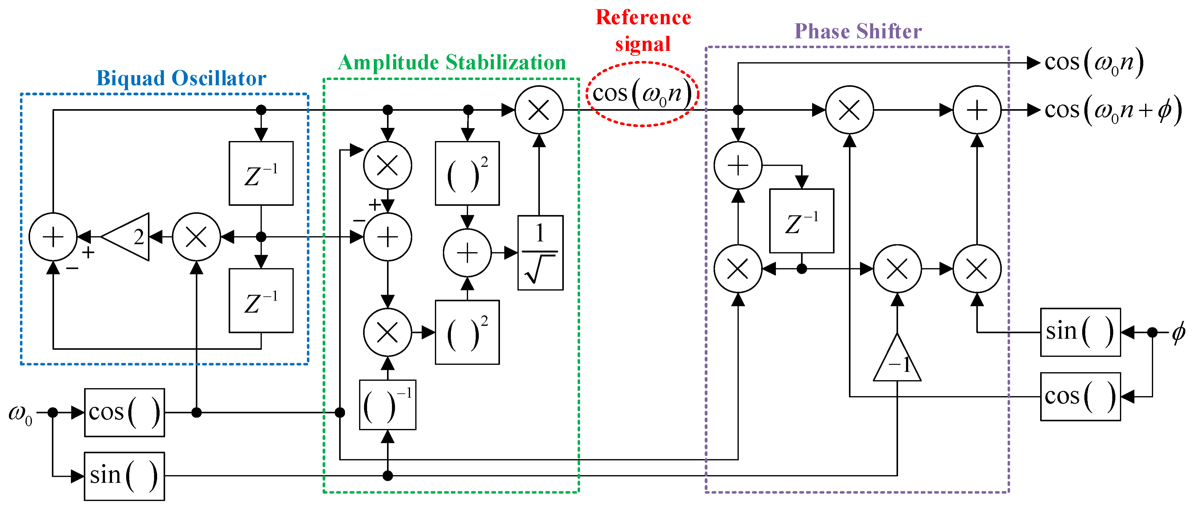
The overall system structure proposed in this research is shown in Figure 11.

Figure 11. Biquad oscillator circuit with tunable frequency and phase.

4. Results and Discussions

4.1. Amplitude Stabilization Results

This research focuses on developing a biquad oscillator structure that allows continuous frequency tuning without causing changes in the amplitude of the output signal. This approach differs from conventional methods that rely on feedback circuits such as digital automatic gain control (DAGC) to compensate for amplitude variations after frequency tuning. The novelty of this work lies in solving the problem directly at the oscillator structure level rather than compensating for the effects afterward using a feedback loop.

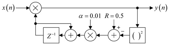
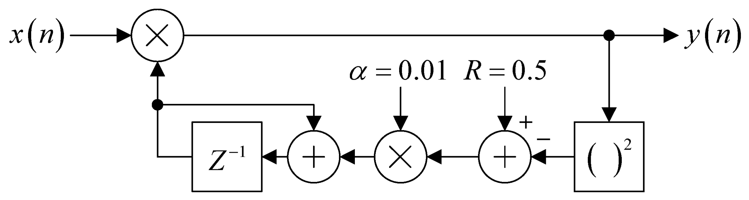
To evaluate the performance of the proposed method, a comparison was conducted with a system using DAGC, which serves as the reference approach. The structure of the DAGC system is shown in Figure 12. The experiment was divided into two cases, frequency increase and frequency decrease, in order to observe the behavior of the system under frequency changes in both directions. All experiments were performed with a sampling frequency of 44.1 kHz.

Figure 12. DAGC structure.

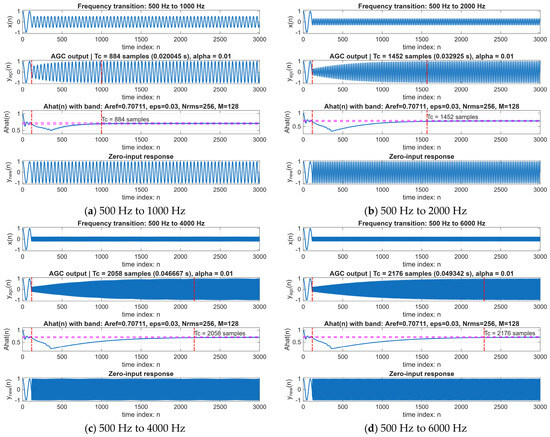
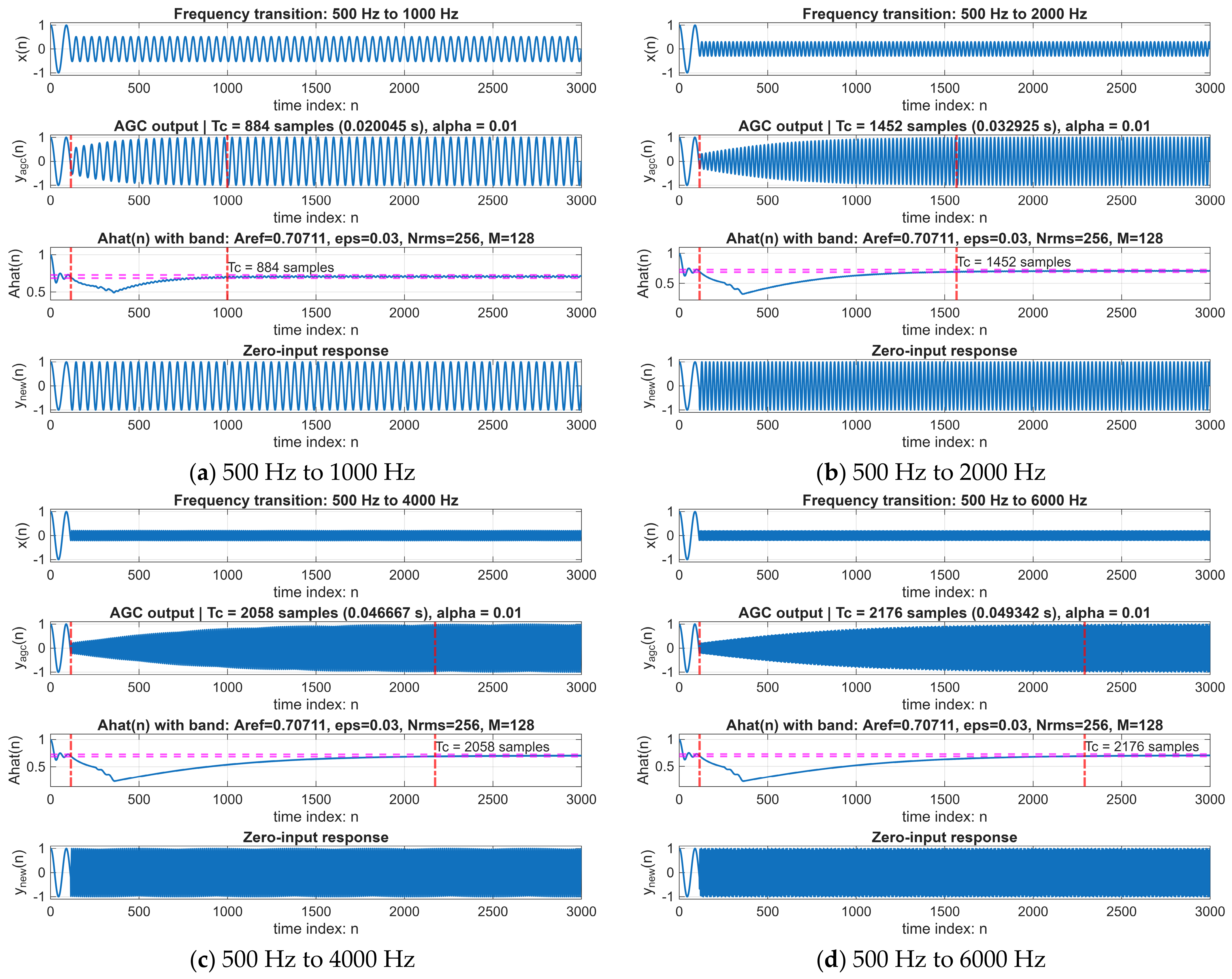
Case 1: The first experiment analyzes the effect of increasing the signal frequency. The oscillator initially operates at 500 Hz, and the frequency is then changed to 1000 Hz, 2000 Hz, 4000 Hz and 6000 Hz, respectively. In all experiments, the frequency change occurs at the time index n = 115.

Figure 13 illustrates a comparative analysis of the signal behavior as the frequency of a biquad oscillator is incremented from 500 Hz to 1000 Hz, 2000 Hz, 4000 Hz, and 6000 Hz, respectively. Each figure comprises four sub-signals: Row 1 illustrates the oscillator signal, indicating a reduction in amplitude as the frequency increases. Row 2 illustrates the outcome of employing DAGC to recalibrate the amplitude to the intended level. The vertical red dashed line indicates the convergence time ($T_c$), which is defined as the duration required for the signal to reach a steady state. Row 3 presents the estimated amplitude derived from the sliding window RMS technique. The convergence time is assessed by regarding $T_c$ as the duration required to enter the acceptable range $A_{ref}$ and persist within that range continuously. The horizontal magenta dashed line indicates the limits of the permitted range. Row 4 presents the outcomes of the proposed methodology.

Figure 13. Frequency increase cases; the red dashed lines indicate the convergence time required to reach the steady state, while the magenta dashed lines represent the tolerance band.

From Figure 13a, when the oscillator frequency changes from 500 Hz to 1000 Hz at the time index n = 115, the amplitude of the output signal suddenly decreases to approximately 0.5. When a DAGC circuit is used to compensate for this change, the signal amplitude gradually recovers and reaches a steady state at the time index n = 999, corresponding to a convergence time of 884 samples, or equivalently 884 adjustment iterations.

In contrast, the proposed method in this research maintains the signal amplitude at a constant level immediately at the moment of the frequency change, without any transient period or convergence time, unlike the DAGC-based approach.

The results shown in Figure 13b–d exhibit similar behavior. When the DAGC circuit is used to adjust the gain after the frequency change, the system still requires a convergence period to restore the signal amplitude to its steady level. It is also observed that the convergence time increases with the magnitude of the amplitude change, which reflects a limitation of amplitude control using feedback mechanisms.

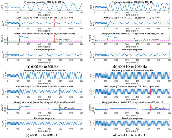
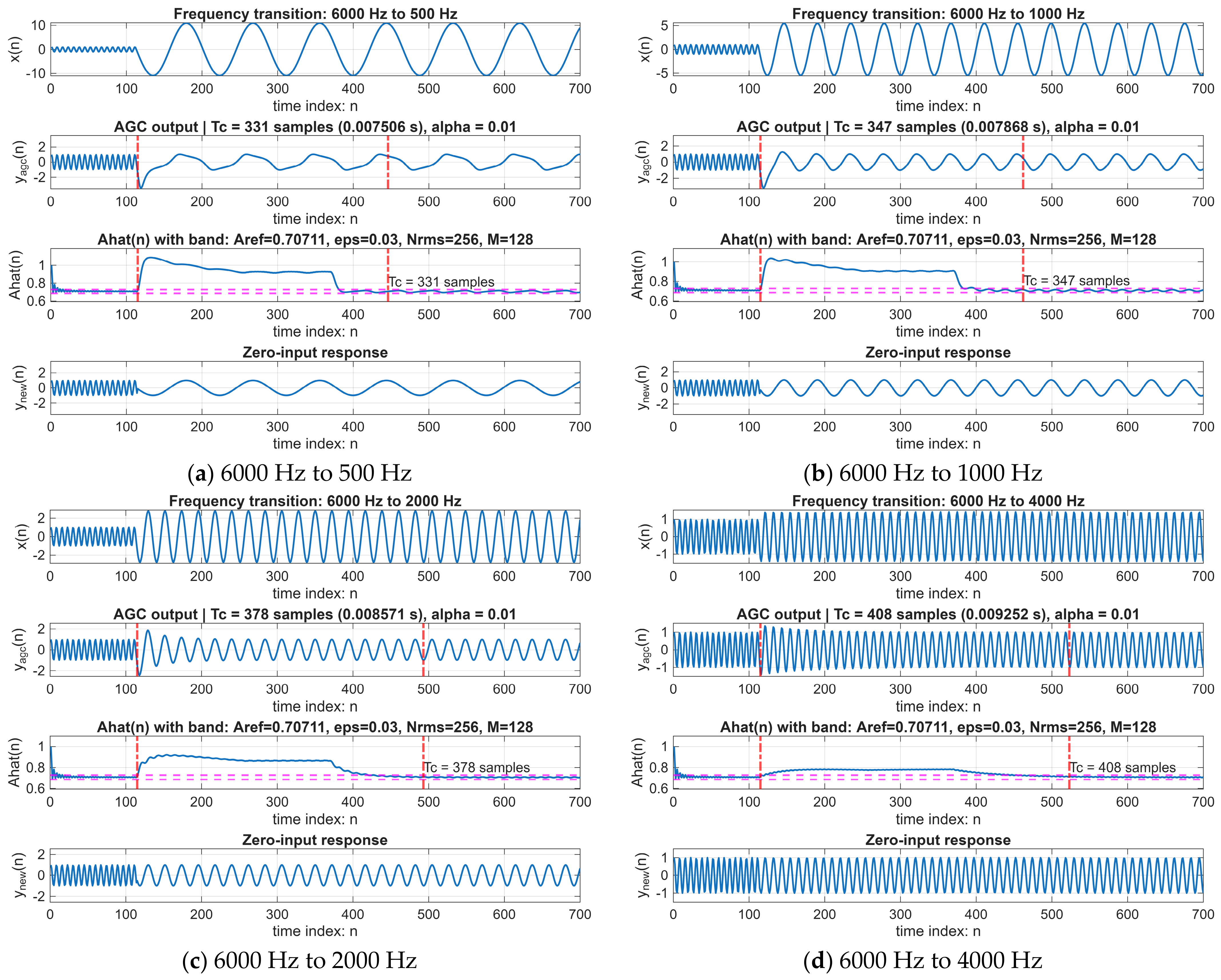
Case 2: The second experiment analyzes the effect of decreasing the signal frequency. The oscillator initially operates at 6000 Hz, and the frequency is then changed to 500 Hz, 1000 Hz, 2000 Hz and 4000 Hz, respectively. As in the previous case, the frequency change occurs at the time index n = 115 in all experiments.

Figure 14 illustrates a comparative analysis of the signal behavior as the frequency of a biquad oscillator is decreased from 6000 Hz to 500 Hz, 1000 Hz, 2000 Hz, and 4000 Hz, respectively. Each figure comprises four sub-signals, analogous to Figure 13.

Figure 14. Frequency decrease cases; the red dashed lines indicate the convergence time required to reach the steady state, while the magenta dashed lines represent the tolerance band.

Similarly, Figure 14a shows the case where the frequency changes from 6000 Hz to 500 Hz at the time index n = 115, resulting in a sudden increase in the output signal amplitude to approximately 10. When a DAGC circuit is applied to compensate for this change, the signal amplitude gradually decreases and reaches a steady state at n = 446, corresponding to a convergence time of 331 samples, or 331 adjustment iterations. However, the proposed method in this research maintains the signal amplitude at a constant level immediately at the moment of frequency change, without requiring any system adaptation period.

The results in Figure 14b–d show similar behavior, indicating that the DAGC-based approach always requires a convergence period. In contrast, the proposed method supports continuous frequency tuning without affecting the amplitude of the output signal. These results confirm the effectiveness and suitability of the proposed approach for frequency-tunable oscillators that require high amplitude stability.

Overall, the experimental results clearly demonstrate that relying on a DAGC circuit to compensate for amplitude variations caused by frequency tuning in a biquad oscillator has inherent structural limitations. DAGC operates as a nonlinear, time-varying feedback system, which means that amplitude recovery requires a convergence period that depends on the magnitude of the amplitude change and the parameters of the feedback loop. During this transient period, continuous gain adjustment may also introduce waveform distortion and spectral impurity, which are undesirable characteristics for oscillators used as frequency references or carrier signal sources. In contrast, the method proposed in this research addresses the problem at its source by modifying the structure of the biquad oscillator so that the amplitude is maintained directly during frequency tuning. Nevertheless, the proposed method entails higher structural and computational complexity compared to the conventional DAGC, as it requires precise design and parameter control to achieve superior accuracy. Despite this increased overhead, the computational investment yields several significant advantages, including the ability to maintain precise amplitude without relying on feedback loops, instantaneous response without transient artifacts, and the preservation of exceptional spectral purity. As a result, both the transient period and convergence time are eliminated, and signal distortion caused by feedback mechanisms is avoided. Therefore, the results strongly confirm that the proposed approach supports continuous frequency tuning while maintaining the quality and purity of the oscillator signal, outperforming conventional DAGC-based methods.

The performance of the proposed amplitude stabilization method is evaluated against the DAGC approach by analyzing both the frequency-domain signal spectra and the Total Harmonic Distortion (THD). The THD serves as a key indicator of spectral purity and is measured both before and after frequency transitions. The experimental evaluation is categorized into two primary scenarios: (i) an increase in oscillation frequency, and (ii) a decrease in oscillation frequency, as detailed below.

Case 1: In the first scenario, the system’s performance is analyzed during an upward frequency change. The experiment assumes an initial oscillation frequency of 500 Hz, which is subsequently increased to a target frequency of 6000 Hz.

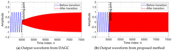
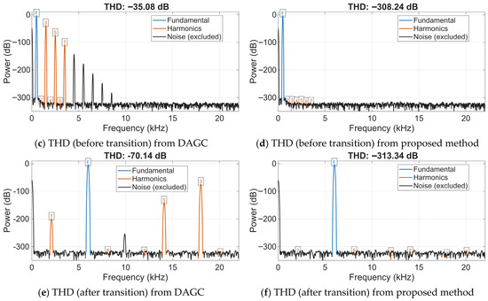
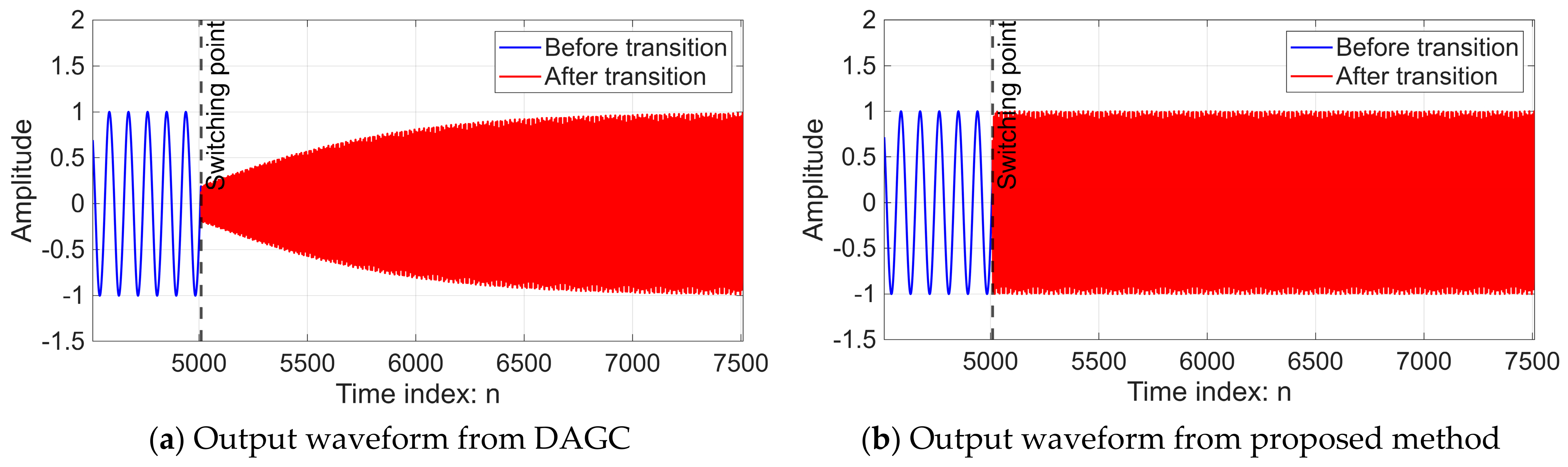
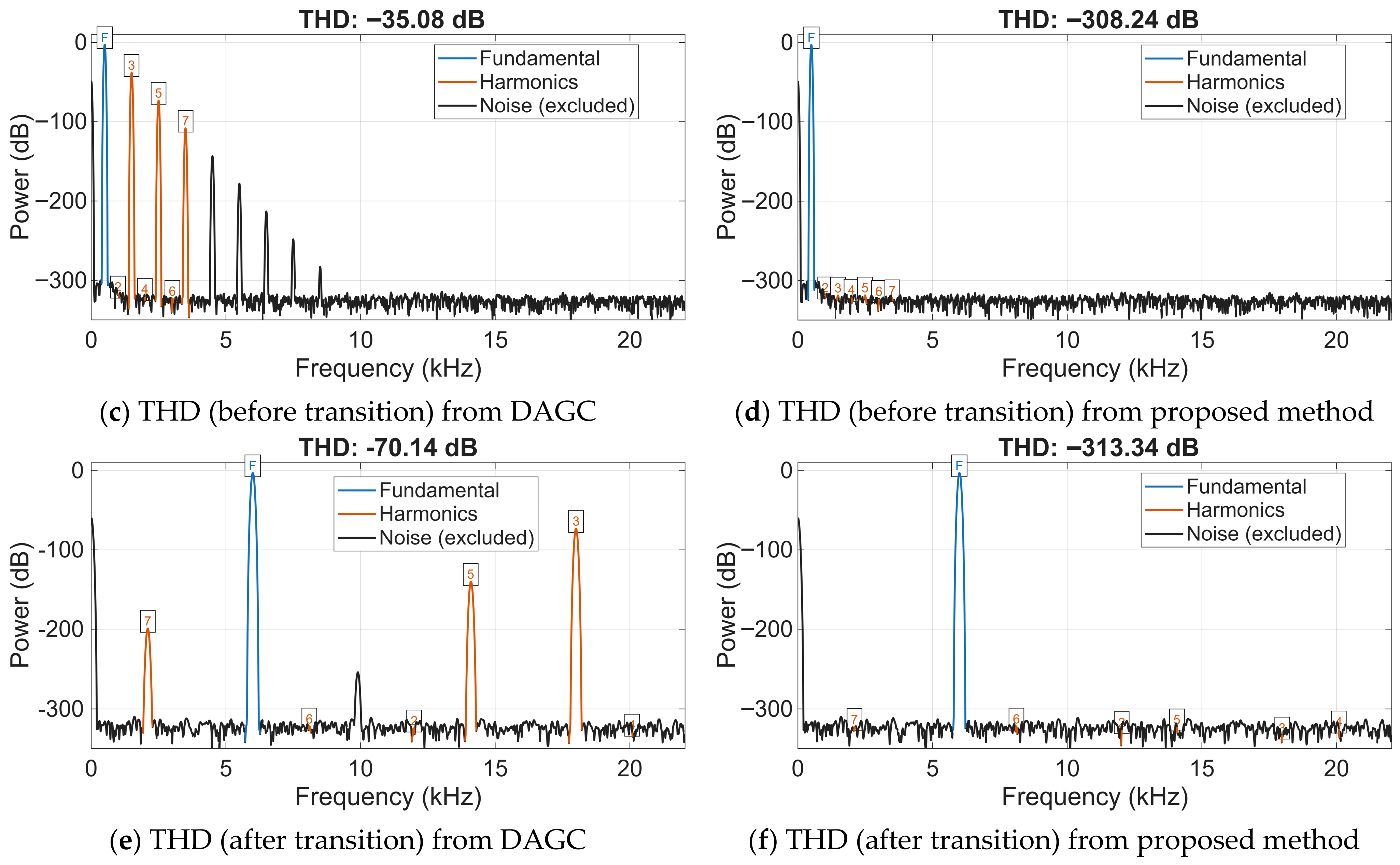
Figure 15 illustrates a comparative analysis of time-domain waveforms, frequency-domain signal spectra, and THD for a biquad oscillator during a frequency transition from 500 Hz to 6000 Hz, comparing the conventional DAGC with the proposed amplitude stabilization method. The figure is organized as follows: (a) output signal of the DAGC system; (b) output signal of the proposed system; (c) and (d) signal spectra before frequency transition for the DAGC and proposed methods, respectively; (e) and (f) signal spectra after frequency transition for the DAGC and proposed methods, respectively.

Figure 15. Comparison of time-domain waveforms and THD between DAGC and the proposed method during a frequency transition from 500 Hz to 6000 Hz; the blue label ‘F’ denotes the fundamental component, while the orange numbers denotes the harmonic orders.

In Figure 15c–f, the frequency-domain spectra are decomposed into fundamental, harmonic, and noise floor components to assess the spectral quality in each case. The corresponding performance metrics are summarized in Table 1.

Table 1. Comparison of THD before and after the frequency transition from 500 Hz to 6000 Hz.

Methods	THD Before Transition (dB)	THD After Transition (dB)
DAGC	−35.08	−70.14
Proposed method	−308.24	−313.34

Table 1 presents a comparison of THD values between the DAGC method and the proposed approach, both before and after the frequency shift from 500 Hz to 6000 Hz. For the DAGC method, the THD decreased from −35.08 dB to −70.14 dB following the transition, indicating a moderate improvement in signal quality. In contrast, the proposed method achieved significantly lower THD levels of −308.24 dB and −313.34 dB, respectively. These results demonstrate superior spectral purity and indicate that the proposed stabilization technique maintains high signal integrity more effectively than the conventional DAGC.

Case 2: In the second scenario, the system’s performance is analyzed during a downward frequency change. The experiment assumes an initial oscillation frequency of 6000 Hz, which is subsequently decreased to a target frequency of 500 Hz.

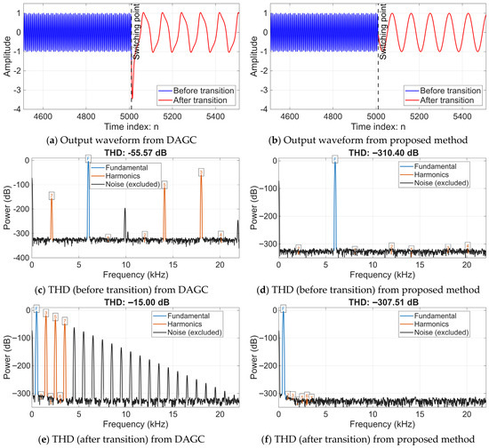
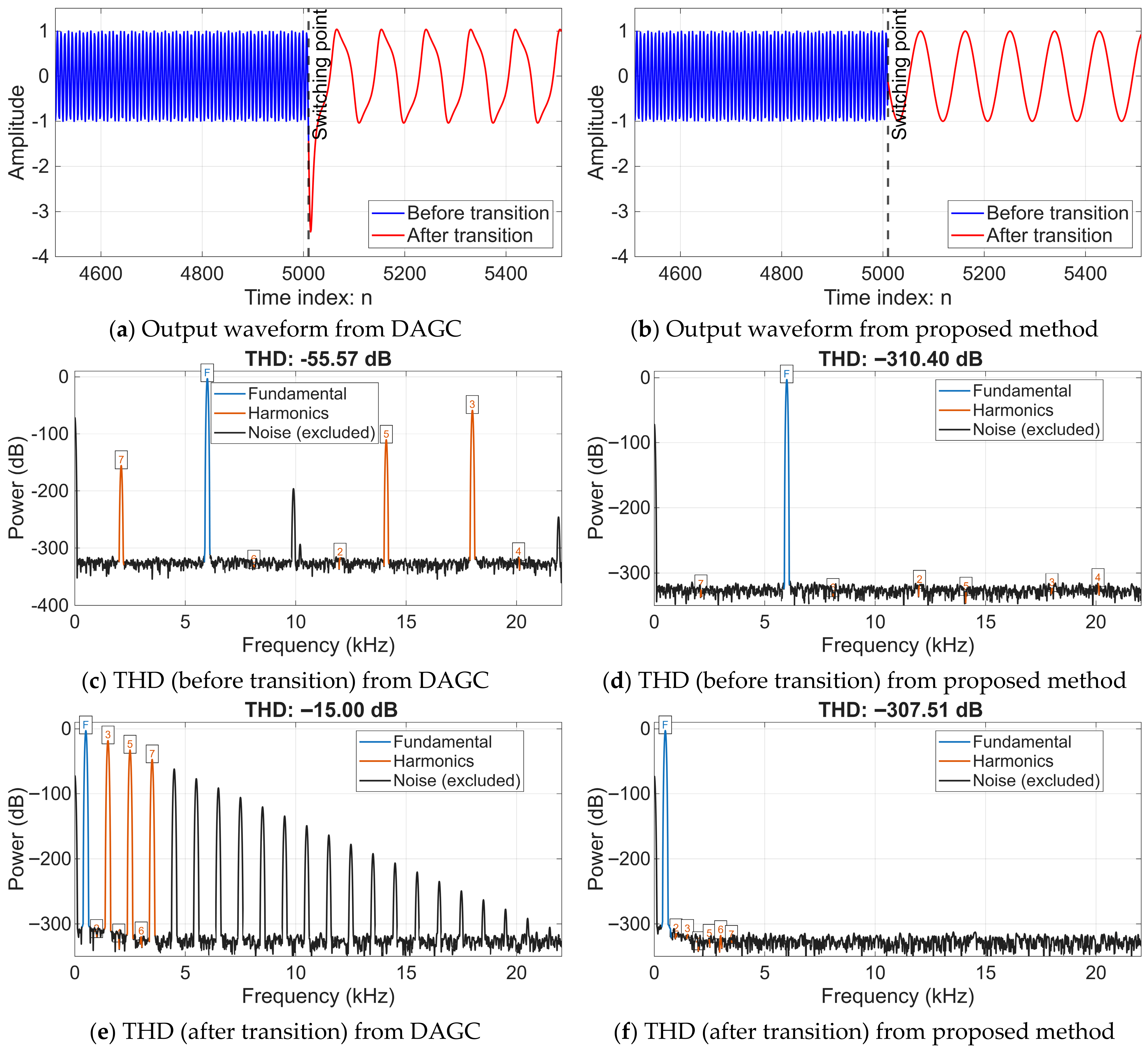
Figure 16 illustrates a comparative analysis of time-domain waveforms, frequency-domain signal spectra, and THD for a biquad oscillator during a downward frequency transition from 6000 Hz to 500 Hz. Figure 16a–f present the data in the same manner as described for Figure 15. The experimental results for this case are summarized in Table 2.

Figure 16. Comparison of time-domain waveforms and THD between DAGC and the proposed method during a frequency transition from 6000 Hz to 500 Hz; the blue label ‘F’ denotes the fundamental component, while the orange numbers denotes the harmonic orders.

Table 2. Comparison of THD before and after the frequency transition from 6000 Hz to 500 Hz.

Methods	THD Before Transition (dB)	THD After Transition (dB)
DAGC	−55.57	−15.00
Proposed method	−310.40	−307.51

Table 2 details the comparison of THD values between the DAGC method and the proposed approach during a frequency decrease from 6000 Hz to 500 Hz. For the DAGC method, the THD significantly degraded from −55.57 dB to −15.00 dB following the transition, indicating a substantial loss in signal purity. This degradation is consistent with the time-domain waveforms shown in Figure 16a, which clearly exhibit visible signal distortion. In stark contrast, the proposed method maintained remarkably low THD levels, recorded at −310.40 dB and −307.51 dB before and after the transition, respectively.

Similar to the frequency increase scenario, the proposed method consistently outperforms the DAGC in terms of spectral purity, even during a downward frequency transition. The stability of the amplitude is maintained without the convergence delays observed in the feedback-based DAGC system. The remarkably low THD values achieved by the proposed method suggest that the harmonic components are effectively suppressed near the numerical precision limits of the simulation environment.

Since the amplitude variations in a biquad oscillator—occurring when the frequency is tuned away from its initial value during operation—are dependent on the switching phase, a comprehensive investigation of all switching conditions was conducted. By analyzing the states of $y\left(n\right)$ and $y\left(n-1\right)$, the worst-case scenarios (such as peak values and zero-crossings) were identified. Analyzing these specific points is crucial because switching at a non-zero state often introduces significant energy discontinuities, leading to amplitude instability. The evaluation was performed under the following two cases:

Case 1: The effects of an upward frequency transition.

The experiment begins with an initial frequency of 500 Hz, which is subsequently increased to 1000, 2000, and 4000 Hz, respectively. Various switching phases—modeled as distinct time instances across different time indices—are applied as conditions for the frequency shift. This approach allows for the observation of amplitude behavior at the newly established frequency across all possible switching points.

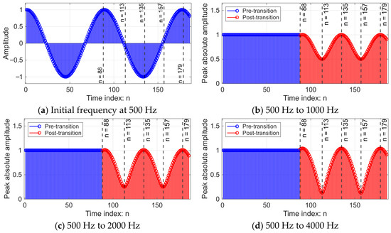
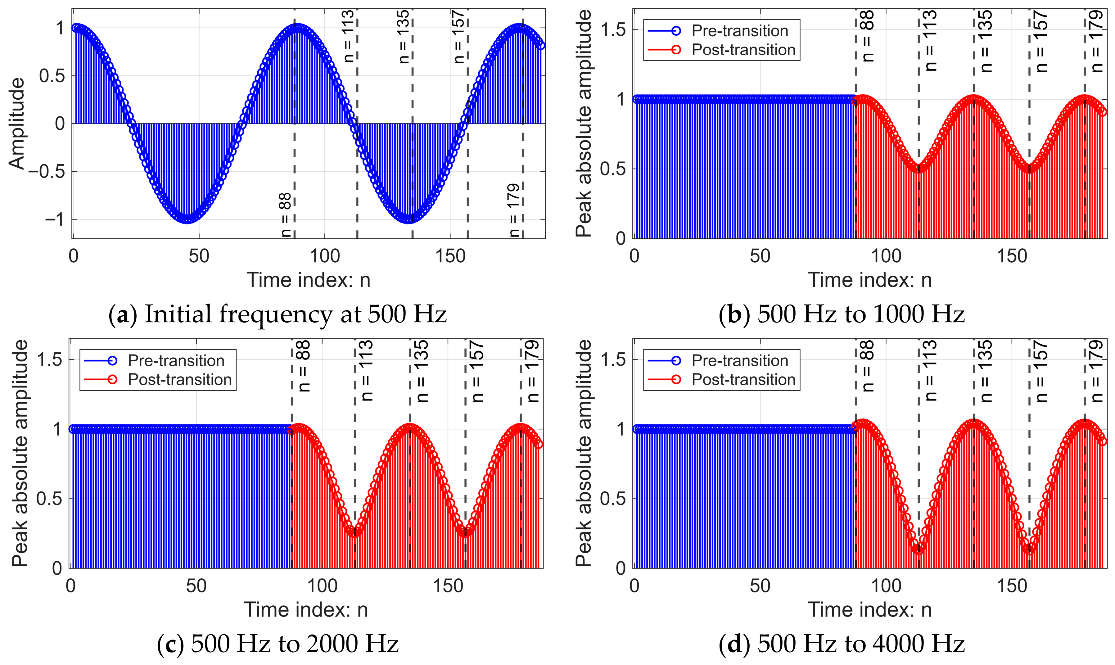
From the experimental results, as shown in Figure 17, the switching points start from n = 88 to n = 188, covering a full period of the signal, including important positions such as the peak, zero-crossing point, and the midpoint of the period. Analysis revealed that at n = 135 and n = 179, the amplitude of the signal remained almost unchanged, while at n = 113 and n = 157, the amplitude was lowest, reflecting the greatest change in amplitude. Furthermore, it was found that the amplitude of the signal after frequency switching tended to decrease significantly. In the case of a change from 500 Hz to 1000 Hz, the minimum amplitude is approximately 0.5 and decreases to approximately 0.25 and 0.125 for changes to 2000 Hz and 4000 Hz, respectively.

Figure 17. Effect of switching instant on peak amplitude variation for frequency transitions from 500 Hz to higher frequencies.

Based on the experimental results across all three cases, it is observed that the ratio between the initial and target frequencies directly dictates the degree of amplitude attenuation. Specifically, when the oscillation frequency is increased by a factor of M, the minimum amplitude is found to decrease by no more than a factor of 1/M relative to its original value.

Case 2: The effects of a downward frequency transition.

In this scenario, the oscillation frequency is decreased from an initial value of 4000 Hz to a target frequency of 2000, 1000, and 500 Hz, respectively. Similar to the previous case, the impact of various switching instances is investigated to observe the resulting amplitude variations at the lower frequency.

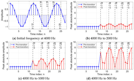
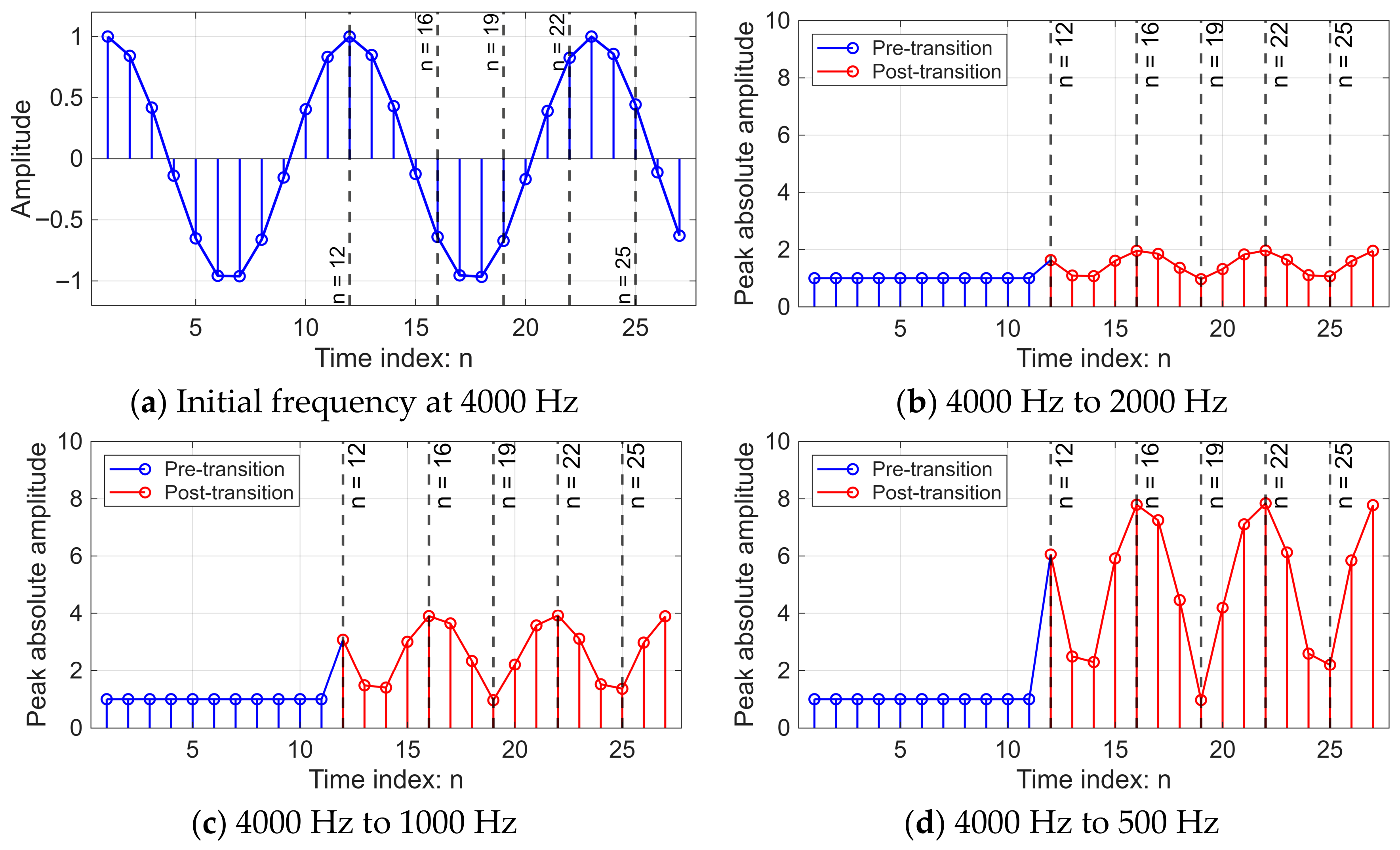
From the experiment, as shown in Figure 18, the switching points start from n = 12 to n = 27, covering a full period of the signal, including important positions such as the peak, zero-crossing point, and the midpoint of the period. Analysis revealed that at n = 16 and n = 22, the amplitude changed most drastically. Furthermore, it was found that the amplitude of the signal tended to increase significantly after frequency switching. In the case of switching from 4000 Hz to 2000 Hz, the maximum amplitude was approximately 2, increasing to approximately 4 and 8 for switching to 1000 Hz and 500 Hz, respectively.

Figure 18. Effect of switching instant on peak amplitude variation for frequency transitions from 4000 Hz to lower frequencies.

The experimental results for the frequency reduction scenarios indicate that the ratio between the initial and target frequencies maintains a direct, inverse influence on the amplitude. Specifically, when the oscillation frequency is reduced by a factor of M, the maximum peak amplitude increases by no more than M times its original value.

4.2. Tunable 1st Order IIR Phase Shifter Results

From the oscillator signal that can adjust its frequency during operation, as presented in Section 4.1, the proposed structure can be further extended to control the initial phase of the signal by using a 1st-order IIR phase shifter integrated within the same system. The user can continuously adjust the phase angle by modifying the filter coefficient, which has a direct relationship with the desired phase angle. This adjustment can be performed in real-time and does not affect the amplitude level of the signal.

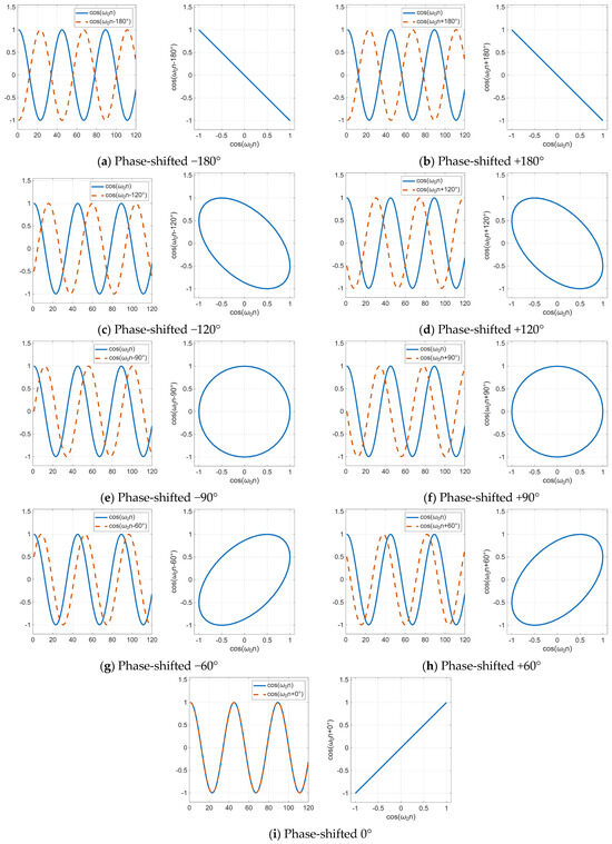
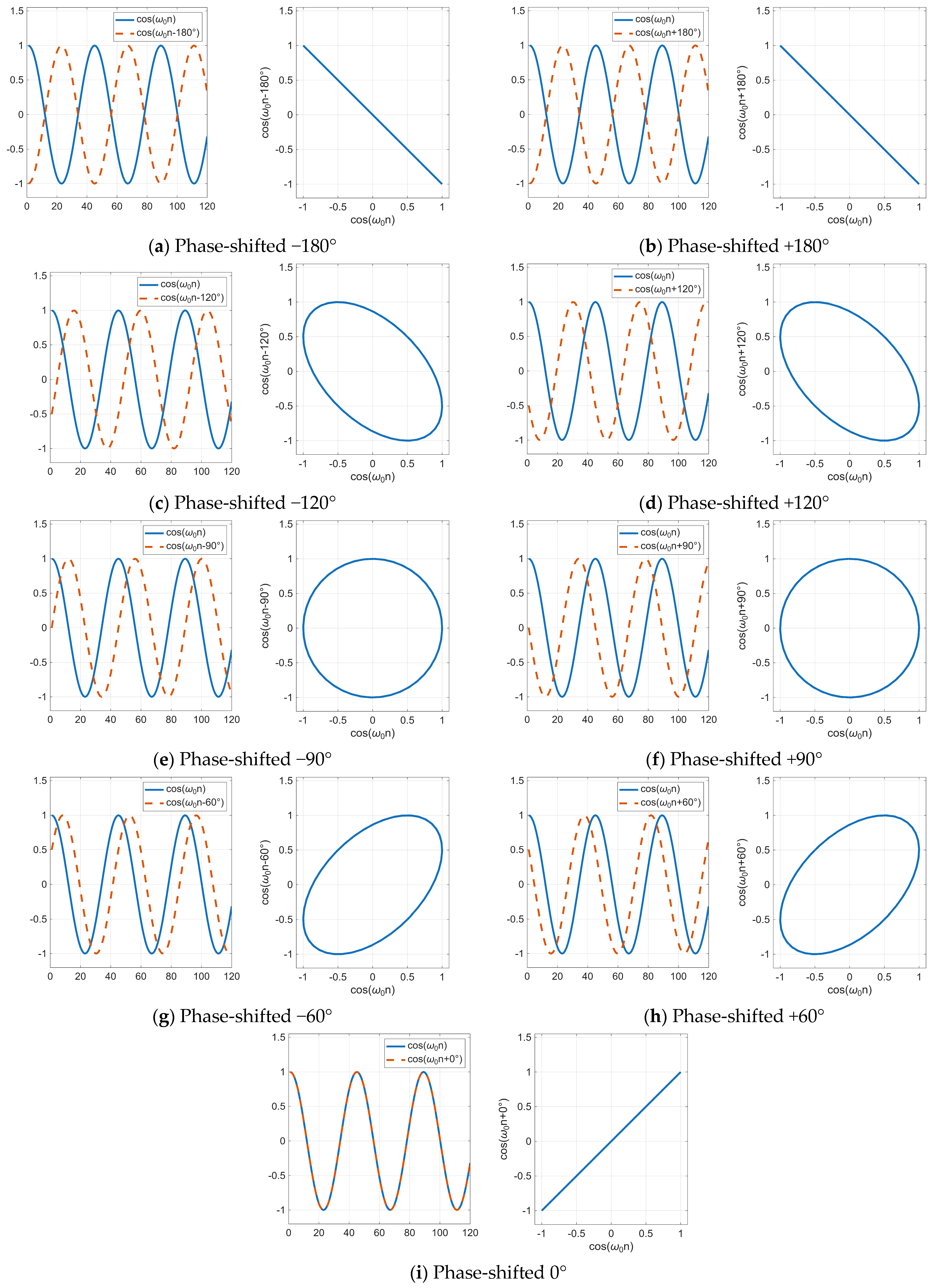
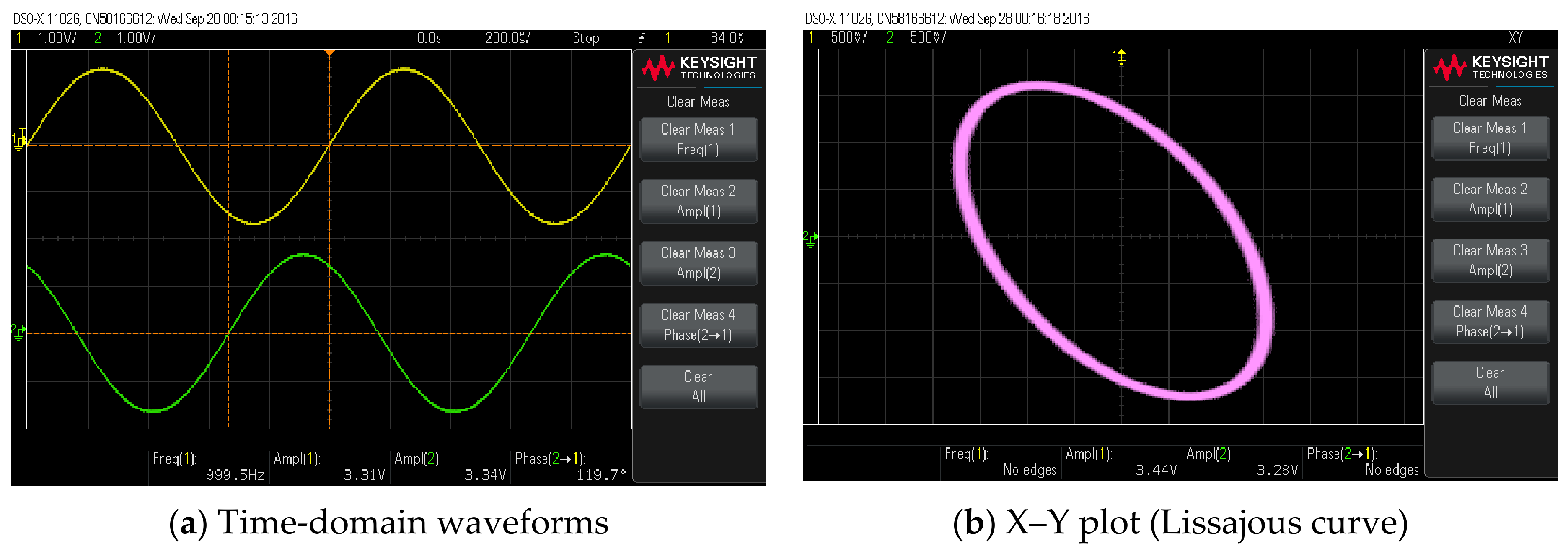
The experimental results are presented in both time-domain signals and X–Y plots (Lissajous figures) to verify the correctness of the phase shift. For different phase angles, the resulting Lissajous patterns correspond to the theoretical behavior of sinusoidal signals and demonstrate that the system can control the phase angle continuously and accurately.

Figure 19 demonstrates the performance of the proposed tunable 1st-order IIR phase shifter in both the time domain and through Lissajous patterns (x-y plots) across various phase-shift settings. In each sub-figure, the left-hand plot displays the time-domain waveforms, where the solid blue line represents the reference signal and the dashed orange line denotes the phase-shifted output. The right-hand plot presents the corresponding Lissajous figure, generated by plotting the reference signal (x) against the phase-shifted signal (y). The results confirm that the proposed phase shifter accurately achieves the targeted phase transitions while maintaining a constant amplitude, as evidenced by the consistent circular or elliptical geometry without magnitude distortion.

Figure 19. Tunable 1st Order IIR Phase Shifter results in time domain and Lissajous.

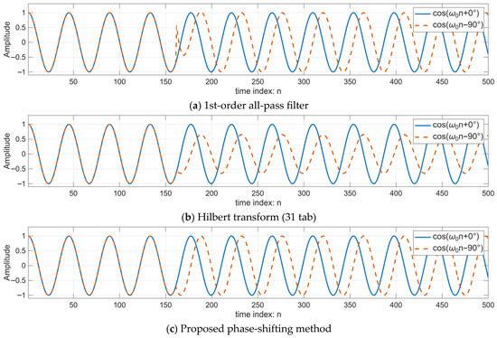
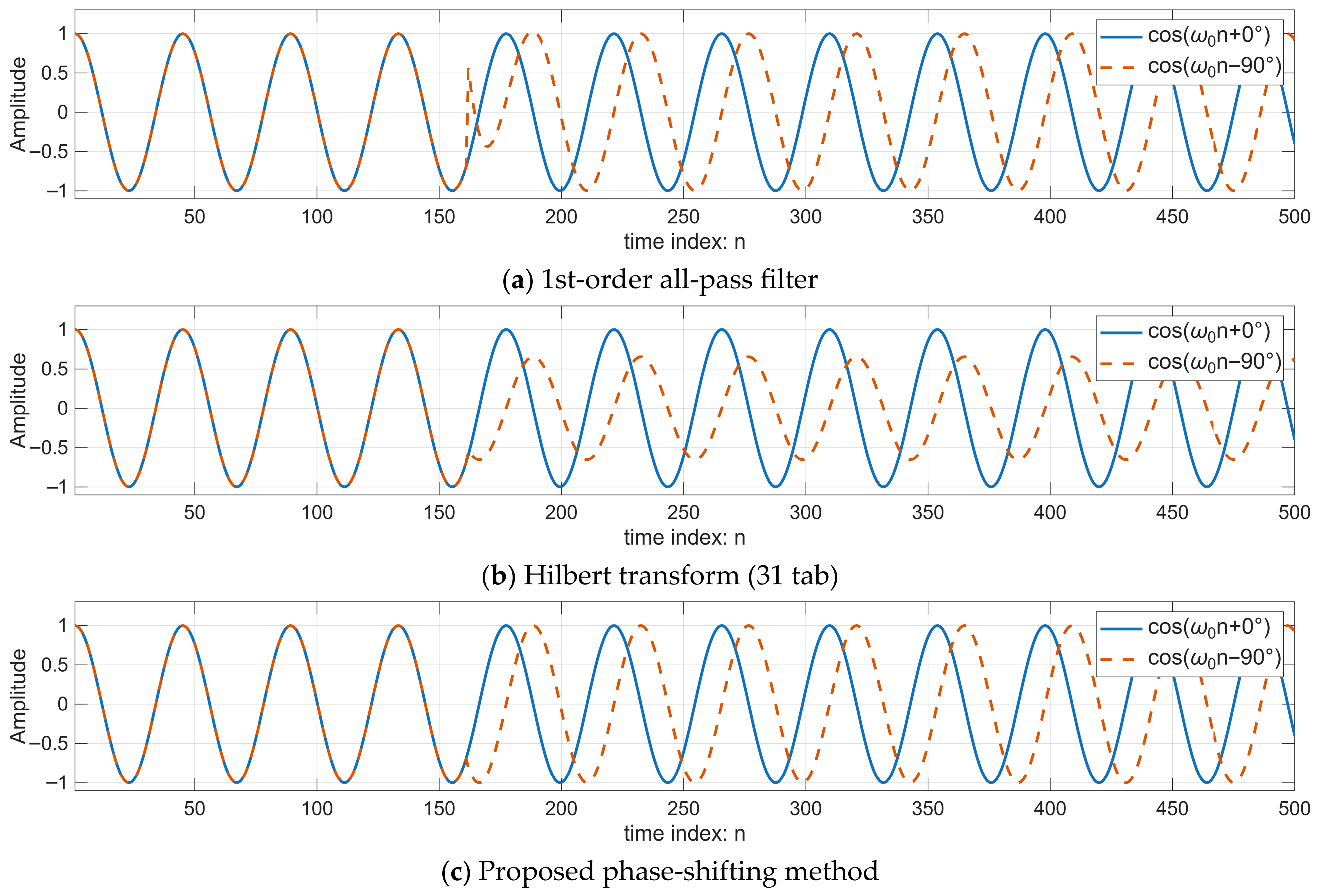
To evaluate the performance of the proposed phase-shifting method, experiments were conducted by comparing it with a first-order all-pass filter and the Hilbert transformer under the same conditions. The results are shown in Figure 20.

Figure 20. Comparison of phase adjustment from 0° to −90°.

Figure 20 illustrates a comparison of phase adjustment from 0° to −90° at n = 162 using three different methods: a first-order all-pass filter, a Hilbert transform-based approach, and the proposed method. In each plot, the solid blue line represents the reference signal, while the dashed orange line denotes the phase-shifted signal. Figure 20a presents the phase-shifting results obtained using a first-order all-pass filter. The experimental results reveal that at the onset of the phase adjustment, the signal exhibits discontinuities in both phase and amplitude. However, after a certain period, both parameters gradually converge toward their desired values and reach a stable state. This transient behavior is a characteristic limitation of the all-pass structure when coefficients are abruptly updated. In contrast, the proposed method (as shown in Figure 20c) eliminates these artifacts, providing a substantially smooth transition. Figure 20b illustrates the phase-shifting results using a 31-tap Hilbert transform, which achieves a satisfactory level of phase accuracy. However, utilizing an insufficient number of taps can lead to significant magnitude distortion. In practical applications, Hilbert filters are typically designed with a higher number of taps to ensure amplitude consistency for a wide frequency bandwidth and minimize signal distortion. Figure 20c demonstrates the phase-shifting results achieved by the proposed method. The results confirm that the system provides high phase accuracy while maintaining a constant signal amplitude, effectively eliminating any adverse effects on the output magnitude.

To provide a comprehensive performance evaluation of the phase shifter, a structural analysis of the competing methods was conducted. This analysis focuses on computational complexity, quantified by the number of multiplications and additions required, as well as the memory requirements in terms of unit-delay elements. The comparative results are summarized in Table 3.

Table 3. A comparison of the structural complexity of different phase shifting methods.

Methods	Adder	Multiplier	Unit-Delay
The cascaded first-order all-pass filter	4	4	2
The 31-tap Hilbert transform	17	17	30
Proposed phase-shifting method	2	4	1

Table 3 highlights the structural complexity of each evaluated method. The 31-tap Hilbert transform exhibits the highest complexity, requiring 17 additions, 17 multiplications, and 30 unit-delay elements, resulting in a higher implementation cost compared to the other approaches. In contrast, the cascaded first-order all-pass filter configuration—consisting of two sections—utilizes 4 additions, 4 multiplications, and 2 unit-delays. This cascaded structure is necessary because a single first-order section is phase-limited to a range of −180° to 0°, making it insufficient for full-range phase shifts from −180° to +180°. Notably, the proposed phase-shifting method demonstrates the lowest complexity among the three, requiring only 2 additions, 4 multiplications, and a single unit-delay element. This reduction in hardware resources confirms the efficiency of the proposed architecture for real-time digital signal processing applications.

4.3. Real-Time Implementation

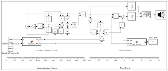
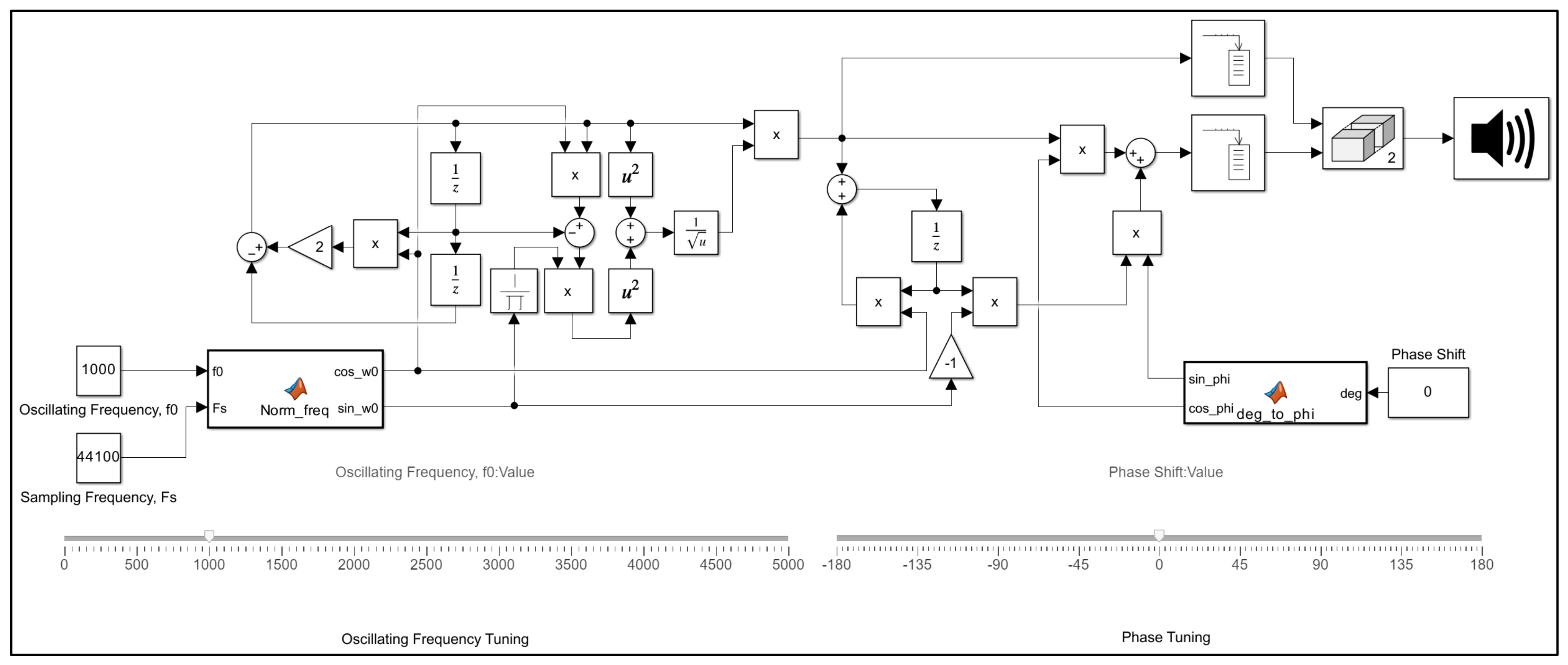
The complete architecture of the proposed continuously tunable frequency and phase biquad oscillator, as illustrated in Figure 11, was evaluated through a real-time simulation framework. This setup enables on-line adjustment of both the frequency parameter (${\omega }_0$) and the phase parameter ($\varphi$) using Simulink. To validate the system’s practical performance, the digital signals were converted through a sound card, and the resulting physical waveforms were measured and captured using an oscilloscope, as shown in Figure 21. While the system is operating, the interface of the system is designed to feature two slider controls that allow for the adjustment of the vibration frequency within the range of 0–5000 Hz and the setting of the output signal phase within the range of −180° to 180°. These controls are designed to assist the process of altering parameters during operation.

Figure 21. Simulink model for testing frequency tuning and phase control of the signal.

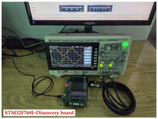
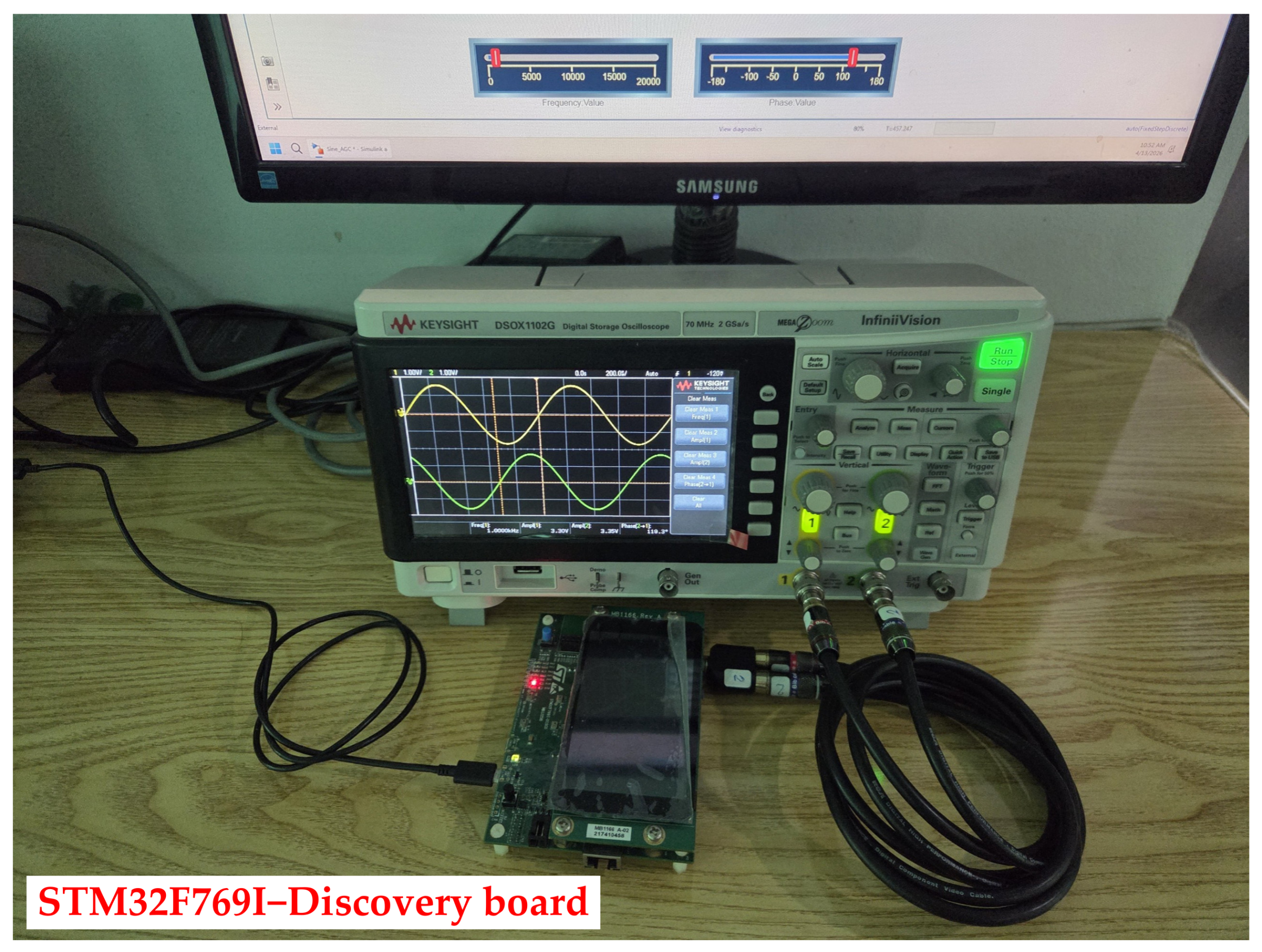
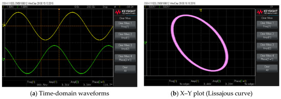
Furthermore, to validate the practical implementation of the proposed architecture, a hardware prototype was developed using the STM32F769I−Discovery board (STMicroelectronics, Geneva, Switzerland), which features an ARM Cortex−M7 32−bit RISC core-based embedded processor, as shown in Figure 22. This hardware setup facilitates the generation of oscillation signals with independent frequency and phase control directly on the embedded system. The measured waveforms captured via an oscilloscope are presented in Figure 23. Additionally, a demonstration video showcasing the real-time operation and signal measurement of the developed system is available as Video S1 in the Supplementary Materials.

Figure 22. Hardware setup for real-time processing experiment.

Figure 23. Hardware measurement results illustrating the phase difference.

5. Conclusions

The biquad oscillator has been studied and improved to enable users to dynamically adjust both the frequency and phase of the generated signal. The zero-input response analysis was employed to address the problem of amplitude instability during online frequency changes. By calculating appropriate compensation gain, the amplitude of the oscillating signal can be maintained at a constant level. In addition, a method for simplifying the computation of the inverse matrix used in the amplitude stabilization process has also been proposed in order to reduce computational complexity.

For real-time continuous phase tuning, a 1st-order IIR filter is employed, which can cover a wide phase range of [−180°, 180°]. Moreover, the tuning of the phase control parameter is independent of the input signal frequency. In contrast, a 1st-order all-pass filter cannot achieve this property. Although the phase range can be extended by cascading multiple 1st-order all-pass filters, the relationship among phase, frequency, and tuning the filter coefficients becomes complex. As a result, the phase cannot be adjusted independently without considering the relationship with the operating frequency. In addition, the Hilbert transform can provide phase adjustment over a wide range of [−180°, 180°], but its structural implementation is significantly more complex than the proposed phase tuning approach. Both simulation results and hardware experiments confirm that the modified biquad oscillator, which allows dynamic adjustment of frequency and phase, can operate effectively and provide practical benefits for users.

However, when the frequency is changed abruptly with a large step, a phase discontinuity may occur, depending on both the step size and the switching instant. This effect is caused by the immediate update of digital oscillator coefficients; specifically, the previously stored states in the unit delays do not fully match the oscillatory basis of the new frequency. This phase discontinuity is an inherent limitation of the proposed amplitude stabilization mechanism and can be viewed as a transient error, similar to the amplitude fluctuations that occur only at the instant of frequency transition. In practical operation, such as gradual frequency adjustment via a knob or slider (analog-like tuning), the frequency variation is continuous, and the phase discontinuity becomes negligible. Future work will focus on further mitigating this effect under large-step transitions and extending the proposed method toward practical applications, particularly in impedance measurement instruments.

References

- Kroupa, V.F. A new architecture for a sinewave output DDS with high spectral purity. In Direct Digital Frequency Synthesizers; IEEE: Piscataway, NJ, USA, 1999; pp. 352–357. [Google Scholar] [CrossRef] [Scilit]
- Meenakarn, C.; Thanachayanont, A. A sine-output ROM-less direct digital frequency synthesiser using a polynomial approximation. In Proceedings of the 2003 International Symposium on Circuits and Systems (ISCAS 2003), Bangkok, Thailand, 25–28 May 2003; pp. 625–628. [Google Scholar] [CrossRef] [Scilit]
- Chau, Y.A.; Chen, Y.-H. A high-performance ROM-less direct digital frequency synthesiser. AEU—Int. J. Electron. Commun. 2011, 65, 272–274. [Google Scholar] [CrossRef] [Scilit]
- Liao, X.; Zhang, L.; Hu, X.; Peng, Y.; Zhou, T. FPGA implementation of a higher SFDR upper DDFS based on non-uniform piecewise linear approximation. Appl. Sci. 2023, 13, 10819. [Google Scholar] [CrossRef] [Scilit]
- Xing, X.; Melek, W.; Wang, W. A recursive trigonometric technique for direct digital frequency synthesizer implementation. Electronics 2024, 13, 4762. [Google Scholar] [CrossRef] [Scilit]
- Turner, C.S. Recursive discrete-time sinusoidal oscillators. IEEE Signal Process. Mag. 2003, 20, 103–111. [Google Scholar] [CrossRef] [Scilit]
- Hiasat, A.A.; Al-Khateeb, A.M. New high-resolution digital sinusoidal oscillator structure with extremely low frequency and sensitivity. Int. J. Electron. 1999, 86, 287–296. [Google Scholar] [CrossRef] [Scilit]
- Dattorro, J. Effect design. Part 3: Oscillators: Sinusoidal and pseudonoise. J. Audio Eng. Soc. 2002, 50, 115–146. [Google Scholar]
- Smeets, H.; Ceriotti, M.; Marrón, P.J. Adapting recursive sinusoidal software oscillators for low-power fixed-point processors. ACM Trans. Embed. Comput. Syst. (TECS) 2020, 19, 17. [Google Scholar] [CrossRef] [Scilit] [PubMed]
- Hong, S.-K.; Jee, D.-W. A 0.052 mm2, <0.4% THD, sinusoidal current generator for bio-impedance measurement using a recursive digital oscillator and current-domain FIR filter. IEEE Trans. Circuits Syst. II Express Briefs 2019, 66, 894–898. [Google Scholar] [CrossRef]
- Chivapreecha, S.; Suwannawach, P.; Sato, T. Amplitude stabilization of frequency-tunable biquad digital oscillator using zero-input response analysis. In Proceedings of the 2024 International Conference on Photonics Solutions (ICPS 2024), Bangkok, Thailand, 9–11 December 2024. [Google Scholar] [CrossRef] [Scilit]
- Sotner, R.; Polak, L.; Jerabek, J.; Jaikla, W. Arbitrarily tunable phase shift in low-frequency multiphase oscillator. IEEE Trans. Instrum. Meas. 2023, 72, 2004711. [Google Scholar] [CrossRef] [Scilit]
- Smith, J.O. An allpass approach to digital phasing and flanging. In Proceedings of the International Computer Music Conference (ICMC), Paris, France, 19–23 October 1984. [Google Scholar]
- Kiiski, R.; Esqueda, F.; Välimäki, V. Time-variant gray-box modeling of a phaser pedal. In Proceedings of the International Conference on Digital Audio Effects (DAFx-16), Brno, Czech Republic, 5–9 September 2016; pp. 31–38. [Google Scholar]
- Duraiswamy, P.; Bauwelinck, J.; Vandewege, J. Efficient implementation of 90° phase shifter in FPGA. EURASIP J. Adv. Signal Process. 2011, 2011, 32. [Google Scholar] [CrossRef] [Scilit]
- Chivapreecha, S.; Jongsataporn, T. Tunable 1st Order IIR Phase Shifter Design and Implementation. In Proceedings of the TENCON 2024—2024 IEEE Region 10 Conference (TENCON), Singapore, 1–4 December 2024. [Google Scholar] [CrossRef] [Scilit]
- Smith, J.O., III. Introduction to Sound Processing; Stanford University: Stanford, CA, USA, 2011. [Google Scholar]
- Tierney, J.; Rader, C.; Gold, B. A digital frequency synthesizer. IEEE Trans. Audio Electroacoust. 1971, 19, 48–57. [Google Scholar] [CrossRef] [Scilit]
- Oppenheim, A.V.; Schafer, R.W. Discrete-Time Signal Processing, 3rd ed.; Pearson: Upper Saddle River, NJ, USA, 2010. [Google Scholar]
Disclaimer/Publisher’s Note: The statements, opinions and data contained in all publications are solely those of the individual author(s) and contributor(s) and not of MDPI and/or the editor(s). MDPI and/or the editor(s) disclaim responsibility for any injury to people or property resulting from any ideas, methods, instructions or products referred to in the content. |
© 2026 by the authors. Licensee MDPI, Basel, Switzerland. This article is an open access article distributed under the terms and conditions of the Creative Commons Attribution (CC BY) license.