Fault Diagnosis of Subway Traction Motor Bearings Under Variable Conditions Based on BA-VMD and SA-CNN Information Fusion

Abstract

Traditional approaches for identifying bearing defects in metro traction systems often suffer from low diagnostic efficiency and accuracy. To address this, we propose an information fusion approach using the Bat Algorithm-Optimized Variational Mode Decomposition (BA-VMD) and the Self-Attention Convolutional Neural Network (SA-CNN). Vibration and acoustic emission signals are denoised via BA-VMD to optimize decomposition, followed by a diagnosis model utilizing attention-based fusion and SA-CNN to enhance key feature extraction. Experiments on subway traction motor bearings under varying operating conditions demonstrate the method’s efficacy. Results indicate that BA-VMD achieves a signal-to-noise ratio of 6.791, which is 1.595 higher than that of EMD (5.196). Furthermore, the SA-CNN model achieves an average diagnostic accuracy of 98.6%, significantly outperforming MLP (93.57%) and SVM (90.90%). These findings confirm that the proposed framework ensures accurate and stable bearing fault detection in highly variable operating conditions.

1. Introduction

Rolling bearings are pivotal components in mechanical equipment, where their operational health determines overall system’s reliability and safety. In high-speed, heavy-load applications such as subway traction motors, bearings are subjected to complex, variable loads and speeds for extended periods, making them prone to failures caused by fatigue, wear, or localized damage. Severe failures can lead to equipment downtime or even safety accidents. Therefore, developing efficient and accurate bearing fault diagnosis methods is crucial for ensuring the safety of rail transit systems.

However, subway traction motors frequently operate under highly variable speeds and loads. This non-stationary environment generates complex noise that severely masks early fault signatures. Traditional fixed-parameter signal processing methods often fail to adapt to these changes, resulting in missed detections or false alarms. Consequently, developing an adaptive and robust diagnosis method is the primary motivation of this work.

During bearing fault diagnosis, collected vibration and acoustic emission signals frequently carry substantial background noise and interference, which may obscure weak fault features [1]. Especially in environments like subway traction motors, environmental noise, electromagnetic interference, and coupled vibration of the transmission system further reduce the signal-to-noise ratio [2]. Studies indicate that in raw signal, the energy of effective fault features may account for only 5–15% of the total signal energy [3,4,5]. Recent research by Wei et al. and Zuo et al. further highlights that under variable speed conditions, non-stationary noise significantly obscures these weak fault signatures, making feature extraction a critical challenge [4,5]. Traditional denoising methods, such as wavelet thresholding [6] and Empirical Mode Decomposition (EMD) [7], have laid the foundation for signal processing. However, recent studies [8,9] indicate that these methods face challenges such as modal aliasing and endpoint effects when processing complex non-stationary signals [10]. For instance, Zhang et al. highlighted the limitations of EMD in suppressing noise interference during early fault detection [8]. Conversely, in the fault diagnosis stage, traditional Convolutional Neural Networks (CNNs) often suffer from insensitivity to sequence length and position information [11]. Furthermore, relying on a single sensor source often leads to incomplete feature extraction. Bearing faults exhibit multiple complex modes; thus, single-sensor data cannot fully capture the essence of the fault. Therefore, developing efficient adaptive signal denoising methods and robust fault diagnosis models is crucial for enhancing detection precision.

Recent studies [12,13] have confirmed that Variational Mode Decomposition (VMD) [14] can effectively separate noise and extract data features, showing superiority over EMD [15]. VMD has been successfully applied in fields such as battery health prediction [16] and energy consumption forecasting [17]. However, VMD performance heavily depends on parameter selection, specifically the number of modes ($K$) and the penalty factor ($\alpha$). To address this, researchers have proposed various optimization strategies. For instance, Wang and Tong used the INFO algorithm [18], while Yang and Zhou employed the Slime Mold Algorithm (SMA) [19]. Zhou et al. proposed a method based on the Whale Gray Wolf Optimization algorithm [9]. Among these, the Bat Algorithm [20] has attracted attention due to its high adaptability and fast convergence. Inspired by the echolocation behavior of microbats, BA effectively balances local and global optimal solutions [21] and has been widely used in feature selection [21] and control system optimization [22]. Although BA has been combined with VMD in some studies [23,24,25], its application in optimizing VMD for subway traction motor bearings under variable conditions requires further investigation.

In the fault diagnosis stage, deep learning techniques have shown significant potential. However, traditional CNNs are often insensitive to sequence position and long-distance dependencies [10]. To overcome this, the Attention mechanism, initially proposed by Bahdanau et al. [26], helps neural networks focus on relevant information. The Self-Attention mechanism, in particular, can effectively capture intrinsic data connections [27,28,29], highlighting the correlation between vibration characteristics and acoustic emission signals. Furthermore, multi-sensor information fusion is crucial for obtaining comprehensive fault information [30,31]. By fusing vibration and acoustic emission signals, the model leverages the complementary advantage of both: the sensitivity of vibration signals to periodic impacts and the sensitivity of acoustic emission signals to early-stage micro-cracks.

Based on the analysis above, this paper proposes an information fusion fault diagnosis method based on Bat Algorithm-optimized Variational Mode Decomposition (BA-VMD) and Self-Attention Convolutional Neural Network (SA-CNN). The main contributions of this study are as follows:

Adaptive Signal Denoising Strategy: To address the issue of weak fault features being submerged by strong background noise, an improved BA-VMD method is proposed. Unlike traditional VMD with fixed parameters, this study utilizes the Bat Algorithm to adaptively optimize the decomposition parameters ($K$ and $\alpha$) by minimizing envelope entropy. This significantly enhances the Signal-to-Noise Ratio and extracts impulse features more effectively than EMD.

Novel Fault Diagnosis Model (SA-CNN): A Self-Attention Convolutional Neural Network (SA-CNN) is constructed to overcome the limitations of traditional CNNs, which are often insensitive to sequence position and long-distance dependencies. By embedding a self-attention mechanism, the model dynamically assigns higher weights to critical fault features while suppressing irrelevant noise, thereby improving diagnostic accuracy under variable operating conditions.

Multi-source Information Fusion Framework: A feature-level fusion strategy integrating Vibration and Acoustic Emission signals is developed. This approach leverages the complementary advantages of both sensors—vibration sensitivity to periodic impacts and acoustic emission sensitivity to early-stage micro-cracks—ensuring robust and stable fault detection compared to single-sensor methods.

Comprehensive Experimental Validation: A dedicated subway traction motor bearing test bench is built to simulate realistic variable working conditions (variable speeds and loads). Extensive experiments demonstrate that the proposed method achieves a diagnostic accuracy of 98.60%, significantly outperforming traditional methods like MLP and SVM, and validating its effectiveness in complex industrial scenarios.

In summary, to address the difficulties in extracting bearing fault features, the limitations of single input signals, and low fault recognition rates, this paper proposes a bearing fault diagnosis method based on BA-VMD signal denoising and SA-CNN information fusion. First, NU216 subway traction motor bearings serve as the experimental subject; bearing faults are artificially induced, and a variable working condition test bench is built to collect vibration and acoustic emission signals. Second, the BA-VMD method effectively eliminates noise from raw signals; finally, the study constructs a bearing fault detection framework using SA-CNN and information fusion, feeding the denoised signals into the model for fault diagnosis.

2. Proposed Methodology

2.1. Overall Framework

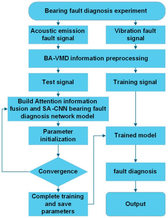
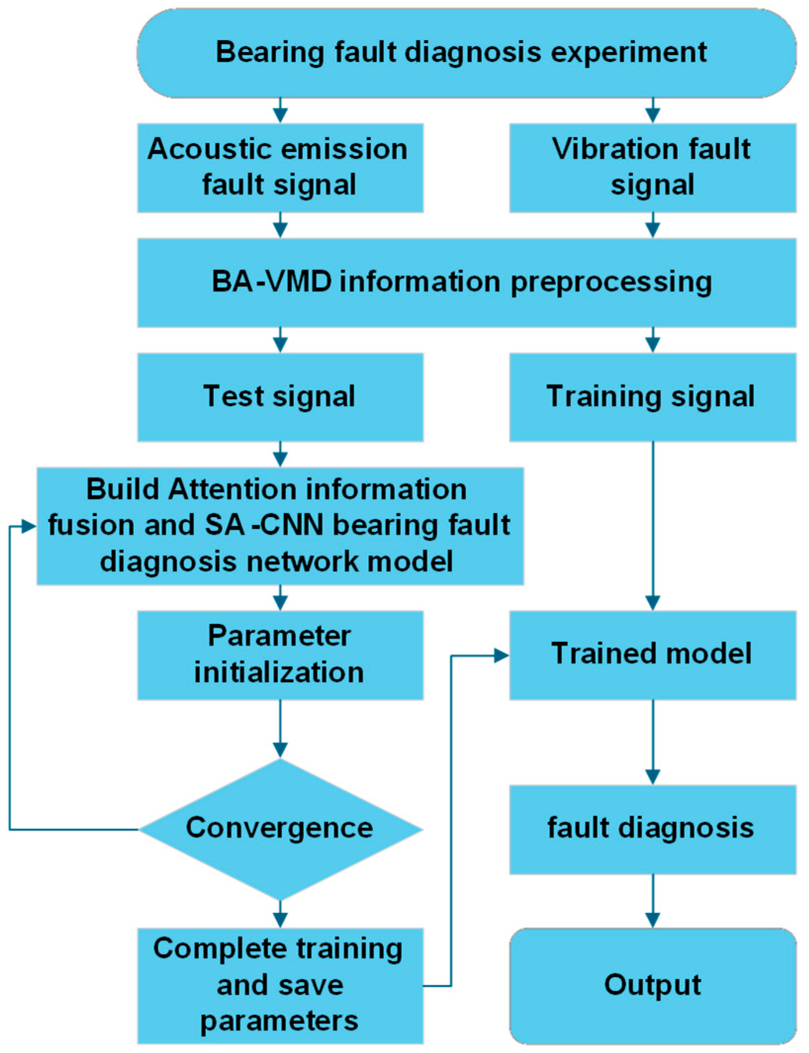
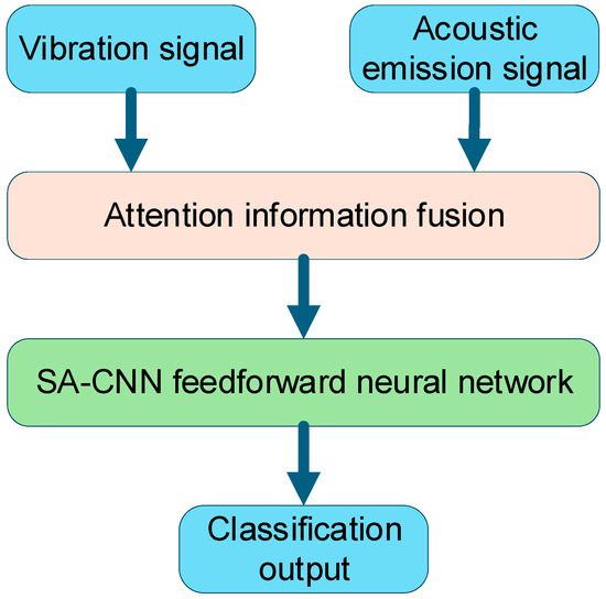
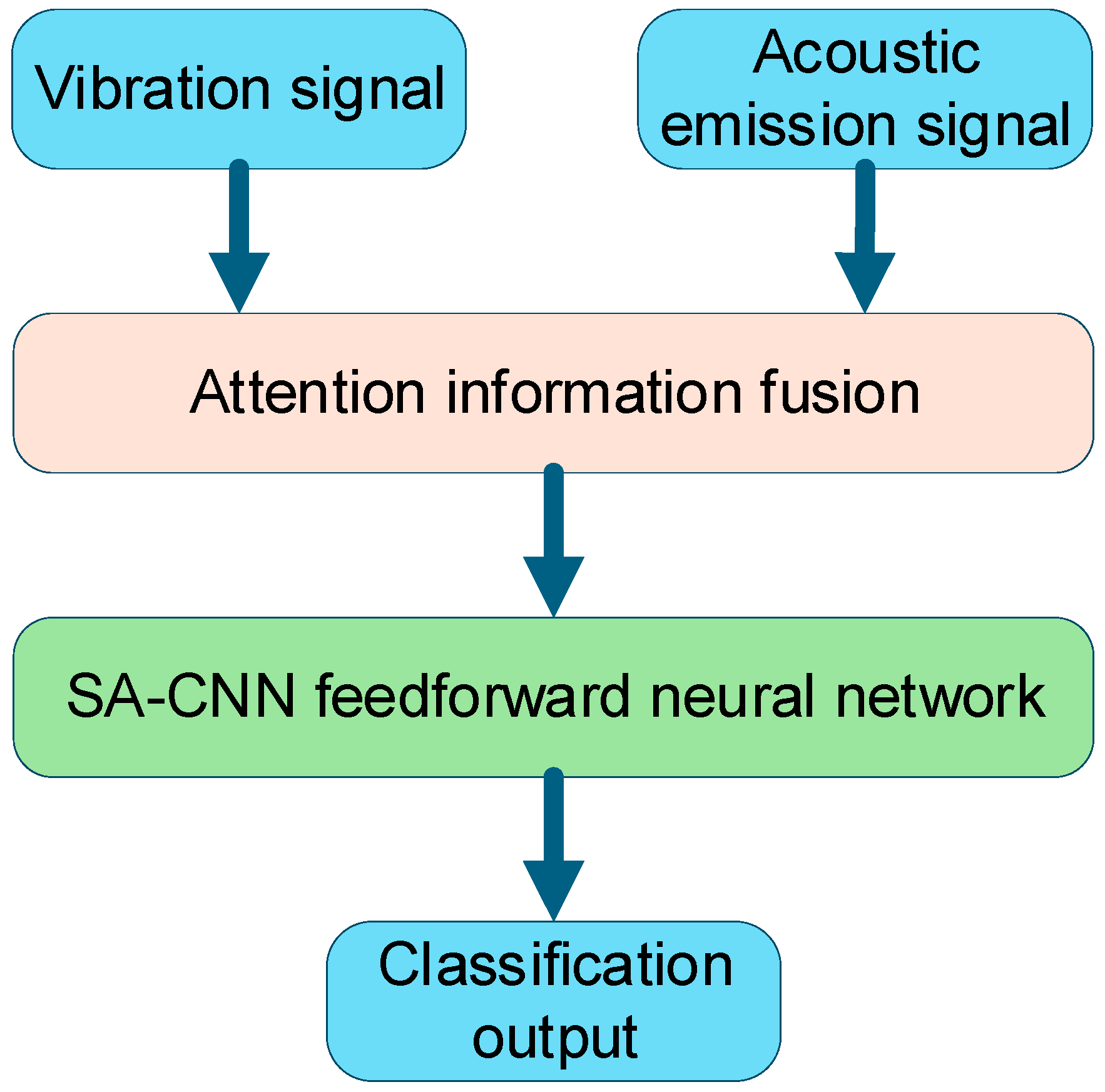
This study proposes a bearing fault diagnosis framework for subway traction motors based on multi-source information fusion. As illustrated in Figure 1, the methodology encompasses three core stages:

Figure 1. Fault diagnosis process of metro traction motor bearings.

• Signal acquisition: Vibration and Acoustic Emission signals are collected under variable operating conditions.
• Signal preprocessing: The BA-VMD is utilized to denoise raw signals and extract fault features adaptively.
• Fault diagnosis: The SA-CNN is constructed to fuse multi-source information and identify fault patterns.

To ensure robustness, an adaptive parameter selection strategy is employed. The VMD parameters ($K$ and $\alpha$) are determined by the Bat Algorithm by minimizing envelope entropy, avoiding the subjectivity of manual selection. The hyperparameters of the BA (population size and iteration number) are set to 20 and 50, respectively, to balance computational efficiency and global optimization capability.

2.2. Signal Denoising Based on BA-VMD

2.2.1. Theoretical Foundation

To address noise interference, this study employs VMD for signal decomposition. VMD is a non-recursive algorithm that adaptively decomposes the original signal into multiple Intrinsic Mode Functions (IMFs) by minimizing the sum of their estimated bandwidths [14]. Unlike Empirical Mode Decomposition (EMD), VMD has a solid theoretical foundation and effectively mitigates modal aliasing. The constrained variational problem is formulated as Equation (1):

$$\left\{\begin{array}{c}\underset{\left\{u_k\right\},\left\{{\omega }_k\right\}}{\min }\left\{{\displaystyle \sum _{k=1}^K}{‖{\mathsf{\partial }}_t\left[\left(\delta \left(t\right)+{\displaystyle \frac{j}{\pi t}}\right)u_k\left(t\right)\right]e^{-j{\omega }_{k}t}‖}_2^2\right\}\\ s.t.{\displaystyle \sum _{k=1}^K}{u}_k=f\end{array}\right.,$$

(1)

where $\left\{u_k\right\}$ is each modal function, $\left\{u_k\right\}=\left\{u_1,u_2,\dots ,u_k\right\}$; $\left\{{\omega }_k\right\}$ is the center frequency of each modal function, $\left\{{\omega }_k\right\}=\left\{{\omega }_1,{\omega }_2,\dots ,{\omega }_k\right\}$. $K$ is the number of modal component functions, and $\delta \left(t\right)$ is the Dirac distribution.

The quadratic penalty factor α and the Lagrangian multiplication operator λ(t) are introduced to transform the constrained variational problem into an unconstrained variational problem. The quadratic penalty factor α can ensure the accuracy of signal reconstruction, and the Lagrangian multiplication operator λ(t) can ensure the strictness of the constraints. The extended Lagrangian expression Equation (2) is as follows:

$$\begin{array}{ll}L\left(u_k,{\omega }_k,\lambda \right)& =\alpha {\displaystyle \sum _{k=1}^K}{‖{\mathsf{\partial }}_t\left[\left(\delta \left(t\right)+{\displaystyle \frac{j}{\pi t}}\right)u_k\left(t\right)\right]e^{-j{\omega }_{k}t}‖}_2^2+{‖f-{\displaystyle \sum _k}{u}_k\left(t\right)‖}_2^2\\ & +⟨\lambda \left(t\right),f\left(t\right)-{\displaystyle \sum _k}{u}_k\left(t\right)⟩.\end{array}$$

(2)

The alternating direction multiplier method is used to alternately update ${\widehat{u}}_k^{n+1},{ \omega }_k^{n+1}, {\lambda }^{n+1}$ to locate the saddle point in the augmented Lagrangian formulation. The expression Equation (3) for updating the modal component is:

$${\widehat{u}}_k^{n+1}\left(\omega \right)={\displaystyle \frac{\widehat{f}\left(\omega \right)-\sum _{i\ne k}{\widehat{u}}_i\left(\omega \right)+\frac{\widehat{\lambda }\left(\omega \right)}{2}}{1+2\alpha {\left(\omega +{\omega }_k\right)}^2}}.$$

(3)

The expression Equation (4) for updating the center frequency of the modal component is:

$${\omega }_k^{n+1}={\displaystyle \frac{{{\int }_0^{\infty }\omega \left|{\widehat{u}}_k\left(\omega \right)\right|}^{2}d\omega }{{{\int }_0^{\infty }\left|{\widehat{u}}_k\left(\omega \right)\right|}^{2}d\omega }}.$$

(4)

The expression Equation (5) of the updated Lagrange multiplication operator is:

$${\lambda }^{n+1}={\lambda }^n+\tau \left(f-\sum _k{\widehat{u}}_k^{n+1}\right).$$

(5)

To optimize the parameters $K$ (number of modes) and $\alpha$ (penalty factor) in VMD, the Bat Algorithm (BA) is utilized. Inspired by the echolocation behavior of microbats, BA simulates the bats’ movement in a D-dimensional search space [22]. The position $x_i$ and velocity $v_i$ of the $i$-th bat are updated according to Equations (6) and (7):

$$v_i^{t+1}=v_i^t+(x_i^t-x_{best})\cdot f_i,$$

(6)

$$x_i^{t+1}=x_i^t+v_i^{t+1}.$$

(7)

where $f_i$ is the frequency, calculated as Equation (8):

$$f_i=f_{min}+(f_{max}-f_{min})\cdot \beta .$$

(8)

Here, $\beta$ is a random vector, and $x_{best}$ represents the current global best solution. BA balances local and global search through frequency tuning and pulse emission mechanisms.

However, VMD performance heavily depends on the number of modes ($K$) and the penalty factor ($\alpha$). To optimize these parameters, the Bat Algorithm is utilized. Inspired by the echolocation behavior of microbats, BA simulates the movement of bats in a D-dimensional search space to find the global optimum [20]. It balances local and global searches through frequency tuning and pulse emission mechanisms, making it suitable for optimizing the non-linear parameters of VMD.

2.2.2. Improved BA-VMD Denoising Strategy

To enhance the denoising efficiency, this paper introduces an improved fitness function and a screening mechanism.

Fitness Function Selection: Conventional methods often rely on subjective parameter selection. In this study, Envelope Entropy is selected as the fitness function to guide the bat algorithm in searching for the optimal solution. When a localized defect occurs, the bearing generates periodic impulses that introduce a high degree of order and sparsity in the signal’s envelope.

Mathematically, envelope entropy quantifies this complexity: a lower entropy value corresponds to a signal with stronger periodicity (characteristic of fault impulses), while a higher entropy value indicates randomness (characteristic of noise). Therefore, minimizing envelope entropy effectively guides the BA-VMD to extract impulse components most relevant to the fault.

The envelope entropy $E$ is calculated as follows:

$$E(x)=-{\sum }_{i=1}^N{p}_i\mathrm{l}\mathrm{n}{p}_i.$$

(9)

where $p_i$ is the normalized envelope signal. The objective is to minimize the sum of the modal component envelope entropies, as lower entropy indicates stronger fault characteristics and less noise.

Screening Function Selection: After decomposition, not all IMFs are useful. The Pearson Correlation Coefficient is employed to measure the correlation between each modal component $u_k$ and the original signal $f$. The coefficient $R$ is defined as Equation (10):

$$R={\displaystyle \frac{\mathit{Cov}(u_k,f)}{{\sigma }_{u_k}{\sigma }_f}},$$

(10)

Modal components with a correlation coefficient greater than a threshold (0.27 in this study) are retained, while those with weak correlation (high noise content) are discarded.

2.2.3. Signal Processing Flow

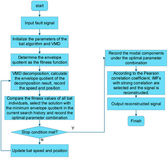
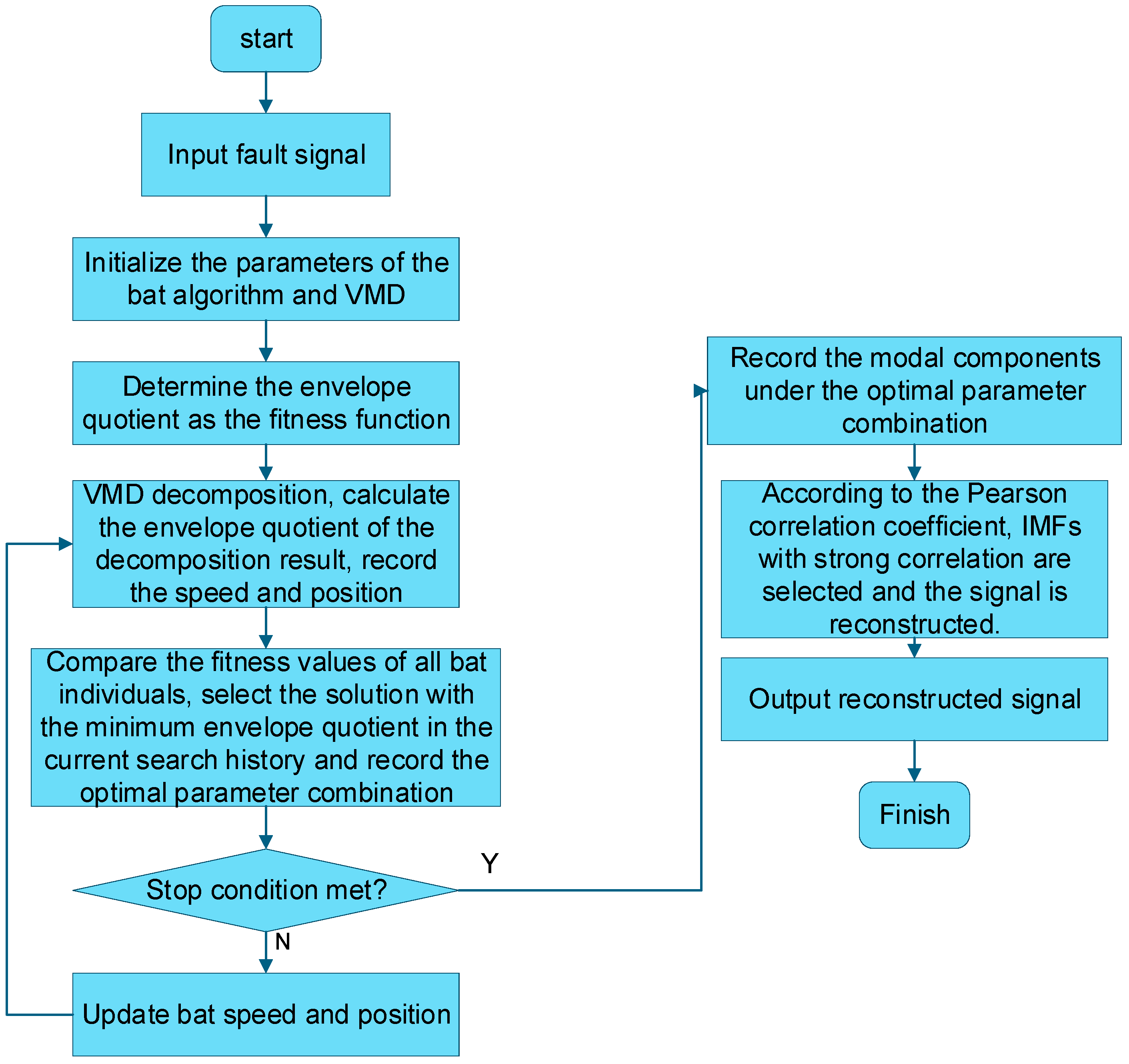
The specific flow of the proposed BA-VMD method is shown in Figure 2. The process involves:

Figure 2. Bat algorithm optimization variational mode decomposition process.

• Initialization: Initialize the bat algorithm parameters (population size, iterations) and VMD parameters ranges.
• Optimization: Utilize the bat algorithm with Envelope Entropy as the fitness function to search for the optimal parameter combination $[K,\alpha ]$.
• Decomposition And Reconstruction: Perform VMD using the optimal parameters and reconstruct the signal using IMFs with high Pearson correlation coefficients.

This approach effectively overcomes the modal aliasing problem of traditional EMD and significantly improves the Signal-to-Noise Ratio.

2.3. Fault Diagnosis Model Based on SA-CNN

2.3.1. The Self-Attention Mechanism

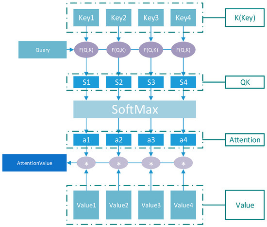
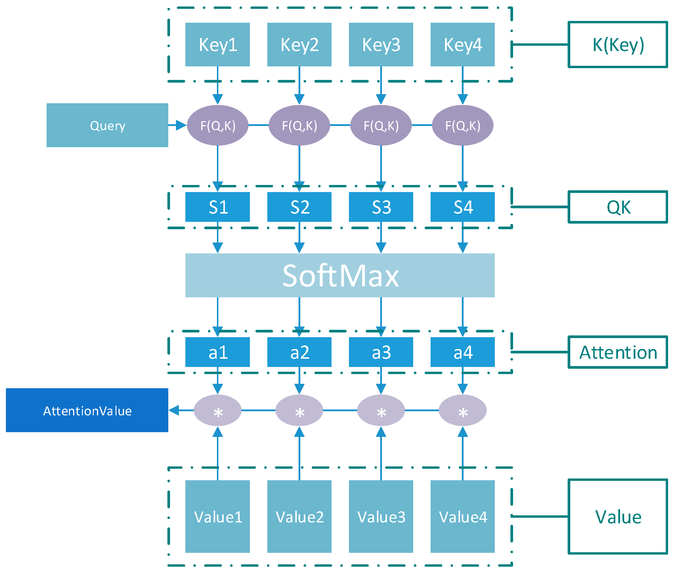
The attention mechanism allocates attention weights to Value by mapping the correlation between Query and Key [26]. The structure of the attention mechanism is shown in Figure 3.

Figure 3. Structure of the Attention Mechanism.

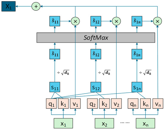
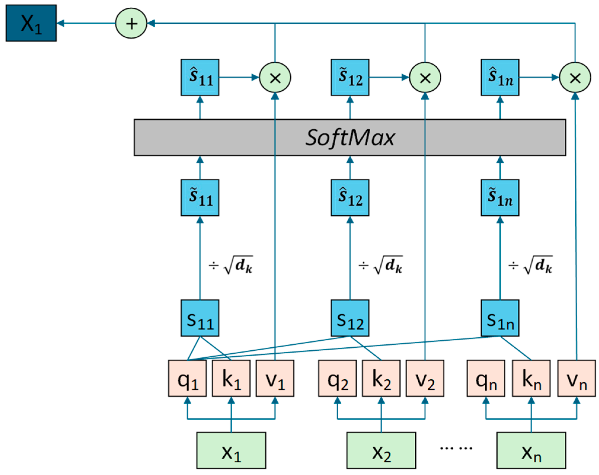
The operation process of the self-attention mechanism is as follows:

• Get Query, Key and Value. For each input vector X, multiply it by three coefficients $W^q,W^k,W^v$ to get the values of Query, Key and Value. The three Ws are parameters learned by the feedforward neural network.
• Calculate the autocorrelation of the input vector. Use the obtained Query and Key to calculate the autocorrelation of each input vector. This experiment uses the dot product operation method to calculate the autocorrelation of the input vector.
• Get the weight coefficient. Use $\sqrt{d_k}$ to control the size of the self-attention score dimension and normalize it.
• Get the output vector. Multiply the weight matrix by Value to get the output vector of the self-attention mechanism. The overall expression of the self-attention mechanism is as shown in Equation (11):

  $$z_i={\displaystyle \frac{{\mathit{e}}^{{\mathit{q}}_{\mathit{i}}^{\mathit{T}}{\mathit{k}}_{\mathit{i}}}{\mathit{v}}_{\mathit{i}}}{{\sum }_{\mathit{i}=\mathbf{1}}^{{\mathit{L}}_{\mathit{x}}}{\mathit{e}}^{{\mathit{q}}_{\mathit{i}}^{\mathit{T}}{\mathit{k}}_{\mathit{i}}}\sqrt{{\mathit{d}}_{\mathit{k}}}}},$$

  (11)

  where $i\in \left\{\mathrm{1,2},3,\dots ,n\right\}$, $z_i$ represents the output vector of the self-attention mechanism.

Figure 4 shows a diagram of the calculation process of the self-attention mechanism. where $\sqrt{d_k}$ is a parameter used to scale the dot product result, where $d_k$ represents the dimension of the key.

Figure 4. Schematic of the self-attention mechanism.

2.3.2. Network Architecture and Information Fusion

This study constructs a bearing fault diagnosis model based on Attention information fusion and SA-CNN, as shown in Figure 5.

Figure 5. Fault diagnosis model based on Attention information fusion and SA-CNN.

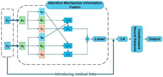
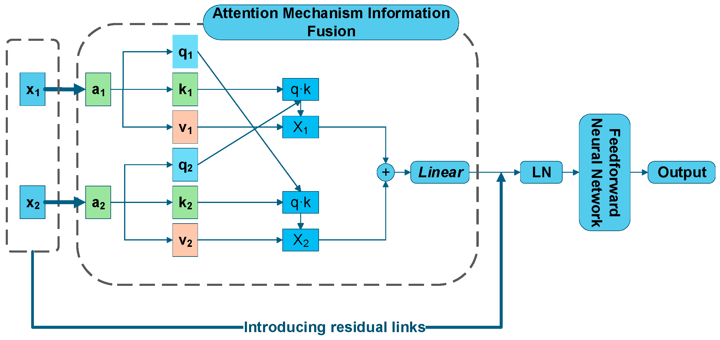
Information Fusion Strategy: As depicted in Figure 6, the vibration signal and acoustic emission signal are used as dual inputs. The Attention mechanism calculates the correlation between these two signals, dynamically allocating weights to the fault features. This fusion process combines the advantages of both sensors: the vibration signal’s sensitivity to periodic impacts and the acoustic emission signal’s sensitivity to early-stage micro-cracks. The fusion weights are dynamically learned during the network training process via backpropagation.

Figure 6. Attention mechanism information fusion structure.

It is worth noting that the fusion weights are not pre-defined constants. Instead, they are dynamically learned during the network training process. Through iterative optimization (backpropagation), the network automatically adjusts the parameters to assign appropriate weights to the acoustic emission and vibration features based on their contribution to the fault diagnosis task.

SA-CNN Structure: The detailed network architecture is shown in Figure 7. The model consists of four convolutional layers and four pooling layers for feature extraction. Specifically, a Self-Attention module is inserted after the second pooling layer. The placement of this module is strategically designed based on the trade-off between feature abstraction and spatial resolution:

Figure 7. Structure of SA-CNN.

Noise Robustness: Placing the module after the first pooling layer may lead to attention being allocated to high-frequency noise. The first two convolutional blocks act as non-linear filters, enhancing the Signal-to-Noise Ratio of the feature maps before the attention calculation.

Spatial Information Retention: Placing the module deeper (e.g., after the 3rd or 4th layer) would result in excessive downsampling, leading to the loss of fine-grained spatial details critical for identifying localized bearing faults.

Computational Efficiency: The feature map size at the 2nd pooling layer offers an optimal balance, minimizing computational cost while retaining sufficient resolution.

The architecture proceeds as follows:

• The fused signal undergoes the first two Conv-Pooling blocks.
• The Self-Attention layer strengthens the fault feature signals and suppresses irrelevant information.
• The remaining two Conv-Pooling blocks further extract high-level features.
• Finally, a Fully Connected (FC) layer maps the features to the output classes.

3. Experimental Setup

3.1. Subway Traction Motor Bearing Test Platform

To validate the effectiveness of the proposed methodology under realistic industrial scenarios, a dedicated test bench for subway traction motor bearing was established. This platform allows for the simulation of actual operating conditions and the acquisition of fault signals.

3.1.1. Experimental Bearings

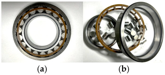
The experimental subject is the NU216 signal-row cylindrical roller bearing, widely used in subway traction motors due to its high rigidity and ability to withstand heavy bidirectional axial loads. As shown in Figure 8, the NU216 bearing consists of an inner ring, an outer ring, a cage, and cylindrical rolling elements. It features a separable design where the outer ring has integral flanges on both sides, while the inner ring is flangeless, allowing for bidirectional axial displacement.

Figure 8. Structure of NU216 bearing: (a) Overall structure; (b) Separation structure.

The dimensions and specifications of the NU216 bearings comply with the national standard GB/T 283-2021 [32]. Detailed parameters are listed in Table 1.

Table 1. NU216 bearing size specification.

NU216	Parameter
Inner diameter	80 mm
Outer diameter	140 mm
Width	26 mm
Number of rolling elements	18
Cage	Non-metal
Basic dynamic load rating	132 kN
Speed limit	3800 r/min

3.1.2. Experimental Platform

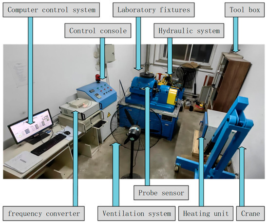
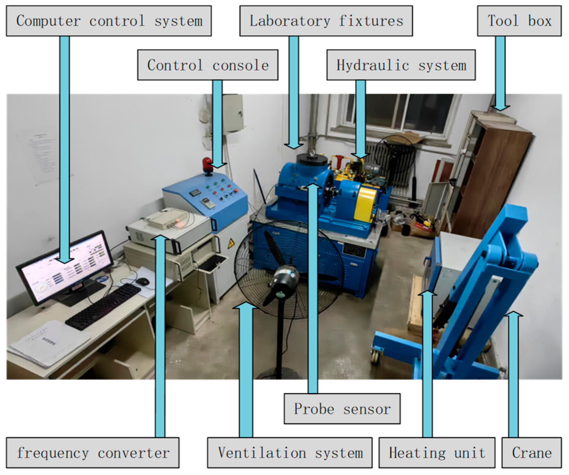
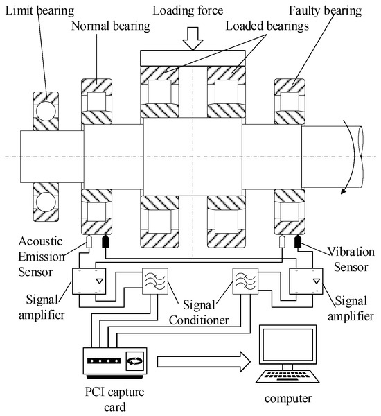
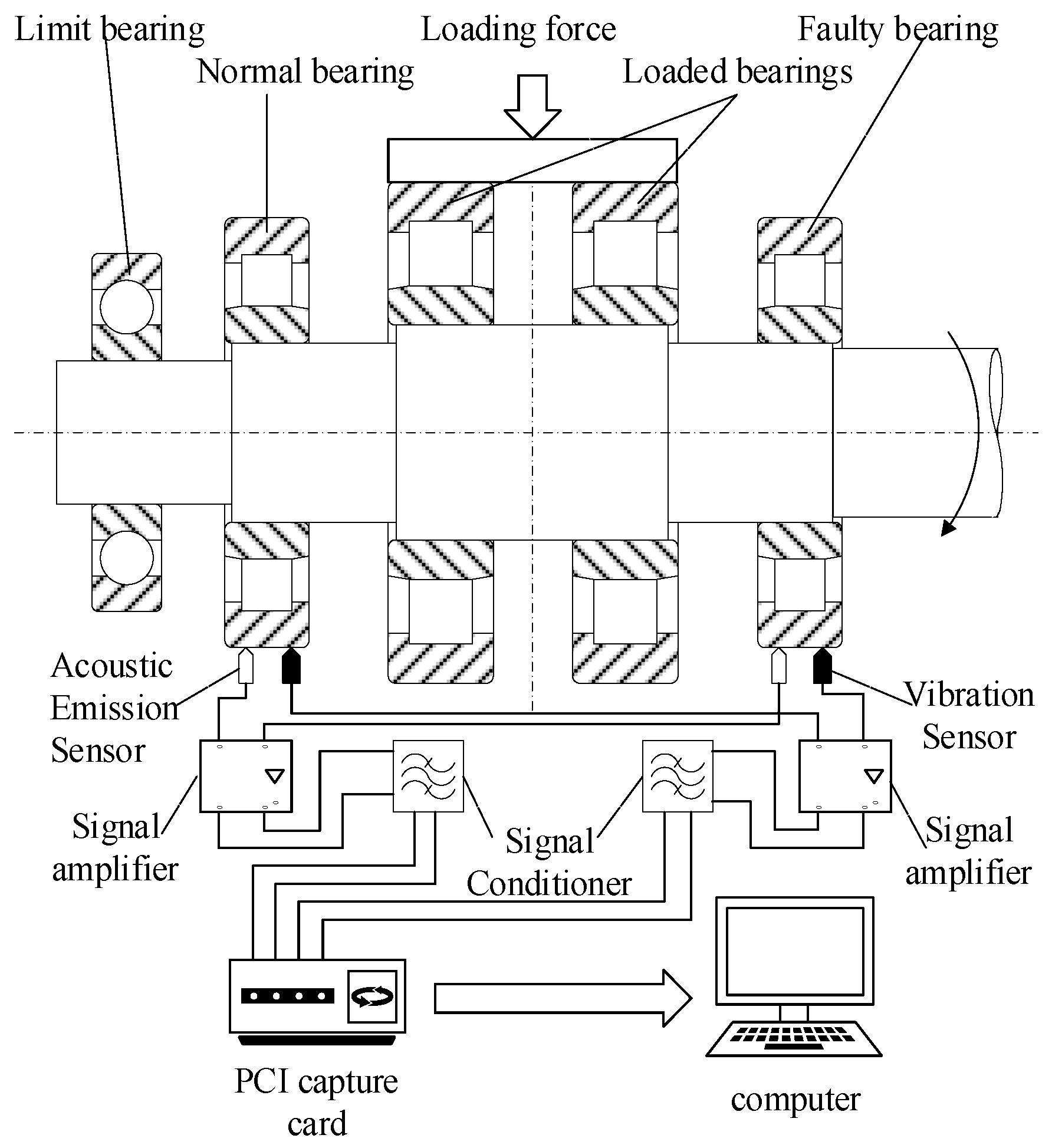
The test rig, jointly developed by the Henan Engineering Laboratory for Intelligent CNC Equipment and the Luoyang Bearing Research Institute, is illustrated in Figure 9. The system comprises a variable speed test machine, a hydraulic loading system, an information acquisition system, and a computer control unit.

Figure 9. Experimental platform for rolling bearings.

The shaft system incorporates three types of bearings: limit bearings, test bearings, and loading bearings (parameters detailed in Table 2). The loading bearings withstand the applied experimental loads, which are transmitted to the main shaft and evenly distributed to the test bearings. The limit bearings constrain axial movement caused by vibration.

Table 2. Rated Load and Limit Speed Parameters of Bearings in the Test Rig.

Bearing Parameters		Limit Bearing (6213)	Experimental Bearings (NU216)	Loaded Bearings (NU218)
Basic load rating (kN)	Dynamic load	57.2	132.0	172.0
	Static load	40.0	165.0	215.0
Speed limit (r/min)	Grease lubrication	5000	3800	3400
	Oil lubrication	6300	4800	4300

The information acquisition system includes an R50S-TC acoustic emission sensor, an LC0151T vibration accelerometer, a signal amplifier, an LC0201-5 signal conditioner, an Altai PCI8510 vibration acquisition card, and a PCI-2 acoustic emission acquisition card. The main parameters of the vibration and acoustic emission sensors are shown in Table 3 and Table 4. The parameters of the PCI8510 vibration acquisition card and PCI-2 acoustic emission acquisition card are shown in Table 5 and Table 6.

Table 3. Main parameters of vibration signal sensor.

Project	Parameter
Model	LC0151T
Range	33 g
Frequency range	0.7–13 kHz
Sensitivity	150 mV/g
Resolution	0.0002 g
Resonant frequency	50 kHz

Table 4. Main parameters of acoustic emission sensor.

Project	Parameter
Model	R50S-T
Signal output type	Voltage
Measuring range	50–700 kHz
Interface Type	BNC connector
Resonant frequency	50 kHz

Table 5. Main parameters of PCI8510 vibration signal acquisition card.

Project	Parameter
Bus interface	32-bit PCI bus
Analog input	2-channel differential input
A/D conversion	16-bithigh-precision ADC
Maximum sampling rate	500 kSPS per channel
Input range	±5 V, ±10 V (software adjustable)
Input coupling	AC/DC optional

Table 6. Main parameters of PCI-2 acoustic emission signal acquisition card.

Project	Parameter
Bus interface	32-bit PCI bus
Analog input	2-channel differential input
A/D conversion	18-bithigh-precision ADC
Maximum sampling rate	20 MSPS, 40 MSPS
Input range	±5 V, ±10 V (software adjustable)
Input coupling	AC/DC optional

In this experiment, the computer control system issues commands for variable operating conditions and data acquisition. It regulates the hydraulic loading system to apply force to the loading bearing, which is then transmitted to the main shaft and evenly distributed to the experimental bearings, thereby achieving variable load conditions. Simultaneously, the system controls a frequency converter to adjust the motor speed, which modulates the spindle rotation speed via a coupling to realize variable speed conditions.

Vibration and acoustic emission signals are captured by their respective sensors and subsequently processed by a signal amplifier and conditioner before being digitized by the corresponding acquisition cards. The schematic diagram of the bearing experimental platform is shown in Figure 10.

Figure 10. Schematic diagram of experimental platform.

Although the signal acquisition system is capable of monitoring two experimental bearings simultaneously, using two faulty bearings at once would cause signal interference and distortion. Therefore, this experiment employs a configuration of one healthy bearing and one faulty bearing to minimize experimental error. Specific parameters of the bearing experimental platform are detailed in Table 7.

Table 7. Main parameters of bearing test stand.

Project	Parameter Range
Permissible range of inner diameter of test bench shaft system	Φ40–Φ120 mm
Maximum allowable speed of the shaft system	0–3800 r/min
Maximum allowable load on the shaft	0–165 kN
Lubricating	Grease lubrication
Couplings	Flexible connection
Number of experimental bearings	7 sets
Temperature alarm	100 °C
Ventilation capacity	15,000 m3/h

3.2. Metro Traction Motor Bearing Data Collection Experiment

3.2.1. Experimental Plan

Bearing failures in rotating machinery are predominantly characterized by pitting and cracking [3,31]. Consequently, this study focuses on six major failure modes: outer ring pitting, outer ring cracking, inner ring pitting, inner ring cracking, rolling element pitting, and rolling element cracking.

To ensure data reliability and simulate actual subway operating conditions, multiple load and speed levels were established. According to safety regulations for subway traction motors, the bearing load should be maintained below 28–30% of the ultimate load, and the speed between 50% and 60% of the limit speed. Considering the constraints of the shaft system components, the maximum experimental speed was set to 2400 rpm and the maximum load to 9 kN.

The experimental loads were set at 5 kN, 7 kN, and 9 kN (fluctuating by approximately one-quarter of the maximum load), and speeds were set at 800 rpm, 1600 rpm, and 2400 rpm. The experiment covers seven bearing health states (six fault types plus one normal state) under nine operating conditions, resulting in a total of 63 sub-experiments. The experimental schedule is detailed in Table 8, and the fault label definitions are provided in Table 9.

Table 8. Experimental schedule.

Load kN	Speed r/min
	Inner Ring Pitting	Inner Ring Crack	Outer Ring Pitting	Outer Ring Crack	Rolling Element Pitting	Rolling Element Crack	Normal
5 kN	800	800	800	800	800	800	800
	1600	1600	1600	1600	1600	1600	1600
	2400	2400	2400	2400	2400	2400	2400
7 kN	800	800	800	800	800	800	800
	1600	1600	1600	1600	1600	1600	1600
	2400	2400	2400	2400	2400	2400	2400
9 kN	800	800	800	800	800	800	800
	1600	1600	1600	1600	1600	1600	1600
	2400	2400	2400	2400	2400	2400	2400

Table 9. Definition of fault labels.

Label ID	Fault Location	Fault Type
0	-	Normal
1	Rolling Element	Pitting
2	Inner Ring	Pitting
3	Outer Ring	Pitting
4	Rolling Element	Crack
5	Inner Ring	Crack
6	Outer Ring	Crack

3.2.2. Bearing Defect Fabrication

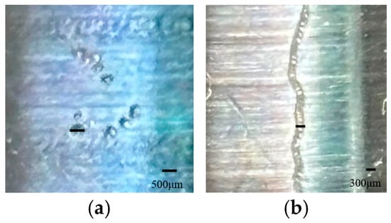
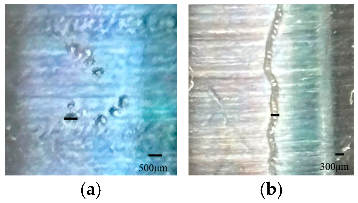
Since retired bearings often lack distinct defects due to conservative safety factors in manufacturing, artificial defects were introduced to simulate incipient faults. Pitting and crack faults were machined using an engraving machine.

Pitting faults: Fabricated with a diameter of approximately 500 μm to simulate microscopic surface damage typical of early-stage failures [33].

Crack faults: Fabricated with a width of approximately 300 μm. This dimension aligns with the range of artificial defects (178–533 μm) used in benchmark studies, such as the Case Western Reserve University (CWRU) bearing data center, ensuring the comparability of the results [3].

The specific fault morphologies are shown in Figure 11.

Figure 11. Pitting and cracking faults; (a) Pitting fault; (b) Crack fault.

3.2.3. Experimental Process

Data collection involved a pre-test phase and a formal experiment phase. The pre-test (6 min) stabilized the bearing conditions. In the formal experiment, each of the 63 sub-experiments ran for 20 min. Data were sampled four times for 10 s each, with 5 min intervals between samples. A 30 s adjustment period was allocated between condition transitions. The timing schedule is shown in Table 10.

Table 10. Test schedule.

Experiment Type	Step	Speed r/min	Load kN	Runtime s
Preliminary experiment	1	300	1	120
	2	600	3	120
	3	800	5	120
Formal experiment	1	800	5	1200 + 60 (adjustment)
	2	800	7	1200 + 60 (adjustment)
	3	800	9	1200 + 60 (adjustment)
	4	1600	5	1200 + 60 (adjustment)
	5	1600	7	1200 + 60 (adjustment)
	6	1600	9	1200 + 60 (adjustment)
	7	2400	5	1200 + 60 (adjustment)
	8	2400	7	1200 + 60 (adjustment)
	9	2400	9	1200 + 60 (adjustment)

Referencing the pre-experimental signal distribution, set the vibration sensor range to −1000 mV to 1000 mV, the sampling frequency to 50 kHz, the gain to 1, and save the data in PCI format. This data will then be processed externally to create a TXT file. Set the acoustic emission sensor range to −0.5 mV to 0.5 mV, the sampling frequency to 50 kHz, and save the data in DTA format.

It is worth noting that although the R50S-TC sensor has a resonant frequency of 50 kHz and a wide measurement range, the bearing fault signals under low-speed operating conditions (800–2400 r/min) contain significant low-frequency components (<25 kHz) that are sensitive to incipient faults. To prevent aliasing and ensure signal fidelity within the effective bandwidth, the acquisition system (incorporating the PCI-2 card and signal conditioning) acts as an anti-aliasing filter, effectively capturing the fault features within the 0–25 kHz range. Therefore, a sampling frequency of 50 kHz is sufficient to satisfy the Nyquist-Shannon sampling theorem for the frequency band of interest in this study. This data will then be processed externally to create a TXT file.

3.2.4. Data Preprocessing and Sample Augmentation

To ensure model robustness and address data volume limitations, a comprehensive preprocessing pipeline was implemented:

• Baseline Drift Removal

Affected by sensor zero drift and environmental low-frequency interference, raw signals often contain non-stationary DC components or slowly varying trend terms, which can mask weak fault impulse features. Therefore, detrending processing is first applied to the raw time-series signal $x\left(t\right)$:

$$x_{clean}\left(t\right)=x\left(t\right)-\overline{x}-trend\left(t\right),$$

(12)

where $\overline{x}$ denotes the signal mean, and $trend\left(t\right)$ represents the linear trend term fitted via the Least Squares Method. This step effectively eliminates baseline drift and highlights the AC fluctuation features of the signal.

2.

Overlapping Segmentation Strategy

The raw signals collected under each operating condition constitute continuous time-series data. Directly segmenting these signals using a fixed window length would yield a limited number of samples (approximately 122 per condition for 2 × 10⁶ data points), which is insufficient for training deep neural networks and prone to overfitting.

To augment the dataset and enhance the model’s generalization capability, a sliding window technique with a specific stride was employed. The window length was set to 16,384 data points to align with the network input requirements, and the sliding stride was set to 3975 points. This strategy effectively expanded the dataset; by shifting the window across the raw signal, the sample size was increased to 500 samples per operating condition (400 for training and 100 for testing), thereby ensuring statistical significance.

To prevent data leakage and ensure a fair evaluation, a time-series split strategy was adopted. After applying sliding window segmentation to the continuous raw signal (treated as a single acquisition), samples were partitioned sequentially. The first 80% (400 samples) were assigned to the training set, and the final 20% (100 samples) were used for testing. This strict temporal separation ensures that overlapping windows from the same acquisition do not coexist in the training and testing sets, forcing the model to generalize rather than memorize local signal patterns.

3.

Data Transformation (Tiling Method)

Since the proposed SA-CNN model requires 2D images as input, a tiling method was utilized to convert the 1D time-series signals into a 2D format. Specifically, each 1D sample (16,384 points) was partitioned into 128 segments, with each segment containing 128 data points. These segments were then stacked vertically to form a 128 × 128 pixel matrix, effectively transforming the temporal signal into a spatial image representation suitable for CNN processing.

4.

Normalization

To eliminate dimensional discrepancies between multi-source signals (vibration and acoustic emission) and to accelerate the convergence of the neural network, the processed 128 × 128 data matrices were normalized to the range [0, 1] using Min-Max scaling.

4. Results and Discussion

4.1. BA-VMD Experiment

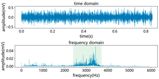
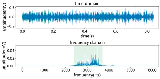
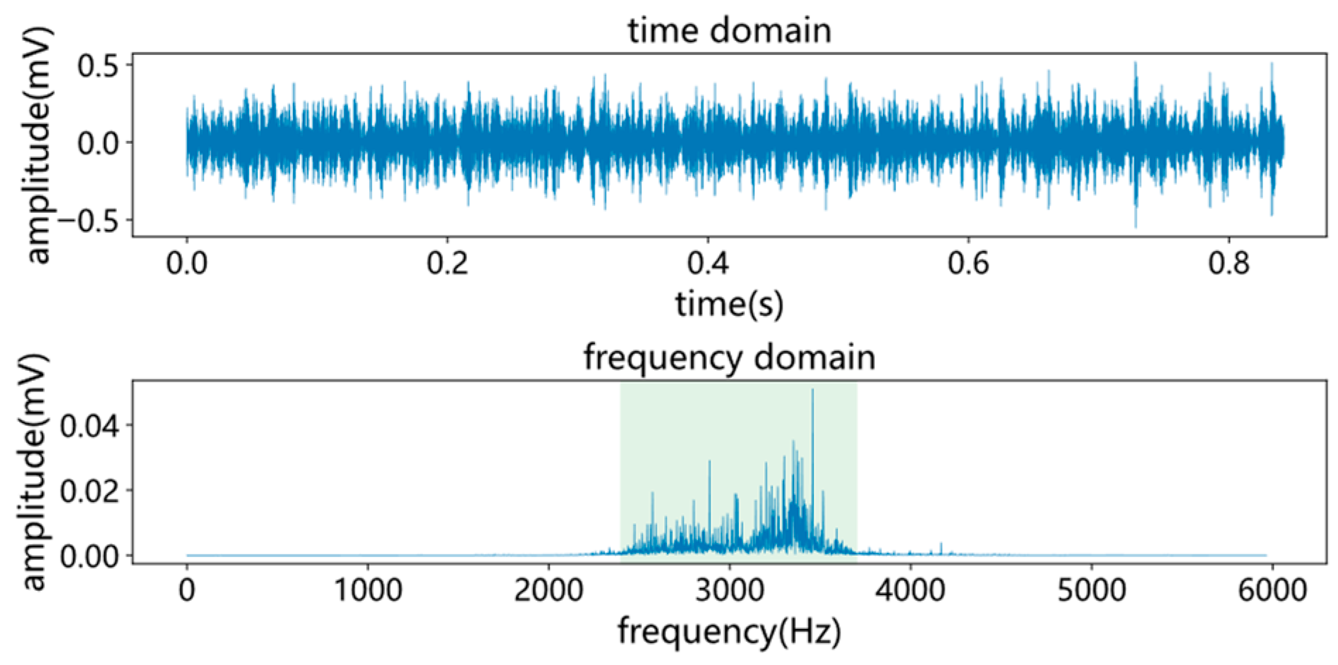
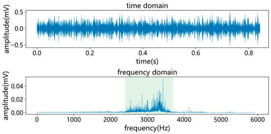
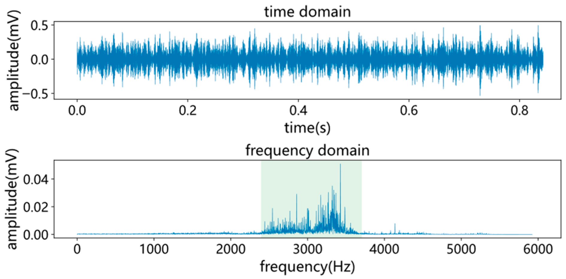
To validate the denoising performance, a vibration signal collected under the condition of 1600 r/min, 7 kN load, and rolling element pitting was selected as a case study. The time-domain and frequency-domain waveforms of the raw signal are presented in Figure 12.

Figure 12. Time and frequency domain diagram of fault signal before denoising. The green color indicates the critical frequency range.

The raw vibration signal and its frequency spectrum, depicted in Figure 12, exhibit significant background noise and irregular characteristics in the time domain. To address this, the BA-VMD algorithm was employed to decompose the signal. Based on signal complexity and literature reviews [14,34], the search bounds for the VMD parameters were established. Specifically, the number of $K$ was constrained to [2, 15] to prevent under-decomposition given the rich harmonics and strong noise of subway traction motors. The penalty factor ($\alpha$) was set to [300, 15,000] to balance narrow-band and wide-band characteristics. The hyperparameters for the Bat Algorithm were set as shown in Table 11.

Table 11. Parameter for BA-VMD.

Parameter	Value
Population size	20
Iterations	50
Variable dimensions	2
Modal component K	[2–15]
Penalty factor α	[300, 15,000]
Noise tolerance tau	0
Initial frequency estimate init	0
Convergence tolerance tol	1 × 10−6

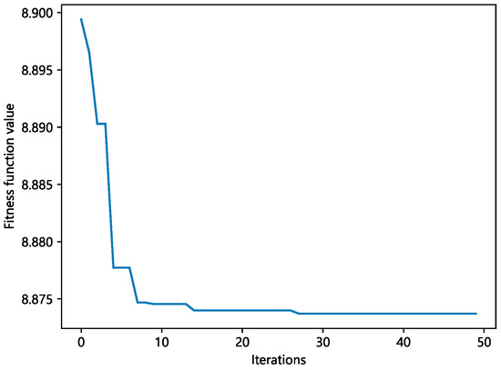
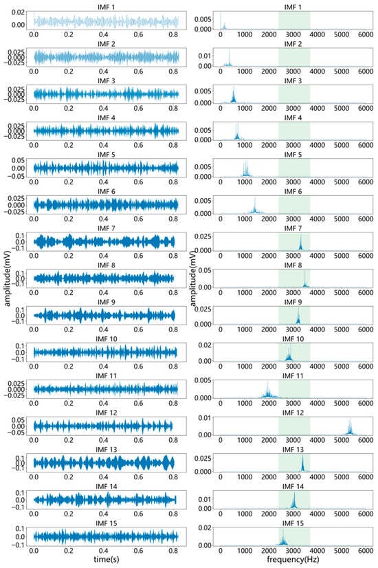
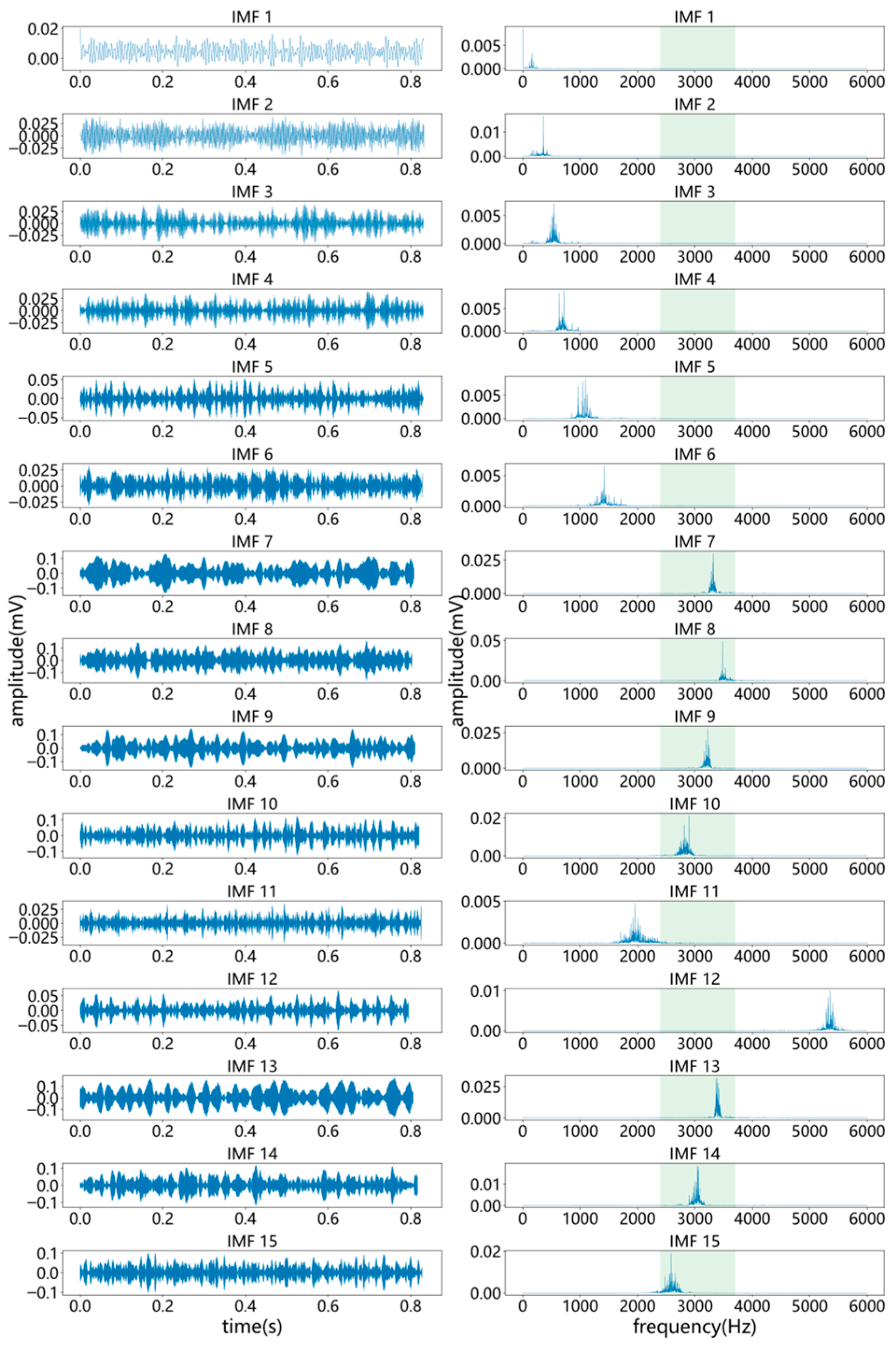
Figure 13 illustrates the convergence process of the Bat Algorithm. It is observed that the algorithm converges rapidly, stabilizing after approximately 7 iterations. The optimal parameter set was identified as K = 15 and α = 11,683. Using these parameters, the signal was decomposed into 15 Intrinsic Mode Functions (IMFs), as shown in Figure 14. The distinct time-frequency characteristics of these components, without modal aliasing, confirm the efficacy of the parameter optimization.

Figure 13. Convergence process of the BA-VMD algorithm fitness function during parameter optimization.

Figure 14. Time and frequency domain plots of BA-VMD modal components. The green color indicates the critical frequency range.

4.1.1. Noise Reduction and Component Selection

To reconstruct the denoised signal, the correlation between each IMF and the original signal was calculated. Table 12 lists the Pearson correlation coefficients for all 15 components. Based on the analysis of the fault characteristic frequency bands, a threshold of 0.27 was established to distinguish between signal-dominant and noise-dominant components. Consequently, the strongly correlated components—IMF7, IMF8, IMF9, IMF10, IMF13, IMF14, and IMF15—were selected for signal reconstruction.

Table 12. Correlation coefficient of modal components.

Modal Components	Correlation Coefficient
IMF1	0.0776
IMF2	0.1286
IMF3	0.1283
IMF4	0.1244
IMF5	0.1359
IMF6	0.0983
IMF7	0.4661
IMF8	0.4483
IMF9	0.4180
IMF10	0.3491
IMF11	0.1023
IMF12	0.0238
IMF13	0.5498
IMF14	0.3482
IMF15	0.2778

The time-domain and frequency-domain representations of the reconstructed signal are presented in Figure 15. Compared to the raw signal in Figure 12, the denoised waveform exhibits significantly clearer periodic impulses and reduced interference spectrum lines, indicating effective noise suppression.

Figure 15. Time and frequency domain plots of the fault signal after denoising. The green color indicates the critical frequency range.

4.1.2. Comparative Analysis

To objectively evaluate the performance of BA-VMD, a comparative study was conducted against Empirical Mode Decomposition (EMD) and standard VMD (with fixed parameters $K=5,\alpha =2000$).

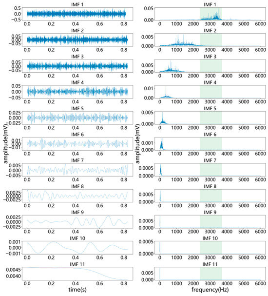
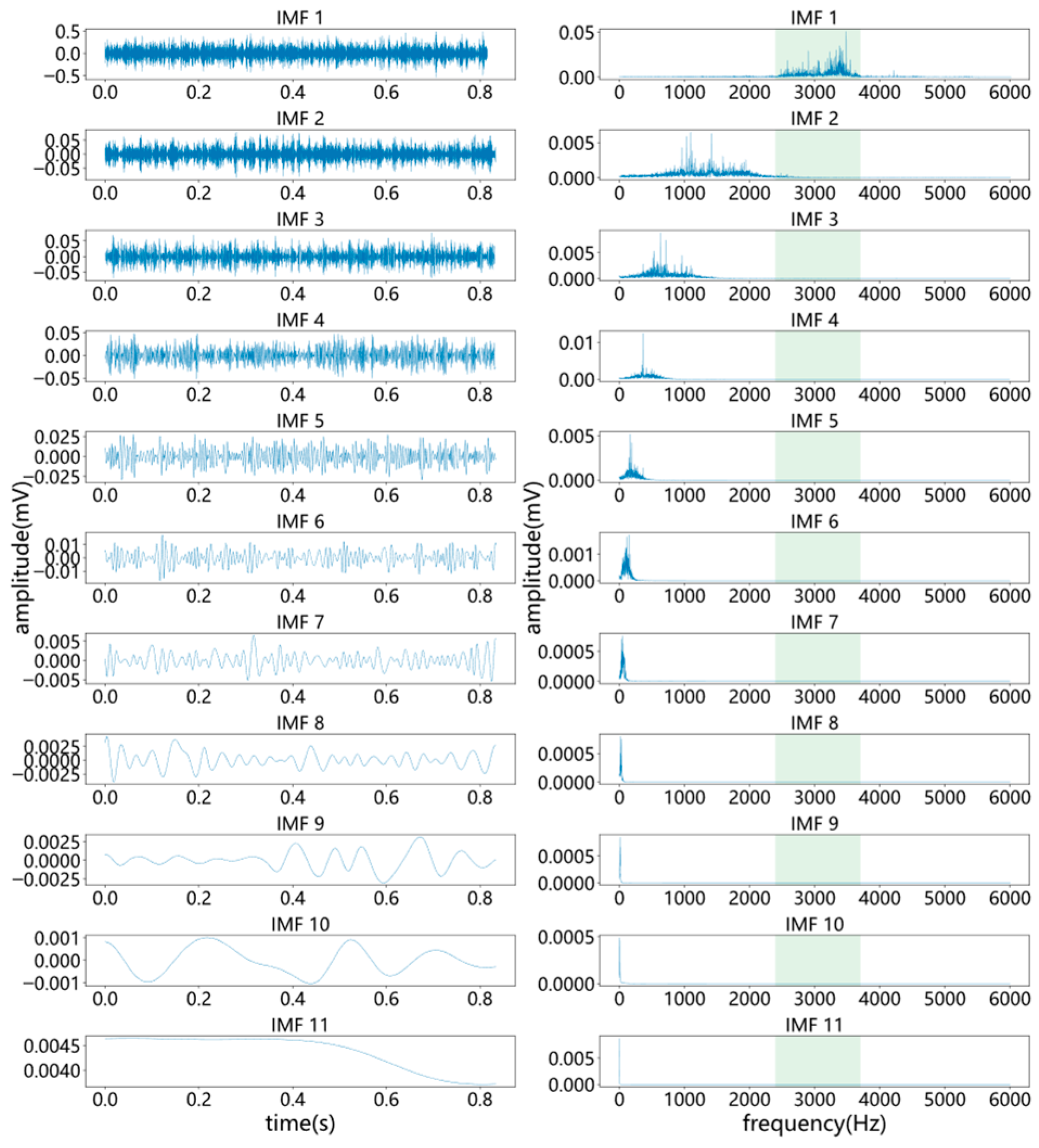
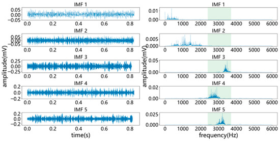
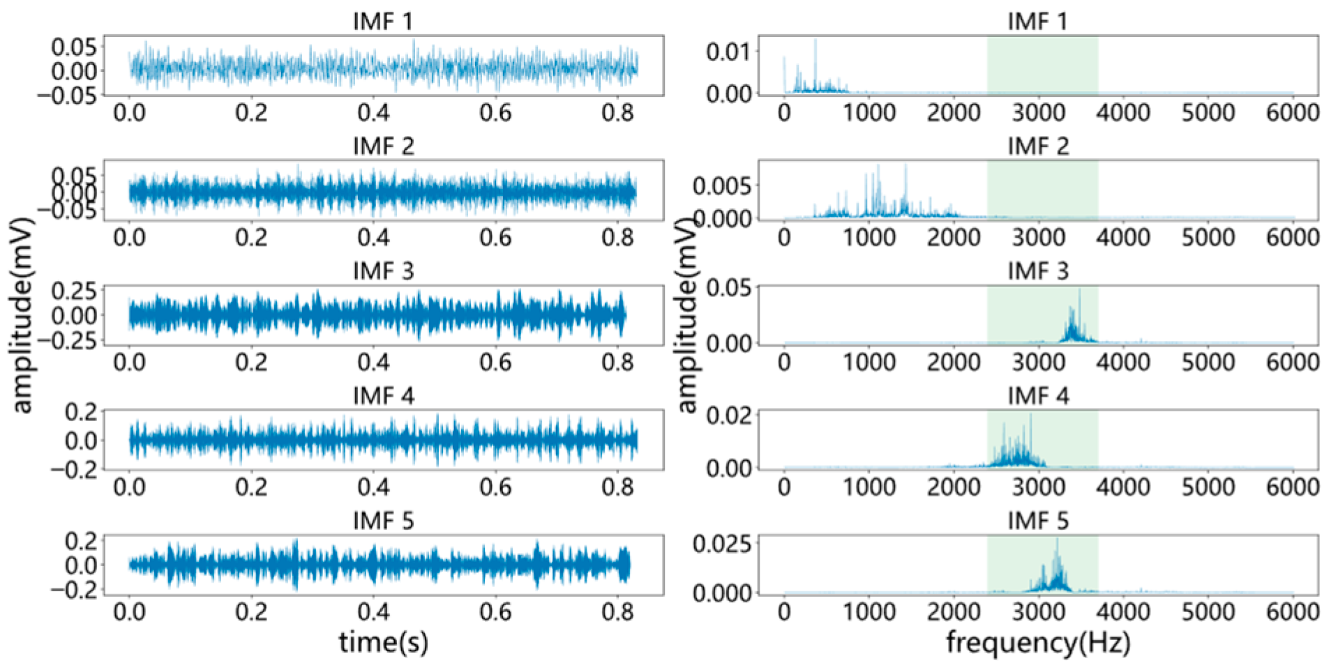
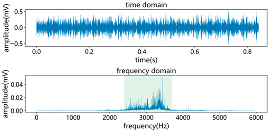
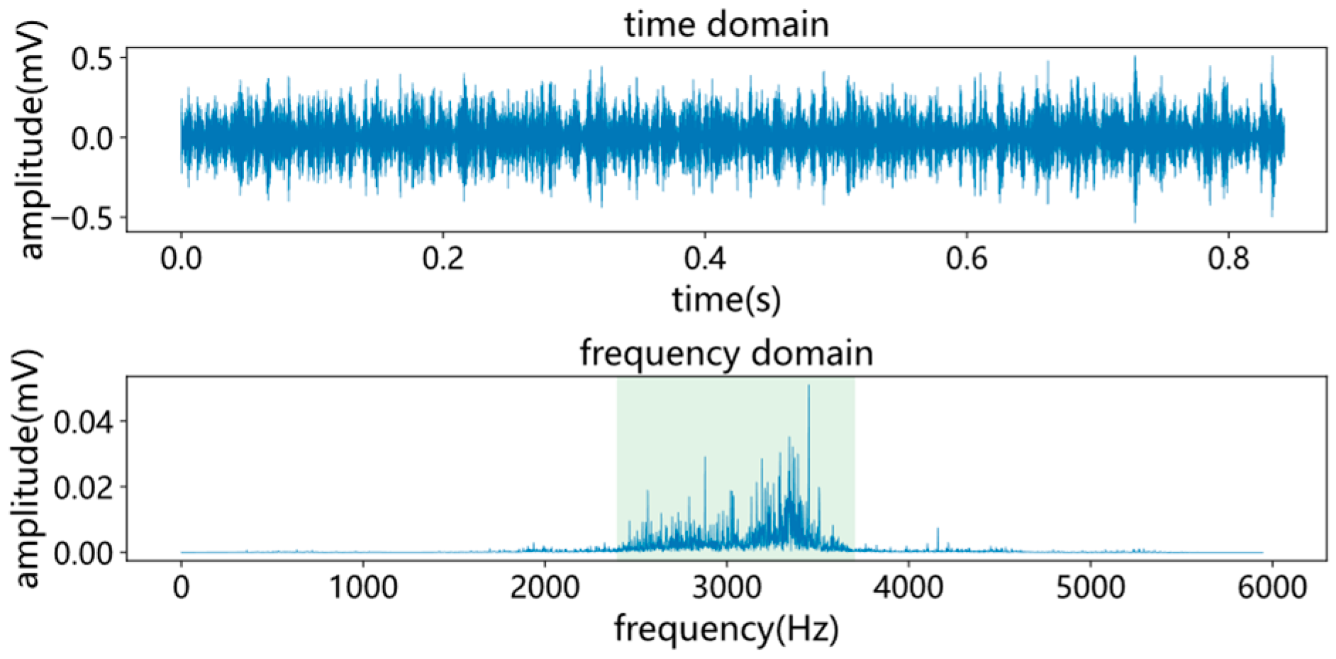
EMD Analysis: As shown in Figure 16, EMD suffers from severe mode aliasing, where the frequency-domain characteristics of the modal components are blurred. The reconstructed signal (Figure 17) retains significant noise interference, resulting in a low Signal-to-Noise Ratio.

Figure 16. Time and frequency domain plots of EMD modal components. The green color indicates the critical frequency range.

Figure 17. Time and frequency domain plots of the signal after EMD reconstruction. The green color indicates the critical frequency range.

Standard VMD Analysis: The standard VMD method (Figure 18) also fails to fully separate noise components due to suboptimal fixed parameters. The reconstructed signal (Figure 19) contains residual interference, yielding an SNR of only 5.64.

Figure 18. Time and frequency domain plots of VMD modal components. The green color indicates the critical frequency range.

Figure 19. Time and frequency domain plots of the signal after VMD reconstruction. The green color indicates the critical frequency range.

Quantitative Evaluation:

The denoising performance was quantitatively assessed using the Signal-to-Noise Ratio (SNR). The results, summarized in Table 13, demonstrate that the BA-VMD method achieves an SNR of 6.791. This represents a substantial improvement over EMD (5.196) and standard VMD (5.64). The results validate that the bat algorithm-optimized parameters are essential for achieving superior denoising performance on complex traction motor signals.

Table 13. Signal-to-noise ratio of different noise reduction methods.

Noise Reduction Method	Signal-to-Noise Ratio
EMD	5.196
VMD	5.64
BA-VMD	6.791

4.2. Experimental Analysis of Bearing Fault Diagnosis Based on Information Fusion of SA-CNN

4.2.1. Parameter Settings

The SA-CNN model was trained using the Adam optimization algorithm with a batch size of 50 and a learning rate of 0.001. Dropout regularization (rate = 0.3) was applied to the fully connected layer. The detailed network architecture is listed in Table 14.

Table 14. Structural parameters of SA-CNN network.

Network Layer	Input Size	Filter Size	Stride	Number of Filters	Filling	Output Size
Attention	128 × 128	-	-	-	-	128 × 128
Conv-1	128 × 128	3 × 3	1	16	1	128 × 128
Maxpool-1	128 × 128	2 × 2	2	-		64 × 64
Conv-2	64 × 64	3 × 3	1	32	1	64 × 64
Maxpool-2	64 × 64	2 × 2	2	-	-	32 × 32
Self-Attention	32 × 32	-	-	-	-	32 × 32
Conv-3	32 × 32	3 × 3	1	64	1	32 × 32
Maxpool-3	32 × 32	2 × 2	2	-	-	16 × 16
Conv-4	16 × 16	3 × 3	1	128	1	16 × 16
Maxpool-4	16 × 16	2 × 2	2	-	-	8 × 8
Fc, Dropout, LN, Softmax

4.2.2. Analysis of Bearing Fault Diagnosis Experimental Results

Single Operating Condition: For fault diagnosis under single operating conditions, the dataset for each condition was partitioned into training and testing sets at a ratio of 4:1. The fault diagnosis model was trained using the training set and subsequently evaluated on the testing set. The specific diagnostic protocol is detailed in Table 15.

Table 15. Bearing Failure Diagnosis Mode under Single Operating Condition.

Working Conditions	Training Set	Test Set
800 r/min, 5 kN	400	100
800 r/min, 7 kN	400	100
800 r/min, 9 kN	400	100
1600 r/min, 5 kN	400	100
1600 r/min, 7 kN	400	100
1600 r/min, 9 kN	400	100
2400 r/min, 5 kN	400	100
2400 r/min, 7 kN	400	100
2400 r/min, 9 kN	400	100

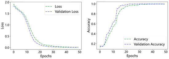
The SA-CNN model was trained for 50 epochs. Figure 20 illustrates the loss function and accuracy curves for the fusion signal under the condition of 1600 r/min and 7 kN. The model demonstrates stable convergence by the 20th epoch, indicating effective training performance.

Figure 20. Training loss and validation accuracy curves of the SA-CNN model under single operating conditions (1600 r/min, 7 kN).

The diagnostic results under single operating conditions are presented in Table 16. The fusion signal achieved an average accuracy of 99.06%, significantly outperforming the vibration signal (94.40%) and the acoustic emission signal (80.60%). This confirms that while vibration signals alone provide better diagnostic results than acoustic emission signals, the integration of multi-source signals further enhances diagnostic precision.

Table 16. Bearing fault diagnosis results under a single working condition.

Working Conditions	Acoustic Emission (%)	Vibration (%)	Fusion (%)
800 r/min, 5 kN	79.00	93.28	98.14
800 r/min, 7 kN	78.14	94.42	98.57
800 r/min, 9 kN	80.28	92.00	98.71
1600 r/min, 5 kN	80.00	94.00	99.00
1600 r/min, 7 kN	80.57	94.14	99.14
1600 r/min, 9 kN	80.42	95.00	100.00
2400 r/min, 5 kN	83.71	96.14	99.00
2400 r/min, 7 kN	82.00	95.14	99.28
2400 r/min, 9 kN	81.28	95.42	99.00

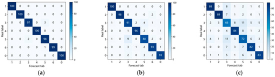
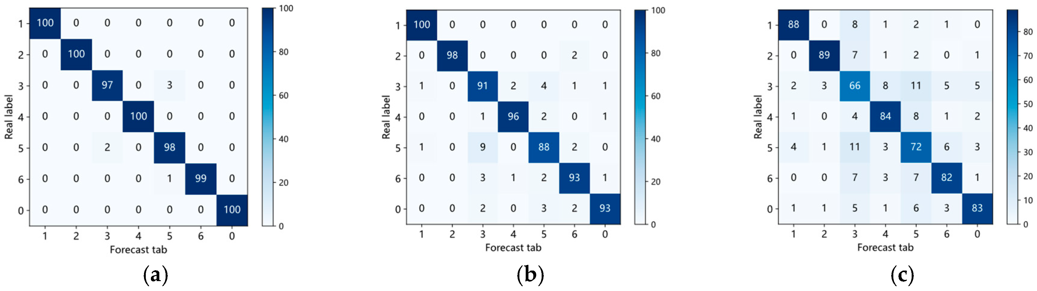
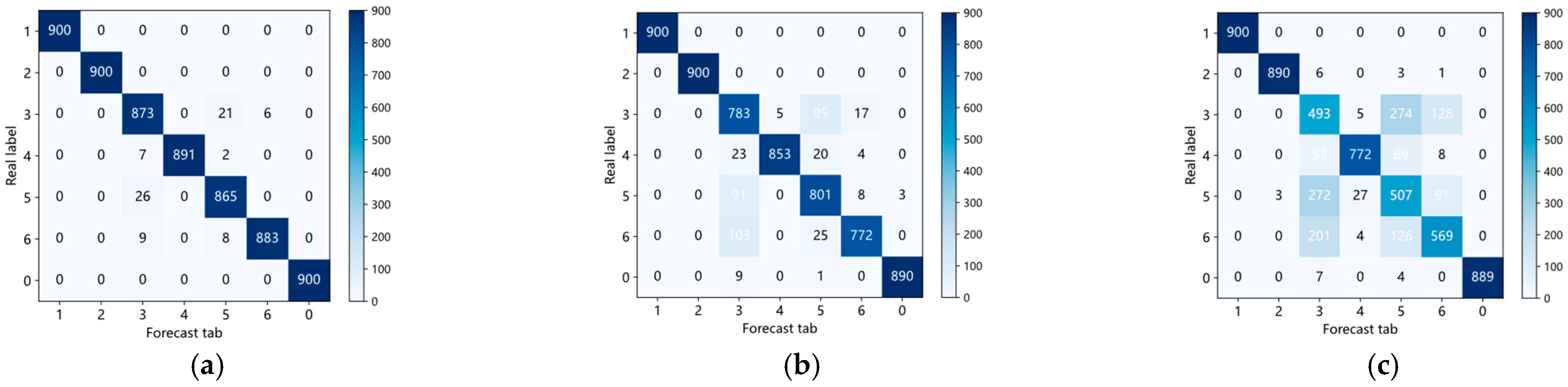
Figure 21 visualizes the confusion matrices for the 1600 r/min, 7 kN condition. Notably, the vibration signal exhibits some confusion between label “3” (Outer Ring Pitting) and label “5” (Inner Ring Crack). In contrast, the fusion signal achieves near-perfect classification, demonstrating that multi-signal integration effectively resolves ambiguities in fault identification.

Figure 21. Confusion matrix of fault diagnosis results under single operating conditions. (a) Fusion signal. (b) Vibration signal. (c) Acoustic emission signal.

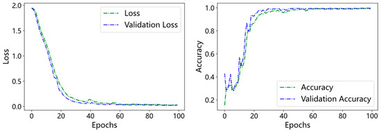
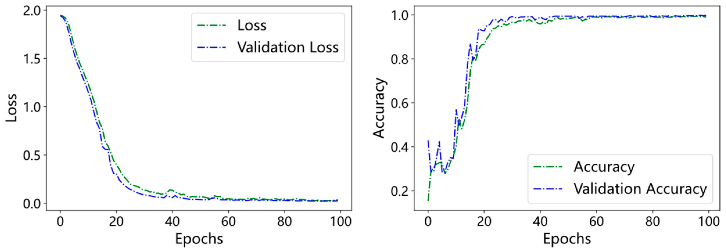
Variable Operating Conditions: To evaluate the model’s robustness under complex, variable working conditions, all samples from the nine operating conditions were aggregated and split into training and testing sets at a 4:1 ratio. The model was trained for 100 epochs. Figure 22 depicts the loss and accuracy curves for the fusion signal under these variable conditions. The model exhibits stable convergence by the 50th epoch.

Figure 22. Training loss and validation accuracy curves of the SA-CNN model under variable working conditions.

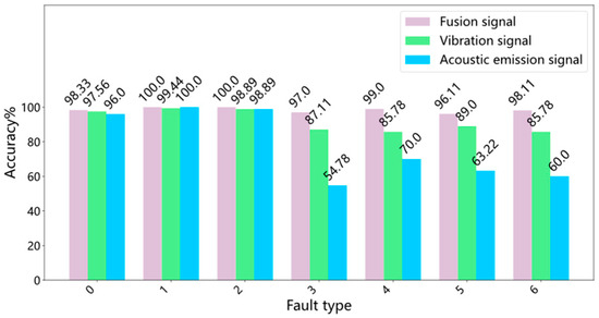
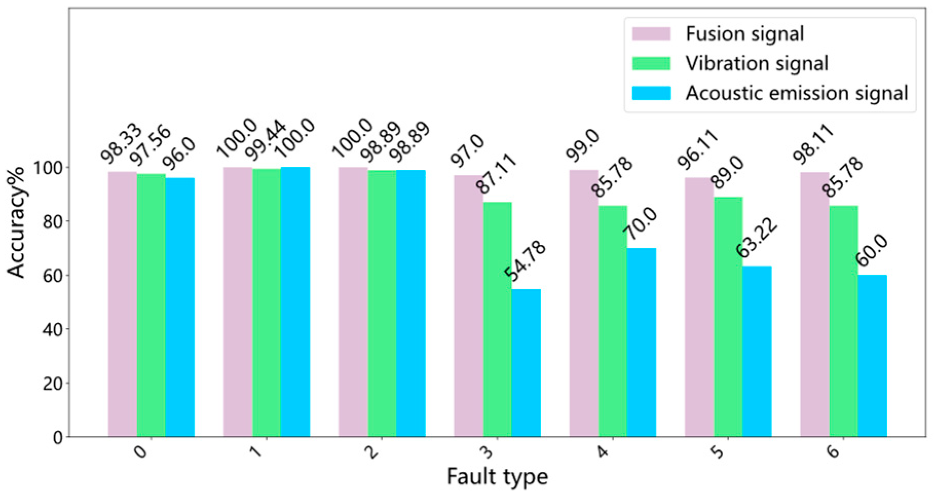
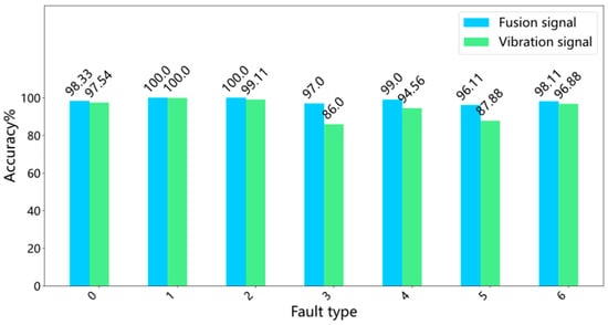
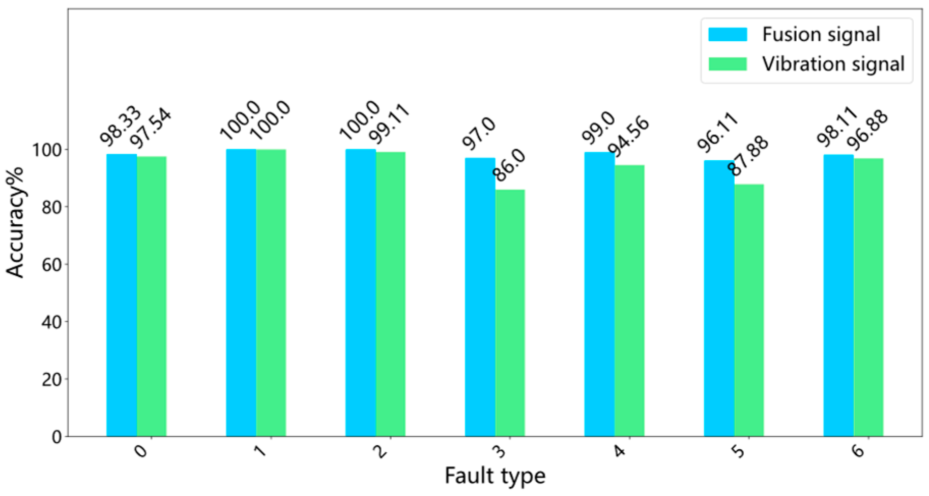
The diagnostic results are summarized in Figure 23 and Figure 24. Although the accuracy is slightly lower than in single-condition scenarios due to increased data complexity, the fusion signal maintains a high average accuracy of 98.60%, significantly surpassing the vibration (93.63%) and acoustic emission (79.60%) signals. These results confirm the stability and reliability of the proposed method under variable operating conditions.

Figure 23. Comparison of diagnostic accuracy among fusion signals, vibration signals, and acoustic emission signals under variable working conditions.

Figure 24. Confusion matrix of fault diagnosis results under variable operating conditions. (a) Fusion signal. (b) Vibration signal. (c) Acoustic emission signal.

4.2.3. Comparative Experimental Analysis

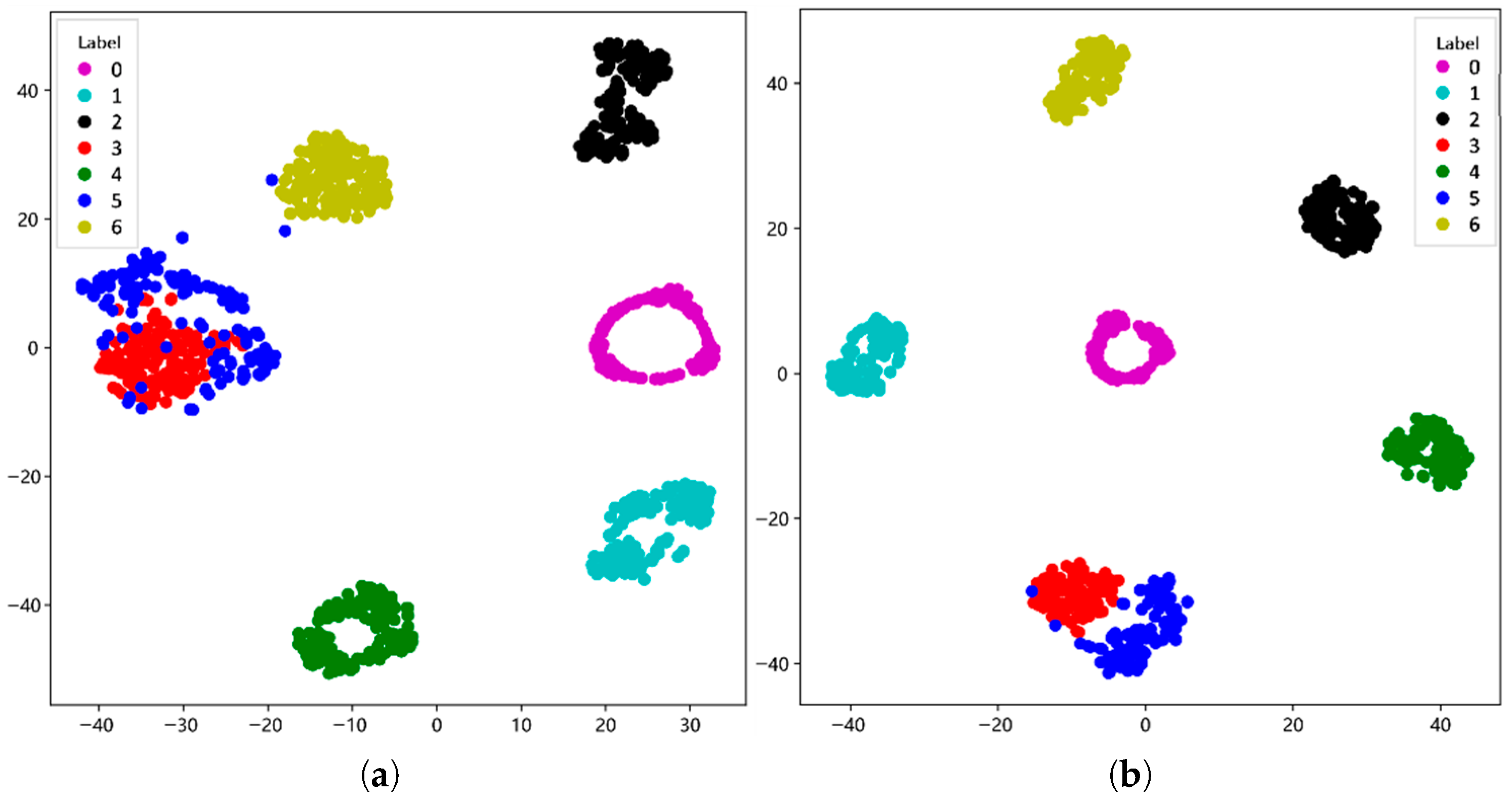
Comparative Experiment 1: To validate the contribution of the Self-Attention (SA) module to feature extraction, the t-SNE algorithm was employed to visualize the feature distributions before and after the integration of the SA module. Figure 25a,b depict the feature clustering results prior to and subsequent to the application of the self-attention mechanism, respectively.

Figure 25. Comparison of feature clustering performance between the CNN model and the SA-CNN model using t-SNE visualization. (a) Before SA. (b) After SA.

An analysis of the feature distributions reveals that after the second convolution-pooling layer, while certain fault categories are distinguishable, significant inter-class confusion persists. Specifically, the boundaries between fault types “3” (Outer Ring Pitting) and “5” (Inner Ring Crack) are ambiguous, indicating that the model struggles to differentiate between these similar fault patterns at this stage. In contrast, following the Self-Attention module, the features corresponding to the seven fault types form distinct, compact clusters with clear decision boundaries. This demonstrates that the self-attention mechanism effectively enhances the model’s ability to extract discriminative features and suppress irrelevant information, thereby significantly improving classification performance.

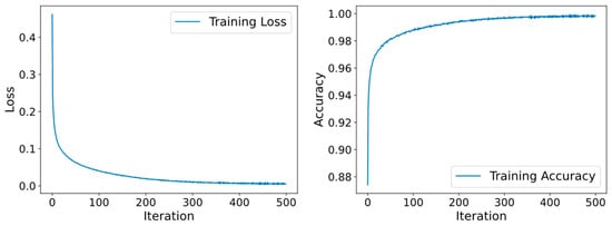
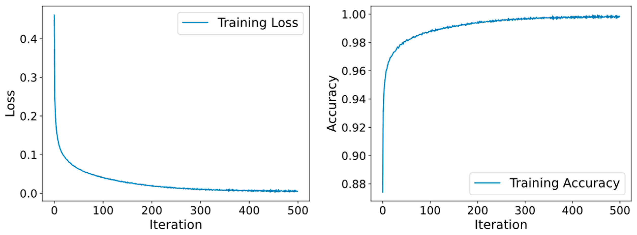
Comparative experiment 2: The proposed SA-CNN was compared with Multilayer Perceptron (MLP) and Support Vector Machine (SVM) models. The MLP was configured with 16 hidden units, and other hyperparameters were kept consistent with the SA-CNN to ensure a fair comparison. The MLP was trained for 500 epochs.

Figure 26 shows the loss and accuracy curves for the MLP. The MLP loss function stabilizes around the 200th iteration, indicating that the SA-CNN model converges significantly faster. The diagnostic accuracies of the different methods are compared in Table 17. The SA-CNN achieves the highest accuracy of 98.60%, outperforming both MLP (93.57%) and SVM (90.90%).

Figure 26. Curves of loss function and accuracy variation of fused signals for MLP fused signals.

Table 17. Comparison of diagnostic accuracies among different methods (Mean ± Std).

Model	Accuracy (%)
MLP	93.57 ± 0.98
SVM	90.90 ± 1.25
SA-CNN	98.60 ± 0.35

To verify the statistical significance of these improvements, a paired t-test was conducted (Table 18). The p-values for comparisons between SA-CNN and the baseline methods are well below 0.05, confirming that the performance improvement is statistically significant.

Table 18. Paired t-test results between SA-CNN and baseline methods.

Comparison	p-Value	Significant? ($\mathit{\alpha }=0.05$)
SA-CNN vs. SVM	0.00012	Yes
SA-CNN vs. MLP	0.00345	Yes

Comparative experiment 3: To validate the efficacy of the proposed attention-based fusion strategy, it was compared with a parallel convolutional CNN fusion method. The results are presented in Table 19 and Figure 27.

Table 19. Diagnostic accuracy of different fusion methods.

Model	Accuracy (%)
Parallel convolutional CNN	94.28
SA-CNN	98.60

Figure 27. Comparison of diagnostic accuracy between parallel convolutional CNN and SA-CNN using fusion signals and vibration signals.

The SA-CNN method achieved an accuracy of 98.60%, compared to 94.28% for the parallel convolutional CNN. This indicates that the attention mechanism effectively captures the correlation between different information sources and assigns appropriate weights to fault features, thereby improving diagnostic accuracy compared to simple feature concatenation.

5. Conclusions

This study presents a novel bearing fault diagnosis framework tailored for subway traction motors, integrating BA-VMD denoising and SA-CNN information fusion. Through systematic experiments, the proposed method demonstrates superior performance in handling noisy signals and complex fault patterns under variable operating conditions. The specific conclusions are as follows:

First, the proposed BA-VMD method significantly enhances signal quality.Compared to traditional EMD and standard VMD, the Bat Algorithm effectively optimizes the VMD parameters ($K=15, \alpha =11,683$), resolving the issues of modal aliasing and endpoint effects. As demonstrated in the denoising experiments, this approach achieves a Signal-to-Noise Ratio (SNR) of 6.791, which represents a substantial improvement over EMD (5.196) and standard VMD (5.64). The distinct time-frequency characteristics of the decomposed components confirm the efficacy of this denoising strategy in extracting weak fault features from heavy background noise.

Second, the SA-CNN model demonstrates exceptional robustness in multi-source information fusion under variable operating conditions. Specifically designed to address the challenges of fluctuating speeds and loads, the model achieves a remarkable average diagnostic accuracy of 98.60% when tested across nine distinct operating conditions. This highlights the model’s strong generalization capability in complex environments. Furthermore, the Self-Attention mechanism effectively resolves the classification ambiguity between similar fault types (specifically Label 3 and Label 5) by dynamically weighting vibration and acoustic emission signals. Comparative experiments validate that the proposed method significantly outperforms traditional models such as MLP (93.57%) and SVM (90.90%), as well as the Parallel Convolutional CNN method (94.28%).

Third, regarding practical application, the proposed method is computationally efficient for real-time deployment. While the model training is complex and performed offline, the inference phase involves only forward propagation. Given the lightweight architecture of the SA-CNN, the computational cost during inference is low, demonstrating its suitability for real-time fault detection on modern industrial embedded systems.

Despite these promising results, several avenues for future research remain. Future work will focus on further optimizing the parameter configurations of the BA-VMD and SA-CNN models to enhance diagnostic performance. Additionally, the scope of fault types will be expanded to improve the model’s generalization ability. Finally, we will explore the fusion of data from other sensor types, such as temperature and current, to achieve a more comprehensive assessment of bearing health and further improve diagnostic reliability.

References

- Meng, Z.; Wang, X.; Liu, J.; Fan, F. An Adaptive Spectrum Segmentation-Based Optimized VMD Method and Its Application in Rolling Bearing Fault Diagnosis. Meas. Sci. Technol. 2022, 33, 125107. [Google Scholar] [CrossRef] [Scilit]
- Meng, Z.; Liu, J.; Liu, J.; Li, J.; Cao, L.; Fan, F.; Yu, S. An Improved Variational Mode Decomposition Method Based on Spectrum Reconstruction and Segmentation and Its Application in Rolling Bearing Fault Diagnosis. Digit. Signal Process. 2023, 141, 104161. [Google Scholar] [CrossRef] [Scilit]
- Smith, W.A.; Randall, R.B. Rolling Element Bearing Diagnostics Using the Case Western Reserve University Data: A Benchmark Study. Mech. Syst. Signal Process. 2015, 64–65, 100–131. [Google Scholar] [CrossRef] [Scilit]
- Wei, S.; Wang, D.; Wang, H.; Peng, Z. Time-Varying Envelope Filtering for Exhibiting Space Bearing Cage Fault Features. IEEE Trans. Instrum. Meas. 2021, 70, 3504313. [Google Scholar] [CrossRef] [Scilit]
- Zuo, J.; Lin, J.; Miao, Y. Period Enhanced Feature Mode Decomposition and Its Application for Bearing Weak Fault Feature Extraction. Meas. Sci. Technol. 2024, 35, 116127. [Google Scholar] [CrossRef] [Scilit]
- Donoho, D.L.; Johnstone, I.M. Adapting to Unknown Smoothness via Wavelet Shrinkage. J. Am. Stat. Assoc. 1995, 90, 1200–1224. [Google Scholar] [CrossRef]
- Huang, N.E.; Shen, Z.; Long, S.R.; Wu, M.C.; Shih, H.H.; Zheng, Q.; Yen, N.-C.; Tung, C.C.; Liu, H.H. The Empirical Mode Decomposition and the Hilbert Spectrum for Nonlinear and Non-Stationary Time Series Analysis. Proc. A 1998, 454, 903–995. [Google Scholar] [CrossRef] [Scilit]
- Ma, Z.; Zhang, Y. A Study on Rolling Bearing Fault Diagnosis Using RIME-VMD. Sci. Rep. 2025, 15, 4712. [Google Scholar] [CrossRef] [Scilit]
- Zhou, J.; Xiao, M.; Niu, Y.; Ji, G. Rolling Bearing Fault Diagnosis Based on WGWOA-VMD-SVM. Sensors 2022, 22, 6281. [Google Scholar] [CrossRef] [Scilit] [PubMed]
- Liu, B.; Hao, X. Research on Anti-Frequency Sweeping Jamming Method for Frequency Modulation Continuous Wave Radio Fuze Based on Wavelet Packet Transform Features. Appl. Sci. 2022, 12, 8713. [Google Scholar] [CrossRef] [Scilit]
- Chao, Z.; Han, T. A Novel Convolutional Neural Network with Multiscale Cascade Midpoint Residual for Fault Diagnosis of Rolling Bearings. Neurocomputing 2022, 506, 213–227. [Google Scholar] [CrossRef] [Scilit]
- Liu, Z.; Sun, W.; Chang, S.; Zhang, K.; Ba, Y.; Jiang, R. Corn Harvester Bearing Fault Diagnosis Based on ABC-VMD and Optimized EfficientNet. Entropy 2023, 25, 1273. [Google Scholar] [CrossRef] [Scilit] [PubMed]
- You, J.; Zhi, Z.; Gao, Y. Research on Fault Diagnosis of Motor Bearings Based on SBOA-VMD-TCN. IEEE Access 2025, 13, 174815–174830. [Google Scholar] [CrossRef] [Scilit]
- Dragomiretskiy, K.; Zosso, D. Variational Mode Decomposition. IEEE Trans. Signal Process. 2014, 62, 531–544. [Google Scholar] [CrossRef] [Scilit]
- Lu, Q.; Shen, X.; Wang, X.; Li, M.; Li, J.; Zhang, M. Fault Diagnosis of Rolling Bearing Based on Improved VMD and KNN. Math. Probl. Eng. 2021, 2021, 2530315. [Google Scholar] [CrossRef] [Scilit]
- Xiang, N.; Zhang, T.; Liu, Y. State of Health Prediction for Lithium-Ion Batteries Using Extended Long Short-Term Memory Network and Frequency Enhanced Channel Attention Mechanism with Variational Mode Decomposition. Measurement 2025, 249, 117084. [Google Scholar] [CrossRef] [Scilit]
- Liu, J.; Zhang, Y.; Wen, K.; Ding, Y. Analysis of Different Neural Network Models Based on Variational Mode Decomposition and Dung Beetle Optimizer Algorithm for the Prediction of Air-Conditioning Energy Consumption in Multifunctional Complex Large Public Buildings. Energy Build. 2025, 334, 115518. [Google Scholar] [CrossRef] [Scilit]
- Wang, D.; Tong, Y.; Yang, D.; Wang, P.; Lu, J. Optimized Variational Mode Decomposition Denoising Method Based on Weighted Mean of Vectors Algorithm. Pet. Sci. Technol. 2025, 43, 949–966. [Google Scholar] [CrossRef] [Scilit]
- Yang, M.; Zhou, Q.; Huang, H.; Liu, J.; Pan, H.; Cheng, Y.; Kang, Z.; Hu, Z.; Hu, Y. A Fault Prediction Method for CMOR Bearings Based on Parameter-Optimized Variational Mode Decomposition and Autocorrelation Function. Fusion Eng. Des. 2025, 212, 114863. [Google Scholar] [CrossRef] [Scilit]
- Fahim, S.R.; Sarker, Y.; Sarker, S.K.; Sheikh, M.R.I.; Das, S.K. Self Attention Convolutional Neural Network with Time Series Imaging Based Feature Extraction for Transmission Line Fault Detection and Classification. Electr. Power Syst. Res. 2020, 187, 106437. [Google Scholar] [CrossRef] [Scilit]
- Tong, J.; Liu, C.; Zheng, J.; Pan, H. Multi-Sensor Information Fusion and Coordinate Attention-Based Fault Diagnosis Method and Its Interpretability Research. Eng. Appl. Artif. Intell. 2023, 124, 106614. [Google Scholar] [CrossRef] [Scilit]
- Yang, X.-S. A New Metaheuristic Bat-Inspired Algorithm. In Nature Inspired Cooperative Strategies for Optimization (NICSO 2010); González, J.R., Pelta, D.A., Cruz, C., Terrazas, G., Krasnogor, N., Eds.; Springer: Berlin/Heidelberg, Germany, 2010; pp. 65–74. ISBN 978-3-642-12538-6. [Google Scholar]
- Wang, T.; Xie, M. IBBA: An Improved Binary Bat Algorithm for Solving Low and High-Dimensional Feature Selection Problems. Int. J. Mach. Learn. Cybern. 2025, 16, 5605–5635. [Google Scholar] [CrossRef] [Scilit]
- Bai, Y.; Sun, D.; Liu, L.; Shen, Y.; Yao, H. Energy-Saving Optimization of Air-Conditioning Water System Based on Machine Learning and Improved Bat Algorithm. Energy Build. 2025, 332, 115333. [Google Scholar] [CrossRef] [Scilit]
- Laamari, M.A.; Kamel, N. A New Multi-Objective Binary Bat Algorithm for Feature Selection in Intrusion Detection Systems. Concurr. Comput. Pract. Exp. 2025, 37, e70000. [Google Scholar] [CrossRef] [Scilit]
- Bahdanau, D.; Cho, K.; Bengio, Y. Neural Machine Translation by Jointly Learning to Align and Translate. arXiv 2014, arXiv:1409.0473. [Google Scholar]
- Zhang, W.; Yang, J.; Bo, X.; Yang, Z. A Dual Attention Mechanism Network with Self-Attention and Frequency Channel Attention for Intelligent Diagnosis of Multiple Rolling Bearing Fault Types. Meas. Sci. Technol. 2024, 35, 036112. [Google Scholar] [CrossRef] [Scilit]
- Liu, Y.; Zheng, W.; Du, Y.; Wang, Y.; Jin, J.; Yu, M. Bearing Fault Diagnosis Based on Cross Image Multi-Attention Mechanism. Sci. Rep. 2025, 15, 21100. [Google Scholar] [CrossRef] [Scilit]
- Vaswani, A.; Shazeer, N.; Parmar, N.; Uszkoreit, J.; Jones, L.; Gomez, A.N.; Kaiser, L.; Polosukhin, I. Attention Is All You Need. In Advances in Neural Information Processing Systems 30 (NIPS 2017); NeurIPS: Long Beach, CA, USA, 2017; pp. 5998–6008. [Google Scholar]
- Wu, Q.; Lin, H. Short-Term Wind Speed Forecasting Based on Hybrid Variational Mode Decomposition and Least Squares Support Vector Machine Optimized by Bat Algorithm Model. Sustainability 2019, 11, 652. [Google Scholar] [CrossRef] [Scilit]
- Yan, X.; Shi, Z.; Sun, Z.; Zhang, C.-A. Multisensor Fusion on Hypergraph for Fault Diagnosis. IEEE Trans. Ind. Inform. 2024, 20, 10008–10018. [Google Scholar] [CrossRef] [Scilit]
- GB/T 283-2021; Rolling Bearings—Cylindrical Roller Bearings and Inner Rings—Boundary Dimensions and Tolerances. Standards Press of China: Beijing, China, 2021.
- Randall, R.B.; Antoni, J. Rolling Element Bearing Diagnostics—A Tutorial. Mech. Syst. Signal Process. 2011, 25, 485–520. [Google Scholar] [CrossRef] [Scilit]
- Zhang, X.; Miao, Q.; Zhang, H.; Wang, L. A Parameter-Adaptive VMD Method Based on Grasshopper Optimization Algorithm to Analyze Vibration Signals from Rotating Machinery. Mech. Syst. Signal Process. 2018, 108, 58–72. [Google Scholar] [CrossRef] [Scilit]
Disclaimer/Publisher’s Note: The statements, opinions and data contained in all publications are solely those of the individual author(s) and contributor(s) and not of MDPI and/or the editor(s). MDPI and/or the editor(s) disclaim responsibility for any injury to people or property resulting from any ideas, methods, instructions or products referred to in the content. |
© 2026 by the authors. Licensee MDPI, Basel, Switzerland. This article is an open access article distributed under the terms and conditions of the Creative Commons Attribution (CC BY) license.