A Method for Load Distribution Used in Multi-Server Environments

Abstract

A novel scheme is proposed to provide power-saving and prevent server overload in multi-server network environments. It is achieved by partitioning the service capacity of each load server into a sum of its ratio and combining with a switching strategy among servers. Conditions for the choice of the ratio are obtained to guarantee the avoidance of server overload. Two switching strategies among multiple servers are also proposed for even distribution and energy saving in different applications. Simulation results are presented to demonstrate the success of the proposed design.

1. Introduction

As the internet becomes increasingly widespread, numerous applications have been developed, such as Web-based services, cloud computing, three-dimensional communication networks, and the Internet of Things (IoT) (e.g., [1,2,3,4,5,6,7]). In these schemes, distributing server load across multiple servers/nodes is considered a crucial issue for optimizing resource utilization. It is known that every system server has limitations in computation power when answering client requests. Once incoming requests exceeds the server’s allowed connection numbers, it would become overloaded and malfunction. To avoid such a problem, the online administrators typically add more servers to share the connection requests and meet client demand. Unfortunately, adding extra servers may not be able to solve the overload problem. As the mechanism for sharing the requests is not well taken care of, a large amount of connection requests might pour into some servers and cause them to break down. Hence, it is important to balance the connections among the servers of the system. The mechanism of distributing clients’ requests into a group of systems’ servers is known as “load distribution” or “server load balancing” [8,9,10,11,12,13,14].

Among the existing studies, the technologies of load balancing can be categorized into static and dynamic types [6,15]. The former allocates requests based on the known system information, and the latter distributes tasks based on the instant server status. Three static algorithms, including min–min, max–min and round robin, are known popular schemes for load balancing due to their simple working mechanism (e.g., [5,15,16,17,18]). The min–min algorithm proceeds by assigning the task to the resource that produces the minimum completion time. It first constructs the set U of the task–server pairs by finding the minimum execution time for each task across all available servers. Then it selects the task–server pair from U that yields the minimum completion time. The same procedure is repeated until all the tasks are scheduled (e.g., [15,16]). The max–min algorithm is similar to that of min–min algorithm but uses a different strategy for selecting the machine in the second step of the procedure.

Instead of choosing the minimum completion time, the max–min algorithm selects the task from the set U that has the maximum completion time to be performed by the corresponding server (e.g., [15,16]). The classic and widely used round robin algorithm is a procedure that distributes incoming requests to servers in a sequential and cyclical manner. It is a simple and easy-to-implement approach in which each server receives a fair share of requests in a rotational order. However, such a method does not take individual server loads or conditions into account, which might lead to some servers being overloaded if the requesting loads are not evenly distributed (e.g, [5,7]).

To improve service performance, several hybrid methods have been proposed that consider differing client usage patterns, such as sorting service providers based on dynamic time quantum [17] or classifying requests into different server groups before applying the round-robin algorithm based on size-interval task assignments [18]. Compared to the static round robin algorithm, the dynamic least connections method distributes requests based on the real-time connection count of servers. If the servers have identical specifications, the least connections scheme can achieve better average response time performance than the round robin method [5]. Another consideration is to prioritize servers based on a weighting factor derived from server specifications and/or instant server status (e.g., [7,19,20,21]). Incoming requests are subsequently assigned to the server with the highest priority. To prevent overload, current server capacity and task load are considered (e.g., [7,19,20]). The major difference among these proposals lies in the usage of a queued architecture on the server, which allows tasks to be shifted from heavily loaded servers to less loaded ones [19,20]. Another scheme prevents later requests from being allocated to overloaded servers [7]. In these designs, an overloaded server is defined as one whose instantaneous load exceeds a threshold value. Hence, if the threshold is not set appropriately, an overload problem may occur if the assigned client load exceeds the server’s remaining capacity.

Although request assignment based on load has been considered in existing algorithms such as the min–min and max–min methods (e.g., [15,16]), a lack of assessment regarding remaining server capacity is a major problem in these overload avoidance proposals. Several optimal algorithms have been recently proposed to tackle this issue due to increasing computational power (e.g., [22,23,24]). However, those studies pay more attention to optimizing service performance in complex environments. In addition to system performance, energy efficiency is a crucial factor in multi-server/node environments, such as data centers (e.g., [25,26]). Among existing studies, this issue is commonly formulated as an optimization problem (e.g., [25,27,28,29]), with two different core speed models proposed in [25]. Compared to [25], the work in [27] focuses on the interaction between load balancing and energy efficiency in software-defined networks, employing the Krill Herd (KH) meta-heuristic algorithm to construct a dynamic optimization scheme. However, it was reported in [28,29] that load balancing and energy efficiency might not be independent, as the algorithms for energy efficiency resulted in both balanced and imbalanced loads. In addition, the issue of auto-scaling has recently attracted significant attention in existing power reduction schemes [26,27,30].

In contrast to existing schemes, this study develops a simpler approach to solving the server overload problem based on its capacity. The proposed method combines two designs: partitioning the service capacity of each server and implementing a switching strategy for sharing and/or directing client request loads. While a preliminary concept was presented in [31,32] to justify the possibility of avoiding overload, this paper extends those previous results to derive conditions that guarantee the prevention of overload. Furthermore, we discuss potential switching strategies for power saving and auto-scaling of servers.

The organization of this paper is as follows. Section 2 provides a brief review of related works. Section 3 presents the proposed schemes for load distribution in a multi-server environment. Simulation results are given in Section 4 to demonstrate the effectiveness of the proposed design, followed by a discussion of the achievements in Section 5. Finally, Section 6 concludes the paper.

2. Related Works

In this section, we will first briefly review the literature related to the study of the paper. Details are given as follows.

It is known that the design of the so-called “load distribution” or “load balancing” technology plays a crucial role in avoiding server overloads in multi-server environments. Among those existing studies, several issues have been considered to enhance the performance of load distribution schemes. One major factor is “energy efficiency”, which is critical for the operation of multiple server/node environments, such as data centers (e.g., [26]). Consequently, this issue is generally treated as an optimization problem (e.g., [27,33,34,35,36]). Based on the formulation of an optimization problem, different models and designs have been proposed to construct schemes for load distribution. For instance, the interaction between load balancing and energy efficiency in software-defined networks was discussed and the Krill Herd (KH) meta-heuristic algorithm was employed to construct a dynamic optimization scheme [27]. A fully distributed computation offloading (FDCO) algorithm was constructed to solve the problem of distributed computation offloading decision-making among multiple mobile devices in a cloudlet-based mobile cloud computing system [33]. Additionally, a two-timescale online optimization approach was proposed to study the structure of human digital twins [34].

The challenges of load balancing and energy efficiency in a hybrid IP/Software-Defined Networking (SDN) structure were addressed in [35]. A so-called “Hybrid Spreading Load Algorithm (HSLA)” was proposed to tackle the defined mixed integer linear programming (MILP) formulation aimed at minimizing both maximum link utilization and the network power consumption. Additionally, an integration method was proposed to solve the multi-objective load balancing problem in a cloud environment [36]. This was achieved by combining Ant Colony Optimization (ACO) and Water Wave Optimization (WWO). Compared with several conventional optimization schemes, the study states that the proposed approach can enhance task scheduling efficiency while decreasing operational expenses and lowering energy usage.

Another issue is the “scalability” of the structure for serving machines to answer the incoming requests in a multi-server environment. Such a concern has recently become a crucial concept in several power reduction schemes [26,27,30,37,38]. The main focus of these load distribution mechanisms is the large power consumption difference between an active server and one in sleep mode. To handle the so-called “under-provisioning” and “over-provisioning” problems in cloud computing environments, a dynamically scalable architecture of virtual clusters was proposed in [37]. This proposed scheme consists of three key components: a front-end load balancer, a cluster monitoring system, and an auto-provisioning/auto-scaling algorithm. In this design, the front-end load balancer routes and balances all user requests across cloud services installed in the virtual cluster. The virtual cluster monitoring system collects information on the physical resource usage of all virtual machines. Subsequently, the auto-provisioning mechanism dynamically provisions virtual machines based on active session numbers or resource consumption. In addition, an auto-scaling technique was employed to guide the operation of the proposed architecture by monitoring the current bandwidth and active sessions of all virtual machines. New virtual machines are added to the front-end load balancer when the network bandwidth and active session of all virtual machines reach specified upper threshold values. Furthermore, a Markovian framework is proposed in [38] for load balancing and allowing the network service capacity to be scalable in response to the current load on the same timescale as job dynamics. This is achieved by combining classical algorithms such as Power-of-d with auto-scaling mechanisms. A condition on the structure of scaling rules was found to drive mean-field dynamics into the corresponding optimality of delay time and relative energy. Specifically, this condition requires scaling up the current network capacity if and only if the mean demand exceeds the rate at which servers become idle and active. While a family of scaling rules was proposed to satisfy this optimality condition, and although several commercial network platforms (e.g., [10,11,12,13,14]) provide similar function, specific design details have not been disclosed.

In existing studies, Round Robin and Least Connections methods have been widely used to achieve load balancing. Based on these two traditional methods, several threshold-based algorithms have been proposed in recent years to enhance system performance (e.g., [7,19,20]). It was reported in [7] that the assignment of incoming requests to a real server is determined by a “performance weighting” assigned to each server. When a server continuously accepts requests and reaches its maximum serial assignment threshold, it is removed from the list of active servers until its number of active requests decreases. Additionally, a Priority-Weighted Round Robin algorithm was proposed for cloud load balancing [19]. The core concept of this design is to assign priority markers to both tasks and virtual machines. Incoming requests are assigned to the virtual machine (VM) with the highest weighted factor. Once a VM’s workload reaches a predefined threshold, high-priority tasks are redistributed to VMs with lower priority or lighter loads. Compared with [19], the Weighted Least Connection (WLC) method proposed by Priya [20] employs threshold values to offload heavily burdened servers before they reach capacity. Furthermore, the weight factor of each server is periodically adjusted based on free memory, CPU usage, and live connections. Unfortunately, these three studies did not provide detailed threshold designs. Additionally, as stated in the conclusion of [20] the overheads in real-time monitoring and weight recalibration might create an obstacle to scaling the instances. Moreover, a dual-threshold load balancing algorithm was proposed in [39] to improve cloud computing efficiency. In this design, all virtual machines are classified as either under-loaded or overloaded by using two thresholds. Task assignment is paused when the current load of a virtual machine exceeds the overload threshold, and operation resumes when the load drops below the underload threshold. Such a gap between two thresholds prevents frequent state changes.

Next, we will recall two well-known mechanisms: the round robin scheme and the least connections method. These would be used for performance comparison with the proposed algorithms in Section 4. To facilitate the design proposed in this paper, a brief review of our previous result is also included at the end of this section.

The first introduced balancing scheme is the Round Robin algorithm (e.g., [5,7,18]). It is a static balancing method in which the system controller takes turns assigning incoming requests to all servers. For each server, the probability of receiving a connection request is the same. In the classic mechanism, the connection requests are cyclically assigned to servers based on their order [5,7]. If the server specifications are not equal, those differences might be used to construct a weight factor, influencing the service provider’s priority in a “Weighted Round Robin” mechanism to enhance service performance [19]. However, an overload problem may still occur when the assigned instant load exceeds the selected server’s capacity, even if its specification is optimal in the multi-server environment. Because incoming requests are distributed to the overloaded server, clients waste a significant amount of power waiting for the reply from the service provider. Thus, some existing schemes design a threshold to prevent requests from being distributed to a detected overload server (e.g., [7,19,20]).

Another commonly used dynamic type load balancing mechanism is the so-called “least connections method” (e.g., [5,6,7]). The main idea of this method is to allocate the incoming requests to the server currently handling the fewest connections [6]. It was reported in [5] that the least connections method provides better performance than the round-robin method when all servers have the same specifications. Unfortunately, it suffers from the same fatal problem as the round-robin mechanism discussed above. Similarly, the idea of adding a threshold value has been considered to enhance the performance of the least connections method to avoid the overload problem (e.g., [7,20]). However, the selection of such a value becomes an essential issue. In summary, traditional mechanisms often spend significant time and power consumption checking each server’s status to avoid the overload problem. Hence, taking servers’ loads into consideration is critical when designing a load distribution mechanism.

Typical flows for the round robin scheme and least connections method are listed as Algorithms A1 and A2 in Appendix A.

A preliminary result of the design proposed in this study was presented in [31,32], where we considered the load balance problem for web servers. In that paper, we chose a threshold value of $1/r$ of each server’s maximum service capacity as a limit for the first round of load distribution for incoming client requests. Based on a network structure, the arbitrator distributes connection requests to a server until its total load reaches this limit, at which point the next incoming request is directed to another server. After all servers’ loadings equal $1/r$ of their respective maximum serving load, the threshold value is updated based on the last round’s threshold, and the arbitrator begins distributing the next round of connection requests. The total load of each server can be expressed as (e.g., [31])

$$\underset{n\to \infty }{lim}{C}_{k,total}=\underset{n\to \infty }{lim}\{{\displaystyle \frac{1-{1/r}^n}{r-1}}\times C_k^{Max}\},$$

(1)

for $r=2,3,4,\cdots .$ Here, $C_{k,total}$ denotes the total server load of server k and $C_k^{Max}$ denotes the estimated maximum server load capacity of server k, respectively.

In [31], a comparison of the client connection request response times for “round robin”, “least connections”, and our proposed scheme was obtained. Based on the experimental data, the proposed mechanism offers better performance for a large volume of connection requests, even when servers have different loading conditions. In this study, we extend the preliminary work from [31,32] to consider a more general case. While those two previous works established the technical foundation for constructing a “capacity partition”, this study develops two switching algorithms presented in Section 3 to provide overload avoidance, power savings, and scalability in a multi-server environment. Details are provided in the next two sections.

3. Proposed Design for Load Distribution

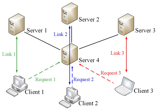
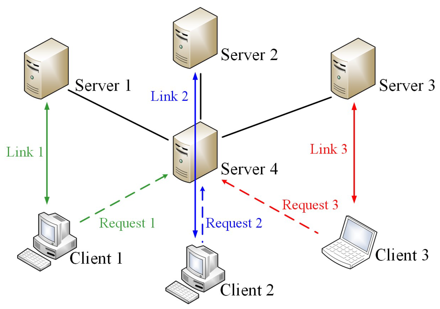
Extending from our previous results as discussed in Section 2, in the following we consider a multi-server system structure as depicted in Figure 1. In this configuration, Server 4 acts as an arbitrator to distribute incoming requests from Clients 1–3 to the assigned Servers 1–3, after which the designated server establishes the direct Links 1–3 with the requester. Beyond ensuring an even distribution of incoming requests, a major goal of this study is to prevent system malfunction or shutdown caused by request overload, while also providing an energy-efficient, power-saving mode for network operation. A novel method is proposed for the arbitrator to fulfill this mission. It consists of two main parts. First, we partition the total server capacity (e.g., maximum service requests) into distinct portions to form upper limits that guide the service load of each server. Second, we construct a switching strategy for efficient load distribution. Details are provided below.

Figure 1. Proposed system structure for communication network.

3.1. Partition of Server Capacity

It is known that the connection number of the server in network service can be treated as “network load”. That is why several existing load balancing schemes have been focused on the balance design of requested connections. For simplicity and without loss of generality, here we adopt the idea of “least connection method” (e.g., [5,6]) to take the connection number of the server for the design. It is not difficult to extend the proposed design to cover other performance indices such as memory utilization and CPU usage of the server by transforming those factors into connection number for practical applications.

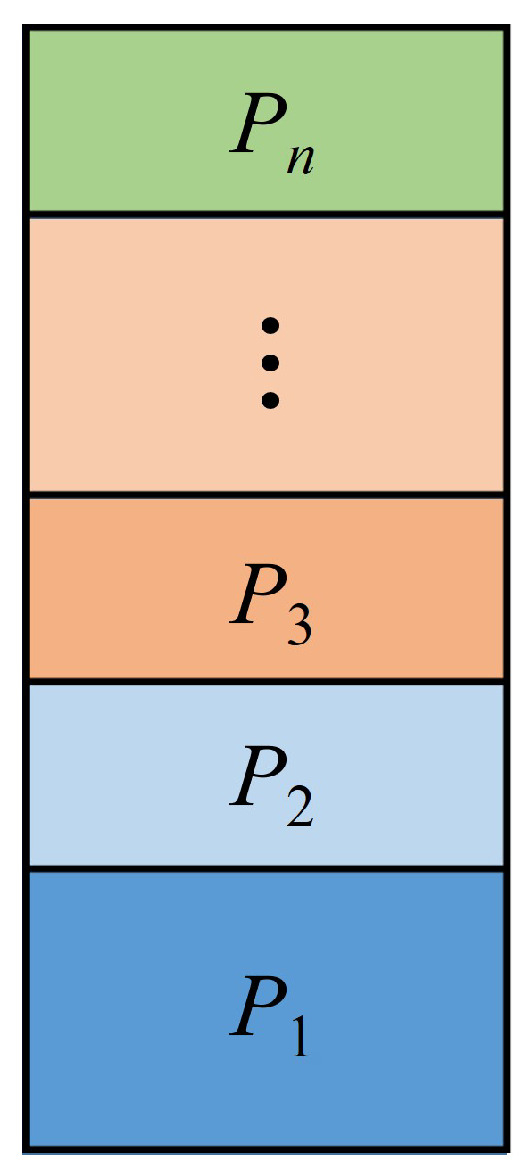
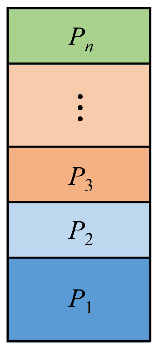
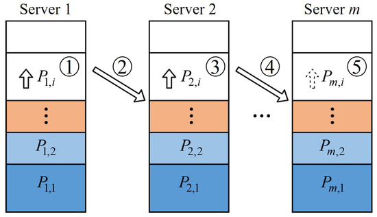
For practical application in multi-server network service, each server would be assigned by the load balancing scheme to serve the incoming requests. Such an assignment might be random. Unlike most of the existing methods, in this study we define the so-called “phase” for the arbitrator to make the decision of the server assignment. In a given phase, each server would have the corresponding amount of capacity as a limit for answering the requested connections. As discussed above, we will take the maximum connection number of the server into account to calculate such a limit. Denote C as the current connection number and $C^{Max}$ as the maximum connection number of the server, respectively. We can then partition the total available connections into n portions, as depicted in Figure 2. As observed in Figure 2, $P_i$ denotes the portion i for $i=1,2,\cdots ,n$. Then we have

$$C^{Max}={\displaystyle \sum _{i=1}^n}{P}_i.$$

(2)

Figure 2. Partition of server capacity.

Let $L^{\left(i\right)}$ be the limit of the connection number of the server in Phase i, for i starting from 1 to a given n. It is clear from Equation (2) above that we can have the following result.

Proposition 1.

The server will not be overloaded if $C\le L^{\left(i\right)}$ for every $i\le n$ with

$$L^{\left(i\right)}={\displaystyle \sum _{j=1}^i}{P}_j.$$

(3)

Remark 1.

Although Proposition 1 provides conditions for preventing the overload of the server, it might not be easy to select the values of n and $P_i$ for $i=1,2,\cdots ,n.$

Instead of finding the method for determining the value of n, in the following we consider an alternative approach for relieving the burden caused by the selection of n. First, let us recall a famous formula in calculating the sum of all the terms in the geometric sequence as Lemma A1 given in Appendix A.

Motivated by Lemma A1, we can choose $P_i={\displaystyle \frac{1}{r^i}}\times C^{Max}$. Here, $r^i$ denotes the exponential function of a positive real number r with the exponent i. Then we have the following result.

Lemma 1.

Let $L^{\left(i\right)}$ be the limit of the connection number of the server in Phase i for i starting from 1 to a given n. Then the server will not be overloaded if $C\le L^{\left(i\right)}$ for any i with $r^j\ge 2$ for all j and

$$L^{\left(i\right)}={\displaystyle \sum _{j=1}^i}{\displaystyle \frac{1}{r^j}}\times C^{Max}.$$

(4)

Proof. 

From Lemma A1, we can rewrite Equation (4) as

$$\begin{array}{ccc}\hfill L^{\left(i\right)}& =& {\displaystyle \frac{C^{Max}}{r}}·{\displaystyle \frac{1-\frac{1}{r^n}}{1-\frac{1}{r}}},\hfill \end{array}$$

(5)

$$\begin{array}{cc} \le & {\displaystyle \frac{C^{Max}}{r}}\times {\displaystyle \frac{1}{1-\frac{1}{r}}},\hfill \end{array}$$

(6)

$$\begin{array}{cc}=& {\displaystyle \frac{C^{Max}}{r-1}}.\hfill \end{array}$$

(7)

It is clear that we have $L^{\left(i\right)}\le C^{Max}$ in any Phase i for $r\ge 2$.    □

Another choice of $P_i$ is to let $P_i={\displaystyle \prod _{j=1}^i}{\displaystyle \frac{1}{r_j}}\times C^{Max}.$ Here, $r_j$ denotes a positive real number. The next result follows readily from Lemma 1.

Lemma 2.

Let $L^{\left(i\right)}$ be the limit of the connection number of the server in Phase i for i starting from 1 to a given n. Then the server will not be overloaded if $C\le L^{\left(i\right)}$ for any i with $r_k\ge 2$ for all k and

$$L^{\left(i\right)}={\displaystyle \sum _{j=1}^i}({\displaystyle \prod _{k=1}^j}{\displaystyle \frac{1}{r_k}}\times C^{Max}).$$

(8)

Remark 2.

The result given in Lemma 1 is a special case of that from Lemma 2.

Two partition methods have been proposed above to prevent the overload of the server. Numerical simulations will be given in Section 4 to combine with the switching strategy proposed in Section 3.2 below for the performance demonstration.

3.2. Switching Strategy

Based on the network structure depicted in Figure 1, Server 4 acts as an arbitrator for distributing all of the incoming requests from clients to the assigned servers. As discussed above, in this study we define the so-called “phase” for the arbitrator to make the decision of the server assignment, i.e., in a given phase each available server would be polled and might be assigned to take care of the current incoming requests by the decision from the arbitrator. In this study, we propose two switching strategies for the arbitrator to select the server for answering the connection requests. One is “normal operation mode” and the other is “power saving mode.” Details are described below.

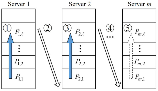
First, we consider the procedure for server assignment in normal operation mode. The objective of this mode is to provide a scheme so that each server will be evenly serving the incoming connection requests without being overloaded. Assume there are m servers available for network service. Let $C_k,C_k^{Max}$ and $L_k^{\left(j\right)}$ denote the current connection number, the maximum connection number and the limit of the connection number of server k in Phase j, respectively. In addition, $P_{k,j}$ denotes the portion of server k in Phase j. To guarantee all of the servers will share the connection requests evenly in each Phase j, the current connection number of every server should be assigned to reach its corresponding limit of Phase j. That is, we will have $C_k=L_k^{\left(j\right)}$ one by one eventually, as denoted by the sequence $\{①,②,\cdots ,⑤\}$ in Figure 3. The phase number will then be increased by one when $C_k=L_k^{\left(j\right)}$ for all $k\in [1,m]$ and the next phase of the server assignment starts to operate.

Figure 3. Switching strategy in normal operation mode.

Based on the discussions above and those given in Section 3.1, we have the following result for guiding the assignment of the server in normal operation mode, as given in Algorithm 1 below.

Algorithm 1 Normal Operation Mode

Step 1.   Construct partition table for $P_{k,j}$ and $L_k^{\left(j\right)}$ by using Lemma 1 or Lemma 2. Step 2.   Let $j=1$ and $k=1$. Step 3.   Input incoming connection request S. Step 4.   Check if $C_k<L_k^{\left(j\right)}$ then assign request S to Server k and go to Step 3. Step 5.   $k=k+1$. Step 6.   Check if $k\le m$ then go to Step 4. Step 7.   Check if $\exists i\in [1,m]$ such that $C_i<L_i^{\left(j\right)}$ then assign request S to Server i and go to Step 11. Step 8.   $j=j+1$ and $k=1$. Step 9.   Check if $j>n^{*}$ then go to Step 12. Step 10. Go to Step 4. Step 11. Input incoming connection request S and go to Step 7. Step 12. Stop.

Remark 3.

It is clear that the portion $P_j$ will become smaller as j becomes large. In the practical application, we will have $P_j=0$ when $j\ge n^{*}$ since the maximum connection number $C^{Max}$ is a finite value. The value $n^{*}$ will then be used as the termination of network service as that in Algorithm 1 above and Algorithm 2 below.

As described in Algorithm 1 and observed in Figure 3, specifically, in Phase 1 each server will be turned on to operate one by one after a different delay time. That means that the proposed scheme can provide a function of power saving for network service.

Next, we consider the procedure for server assignment in power saving mode. Consider, for example, as shown in Table 1 and Table 2, the limit of the connection number of server k in Phase j, as denoted by $L_k^{\left(j\right)}$, can be varied from a small ratio to near one of the maximum connection number $C_k^{Max}$ by properly choosing the value of $r_j$ in the proposed design. Instead of providing a scheme for making each server evenly share the incoming connection requests discussed in the procedure of “normal operation mode,” we will propose a different approach for the operation of power saving, specifically, when the total load of incoming connection requests is not very heavy. Under such a condition, perhaps one or two servers can take care all of the connection requests in a long period of time, as depicted in Figure 4. Extra servers can then be turned on to join the service when the number of total connection requests becomes large.

Table 1. Values of $P_{k,j},L_k^{\left(j\right)}$ and ratio for $C_k^{Max}=1000$ with $r_1=10$ and $r_j=2$ for $j\ge 2$.

Phase	1	2	3	4	5	6	7	$n^{*}$
$r_j$	10	2	2	2	2	2	2	2
$P_{k,j}$	100	50	25	13	6	3	2	1
$L_k^{\left(j\right)}$	100	150	175	188	194	197	199	200
Ratio $(\%)$	10.0	15.0	17.5	18.8	19.4	19.7	19.9	20.0

Table 2. Values of $P_{k,j},L_k^{\left(j\right)}$ and ratio for $C_k^{Max}=1000$ and $r_j=2$ for all j.

Phase	1	2	3	4	5	6	7	8	9	$n^{*}$
$r_j$	2	2	2	2	2	2	2	2	2	2
$P_{k,j}$	500	250	125	63	31	16	8	4	2	1
$L_k^{\left(j\right)}$	500	750	875	938	969	985	993	997	999	1000
Ratio $(\%)$	50.0	75.0	87.5	93.8	96.9	98.5	99.3	99.7	99.9	100.0

Figure 4. Switching strategy in power saving mode.

It is obvious that the performance of power saving depends on the desired ratio $\eta$ of the maximum connection number by proper selection of the phase number ℓ and ratio $r_i$ from the following equation:

$$\eta ={\displaystyle \sum _{j=1}^{\mathsf{\ell }}}({\displaystyle \prod _{i=1}^j}{\displaystyle \frac{1}{r_i}}).$$

(9)

We then have the following algorithm to fulfill the task of power saving.

Algorithm 2 Power Saving Mode

Step 1.   According to the desired power saving ratio $\eta$ of the maximum connection number, solve for Phase ℓ by using Equation (9). Step 2.   Construct partition table for $P_{k,j}$ and $L_k^{\left(j\right)}$ by using the result of Step 1 and Lemma 2. Step 3.   Let k = 1. Step 4.   Input incoming connection request S. Step 5.   Check if $C_k<L_k^{\left(\mathsf{\ell }\right)}$ then assign request S to Server k and go to Step 4. Step 6.   $k=k+1$. Step 7.   Check if $k\le m$ then go to Step 5. Step 8.   Check if $\exists i\in [1,m]$ such that $C_i<L_i^{\left(\mathsf{\ell }\right)}$ then assign request S to Server i and go to Step 17. Step 9.   $j=\mathsf{\ell }+1$ and $k=1$. Step 10. Check if $C_k<L_k^{\left(j\right)}$ then assign request S to Server k and go to Step 18. Step 11. $k=k+1$. Step 12. Check if $k\le m$ then go to Step 10. Step 13. Check if $\exists i\in [1,m]$ such that $C_i<L_i^{\left(j\right)}$ then assign request S to Server i and go to Step 19. Step 14. $j=j+1$ and $k=1$. Step 15. Check if $j>n^{*}$ then go to Step 20. Step 16. Go to Step 10. Step 17. Input incoming connection request S and go to Step 8. Step 18. Input incoming connection request S and go to Step 10. Step 19. Input incoming connection request S and go to Step 13. Step 20. Stop.

4. Simulation Results

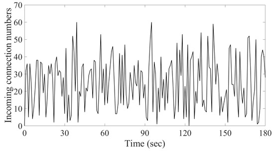
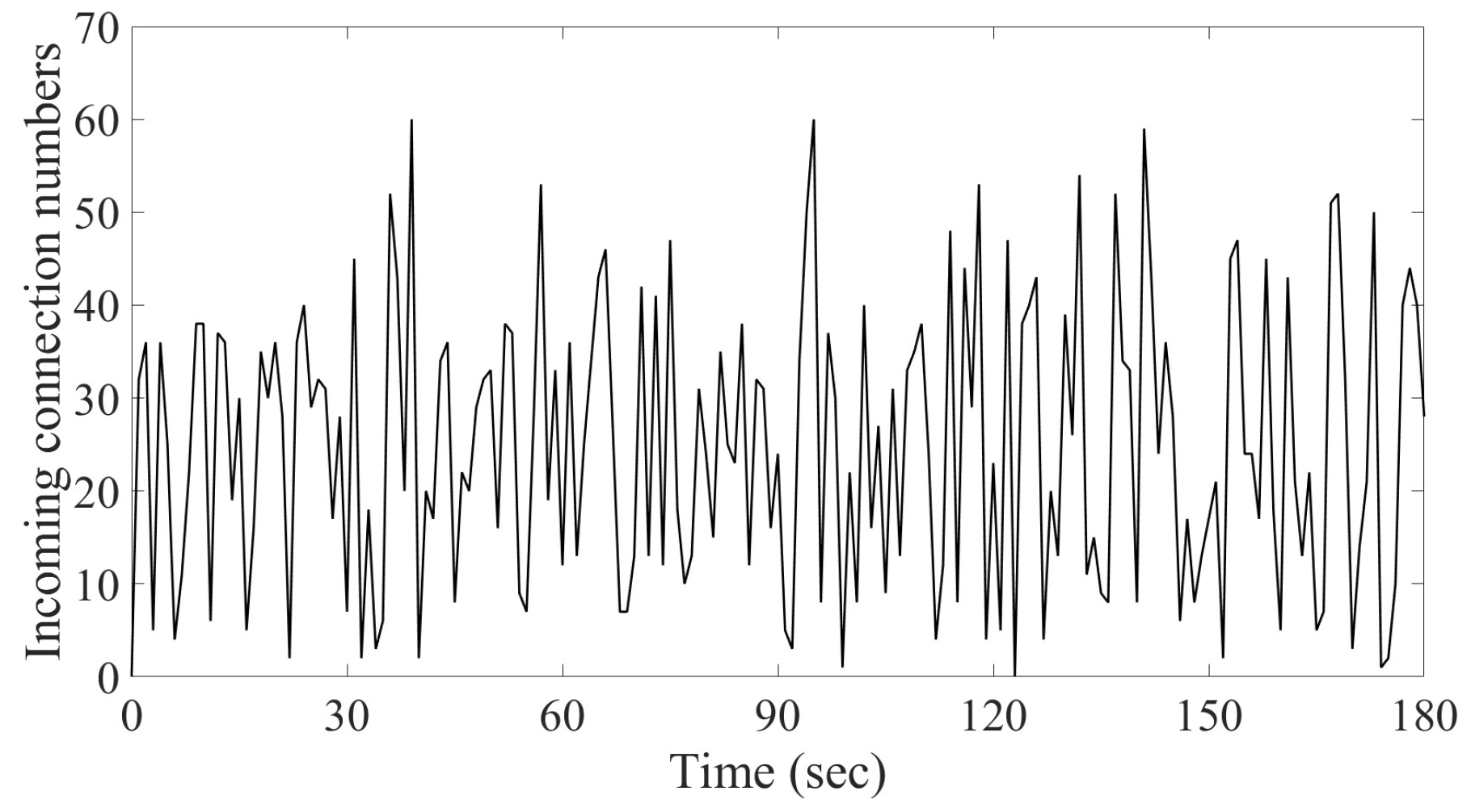
In this section, we will present numerical simulations to demonstrate the usage of Algorithms 1 and 2. This is achieved by using code MATLAB R2024a (e.g., [40]). In order to highlight the difference among the proposed schemes and those existing load balancing methods, three case studies will be discussed. The first one is that the capacities of all available servers are the same for the network service in normal operation mode. It is followed by the case in which the capacities of available servers will be different for the operation in power saving mode. The third case is devoted to the comparison of power consumption for different server structures. For simplicity and without loss of generality, here we consider the case in which three servers are available for network service and the incoming connection requests for three minutes are randomly generated, as depicted in Figure 5. Note that it is not difficult to extend the following study to cover the case of the network for long period of operation with lots of available servers. It is known that least connections and round robin are two of commonly used load balancing algorithms, which stand for dynamic and static types of schemes, respectively. One of the major goals of this paper is to propose a load balancing scheme for the avoidance of server overload. Results from round robin and least connections using Algorithms A1 and A2, given in Appendix A, respectively, will be applied to the comparison of system performance. Details are given as follows.

Figure 5. Incoming connection requests in 3 min.

• Case 1. Same server capacity in normal operation mode

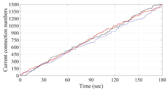
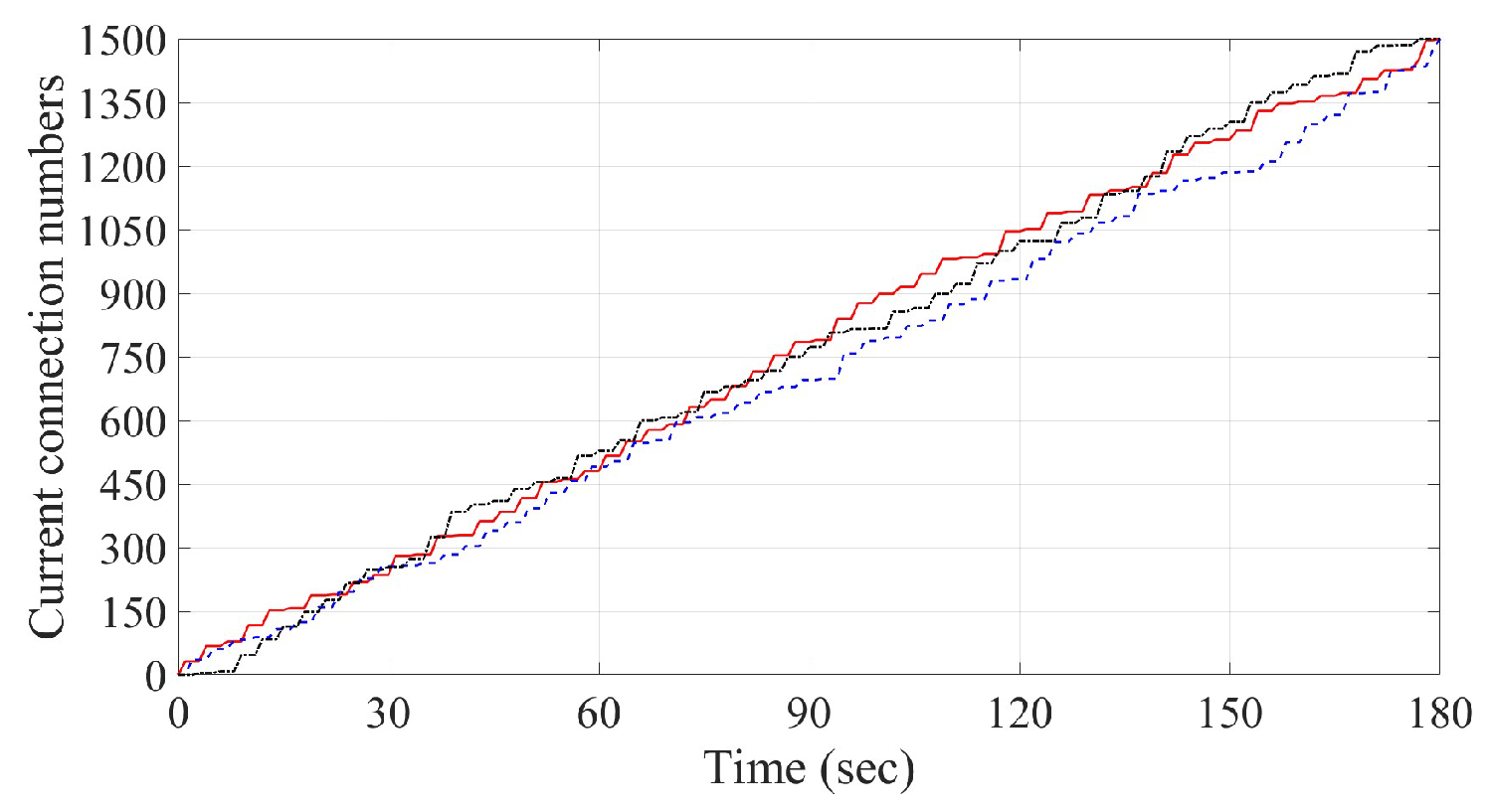
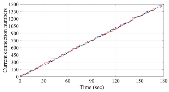
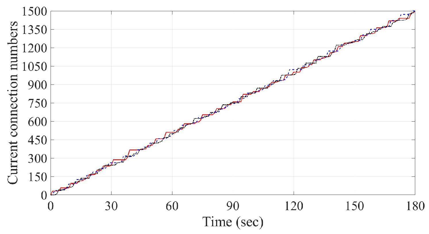
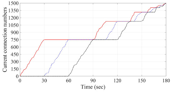
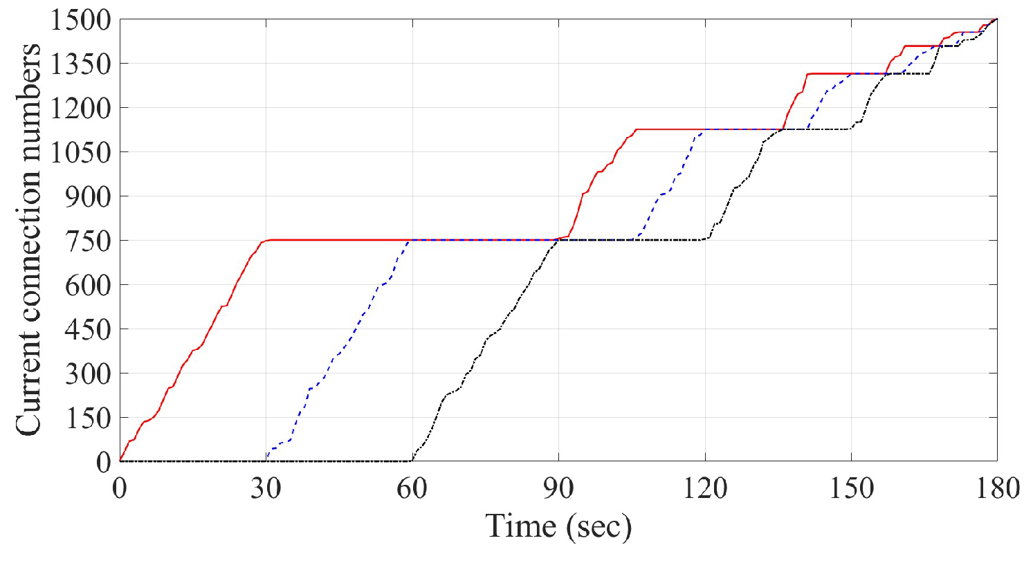
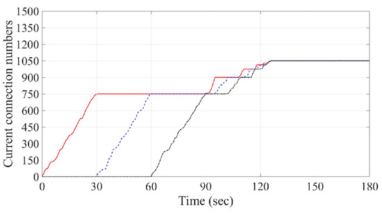
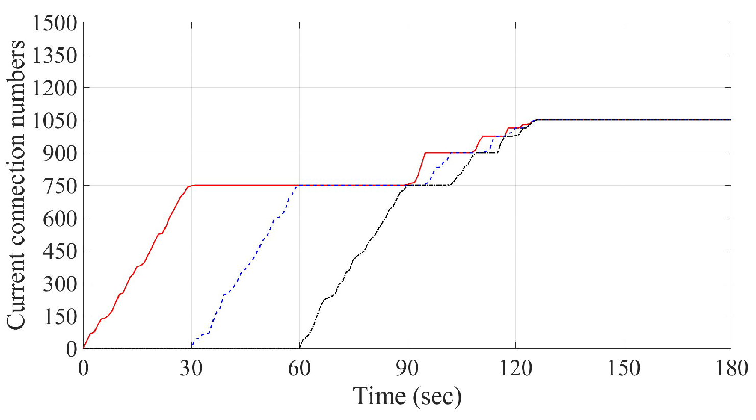
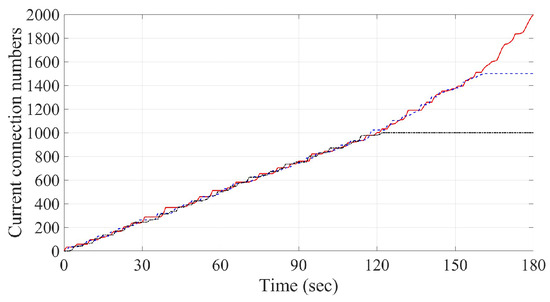
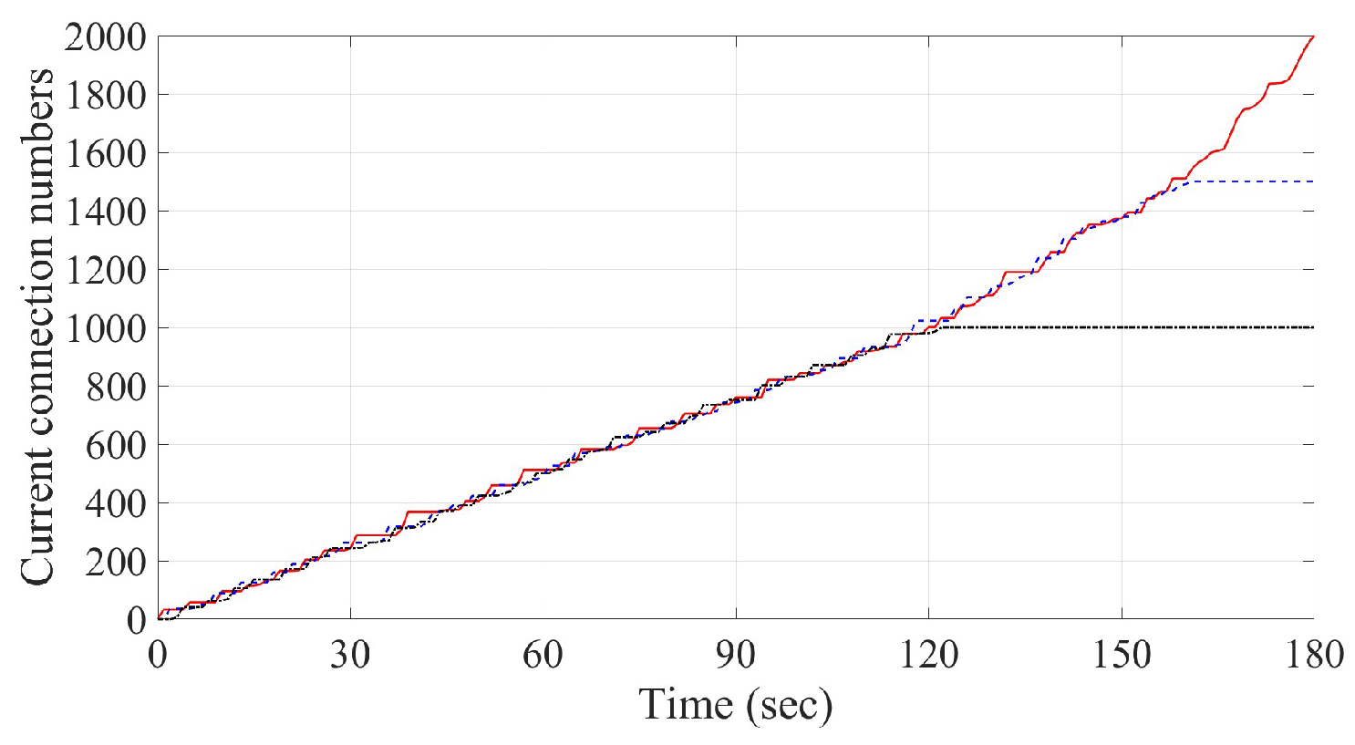
First, we consider the case in which $C_k^{Max}=1500$ for all $k=1,2,3.$ The current connection numbers of three servers using the round robin method are given in Figure 6. As observed in Figure 6, the red line, blue dash-line and black dash-dotted-line denote the connection number for Servers $1,2,3,$ respectively, which will be applied to the numerical simulations presented in this section as those in Figure 7, Figure 8, Figure 9, Figure 10, Figure 11 and Figure 12 below. It is observed from Figure 6 that three curves are staggered together and eventually go to the number of the same maximum capacity. Compared to the above results, the timely distribution of connection requests would be more uniform in three servers by using the least connections mechanism, as shown in Figure 7. Numerical results from Algorithm 1 by using Lemmas 1 and 2 are given in Figure 8 and Figure 9. The corresponding limit $L_k^{\left(j\right)}$ for each k in Phase j is listed in Table 3 and Table 4. As observed from Figure 8 and Figure 9, the current connection number of three servers will eventually and almost simultaneously approach 1500 and 1050, respectively, by the choice of partition. In addition, the incoming connection requests are found to be evenly shared by three servers as the same as those in Figure 6 and Figure 7 by using round robin or least connections. However, there exists a major difference. The starting times for turning on the three servers are almost the same as shown in Figure 6 and Figure 7, while they are different and with time delay one by one, as depicted in Figure 8 and Figure 9.

Figure 6. Current connection numbers of three servers by using round robin method with same server capacity: the red line, blue dash-line and black dash-dotted-line denote the values for Servers $1,2,3,$ respectively.

Figure 7. Current connection numbers of three servers by using least connections method with same server capacity: the red line, blue dash-line and black dash-dotted-line denote the values for Servers $1,2,3,$ respectively.

Figure 8. Current connection numbers of three servers by using Algorithm 1 and Lemma 1: the red line, blue dash-line and black dash-dotted-line denote the values for Servers $1,2,3,$ respectively.

Figure 9. Current connection numbers of three servers by using Algorithm 1 and Lemma 2: the red line, blue dash-line and black dash-dotted-line denote the values for Servers $1,2,3,$ respectively.

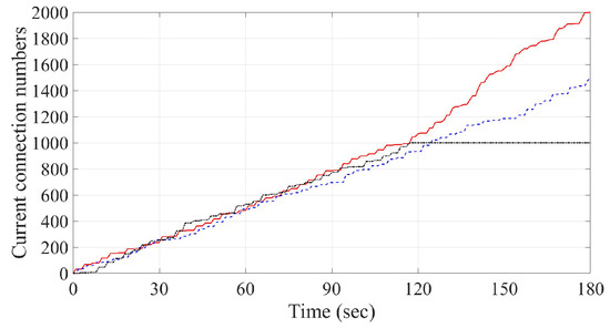
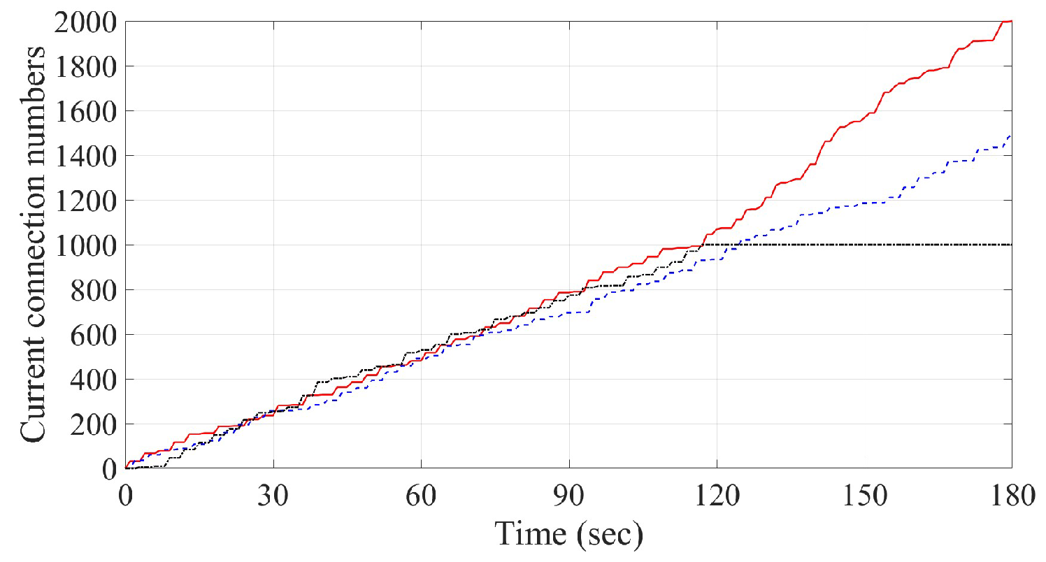
Figure 10. Current connection numbers of three servers by using round robin method with different server capacities: the red line, blue dash-line and black dash-dotted-line denote the values for Servers $1,2,3,$ respectively.

Figure 11. Current connection numbers of three servers by using least connections method with different server capacities: the red line, blue dash-line and black dash-dotted-line denote the values for Servers $1,2,3,$ respectively.

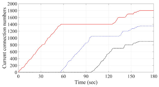
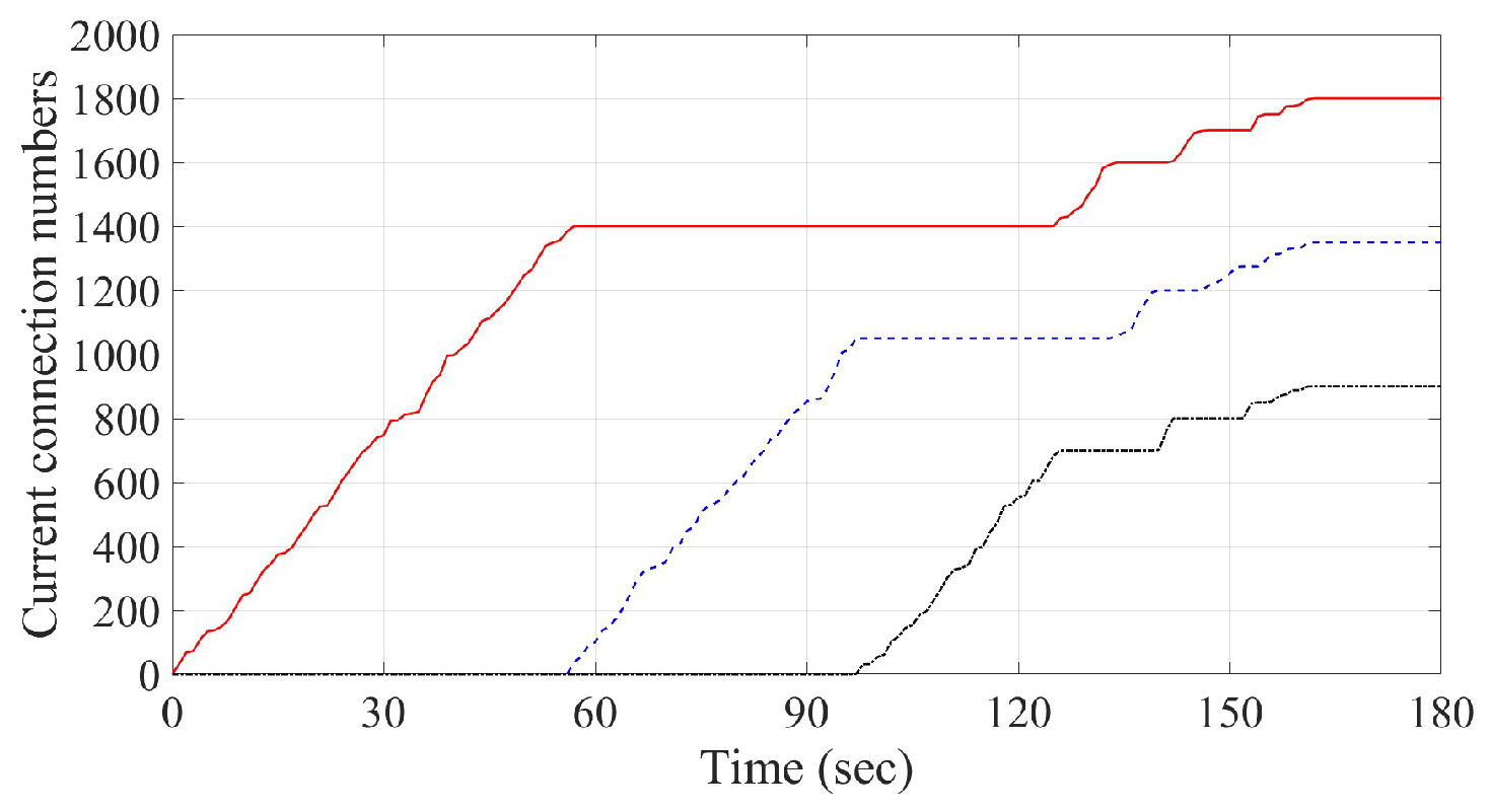
Figure 12. Current connection numbers of three servers by using Algorithm 2 and Lemma 2: the red line, blue dash-line and black dash-dotted-line denote the values for Servers $1,2,3,$ respectively.

Table 3. Values of $L_k^{\left(j\right)}$ for the case of $r_j=2$ for all j.

Phase	1	2	3	4	5	6
Server 1	750	1125	1313	1407	1454	1477
Server 2	750	1125	1313	1407	1454	1477
Server 3	750	1125	1313	1407	1454	1477
Phase	7	8	9	10	$n^{*}$
Server 1	1489	1495	1498	1499	1500
Server 2	1489	1495	1498	1499	1500
Server 3	1489	1495	1498	1499	1500

Table 4. Values of $L_k^{\left(j\right)}$ for the case of $r_2=5$ and $r_j=2$ for all $j\ne 2$.

Phase	1	2	3	4	5	6
Server 1	750	900	975	1013	1032	1041
Server 2	750	900	975	1013	1032	1041
Server 3	750	900	975	1013	1032	1041
Phase	7	8	9	$n^{*}$
Server 1	1046	1048	1049	1050
Server 2	1046	1048	1049	1050
Server 3	1046	1048	1049	1050

• Case 2. Different server capacity in power saving mode

Next, we consider the case of which the maximum capacities of three servers are different. That is, $C_k^{Max}=2000,1500$ and 1000 for $k=1,2,3,$ respectively. Numerical simulations using the round robin method are obtained and shown in Figure 10. Compared to the presentation in Case 1, the connection requests in the simulation by using the least connections algorithm would be more evenly assigned to each server, as depicted in Figure 11. In addition, although three curves in Figure 10 and Figure 11 are initially staggered together, they would eventually one by one go to the number of their different maximum capacities. Simulation results from Algorithm 2 using Lemma 2 for the desired ratio $\eta =70\%$ (with $\mathsf{\ell }=2$ from Equation (9)) are given in Figure 12. The corresponding limits $L_k^{\left(j\right)}$ for each k in Phase j are listed in Table 5. It is observed from Figure 12 that the current connection number of the three servers will eventually and almost simultaneously approach 1800, 1350 and 900, respectively. Furthermore, the incoming connection requests are also found to be evenly shared by the three servers. Compared with the design of normal operation mode, the procedure of power saving mode can provide bigger time delay for the starting time of the next server to operate, as depicted in Figure 8 and Figure 12. However, the allowable maximum connection number will be decreased in power saving mode, as listed in Table 5 and depicted in Figure 12. To check with the flow of Algorithms 1 and 2, the procedure of server assignment starts from Server 1, then checking the next available server. It is clear from Figure 12 that the server with bigger maximum connection number should be assigned a lower number to provide longer delay time for power saving as those servers defined in this case. That is, in the study of Case 2 we have $C_k^{Max}=2000,1500$ and 1000 for $k=1,2,3,$ respectively, to provide longer delay time for power saving.

Table 5. Values of $L_k^{\left(j\right)}$ for the case of servers’ capacity being different.

Phase	1	2 $\left(\mathsf{\ell }\right)$	3	4	5	6
Server 1	1000	1400	1600	1700	1750	1775
Server 2	750	1050	1200	1275	1313	1332
Server 3	500	700	800	850	875	888
Phase	7	8	9	10	$n^{*}$
Server 1	1788	1794	1797	1799	1800
Server 2	1341	1346	1348	1349	1350
Server 3	894	897	899	900	900

• Case 3. Comparison of energy consumption

As presented in Cases 1 and 2 above, we have successfully demonstrated the results of preventing the occurrence of server overload by using Algorithms 1 and 2. In the following, we will study the performance of energy consumption by using the proposed energy-saving scheme under the two different server structures, as discussed in Cases 1 and 2. Among those existing studies [41,42,43] of server power consumption, a simple method is proposed to estimate and calculate the total system energy consumption of the server [41]. Such a model is adopted below to demonstrate the performance comparison of energy consumption by using round robin algorithm, least connections algorithm and the proposed scheme, as given in Algorithm 2, respectively. The power model proposed in [41] is recalled as below:

$$P_{total}=P_{idle}+(P_{busy}-P_{idle})(2u-u^{\gamma })$$

(10)

where $P_{total}$, $P_{idle}$, $P_{busy}$, u and $\gamma$ denote current power consumption, idle power consumption, full loading power consumption, CPU utilization and a constant value, respectively.

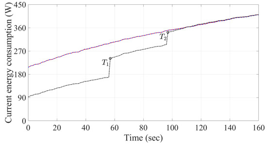
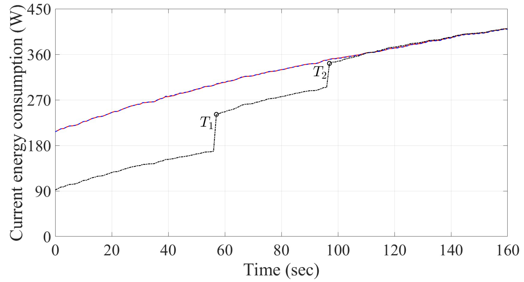
In this study, we choose parameter $\gamma =1.4$ from [41] and the variable u is related to incoming connection requests for each server. Furthermore, in the following numerical study (referring to [43]), the values of $P_{idle}$ and $P_{busy}$ for $C_k^{Max}=1500$ are set as 69 W and 142 W, respectively. Based on the power model recalled above, we can calculate the power consumption of each server under the two server structures defined in Cases 1 and 2. The maximum capacities of three servers in Case 1 have the same value of $C_k^{Max}=1500$, while the maximum capacities of the three servers in Case 2 are $C_k^{Max}=2000,1500$ and 1000 for $k=1,2,3,$ respectively. Due to the limitation of phase, as shown in Figure 12, we only calculate the power consumption from 0 to 160 s.

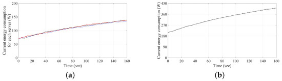
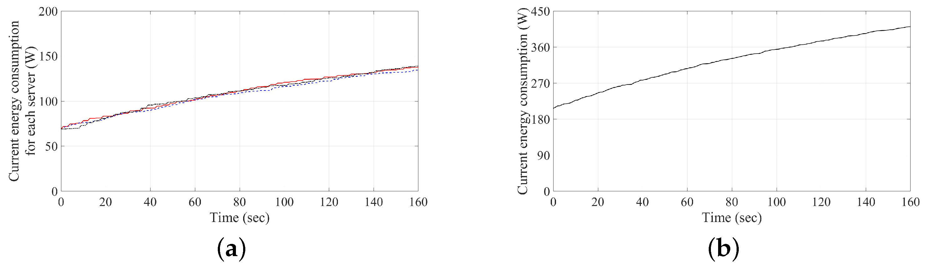
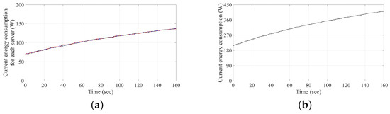
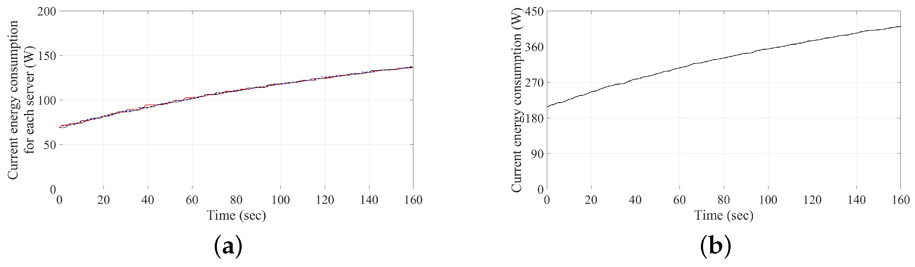
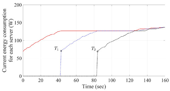
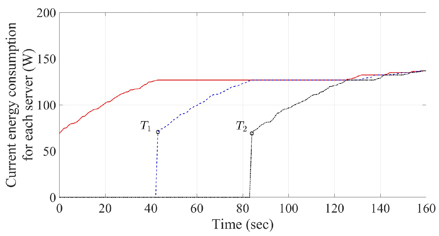
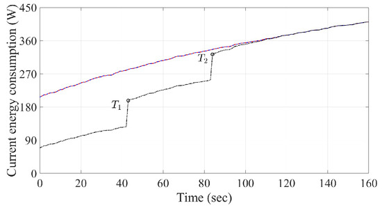
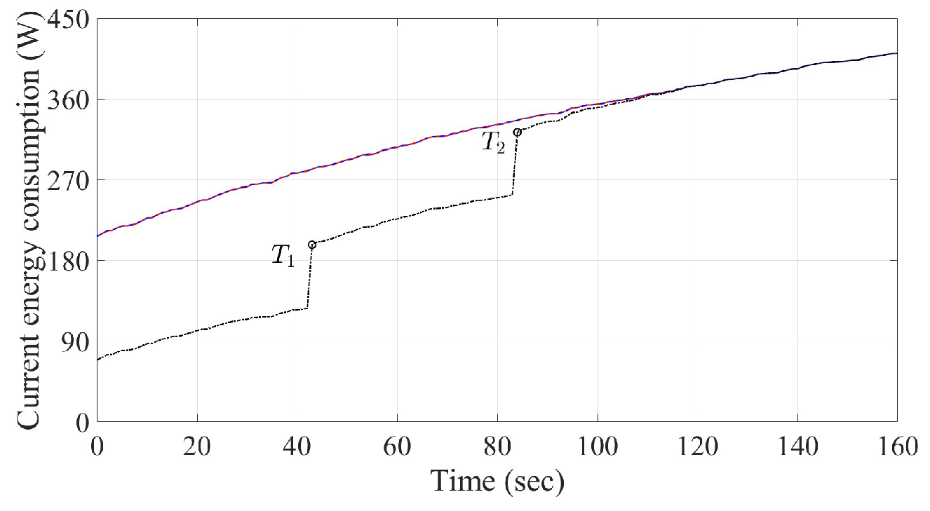
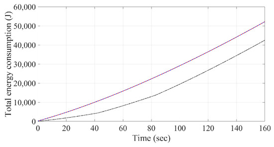
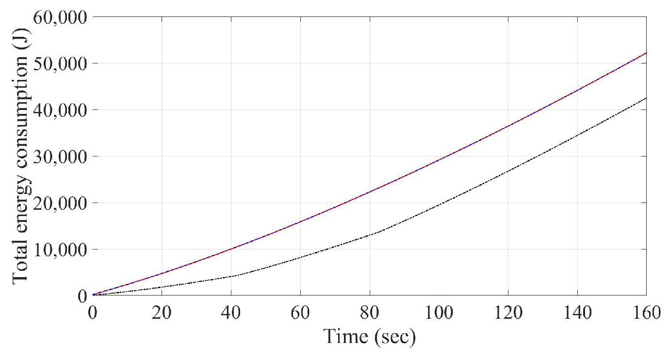
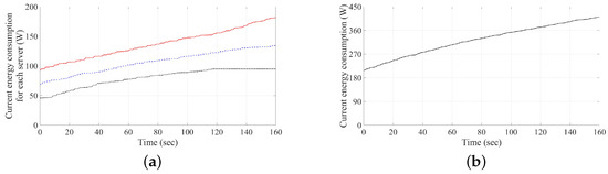
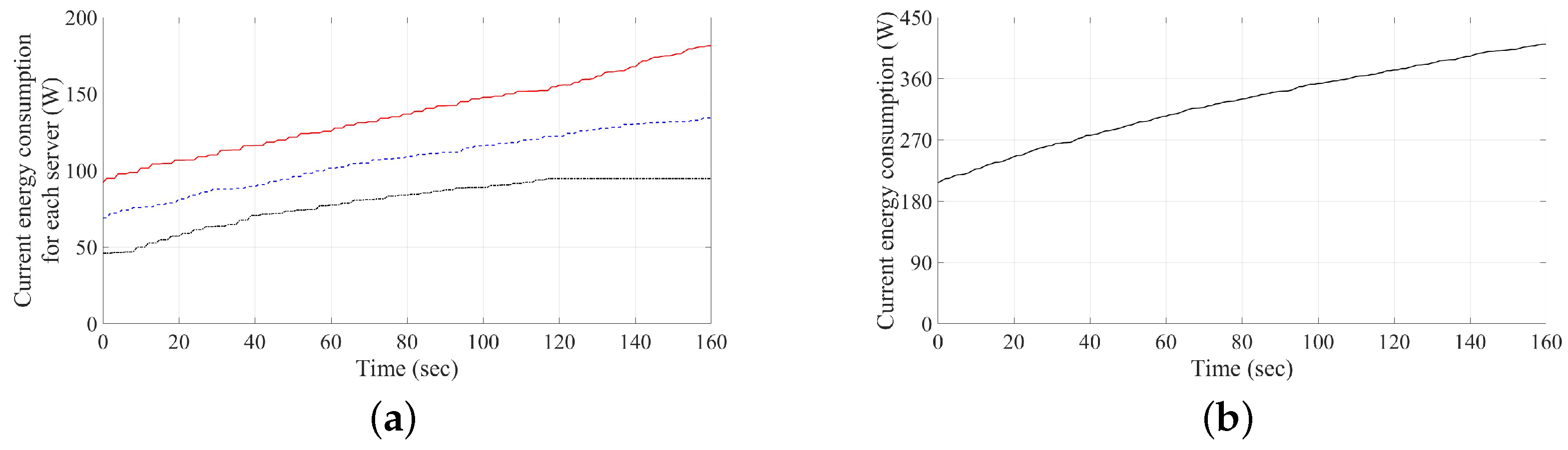
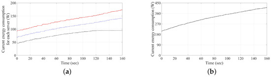
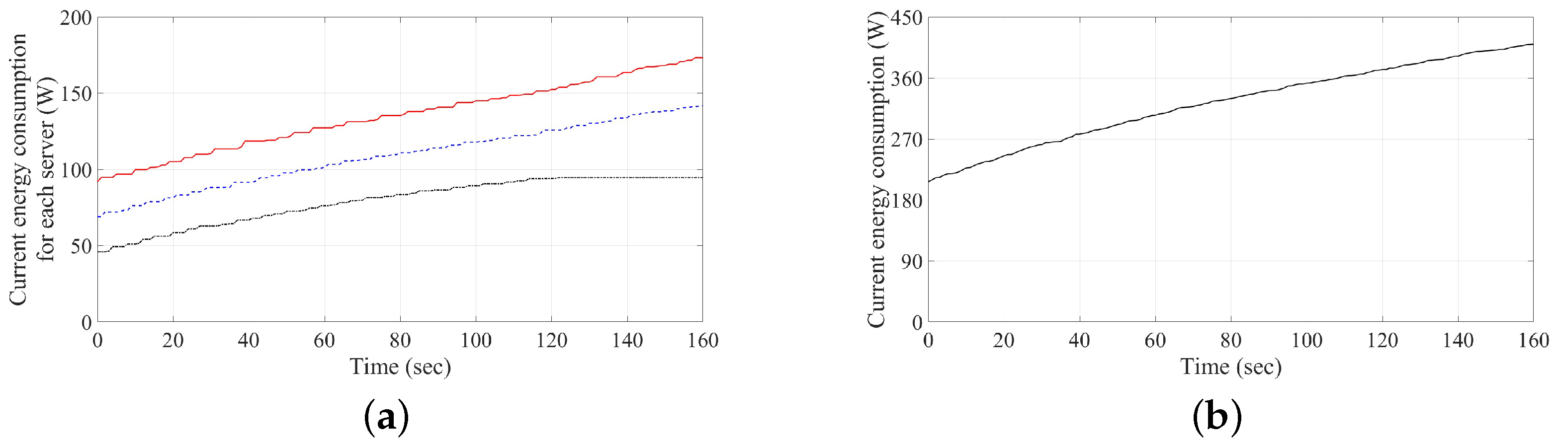
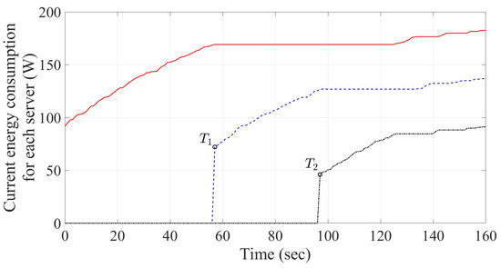
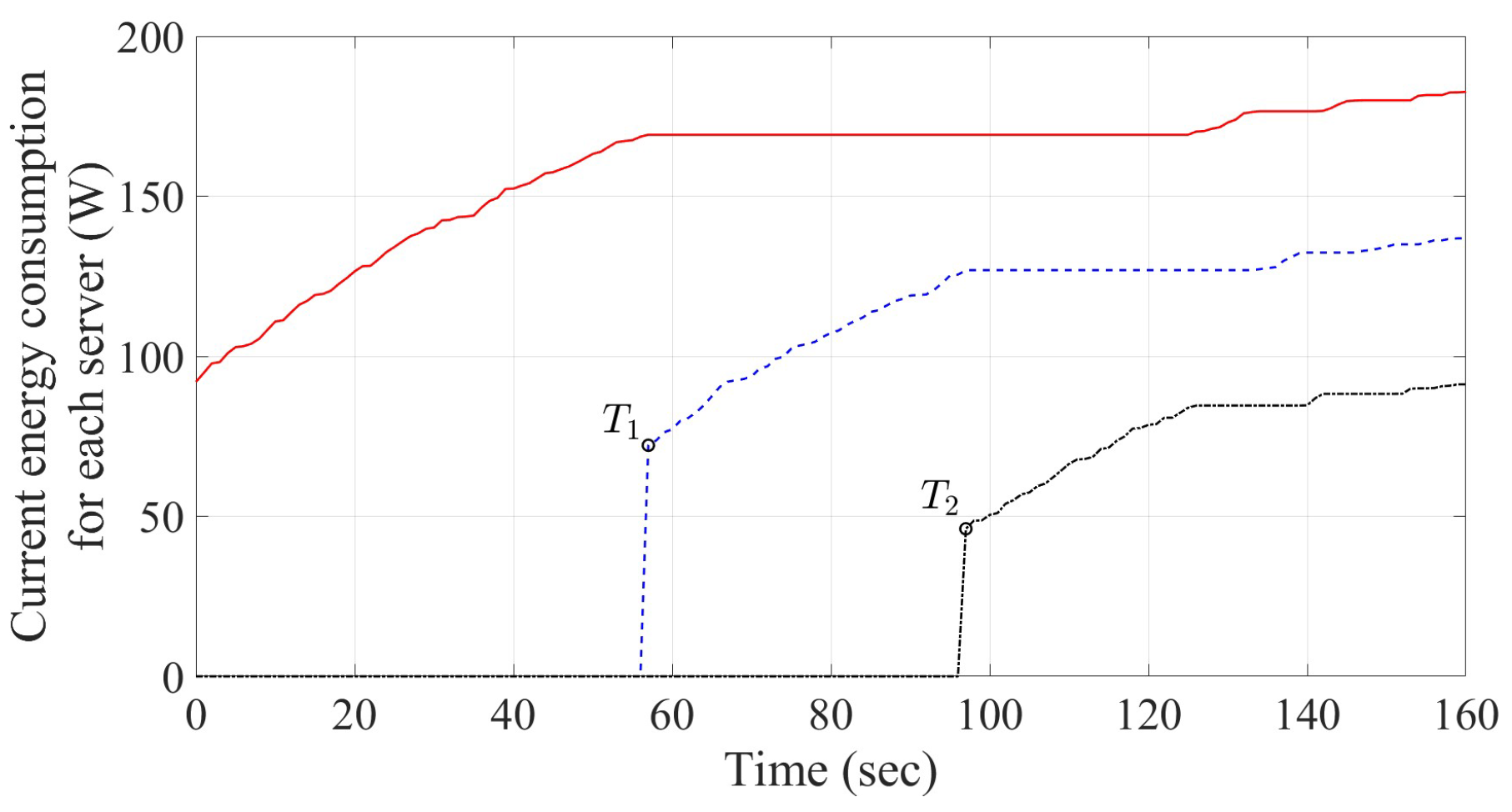
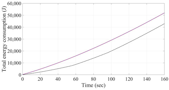
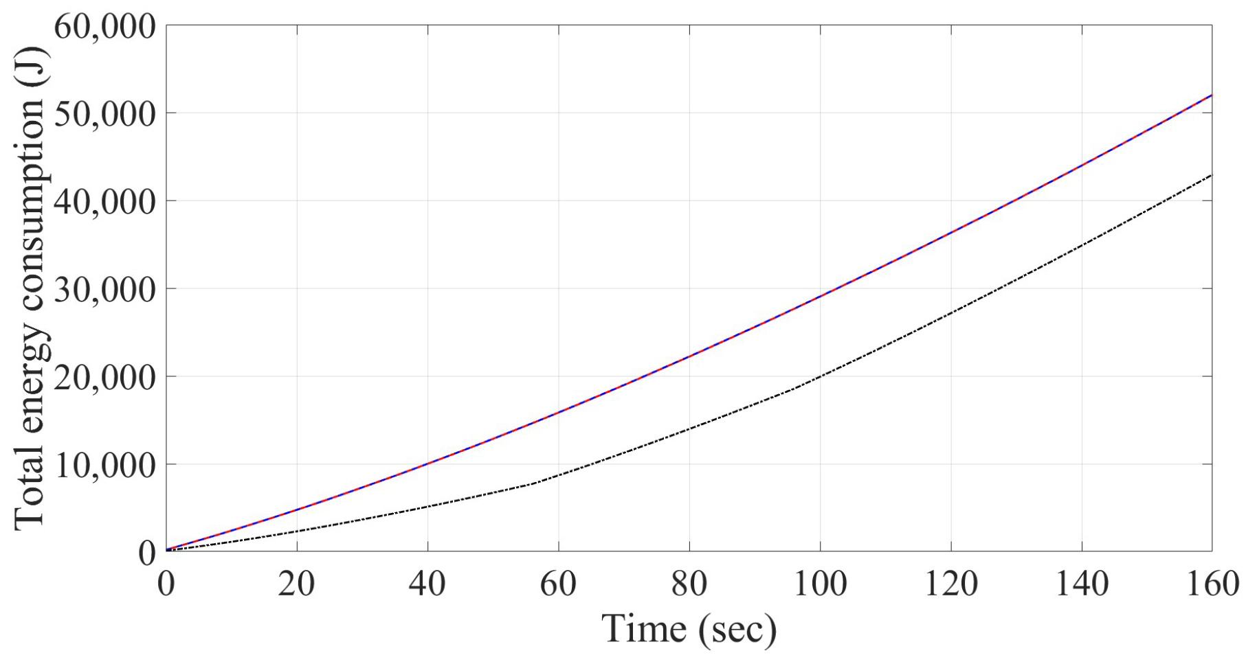
First, we consider the server structure defined in Case 1. Based on the values discussed above, the power model recalled in Equation (10) is used for calculating current energy consumptions of each server using the round robin method, least connections method and Algorithm 2, respectively, as depicted in Figure 13, Figure 14 and Figure 15. As shown in Figure 13a, the red line, blue dash-line and black dash-dotted-line denote the energy consumption for servers $1,2,3,$ respectively, which will be applied to the numerical simulations presented in this section as those in Figure 14a and Figure 15 below. In addition, the black curve denotes the summation of the three current servers’ energy consumption, as shown in Figure 13b, which, of these definitions, will also be used in Figure 14b below. Moreover, the sum of current energy consumption from three servers and the cumulative of total energy consumption by three load balancing schemes are also obtained as depicted in Figure 16 and Figure 17 for the performance comparison. In Figure 16 and Figure 17, the red line, blue dash-line and black dash-dotted-line denote the values by using round robin, least connections and Algorithm 2, respectively. As observed in Figure 13a and Figure 14a, incoming connection requests would almost be evenly and smoothly distributed to three servers at the starting time due to the mechanism frameworks, as described in Algorithms A1 and A2. The sums of current energy consumption of three servers in the numerical simulations by using two algorithms are also found to be smoothly and evenly added on, as those given in Figure 13b and Figure 14b. Instead, Servers 2 and 3 are turned on at time $T_1=43$ s and $T_2=84$ s, as shown in Figure 15, respectively, while using Algorithm 2. It can be clearly observed in Figure 16 that the summation of the current three servers’ energy consumption using Algorithm 2 would be even less than the other two methods before the time instant $T_2$. The cumulative total energy consumption of the three schemes is depicted in Figure 17, which provides the evidence of power saving using the proposed algorithm for load balancing. Note that the cumulative total energy consumption using the round robin algorithm, least connections algorithm and Algorithm 2 at time $t=160$ are obtained as 52,194.2 J, 52,201.5 J and 42,509.6 J, respectively.

Figure 13. Current energy consumption using round robin method under the structure of Case 1: (a) current energy consumption for each server (the red line, blue dash-line and black dash-dotted-line denote the values for servers $1,2,3,$ respectively) and (b) summation of three current servers’ energy consumption.

Figure 14. Current energy consumption by using least connections method under the structure of Case 1: (a) Current energy consumption for each server (the red line, blue dash-line and black dash-dotted-line denote the values for servers $1,2,3,$ respectively) and (b) Summation of three current servers’ energy consumption.

Figure 15. Current energy consumption for each server using Algorithm 2 under the structure of Case 1: the red line, blue dash-line and black dash-dotted-line denote the values for servers $1,2,3,$ respectively. The turned on time for Servers 2 and 3 are both $T_1=43$ s and $T_2=84$ s.

Figure 16. Summation of three current servers’ energy consumption under the structure of Case 1: the red line, blue dash-line and black dash-dotted-line denote the values for servers $1,2,3,$ respectively. The turned on time for Servers 2 and 3 are both $T_1=43$ s and $T_2=84$ s.

Figure 17. Cumulative total energy consumption under the structure of Case 1 in $t=0$–160: the red line, blue dash-line and black dash-dotted-line denote the values for servers $1,2,3,$ respectively.

Next, we consider the server structure defined in Case 2. In this case, the three servers have different maximum affordable power consumption of 189.3 W, 142 W and 94.7 W for Server 1, Server 2 and Server 3, respectively. The idle power consumption for the three servers also comprises different values of 92 W, 69 W and 46 W. Similarly, the current energy consumptions of each server using round robin, least connections and Algorithm 2 are depicted in Figure 18, Figure 19 and Figure 20, respectively. In addition, the sum of current energy consumption from three servers and the cumulative total energy consumption by three load balancing schemes are also obtained as shown in Figure 21 and Figure 22. As depicted in Figure 18a, the red line, blue dash-line and black dash-dotted-line denote the energy consumption for servers $1,2,3,$ respectively, which will be applied to the numerical simulations presented in this section as those in Figure 19a, and Figure 20 below. In addition, the black curve denotes the summation of the three current servers’ energy consumption, as shown in Figure 18b, which, of these definitions, will also be used in Figure 19b. Moreover, In Figure 21 and Figure 22, the red line, blue dash-line and black dash-dotted-line denote the values by using round robin, least connections and Algorithm 2, respectively. Compared with the results as given in Figure 13, Figure 14, Figure 15, Figure 16 and Figure 17, it is obvious to see the benefit of power saving in our proposal from Figure 18, Figure 19, Figure 20, Figure 21 and Figure 22. Furthermore, it is observed from Figure 20 and Figure 21 that Server 2 and Server 3 are turned on at times $T_1=57$ s and $T_2=97$ s, respectively, using Algorithm 2. The cumulative total energy consumption using the round robin algorithm, least connections algorithm and Algorithm 2 at time $t=160$ is obtained as 52,014.7 J, 51,997.6 J and 42,917 J, respectively, which justifies the function of power saving that can be achieved using the proposed algorithm for load balancing.

Figure 18. Current energy consumption using round robin method under the structure of Case 2: (a) current energy consumption for each server (the red line, blue dash-line and black dash-dotted-line denote the values for servers $1,2,3,$ respectively) and (b) summation of three current servers’ energy consumption.

Figure 19. Current energy consumption using least connections method under the structure of Case 2: (a) current energy consumption for each server (the red line, blue dash-line and black dash-dotted-line denote the values for servers $1,2,3,$ respectively) and (b) summation of three current servers’ energy consumption.

Figure 20. Current energy consumption for each server using Algorithm 2 under the structure of Case 2: the red line, blue dash-line and black dash-dotted-line denote the values for servers $1,2,3,$ respectively. The turned on time for Servers 2 and 3 are both $T_1=57$ s and $T_2=97$ s.

Figure 21. Summation of three current servers’ energy consumption under the structure of Case 2: the red line, blue dash-line and black dash-dotted-line denote the values for servers $1,2,3,$ respectively. The turned on time for Servers 2 and 3 are both $T_1=57$ s and $T_2=97$ s.

Figure 22. Cumulative total energy consumption under the structure of Case 2 in $t=0$–160: the red line, blue dash-line and black dash-dotted-line denote the values for servers $1,2,3,$ respectively.

Note that, as recalled in the Introduction, several commercial network service platforms have been developed to perform the function of load balancing or load distribution with and without dynamically changing the total amount of serving machines to fulfill the task of the so-called “scalability” for the multi-server system (e.g., [10,11,12,13,14]). It is clear from the numerical results above that such a function can also be achieved by using the proposed power-saving schemes.

5. Discussion

It is known that distributing server load is critical in multi-server environments. Most studies, as recalled in Section 1 and Section 2, focus on developing load balancing schemes to distribute load evenly across all available servers over time. In contrast to these existing schemes, this study proposes a different approach: a load distribution method designed to provide energy-efficient service and prevent the occurrence of overload.

In this study, our previous works [31,32] provide the technical foundation for constructing the “capacity partition” in Section 3.1. This ensures that the accumulated total partition of service capacity does not exceed its maximum value, thereby preventing overload. Based on this scheme, two switching algorithms—Algorithms 1 and 2—are proposed in Section 3.2 for normal and power-saving operations. A comparative study with Least Connection and Round Robin schemes in Section 4 has demonstrated the superiority of the proposed design. Furthermore, compared to the studies reviewed in Section 2, our scheme achieves energy efficiency more simply, without the need for time-consuming optimization as required in, e.g., [27,33,34,35,36].

In this paper, we assume the communication network structure is an arbitrator-based platform, as shown in Figure 1, where Server 4 acts as the arbitrator. Based on this service structure, a practical application scenario is as follows. The partition table for all available servers (as illustrated in one of the five tables, Table 1, Table 2, Table 3, Table 4 and Table 5) is stored exclusively at the arbitrator rather than at the individual servers. The load distribution, as described in Algorithm 1 or Algorithm 2, is then performed by the arbitrator. According to these algorithms, real-time monitoring of each server’s remaining capacity is unnecessary. Instead, such actions only occur during the switching phase, as specified in Step 7 of Algorithm 1 and Step 8 of Algorithm 2. Compared to the threshold-based algorithms in [7,19,20,39], this design can relax the communication burden between the arbitrator and each server.

In the two proposed algorithms (Algorithms 1 and 2), the total number of available servers is denoted by “m” and the total number of switching phases by “$n^{*}$”. These two parameters play crucial roles in practical load distribution and are determined by the system designer. Based on the values of m and $n^{*}$, the arbitrator constructs a partition table to execute the algorithm, with termination conditions defined in Step 9 of Algorithm 1 and Step 15 of Algorithm 2. As demonstrated in Section 4, the power-saving mode does not distribute the load evenly across all servers throughout the entire timeline. Instead, the proposed design mitigates the energy burden of idle power consumption by activating servers only when additional service capacity is required. Consequently, the functionality of scalability (e.g., [10,11,12,13,14]) or auto-scaling (e.g., [26,27,30,37,38]) can then be achieved by applying Algorithm 2 with a dynamically adjusted value of m.

6. Conclusions

The issue of server load distribution scheme is known to be crucial and substantial in multi-server network service. In this study, we have proposed a novel scheme which can prevent overloading and ensure load balancing. Additionally, this scheme enhances system scalability by utilizing a power-saving mode to dynamically add or remove servers. While simulation results demonstrate the design’s effectiveness, the impact of different service capacity definitions on performance remains unexplored and will be addressed in future work.

References

- Kumar, C.; Marston, S.; Sen, R.; Narisetty, A. Greening the cloud: A load balancing mechanism to optimize cloud computing networks. J. Manag. Inform. Syst. 2022, 39, 513–541. [Google Scholar] [CrossRef] [Scilit]
- Furqan, M.; Ali, Z.; Jan, Q.; Nazir, S.; Iqbal, S.; Huang, Y. An efficient load-balancing scheme for UAVs in 5G infrastructure. IEEE Syst. J. 2023, 17, 780–791. [Google Scholar] [CrossRef] [Scilit]
- Shi, Y.; Yang, Q.; Huang, X.; Li, D.; Huang, X. An SDN-enabled framework for a load-balanced and QoS-aware internet of underwater things. IEEE Internet Things J. 2023, 10, 7824–7834. [Google Scholar] [CrossRef] [Scilit]
- Arshiya; Singh, J. Genetic approach based optimized load balancing in cloud computing: A performance perspective. In Proceedings of the 2022 9th International Conference on Computing for Sustainable Global Development (INDIACom), New Delhi, India, 23–25 March 2022; IEEE: New York, NY, USA, 2022; pp. 814–819. [Google Scholar]
- Harjanti, T.W.; Setiyani, H.; Trianto, J. Load balancing analysis using round-robin and least-connection algorithms for server service response time. Appl. Technol. Comput. Sci. J. 2022, 5, 40–49. [Google Scholar] [CrossRef] [Scilit]
- Rahmika, A.R.; Tahir, Z.; Paundu, A.W.; Zainuddin, Z. Web server load balancing mechanism with least connection algorithm and multi-agent system. CommIT J. 2023, 17, 245–258. [Google Scholar] [CrossRef] [Scilit]
- Singh, G.; Kaur, K. An improved weighted least connection scheduling algorithm for load balancing in web cluster systems. Int. Res. J. Eng. Technol. 2018, 5, 1950–1955. [Google Scholar]
- Bourke, T. Server Load Balancing, 1st ed.; O’Reilly: Sebastopol, CA, USA, 2001. [Google Scholar]
- Shafiq, D.A.; Jhanjhi, N.Z.; Abdullah, A. Load balancing techniques in cloud computing environment: A review. J. King Saud. Univ. Comput. Inf. Sci. 2022, 34, 3910–3933. [Google Scholar] [CrossRef] [Scilit]
- Tencent Cloud, Cloud Load Balancer. Available online: https://www.tencentcloud.com/pt/products/clb (accessed on 6 March 2026).
- Genesys Engage, Load Distribution Server. Available online: https://docs.genesys.com/Documentation/LDS (accessed on 6 March 2026).
- f5, What Is a Load Balancer? Available online: https://www.f5.com/glossary/load-balancer (accessed on 6 March 2026).
- AWS, Network Load Balancers. Available online: https://docs.aws.amazon.com/elasticloadbalancing/latest/network/network-load-balancers.html (accessed on 6 March 2026).
- Microsoft, Azure Load Balancer. Available online: https://azure.microsoft.com/en-us/products/load-balancer/ (accessed on 6 March 2026).
- Alam, M.; Khan, Z.A. Issues and challenges of load balancing algorithm in cloud computing environment. Indian J. Sci. Technol. 2017, 10, 1–12. [Google Scholar] [CrossRef] [Scilit]
- Patel, G.; Mehta, R.; Bhoi, U. Enhanced load balanced min-min algorithm for static meta task scheduling in cloud computing. Procedia Comput. Sci. 2015, 57, 545–553. [Google Scholar] [CrossRef] [Scilit]
- Sarddar, D.; Chakraborty, S.; Roy, M. An efficient approach to calculate dynamic time quantum in round robin algorithm for efficient load balancing. Int. J. Comput. Appl. 2015, 123, 48–52. [Google Scholar] [CrossRef] [Scilit]
- Anselmi, J. Combining size-based load balancing with round-robin for scalable low latency. IEEE Trans. Parallell Distr. 2020, 31, 886–896. [Google Scholar] [CrossRef] [Scilit]
- Katangur, A.; Akkaladevi, S.; Vivekanandhan, S. Priority weighted round robin algorithm for load balancing in the cloud. In Proceedings of the 2022 IEEE 7th International Conference on Smart Cloud (SmartCloud), Shanghai, China, 8–10 October 2022; IEEE: New York, NY, USA, 2022; pp. 230–235. [Google Scholar]
- Priya, D.S.; Perumal, S. An integrated algorithm for load balancing discrepancies in cloud computing using weighted least connection. In Proceedings of the 2024 International Conference on Innovative Computing, Intelligent Communication and Smart Electrical Systems (ICSES), Chennai, India, 12–13 December 2024; IEEE: New York, NY, USA, 2024; pp. 1–7. [Google Scholar]
- Zhu, L.; Cui, J.; Xiong, G. Improved dynamic load balancing algorithm based on least-connection scheduling. In Proceedings of the 2018 IEEE 4th Information Technology and Mechatronics Engineering Conference (ITOEC), Chongqing, China, 14–16 December 2018; IEEE: New York, NY, USA, 2018; pp. 1858–1862. [Google Scholar]
- Liu, C.; Li, K.; Li, K. A game approach to multi-servers load balancing with load-dependent server availability consideration. IEEE Trans. Cloud Comput. 2021, 9, 1–13. [Google Scholar] [CrossRef] [Scilit]
- Chen, X.; Yao, Z.; Chen, Z.; Min, G.; Zheng, X.; Rong, C. Load balancing for multiedge collaboration in wireless metropolitan area networks: A two-stage decision-making approach. IEEE Internet Things J. 2023, 10, 17124–17136. [Google Scholar] [CrossRef] [Scilit]
- Jasim, A.M.; Al-Raweshidy, H. An adaptive SDN-based load balancing method for edge/fog-based real-time healthcare systems. IEEE Syst. J. 2024, 18, 1139–1150. [Google Scholar] [CrossRef] [Scilit]
- Cao, J.; Li, K.; Stojmenovic, I. Optimal power allocation and load distribution for multiple heterogeneous multicore server processors across clouds and data centers. IEEE Trans. Comput. 2014, 63, 45–58. [Google Scholar]
- Ayaz, Z.; Yüksel, M.E. A rule-based server activation strategy for dynamic load balancing and energy efficiency in data centers. Adv. Theory Simul. 2025, 8, e00838. [Google Scholar] [CrossRef] [Scilit]
- Forghani, M.; Soltanaghaei, M.; Boroujeni, F.Z. Dynamic optimization scheme for load balancing and energy efficiency in software-defined networks utilizing the krill herd meta-heuristic algorithm. Comput. Electr. Eng. 2024, 114, 109057. [Google Scholar] [CrossRef] [Scilit]
- Khaleghzadeh, H.; Fahad, M.; Shahid, A.; Manumachu, R.R.; Lastovetsky, A. Bi-objective optimization of data-parallel applications on heterogeneous HPC platforms for performance and energy through workload distribution. IEEE Trans. Parallel Distrib. Syst. 2021, 32, 543–560. [Google Scholar] [CrossRef] [Scilit]
- Khaleghzadeh, H.; Fahad, M.; Manumachu, R.R.; Lastovetsky, A. A novel data partitioning algorithm for dynamic energy optimization on heterogeneous high-performance computing platforms. Concurr. Comput. Pract. Exp. 2020, 32, e5928. [Google Scholar] [CrossRef] [Scilit]
- Priyadarsini, M.; Kumar, S.; Bera, P.; Rahman, M.A. An energy-efficient load distribution framework for SDN controllers. Computing 2020, 102, 2073–2098. [Google Scholar] [CrossRef] [Scilit]
- Liaw, D.-C.; Yeh, C.-W.; Chiu, C.-H.; Chang, C.-M.; Hsieh, H.-J. A load balancing scheme for web server design. In Proceedings of the 2011 International Conference on System Science and Engineering, Macau, China, 8–10 June 2011; IEEE: New York, NY, USA, 2011; pp. 32–36. [Google Scholar]
- Liaw, D.-C. Method for Load Distribution. ROC Patent No. TW I414161 B, 1 November 2013. (In Chinese) [Google Scholar]
- Cao, H.; Cai, J. Distributed multiuser computation offloading for cloudlet-based mobile cloud computing: A game-theoretic machine learning approach. IEEE Trans. Veh. Technol. 2018, 67, 752–764. [Google Scholar] [CrossRef] [Scilit]
- Yang, Y.; Shi, Y.; Yi, C.; Cai, J.; Kang, J.; Niyato, D.; Shen, X. Dynamic human digital twin deployment at the edge for task execution: A two-timescale accuracy-aware online optimization. IEEE Trans. Mob. Comput. 2024, 23, 12262–12279. [Google Scholar] [CrossRef] [Scilit]
- Galán-Jiménez, J.; Polverini, M.; Lavacca, F.G.; Herrera, J.L.; Berrocal, J. Joint energy efficiency and load balancing optimization in hybrid IP/SDN networks. Ann. Telecommun. 2023, 78, 13–31. [Google Scholar] [CrossRef] [Scilit]
- Lilhore, U.K.; Simaiya, S.; Prajapati, Y.N.; Rai, A.K.; Ghith, E.S.; Tlija, M.; Lamoudan, T.; Abdelhamid, A.A. A multi-objective approach to load balancing in cloud environments integrating ACO and WWO techniques. Sci. Rep. 2025, 15, 12036. [Google Scholar] [CrossRef] [Scilit] [PubMed]
- Rout, S.K.; Ravinda, J.; Meda, A.; Mohanty, S.N.; Kavididevi, V. A dynamic scalable auto-scaling model as a load balancer in the cloud computing environment. Eai Endorsed Trans. Scalable Inf. Syst. 2023, 10. [Google Scholar] [CrossRef] [Scilit]
- Anselmi, J. Asynchronous load balancing and auto-scaling: Mean-field limit and optimal design. IEEE/ACM Trans. Netw. 2024, 32, 2960–2971. [Google Scholar] [CrossRef] [Scilit]
- Chowdhury, S.; Katangur, A. Optimizing cloud computing performance through integration of a threshold-based load balancing algorithm with multiple service broker policies. IEEE Trans. Cloud Comput. 2025, 13, 751–768. [Google Scholar] [CrossRef] [Scilit]
- MATLAB. Available online: https://www.mathworks.com/products/matlab.html (accessed on 6 March 2026).
- Fan, X.; Weber, W.-D.; Barroso, L.A. Power provisioning for a warehouse-sized computer. In Proceedings of the 34th Annual International Symposium on Computer Architecture (ISCA 2007), San Diego, CA, USA, 9–13 June 2007; pp. 13–23. [Google Scholar]
- Phung, J.; Lee, Y.C.; Zomaya, A.Y. Lightweight Power Monitoring Framework for Virtualized Computing Environments. IEEE Trans. Comput. 2020, 69, 14–25. [Google Scholar] [CrossRef] [Scilit]
- Lien, C.-H.; Bai, Y.-W.; Lin, M.-B. Estimation by software for the power consumption of streaming-media servers. IEEE Trans. Instrum. Meas. 2007, 56, 1859–1870. [Google Scholar] [CrossRef] [Scilit]
- Andrews, G.E. The geometric series in calculus. Am. Math. Mon. 1998, 105, 36–40. [Google Scholar] [CrossRef]
Disclaimer/Publisher’s Note: The statements, opinions and data contained in all publications are solely those of the individual author(s) and contributor(s) and not of MDPI and/or the editor(s). MDPI and/or the editor(s) disclaim responsibility for any injury to people or property resulting from any ideas, methods, instructions or products referred to in the content. |
© 2026 by the authors. Licensee MDPI, Basel, Switzerland. This article is an open access article distributed under the terms and conditions of the Creative Commons Attribution (CC BY) license.