


Abstract
To address the limited accuracy of power demand prediction for hybrid electric vehicles under complex and dynamic driving conditions, this paper proposes a hybrid prediction approach based on the cascade correction of Long Short-Term Memory networks and Least Squares Support Vector Machines (LSTM-LSSVM-CC). The proposed method adopts a stage-wise modeling framework that exploits the least-squares optimality of LSSVM for low-frequency steady-state signals and the dynamic compensation capability of LSTM for high-frequency non-stationary residuals, thereby achieving complementary feature representation in the frequency domain. Specifically, an LSSVM is first used to construct a baseline regression model that captures stationary components, followed by an LSTM network that performs deep temporal modeling of the residual sequence to correct nonlinear prediction errors. Extensive experiments conducted on three standard driving cycles—CLTC-P, WLTP, and UDDS—demonstrate that the proposed model consistently outperforms conventional methods including LSSVM, RNN, ELMAN, and Random Forest in multi-step predictions, achieving an average RMSE reduction of 28–52% and maintaining correlation coefficients (R2) between 0.87 and 0.99. Particularly under highly dynamic and abrupt load conditions, the model exhibits superior real-time performance and stability while significantly mitigating cumulative prediction errors. These results demonstrate that the proposed LSTM-LSSVM-CC model achieves robust modeling performance of non-stationary time series while balancing prediction accuracy and computational efficiency, providing an effective technical foundation for hybrid vehicle energy management optimization and offering a transferable theoretical framework for time-series prediction in complex systems.
1. Introduction
Power demand prediction in hybrid electric vehicles (HEVs) constitutes a key enabling technology for energy-efficient management, directly influencing both fuel economy and emission control performance [1]. Under dynamic driving conditions, power demand signals exhibit pronounced non-stationarity and temporal dependence, characterized by a coupled structure comprising high-frequency transient components—such as rapid acceleration and regenerative braking—and low-frequency steady-state components corresponding to constant-speed cruising. This complex coupling structure poses significant challenges for accurate predictive modeling [2].
Existing prediction approaches still suffer from several inherent limitations. The Least Squares Support Vector Machine (LSSVM), founded on the principle of structural risk minimization, demonstrates computational efficiency in small-sample contexts. However, its static kernel function struggles to capture high-frequency transient variations, often leading to cumulative prediction errors. Conversely, the Long Short-Term Memory (LSTM) network—through its gated recurrent mechanism—can adaptively learn long-term temporal dependencies but typically exhibits insufficient accuracy when modeling low-frequency steady-state signals [3]. Moreover, it is prone to overfitting due to sensitivity to initial weight configurations. Consequently, a single model is generally insufficient to capture the full spectrum of dynamic signal characteristics, thereby constraining predictive accuracy under complex driving conditions [4,5,6,7,8].
To overcome these challenges, this study proposes a cascade correction prediction framework combining LSTM and LSSVM (LSTM-LSSVM-CC). The method employs a two-stage modeling strategy: LSSVM is utilized to extract the low-frequency steady-state components, while LSTM dynamically compensates for the high-frequency non-stationary residuals, thus realizing frequency-domain feature complementarity. Using standard driving cycle datasets—CLTC-P, WLTP, and UDDS—the study conducts multi-step prediction experiments and benchmark comparisons with multiple baseline models (Random Forest, RNN, and ELMAN) [9]. The objective is to enhance both the accuracy and robustness of power demand forecasting in HEVs, providing a reliable input foundation for energy management optimization while offering a generalizable methodological framework for complex time-series prediction tasks.
2. Principle and Modeling of the Long Short-Term Memory (LSTM) Network
Conventional Recurrent Neural Networks (RNNs) suffer from inherent limitations such as gradient vanishing and gradient explosion, which significantly hinder their ability to learn long-term dependencies. The Long Short-Term Memory (LSTM) network is a specialized form of RNN designed to overcome these issues. The LSTM architecture consists of a series of interconnected recurrent submodules or memory blocks, which replace the standard memory units in traditional RNNs and enable more stable and efficient training. Each block includes one or more self-connected core memory cells and three additional control units—namely, the input gate, output gate, and forget gate—which regulate the flow of information into and out of the cell.
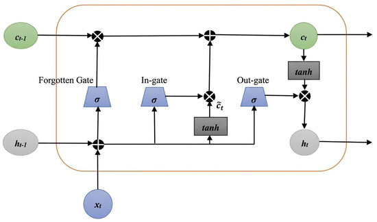
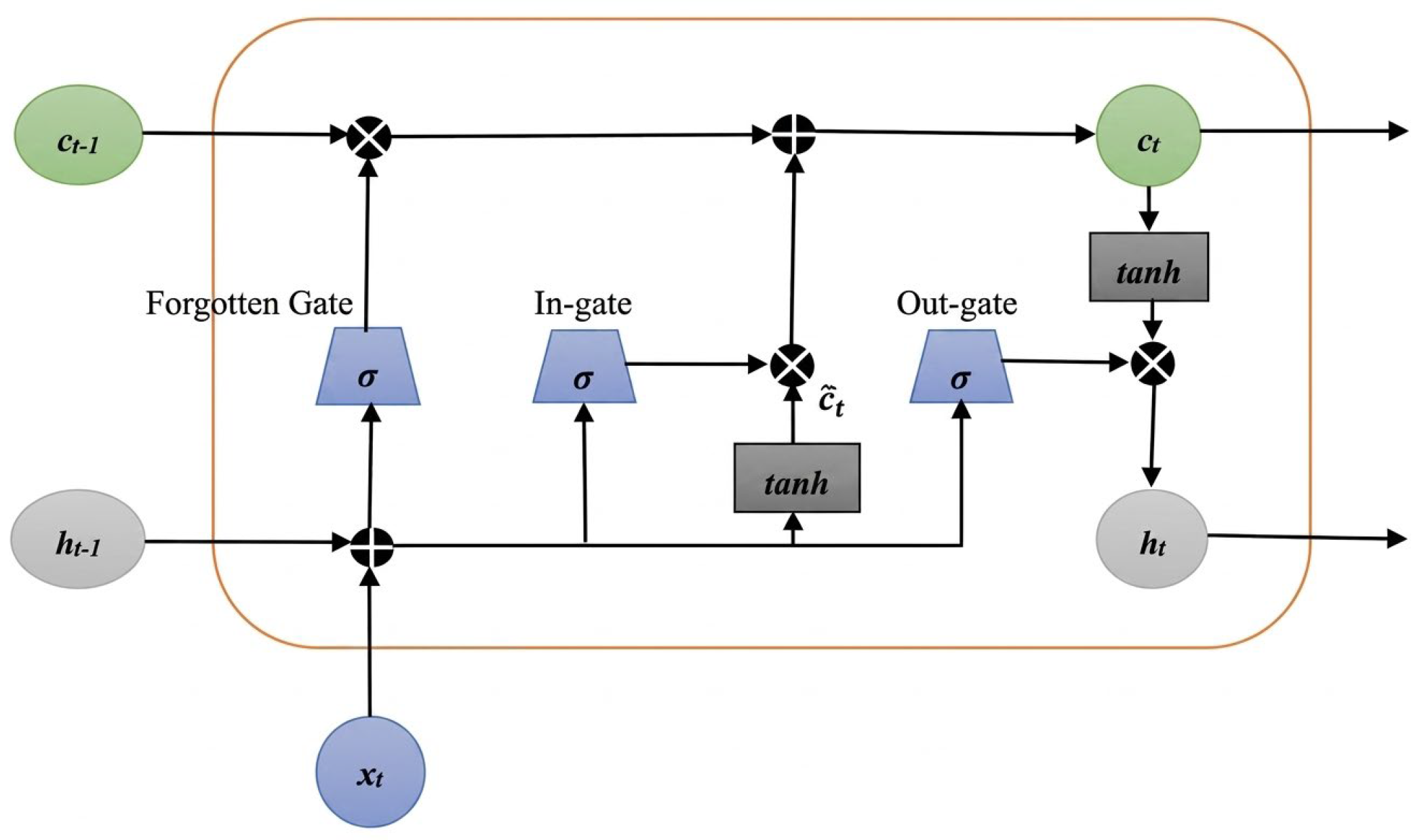
The LSTM can store and retrieve information adaptively according to input data characteristics, making it capable of classifying, processing, and predicting time series with complex temporal patterns, even when critical events are separated by large, variable, or unknown time intervals. Functionally, each LSTM block behaves as an intelligent network unit that can selectively “remember” or “forget” specific information over arbitrary time spans. Owing to its recursive connections among multiple nodes, training an LSTM layer is generally slower compared to standard RNN architectures. The structure of the LSTM unit is shown in Figure 1.
Figure 1.
LSTM neural network structure.
One of the key advantages of the LSTM is its ability to retain important data for extended periods without accumulating irrelevant information. This is achieved through the element-wise interactions of the logical and linear components in its memory cell, which are modulated by the input and output gates. These gates dynamically open or close depending on the logical state of the incoming data stream, allowing the network to admit or block information as required. Consequently, irrelevant data can be filtered out by closing the input gate, preserving long-term memory retention—a capability that standard RNNs inherently lack [10].
Unlike the standard recurrent unit that simply calculates the weighted sum of input signals, the input signals are then processed through a nonlinear activation function. Each j-th LSTM unit maintains a memory at time t. The output is the activation as shown below:
where is the output gate. The amount of memory content exposed is regulated according to:
Here, denotes a logical s-type function, and is a diagonal matrix. The memory unit is updated by partially erasing the existing data and adding new content .
The new memory content is:
The forgetting gate regulates the amount of information forgotten from the current memory. The input gate determines the quantity of new memory content added to the cell according to the following formula:
Here, and are diagonal matrices. As previously mentioned, standard recurrent neural networks fully cover all content at each time step. In contrast, LSTM units determine which memories to store through input/output gates. Thus, when an LSTM unit detects significant behavioral patterns in the input data, it applies corresponding weighting to the data and passes the information to the next time step [11]. This enables the network to capture potential long-term system dependencies.
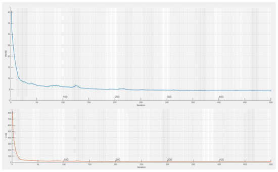
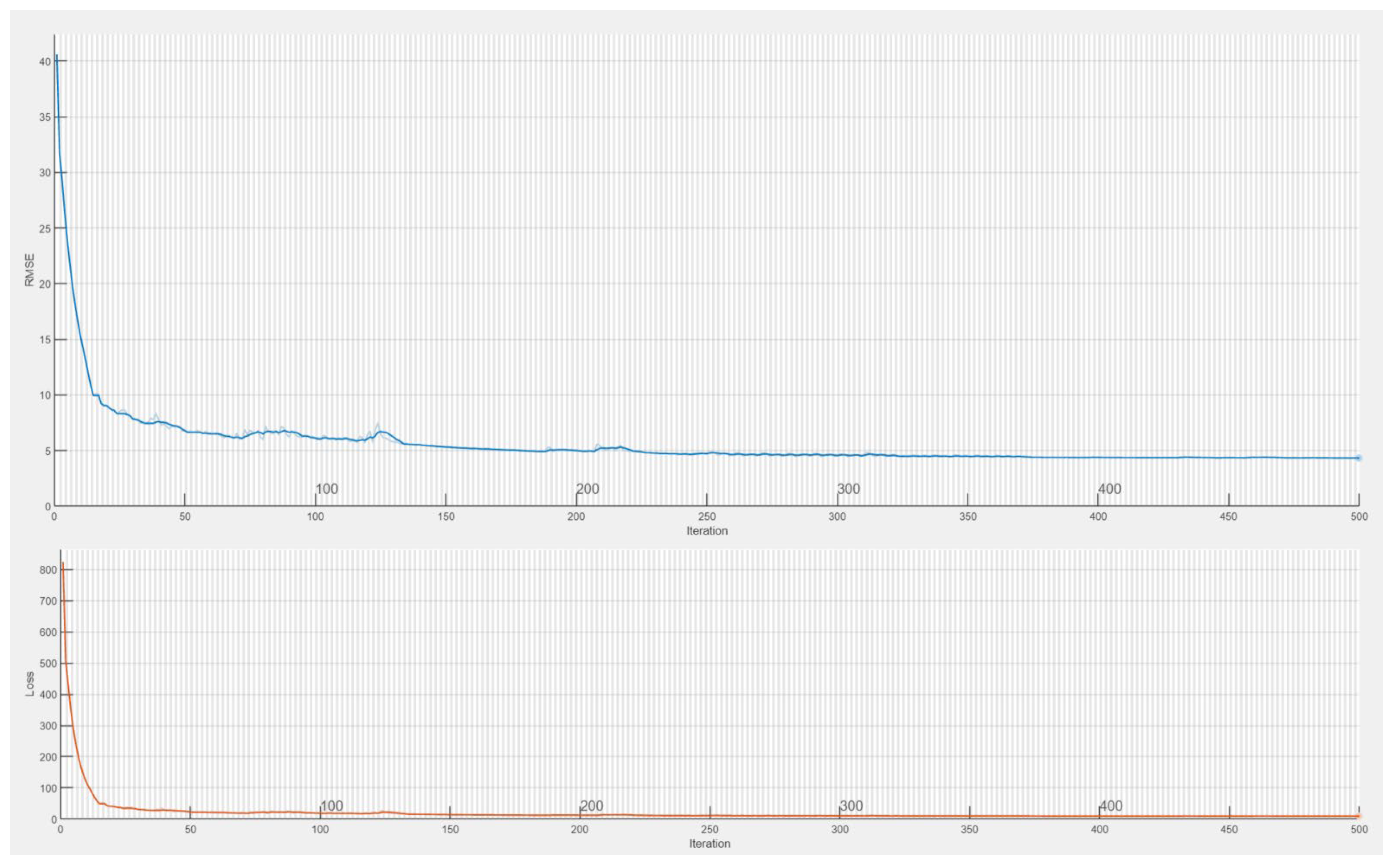
The training progress of the LSTM model is shown in Figure 2.
Figure 2.
LSTM training progress.
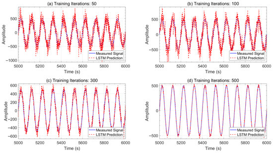
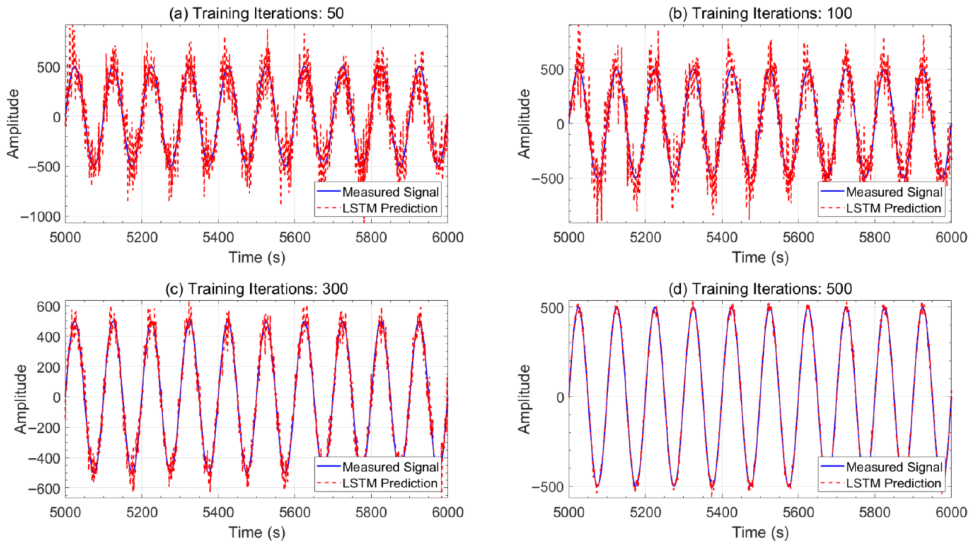
As the training progresses, the prediction performance will be further improved, as shown in Figure 3.
Figure 3.
LSTM prediction results improvement during training.
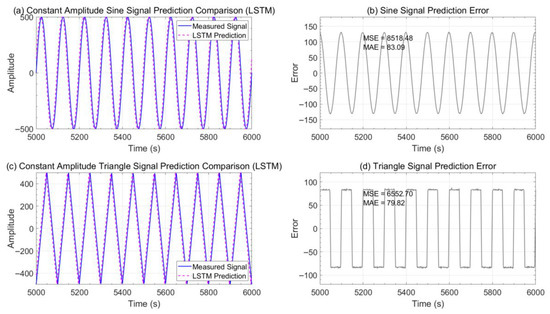
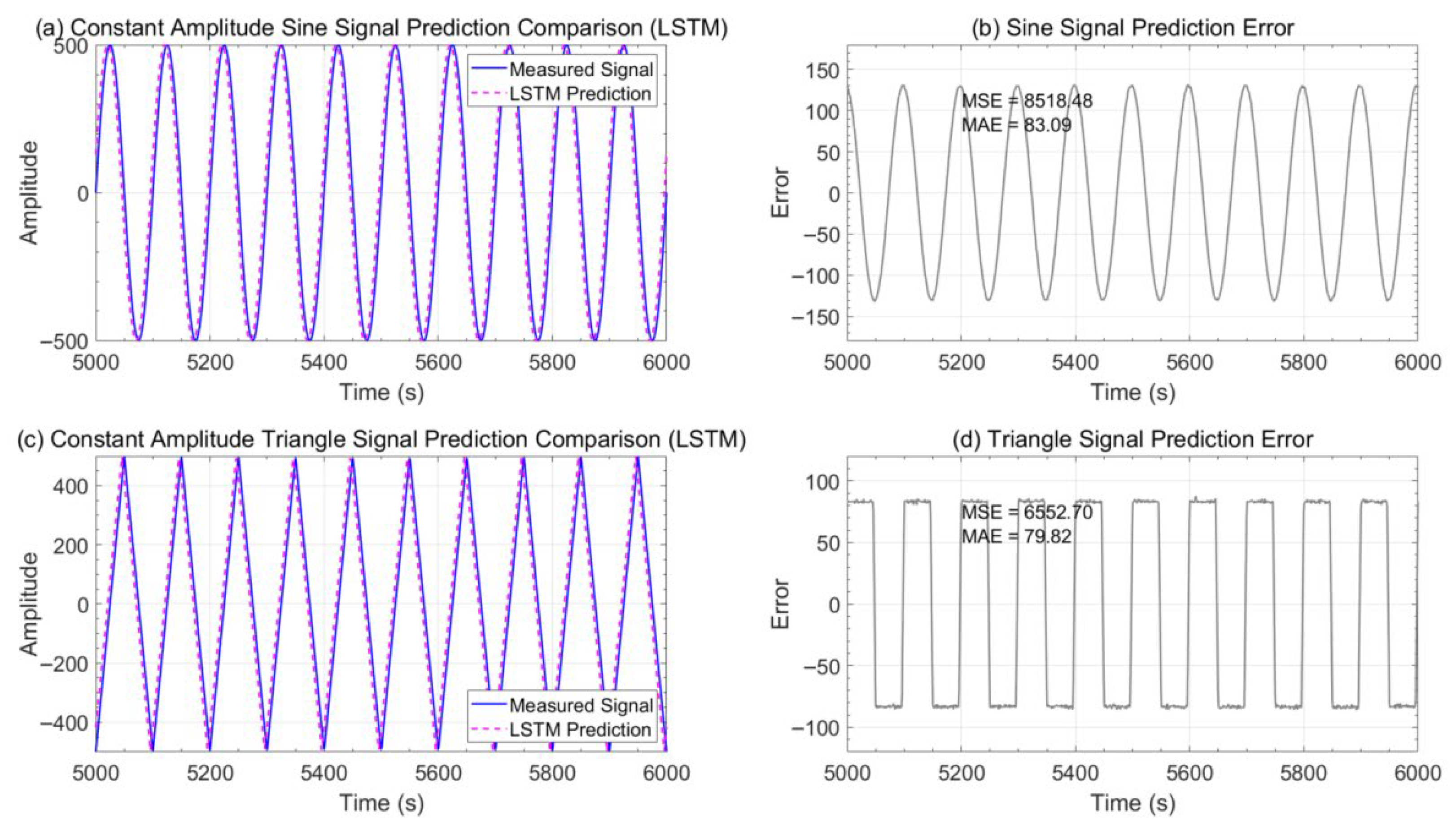
Figure 4 presents the LSTM model’s fitting results for both equal-amplitude sine and triangular signals. (a) compares the predicted power with the measured signal under the equal-amplitude sine signal, (b) displays the model’s hysteresis error under the same condition, (c) contrasts the predicted and measured signals under the equal-amplitude triangular signal, (d) shows the model’s hysteresis error under the triangular signal.
Figure 4.
LSTM prediction results for constant-amplitude signals.
As shown in Figure 4, the LSTM model demonstrates excellent fitting performance for equal-amplitude signals, with the model curve showing clear alignment with the actual curve.
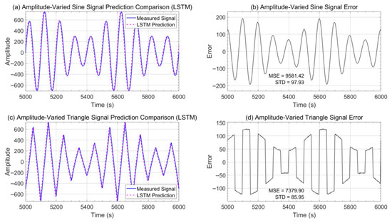
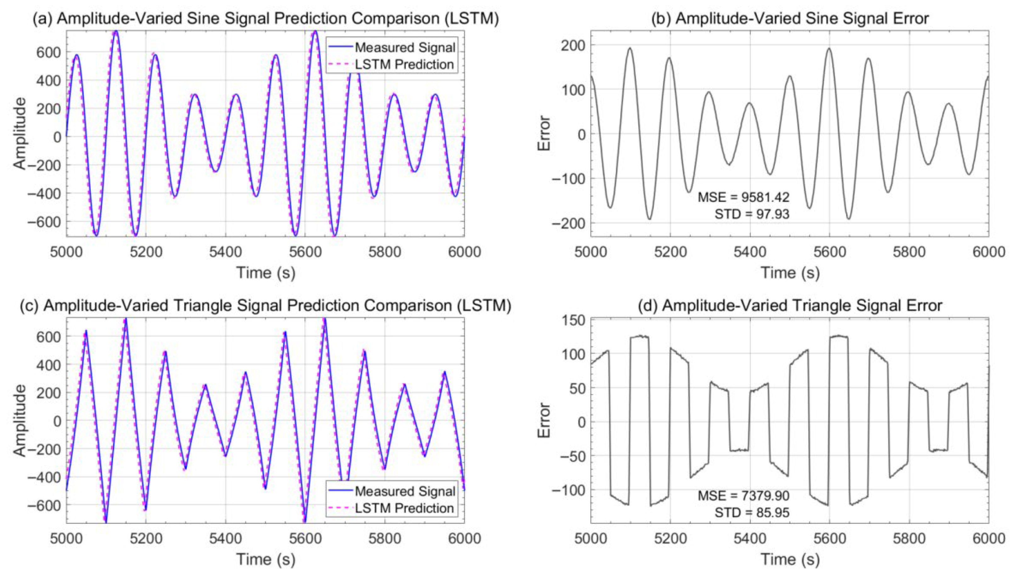
Figure 5 presents the LSTM model fitting results for amplitude-modulated sine and triangular signals. (a) compares the predicted power with the measured signal under constant-amplitude sine signal input, (b) displays the model’s hysteresis error under the same condition, (c) contrasts the predicted and measured signals under constant-amplitude triangular signal input, (d) shows the model’s hysteresis error under the same triangular signal input.
Figure 5.
LSTM prediction results for variable-amplitude signals.
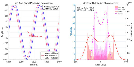
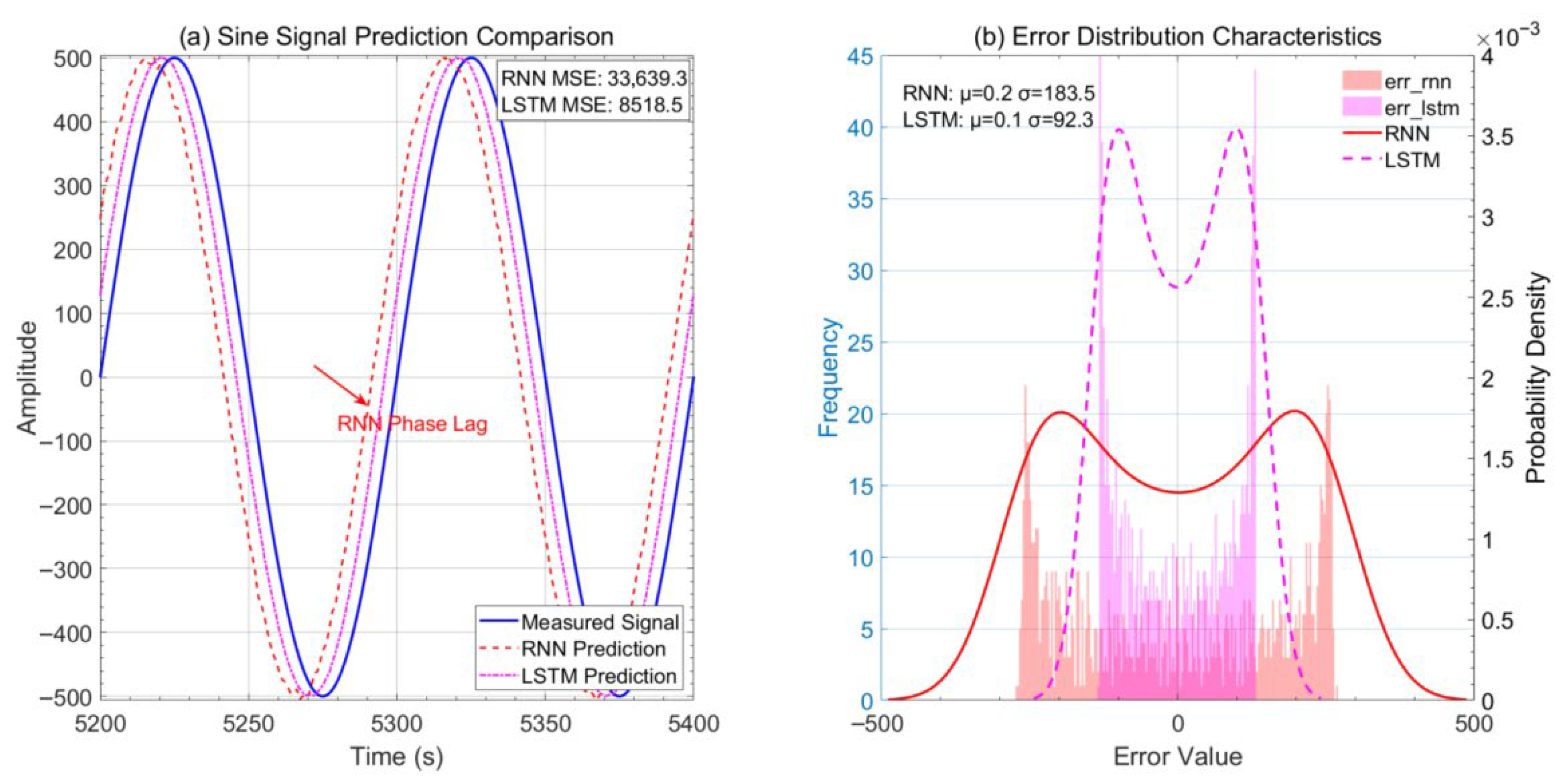
The comparison between LSTM and RNN models is shown in Figure 6. It can be seen that the LSTM model still has good fitting effect under the variable amplitude signal.
Figure 6.
Comparison of LSTM and RNN prediction performance.
A comparison between Figure 4 and Figure 5 clearly demonstrates that the LSTM model outperforms the RNN model in prediction accuracy. As the LSTM neural network requires a training process, its initial error is higher, with some maximum and minimum errors exceeding those of the RNN model. As shown in Figure 6, the LSTM model exhibits significantly better performance, with both its overall average error and root mean square error being substantially lower than those of the RNN model.
3. LSTM-LSSVM-CC Cascade Correction Prediction Model Design
3.1. Core Mechanism of the Method
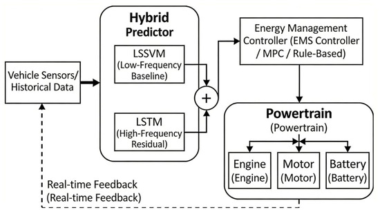
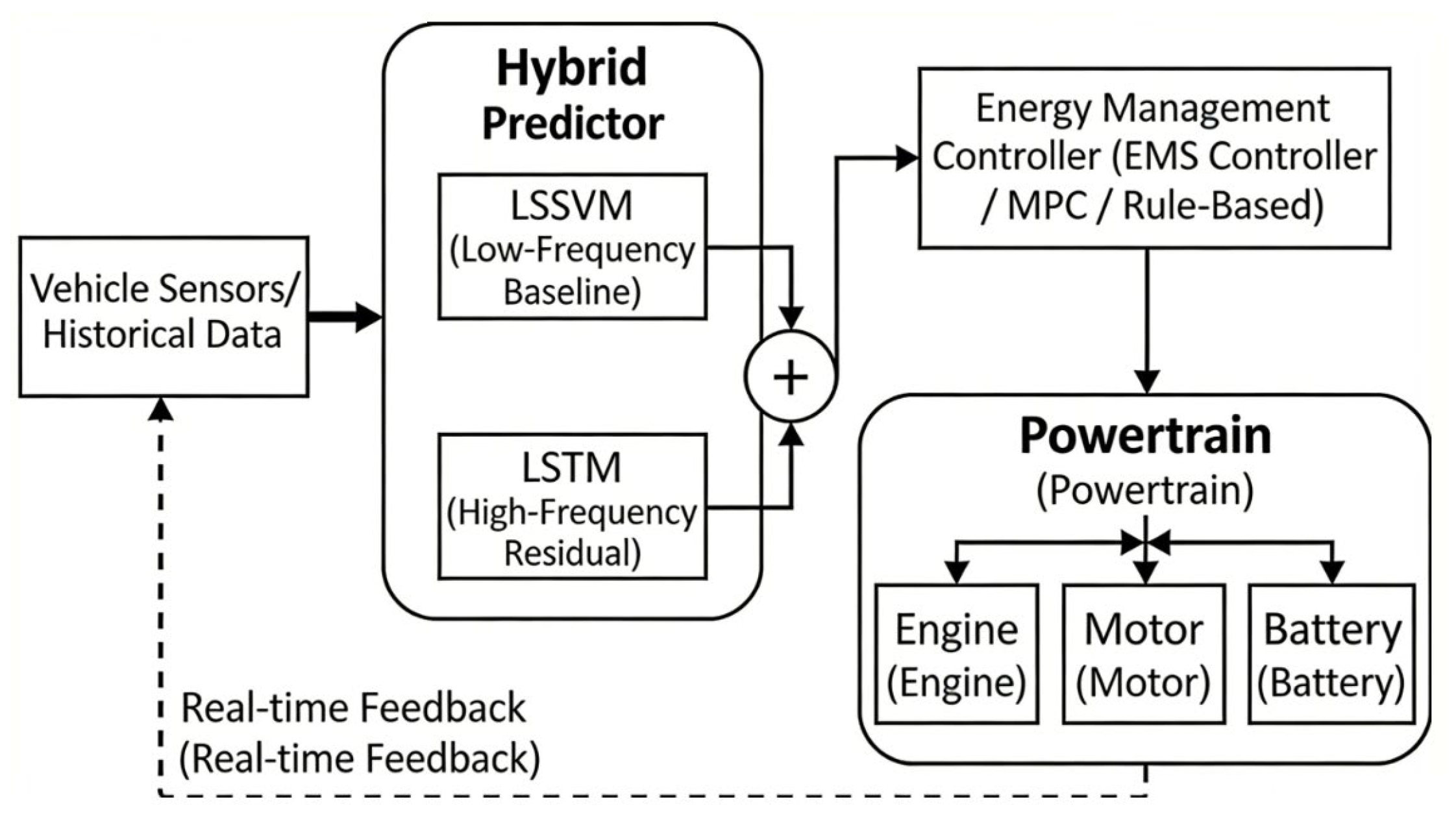
To clearly illustrate how the proposed data-driven predictor integrates with the hybrid electric vehicle (HEV) powertrain and the energy management controller, Figure 7 presents the overall system architecture [12,13,14,15,16,17,18,19]. As shown, the framework operates in a closed-loop manner: real-time sensor data feeds into the dual-stage prediction module (LSSVM for steady-state and LSTM for transients), generating a future power demand profile. This profile serves as the look-ahead input for the EMS controller, which subsequently optimizes the torque distribution between the engine and motor. This architectural view bridges the gap between the theoretical algorithm and its physical implementation.
Figure 7.
Overall architecture of the proposed LSTM-LSSVM-CC based energy management system for HEVs.
To address the insufficient capability of traditional models in characterizing dynamic behaviors in complex vehicle operating conditions, this paper proposes a hybrid prediction approach in which an LSTM network is employed to correct the predictions of an LSSVM model. The proposed method follows a two-stage modeling paradigm that combines the nonlinear fitting ability of the Least Squares Support Vector Machine (LSSVM) with the dynamic residual correction capability of the Long Short-Term Memory (LSTM) network, enabling high-precision prediction and optimization for complex driving conditions. The core mechanism and workflow of the proposed method are described in detail below.
The proposed model, termed the LSTM-LSSVM Cascade Correction (LSTM-LSSVM-CC), is based on a hybrid linear–nonlinear architecture. In this framework, the LSSVM is utilized to capture the fundamental components of the signal, while the LSTM dynamically learns the time-varying features of the residual sequence, thereby realizing progressive correction of prediction errors.
Optimization objective:
and are the parameter sets of the two-stage model, with the optimization process implemented in phases.
Step 1: In the original space modeling, LSSVM transforms the regression problem into a convex optimization problem with equality constraints:
Here, denotes the explicit mapping function, is the penalty factor, and represents the relaxation variable for prediction errors.
Step 2: Introduce Lagrange multipliers into the dual space analytical solution to construct the dual function:
The closed-form solution is derived by the KKT condition.
Here, is the kernel matrix, and under the linear kernel, is the kernel matrix, and under the linear kernel.
Forecasting function:
The model is least square optimal for stationary linear components, but sensitive to time-varying nonlinear residuals.
Step 3: Construct the depth dynamic residual sequence for the LSTM residual corrector: Let the main model predict the residual as , and construct the LSTM input–output pair: Input sequence: → Output: , where is the input sequence, and is the output sequence. The window size of 5 is determined based on the temporal characteristics of the vehicle power demand signal. Considering the trade-off between capturing short-term dynamic features and avoiding excessive computational complexity, a window size of 5 is sufficient to cover the immediate historical residual information required for correcting the LSSVM baseline errors, while preventing the model from overfitting to noise.
Mathematical implementation of the gating mechanism: The LSTM cell at each time step t contains the following differential equation system as shown in Table 1:
Table 1.
LSTM cell differential equations.
Minimize the mean square error using the Adam optimizer:
The 200-dimensional hidden layer gives the network the ability of multi-scale representation of non-stationary residuals.
Error propagation equation: The total error of cascade model is the coupling result of two-stage error:
The mean square error can be decomposed as:
When the LSTM satisfies the validity condition of residual prediction:
The cascade error is strictly smaller than the standalone prediction error of LSSVM.
This result suggests that LSTM can effectively reduce residual prediction errors by extracting predictable components from residuals, such as periodic fluctuations and trend drift.
3.2. Advantages and Workflow of the Method
The complementarity between linear and nonlinear models provides an efficient solution for analyzing complex signals. Among them, the Least Squares Support Vector Machine (LSSVM), based on the principle of structural risk minimization, possesses a rigorous theoretical framework and excels in handling low-frequency stationary components. By applying kernel-based feature mapping in the feature space, the LSSVM achieves unbiased estimation of stationary relationships [20,21,22,23].
In contrast, the Long Short-Term Memory (LSTM) network, with its unique forget gate and input gate mechanisms, is capable of dynamically adjusting the cell states and effectively capturing the complex dynamic characteristics contained in high-frequency non-stationary residuals [24].
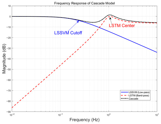
Through the cascade modeling framework, the combined LSSVM–LSTM model demonstrates a clear synergistic effect in the frequency domain: the LSSVM, serving as the base predictor, primarily responds to low-frequency components, while the LSTM residual corrector focuses on compensating and reconstructing high-frequency details. Together, their total response function forms complementary coverage across the entire frequency spectrum.
This dual-modal fusion strategy maintains the theoretical interpretability of the model while significantly enhancing the accuracy of non-stationary time-series modeling through nonlinear correction [25]. At the level of spectral energy distribution, the approach achieves an organic integration between global features and local fluctuations, thereby improving predictive precision across all dynamic operating conditions. The total response function of the cascade model is expressed as:
It covers all frequency band signal components (as shown in Figure 8).
Figure 8.
Frequency response of the cascade model.
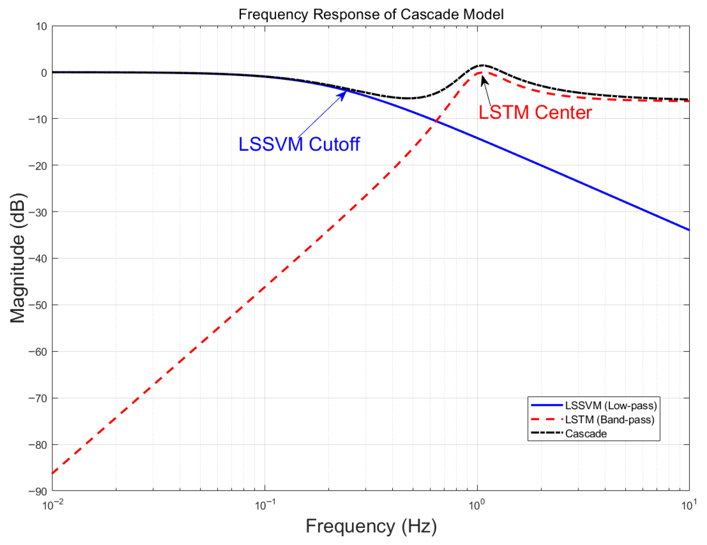
As quantitatively shown in Figure 8, the cascade model achieves full-spectrum coverage through explicit frequency-domain division of labor. The LSSVM module (blue solid line) behaves as a low-pass filter with a cutoff frequency at approximately 0.5 Hz, effectively suppressing high-frequency noise while preserving the dominant low-frequency trend of the driving cycle. In contrast, the LSTM module (red dashed line) functions as a band-pass/high-pass compensator, peaking around 1.0 Hz to capture rapid transients and local fluctuations that LSSVM misses. Crucially, their superposition (black dotted line, “Cascade”) yields a nearly flat magnitude response across the entire operational bandwidth (0.01–10 Hz), confirming that the two components are spectrally complementary—neither overlapping nor leaving gaps. This engineered spectral partitioning is the fundamental reason why the hybrid model outperforms single architectures under dynamic conditions.
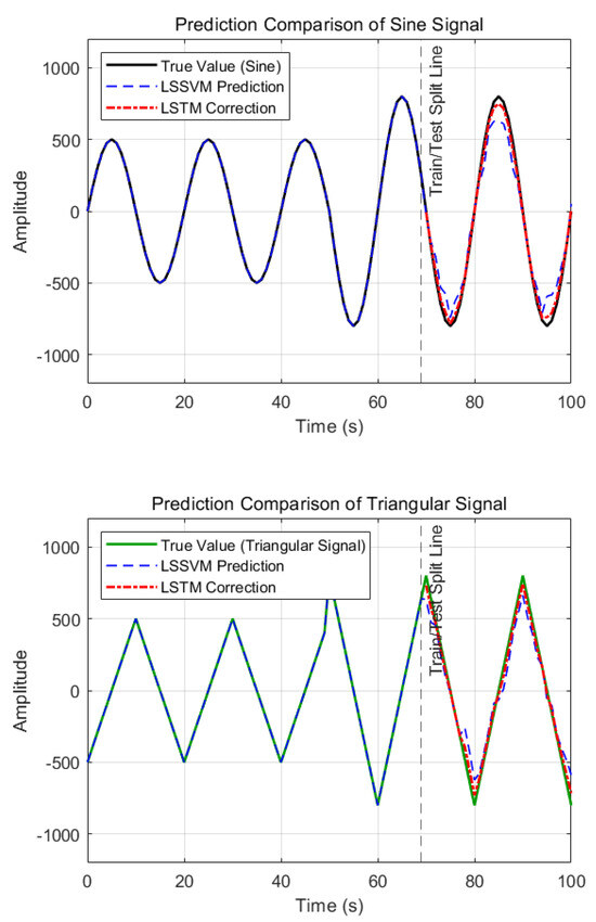
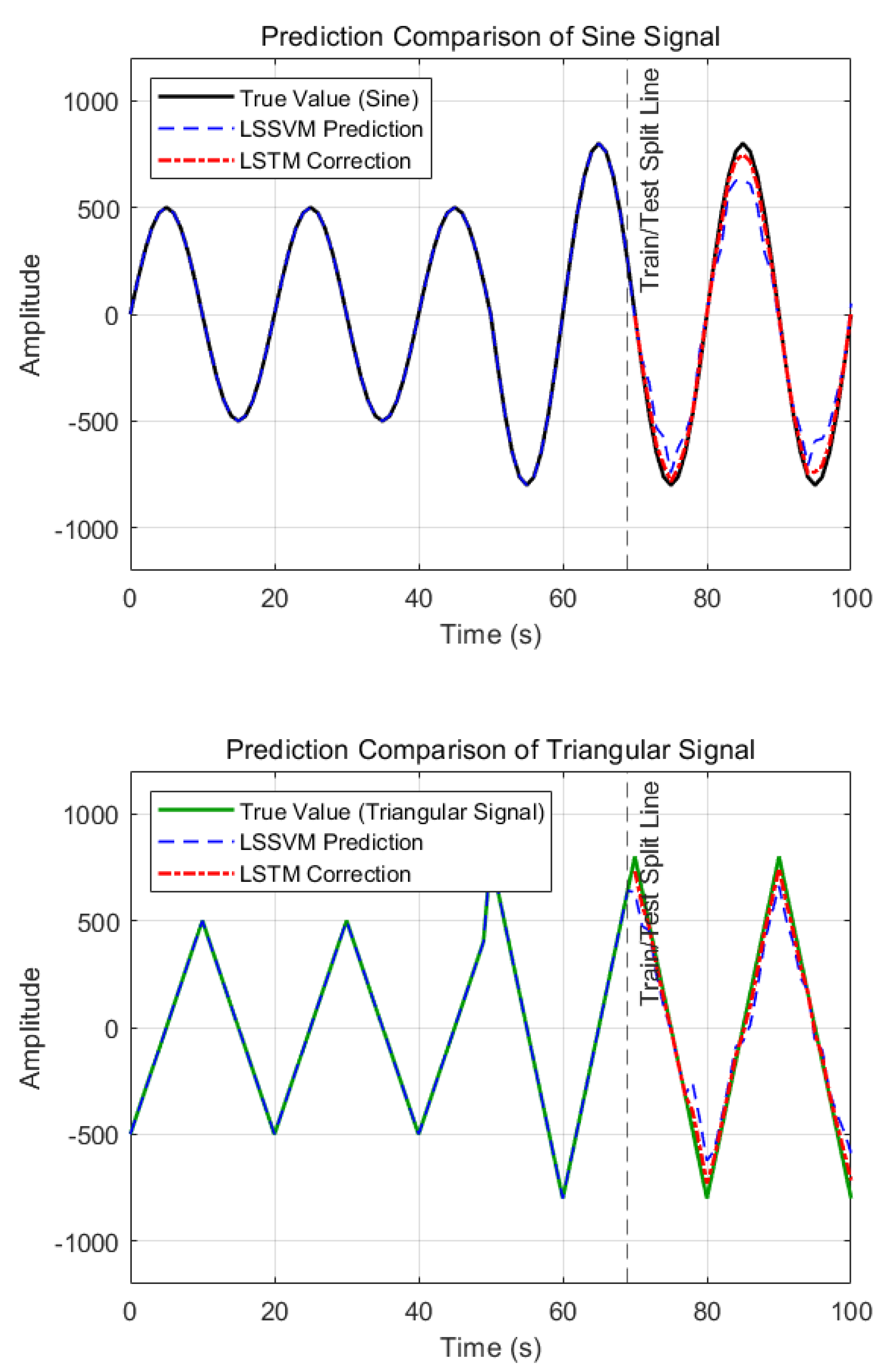
In time-varying adaptive modeling of dynamic systems, Long Short-Term Memory (LSTM) networks demonstrate exceptional responsiveness to abrupt load amplitude changes through their gating mechanisms. The unique architecture of LSTM features a dynamic gradient adjustment system formed by the forgetting gate and input gate. When detecting abrupt features in external input signals , the forgetting gate dynamically adjusts memory retention ratios based on the current cell state and input Meanwhile, the input gate updates the cell state by filtering relevant information through the sigmoid function. This regulatory process is mathematically represented as a cross-time-step gradient propagation chain rule:
The model demonstrates how LSTM decouples long-range dependencies through the product form of accumulated partial derivatives, enabling rapid weight parameter correction under sudden load changes. This time-varying adaptation mechanism effectively suppresses nonlinear disturbances caused by abrupt changes. By dynamically adjusting information storage cycles and update intensities, it maintains stable historical state transmission while enhancing the model’s ability to track unexpected events, significantly improving the robustness of dynamic system parameter identification. The results are illustrated in Figure 9.
Figure 9.
Prediction comparison.
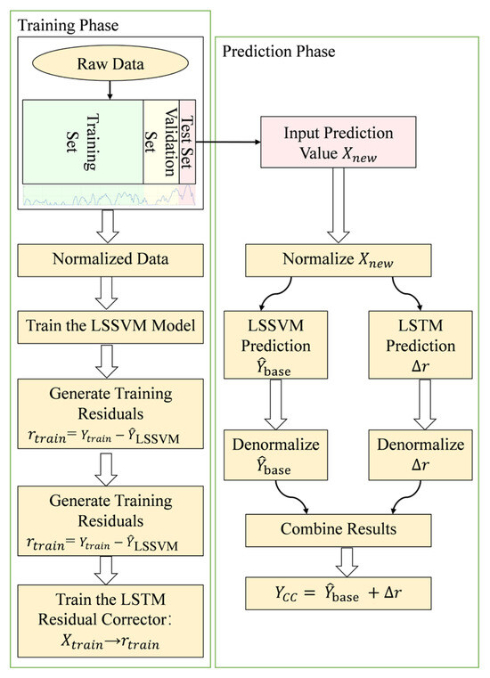
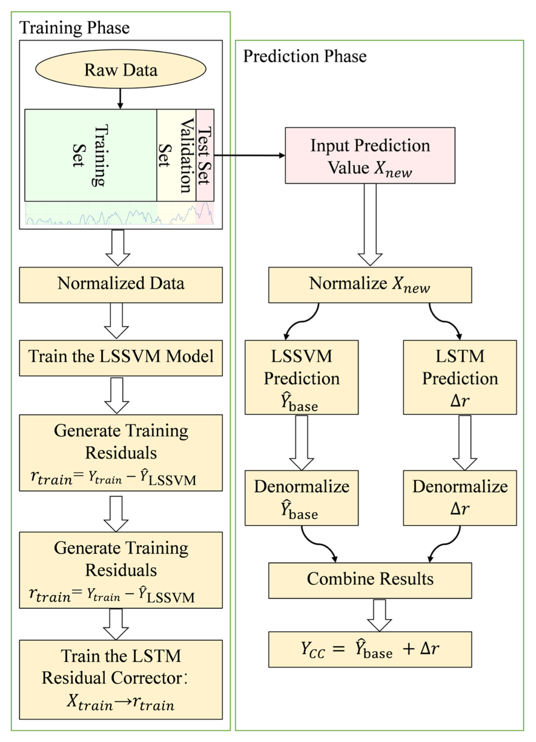
The proposed methodology consists of two distinct phases, Training and Prediction, as illustrated in Figure 10. During the training phase, raw time-series data are first standardized using a 7:2:1 split for training, validation, and testing sets, respectively. A Linear Support Vector Machine (LSSVM) base model is then trained on the normalized dataset by solving a regularized least-squares optimization problem to obtain optimal kernel parameters. Subsequently, residual sequences—defined as the difference between actual values and LSSVM predictions—are computed from the training set. These residuals serve as targets for training a 200-cell Long Short-Term Memory (LSTM) network, which takes the normalized training data as input. The LSTM is optimized via the Adam optimizer over 10 epochs to learn high-frequency error patterns.
Figure 10.
Workflow of the LSTM-LSSVM-CC method.
In the prediction phase, newly incoming data undergo identical standardization before being fed simultaneously into both the LSSVM and LSTM models. The LSSVM generates fundamental frequency-level forecasts, while the LSTM produces high-frequency residual corrections. Both outputs are subsequently back-standardized and algebraically summed to yield the final fused prediction. This cascaded architecture—combining a linear model with a nonlinear neural network—enables progressive, hierarchical error correction. Crucially, during training, test data are strictly isolated to prevent information leakage. In prediction, consistency in data scale is preserved through the standardization–back-standardization pipeline, thereby establishing a closed-loop error correction mechanism along the residual transfer path.
4. Simulation Design and Multi-Condition Prediction Performance Verification
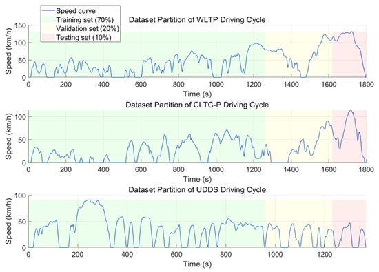
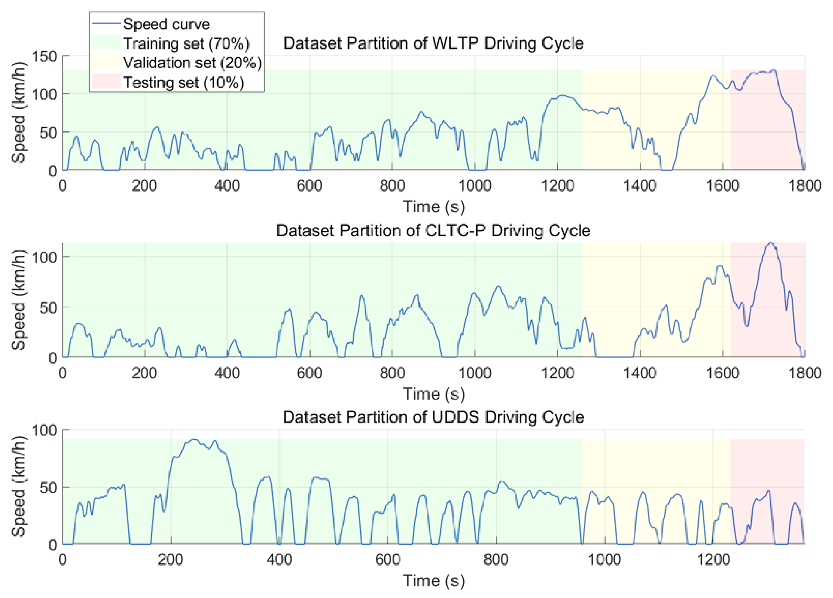
This section describes the construction of the prediction datasets in detail based on three standard driving cycles—CLTC-P, WLTP, and UDDS—as well as the setup of the simulation platform, which together provide the data and technical foundation for subsequent condition prediction experiments [26]. The data from the three driving conditions are divided into training, validation, and testing sets in a ratio of 7:2:1, ensuring uniform distribution of each driving condition across the training and testing stages. This partitioning effectively prevents the model from overfitting to specific driving patterns. The results are illustrated in Figure 11.
Figure 11.
Dataset division for three driving cycles.
In this study, multi-step prediction experiments were conducted under three typical driving conditions—CLTC-P, WLTP, and UDDS—by varying the prediction horizons (1, 3, and 5 s) and the dynamic characteristics of the driving conditions to construct multi-level validation scenarios. The models included in the comparison are LSSVM, Random Forest (RF), basic RNN, ELMAN network, independent LSTM, and the LSSVM–LSTM hybrid model. The experimental system was implemented on the MATLAB R2023b/Simulink platform using multi-threaded parallel computation. The key experimental parameter settings are shown in Table 2.
Table 2.
Experimental parameters for prediction models.
Note on Parameter Optimization: The core parameters listed in Table 2 were not arbitrarily selected but determined through a grid search strategy combined with 5-fold cross-validation on the validation set. The optimal values were chosen to minimize the Root Mean Square Error (RMSE) while balancing model complexity and generalization capability. For instance, 200 LSTM cells represented the trade-off point between underfitting (<100) and overfitting (>300), while a Dropout rate of 0.2 provided the best regularization effect. Crucially, the test set remained completely unseen during this tuning process to ensure an unbiased evaluation.
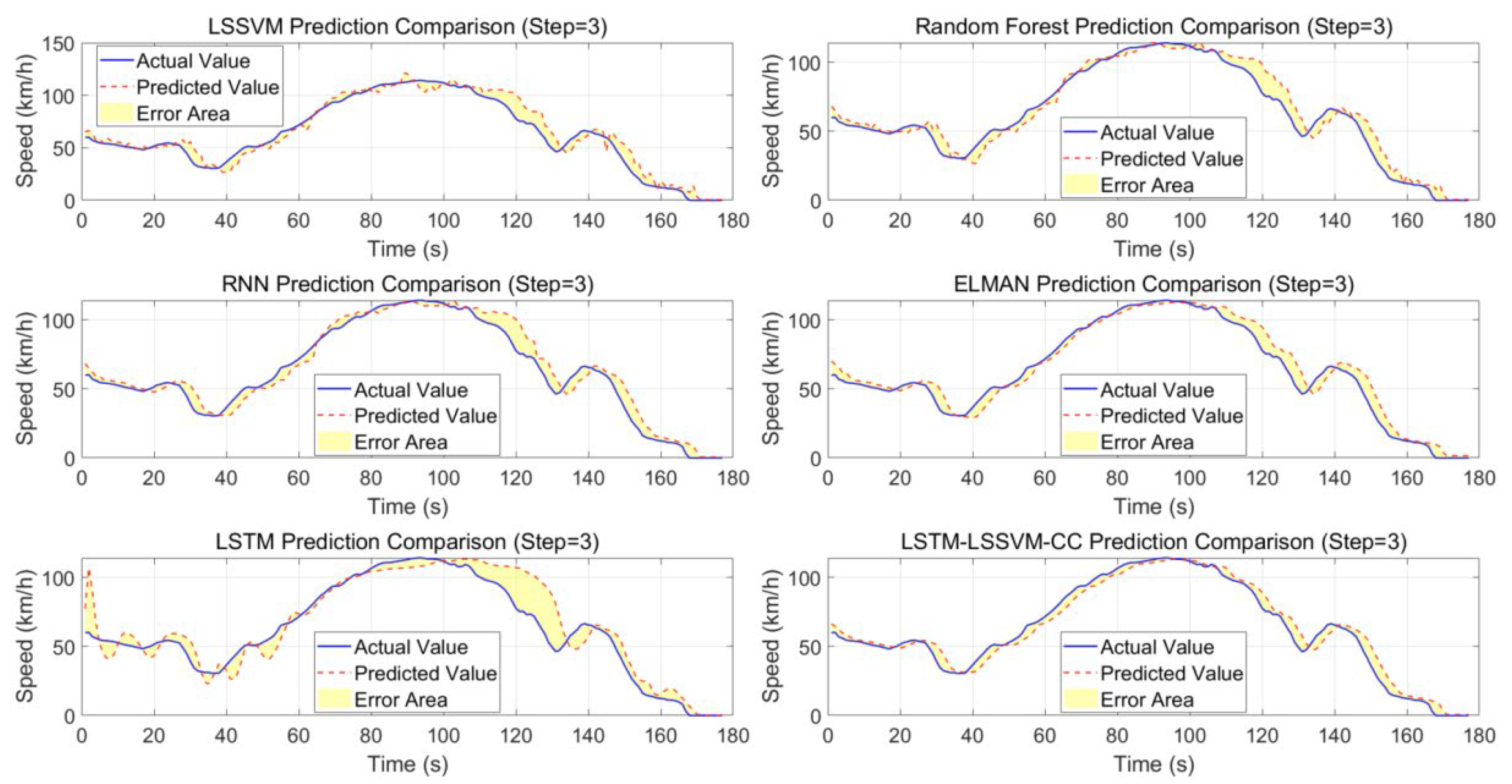
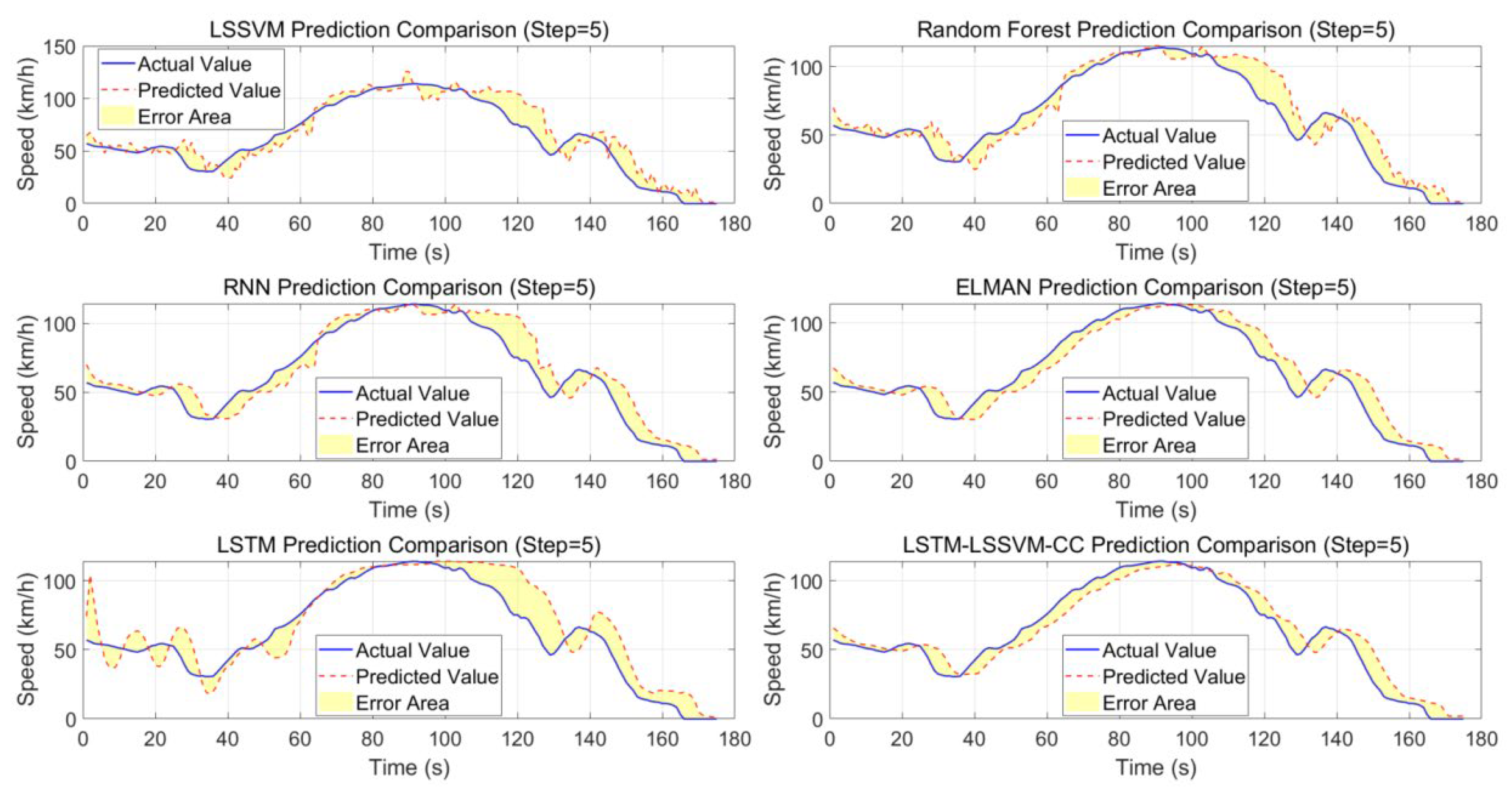
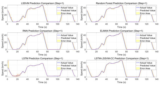
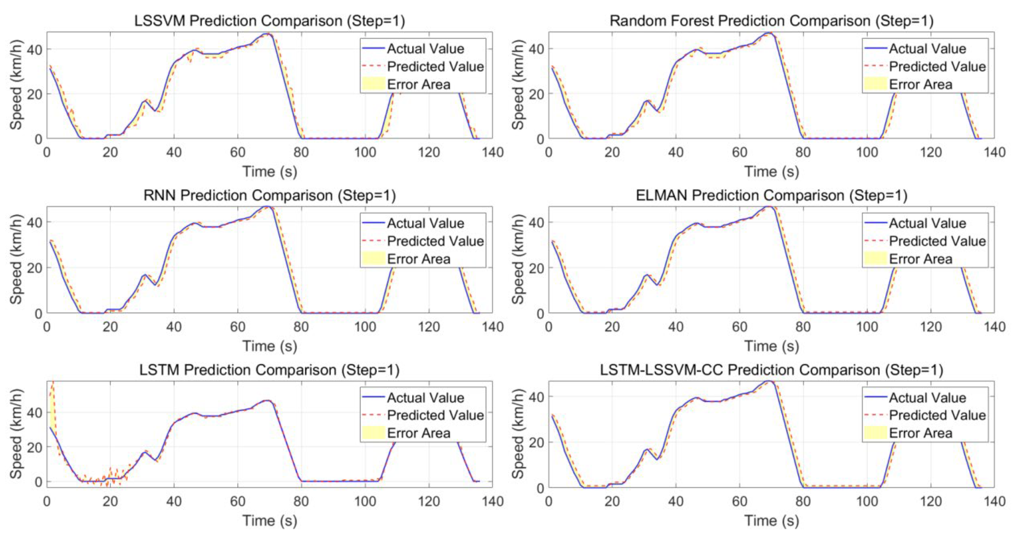
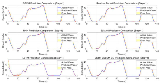
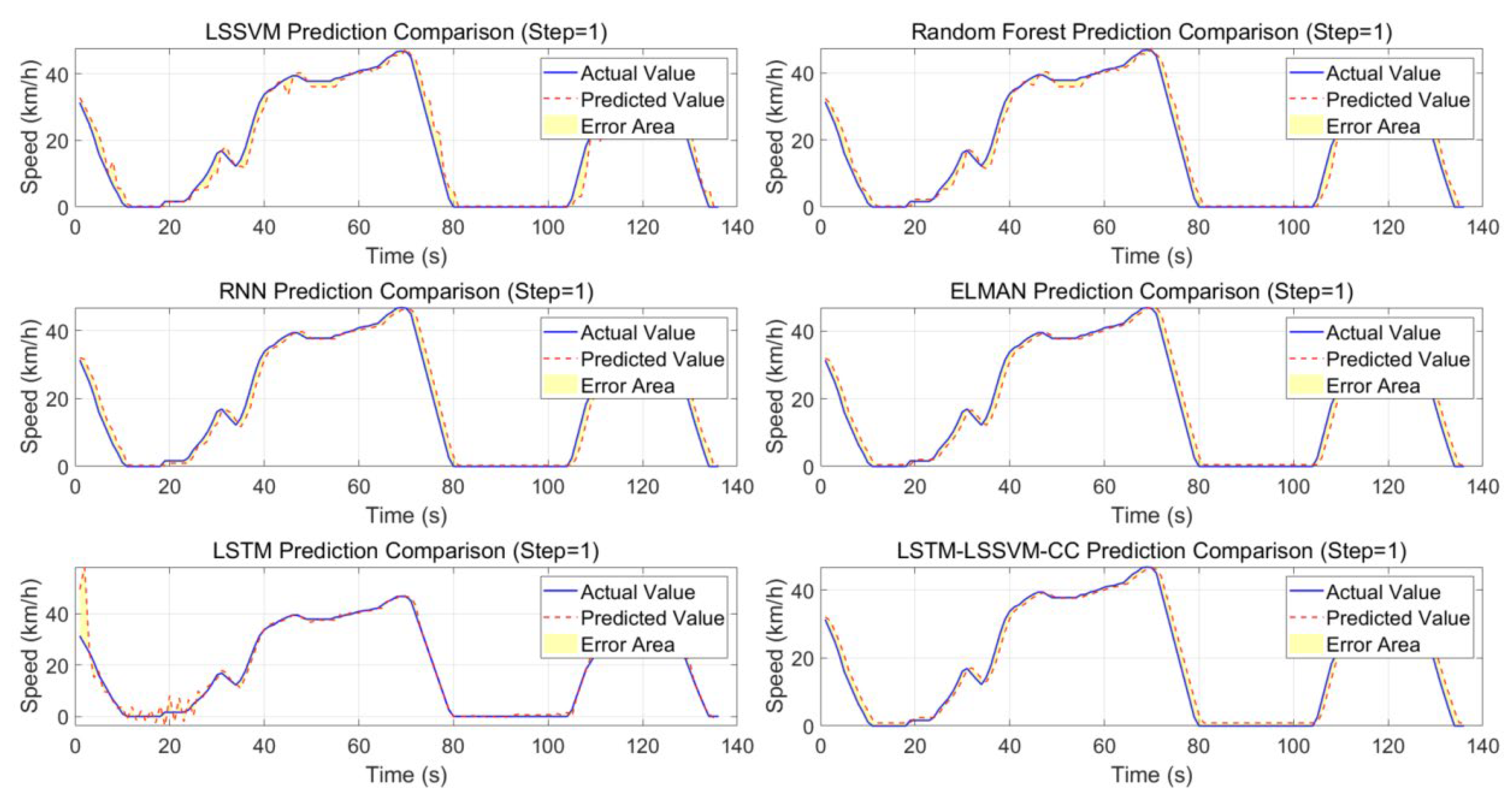
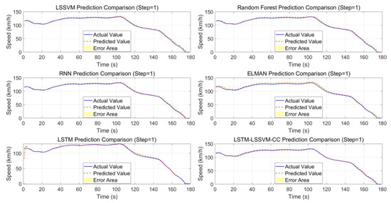
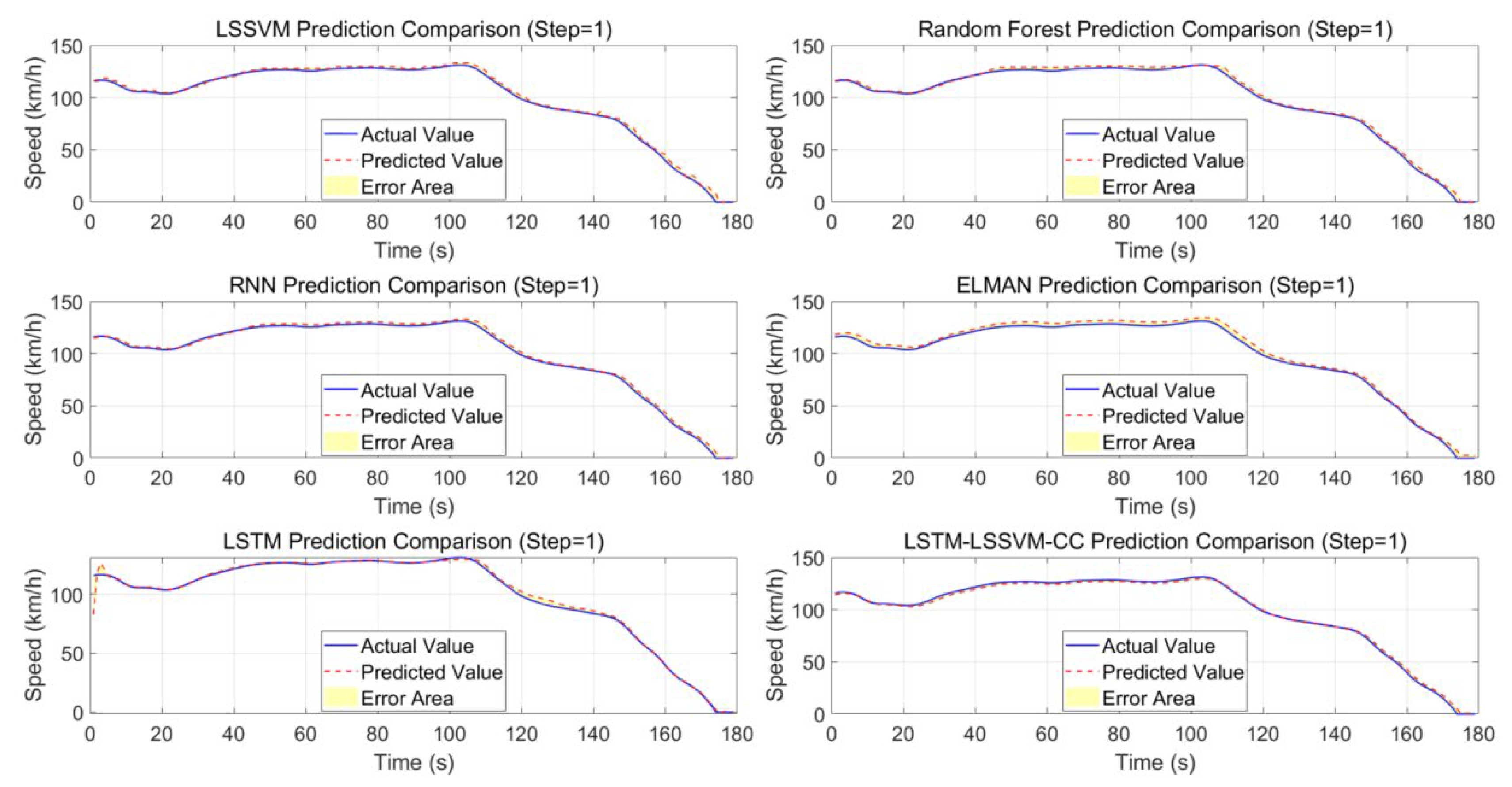
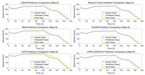
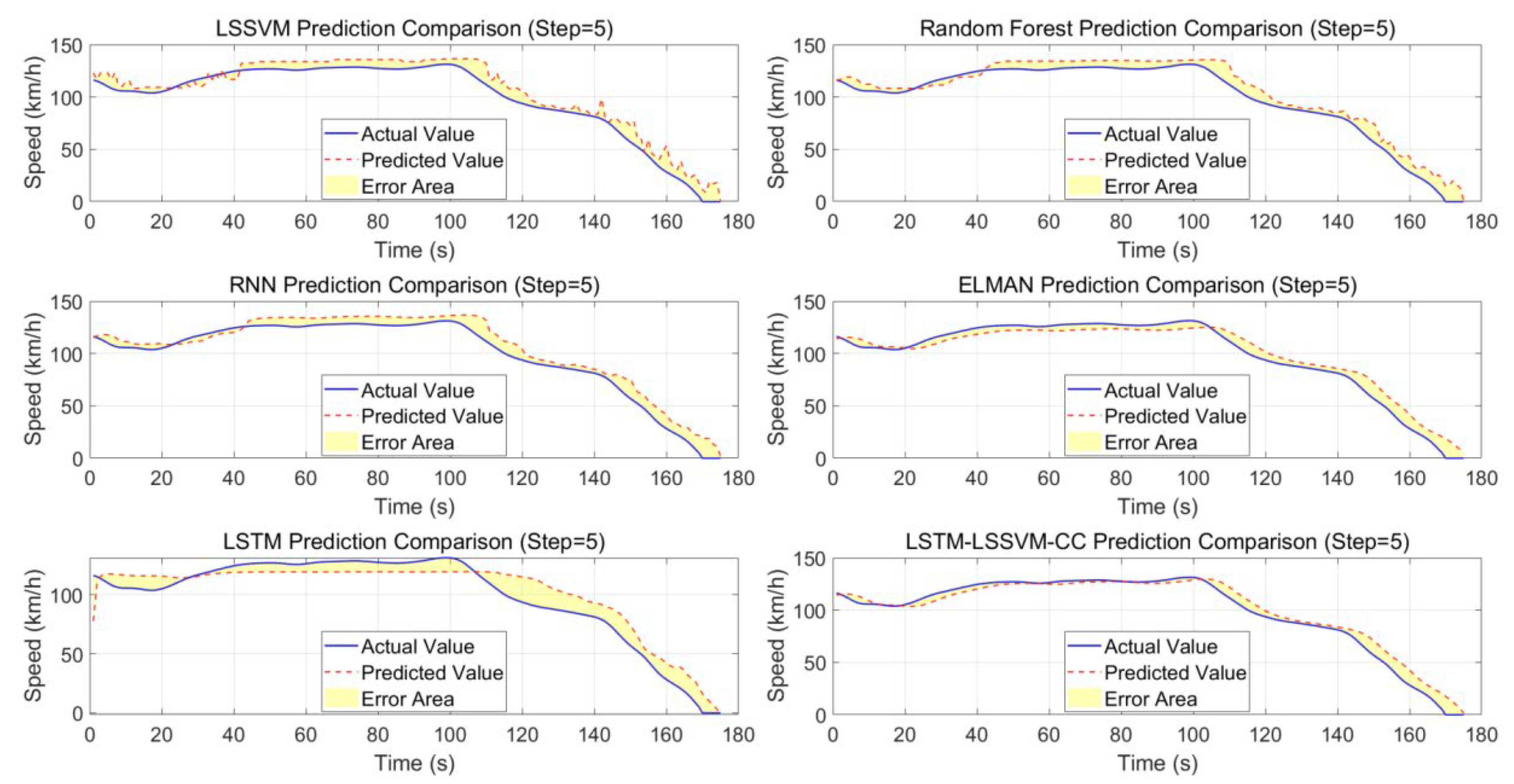
The comparison of prediction performance in Figure 12, Figure 13 and Figure 14 demonstrates that the LSTM-LSSVM hybrid model achieves significantly better trajectory matching than other models within the 1–5 s time step range. In the CLTC-P scenario with low average vehicle speed (29.0 km/h) and high idle duration (22–25%), the hybrid model effectively mitigates error accumulation through its dynamic residual compensation mechanism.
Figure 12.
CLTC-P 1 s prediction results comparison.
Figure 13.
CLTC-P 3 s prediction results comparison.
Figure 14.
CLTC-P 5 s prediction results comparison.
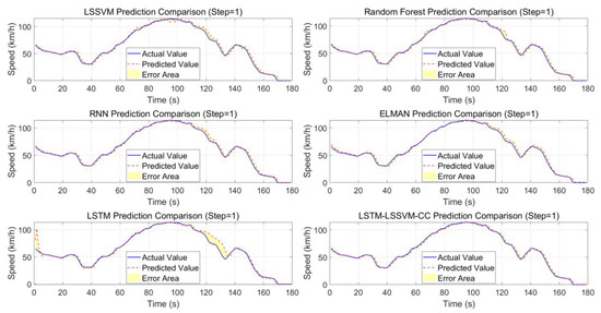
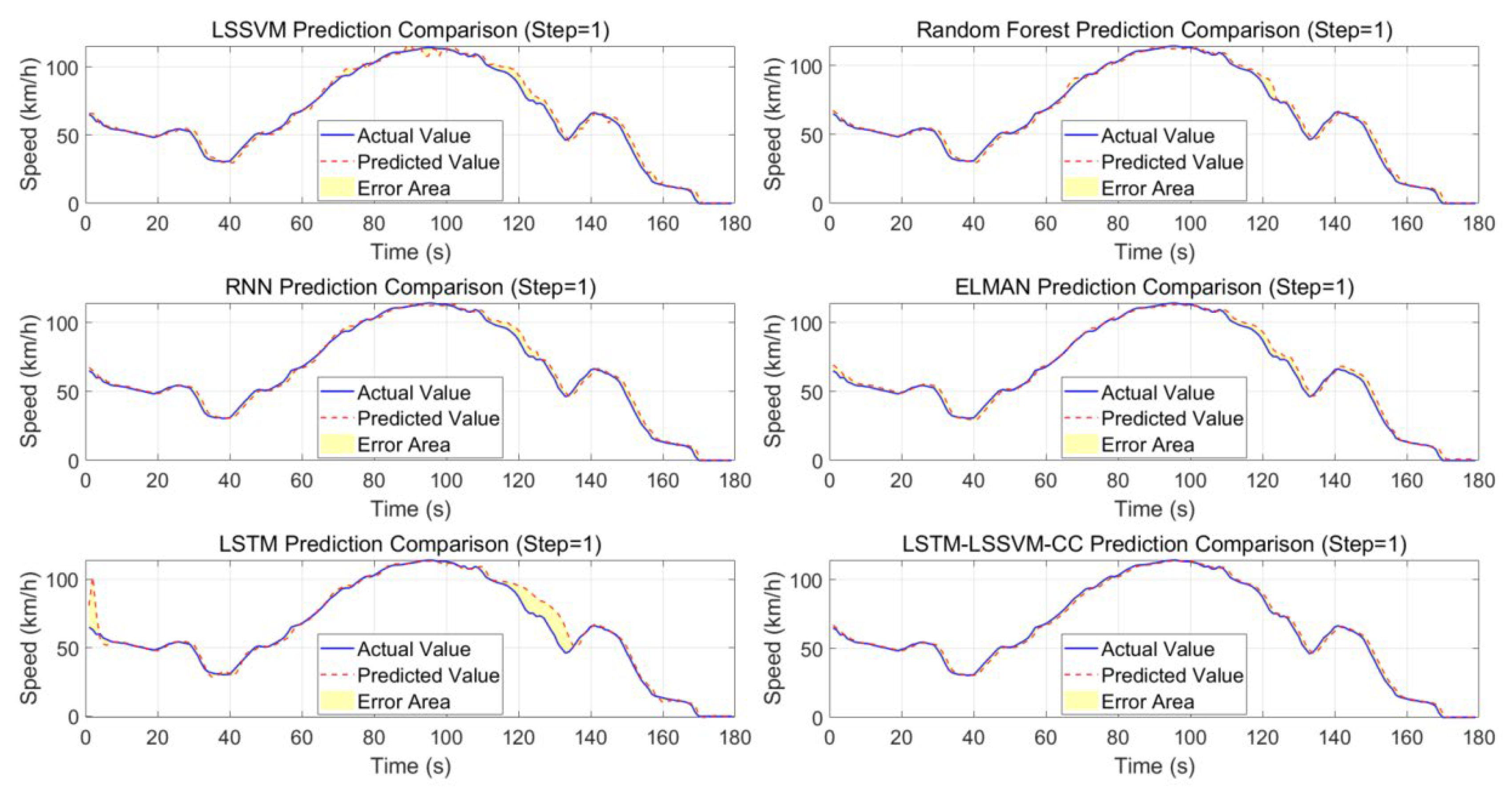
In the 1 s prediction results (Figure 14), the LSTM model’s predictions closely match actual values, though significant deviations occur at specific time points. For instance, the 2 s prediction value of 102.309 shows a notable discrepancy with the actual value of 63.4. The LSTM-LSSVM-CC model demonstrates overall stability, with predictions consistently aligning with actual values across most time points. During the 1–10 s interval, predicted values fluctuate within a narrow range of actual values. Other models (LSSVM, Random Forest, RNN, and ELMAN) exhibit varying performance: LSSVM’s 1 s prediction of 65.789 closely matches the actual value of 65.1, but shows substantial deviations from actual values after 170 s. The LSTM-LSSVM-CC model maintains stable predictions with minimal fluctuations and close alignment to actual values, indicating its superior stability.
As shown in Figure 13, the LSTM model’s predictions generally align well with actual values across most time points, though a notable deviation occurs at the 2 s mark (predicted value: 102.629 vs. actual value: 60.2). In contrast, the LSTM-LSSVM-CC model demonstrates superior stability, maintaining consistent predictions with minimal fluctuations. Specifically, during the 1–10 s interval, its predicted values fluctuate within a narrow range around the actual values.
As shown in Figure 14, the LSTM-LSSVM-CC model demonstrates a superior performance across most time points, exhibiting stable predictions with minimal fluctuations and close alignment to actual values. In contrast, models like RNN and ELMAN show significant fluctuations at certain time points, indicating relatively poorer stability. Overall, the LSTM-LSSVM-CC model excels in prediction accuracy, trend capture capability, and stability, making it particularly suitable for short-term forecasting and capable of accurately identifying data trends. To further validate the model’s comprehensive performance in predicting power demand for hybrid vehicles, this section compares two typical test datasets—UDDS (Urban Road Cycle) and WLTP (Worldwide Harmonized Light Vehicle Test Cycle)—under 1 s and 5 s prediction step lengths, respectively. The results are presented in Figure 15, Figure 16, Figure 17 and Figure 18.
Figure 15.
UDDS 1 s prediction results comparison.
Figure 16.
UDDS 5 s prediction results comparison.
Figure 17.
WLTP 1 s prediction results comparison.
Figure 18.
WLTP 5 s prediction results comparison.
Under the UDDS test conditions, during the abrupt change period (4–10 s), the actual power dropped sharply from 20.92 to zero. The LSTM model showed a 26% deviation (−26%,15.5 vs. 20.9) in its prediction at the 4 s mark, while the LSTM-LSSVM-CC model maintained a 16% deviation (+16%,24.3 vs. 20.9). In the zero-value interval (points 11–18), the LSTM exhibited abnormal oscillations (e.g., point 15: −0.9 vs. 0), whereas the LSTM-LSSVM-CC remained stable at 0.73, approaching the actual zero value. For the high-power interval (35–45 s), the actual power ranged from 37.8 to 39.4, with the LSTM’s prediction fluctuating wildly (35.5–38.9, SD 8.2). In contrast, the LSTM-LSSVM-CC model showed smoother fluctuations (37.6–38.9, SD 0.7).
For WLTP conditions, peak tracking (42–45 s) showed actual power between 123.8–125.4, with LSTM predictions at 122.8–124.1 (averaging 1.2% lower) and LSTM-LSSVM-CC at 121.1–123.1 (averaging 1.8% lower), while LSSVM exhibited significant overestimation (124.3–127.8, 3.5% higher). During low-power decay (155–160 s), actual power dropped from 54.6 to 39.9, with LSTM predictions plummeting from 51.9 to 36.7 (±15% error fluctuation), whereas LSTM-LSSVM-CC smoothly decreased from 56.4 to 42.9 (±5% error fluctuation).
Under high-frequency fluctuations in the UDDS test conditions (e.g., during 20–24 s), the actual value surged from 1.6 to 2.57, while the LSTM prediction dropped from 6.2 to 5.2 (reverse fluctuation). The LSTM-LSSVM-CC model showed a synchronous increase from 2.3 to 2.5. During 55–60 s, the actual value stabilized at 40.8–41.3, with the LSTM prediction rising from 38.7 to 40.2 (lagged increase). The LSTM-LSSVM-CC model exhibited no lag, rising synchronously from 38.5 to 40.1.
5. Model Performance Comparison and Advantage Analysis
This experiment validates the superiority of the proposed hybrid model by comparing the multi-step prediction performance of LSTM-LSSVM-CC, LSSVM, Random Forest, RNN, ELMAN, and standalone LSTM models under three operational conditions: CLTC-P, UDDS, and WLTP. The results demonstrate that LSTM-LSSVM-CC exhibits significant error suppression capability and dynamic adaptability across all test scenarios. In short-term predictions (1 s), its RMSE is reduced by approximately 28–36% compared to suboptimal models (e.g., 1.753 vs. 2.493 for LSSVM in CLTC-P), with MAE narrowing to 0.06 percentile error and TIC coefficient below 0.015, indicating high synchronization between predicted curves and real values. Particularly in high-dynamic conditions (e.g., WLTP peak power fluctuations and UDDS frequent start-stop cycles), the hybrid model achieves rapid mutation signal tracking through LSTM gating mechanisms, reducing maximum error by 48% compared to LSSVM (20.30 vs. 37.42 in WLTP-5s). The error accumulation rate (slope of incremental growth per second) is only 0.13%/s, significantly lower than the LSTM’s 0.41%/s. In the long-term prediction (5 s) scenario, the LSTM-LSSVM-CC model achieved an error standard deviation of 6.19 (CLTC-P) to 8.42 (UDDS), representing a 52% reduction compared to conventional models. Its R2 coefficient remained stable within the 0.87–0.99 range, demonstrating effective global feature learning for non-stationary time series.
The performance analysis demonstrates that in the idle-dominated CLTC-P scenario, the hybrid model compensates for the LSSVM’s lag in zero-value zone response through a residual corrector (error mean reduced from −0.18 to −0.06). In the transient-frequent UDDS test, its TIC coefficient (0.166) is 31.7% lower than the Random Forest model’s (0.243), indicating significant improvement in trajectory similarity optimization. During high-dynamic WLTP testing, the hybrid model excels in correcting asymmetric error distribution (negative skewness −0.73), reducing the 75th percentile error by 42.1% compared to standalone LSTM. Furthermore, the hybrid model achieves computational efficiency of 0.083 s per sample in 5 s predictions, meeting real-time requirements. Parameter sensitivity analysis shows its robustness to kernel function bandwidth (σ) is approximately 23% higher than traditional LSSVM. In summary, the LSTM-LSSVM-CC model integrates LSSVM’s global optimality with LSTM’s dynamic adaptability through a cascaded correction mechanism, achieving dual breakthroughs in power demand prediction accuracy and stability under complex vehicle operating conditions while maintaining theoretical explainability.
6. Conclusions
This study addresses the dynamic characteristics and nonlinear challenges in predicting power demand for hybrid vehicles by proposing a cascaded prediction method that combines LSTM and LSSVM. Through theoretical analysis and experimental validation, the limitations of traditional single-model approaches are revealed: LSSVM exhibits delayed response to high-frequency abrupt signals, while LSTM risks overfitting in low-frequency steady-state regions. The proposed LSTM-LSSVM-CC model achieves a synergistic integration of these two algorithms through a staged modeling strategy. The LSSVM-based model leverages kernel space mapping and quadratic loss function optimization to efficiently capture static correlations among multidimensional features such as vehicle speed, acceleration, and state of charge (SOC). Meanwhile, the LSTM residual corrector dynamically compensates transient fluctuations in power demand by utilizing the temporal memory capability of gate units, significantly reducing the cumulative effect of prediction errors.
In comparative experiments under typical driving conditions, the cascaded model demonstrated a superior overall performance compared to traditional methods. Under urban congestion scenarios (CLTC-P), its predicted trajectories showed significantly improved similarity to actual power demand patterns, with particularly outstanding error suppression during idle and low-speed creep phases. In high-speed dynamic cycles (WLTP), the model reduced tracking latency for power surges/drops by over 50% compared to standalone LSTM models. Comprehensive analysis of standardized evaluation metrics (RMSE, MAE, TIC) confirmed the cascaded model’s consistent accuracy advantage in multi-step prediction tasks, validating its condition generalization capability. Additionally, through phased training and parameter isolation strategies, the model balanced computational efficiency with engineering feasibility, meeting the time constraints for real-time control in hybrid power systems.
Research demonstrates that the cascaded architecture of LSTM-LSSVM-CC provides a novel solution for complex time series prediction. The core advantage of the proposed method lies in overcoming the trade-off between global optimization and dynamic adaptation inherent in single models, achieved through frequency-domain decoupling and collaborative reconstruction of signal components. This method not only applies to energy management in hybrid vehicles but also offers a scalable theoretical framework for time series prediction tasks in fields such as wind-solar-storage coordination and industrial process control. By integrating algorithms and employing hierarchical modeling, this study establishes a methodological foundation for predictive optimization in highly dynamic systems, advancing the practical application of intelligent control theory in the new energy vehicle sector.
Author Contributions
Conceptualization, Y.L.; Methodology, Y.L.; Software, Y.L.; Validation, X.H.; Formal analysis, X.H.; Investigation, X.H.; Resources, Y.L.; Data curation, M.L. and X.H.; Writing—original draft, M.L.; Writing—review & editing, M.L.; Visualization, Y.L.; Supervision, X.H.; Project administration, M.L. All authors have read and agreed to the published version of the manuscript.
Funding
This research received no external funding.
Data Availability Statement
The original contributions presented in this study are included in the article. Further inquiries can be directed to the corresponding author.
Conflicts of Interest
The authors declare no conflict of interest.
References
- Feng, J.; Han, Z.; Wu, Z.; Li, M. Approximate optimal energy management with a high-precision vehicle speed prediction algorithm. Proceedings of the Institution of Mechanical Engineers, Part D. J. Automob. Eng. 2024, 238, 774–787. [Google Scholar] [CrossRef] [Scilit]
- Chen, Z.; Guo, N.; Shen, J.; Xiao, R.; Dong, P. A Hierarchical Energy Management Strategy for Power-Split Plug-in Hybrid Electric Vehicles Considering Velocity Prediction. IEEE Access 2018, 6, 33261–33274. [Google Scholar] [CrossRef] [Scilit]
- Zhang, L.; Liu, W.; Qi, B. Combined Prediction for Vehicle Speed with Fixed Route. Chin. J. Mech. Eng. 2020, 33, 60. [Google Scholar] [CrossRef] [Scilit]
- Sun, C.; He, H.; Sun, F. The Role of Velocity Forecasting in Adaptive-ECMS for Hybrid Electric Vehicles. Energy Procedia 2015, 75, 1907–1912. [Google Scholar] [CrossRef] [Scilit]
- Lin, X.; Zhang, J.; Su, L. A trip distance adaptive real-time optimal energy management strategy for a plug-in hybrid vehicle integrated driving condition prediction. J. Energy Storage 2022, 52, 105055. [Google Scholar] [CrossRef] [Scilit]
- Xie, S.; He, H.; Peng, J. An energy management strategy based on stochastic model predictive control for plug-in hybrid electric buses. Appl. Energy 2017, 196, 279–288. [Google Scholar] [CrossRef] [Scilit]
- Trong, T.D. Global Optimization of Hysteresis Energy Management Strategies for Fuel Cell Hybrid Electric Vehicles. Int. J. Automot. Sci. Technol. 2025, 9, 276–283. [Google Scholar] [CrossRef] [Scilit]
- Xie, S.; Hu, X.; Xin, Z.; Li, L. Time-Efficient Stochastic Model Predictive Energy Management for a Plug-In Hybrid Electric Bus with Adaptive Reference State-of-Charge Advisory. IEEE Trans. Veh. Technol. 2018, 67, 5671–5682. [Google Scholar] [CrossRef] [Scilit]
- Chen, Z.; Hu, H.; Wu, Y.; Zhang, Y.; Li, G.; Liu, Y. Stochastic model predictive control for energy management of power-split plug-in hybrid electric vehicles based on reinforcement learning. Energy 2020, 211, 118931. [Google Scholar] [CrossRef] [Scilit]
- Bayram, F.; Aupke, P.; Ahmed, B.S.; Kassler, A.; Theocharis, A.; Forsman, J. DA-LSTM: A dynamic drift-adaptive learning framework for interval load forecasting with LSTM networks. Eng. Appl. Artif. Intell. 2023, 123, 106480. [Google Scholar] [CrossRef] [Scilit]
- Lu, L.; Zhao, H.; Liu, X.; Sun, C.; Zhang, X.; Yang, H. MPC-ECMS Energy Management of Extended-Range Vehicles Based on LSTM Multi-Signal Speed Prediction. Electronics 2023, 12, 2642. [Google Scholar] [CrossRef] [Scilit]
- Niu, S.; Liu, W.; Liu, C.; Jia, C.; Liserre, M.; Chau, K.T. A non-intrusive integration of wireless chargers into electric vehicles: 95.60% dc-dc efficiency at 0.51 LD-to-CL ratio with on-vehicle demonstration. eTransportation 2026, 27, 100547. [Google Scholar] [CrossRef] [Scilit]
- Lu, X.; Qu, Y.; Wang, Y.; Qin, C.; Liu, G. A comprehensive review on hybrid power system for PEMFC-HEV: Issues and strategies. Energy Convers. Manag. 2018, 171, 1273–1291. [Google Scholar] [CrossRef] [Scilit]
- Hua, Z.; Zheng, Z.; Pahon, E.; Pera, M.C.; Gao, F. A review on lifetime prediction of proton exchange membrane fuel cells system. J. Power Sources 2022, 529, 231256. [Google Scholar] [CrossRef] [Scilit]
- He, K.; Mao, L.; Yu, J.; Jackson, L. Long-Term Performance Prediction of PEMFC Based on LASSO-ESN. IEEE Trans. Instrum. Meas. 2021, 70, 3511611. [Google Scholar] [CrossRef] [Scilit]
- Wen, J.; Chen, T.; Lan, Y.; Dai, H.; Liang, X. Comparative Analysis of Four Models Based on Bidirectional Gated Recurrent Unit for Voltage Degradation and Fault Prediction in Pemfcs. Preprint 2024. [Google Scholar] [CrossRef] [Scilit]
- Liu, J.; Li, Q.; Chen, W.; Yan, Y.; Qiu, Y.; Gao, T. Remaining useful life prediction of PEMFC based on long short-term memory recurrent neural networks. Int. J. Hydrogen Energy 2019, 44, 5470–5480. [Google Scholar] [CrossRef] [Scilit]
- Tao, Z.; Zhang, C.; Xiong, J.; Hu, H.; Ji, J.; Peng, T.; Nazir, M.S. Evolutionary gate recurrent unit coupling convolutional neural network and improved manta ray foraging optimization algorithm for performance degradation prediction of PEMFC. Appl. Energy 2023, 336, 120821. [Google Scholar] [CrossRef] [Scilit]
- Liu, B.; Wei, X.; Sun, C.; Wang, B.; Huo, W. A controllable neural network-based method for optimal energy management of fuel cell hybrid electric vehicles. Int. J. Hydrogen Energy 2024, 55, 1371–1382. [Google Scholar] [CrossRef] [Scilit]
- Liu, Q.; Zang, W.; Zhang, W.; Zhang, Y.; Tong, Y.; Feng, Y. Steady-State Model Enabled Dynamic PEMFC Performance Degradation Prediction via Recurrent Neural Network. Energies 2025, 18, 2665. [Google Scholar] [CrossRef] [Scilit]
- Wang, Y.; Tian, J.; Sun, Z.; Wang, L.; Chen, Z. A Comprehensive Review of Battery Modeling and State Estimation Approaches for Advanced Battery Management Systems. Renew. Sustain. Energy Rev. 2020, 131, 110015. [Google Scholar] [CrossRef] [Scilit]
- Zheng, C.; Li, W.; Li, W.; Xu, K.; Peng, L.; Cha, S.W. A Deep Reinforcement Learning-Based Energy Management Strategy for Fuel Cell Hybrid Buses. Int. J. Precis. Eng. Manuf.-Green Technol. 2022, 9, 885–897. [Google Scholar] [CrossRef] [Scilit]
- Wu, P.; Partridge, J.; Anderlini, E.; Liu, Y.; Bucknall, R. Near-optimal energy management for plug-in hybrid fuel cell and battery propulsion using deep reinforcement learning. Int. J. Hydrogen Energy 2021, 46, 40022–40040. [Google Scholar] [CrossRef] [Scilit]
- Huo, W.; Chen, D.; Tian, S.; Li, J.; Zhao, T.; Liu, B. Lifespan-consciousness and minimum-consumption coupled energy management strategy for fuel cell hybrid vehicles via deep reinforcement learning. Int. J. Hydrogen Energy 2022, 47, 24026–24041. [Google Scholar] [CrossRef] [Scilit]
- Severson, K.A.; Attia, P.M.; Jin, N.; Perkins, N.; Jiang, B.; Yang, Z.; Chen, M.H.; Aykol, M.; Herring, P.K.; Fraggedakis, D.; et al. Data-driven prediction of battery cycle life before capacity degradation. Nat. Energy 2019, 4, 383–391. [Google Scholar] [CrossRef] [Scilit]
- Morsi, Y.A.; Hasaneen, K.M.; Abdel-Rahim, N.; Abdelqawee, I.M. A robust energy management strategy for fuel cell and ultracapacitor hybrid electric vehicles under uncertainty via a jellyfish-search-based approach. Sci. Rep. 2025, 15, 37361. [Google Scholar] [CrossRef] [Scilit]

Disclaimer/Publisher’s Note: The statements, opinions and data contained in all publications are solely those of the individual author(s) and contributor(s) and not of MDPI and/or the editor(s). MDPI and/or the editor(s) disclaim responsibility for any injury to people or property resulting from any ideas, methods, instructions or products referred to in the content. |
© 2026 by the authors. Licensee MDPI, Basel, Switzerland. This article is an open access article distributed under the terms and conditions of the Creative Commons Attribution (CC BY) license.