Geometry-Aware Conformal Calibration of Entropic Soft-Min Operators for Machine Learning and Reinforcement Learning

Abstract

Entropic soft-min operators are widely used to obtain smooth approximations of minimum and argmin mechanisms in optimization, machine learning, and reinforcement learning. The quality of this approximation is controlled by an inverse temperature parameter that governs the trade-off between smoothness and fidelity, yet its selection is usually based on global heuristics or worst-case bounds that do not account for the geometry of the candidate cost vector. This study investigates the calibration of the inverse temperature parameter from a geometry-aware perspective, with explicit guarantees on the approximation error between the entropic soft-min and the exact minimum value. After establishing the structural properties of the relaxation error, including monotonicity with respect to the inverse temperature and its dependence on the geometry of the near-optimal set, we introduce a conformal calibration rule that selects the smallest inverse temperature, ensuring that a prescribed upper quantile of the approximation error remains below a target tolerance with distribution-free finite-sample validity. The resulting selector adapts to the geometry distribution represented in the calibration population and provides a principled alternative to mean-based and worst-case tuning rules. Numerical experiments, including geometry-controlled benchmarks and a contextual bandit setting illustrating the impact of geometry-aware calibration on decision-making under estimated action values, show that the proposed method accurately tracks oracle calibration temperatures, preserves the desired operator-level coverage, and makes explicit how geometric heterogeneity governs the effective sharpness required by the soft-min approximation. Additional shifted evaluations illustrate the role of exchangeability in the validity guarantee and the consequences of transferring temperatures across populations with different near-optimal geometries.

1. Introduction

Smooth approximations of non-smooth operators play a central role in contemporary optimization, machine learning, and control. Many architectures for decision making, policy selection, energy-based inference, and regularized optimization require evaluating either the minimum of a family of candidate costs or a softened variant of the corresponding argmin mechanism. However, the minimum operator is non-differentiable, which makes its direct integration into gradient-based pipelines difficult and often numerically inconvenient [1,2,3,4]. For this reason, smooth surrogates are routinely introduced in order to retain tractability while preserving a meaningful approximation of the underlying optimization structure.

Among such surrogates, the entropic soft-min, or log-sum-exp approximation, is one of the most widely used constructions. Given a finite or measurable family of candidate costs, the entropic soft-min replaces the exact minimum by an exponentially weighted aggregation controlled by an inverse temperature parameter. This parameter governs the trade-off between sharpness and smoothness: as the inverse temperature increases, the relaxed operator approaches the exact minimum, while for smaller values the operator remains smoother and distributes mass over multiple candidates [2,5,6,7,8]. Variants of this mechanism arise throughout convex optimization, probabilistic inference, entropy-regularized learning, reinforcement learning, and receding-horizon control [2,6,9,10,11].

Despite its ubiquity, the selection of the inverse temperature parameter remains largely heuristic. In practice, one often fixes a single global value, chooses it by hand, or relies on deterministic worst-case estimates that depend only on the cardinality of the candidate set. Such strategies may be acceptable in homogeneous settings, but they become inadequate when the geometry of the candidate cost vector varies substantially across instances [12,13,14,15,16]. In particular, the approximation error of the entropic soft-min is not governed solely by the number of candidates. It also depends on how the near-optimal candidates are arranged around the minimum, that is, on the geometry of the excess-cost vector. Ignoring this geometry may lead either to inverse temperatures that are too small to control the approximation error, or to values that are unnecessarily conservative and destroy the intended smoothing effect [1,2,12,14].

This issue is especially relevant in machine learning and reinforcement learning applications, where candidate scores often exhibit substantial heterogeneity across contexts, states, or trajectories. In a contextual decision problem, some instances may display a sharply isolated optimum, whereas others may contain a broad near-optimal set. In tabular or approximate reinforcement learning, the local geometry of action-value estimates may vary significantly from one state to another, which directly affects the sharpness required for Gibbs-type action selection. Similar phenomena also arise in control and robotics, where soft-min aggregation is used to combine candidate controls or trajectories in the presence of prediction uncertainty and competing objectives [12,13,14,17,18]. Recent work on entropy-regularized softmax policy gradients further highlights the practical importance of temperature control in reinforcement learning pipelines [19]. In this study, however, we focus on operator-level calibration independently of the specific learning algorithm in which the soft-min is embedded.

The present work studies the calibration of the inverse temperature parameter from a geometry-aware perspective. Rather than viewing the entropic soft-min merely as a smooth approximation whose error decays with $\lambda$, we analyze how this error depends on structural descriptors of the candidate cost vector, such as the top-two gap and the size of the near-optimal set. This viewpoint shows that the effective sharpness required by the entropic relaxation depends on the geometry of the near-minimizers, and not only on support size.

To turn this observation into a practical selection rule, we adopt a conformal calibration framework. Conformal methods provide finite-sample, distribution-free validity under exchangeability, and are therefore well suited to parameter calibration problems in which one seeks guaranteed control of an error functional in future instances [20,21,22,23,24]. In the present setting, we treat the relaxation error of the entropic soft-min as the calibration score and construct a rule that selects the smallest inverse temperature ensuring that a prescribed upper quantile of the approximation error remains below a target tolerance. This yields a principled alternative to mean-based rules and worst-case deterministic bounds. This perspective is also consistent with recent developments in conformal calibration and risk control, including decision-aware conformal methods, end-to-end conformal risk training, and policy-level conformal regulation in sequential settings [25,26,27].

Beyond validity, the proposed calibration rule is adaptive to the geometry distribution represented in the calibration population. The method is geometry-aware at the population level. Broad near-optimal sets lead to smaller inverse temperatures, while isolated minima lead to larger values. This observation connects conformal quantile calibration with heterogeneous candidate-set geometry. It provides a principled mechanism for regime-adaptive soft-min tuning, formalized in Section 5 [28,29,30].

The paper develops this program in both theoretical and numerical terms. First, we introduce a geometry-aware formulation of the entropic soft-min and establish the basic invariance and structural properties of the associated relaxation error. We then derive geometry-dependent approximation bounds that make explicit the role of the near-optimal set. On this basis, we formulate a conformal calibration rule for the inverse temperature parameter and prove a finite-sample marginal validity guarantee under exchangeability. Finally, we evaluate the resulting method in three numerical settings: a geometry-controlled benchmark for excess-cost vectors, a conformal calibration benchmark comparing several inverse-temperature selection rules, and a tabular reinforcement learning experiment in which the local geometry of action-value vectors determines the effective softmax sharpness.

The preceding discussion highlights two complementary difficulties in inverse-temperature selection for entropic soft-min operators. Global heuristics and worst-case bounds do not reflect the geometry of the candidate cost vector, while practical tuning rules typically do not provide finite-sample guarantees of the resulting approximation error for future instances. The present work addresses these two points jointly by studying how the approximation error depends on the near-optimal structure of the candidate set and by using this perspective to construct a calibration rule with finite-sample operator-level validity.

The main contributions of the paper can be summarized as follows. First, a geometry-aware analysis of the entropic soft-min approximation error is developed, showing that the error depends on structural descriptors of the excess-cost vector and not merely on support size. Second, a conformal calibration rule is introduced that selects the smallest inverse temperature ensuring tolerance control of an upper quantile of the relaxation error with finite-sample distribution-free validity. Third, the resulting framework provides a principled mechanism for translating geometric heterogeneity of candidate cost vectors into calibrated soft-min sharpness. Fourth, the numerical experiments illustrate that this perspective remains meaningful in contextual decision and reinforcement learning-inspired settings, where Gibbs policies are induced from estimated action-value geometry.

The remainder of the paper is organized as follows. Section 2 introduces the geometry-aware entropic soft-min formulation and the associated geometric descriptors. Section 3 studies the geometry of the relaxation error. Section 4 derives geometry-dependent approximation bounds. Section 5 presents the conformal calibration rule and its validity guarantee. Section 6 reports the numerical experiments. Finally, Section 7 summarizes the main conclusions and discusses possible extensions.

2. Preliminaries and Geometry-Aware Entropic Relaxation

This section introduces the mathematical framework used throughout the paper and recalls the definition of the entropic soft-min operator. We also introduce the geometric descriptors used in the subsequent analysis.

Let $(\Phi ,\mathcal{F},\mu )$ be a measure space and let

$$\rho :\Phi \to \mathbb{R}$$

be a measurable cost function. Let $w:\Phi \to [0,\infty )$ be a probability density with respect to $\mu$ satisfying

$${\int }_{\Phi }w\left(\varphi \right)d\mu \left(\varphi \right)=1.$$

(1)

Let W denote the probability measure induced by w with respect to $\mu$, namely

$$W\left(d\varphi \right)=w\left(\varphi \right)d\mu \left(\varphi \right).$$

Then (1) implies that W is a probability measure on $(\Phi ,\mathcal{F})$.

For $\lambda >0$, define the partition function

$$Z_{\lambda }\left(\rho \right)={\int }_{\Phi }{e}^{-\lambda \rho \left(\varphi \right)}W\left(d\varphi \right),$$

(2)

whenever the integral is finite. A sufficient condition for $0<Z_{\lambda }\left(\rho \right)<\infty$ is that $\rho$ is bounded from below [9,31]. In particular, if $\rho \left(\varphi \right)\ge m$ for some $m\in \mathbb{R}$ and W is a probability measure, then

$$Z_{\lambda }\left(\rho \right)\le e^{-\lambda m}<\infty .$$

The entropic soft-min (or log-sum-exp) operator is widely used in optimization and machine learning [2]. It is defined as follows.

Definition 1.

For $\lambda >0$ and whenever $0<Z_{\lambda }\left(\rho \right)<\infty$, the entropic soft-min relaxation of ρ is defined by

$$D_{\lambda }\left(\rho \right)=-{\displaystyle \frac{1}{\lambda }}log\left({\int }_{\Phi }{e}^{-\lambda \rho \left(\varphi \right)}W\left(d\varphi \right)\right).$$

(3)

Here and throughout the paper, log denotes the natural logarithm.

The operator $D_{\lambda }$ provides a smooth approximation of the infimum of $\rho$. As $\lambda$ increases, the exponential weighting concentrates around low-cost regions, and the relaxation approaches the minimum value of the cost function.

Whenever $0<Z_{\lambda }\left(\rho \right)<\infty$, the associated Gibbs probability measure [31] is defined by

$${\Pi }_{\lambda }\left(d\varphi \right)={\displaystyle \frac{e^{-\lambda \rho \left(\varphi \right)}}{Z_{\lambda }\left(\rho \right)}}W\left(d\varphi \right).$$

(4)

Using (2), the entropic relaxation can be written equivalently as

$$D_{\lambda }\left(\rho \right)=-{\displaystyle \frac{1}{\lambda }}log{Z}_{\lambda }\left(\rho \right).$$

(5)

While the general measure-theoretic formulation is useful for establishing structural properties, the subsequent analysis focuses on the finite-domain case, where the geometry of the candidate cost vector can be characterized explicitly.

In many optimization, machine learning, and inference problems, decisions are taken over finite candidate sets [2,9,10]. We therefore specialize the notation to the finite-domain setting.

Assume that

$$\Phi =\{1,\dots ,N\},W\left(\left\{i\right\}\right)=w_i,w_i>0,\sum _{i=1}^N{w}_i=1.$$

In this finite-domain setting, the infimum is always attained, and therefore

$$\underset{\varphi \in \Phi }{inf}\rho \left(\varphi \right)=\underset{1\le i\le N}{min}{\rho }_i.$$

Let

$$\rho =({\rho }_1,\dots ,{\rho }_N)\in {\mathbb{R}}^N$$

denote the corresponding cost vector. Then (3) becomes

$$D_{\lambda }\left(\rho \right)=-{\displaystyle \frac{1}{\lambda }}log\left(\sum _{i=1}^N{w}_i{e}^{-\lambda {\rho }_i}\right).$$

(6)

The uniform-weight case

$$w_i={\displaystyle \frac{1}{N}},i=1,\dots ,N,$$

plays a particularly important role and yields

$$D_{\lambda }\left(\rho \right)=-{\displaystyle \frac{1}{\lambda }}log\left({\displaystyle \frac{1}{N}}\sum _{i=1}^N{e}^{-\lambda {\rho }_i}\right).$$

(7)

The following result records a basic property of the entropic relaxation.

Proposition 1.

For every $\lambda >0$ such that $0<Z_{\lambda }\left(\rho \right)<\infty$,

$$D_{\lambda }\left(\rho \right)\ge \underset{\varphi \in \Phi }{inf}\rho \left(\varphi \right).$$

(8)

In the finite-domain case,

$$D_{\lambda }\left(\rho \right)\ge \underset{1\le i\le N}{min}{\rho }_i.$$

(9)

Proof. 

Let

$$m=\underset{\varphi \in \Phi }{inf}\rho \left(\varphi \right).$$

Then $\rho \left(\varphi \right)\ge m$ for all $\varphi \in \Phi$, hence

$$e^{-\lambda \rho \left(\varphi \right)}\le e^{-\lambda m}.$$

Integrating with respect to $W\left(d\varphi \right)$ gives

$$Z_{\lambda }\left(\rho \right)\le e^{-\lambda m}.$$

Substituting this bound into (5) yields

$$D_{\lambda }\left(\rho \right)=-{\displaystyle \frac{1}{\lambda }}log{Z}_{\lambda }\left(\rho \right)\ge -{\displaystyle \frac{1}{\lambda }}log\left(e^{-\lambda m}\right)=m.$$

This proves (8). The finite-domain statement follows immediately.    □

Since the entropic relaxation always overestimates the exact minimum value, it is natural to quantify the approximation quality through the associated relaxation error.

Definition 2.

For $\lambda >0$, define the relaxation error by

$${\mathcal{E}}_{\lambda }\left(\rho \right)=D_{\lambda }\left(\rho \right)-\underset{\varphi \in \Phi }{inf}\rho \left(\varphi \right).$$

(10)

In the finite-domain case,

$${\mathcal{E}}_{\lambda }\left(\rho \right)=D_{\lambda }\left(\rho \right)-\underset{1\le i\le N}{min}{\rho }_i.$$

(11)

Throughout the paper, $D_{\lambda }\left(\rho \right)$ denotes the entropic soft-min value, while ${\mathcal{E}}_{\lambda }\left(\rho \right)$ denotes the corresponding relaxation error. This notation will be used consistently in both the general and finite-domain settings.

By Proposition 1, one has

$${\mathcal{E}}_{\lambda }\left(\rho \right)\ge 0.$$

The finite-domain formulation reveals that the approximation error depends only on the geometry of the cost vector relative to its minimum. This motivates the following centered representation.

Let

$$m\left(\rho \right):=\underset{1\le i\le N}{min}{\rho }_i$$

(12)

and define the excess-cost vector

$$\delta \left(\rho \right)=\left({\delta }_1\left(\rho \right),\dots ,{\delta }_N\left(\rho \right)\right),{\delta }_i\left(\rho \right):={\rho }_i-m\left(\rho \right)\ge 0.$$

(13)

Then at least one entry of $\delta \left(\rho \right)$ is zero.

The next identity shows that the relaxation error depends only on the excess-cost vector.

Proposition 2.

In the finite-domain setting, let

$$m\left(\rho \right)=\underset{1\le i\le N}{min}{\rho }_i$$

as defined in (12). Then

$$D_{\lambda }\left(\rho \right)=m\left(\rho \right)-{\displaystyle \frac{1}{\lambda }}log\left(\sum _{i=1}^N{w}_i{e}^{-\lambda {\delta }_i\left(\rho \right)}\right),$$

(14)

and therefore

$${\mathcal{E}}_{\lambda }\left(\rho \right)=-{\displaystyle \frac{1}{\lambda }}log\left(\sum _{i=1}^N{w}_i{e}^{-\lambda {\delta }_i\left(\rho \right)}\right).$$

(15)

In particular, in the uniform-weight case,

$${\mathcal{E}}_{\lambda }\left(\rho \right)=-{\displaystyle \frac{1}{\lambda }}log\left({\displaystyle \frac{1}{N}}\sum _{i=1}^N{e}^{-\lambda {\delta }_i\left(\rho \right)}\right).$$

(16)

Proof. 

By definition,

$${\rho }_i=m\left(\rho \right)+{\delta }_i\left(\rho \right),i=1,\dots ,N.$$

Substituting this into (6) gives

$$D_{\lambda }\left(\rho \right)=-{\displaystyle \frac{1}{\lambda }}log\left(\sum _{i=1}^N{w}_i{e}^{-\lambda (m\left(\rho \right)+{\delta }_i\left(\rho \right))}\right).$$

Factoring out $e^{-\lambda m\left(\rho \right)}$ yields

$$D_{\lambda }\left(\rho \right)=-{\displaystyle \frac{1}{\lambda }}log\left(e^{-\lambda m\left(\rho \right)}\sum _{i=1}^N{w}_i{e}^{-\lambda {\delta }_i\left(\rho \right)}\right),$$

which implies (14). Subtracting $m\left(\rho \right)$ proves (15), and (16) follows from $w_i=1/N$.    □

Proposition 2 shows that the approximation problem is translation-invariant: adding a common constant to all candidate costs shifts the relaxed value by the same amount, while leaving the relaxation error unchanged.

Proposition 3.

Let $\mathbf{1}=(1,\dots ,1)\in {\mathbb{R}}^N$ and let $c\in \mathbb{R}$. Then, for every $\lambda >0$,

$$D_{\lambda }(\rho +c\mathbf{1})=D_{\lambda }\left(\rho \right)+c$$

(17)

and

$${\mathcal{E}}_{\lambda }(\rho +c\mathbf{1})={\mathcal{E}}_{\lambda }\left(\rho \right).$$

(18)

Proof. 

Recall that W is a probability measure, i.e., $W(\Phi )=1$. Using (6),

$$D_{\lambda }(\rho +c\mathbf{1})=-{\displaystyle \frac{1}{\lambda }}log\left(\sum _{i=1}^N{w}_i{e}^{-\lambda ({\rho }_i+c)}\right)=-{\displaystyle \frac{1}{\lambda }}log\left(e^{-\lambda c}\sum _{i=1}^N{w}_i{e}^{-\lambda {\rho }_i}\right),$$

which gives

$$D_{\lambda }(\rho +c\mathbf{1})=c+D_{\lambda }\left(\rho \right).$$

Also,

$$\underset{i}{min}({\rho }_i+c)=\underset{i}{min}{\rho }_i+c.$$

Subtracting the minima on both sides yields (18).    □

A second invariance property concerns relabeling of the candidates.

Proposition 4.

Assume the uniform-weight finite-domain setting, i.e., $w_i=1/N$ for all i. Let π be any permutation of $\{1,\dots ,N\}$ and define

$${\rho }^{\pi }=({\rho }_{\pi \left(1\right)},\dots ,{\rho }_{\pi \left(N\right)}).$$

Then, for every $\lambda >0$,

$$D_{\lambda }\left({\rho }^{\pi }\right)=D_{\lambda }\left(\rho \right)$$

(19)

and

$${\mathcal{E}}_{\lambda }\left({\rho }^{\pi }\right)={\mathcal{E}}_{\lambda }\left(\rho \right).$$

(20)

Proof. 

Under uniform weights,

$$D_{\lambda }\left({\rho }^{\pi }\right)=-{\displaystyle \frac{1}{\lambda }}log\left({\displaystyle \frac{1}{N}}\sum _{i=1}^N{e}^{-\lambda {\rho }_{\pi \left(i\right)}}\right).$$

Since permutation does not change the value of the sum,

$$\sum _{i=1}^N{e}^{-\lambda {\rho }_{\pi \left(i\right)}}=\sum _{i=1}^N{e}^{-\lambda {\rho }_i},$$

and therefore (19) holds. Also,

$$\underset{i}{min}{\rho }_{\pi \left(i\right)}=\underset{i}{min}{\rho }_i,$$

which implies (20).    □

The invariance property relies on the uniform-weight assumption. For general weights, the value of $D_{\lambda }\left(\rho \right)$ depends on the pairing between weights and costs, and therefore permutation invariance does not hold unless the weights are permuted accordingly.

The previous invariance properties show that the approximation error depends on the geometry of the excess costs rather than on the raw cost vector. We now introduce the corresponding geometric descriptors.

Let

$$0={\delta }_{\left(1\right)}\left(\rho \right)\le {\delta }_{\left(2\right)}\left(\rho \right)\le \cdots \le {\delta }_{\left(N\right)}\left(\rho \right)$$

(21)

denote the ordered values of the excess-cost vector (13).

Definition 3.

The top-two gap of the cost vector ρ is defined by

$${\Delta }_{\left(2\right)}\left(\rho \right):={\delta }_{\left(2\right)}\left(\rho \right)={\rho }_{\left(2\right)}-{\rho }_{\left(1\right)},$$

(22)

where ${\rho }_{\left(1\right)}\le {\rho }_{\left(2\right)}\le \cdots \le {\rho }_{\left(N\right)}$ are the ordered costs.

For $\epsilon >0$, the $\epsilon$-near-optimal mass of ρ is defined by

$$N_{\epsilon }\left(\rho \right):=\#\left\{i\in \{1,\dots ,N\}:{\delta }_i\left(\rho \right)\le \epsilon \right\}.$$

(23)

The descriptor ${\Delta }_{\left(2\right)}\left(\rho \right)$ measures the separation between the optimal candidate and its nearest competitor, while $N_{\epsilon }\left(\rho \right)$ measures the size of the near-optimal set at tolerance level $\epsilon$. These quantities will play a central role in the geometry-dependent analysis of the approximation error developed in the next sections.

In particular, the geometry of the near-optimal set influences the concentration pattern of the Gibbs weights [10,32]

$$p_i(\lambda ;\rho )={\displaystyle \frac{w_i{e}^{-\lambda {\rho }_i}}{{\sum }_{j=1}^N{w}_j{e}^{-\lambda {\rho }_j}}},i=1,\dots ,N.$$

(24)

In the uniform-weight case, (24) simplifies to

$$p_i(\lambda ;\rho )={\displaystyle \frac{e^{-\lambda {\rho }_i}}{{\sum }_{j=1}^N{e}^{-\lambda {\rho }_j}}}.$$

(25)

As $\lambda$ increases, these weights become more concentrated on the indices with smallest cost. However, the rate at which this concentration occurs depends on the geometry encoded by (21), (22) and (23).

Finally, for later use, we record the standard variational representation of the entropic relaxation.

Proposition 5.

For every $\lambda >0$, such that $0<Z_{\lambda }\left(\rho \right)<\infty$,

$$D_{\lambda }\left(\rho \right)=\underset{Q\ll W}{inf}\left({\mathbb{E}}_Q\left[\rho \right]+{\displaystyle \frac{1}{\lambda }}\mathrm{KL}(Q\parallel W)\right),$$

(26)

where W is a probability measure and the infimum is taken over probability measures Q on $(\Phi ,\mathcal{F})$ that are absolutely continuous with respect to W, so that the Kullback–Leibler divergence $\mathrm{KL}(Q\parallel W)$ is well defined.

This representation follows from the variational characterization of the log-partition function and the Gibbs variational principle [9,31,33,34,35,36]. Indeed, for any probability measure $Q\ll W$, one may write

$$Z_{\lambda }\left(\rho \right)={\mathbb{E}}_Q\left[exp\left(-\lambda \rho -log{\displaystyle \frac{dQ}{dW}}\right)\right],$$

and Jensen’s inequality yields

$$D_{\lambda }\left(\rho \right)\le {\mathbb{E}}_Q\left[\rho \right]+{\displaystyle \frac{1}{\lambda }}\mathrm{KL}(Q\parallel W).$$

Taking the infimum over $Q\ll W$ and evaluating at the Gibbs measure ${\Pi }_{\lambda }$ gives (26). The representation shows that the entropic soft-min balances expected cost and divergence from the reference measure W.

Remark 1.

By Proposition 2, the finite-domain relaxation error is given by (15) for arbitrary weights. Consequently, the score construction used in Section 5 can be formulated in the same way under a nonuniform weight profile. However, in the weighted case the approximation error depends jointly on the excess-cost vector and on the weights. In particular, the permutation invariance property established below for the uniform-weight setting is no longer available unless costs and weights are relabeled jointly, and descriptors based only on cardinality must be replaced by weighted analogues. A natural example is the weighted near-optimal mass

$$M_{\epsilon }^w\left(\rho \right):=\sum _{i:{\delta }_i\left(\rho \right)\le \epsilon }{w}_i,$$

which replaces the cardinality-based quantity $N_{\epsilon }\left(\rho \right)$ in the nonuniform setting. A full geometry-dependent extension of the bounds and proofs to arbitrary weights is left for future work. The results of Section 3 and Section 4 are therefore developed under the assumption of uniform weights.

3. Geometry of the Relaxation Error

We study the dependence of the approximation accuracy of the entropic soft-min operator on the geometry of the candidate cost vector. In this section, we consider the finite-domain setting

$$\Phi =\{1,\dots ,N\},$$

and we consider the uniform-weight formulation

$$D_{\lambda }\left(\rho \right)=-{\displaystyle \frac{1}{\lambda }}log\left({\displaystyle \frac{1}{N}}\sum _{i=1}^N{e}^{-\lambda {\rho }_i}\right),$$

(27)

which is the form commonly used in optimization, machine learning, and reinforcement learning applications.

Let

$$m\left(\rho \right)=\underset{1\le i\le N}{min}{\rho }_i$$

and define the excess-cost vector

$${\delta }_i\left(\rho \right)={\rho }_i-m\left(\rho \right).$$

Using Proposition 2, the relaxation error can be written as

$${\mathcal{E}}_{\lambda }\left(\rho \right)=-{\displaystyle \frac{1}{\lambda }}log\left({\displaystyle \frac{1}{N}}\sum _{i=1}^N{e}^{-\lambda {\delta }_i\left(\rho \right)}\right).$$

(28)

Equation (28) shows that the approximation error depends only on the geometry of the excess-cost vector $\delta \left(\rho \right)$.

The main intuition is that the relaxation error is governed not only by the number of candidates, but by how the near-optimal candidates are arranged around the minimum. When several competitors remain close to the optimum, the exponential averaging retains more mass near the minimum and the relaxation behaves differently than in a sharply isolated-minimum regime. The results of this section make this dependence precise through the structural properties of the error.

3.1. Basic Structural Properties

The relaxation error is closely related to log-partition functions and Gibbs measures [31,32]. We now establish the basic properties of this quantity.

Lemma 1.

For any cost vector $\rho \in {\mathbb{R}}^N$, the mapping

$$\lambda \mapsto {\mathcal{E}}_{\lambda }\left(\rho \right)$$

is nonincreasing on $(0,\infty )$.

Proof. 

Let

$$Z_{\lambda }\left(\rho \right)={\displaystyle \frac{1}{N}}\sum _{i=1}^N{e}^{-\lambda {\rho }_i},D_{\lambda }\left(\rho \right)=-{\displaystyle \frac{1}{\lambda }}log{Z}_{\lambda }\left(\rho \right).$$

Differentiating with respect to $\lambda$ and using the Gibbs distribution

$$p_i\left(\lambda \right)={\displaystyle \frac{e^{-\lambda {\rho }_i}}{{\sum }_{j=1}^N{e}^{-\lambda {\rho }_j}}},$$

one obtains

$${\displaystyle \frac{d}{d\lambda }}{D}_{\lambda }\left(\rho \right)=-{\displaystyle \frac{1}{{\lambda }^2}}\mathrm{KL}(p\left(\lambda \right)\parallel \mathrm{Unif}),$$

where $\mathrm{Unif}$ denotes the uniform distribution on $\{1,\dots ,N\}$.

Since the Kullback–Leibler divergence is nonnegative, it follows that

$${\displaystyle \frac{d}{d\lambda }}{D}_{\lambda }\left(\rho \right)\le 0.$$

The result follows because ${min}_i{\rho }_i$ does not depend on $\lambda$.    □

Lemma 1 shows that the approximation error is nonincreasing in $\lambda$. The following result provides a bound.

Proposition 6.

For every $\rho \in {\mathbb{R}}^N$ and $\lambda >0$,

$$0\le {\mathcal{E}}_{\lambda }\left(\rho \right)\le {\displaystyle \frac{logN}{\lambda }}.$$

(29)

Proof. 

Let $m={min}_i{\rho }_i$. Then

$${\displaystyle \frac{1}{N}}\sum _{i=1}^N{e}^{-\lambda {\rho }_i}=e^{-\lambda m}{\displaystyle \frac{1}{N}}\sum _{i=1}^N{e}^{-\lambda ({\rho }_i-m)}.$$

Since ${\rho }_i-m\ge 0$, one has

$${\displaystyle \frac{1}{N}}\sum _{i=1}^N{e}^{-\lambda ({\rho }_i-m)}\le 1.$$

Substituting into (27) gives

$$D_{\lambda }\left(\rho \right)\ge m.$$

On the other hand,

$${\displaystyle \frac{1}{N}}\sum _{i=1}^N{e}^{-\lambda {\rho }_i}\ge {\displaystyle \frac{1}{N}}{e}^{-\lambda m}.$$

Taking logarithms yields

$$D_{\lambda }\left(\rho \right)\le m+{\displaystyle \frac{logN}{\lambda }}.$$

Subtracting m proves (29).    □

The bound (29) depends only on N and is attained when the minimum is unique and the remaining costs are large. However, this bound does not reflect the geometry of the cost vector and is often overly conservative in practice.

3.2. Geometry-Dependent Representation

We now characterize how the relaxation error depends on the geometry of the near-optimal candidates.

Let

$$0={\delta }_{\left(1\right)}\le {\delta }_{\left(2\right)}\le \cdots \le {\delta }_{\left(N\right)}$$

denote the ordered excess costs defined in (21).

Proposition 7.

The relaxation error satisfies

$${\mathcal{E}}_{\lambda }\left(\rho \right)=-{\displaystyle \frac{1}{\lambda }}log\left({\displaystyle \frac{1}{N}}\left(1+\sum _{i=2}^N{e}^{-\lambda {\delta }_{\left(i\right)}}\right)\right).$$

(30)

Proof. 

By definition,

$${\delta }_{\left(1\right)}=0.$$

Substituting into (28) yields

$${\displaystyle \frac{1}{N}}\sum _{i=1}^N{e}^{-\lambda {\delta }_i}={\displaystyle \frac{1}{N}}\left(e^{-\lambda {\delta }_{\left(1\right)}}+\sum _{i=2}^N{e}^{-\lambda {\delta }_{\left(i\right)}}\right).$$

Since ${\delta }_{\left(1\right)}=0$, one obtains

$${\displaystyle \frac{1}{N}}\left(1+\sum _{i=2}^N{e}^{-\lambda {\delta }_{\left(i\right)}}\right),$$

which proves the claim.    □

The quantity ${\Delta }_{\left(2\right)}\left(\rho \right)={\rho }_{\left(2\right)}-{\rho }_{\left(1\right)}={\delta }_{\left(2\right)}\left(\rho \right)$ represents the top-two gap, i.e., the separation between the optimal candidate and its nearest competitor. Expression (30) shows that the relaxation error depends only on the distribution of the excess costs above the minimum. The remaining terms decay exponentially in $\lambda$ and in ${\delta }_{\left(i\right)}\left(\rho \right)$, so that higher-cost candidates rapidly become negligible. Thus, the approximation error depends only on the geometry of the excess-cost vector.

3.3. Dependence on the Near-Optimal Geometry

We now relate the approximation error to the geometry of the near-optimal set. Let $\epsilon >0$ and recall the definition of the near-optimal mass

$$N_{\epsilon }\left(\rho \right)=\#\{i:{\delta }_i\left(\rho \right)\le \epsilon \}.$$

Proposition 8.

For any $\epsilon >0$,

$${\mathcal{E}}_{\lambda }\left(\rho \right)\le {\displaystyle \frac{1}{\lambda }}log\left({\displaystyle \frac{N}{N_{\epsilon }\left(\rho \right)}}\right)+\epsilon .$$

(31)

Proof. 

Split the sum in (28) as

$$\sum _{i=1}^N{e}^{-\lambda {\delta }_i}=\sum _{{\delta }_i\le \epsilon }{e}^{-\lambda {\delta }_i}+\sum _{{\delta }_i>\epsilon }{e}^{-\lambda {\delta }_i}.$$

Since ${\delta }_i\le \epsilon$ for the first group,

$$e^{-\lambda {\delta }_i}\ge e^{-\lambda \epsilon }.$$

Therefore

$$\sum _{i=1}^N{e}^{-\lambda {\delta }_i}\ge N_{\epsilon }\left(\rho \right)e^{-\lambda \epsilon }.$$

Substituting into (28) gives

$${\mathcal{E}}_{\lambda }\left(\rho \right)\le -{\displaystyle \frac{1}{\lambda }}log\left({\displaystyle \frac{N_{\epsilon }\left(\rho \right)}{N}}{e}^{-\lambda \epsilon }\right),$$

which simplifies to (31).    □

Proposition 8 shows that the approximation accuracy depends on the number of near-optimal candidates. In particular, several near-tied candidates reduce the relaxation error relative to the worst-case bound. This observation is consistent with previous analyses of soft-min approximations [13,18].

3.4. Asymptotic Behavior

We now study the asymptotic behavior of the relaxation error as the inverse temperature tends to infinity.

Proposition 9.

Let

$$k=\#\{i:{\rho }_i=m\left(\rho \right)\}$$

denote the multiplicity of the minimum. Then

$${\mathcal{E}}_{\lambda }\left(\rho \right)={\displaystyle \frac{1}{\lambda }}log(N/k)+o\left({\displaystyle \frac{1}{\lambda }}\right)\mathrm{as}\lambda \to \infty .$$

(32)

Proof. 

Let $m={min}_i{\rho }_i$. Then

$$\sum _{i=1}^N{e}^{-\lambda {\rho }_i}=k{e}^{-\lambda m}+\sum _{{\rho }_i>m}{e}^{-\lambda {\rho }_i}.$$

Define

$$\delta =\underset{{\rho }_i>m}{min}({\rho }_i-m)>0.$$

Then

$$\sum _{{\rho }_i>m}{e}^{-\lambda {\rho }_i}=O\left(e^{-\lambda (m+\delta )}\right).$$

Hence

$${\displaystyle \frac{1}{N}}\sum _{i=1}^N{e}^{-\lambda {\rho }_i}={\displaystyle \frac{k}{N}}{e}^{-\lambda m}(1+o\left(1\right)).$$

Substituting into (27) yields the result.    □

Proposition 9 shows that the asymptotic approximation error is determined by the multiplicity of the minimizers. In particular, when the minimum is unique ($k=1$), the leading term reduces to ${\displaystyle \frac{logN}{\lambda }}$, which coincides with the worst-case bound (29). When several candidates attain the minimum ($k>1$), the effective support size reduces from N to $N/k$, and the approximation error improves accordingly. This asymptotic regime is consistent with classical Laplace-type arguments for exponentially weighted sums and integrals [34,37,38,39].

Hence, the approximation error is determined by the geometry of the excess-cost vector. In particular, near-tied candidates lead to smaller errors than those predicted by the worst-case bound.

Taken together, these results show that the relaxation error is controlled by a small set of geometric features, in particular the top-two gap, the near-optimal mass, and the multiplicity of the minimum. This provides the structural motivation for the more explicit geometry-dependent bounds developed in Section 5.

4. Geometry-Dependent Approximation Bounds

The structural properties established in Section 3 show that the approximation error of the entropic soft-min operator depends only on the geometry of the excess-cost vector introduced in (13). In this section we derive bounds that make this dependence explicit.

Throughout the section we consider the finite-domain formulation

$$D_{\lambda }\left(\rho \right)=-{\displaystyle \frac{1}{\lambda }}log\left({\displaystyle \frac{1}{N}}\sum _{i=1}^N{e}^{-\lambda {\rho }_i}\right),$$

(33)

and we denote by

$${\delta }_i\left(\rho \right)={\rho }_i-m\left(\rho \right),m\left(\rho \right)=\underset{i}{min}{\rho }_i,$$

the excess-cost representation introduced in Section 2.

Using Proposition 2, the relaxation error can be written as

$${\mathcal{E}}_{\lambda }\left(\rho \right)=-{\displaystyle \frac{1}{\lambda }}log\left({\displaystyle \frac{1}{N}}\sum _{i=1}^N{e}^{-\lambda {\delta }_i\left(\rho \right)}\right).$$

(34)

This representation makes it possible to derive approximation bounds that depend on the geometry of the excess-cost vector.

4.1. Classical Worst-Case Bound

We recall the classical worst-case bound [1,2,5], which depends only on the number of candidates and follows directly from Proposition 6. For every $\rho \in {\mathbb{R}}^N$ and every $\lambda >0$,

$${\mathcal{E}}_{\lambda }\left(\rho \right)\le {\displaystyle \frac{logN}{\lambda }}.$$

(35)

The bound (35) is distribution-free, but ignores the geometry of the candidate cost vector and may be conservative. The upper bound ${\displaystyle \frac{logN}{\lambda }}$ is tight in the limit where the minimum is unique and the remaining costs diverge to infinity, so that only one term contributes to the exponential sum.

4.2. Bounds Based on the Near-Optimal Set

We now derive bounds that depend explicitly on the geometry of the near-optimal candidates.

Let

$$N_{\epsilon }\left(\rho \right)=\#\{i:{\delta }_i\left(\rho \right)\le \epsilon \}$$

denote the $\epsilon$-near-optimal mass introduced in Definition 3.

Theorem 1.

For every $\lambda >0$ and $\epsilon >0$,

$${\mathcal{E}}_{\lambda }\left(\rho \right)\le {\displaystyle \frac{1}{\lambda }}log\left({\displaystyle \frac{N}{N_{\epsilon }\left(\rho \right)}}\right)+\epsilon .$$

(36)

Proof. 

Using the representation (34), write

$$\sum _{i=1}^N{e}^{-\lambda {\delta }_i}=\sum _{{\delta }_i\le \epsilon }{e}^{-\lambda {\delta }_i}+\sum _{{\delta }_i>\epsilon }{e}^{-\lambda {\delta }_i}.$$

For the first group we have ${\delta }_i\le \epsilon$, hence

$$e^{-\lambda {\delta }_i}\ge e^{-\lambda \epsilon }.$$

Therefore

$$\sum _{i=1}^N{e}^{-\lambda {\delta }_i}\ge N_{\epsilon }\left(\rho \right)e^{-\lambda \epsilon }.$$

Substituting into (34) gives

$${\mathcal{E}}_{\lambda }\left(\rho \right)\le -{\displaystyle \frac{1}{\lambda }}log\left({\displaystyle \frac{N_{\epsilon }\left(\rho \right)}{N}}{e}^{-\lambda \epsilon }\right),$$

which simplifies to (36).    □

The bound (36) shows that the approximation accuracy depends on the number of candidates whose costs lie close to the minimum.

When several candidates have costs close to the minimum, the relaxation error decreases.

4.3. Bounds Based on the Top-Two Gap

Another useful geometric descriptor is the gap between the two smallest costs.

Let

$${\Delta }_{\left(2\right)}\left(\rho \right)={\rho }_{\left(2\right)}-{\rho }_{\left(1\right)},$$

(37)

where ${\rho }_{\left(1\right)}\le {\rho }_{\left(2\right)}\le \cdots \le {\rho }_{\left(N\right)}$ denote the ordered costs.

Proposition 10.

For every $\lambda >0$, the relaxation error satisfies

$${\displaystyle \frac{1}{\lambda }}\left[logN-log\left(1+(N-1)e^{-\lambda {\Delta }_{\left(2\right)}\left(\rho \right)}\right)\right]\le {\mathcal{E}}_{\lambda }\left(\rho \right)\le {\displaystyle \frac{1}{\lambda }}\left[logN-log\left(1+e^{-\lambda {\Delta }_{\left(2\right)}\left(\rho \right)}\right)\right].$$

(38)

Proof. 

Using the ordered excess-cost representation (30), one has

$${\mathcal{E}}_{\lambda }\left(\rho \right)={\displaystyle \frac{1}{\lambda }}\left[logN-log\left(1+\sum _{i=2}^N{e}^{-\lambda {\delta }_{\left(i\right)}}\right)\right].$$

Since ${\delta }_{\left(i\right)}\ge {\Delta }_{\left(2\right)}\left(\rho \right)$ for all $i\ge 2$, it follows that

$$\sum _{i=2}^N{e}^{-\lambda {\delta }_{\left(i\right)}}\le (N-1)e^{-\lambda {\Delta }_{\left(2\right)}\left(\rho \right)}.$$

This inequality follows from the fact that ${\delta }_{\left(i\right)}\ge {\Delta }_{\left(2\right)}\left(\rho \right)$ for all $i\ge 2$, so each exponential term is bounded above by $e^{-\lambda {\Delta }_{\left(2\right)}\left(\rho \right)}$. Substituting this bound into the logarithm yields

$${\mathcal{E}}_{\lambda }\left(\rho \right)\ge {\displaystyle \frac{1}{\lambda }}\left[logN-log\left(1+(N-1)e^{-\lambda {\Delta }_{\left(2\right)}\left(\rho \right)}\right)\right].$$

On the other hand, since ${\delta }_{\left(2\right)}={\Delta }_{\left(2\right)}\left(\rho \right)$ and all summands are nonnegative,

$$\sum _{i=2}^N{e}^{-\lambda {\delta }_{\left(i\right)}}\ge e^{-\lambda {\Delta }_{\left(2\right)}\left(\rho \right)}.$$

Substituting again gives

$${\mathcal{E}}_{\lambda }\left(\rho \right)\le {\displaystyle \frac{1}{\lambda }}\left[logN-log\left(1+e^{-\lambda {\Delta }_{\left(2\right)}\left(\rho \right)}\right)\right].$$

□

The bounds in (38) make explicit that the top-two gap ${\Delta }_{\left(2\right)}\left(\rho \right)$ is the primary geometric quantity controlling the contribution of nonminimal candidates. As ${\Delta }_{\left(2\right)}\left(\rho \right)$ increases, the exponential terms $e^{-\lambda {\Delta }_{\left(2\right)}\left(\rho \right)}$ decay rapidly, so that the contribution of the remaining candidates becomes negligible and the relaxation error approaches the asymptotic regime determined by the multiplicity of the minimum. In particular, large gaps lead to small approximation errors, even for moderate values of $\lambda$.

4.4. Asymptotic Geometry of the Approximation Error

We study the asymptotic behavior of the relaxation error. Let

$$k=\#\{i:{\rho }_i=m\left(\rho \right)\}$$

denote the multiplicity of the minimum.

Theorem 2.

As $\lambda \to \infty$,

$${\mathcal{E}}_{\lambda }\left(\rho \right)={\displaystyle \frac{1}{\lambda }}log\left({\displaystyle \frac{N}{k}}\right)+o\left({\displaystyle \frac{1}{\lambda }}\right).$$

(39)

As $\lambda \to \infty$, only the candidates attaining the minimum contribute to the exponential sum. Consequently,

$${\mathcal{E}}_{\lambda }\left(\rho \right)\approx {\displaystyle \frac{logN-logk}{\lambda }},$$

where k is the multiplicity of the minimum. In particular, a unique minimizer ($k=1$) yields the worst-case rate ${\displaystyle \frac{logN}{\lambda }}$, whereas multiple minimizers reduce the effective support to k, leading to ${\displaystyle \frac{log(N/k)}{\lambda }}$. This emphasizes that the approximation error is governed by the geometry of the near-optimal set rather than by the full support size [34,37,38,39].

5. Conformal Calibration of the Inverse Temperature

The bounds derived in Section 4 characterize how the approximation error of the entropic soft-min operator depends on the inverse temperature parameter $\lambda$ and on the geometry of the candidate cost vector. In practice, however, the geometry of future cost vectors is unknown. Consequently, selecting $\lambda$ directly from these bounds is generally not possible [20,24,40].

The calibration procedure developed in this section relies on the exchangeability assumption standard in conformal inference. In particular, we assume that the calibration and test cost vectors are i.i.d. This assumption is essential for the finite-sample validity guarantee established below and does not cover settings with temporal dependence or distributional shifts.

5.1. Calibration Setting

Suppose that we observe a calibration sample of cost vectors

$${\rho }^{\left(1\right)},\dots ,{\rho }^{\left(n\right)}\in {\mathbb{R}}^N,$$

and let ${\rho }^{(n+1)}$ denote a future test cost vector.

The theoretical guarantee established below assumes that

$${\rho }^{\left(1\right)},\dots ,{\rho }^{(n+1)}$$

are exchangeable random vectors. This assumption is critical for the validity guarantee. It requires that the calibration instances and the future test instance are identically distributed and jointly exchangeable, which in particular excludes distributional shifts, temporal dependence, or adaptive data-generation mechanisms. In such cases, the finite-sample guarantee (45) may no longer hold.

In the present work, exchangeability should be interpreted as the standard i.i.d. assumption underlying conformal calibration, under which the theoretical coverage guarantee is valid.

Partial relaxations of exchangeability have been studied in related conformal settings. In particular, weighted conformal constructions have been developed for covariate shift, where validity is transferred to a target population through likelihood-ratio weighting [41]. Beyond exchangeability, recent results show that split conformal procedures may retain approximate validity under suitable non-exchangeable regimes, including settings with temporal or weak dependence [40,42,43]. In sequential settings, online conformal and conformal-martingale constructions provide alternative validity mechanisms adapted to data arriving over time [44,45]. These directions are relevant for dynamic decision problems, but their adaptation to the present operator-level calibration framework, and in particular to multi-step reinforcement learning settings with state dependence and policy-induced distribution shift, is beyond the scope of this paper.

For each cost vector $\rho$, recall the definition of the relaxation error

$${\mathcal{E}}_{\lambda }\left(\rho \right)=D_{\lambda }\left(\rho \right)-\underset{i}{min}{\rho }_i,$$

introduced in Definition 2.

For each calibration instance we evaluate the relaxation error as a function of the inverse temperature parameter.

Definition 4.

For each calibration instance ${\rho }^{\left(j\right)}$, define the score function

$$S_j\left(\lambda \right)={\mathcal{E}}_{\lambda }\left({\rho }^{\left(j\right)}\right),j=1,\dots ,n.$$

(40)

The score $S_j\left(\lambda \right)$ measures the discrepancy between the entropic relaxation and the exact minimum for the j-th calibration instance.

We now introduce the instance-wise inverse temperature required to achieve a prescribed tolerance.

Definition 5.

Let $\tau >0$ be a prescribed tolerance level. For a cost vector ρ, define

$$\Lambda \left(\rho \right):=inf\{\lambda >0:{\mathcal{E}}_{\lambda }\left(\rho \right)\le \tau \},$$

(41)

whenever the set on the right-hand side is nonempty.

If no such λ exists, we set $\Lambda \left(\rho \right)=+\infty$.

In the present setting, the monotonicity and continuity of ${\mathcal{E}}_{\lambda }\left(\rho \right)$ imply that the set is either empty or of the form $[\Lambda (\rho ),\infty )$, and is nonempty whenever the tolerance $\tau$ exceeds the infimum of ${\mathcal{E}}_{\lambda }\left(\rho \right)$. Thus, whenever the set is nonempty, $\Lambda \left(\rho \right)$ is the smallest inverse temperature for which the relaxation error of $\rho$ does not exceed $\tau$.

By Lemma 1, the mapping

$$\lambda \mapsto {\mathcal{E}}_{\lambda }\left(\rho \right)$$

is nonincreasing on $(0,\infty )$. Moreover, from the representation (28), it follows that ${\mathcal{E}}_{\lambda }\left(\rho \right)$ is continuous in $\lambda$, since the function $\lambda \mapsto {\sum }_{i=1}^N{e}^{-\lambda {\delta }_i\left(\rho \right)}$ is continuous and strictly positive, and the logarithm and scaling by $1/\lambda$ preserve continuity on $(0,\infty )$.

Consequently, the set

$$\{\lambda >0:{\mathcal{E}}_{\lambda }\left(\rho \right)\le \tau \}$$

is either empty or of the form $[\Lambda (\rho ),\infty )$, and the infimum in (41) is attained whenever the set is nonempty. In particular, $\Lambda \left(\rho \right)$ is well defined as the smallest inverse temperature achieving tolerance.

5.2. Empirical Calibration Rule

For a fixed $\lambda$, we compute the calibration scores

$$S_1\left(\lambda \right),\dots ,S_n\left(\lambda \right).$$

Let

$$S_{\left(1\right)}\left(\lambda \right)\le \cdots \le S_{\left(n\right)}\left(\lambda \right)$$

denote the ordered values.

Definition 6.

For $\alpha \in (0,1)$ such that $\alpha \ge 1/(n+1)$, define the empirical $(1-\alpha )$ quantile

$${\widehat{q}}_{1-\alpha }\left(\lambda \right)=S_{\left(k\right)}\left(\lambda \right),k=⌈(1-\alpha )(n+1)⌉.$$

(42)

The choice of the index $k=\lceil (1-\alpha )(n+1)\rceil$ follows the standard quantile selection rule in conformal calibration. In particular, the empirical quantile ${\widehat{q}}_{1-\alpha }\left(\lambda \right)$ is defined as an order statistic that upper bounds the $(1-\alpha )$-quantile of the score distribution based on a finite sample [20,21,22].

This specific choice introduces a finite-sample correction that ensures a conservative estimate of the target quantile, thereby providing a safety margin that guarantees the desired coverage level $1-\alpha$ under exchangeability.

The condition $\alpha \ge 1/(n+1)$ ensures that the index

$$k=⌈(1-\alpha )(n+1)⌉$$

satisfies $1\le k\le n$, so that the empirical quantile is well defined. If $\alpha <1/(n+1)$, then $k=n+1$, and no valid order statistic from the calibration sample can be assigned.

The next lemma shows that the empirical quantile inherits the same monotonicity in $\lambda$ as the individual relaxation errors.

Lemma 2.

The function

$$\lambda \mapsto {\widehat{q}}_{1-\alpha }\left(\lambda \right)$$

is nonincreasing.

Proof. 

By Lemma 1, for each instance ${\rho }^{\left(j\right)}$ the mapping

$$\lambda \mapsto {\mathcal{E}}_{\lambda }\left({\rho }^{\left(j\right)}\right)$$

is nonincreasing. Therefore

$$S_j\left({\lambda }_2\right)\le S_j\left({\lambda }_1\right)\mathrm{whenever}{\lambda }_2>{\lambda }_1.$$

Thus the entire sample of scores decreases componentwise as $\lambda$ increases. Consequently, their empirical quantile cannot increase.    □

The monotonicity of ${\widehat{q}}_{1-\alpha }\left(\lambda \right)$ implies that the constraint

$${\widehat{q}}_{1-\alpha }\left(\lambda \right)\le \tau$$

defines a threshold condition in $\lambda$.

Definition 7.

Define the calibrated inverse temperature

$${\lambda }^{\ast }=inf\left\{\lambda >0:{\widehat{q}}_{1-\alpha }\left(\lambda \right)\le \tau \right\}.$$

(43)

Thus ${\lambda }^{\ast }$ is the smallest inverse temperature for which the empirical upper quantile of the relaxation error does not exceed the tolerance.

5.3. Equivalent Order-Statistic Representation

The calibration rule admits a simple equivalent representation.

Lemma 3.

Let

$${\Lambda }_j=\Lambda \left({\rho }^{\left(j\right)}\right),j=1,\dots ,n,$$

and let

$${\Lambda }_{\left(1\right)}\le \cdots \le {\Lambda }_{\left(n\right)}$$

denote their ordered values.

Then

$${\lambda }^{\ast }={\Lambda }_{\left(k\right)},k=⌈(1-\alpha )(n+1)⌉.$$

(44)

Proof. 

By Definition 5,

$${\Lambda }_j\le \lambda ⟺{\mathcal{E}}_{\lambda }\left({\rho }^{\left(j\right)}\right)\le \tau .$$

Thus the condition

$${\widehat{q}}_{1-\alpha }\left(\lambda \right)\le \tau$$

is equivalent to requiring that at least k calibration instances satisfy

$${\mathcal{E}}_{\lambda }\left({\rho }^{\left(j\right)}\right)\le \tau .$$

Equivalently, at least k values ${\Lambda }_j$ satisfy

$${\Lambda }_j\le \lambda .$$

The smallest $\lambda$ with this property is ${\Lambda }_{\left(k\right)}$.    □

5.4. Finite-Sample Validity

We now establish the main guarantee of the calibration rule.

Theorem 3.

Assume that the sequence

$${\rho }^{\left(1\right)},\dots ,{\rho }^{(n+1)}$$

is exchangeable.

Let ${\lambda }^{\ast }$ be defined by (43). Then

$$\mathbb{P}\left({\mathcal{E}}_{{\lambda }^{\ast }}\left({\rho }^{(n+1)}\right)\le \tau \right)\ge 1-\alpha ,$$

(45)

where the probability is taken over the joint distribution of the calibration sample and the test instance.

Proof. 

Let

$${\Lambda }_i=\Lambda \left({\rho }^{\left(i\right)}\right),i=1,\dots ,n+1.$$

By the assumed exchangeability of ${\rho }^{\left(1\right)},\dots ,{\rho }^{(n+1)}$, the random variables

$${\Lambda }_1,\dots ,{\Lambda }_{n+1}$$

are also exchangeable.

By Lemma 3, the calibrated inverse temperature satisfies

$${\lambda }^{\ast }={\Lambda }_{\left(k\right)}.$$

By exchangeability, the test value ${\Lambda }_{n+1}$ is equally likely to occupy any position among the $n+1$ exchangeable values, up to ties. Therefore,

$$\mathbb{P}\left({\Lambda }_{n+1}\le {\Lambda }_{\left(k\right)}\right)\ge {\displaystyle \frac{k}{n+1}}\ge 1-\alpha .$$

Therefore

$$\mathbb{P}\left({\Lambda }_{n+1}\le {\Lambda }_{\left(k\right)}\right)\ge 1-\alpha .$$

By Definition 5,

$${\Lambda }_{n+1}\le {\lambda }^{\ast }⟹{\mathcal{E}}_{{\lambda }^{\ast }}\left({\rho }^{(n+1)}\right)\le \tau .$$

Combining these relations yields (45).    □

The guarantee is marginal. The coverage level $1-\alpha$ holds over the joint distribution of calibration and test samples and may vary for a fixed calibration set. The calibrated inverse temperature ${\lambda }^{\ast }$ defines a nonparametric tolerance threshold [20,23,40].

5.5. Interpretation

Theorem 3 provides a distribution-free guarantee on the approximation accuracy of the entropic soft-min operator. The calibrated inverse temperature ${\lambda }^{\ast }$ ensures that the relaxation error satisfies the tolerance constraint with probability at least $1-\alpha$ for a future instance drawn from the same exchangeable population.

Importantly, the calibration rule automatically adapts to the geometry of the cost vectors represented in the calibration sample. As shown in Section 4, different geometries of the excess-cost vector may require different inverse temperatures in order to achieve the same tolerance level. The conformal calibration rule selects the smallest inverse temperature that satisfies the tolerance constraint at the prescribed coverage level for the calibration population.

Consequently, the method provides a principled alternative to global heuristic tuning rules and worst-case bounds that ignore the geometry of the candidate cost vectors.

In practical terms, the method is most naturally suited to repeated decision problems in which a calibration sample can be collected from a population that is representative of future instances. Under this condition, the selected inverse temperature can be interpreted as a population-level operating point that controls the upper tail of the relaxation error at the prescribed confidence level. The same interpretation becomes less reliable when the calibration sample is not representative, for example under temporal dependence, distribution shift, or changes in the geometry distribution of the candidate sets. In addition, while the conformal score construction extends directly to nonuniform weights, the geometry-dependent analysis developed here is restricted to the uniform-weight case. These assumptions do not limit the internal validity of the present results, but they delimit the practical regime in which the current calibration rule can be expected to transfer without further adaptation.

6. Numerical Experiments

This section evaluates the proposed conformal calibration rule for the inverse temperature parameter through controlled numerical experiments, illustrating the geometry-dependent behavior of the entropic relaxation error, the empirical validity of the calibration rule, and its interaction with learning dynamics in reinforcement learning settings.

All simulations were implemented in MATLAB 2024b using fixed random seeds. Whenever several methods are compared on the same episode, they are evaluated under identical realizations of the environment and candidate sets in order to eliminate Monte Carlo variability from the comparison.

Unless otherwise stated, the finite-domain entropic relaxation

$$D_{\lambda }\left(\rho \right)=-{\displaystyle \frac{1}{\lambda }}log\left({\displaystyle \frac{1}{N}}\sum _{i=1}^N{e}^{-\lambda {\rho }_i}\right)$$

(46)

is used, and the relaxation error is computed as

$${\mathcal{E}}_{\lambda }\left(\rho \right)=D_{\lambda }\left(\rho \right)-\underset{i}{min}{\rho }_i.$$

The calibration procedure introduced in Section 5 is applied with target coverage level $1-\alpha =0.9$ and tolerance $\tau =0.1$.

Taken together, the numerical study combines controlled geometry ablations, sensitivity analyses with respect to the population mixture, and a computational-overhead evaluation, so that both the statistical and computational behavior of the proposed calibration rule can be assessed explicitly.

Throughout the experiments, the compared baselines are restricted to selectors that output a single inverse temperature for the same static operator-level calibration problem. By contrast, annealing schedules or learnable temperature mechanisms of the type used in entropy-regularized reinforcement learning algorithms are coupled to iterative training dynamics and to objectives different from tolerance control of the soft-min approximation. They are therefore not directly commensurate with the calibration problem studied in the present work.

6.1. Experiment 1: Geometry-Controlled Cost Vectors

The first experiment studies the behavior of the entropic relaxation error under controlled candidate-set geometries. The objective is to illustrate how the geometry of the excess-cost vector influences the approximation accuracy of the soft-min operator.

For each trial, a cost vector

$$\rho =({\rho }_1,\dots ,{\rho }_N)$$

is generated with a controlled near-optimal geometry. Each vector is constructed as follows. A baseline value m is sampled as $m\sim \mathcal{N}(0,0.5^2)$, and one index is assigned the minimum cost ${\rho }_{\left(1\right)}=m$. Since the entropic soft-min error ${\mathcal{E}}_{\lambda }\left(\rho \right)$ is invariant under additive shifts of the cost vector, the specific value of m does not affect the approximation error and is included only to avoid degenerate normalization. A set of $k_{\mathrm{near}}$ additional candidates is assigned near-optimal costs of the form

$${\rho }_i=m+{\delta }_i,{\delta }_i\sim \mathrm{Unif}[{\delta }_{min},{\delta }_{max}],$$

while the remaining candidates are assigned larger excess costs sampled from

$${\delta }_i\sim \mathrm{Unif}[{\delta }_{\mathrm{far},min},{\delta }_{\mathrm{far},max}].$$

Three geometry regimes are considered:

• Sharp geometry: one near-optimal competitor ($k_{\mathrm{near}}=1$), with small near gaps and large separation from the remaining candidates.
• Moderate geometry: several near-optimal candidates ($k_{\mathrm{near}}=4$) with intermediate separation.
• Flat geometry: many near-optimal candidates ($k_{\mathrm{near}}=10$) with small excess costs and reduced separation from the rest.

The specific parameter values used in the experiments are as follows:

• Sharp: ${\delta }_{min}=0.00$, ${\delta }_{max}=0.02$, ${\delta }_{\mathrm{far},min}=1.00$, ${\delta }_{\mathrm{far},max}=3.00$.
• Moderate: ${\delta }_{min}=0.00$, ${\delta }_{max}=0.06$, ${\delta }_{\mathrm{far},min}=0.50$, ${\delta }_{\mathrm{far},max}=2.00$.
• Flat: ${\delta }_{min}=0.00$, ${\delta }_{max}=0.12$, ${\delta }_{\mathrm{far},min}=0.20$, ${\delta }_{\mathrm{far},max}=1.00$.

This construction explicitly controls the near-optimal mass $N_{\epsilon }\left(\rho \right)$ (introduced in Section 4) and the distribution of excess costs, allowing a direct assessment of how geometry affects the relaxation error.

For each generated cost vector, the relaxation error ${\mathcal{E}}_{\lambda }\left(\rho \right)$ is evaluated over a grid of inverse temperature parameters

$$\lambda \in [0.5,120].$$

The calibrated inverse temperature ${\lambda }^{\ast }$ used below is obtained by applying the conformal calibration rule of Section 5 to the full calibration sample in this experiment. This common value is then used in the Gibbs-weight and error-distribution panels.

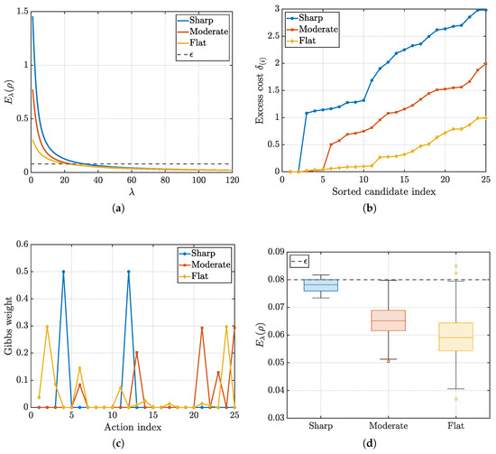
Figure 1 illustrates the geometry-dependent behavior of the relaxation error. Figure 1a shows the decay of ${\mathcal{E}}_{\lambda }\left(\rho \right)$ as a function of $\lambda$, highlighting that the rate of convergence depends strongly on the geometry of the excess-cost vector. Figure 1b displays the distribution of sorted excess costs in the three regimes, making explicit the differences in near-optimal mass. Figure 1c shows the corresponding Gibbs weights at the calibrated inverse temperature, illustrating how geometry affects the concentration pattern. Finally, Figure 1d reports the distribution of the relaxation errors across regimes at the common calibrated value ${\lambda }^{\ast }$, showing that flatter geometries yield smaller errors.

Figure 1. Experiment 1: geometry-dependent behavior of the entropic relaxation error across the three geometry regimes. (a) Relaxation error as a function of $\lambda$. Each curve corresponds to a representative cost vector from the sharp, moderate, and flat regimes, respectively. (b) Distribution of sorted excess costs ${\delta }_{\left(i\right)}$ in the three regimes. (c) Gibbs weights $p_i(\lambda ;\rho )$ computed at the calibrated inverse temperature $\lambda ={\lambda }^{\ast }$, for representative cost vectors in each regime, plotted over the action index. (d) Boxplots represent the distribution of the relaxation error ${\mathcal{E}}_{\lambda }\left(\rho \right)$ over the test set for each regime, with $\lambda ={\lambda }^{\ast }$ fixed.

These results show that the approximation error depends on the geometry of the excess-cost vector. In particular, larger near-optimal sets require smaller inverse temperatures to achieve a fixed tolerance, in agreement with the bounds in Section 4.

6.2. Experiment 2: Conformal Calibration of the Inverse Temperature

The second experiment evaluates the conformal calibration rule introduced in Section 5. The objective is to verify the empirical coverage guarantee and to compare the calibrated inverse temperature with several baseline selection rules in a contextual finite-action benchmark.

The data generation mechanism is contextual and geometry-controlled. Each instance consists of a context vector $x\in {\mathbb{R}}^d$ and an induced cost vector

$$\rho =({\rho }_1,\dots ,{\rho }_N),$$

with $d=6$ and $N=20$. Calibration, test, and oracle samples are all drawn from the same nominal mixture of three geometry regimes with probabilities

$$(0.34,0.33,0.33).$$

The three regimes are as follows:

• Isolated: one exact minimizer, one near-optimal competitor, and the remaining actions separated by intermediate-to-large excess costs.
• Few-near: one exact minimizer, four near-optimal competitors, and the remaining actions distributed over intermediate and far excess-cost ranges.
• Many-near: one exact minimizer, ten near-optimal competitors, and the remaining actions concentrated closer to the minimum.

After assigning one exact minimizer, the near-optimal, intermediate, and far excess costs are sampled from regime-dependent uniform ranges. The parameter values used in the experiment are as follows:

• Isolated: near range $[0.35,0.55]$, intermediate range $[0.90,1.60]$, far range $[1.80,3.20]$.
• Few-near: near range $[0.01,0.04]$, intermediate range $[0.20,0.55]$, far range $[0.65,1.40]$.
• Many-near: near range $[0.00,0.02]$, intermediate range $[0.03,0.10]$, far range $[0.10,0.35]$.

A small context-dependent perturbation is then added, after which the vector is recentered so that the minimum excess cost is zero and a common random offset is applied. Since the relaxation error is translation-invariant, this offset does not affect the operator-level calibration target.

Calibration is performed on a sample of size $n=800$, test evaluation uses 6000 independent instances, and the oracle reference uses a much larger calibration sample of size 15,000. The target miscoverage level is $\alpha =0.1$, the target tolerance is $\tau =0.06$, and the inverse temperature is selected over an adaptively enlarged search grid.

The following inverse temperature selection rules are compared:

• ProposedConf: the conformal calibration rule defined in (43).
• GlobalFixed: a single fixed inverse temperature obtained as the average of the regime-specific conformal temperatures estimated on the calibration set:

  $${\lambda }_{\mathrm{GlobalFixed}}={\displaystyle \frac{1}{R}}\sum _{r=1}^R{\lambda }_r^{\mathrm{conf}},R=3,$$

  where ${\lambda }_r^{\mathrm{conf}}$ denotes the conformal temperature obtained by applying the calibration rule to the subset of calibration instances belonging to regime r.
• MeanRisk: the smallest $\lambda$ on the search grid such that the empirical mean relaxation error on the calibration set satisfies

  $${\displaystyle \frac{1}{n}}\sum _{j=1}^n{\mathcal{E}}_{\lambda }\left({\rho }^{\left(j\right)}\right)\le \tau .$$
• WorstCase: the deterministic choice

  $${\lambda }_{\mathrm{WorstCase}}={\displaystyle \frac{logN}{\tau }},$$

  obtained from the worst-case bound (35). This rule does not use calibration data and is therefore expected to be conservative.
• OracleCal: the same conformal calibration rule applied to a much larger calibration sample, used only as a reference to approximate the large-sample calibration target.

Table 1 reports the empirical coverage and approximation accuracy obtained by the different methods. Here, $q_{0.95}$ Error denotes the empirical 95th percentile of the test relaxation error.

Table 1. Experiment 2: calibration results.

Method	Coverage	Mean Error	${\mathit{q}}_{0.95}$ Error
ProposedConf	1.00000	0.043074	0.059861
GlobalFixed	0.45867	0.062963	0.095184
MeanRisk	0.53333	0.059268	0.088470
WorstCase	1.00000	0.043155	0.060000
OracleCal	1.00000	0.043074	0.059861

Table 1 shows that ProposedConf attains full empirical coverage in this benchmark and coincides with OracleCal up to numerical precision. The corresponding upper-tail error remains at the target tolerance level. By contrast, GlobalFixed and MeanRisk fail to control the upper tail of the relaxation error and exhibit substantial undercoverage. WorstCase also attains full coverage, but in this benchmark its performance is nearly indistinguishable from that of the conformal selector.

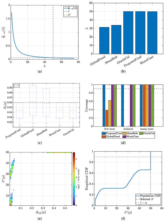
Figure 2 summarizes the behavior of the calibration procedure and the resulting performance. Figure 2a shows the empirical calibration curve ${\widehat{q}}_{1-\alpha }\left(\lambda \right)$, together with the tolerance level $\tau$ and the selected value ${\lambda }^{\ast }$. The monotonic decay of the curve and its intersection with $\tau$ illustrate the threshold structure underlying the conformal selection rule. Figure 2b reports the selected inverse temperatures for the different methods, showing that ProposedConf coincides with OracleCal and is numerically very close to the worst-case rule in this benchmark. Figure 2c displays the distribution of the test relaxation error for each method. The proposed calibration controls the upper tail of the error at the prescribed tolerance, whereas MeanRisk and GlobalFixed exhibit substantial violations. Figure 2d shows regime-wise coverage across methods. While ProposedConf maintains full coverage in all three regimes in this benchmark, GlobalFixed and MeanRisk exhibit marked heterogeneity across geometries. Figure 2e illustrates the relationship between the required inverse temperature and the top-two gap ${\Delta }_{\left(2\right)}\left(\rho \right)$, confirming that smaller gaps require larger values of $\lambda$, with additional variability induced by the near-optimal mass. Figure 2f shows the empirical distribution of the instance-wise required inverse temperatures. The selected value ${\lambda }^{\ast }$ corresponds to the smallest value achieving the target level $1-\alpha$, as predicted by the conformal calibration rule.

Figure 2. Experiment 2: empirical behavior of the conformal calibration rule in the contextual finite-action benchmark. (a) Calibration curve ${\widehat{q}}_{1-\alpha }\left(\lambda \right)$ computed on the pooled calibration sample. The horizontal line indicates the tolerance $\tau$ and the vertical line marks the selected value ${\lambda }^{\ast }$. (b) Selected inverse temperatures for the compared methods. (c) Boxplots of the test relaxation error ${\mathcal{E}}_{\lambda }\left(\rho \right)$ for the compared methods. The horizontal dashed line indicates the tolerance $\tau$. (d) Regime-wise test coverage for all methods. Calibration is performed on the pooled nominal mixture, and evaluation is stratified according to the test regime. (e) Instance-wise relationship between geometry and required inverse temperature. Each point corresponds to a cost vector $\rho$, and ${\lambda }^{\ast }\left(\rho \right)$ denotes the smallest value of $\lambda$ such that ${\mathcal{E}}_{\lambda }\left(\rho \right)\le \tau$. (f) Empirical cumulative distribution function of the instance-wise required inverse temperatures ${\lambda }^{\ast }\left(\rho \right)$ in the population. The vertical line indicates the selected conformal value ${\lambda }^{\ast }$, and the horizontal line marks the target level $1-\alpha$.

In this benchmark, the conformal selector is numerically very close to the deterministic worst-case rule. This can be stated more precisely in terms of the population distribution of the instance-wise thresholds $\Lambda \left(\rho \right)$ introduced in Definition 5. The deterministic rule ${\lambda }_{\mathrm{WorstCase}}=logN/\tau$ controls the tolerance for every cost vector and is attained, up to the asymptotic approximation of Section 4, by geometries with an isolated minimizer and a sufficiently separated near-optimal set, for which the relaxation error remains close to the worst-case scale $logN/\lambda$. The conformal selector provides a meaningful improvement over this deterministic rule only when the upper $(1-\alpha )$-quantile of $\Lambda \left(\rho \right)$ lies strictly below $logN/\tau$; that is, when such near-worst-case geometries occur with population probabilities smaller than $\alpha$. In the nominal mixture of Experiment 2, difficult geometries still carry enough mass for the upper-tail calibration target to remain near the worst-case value. By contrast, the additional mixture-sensitivity study reported in Table 2 shows that the selector moves away from the worst-case scale when the population is sufficiently concentrated on the many-near regime.

Table 2. Sensitivity of the conformal calibration rule to extreme nominal mixture weights in Experiment 2. Reported values are mean ± standard deviation over 10 independent realizations.

Mixture $({\mathit{p}}_{\mathbf{iso}},{\mathit{p}}_{\mathbf{few}},{\mathit{p}}_{\mathbf{many}})$	${\mathit{\lambda }}^{\ast }$	Coverage	Mean Error	${\mathit{q}}_{0.95}$ Error
$(0.34,0.33,0.33)$	$50.045\pm 0.000$	$1.0000\pm 0.0000$	$0.04298\pm 0.00032$	$0.05986\pm 0.00000$
$(0.85,0.10,0.05)$	$50.045\pm 0.000$	$1.0000\pm 0.0000$	$0.05642\pm 0.00011$	$0.05986\pm 0.00000$
$(0.05,0.10,0.85)$	$32.093\pm 1.144$	$0.8979\pm 0.0124$	$0.03654\pm 0.00075$	$0.08462\pm 0.01296$

To assess sensitivity to the nominal geometry mixture, we repeated the calibration experiment under two more extreme populations, namely $(0.85,0.10,0.05)$ and $(0.05,0.10,0.85)$, in addition to the baseline mixture $(0.34,0.33,0.33)$. In each case, calibration and test samples were drawn from the same mixture, the contextual generator and all numerical parameters were kept unchanged, and the experiment was repeated over 10 independent realizations. The resulting metrics are reported in Table 2. The observed pattern is asymmetric. When the population is shifted toward the isolated regime, the calibrated inverse temperature remains at the same value as in the baseline mixture, while the mean relaxation error increases. By contrast, when the population is strongly shifted toward the many-near regime, the calibrated inverse temperature decreases from $50.045$ to $32.093\pm 1.144$, and the empirical coverage moves close to the target level $1-\alpha =0.9$. Thus, in the present benchmark, the conformal selector remains at the near-worst-case scale as long as the upper-tail calibration target is dominated by difficult geometries, and decreases only when the geometry distribution is sufficiently concentrated on broad near-optimal sets. The reported $q_{0.95}$ values are included only as an auxiliary diagnostic, since the conformal calibration target is the upper $(1-\alpha )$-quantile rather than the $0.95$ quantile.

The conformal guarantee relies on the exchangeability of calibration and test samples. To assess the effect of violating this assumption, we perform an additional experiment in which calibration and test data are drawn from different geometry regimes.

We consider shifted scenarios in which the calibration sample is drawn from a single regime, while the test sample is drawn from a different regime or from the nominal mixture. All other aspects of the setup are unchanged.

Table 3 reports the resulting coverage and approximation error. The results exhibit a clear and systematic pattern. When calibration is performed on geometries that are at least as challenging as those encountered at test time (for example, isolated → many-near), the method remains conservative and continues to satisfy the tolerance constraint. In contrast, when calibration is performed on more difficult geometries and evaluation is carried out on simpler ones (many-near → isolated), the selected inverse temperature becomes too small, leading to a substantial increase in the relaxation error and a collapse in coverage.

Table 3. Effect of distribution shift on conformal calibration. Calibration and test samples are drawn from different geometry regimes.

Scenario	Coverage	Mean Error	${\mathit{q}}_{0.95}$ Error
nominal → nominal	1.00	0.043	0.060
isolated → many-near	1.00	0.025	0.033
many-near → isolated	0.00	0.520	0.526
isolated → few-near	1.00	0.043	0.050
many-near → nominal	0.30	0.271	0.526

These results are consistent with the theoretical analysis. In particular, the inverse temperature required to achieve a prescribed tolerance depends on the geometry of the excess-cost vector. Under distribution shift, the calibrated value may fail to control the upper tail of the relaxation error.

From a computational viewpoint, the proposed method separates an offline calibration stage from the online decision stage. In the straightforward implementation used here, calibrating over n cost vectors, an action dimension K, and a grid of m candidate inverse temperatures requires $O\left(mnK\right)$ operations to evaluate the relaxation errors and $O(mnlogn)$ operations to compute the empirical upper quantile by sorting at each grid point. Once ${\lambda }^{\ast }$ has been selected, deployment uses a fixed inverse temperature and the online cost reduces to the standard Gibbs evaluation, namely $O\left(K\right)$ per decision, which is of the same order as for a fixed-temperature baseline. The geometric descriptors introduced in the analysis are not required at deployment time. Table 4 reports representative MATLAB wall-clock timings as the action dimension varies. Wall-clock times were measured in MATLAB on a Windows 64-bit machine equipped with an AMD Ryzen 9 8945HS processor (4.00 GHz) and 32 GB RAM. Reported values correspond to mean ± standard deviation over five independent runs, and online timings are normalized per decision using batches of ${10}^5$ decisions. The results show that the calibration stage grows with the action dimension, whereas the online cost of ProposedConf remains essentially indistinguishable from that of the fixed-temperature baseline.

Table 4. Computational overhead of the conformal calibration module as a function of the action dimension K. Reported values are mean ± standard deviation over 5 independent runs.

K	Calibration Time (s)	Online Time/Decision (μs), ProposedConf	Online Time/Decision (μs), Fixed Baseline
10	$0.440\pm 0.020$	$0.232\pm 0.013$	$0.213\pm 0.003$
20	$0.680\pm 0.009$	$0.302\pm 0.008$	$0.315\pm 0.004$
50	$0.962\pm 0.016$	$0.583\pm 0.014$	$0.616\pm 0.008$
100	$1.820\pm 0.021$	$0.968\pm 0.020$	$1.052\pm 0.028$
200	$2.875\pm 0.021$	$1.708\pm 0.034$	$1.866\pm 0.017$

6.3. Experiment 3: Contextual Bandit with Sequential Risk

The third experiment studies the proposed calibration rule in a sequential decision setting. The goal is to assess how the calibrated inverse temperature affects both operator-level accuracy and downstream risk when action values are estimated.

The purpose of this experiment is illustrative rather than theorem-proving at the decision level. In particular, the conformal guarantee developed in Section 5 applies to the operator-level approximation error of the entropic relaxation and does not directly yield a bound on cumulative reward or long-term regret. Establishing such a link in multi-step decision problems would require additional assumptions on the environment dynamics, the propagation of value-estimation errors, and the sensitivity of the induced policy to approximation errors. Experiment 3 is formulated as a one-step contextual bandit with sequential risk, where downstream metrics describe how operator-level calibration is reflected in the induced decision behavior.

We consider a contextual finite-action bandit with one-step sequential risk. Each instance is defined by a context vector

$$x\in {\mathbb{R}}^d,d=5,$$

and an associated estimated action-value vector

$$\widehat{Q}(x,·)=\left(\widehat{Q}(x,1),\dots ,\widehat{Q}(x,K)\right),K=6.$$

The corresponding cost vector is defined by

$${\rho }_a\left(x\right)=-\widehat{Q}(x,a),a=1,\dots ,K.$$

The policy induced by inverse temperature $\lambda$ is the Gibbs policy

$${\pi }_{\lambda }(a\mid x)={\displaystyle \frac{exp\left(-\lambda {\rho }_a\left(x\right)\right)}{{\sum }_{b=1}^{K}exp\left(-\lambda {\rho }_b\left(x\right)\right)}}.$$

(47)

Larger values of $\lambda$ yield a sharper policy, whereas smaller values yield a more diffuse one.

The six actions are organized into three semantic groups. Action 1 is a safe action, actions 2 and 3 are risky actions, and actions 4–6 are distractor actions with clearly inferior value in most contexts. The data-generating mechanism is a mixture of three geometry regimes with probabilities

$$(0.35,0.40,0.25):$$

• Safe-dominant: the safe action is clearly optimal and the risky actions are suboptimal but still competitive;
• Ambiguous-risk: a risky action appears slightly better than the safe action and the top gaps are small, so the local geometry is difficult and fragile;
• Flat: several actions are nearly tied, creating a broad near-optimal set.

For reproducibility, the distributions of the ground-truth action values $Q^{\star }(x,·)$ are specified explicitly for each regime.

In the safe-dominant regime, the safe action has the highest expected value, while risky actions are suboptimal:

$$Q_1^{\star }\sim \mathcal{N}(1.10,0.{10}^2),Q_{2,3}^{\star }\sim \mathcal{N}(0.90,0.{06}^2),Q_{4:6}^{\star }\sim \mathcal{N}(0.40,0.{08}^2).$$

In the ambiguous-risk regime, risky actions are competitive or slightly optimistic:

$$Q_1^{\star }\sim \mathcal{N}(1.00,0.{03}^2),Q_2^{\star }\sim \mathcal{N}(1.05,0.{03}^2),Q_3^{\star }\sim \mathcal{N}(1.01,0.{03}^2),$$

while the remaining actions have lower values:

$$Q_{4:6}^{\star }\sim \mathcal{N}(0.55,0.{08}^2).$$

In the flat regime, several actions are nearly tied:

$$Q_1^{\star }\sim \mathcal{N}(1.00,0.{03}^2),Q_2^{\star }\sim \mathcal{N}(0.99,0.{03}^2),Q_3^{\star }\sim \mathcal{N}(0.98,0.{03}^2),$$

with remaining actions taking smaller values:

$$Q_4^{\star }\sim \mathcal{N}(0.95,0.{03}^2),Q_{5,6}^{\star }\sim \mathcal{N}(0.55,0.{06}^2).$$

For each instance, a true action-value vector $Q^{\star }(x,·)$ is sampled according to the regime, and a noisy estimate $\widehat{Q}(x,·)$ is constructed by adding Gaussian noise with larger variance and positive bias on the risky actions, modeling optimistic overestimation.

The outcome of a selected action is realized rather than averaged deterministically. Safe and distractor actions return their nominal value, whereas risky actions produce either a positive outcome or an adverse event with regime-dependent probability. In particular, risky actions incur a higher failure probability when their nominal value exceeds one, and adverse realizations yield a substantial negative reward. Consequently, the inverse temperature directly affects risk exposure through policy concentration.

Calibration, test, and oracle samples contain

$$n_{\mathrm{cal}}=800,n_{\mathrm{test}}=6000,n_{\mathrm{oracle}}=15000$$

instances, respectively. The target miscoverage level is $\alpha =0.1$, the target tolerance is $\tau =0.06$, and inverse temperatures are searched over the grid

$$\lambda \in [1,120].$$

The compared inverse-temperature selection rules are the following:

• ProposedConf: the conformal selector defined in (43);
• FixedSoftmax: a fixed practical baseline with $\lambda =12$;
• MeanRisk: the smallest grid value such that the empirical mean relaxation error on the calibration set is at most $\tau$;
• WorstCase: the deterministic rule $\lambda =log\left(K\right)/\tau$ derived from the worst-case bound;
• OracleCal: the conformal selector computed on a much larger calibration set;
• Greedy: the limiting sharply concentrated policy, approximated numerically by $\lambda ={10}^6$.

The experiment is repeated over 25 independent random seeds, with independently generated calibration and test samples in each run. Reported results correspond to multi-seed averages together with their standard deviations.

Both operator-level and decision-level metrics are considered. Operator-level metrics include empirical coverage, mean relaxation error, and $q_{0.95}\left(E_{\lambda }\right)$. Decision-level metrics include mean realized return, adverse-event rate, average probability assigned to the true best action, and risky-action usage frequency.

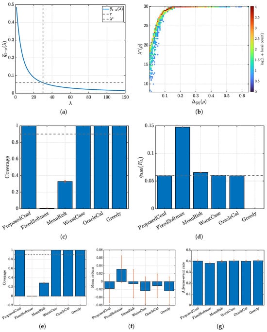
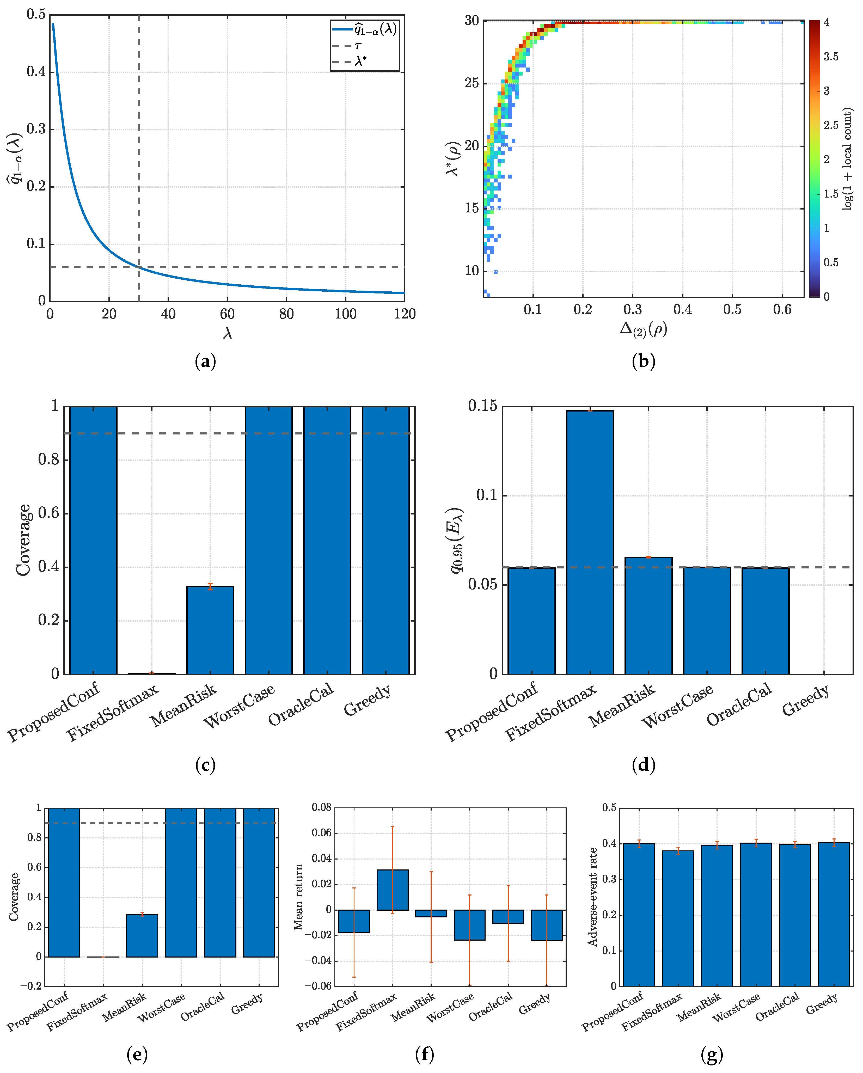
Table 5 and Figure 3 show that ProposedConf maintains operator-level validity in the risky contextual setting. The upper-tail error remains at the target threshold, whereas MeanRisk and FixedSoftmax fail to control the upper tail. The selected conformal inverse temperature is stable across seeds and coincides with the oracle reference in this experiment:

$${\lambda }_{\mathrm{conf}}=30.094,{\lambda }_{\mathrm{oracle}}=30.094.$$

This indicates that the conformal selector closely tracks the large-sample calibration target. Figure 3a shows a representative calibration curve ${\widehat{q}}_{1-\alpha }\left(\lambda \right)$ in the contextual setting. The monotonic decay and its intersection with the tolerance $\tau$ illustrate the threshold structure of the conformal selection rule. Figure 3b displays the instance-wise relationship between the required inverse temperature and the top-two gap ${\Delta }_{\left(2\right)}\left(\rho \right)$, confirming that calibration difficulty remains strongly geometry-dependent. Figure 3c,d report global operator-level metrics across seeds. ProposedConf maintains the desired coverage while controlling the upper-tail error at the prescribed level, whereas MeanRisk and FixedSoftmax exhibit clear violations. Figure 3e–g focus on the ambiguous-risk regime. They show that ProposedConf preserves operator-level validity while avoiding the overcommitment exhibited by the greedy policy. In contrast, FixedSoftmax achieves higher return only by violating the operator-level constraint.

Table 5. Experiment 3: multi-seed global results for the contextual bandit with sequential risk. Reported values are mean ± standard deviation over 25 random seeds.

Method	Coverage	${\mathit{q}}_{0.95}\left({\mathit{E}}_{\mathit{\lambda }}\right)$	Mean Return	Adverse Rate
ProposedConf	$1.000\pm 0.000$	$0.05954\pm 0.00000$	$0.254\pm 0.018$	$0.304\pm 0.005$
FixedSoftmax	$0.0049\pm 0.0009$	$0.14771\pm 0.00009$	$0.284\pm 0.017$	$0.291\pm 0.005$
MeanRisk	$0.328\pm 0.011$	$0.06561\pm 0.00032$	$0.256\pm 0.020$	$0.303\pm 0.006$
WorstCase	$1.000\pm 0.000$	$0.06000\pm 0.00000$	$0.252\pm 0.021$	$0.304\pm 0.007$
OracleCal	$1.000\pm 0.000$	$0.05954\pm 0.00000$	$0.259\pm 0.020$	$0.302\pm 0.006$
Greedy	$1.000\pm 0.000$	$0.00000\pm 0.00000$	$0.245\pm 0.019$	$0.308\pm 0.006$

Figure 3. Experiment 3: contextual bandit with sequential risk. Calibration curve, geometry-dependent inverse temperature, and operator- and decision-level performance across regimes. (a) Representative conformal calibration curve ${\widehat{q}}_{1-\alpha }\left(\lambda \right)$ in the risky contextual setting. The horizontal line marks the tolerance $\tau$, and the vertical line marks the selected ${\lambda }^{\ast }$. (b) Instance-wise geometry-to-calibration relationship: required inverse temperature ${\lambda }^{\ast }\left(\rho \right)$ versus top-two gap ${\Delta }_{\left(2\right)}\left(\rho \right)$. (c) Multi-seed global operator-level coverage. Error bars show one standard deviation across seeds. (d) Multi-seed global upper-tail operator error $q_{0.95}\left(E_{\lambda }\right)$. Error bars show one standard deviation across seeds. (e) Multi-seed metrics restricted to the ambiguous-risk regime: coverage. (f) Multi-seed metrics restricted to the ambiguous-risk regime: mean return. (g) Multi-seed metrics restricted to the ambiguous-risk regime: adverse-event rate.

Thus, the proposed rule is not a procedure designed to maximize return. Its role is to calibrate the sharpness of the induced Gibbs policy through operator-level control of the relaxation error. In the present experiment, this effect at the operator level translates into only moderate differences in adverse event rate, since the considered noise and failure regime does not produce large changes in exposure to risky actions across methods. Accordingly, the main conclusion is not that geometry-aware calibration uniformly improves downstream performance, but that it preserves the prescribed operator-level validity while interacting in a transparent way with the induced decision policy. Larger separations in realized return or adverse event frequency would be expected in regimes with stronger optimistic bias, higher estimation noise, or more pronounced asymmetry in the failure probabilities of the risky actions. A mathematical transfer from operator-level tolerance control to cumulative reward or long-term regret in multi-step decision problems is not established in the present analysis.

7. Concluding Remarks

This study investigated inverse-temperature calibration for entropic soft-min operators from a geometry-aware perspective. The analysis shows that the approximation error depends on the geometry of the excess-cost vector rather than only on support size.

Geometry-dependent bounds were derived to characterize how descriptors such as the top-two gap and the near-optimal mass affect the approximation accuracy. These results show that the inverse temperature required to achieve a given tolerance varies across populations with different near-optimal geometries.

A conformal calibration rule was introduced to select the inverse temperature with finite-sample distribution-free validity under exchangeability. The method selects the smallest value ensuring that a prescribed upper quantile of the relaxation error satisfies the target tolerance.

The numerical experiments are consistent with the theoretical analysis. The geometry-controlled benchmark shows the dependence of the relaxation error on the excess-cost geometry. The calibration experiments confirm that the proposed method attains the desired marginal coverage while avoiding the conservativeness of worst-case bounds and the failure of mean-based rules. The contextual bandit experiment shows that the same geometric dependence persists when the soft-min operator induces a decision policy.

The results indicate that inverse-temperature selection should be treated as a geometry-dependent calibration problem. The proposed method provides a principled and reproducible alternative to heuristic tuning rules.

The validity of the method depends on the geometry distribution represented in the calibration sample. Under distribution shift, the selected inverse temperature may fail to control the upper tail of the relaxation error. This reflects the role of exchangeability in the conformal guarantee.

The present framework is formulated at the population level, relies on the exchangeability assumption underlying the conformal guarantee, and develops its geometric analysis under the assumption of uniform weights. Extending the geometric descriptors and the associated bounds to weighted soft-min relaxations, where quantities such as the weighted near-optimal mass replace descriptors based on cardinality, remains an open direction, together with calibration depending on covariates, settings beyond exchangeability, and adaptive decision systems. In particular, dynamic multistep reinforcement learning problems introduce temporal dependence, distribution shift induced by the policy, and an additional gap between operator-level approximation error and long-term decision risk. Establishing a mathematical transfer from calibrated soft-min error control to cumulative reward or regret in such settings remains an open direction for future work.

Likewise, embedding the present calibration scheme into standard multi-step reinforcement learning benchmarks such as Atari or MuJoCo would require fixing additional algorithmic choices concerning representation learning, policy optimization, exploration, and training dynamics. Such an evaluation is therefore left for future work.

Relatedly, integrating the present calibration rule with annealing schedules or learnable-temperature mechanisms within full reinforcement learning pipelines also remains a natural direction for future work.

More broadly, richer hierarchical decision architectures provide a natural application scenario for future extensions of the present framework. Recent application-oriented work on large language model-guided hierarchical games for intelligent battery coordination illustrates this broader class of settings [46].

References

- Nesterov, Y. Smooth minimization of non-smooth functions. Math. Program. 2005, 103, 127–152. [Google Scholar] [CrossRef] [Scilit]
- Boyd, S.; Vandenberghe, L. Convex Optimization; Number Pt. 1 in Berichte Über Verteilte Messysteme; Cambridge University Press: Cambridge, UK, 2004; Available online: https://books.google.es/books?id=mYm0bLd3fcoC (accessed on 16 March 2026).
- Nishioka, A.; Kanno, Y. A feasible smoothing accelerated projected gradient method for nonsmooth convex optimization. Oper. Res. Lett. 2024, 57, 107181. [Google Scholar] [CrossRef] [Scilit]
- Palomar, D.P. Convex Optimization Theory. In Portfolio Optimization: Theory and Application; Cambridge University Press: Cambridge, UK, 2025; pp. 491–538. Available online: https://portfoliooptimizationbook.com/slides/slides-convex-optimization-theory.pdf (accessed on 16 March 2026).
- Blanchard, P.; Higham, D.J.; Higham, N.J. Accurately computing the log-sum-exp and softmax functions. IMA J. Numer. Anal. 2020, 41, 2311–2330. [Google Scholar] [CrossRef] [Scilit]
- Calafiore, G.C.; Gaubert, S.; Possieri, C. Log-Sum-Exp Neural Networks and Posynomial Models for Convex and Log-Log-Convex Data. IEEE Trans. Neural Netw. Learn. Syst. 2020, 31, 827–838. [Google Scholar] [CrossRef] [Scilit]
- Zhang, S.; Tepedelenlioğlu, C.; Banavar, M.K.; Spanias, A. Max-consensus using the soft maximum. In Proceedings of the 2013 Asilomar Conference on Signals, Systems and Computers, Pacific Grove, CA, USA, 3–7 November 2013; pp. 433–437. [Google Scholar] [CrossRef] [Scilit]
- Nowzari, A.; Rabbat, M.G. Improved Bounds for Max Consensus in Wireless Networks. IEEE Trans. Signal Inf. Process. Netw. 2019, 5, 305–319. [Google Scholar] [CrossRef] [Scilit]
- Wainwright, M.J.; Jordan, M.I. Graphical Models, Exponential Families, and Variational Inference. Found. Trends Mach. Learn. 2008, 1, 1–305. [Google Scholar] [CrossRef] [Scilit]
- Cover, T.M.; Thomas, J.A. Elements of Information Theory, 2nd ed.; John Wiley & Sons: Hoboken, NJ, USA, 2006. [Google Scholar] [CrossRef] [Scilit]
- Cuturi, M. Sinkhorn distances: Lightspeed computation of optimal transport. In Proceedings of the 27th International Conference on Neural Information Processing Systems-Volume 2, Lake Tahoe, NV, USA, 5–10 December 2013; NIPS’13. pp. 2292–2300. [Google Scholar] [CrossRef] [Scilit]
- Lefebvre, T.; Crevecoeur, G. On Entropy Regularized Path Integral Control for Trajectory Optimization. Entropy 2020, 22, 1120. [Google Scholar] [CrossRef] [Scilit]
- Lefebvre, T.; Crevecoeur, G. Entropy Regularised Deterministic Optimal Control: From Path Integral Solution to Sample-Based Trajectory Optimisation. In Proceedings of the 2022 IEEE/ASME International Conference on Advanced Intelligent Mechatronics (AIM); IEEE Press: Piscataway, NJ, USA, 2022; pp. 401–408. [Google Scholar] [CrossRef] [Scilit]
- Williams, G.; Drews, P.; Goldfain, B.; Rehg, J.M.; Theodorou, E.A. Aggressive driving with model predictive path integral control. In Proceedings of the 2016 IEEE International Conference on Robotics and Automation (ICRA), Stockholm, Sweden, 16–21 May 2016; pp. 1433–1440. [Google Scholar] [CrossRef] [Scilit]
- Xu, H.; Xuan, J.; Zhang, G.; Lu, J. Trust region policy optimization via entropy regularization for Kullback–Leibler divergence constraint. Neurocomputing 2024, 589, 127716. [Google Scholar] [CrossRef] [Scilit]
- Tao, F.; Wu, M.; Cao, Y. Generalized Maximum Entropy Reinforcement Learning via Reward Shaping. IEEE Trans. Artif. Intell. 2024, 5, 1563–1572. [Google Scholar] [CrossRef] [Scilit]
- Bhole, A.; Filabadi, M.M.; Crevecoeur, G.; Lefebvre, T. Unifying Entropy Regularization in Optimal Control: From and Back to Classical Objectives via Iterated Soft Policies and Path Integral Solutions. arXiv 2025, arXiv:2512.06109. [Google Scholar] [CrossRef] [Scilit]
- Arriojas, A.; Adamczyk, J.; Tiomkin, S.; Kulkarni, R.V. Entropy Regularized Reinforcement Learning Using Large Deviation Theory. Phys. Rev. Res. 2023, 5, 023085. [Google Scholar] [CrossRef] [Scilit]
- Labbi, S.; Mangold, P.; Tiapkin, D.; Moulines, E. On Global Convergence Rates for Federated Softmax Policy Gradient under Heterogeneous Environments. In Proceedings of the 29th International Conference on Artificial Intelligence and Statistics, Tangier, Morocco, 2–5 May 2026; Available online: https://openreview.net/forum?id=aPAq9U7MFm (accessed on 16 March 2026).
- Vovk, V.; Gammerman, A.; Shafer, G. Algorithmic Learning in a Random World, 2nd ed.; Springer: Cham, Switzerland, 2022. [Google Scholar] [CrossRef] [Scilit]
- Lei, J.; G’Sell, M.; Rinaldo, A.; Tibshirani, R.J.; Wasserman, L. Distribution-Free Predictive Inference for Regression. J. Am. Stat. Assoc. 2018, 113, 1094–1111. [Google Scholar] [CrossRef] [Scilit]
- Balasubramanian, V.N.; Ho, S.S.; Vovk, V. Conformal Prediction for Reliable Machine Learning: Theory, Adaptations and Applications; Morgan Kaufmann: San Francisco, CA, USA, 2014. [Google Scholar] [CrossRef] [Scilit]
- Romano, Y.; Patterson, E.; Candes, E. Conformalized Quantile Regression. In Proceedings of the Advances in Neural Information Processing Systems; Wallach, H., Larochelle, H., Beygelzimer, A., d’Alché-Buc, F., Fox, E., Garnett, R., Eds.; Curran Associates, Inc.: Red Hook, NY, USA, 2019; Volume 32, Available online: https://proceedings.neurips.cc/paper_files/paper/2019/file/5103c3584b063c431bd1268e9b5e76fb-Paper.pdf (accessed on 16 March 2026).
- Zhou, X.; Chen, B.; Gui, Y.; Cheng, L. Conformal Prediction: A Data Perspective. arXiv 2025, arXiv:2410.06494. [Google Scholar] [CrossRef] [Scilit]
- Cortes-Gomez, S.; Patiño, C.; Byun, Y.; Wu, S.; Horvitz, E.; Wilder, B. Utility-Directed Conformal Prediction: A Decision-Aware Framework for Actionable Uncertainty Quantification. arXiv 2025, arXiv:2410.01767. [Google Scholar] [CrossRef] [Scilit]
- Yeh, C.; Christianson, N.; Wierman, A.; Yue, Y. Conformal Risk Training: End-to-End Optimization of Conformal Risk Control. arXiv 2025, arXiv:2510.08748. [Google Scholar] [CrossRef] [Scilit]
- Huang, H.; Sharma, S.; Loquercio, A.; Angelopoulos, A.; Goldberg, K.; Malik, J. Conformal Policy Learning for Sensorimotor Control under Distribution Shifts. In Proceedings of the 2024 IEEE International Conference on Robotics and Automation (ICRA), Yokohama, Japan, 13–17 May 2024; pp. 16285–16291. [Google Scholar] [CrossRef] [Scilit]
- Flovik, V. Quantifying Distribution Shifts and Uncertainties for Enhanced Model Robustness in Machine Learning Applications. arXiv 2024, arXiv:2405.01978. [Google Scholar] [CrossRef] [Scilit]
- Lin, V.; Jang, K.J.; Dutta, S.; Caprio, M.; Sokolsky, O.; Lee, I. DC4L: Distribution shift recovery via data-driven control for deep learning models. In Proceedings of the 6th Annual Learning for Dynamics & Control Conference; Abate, A., Cannon, M., Margellos, K., Papachristodoulou, A., Eds.; PMLR: Cambridge, MA, USA, 2024; Volume 242, pp. 1526–1538. Available online: https://proceedings.mlr.press/v242/lin24b.html (accessed on 16 March 2026).
- Danesh, M.H.; Wabartha, M.; Pineau, J.; Lin, H.C. Mitigating Distribution Shifts: Uncertainty-Aware Offline-to-Online Reinforcement Learning. 2025. Available online: https://openreview.net/forum?id=0WqAnYWi7H (accessed on 1 March 2026).
- Ellis, R.S. Entropy, Large Deviations, and Statistical Mechanics; Grundlehren der mathematischen Wissenschaften; Springer: New York, NY, USA, 1985. [Google Scholar] [CrossRef] [Scilit]
- Amari, S.I. Information Geometry and Its Applications; Applied Mathematical Sciences; Springer: Tokyo, Japan, 2016. [Google Scholar] [CrossRef] [Scilit]
- Donsker, M.D.; Varadhan, S.R.S. Asymptotic evaluation of certain markov process expectations for large time, I. Commun. Pure Appl. Math. 1975, 28, 1–47. [Google Scholar] [CrossRef] [Scilit]
- Dembo, A.; Zeitouni, O. Large Deviations Techniques and Applications, 2nd ed.; Stochastic Modelling and Applied Probability; Springer: Berlin/Heidelberg, Germany, 2009. [Google Scholar] [CrossRef] [Scilit]
- Dupuis, P.; Ellis, R.S. A Weak Convergence Approach to the Theory of Large Deviations; Wiley Series in Probability and Statistics; John Wiley & Sons: Hoboken, NJ, USA, 1997. [Google Scholar] [CrossRef] [Scilit]
- Hartmann, C.; Richter, L.; Schütte, C.; Zhang, W. Variational Characterization of Free Energy: Theory and Algorithms. Entropy 2017, 19, 626. [Google Scholar] [CrossRef] [Scilit]
- Wong, R. Asymptotic Approximations of Integrals; Academic Press: Cambridge, MA, USA, 1989. [Google Scholar] [CrossRef] [Scilit]
- de Bruijn, N. Asymptotic Methods in Analysis; Bibliotheca Mathematica; Dover Publications: Garden City, NY, USA, 1981; Available online: https://books.google.es/books?id=_tnwmvHmVwMC (accessed on 16 March 2026).
- Temme, N.M. Uniform asymptotic methods for integrals. Indag. Math. 2013, 24, 739–765. [Google Scholar] [CrossRef] [Scilit]
- Oliveira, R.I.; Orenstein, P.; Ramos, T.; Romano, J.V. Split Conformal Prediction and Non-Exchangeable Data. J. Mach. Learn. Res. 2022, 25, 1–38. [Google Scholar]
- Tibshirani, R.J.; Foygel Barber, R.; Candes, E.; Ramdas, A. Conformal Prediction Under Covariate Shift. In Proceedings of the Advances in Neural Information Processing Systems; Wallach, H., Larochelle, H., Beygelzimer, A., d’Alché-Buc, F., Fox, E., Garnett, R., Eds.; Curran Associates, Inc.: Red Hook, NY, USA, 2019; Volume 32, Available online: https://proceedings.neurips.cc/paper_files/paper/2019/file/8fb21ee7a2207526da55a679f0332de2-Paper.pdf (accessed on 16 March 2026).
- Xu, C.; Xie, Y. Conformal prediction interval for dynamic time-series. In Proceedings of the 38th International Conference on Machine Learning; Proceedings of Machine Learning Research; Meila, M., Zhang, T., Eds.; PMLR: Cambridge, MA, USA, 2021; Volume 139, pp. 11559–11569. Available online: https://proceedings.mlr.press/v139/xu21h.html (accessed on 16 March 2026).
- Zaffran, M.; Feron, O.; Goude, Y.; Josse, J.; Dieuleveut, A. Adaptive Conformal Predictions for Time Series. In Proceedings of the 39th International Conference on Machine Learning; Proceedings of Machine Learning Research; Chaudhuri, K., Jegelka, S., Song, L., Szepesvari, C., Niu, G., Sabato, S., Eds.; PMLR: Cambridge, MA, USA, 2022; Volume 162, pp. 25834–25866. Available online: https://proceedings.mlr.press/v162/zaffran22a.html (accessed on 16 March 2026).
- Vovk, V.; Nouretdinov, I.; Gammerman, A. Conformal e-testing. Pattern Recognit. 2025, 168, 111841. [Google Scholar] [CrossRef] [Scilit]
- Angelopoulos, A.N.; Barber, R.; Bates, S. Online conformal prediction with decaying step sizes. In Proceedings of the 41st International Conference on Machine Learning; Proceedings of Machine Learning Research; Salakhutdinov, R., Kolter, Z., Heller, K., Weller, A., Oliver, N., Scarlett, J., Berkenkamp, F., Eds.; PMLR: Cambridge, MA, USA, 2024; Volume 235, pp. 1616–1630. Available online: https://proceedings.mlr.press/v235/angelopoulos24a.html (accessed on 16 March 2026).
- Zou, Y.; Lin, Z.; Zhang, Q.; Liu, Z.; Xu, Z. Large language models enable semantic-guided hierarchical games for intelligent battery coordination. Adv. Eng. Inform. 2026, 71, 104312. [Google Scholar] [CrossRef] [Scilit]
Disclaimer/Publisher’s Note: The statements, opinions and data contained in all publications are solely those of the individual author(s) and contributor(s) and not of MDPI and/or the editor(s). MDPI and/or the editor(s) disclaim responsibility for any injury to people or property resulting from any ideas, methods, instructions or products referred to in the content. |
© 2026 by the authors. Licensee MDPI, Basel, Switzerland. This article is an open access article distributed under the terms and conditions of the Creative Commons Attribution (CC BY) license.