


Abstract
Mixed-signal simulation is indispensable for verifying modern integrated circuits that tightly couple analog and digital subsystems, yet the field lacks a unified framework for systematically comparing its diverse methodologies. This paper addresses that gap by proposing a novel three-axis taxonomy that classifies simulation methods along abstraction level, solver methodology, and analysis type, together with a comparative evaluation framework based on five quantitative metrics: accuracy, throughput, capacity, convergence reliability, and scalability. Applying this framework, we systematically compare thirteen classical method categories—spanning SPICE, FastSPICE, RF/periodic steady-state, behavioral modeling, co-simulation, and model order reduction—and eight AI/ML approaches including Gaussian process surrogates, graph neural networks, physics-informed neural networks, Bayesian optimization, and reinforcement learning. Our analysis reveals a clear maturity stratification: classical methods remain the only signoff-accurate approaches, Bayesian optimization represents the most industrially validated AI contribution with integration across all three major EDA platforms, while Neural ODE solvers and LLM-based design tools remain at the research stage. We identify a persistent academic-to-industry gap driven by foundry model complexity, limited benchmark diversity, and topology-specific overfitting. The proposed taxonomy and comparative framework provide practitioners with structured guidance for simulation method selection and highlight specific research directions needed to bridge the gap between AI promise and industrial deployment.
1. Introduction
Mixed-signal integrated circuits (ICs), combining analog and digital processing on a single die, are fundamental to modern electronics—from 5G transceivers [1] and IoT sensor interfaces [2] to automotive radar front-ends [3] and high-speed data converters [4]. The sustained growth of the analog and mixed-signal IC market [5], driven by increasing integration density, intensifies demand for simulation tools spanning the full analog/mixed-signal (AMS) design space.
Mixed-signal design complexity has grown substantially with technology scaling. At advanced nodes—FinFET, gate-all-around (GAA) transistors, and sub-3 nm geometries—effects such as self-heating, quantum tunneling, and increased process variability require device models of greater complexity [6,7]. Compact models like BSIM-CMG now require hundreds of parameters across process, voltage, and temperature (PVT) corners [6], while verification must address functional correctness and statistical yield [8]. Full transistor-level simulation of a modern AMS system-on-chip (SoC) can require days to weeks [9], motivating hierarchical and multi-abstraction strategies.
Simulation is the primary pre-silicon verification means in the AMS domain, where re-spin costs reach tens of millions of dollars. Different abstraction levels serve complementary roles: SPICE [10] provides the highest fidelity, behavioral models in Verilog-AMS or VHDL-AMS [8,11] enable system-level exploration, and real number modeling (RNM) offers digital-like speed [12]. However, no single approach satisfies accuracy, speed, and capacity simultaneously—a fundamental trilemma defining the AMS simulation landscape [9].
The evolution of mixed-signal simulation spans five decades (Figure 1). In 1973, Nagel and Pederson developed SPICE at UC Berkeley [10], establishing modified nodal analysis (MNA) and Newton–Raphson iteration as the foundational framework. SPICE2 (1975) introduced sparse matrix techniques enabling practical simulation [13]. The 1980s brought commercialization, with HSPICE introducing proprietary convergence enhancements and foundry-certified models [14]. The 1990s saw FastSPICE bridge the circuit-size gap [15] and standardized behavioral languages make co-simulation practical [11,16]. The 2000s brought SystemC-AMS [17] for architectural exploration and maturation of model order reduction (MOR) [18]. The 2010s introduced RNM for digital-centric verification [12]. The 2020s have seen a surge in AI-enhanced methods: graph neural networks for circuit prediction [19], reinforcement learning for topology synthesis [20], advanced Bayesian optimization [21], and large language models (LLMs) for EDA [22], though industrial maturity varies widely.
Figure 1.
Timeline of major milestones in mixed-signal simulation technology spanning five decades, from the original SPICE development at UC Berkeley in 1973 to contemporary AI-enhanced approaches.
Prior surveys have addressed aspects of this field. Gielen and Rutenbar [23] reviewed CAD for AMS circuits but predated machine learning (ML) in electronic design automation (EDA). Huang et al. [24] surveyed ML across EDA without examining mixed-signal simulation in depth. Recent works addressed ML for analog design [19,20] but not the complete simulation landscape. Critically, no existing work provides a unified taxonomic framework for systematically comparing the full spectrum of mixed-signal simulation methods—from classical SPICE algorithms to contemporary AI-enhanced approaches—using consistent evaluation criteria.
It is important to note that this paper is a review article: it does not propose a new simulation method or report original experimental results. Rather, its contribution lies in providing a systematic classification and comparative evaluation of existing methods based on published literature, vendor documentation, and reported benchmarks.
This paper addresses that gap with the following original contributions:
- A novel three-axis classification framework organizing mixed-signal simulation methods by abstraction level, solver methodology, and analysis type, providing a structured basis for systematic comparison.
- A comparative evaluation methodology based on five quantitative metrics (accuracy, throughput, capacity, convergence reliability, scalability) applied consistently across all method categories.
- A systematic comparative analysis of thirteen classical method categories and eight AI/ML approaches, yielding evidence-based maturity assessments and industrial readiness evaluations.
- Identification of specific research gaps and industrial deployment barriers through cross-cutting analysis of the method landscape.
The remainder of this paper is organized as follows. Section 2 presents the proposed taxonomy and evaluation framework. Section 3 applies the framework to classical simulation methods. Section 4 evaluates AI-enhanced methods. Section 5 presents the systematic comparison and analysis. Section 6 discusses implications, challenges, and future directions. Section 7 concludes.
2. Proposed Taxonomy and Evaluation Framework
This section presents the core methodological contribution of this paper: a three-axis taxonomy for classifying mixed-signal simulation methods and a five-metric evaluation framework for their systematic comparison.
2.1. Three-Axis Classification Framework
We propose classifying mixed-signal simulation methods along three orthogonal axes: abstraction level, solver methodology, and analysis type. Any simulation task occupies a point in this three-dimensional space—e.g., (transistor, SPICE, transient) or (behavioral, co-simulation, PSS)—enabling structured comparison across the full method landscape.
2.1.1. Axis 1: Abstraction Level
- Transistor level. Full netlist with device models (BSIM4 [6], PSP [25]), parasitics, and SPICE-class DAE solvers. Highest accuracy (“golden reference”) but limited to ∼10K–50K transistors [9].
- Gate level. Timing-annotated gate netlists for digital with transistor-level or behavioral analog descriptions, used where standard-cell timing accuracy is needed [26].
- Register-transfer level (RTL). Digital described in Verilog/VHDL, analog via behavioral models, enabling fast functional verification [8].
- Behavioral level. Verilog-AMS [16] or VHDL-AMS [27] models using transfer functions or lookup tables, offering moderate accuracy with substantial speedup [8,11].
- System level. Frameworks such as SystemC-AMS [17] or MATLAB/Simulink (MathWorks) with idealized input–output functions, providing the fastest execution for architectural exploration. MATLAB/Simulink-based co-simulation is primarily suited for preliminary principle verification and algorithm-level exploration; significant discrepancies exist between such system-level models and actual circuit implementations, particularly regarding parasitic effects, device nonlinearities, and layout-dependent phenomena.
In industrial practice, different simulation tools are employed at each abstraction level: SPICE simulators (HSPICE, Spectre) for transistor-level analog blocks; RF simulators such as Keysight ADS for microwave and RF subsystems using harmonic balance and envelope analysis; and digital simulators (using SystemVerilog) for RTL and gate-level verification. System-level simulation typically involves full-chip analysis including layout-level parasitics. The taxonomy axes capture these distinctions systematically.
2.1.2. Axis 2: Solver Methodology
- SPICE (nodal analysis). Formulates equations via MNA ( = ), solves nonlinear systems with Newton–Raphson, and integrates in time using implicit methods [9,10].
- FastSPICE. Achieves 10–100× speedup through event-driven evaluation, table-based models, partitioning, and multi-rate integration [15].
- Co-simulation. Couples analog SPICE and digital event-driven solvers via synchronization protocols (lock-step, rollback, relaxation) [8,23].
- Formal methods. Model checking and theorem proving provide mathematical guarantees over all inputs [28]; extending to analog continuous dynamics remains active research.
- ML surrogates. Neural networks, GNNs, and Gaussian processes provide near-instantaneous predictions but face generalization and accuracy challenges [24].
2.1.3. Axis 3: Analysis Type
- DC operating point determines quiescent bias by setting all time derivatives to zero.
- AC small-signal linearizes about the DC point and computes frequency response.
- Transient solves the full nonlinear DAE in time, capturing large-signal dynamics [9].
- PSS and harmonic balance (HB) exploit periodicity of RF/clocked circuits to find steady-state directly [29].
- Monte Carlo and statistical sample PVT variations to estimate yield [30], with importance sampling and Latin hypercube improving efficiency.
- Noise analysis computes spectral densities from thermal, shot, and flicker sources; transient noise captures time-domain behavior in nonlinear circuits.
2.2. Five-Metric Evaluation Framework
We define five evaluation metrics applied consistently across all method categories in Section 3 and Section 4:
- Accuracy. Fidelity relative to silicon or a SPICE golden reference, quantified as percentage error in key metrics or the normalized root-mean-square error:
- Throughput (speed). Speedup relative to SPICE: 10– for FastSPICE, 100– for behavioral co-simulation, and – for ML surrogates with reduced accuracy [9,24].
- Capacity. Maximum practical circuit size: – transistors for SPICE, – for FastSPICE, and full SoCs through abstraction [15].
- Convergence reliability. Probability of reaching a valid solution without convergence failure, critical for circuits with strong nonlinearities or oscillatory behavior.
- Scalability. Growth rate of computational cost with circuit size. SPICE exhibits to scaling; hierarchical methods aim for linear scaling [9].
These metrics are interdependent: increasing accuracy reduces throughput and capacity, while abstraction improves capacity at the cost of accuracy—the accuracy–speed–capacity trilemma that motivates the diverse ecosystem of simulation methodologies.
2.3. Framework Application Methodology
The proposed taxonomy and metrics are applied as follows. For each method category, we assign a position in the three-axis classification space and evaluate it against the five metrics using published benchmarks, vendor specifications, and reported experimental results. Classical methods (Section 3) are assessed using established performance data accumulated over decades of industrial deployment. AI/ML methods (Section 4) are evaluated based on reported results in the literature, with explicit attention to training data requirements, generalization boundaries, and industrial validation status. The comparative analysis (Section 5) synthesizes these individual assessments into cross-cutting tables and identifies gaps in the method landscape where no existing approach provides adequate coverage. This structured methodology ensures consistent, reproducible comparison across fundamentally different simulation paradigms.
Illustrative example: SAR ADC design verification. Consider a 12-bit SAR ADC targeted at 28 nm CMOS, a representative mixed-signal design task. Using the proposed taxonomy, the verification flow maps to a sequence of classification-space coordinates:
- 1.
- Architecture exploration: (system-level, co-simulation, transient)—use SystemC-AMS or MATLAB (MathWorks)/Simulink to evaluate candidate architectures, trading accuracy for speed (>10,000× vs. SPICE).
- 2.
- Block-level analog verification: (transistor, SPICE, transient + noise)—use Spectre or HSPICE to verify the comparator and DAC at full accuracy, ensuring noise and mismatch performance meets specifications.
- 3.
- Full-ADC co-simulation: (behavioral + transistor, co-simulation, transient)—use AMS Designer or VCS-AMS with transistor-level analog critical blocks and Verilog-AMS behavioral models for digital logic, balancing capacity and accuracy.
- 4.
- Post-layout signoff: (transistor, FastSPICE, transient + statistical)—use FastSPICE with extracted parasitics for timing closure, and Monte Carlo with importance sampling for yield estimation.
- 5.
- Design optimization (optional): (transistor, ML-surrogate + SPICE, statistical)—apply Bayesian optimization to tune comparator sizing, using GP surrogates for exploration and SPICE for signoff validation.
At each stage, the five-metric framework (the comparative tables in Section 5 and Section 5.3) guides the selection of the appropriate method and tool by matching the task’s taxonomy coordinates to the method’s evaluated strengths and limitations.
3. Classical Simulation Methods
This section applies the proposed taxonomy to evaluate classical simulation methods—the established backbone of AMS verification. Readers seeking a high-level overview of the mixed-signal simulation landscape before engaging with algorithmic details may wish to consult the system-level and co-simulation perspective in Section 3.4 first, which provides broader context for the circuit-level techniques discussed in Section 3.1, Section 3.2 and Section 3.3.
3.1. SPICE and Circuit-Level Methods
SPICE [10,13] established the algorithmic foundation for analog simulation through four coupled components: modified nodal analysis (MNA), Newton–Raphson (NR) iteration, implicit time integration, and sparse matrix factorization.
MNA [31] extends classical nodal analysis by augmenting node voltage unknowns with branch currents for elements like voltage sources and inductors. The resulting system, derived from KCL and device constitutive relations, forms a nonlinear differential-algebraic equation (DAE):
where is the vector of unknowns, its time derivative, and t is time. After discretizing time derivatives, linearization about iterate yields:
where G is the conductance matrix, C the capacitance/inductance matrix, and are integration coefficient and timestep, and is the Newton update [9,14]. The nonlinear MNA system is solved iteratively using Newton–Raphson (NR). At each iteration k, the linearized system yields:
Iteration continues until and fall below tolerances. NR converges quadratically when the initial guess is within the basin of convergence [32]. Convergence is not guaranteed for circuits with strong nonlinearities or multiple operating points. SPICE employs heuristic aids: Gmin stepping adds small conductances to ground, gradually reduced to zero; source stepping ramps supplies from zero to nominal values; pseudo-transient continuation adds artificial capacitances; and damped Newton methods limit step sizes to the Jacobian trust region [9,14].
SPICE employs implicit integration exclusively, since explicit methods are unstable for stiff circuit systems [9,33]. The backward Euler (BE) method is first-order accurate and unconditionally A-stable, robust for startup transients but introducing numerical damping. The trapezoidal rule (TR), second-order accurate and A-stable, is the default in most SPICE implementations, though it can exhibit ringing artifacts with abrupt switching [14]. The Gear methods (backward differentiation formulas, BDF) [33] use p previous time points; BDF-2 is most common, providing second-order accuracy with stronger damping than TR. Adaptive timestep control computes the local truncation error (LTE) at each step, automatically concentrating computation on fast-changing transitions [9].
Simulation accuracy depends critically on device model fidelity, which has evolved with technology scaling [7]. Early SPICE used square-law models inadequate for submicron technologies. The BSIM family shifted to semi-empirical models: BSIM4 [34] (300+ parameters) dominates for planar CMOS to 28 nm, and BSIM-CMG [6,7] targets FinFET/GAA devices. The PSP model [25] offers a surface-potential-based alternative with excellent convergence. The Compact Model Coalition (CMC) standardizes models for interoperability [14]. The parameter count growth—from ∼20 to 300+—impacts simulation through increased extraction effort, runtime dominance of model evaluation, and complex statistical characterization requirements.
The MNA matrix is extremely sparse (nonzero fraction ), and exploiting this sparsity is essential: sparse direct methods achieve – versus for dense LU factorization [9]. Partial refactorization further reduces cost by updating only portions affected by nonlinear evaluations.
Berkeley SPICE’s public release catalyzed numerous derivatives differentiated by convergence algorithms, model support, and parallelization. Within the proposed taxonomy, all SPICE variants occupy the same position along the abstraction (transistor level) and analysis-type axes, but differ in solver-methodology refinements that affect throughput, convergence reliability, and capacity—three of the five evaluation metrics defined in Section 2.2. Table 1 compares major variants. HSPICE (Synopsys) is the gold standard for analog accuracy with proprietary convergence enhancements. Spectre (Cadence), tightly integrated with Virtuoso, dominates custom analog/RF design with comprehensive RF analyses (PSS, PAC, PXF, Pnoise). ELDO (Siemens EDA) excels in automotive applications with reliability simulation and ISO 26262 [35] compliance. Xyce [36] (Sandia Labs) is designed for MPI-based HPC parallelism, scaling to thousands of cores. Ngspice [37] is the principal open-source SPICE for education and prototyping.
Table 1.
Comparison of major SPICE simulator variants. Parallelism refers to native multi-core or multi-node support for a single simulation run.
3.2. FastSPICE and RF Methods
FastSPICE bridges the gap between SPICE accuracy and modern circuit sizes (– transistors at post-layout), targeting 10–100× speedup with 1–5% accuracy loss [15]. Four key techniques underlie this acceleration. Event-driven selective evaluation re-evaluates only devices connected to nodes whose voltages changed beyond a threshold; with typically 5–20% of nodes active at any timestep, this alone provides 5–10× speedup. Table-based device models replace runtime compact model evaluation with pre-characterized I–V and C–V lookup tables using cubic spline interpolation, achieving sub-percent accuracy relative to full models at a substantially reduced cost. Circuit partitioning and multi-rate integration assigns different timesteps to different circuit regions: small timesteps for high-activity regions (clock networks, switching logic) and large timesteps for quiescent regions, significantly reducing total evaluations. Hierarchical methods exploit structural repetition in memory arrays and I/O banks by solving one instance and replicating results [15]. Principal commercial tools include UltraSim (Cadence) with configurable accuracy modes, FineSim/HSIM (Synopsys, optimized for memory), and AFS (Siemens EDA, automotive focus). Results should be validated against SPICE for sensitive analog circuits.
RF circuits operate in periodic steady-state, with metrics (gain, noise figure, IP3, phase noise) defined on steady-state responses [29]. Conventional transient simulation requires millions of carrier cycles to reach steady-state, motivating specialized methods. The harmonic balance (HB) method represents signals as truncated Fourier series and solves for steady-state harmonic coefficients [38]:
Linear contributions are evaluated in the frequency domain; nonlinear contributions are computed via inverse FFT, device evaluation, and forward FFT. HB is efficient for weakly nonlinear circuits (LNAs, mixers, power amplifiers) where harmonics suffice, but cost grows rapidly for strongly nonlinear or multi-tone circuits.
The shooting method finds periodic steady-state as a boundary value problem [29,39], seeking initial conditions satisfying:
where is the state after integrating over one period. Solved via Newton’s method, shooting is better suited than HB for strongly nonlinear circuits (oscillators, frequency dividers) with sharp transitions. For autonomous circuits, the period T is an additional unknown.
Spectre’s PSS analysis [40] combines shooting with time-domain integration. The PSS solution serves as the linearization point for: PAC (periodic small-signal transfer functions, e.g., mixer conversion gain), PXF (transfer from all inputs to one output for sensitivity analysis), and Pnoise (output noise spectral density including up/down-conversion, essential for phase noise). This PSS/PAC/PXF/Pnoise suite is the industry standard for RF verification [29]. Envelope simulation addresses modulated signals by separating fast carrier and slow modulation timescales [41], essential for PLL settling and VCO pulling where direct transient simulation is prohibitive. Together, HB, shooting, PSS, and envelope methods provide a comprehensive RF simulation toolkit.
3.3. Statistical Methods
Analog circuit performance is inherently sensitive to process variations, whose relative magnitude increases with technology scaling [42]. Inter-die (global) variations from lot, wafer, and die fluctuations affect all transistors uniformly. Intra-die (mismatch) variations from random dopant fluctuation and line edge roughness vary spatially, following Pelgrom’s law: [42]. Modern process development kits (PDKs) model both via covariance matrices augmenting nominal BSIM4/BSIM-CMG parameters [7].
Standard Monte Carlo (MC) estimates performance distributions by sampling device parameters and running SPICE per sample [30]. Convergence at requires ∼1000 samples for 3 and + for 6 characterization, often prohibitive. Several variance reduction techniques address this challenge. Importance sampling (IS) biases sampling toward failure regions with likelihood-ratio correction, reducing samples by orders of magnitude for rare events; Kanj et al. [43] achieved 6 SRAM yield estimates with instead of samples. Latin hypercube sampling [44] ensures stratified, space-filling coverage. Quasi-Monte Carlo methods use low-discrepancy sequences (Sobol, Halton) achieving convergence [45].
PVT corner analysis evaluates fast/typical/slow process corners with extreme voltage and temperature (5–27 simulations) for initial feasibility [9]. However, corners miss failure modes from joint parameter combinations (e.g., NMOS fast with PMOS slow). For high-reliability applications, MC or IS methods are mandatory. Manufacturing yield—the fraction of dies meeting all specifications—is defined as:
where is the joint parameter density and the specification-satisfying region. Estimating yield near 1–10−9 (6) drives continued research into rare-event simulation techniques [30,43].
3.4. System-Level and Co-Simulation
Transistor-level SPICE simulation of complete mixed-signal SoCs is intractable. System-level and co-simulation methodologies address this by raising abstraction and coupling heterogeneous engines.
Behavioral modeling languages describe AMS block functionality above the transistor level, bridging transistor-level fidelity and event-driven digital simulation. Verilog- AMS [8,16] is the dominant AMS behavioral language, extending SystemVerilog with continuous-time analog modeling. It introduces conservative disciplines obeying Kirchhoff’s laws and signal-flow disciplines, with analog behavior specified via contribution operators in analog blocks. Key features include operators for differentiation, integration, Laplace-domain transfer functions, and connect modules for automatic analog–digital boundary handling [46]. Behavioral models achieve 100–1000× speedup over transistor-level simulation but capture only first-order effects (transfer functions, clipping, slew rate), omitting second-order phenomena (output impedance frequency dependence, supply coupling, thermal noise). Careful validation against SPICE golden references is essential [46].
VHDL-AMS (IEEE Std 1076.1) [11,27] extends VHDL with terminals, quantities, and simultaneous statements for analog modeling. Its multi-domain capability (electrical, mechanical, thermal, hydraulic) suits multi-physics microsystem simulation, but adoption is narrower than Verilog-AMS, concentrated in European aerospace and automotive sectors. Verilog-AMS dominates the broader IC industry due to Verilog/SystemVerilog prevalence and tighter integration with Cadence and Synopsys environments.
Model fidelity is the critical bottleneck: omitting effects (e.g., PLL phase noise, ADC nonlinearity) prevents detecting related bugs, while excessive detail defeats abstraction. The optimal strategy identifies the minimum behavioral effects needed for system-level interactions. Table 2 maps the abstraction-level axis of the proposed taxonomy to the throughput and accuracy metrics, illustrating the fundamental trade-off that motivates the multi-level simulation ecosystem.
Table 2.
Typical simulation speedup and accuracy at different behavioral modeling abstraction levels relative to transistor-level SPICE simulation.
SystemC-AMS (IEEE Std 1666.1) [17,47] extends SystemC for virtual prototyping of heterogeneous systems, targeting architectural exploration before detailed circuit design. It should be noted that SystemC-AMS is primarily used for early-stage system-level exploration and virtual prototyping; it is not intended for, nor capable of, replacing transistor-level or RF simulation. For digital system verification at the RTL and gate levels, SystemVerilog [16] has become the dominant language in industrial practice, largely superseding earlier SystemC-based verification approaches for production digital verification flows. It provides three complementary models of computation (MoCs): Timed Data Flow (TDF) for synchronous dataflow with fixed-rate sampling, suited for DSP, sampled-data systems, and ADC/DAC/filter modeling with speeds comparable to algorithmic C++; Electrical Linear Networks (ELN) for conservative modeling of linear subsystems (R, L, C, controlled sources) via MNA; and Linear Signal Flow (LSF) for signal-flow block diagrams and control system representations. These MoCs combine freely with TDF bridging ELN, LSF, and discrete-event SystemC domains. SystemC-AMS enables early architecture exploration and trade-off evaluation but cannot capture nonlinear dynamics or circuit-level phenomena (oscillation startup, latch-up), and ELN is limited to linear networks [17].
Real number modeling (RNM, wreal) represents analog signals as real-valued numbers in digital simulators, eliminating the analog solver entirely [12,48]. RNM blocks are digital modules with floating-point ports executed by the event-driven scheduler, with computations triggered by events rather than continuous integration. RNM provides 1000–10,000× speedup over SPICE with three key advantages: full compatibility with UVM, constrained-random generation, and coverage-driven verification; standard digital waveform viewers apply directly; and SoC-scale scenarios (boot sequences, protocol transactions) become tractable. However, RNM does not enforce Kirchhoff’s laws (no loading effects or impedance interactions), does not model noise or distortion, and cannot capture continuous-time dynamics (settling, phase noise, charge injection). RNM suits top-level SoC verification of functional analog–digital interactions after blocks are individually verified at transistor level. Adoption has accelerated for large digital-centric SoCs in mobile, IoT, and automotive applications [48].
Co-simulation couples continuous-time analog solvers with discrete-event digital simulators [46,49] (Figure 2). The synchronization strategy determines accuracy, efficiency, and stability. Three strategies exist [49,50]: Lock-step advances both simulators at the same timestep, providing tight coupling but forcing the digital simulator to operate at analog granularity, negating event-driven efficiency. Relaxation-based coupling lets each simulator advance independently, synchronizing at predetermined points; efficient for weak coupling but potentially unstable with strong feedback [50]. Backtracking allows rollback when cross-domain events invalidate prior solutions, providing accuracy for tight coupling at the cost of replay overhead.
Figure 2.
Architecture of analog–digital co-simulation showing the coupling between an analog solver (continuous-time) and a digital simulator (discrete-event) through interface elements that handle signal domain conversion and time synchronization.
A/D boundaries use threshold detection with hysteresis (50–200 mV) to prevent rapid toggling [8]. D/A boundaries apply piecewise-linear or filtered transitions with finite rise/fall times to avoid artificial high-frequency content that would force excessively small analog timesteps [46]. Commercial platforms—Cadence AMS Designer [51] coupling Spectre with Xcelium, Synopsys VCS-AMS [52] integrating CustomSim with VCS, and Siemens Questa ADMS [53] combining ELDO with Questa—all support hierarchical mixed-signal netlists with different blocks at different abstraction levels (SPICE, behavioral, RTL) within a single run, essential for full-chip verification. In the RF domain, Keysight ADS (Advanced Design System) plays a critical role in mixed-signal co-simulation by coupling its RF/microwave simulation engines (harmonic balance, circuit envelope) with digital signal processing and baseband models. The co-simulation of ADS with digital circuit simulators is particularly challenging because defining consistent optimization objectives across the analog (continuous-time, frequency-domain metrics) and digital (discrete-event, timing/logic metrics) domains requires careful interface specification and synchronization. This analog–digital optimization objective mismatch remains a largely unsolved problem in mixed-signal co-simulation.
Model order reduction (MOR) constructs compact models from parasitic RLC networks with millions of nodes, enabling efficient SPICE simulation [18,54]. Consider a linear system:
where is the state vector (potentially millions), the input, the output, and G, C, B, L are system matrices. MOR finds a reduced system of dimension approximating [54].
Krylov subspace methods are the most widely used MOR techniques for EDA [55]. The Arnoldi algorithm projects onto the Krylov subspace, yielding reduced matrices that match the first n transfer function moments. PRIMA [18] uses block Arnoldi with congruence transformation guaranteeing passivity preservation—critical because non-passive models cause instability in circuit simulation. PRIMA is the de facto standard for parasitic reduction in commercial tools. Key deployment considerations include: passivity preservation (PRIMA guarantees it; other methods may need enforcement); stability (critical for time-domain simulation); reduction ratios from millions to hundreds of nodes with 1–5% accuracy; and nonlinear extensions via trajectory piecewise linear methods, though general nonlinear MOR remains open [54,55].
4. AI-Enhanced Methods
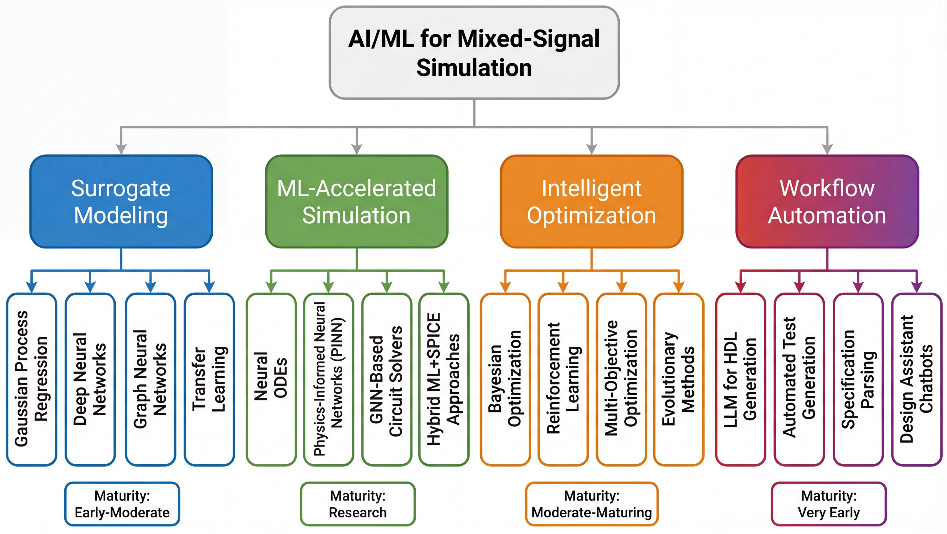
AI and ML methods for mixed-signal simulation have emerged as a significant research direction. Early work in the 1990s explored neural network device models with limited adoption. The modern revival began around 2017, driven by acute SPICE runtime bottlenecks, accumulated simulation datasets, growing parameter counts, and mature ML frameworks [24]. ML methods are complementary to SPICE, not replacements. Their value lies in accelerating design exploration, reducing expensive evaluations, and automating repetitive tasks. Figure 3 classifies these AI/ML methods by their role in the simulation workflow. This section evaluates their capabilities and limitations using the proposed framework.
4.1. Surrogate Models
Surrogate models approximate simulator input–output relationships, trained on SPICE results to predict performance without additional simulations.
Gaussian process regression (GPR) provides predictions with uncertainty quantification via a posterior variance [56], valuable for guiding sampling. Lyu et al. [21] demonstrated batch Bayesian optimization (BO) with GP surrogates for analog sizing, matching expert designers with reduced simulation budgets. He et al. [57] developed multi-fidelity GP models combining cheap approximate with expensive accurate simulations. Standard GPR’s complexity limits training sets to ∼1000–5000 points; sparse GP methods reduce this to [56]. Gu et al. [58] proposed BBGP-sDFO combining batch BO with subspace decomposition for high-dimensional synthesis.
Figure 3.
Classification of AI and machine learning methods applied to mixed-signal simulation, organized by their role in the simulation workflow: surrogate modeling for performance prediction, ML-accelerated solvers for direct simulation speedup, intelligent optimization for design space exploration, and LLM-based assistance for workflow automation.
Neural network surrogates scale to larger datasets than GPs. Budak et al. [20] demonstrated DNN surrogates with RL for analog sizing (10–50× speedup). CNNs have been applied to layout-aware prediction, and attention mechanisms identify influential parameters [59].
Graph neural networks (GNNs) naturally suit circuits as graph-structured objects (devices as nodes, interconnections as edges). Hakhamaneshi et al. [19] demonstrated pretraining and few-shot fine-tuning across topologies. Li et al. [59] achieved 3–5% prediction error with topology generalization. GNNs offer topology awareness: structural changes (e.g., adding a cascode) do not require complete retraining.
Transfer learning leverages source-domain knowledge (e.g., 28 nm) for target domains (e.g., 7 nm) with limited data [19,60]. Cross-technology transfer exploits qualitatively preserved circuit relationships. Sun et al. [61] demonstrated cross-technology migration via multi-agent RL with domain randomization.
Surrogates are useful for exploration (identifying promising regions, understanding trade-offs) but not for signoff. Typical accuracy of 5–15% [19,20] is insufficient where specifications have 1–2% margins, and accuracy degrades in underrepresented regions of the design space. It is worth noting that for fundamental analog circuits such as amplifiers and filters, parameter optimization is still largely conducted using classical optimization theories (gradient-based methods, geometric programming) with well-established convergence guarantees. Whether neural network-based surrogates can consistently outperform classical approaches for such parameter-tuning tasks—particularly when the cost of generating training data is considered—remains an open question that requires further systematic investigation.
4.2. ML-Accelerated Simulation
A more ambitious direction seeks to accelerate simulation itself by replacing solver components with learned models.
Neural ordinary differential equations (Neural ODEs) [62] learn circuit dynamics from SPICE waveforms, potentially enabling larger timesteps than traditional integrators. However, stability is not guaranteed outside training distributions, conservation laws (KCL, KVL) are not enforced, and training data requirements are substantial. These limitations restrict Neural ODEs to research demonstrations rather than production use.
Physics-informed neural networks (PINNs) embed physical laws (KCL, KVL, device equations) as training constraints [63]:
where penalizes deviation from training data and remaining terms penalize physics violations with weights . PINNs have been applied to parasitic extraction, thermal simulation, and IR drop analysis. They generalize better than pure data-driven models by preventing physically impossible predictions, but balancing loss terms remains challenging and convergence can be slow [63].
GNN-based circuit simulation via message-passing mimics iterative circuit solving, naturally capturing the graph structure of circuit networks. However, generalization to unseen topologies is limited and accuracy (1–10% vs. SPICE [59]) is acceptable only for exploration, not verification.
The most pragmatic hybrid approaches combine ML with SPICE rather than replacing it. ML-initialized SPICE reduces NR iterations using ML-predicted initial guesses. Adaptive fidelity screens with surrogates then applies SPICE to promising designs. ML-enhanced time stepping predicts appropriate step sizes based on learned waveform characteristics. These preserve SPICE as the accuracy arbiter while leveraging ML for efficiency. He et al. [57] demonstrated multi-fidelity approaches balancing speed and accuracy across simulation hierarchies.
Reported speedups of 10–1000× depend on complexity, tolerance, and whether training time is amortized. Training cost must be included in any fair comparison; typical accuracy is 1–10% in the training domain but degrades substantially for extrapolation. For exploration, 5% error suffices; for signoff, it does not.
4.3. Intelligent Optimization
Intelligent optimization is the most mature AI/ML application in mixed-signal design, addressing the expensive SPICE evaluation bottleneck at the core of analog circuit sizing.
Bayesian optimization (BO) maintains a GP surrogate and uses acquisition functions (Expected Improvement, Upper Confidence Bound, Knowledge Gradient) to balance exploration and exploitation [64]. BO identifies high-quality designs with 50–200 evaluations versus thousands for gradient-free methods [21]. Key extensions address scalability challenges: batch BO enables parallel evaluation of multiple designs per iteration [57,65]; constrained BO handles multiple specifications simultaneously via feasibility-aware acquisition functions [66]; and high-dimensional BO employs subspace decomposition techniques for circuits with 50+ design parameters, including tSS-BO [67] and D3PBO [68]. Gu et al. [58] proposed BBGP-sDFO combining batch BO with subspace derivative-free optimization. The MARIO framework [69] combines multiple optimization strategies for superadditive performance, and HiMOSS [70] advances gradient-based multi-objective optimization in high-dimensional spaces.
Reinforcement learning (RL) formulates sizing as sequential decision-making with deep algorithms (DQN, PPO, SAC) [71,72]. RL incorporates designer knowledge via reward shaping and can learn generalizable sizing policies. Multi-agent RL decomposes complex circuits across cooperative agents: Bao et al. [73] demonstrated MA-RL for complex analog design, Sun et al. [61] proposed EVDMARL for cross-technology migration with domain randomization, and Feng et al. [74] introduced hierarchical RL-optimization integration. However, RL requires thousands of evaluations per topology, limiting applicability to frequently redesigned circuits.
Multi-objective optimization seeks Pareto-optimal sets for conflicting specifications (e.g., gain vs. bandwidth vs. power). Approaches include NSGA-II and MOEA/D combined with surrogates. Zhao et al. [75] developed VTSMOC for constrained high-dimensional Pareto approximation, and APPLE-DSE [76] leverages asynchronous parallel computation. Evolutionary algorithms (genetic algorithms, PSO, differential evolution) handle global search and discrete variables [23]. AnalogGym [77] provides standardized benchmarks for fair comparison across methods. Topology optimization, explored by Shen et al. [78] (ATOM framework), addresses the harder problem of automatic circuit structure determination.
4.4. LLMs and Pragmatic Assessment
LLMs have demonstrated utility in HDL code generation (ChipChat [79], RTLCoder [80]), testbench generation, debugging, and tool orchestration (ChatEDA [22]). For mixed-signal design, LLM applications remain very limited—analog design requires continuous parameter optimization governed by physics, where LLMs have no inherent advantage. Shen et al. [81] proposed Atelier using LLM agents for qualitative tasks (specification interpretation, topology selection) with numerical optimization for sizing, acknowledging LLMs’ limitation to qualitative reasoning. Combining vision models (schematic understanding), language models (specification parsing), and numerical models (optimization) remains largely aspirational. LLMs assist EDA workflows (code generation, documentation, tool interfacing) but cannot perform direct circuit design—the gap between language understanding and circuit physics is fundamental. Recent work has demonstrated that LLMs can support structured technical tasks in resource-constrained environments beyond EDA, such as lightweight RF fingerprint identification for 6G edge intelligence [82], illustrating the broader potential of LLM-assisted engineering workflows.
4.4.1. What Truly Works Today
- BO for circuit sizing: most mature, available in commercial tools, with principled exploration–exploitation [21,58,66,67,68].
- Surrogates for exploration: useful for identifying promising design regions with SPICE validation before signoff.
- GNNs for prediction: promising for specific circuit families with topology awareness, though limited generalization.
- LLMs for workflow: genuine productivity gains in code generation, documentation, and tool interfacing.
4.4.2. What Remains Aspirational
Fully automated specification-to-layout design, end-to-end neural simulation replacing SPICE, LLM-driven analog design, and universal circuit foundation models [19] remain research aspirations. The pragmatic path is hybrid human–AI workflows: AI handles exploration and routine tasks while designers provide intuition, domain knowledge, and final verification.
4.4.3. Practical Deployment Considerations
Training ML models for circuit applications requires 200–5000 SPICE simulations depending on dimensionality [57]. For hour-long simulations, this means hundreds to thousands of CPU-hours before any benefit, making transfer learning and multi-fidelity methods essential for data efficiency. Designers need to understand why designs work, requiring trade-off explanations and margin analysis that black-box models cannot inherently provide. Models rarely transfer across topologies and technology nodes—a GP trained for a 28 nm op-amp has limited value for 7 nm GAA designs. ML can fail silently—returning plausible but incorrect predictions without diagnostics, unlike SPICE’s convergence warnings. Confident errors in underrepresented regions are the most serious industrial concern. Key deployment barriers include certification requirements for safety-critical applications (ISO 26262 [35]), reproducibility concerns from stochastic training, integration difficulty with existing tool chains, and justified designer skepticism of black-box predictions. The practical relevance of data-driven methods in electronic applications extends beyond circuit simulation to areas such as condition monitoring and predictive maintenance of power devices, where prediction and physical system behavior must be jointly considered [83].
5. Systematic Comparison and Analysis
This section synthesizes the preceding evaluations into a comparative framework, applying the proposed taxonomy and metrics to produce cross-cutting analysis.
5.1. Method Comparison
Table 3 applies the five-metric evaluation framework (Section 2.2) to compare thirteen method categories across the three taxonomy axes. Each row corresponds to a distinct region in the abstraction–solver–analysis classification space; the columns map directly to the five evaluation metrics. This structure enables practitioners to identify the most suitable method for a given design task by matching its taxonomy coordinates to the table entries.
Table 3.
Systematic comparison of mixed-signal simulation method categories. Accuracy is expressed relative to SPICE or silicon measurements. Speed indicates typical throughput relative to conventional SPICE. Capacity denotes the maximum practical circuit or system size. Maturity reflects years of development and industrial deployment status.
Key observations from the proposed framework: classical methods (SPICE, FastSPICE, RF/PSS) remain the only signoff-accurate approaches [9,10,29]; behavioral/system-level methods provide speedup at reduced fidelity [8,12,17]; MOR achieves high accuracy and speed for linear parasitic reduction [18]; and AI/ML spans a wide maturity range from production-ready BO [21,64] to early-stage LLMs [22].
5.2. AI/ML Method Comparison
Table 4 evaluates eight AI/ML techniques using the proposed framework. These methods primarily augment the solver-methodology axis by introducing data-driven alternatives to classical numerical solvers, with varying implications for accuracy, throughput, and convergence reliability.
Table 4.
Comparison of AI/ML methods applied to AMS simulation and design. Application refers to the primary use case in the AMS workflow. Maturity reflects the level of industrial validation and deployment.
Maturity stratifies clearly: GP/DNN are most mature (integrated in commercial tools [84,85]); GNN/RL are intermediate with promising but limited industrial validation [19,71]; Neural ODE, PINN, and LLM remain at research stage [22,62,63].
5.3. Industrial Tool Ecosystem
Table 5 maps the industrial EDA ecosystem onto the proposed taxonomy, showing how commercial tools implement the method categories classified in Table 3. Each tool occupies specific regions of the taxonomy space, and the table highlights how vendors differentiate along the five evaluation metrics. Three major vendors—Cadence, Synopsys, and Siemens EDA—dominate AMS simulation, competing on accuracy, speed, capacity, integration, and increasingly AI features.
Table 5.
Comparison of major commercial and open-source AMS simulation tools. Simulation type indicates primary engine category. Parallel indicates native multi-core or distributed support.
Cadence centers on Spectre [40] with APS/XPS acceleration tiers, AMS Designer [51] coupling Spectre with Xcelium for co-simulation, the Virtuoso ADE front-end, and Cerebrus [86] for RL-driven design optimization. Synopsys offers HSPICE as the industry signoff reference with first-day PDK support, CustomSim for FastSPICE capacity, VCS-AMS [52] for co-simulation, PrimeSim unifying multiple engines, and DSO.ai [85] for BO/RL-based optimization deployed in production at major companies. Siemens EDA provides ELDO with automotive reliability analysis (ISO 26262 compliance), Questa ADMS [53] for co-simulation, and Solido [84] using GP models and importance sampling for ML-accelerated variation-aware yield estimation.
Cadence Cerebrus [86] applies RL to optimize sizing within Virtuoso. Synopsys DSO.ai [85] combines BO and RL, deployed in production tapeouts. Siemens Solido [84] uses GP-based surrogates for ML-accelerated Monte Carlo. The overarching trend is embedding ML into existing tools rather than building replacements, augmenting designers while preserving SPICE for signoff.
A significant gap persists between open-source tools (ngspice [37], Xyce [36]) and commercial platforms in model support, verification infrastructure, and performance. Open-source tools provide essential research infrastructure and reproducible benchmarking, with AnalogGym [77] advancing standardized evaluation.
5.4. Cross-Cutting Analysis
Applying the proposed taxonomy reveals several cross-cutting findings. First, no single method dominates all phases: SystemC-AMS and RNM serve early exploration; Verilog-AMS enables block-level co-simulation; SPICE provides signoff accuracy; FastSPICE handles post-layout verification; MOR enables parasitic inclusion; and AI/ML augments at bottleneck points. A method’s value must be assessed within the complete design flow context.
Second, methods occupy distinct regions in the accuracy–speed–maturity landscape: SPICE (high accuracy, low speed, high maturity); FastSPICE/MOR (higher speed, maintained accuracy); behavioral/system-level (fast, lower accuracy); ML surrogates (fastest, moderate accuracy, low maturity). The path to AI adoption lies in augmenting mature tools, consistent with vendor strategies [84,85,86].
Third, the academic-to-industry gap is driven by three factors: foundry model support (academic work uses simplified models vs. industrial PDKs with hundreds of parameters), limited topology diversity in benchmarks (canonical op-amps vs. thousands of industrial topologies), and overfitting to specific circuits [19,77].
Table 6 provides a compact synthesis mapping main method families to their best-use scenarios and primary limitations, serving as a practical quick-reference for method selection.
Table 6.
Method family quick-reference: best-use scenario and main limitation for practical method selection guidance.
Fourth, four pragmatic insights emerge: (1) BO is the clear AI success story, with principled GP-based optimization integrated into all major vendor platforms [21,84,85,86]; (2) surrogates aid exploration, not signoff, as 5–15% error is insufficient for 1–2% margin specifications; (3) SPICE persists as the foundation, being augmented not replaced, due to its mathematical rigor and silicon-validated trust; and (4) ML’s greatest impact may be in verification efficiency—intelligent stimulus generation, coverage optimization, and ML-enhanced importance sampling—rather than simulation replacement.
6. Discussion
6.1. Implications of the Taxonomy Framework
The proposed three-axis taxonomy reveals systematic gaps in the method landscape. The (behavioral, ML-surrogate, statistical) region—where ML-enhanced behavioral models could accelerate Monte Carlo at the system level—is largely unexplored. Similarly, few methods address the (system-level, hybrid, noise) space, leaving system-level noise-aware simulation as an open challenge. The taxonomy provides practitioners with structured guidance for method selection: given a design task’s position in the classification space, the comparative tables (Table 3 and Table 4) identify applicable methods with their trade-offs. For instance, a post-layout verification task occupies (transistor, FastSPICE, transient) with clear tool choices, while an early-stage SoC exploration task maps to (system, co-simulation, transient) where SystemC-AMS or RNM are indicated. The framework also highlights that industrial tool selection is often constrained by vendor ecosystem lock-in rather than optimal method fit—an important practical consideration that purely technical comparisons miss.
6.2. Open Challenges
The transition to GAA nanosheets and CFET architectures introduces modeling challenges of unprecedented complexity [7,87]. At sub-3 nm, quantum effects (tunneling, confinement), self-heating in nanoscale fins, and growing process variability become first-order effects that compact models must capture with increasing parameter counts. Backside power delivery networks introduce 3D extraction and multi-physics challenges. Chiplet-based 3D integration [88] requires simulation across heterogeneous technology nodes with multi-physics coupling (electrical, thermal, mechanical)—an unsolved problem that existing single-domain simulators cannot address.
The AMS simulation capacity gap widens as SoCs grow to billions of transistors. Cloud computing [89,90] offers elastic scaling synergistic with AI-driven optimization but raises data security, latency, and cost concerns. Hierarchical approaches that automatically decompose systems, select per-block fidelity levels, and control inter-block error propagation remain incompletely solved. The energy cost of large-scale simulation is also an emerging sustainability concern.
ML’s silent failure mode—plausible but incorrect predictions without diagnostics—is the most fundamental AI trustworthiness challenge [24]. Uncertainty quantification via GP variance [56] or ensembles provides partial protection, but safety-critical standards (ISO 26262 [35]) require formal guarantees, explainability, and reproducibility that no current ML method satisfies simultaneously. Training data bias further undermines reliability in underrepresented corner cases. Progress requires certified uncertainty quantification, physics-informed constraints [63], and formal verification of ML properties.
Absent standardized benchmarks and protocols, cross-study comparison of AI methods is unreliable. Many studies use proprietary PDKs and tools, preventing replication. Adopting open design kits (SkyWater SKY130, GF180MCU), standardized protocols, public datasets, and community leaderboards would improve reproducibility [37,77]. ML tools must also integrate seamlessly with established workflows (Cadence Virtuoso, Synopsys Custom Compiler)—the “last mile” from research prototype to production tool remains acute.
6.3. Future Directions
Several directions appear most impactful for advancing the field. Digital twins for IC design would create continuously updated virtual replicas refined through fabrication, silicon measurement, and field data, enabling predictive maintenance and accelerated qualification via ML-based model calibration and data fusion. Foundation models for circuits would learn general circuit representations from large simulation corpora, pre-trained on diverse topologies and fine-tunable for specific tasks; early work includes GNN pretraining [19] and LLM assistants [22,81], but large-scale curated circuit datasets are prerequisites. Automated methodology selection systems would analyze netlists to recommend optimal simulation approaches per block and design phase, directly leveraging the taxonomy proposed in this paper to democratize access to advanced capabilities. Simulation–measurement convergence through Bayesian fusion of simulation predictions with silicon data would enable continuous model refinement, particularly valuable for analog IP reuse across technology nodes.
Priority roadmap. Based on our analysis, we propose a three-horizon research agenda:
- Short-term (1–3 years): Standardize open benchmarks and evaluation protocols for AI/ML methods in AMS design [77]; integrate Bayesian optimization into all major commercial tool flows; develop certified uncertainty quantification for ML surrogates.
- Medium-term (3–5 years): Achieve cross-technology transfer learning that generalizes across process nodes; develop automated methodology-selection systems leveraging the proposed taxonomy; create hybrid simulation engines combining SPICE accuracy with ML-accelerated exploration.
- Long-term (5–10 years): Realize digital twin frameworks for IC design with continuous model refinement from silicon data; develop foundation models for circuits pre-trained on large-scale simulation corpora; achieve simulation–measurement convergence through Bayesian data fusion.
6.4. Verification as a Cross-Cutting Concern
While this paper focuses on simulation methods, verification is an essential companion discipline. Formal methods (hybrid automata, reachability analysis [28]), runtime monitoring, and statistical verification provide complementary assurance. These techniques interact with the simulation methods classified here—formal methods may bound the regions where simulation must be accurate, while statistical verification determines how many simulations are needed for yield confidence. Integrating verification-aware metrics into the proposed framework is a direction for future work.
7. Conclusions
This paper has proposed a systematic taxonomy and comparative evaluation framework for mixed-signal simulation methods, addressing the absence of a unified classification system spanning the full spectrum from classical SPICE algorithms to contemporary AI-enhanced approaches. The three-axis taxonomy (abstraction level × solver methodology × analysis type) and five-metric evaluation framework provide a structured basis for comparing thirteen classical method categories and eight AI/ML approaches.
The comparative analysis yields several key findings. Classical simulation methods—SPICE, FastSPICE, and RF/PSS—remain the only approaches providing signoff-level accuracy and continue to serve as the foundational layer of AMS verification. Among AI/ML methods, Bayesian optimization for analog circuit sizing represents the most mature and industrially validated contribution, with demonstrated integration across all three major commercial EDA platforms. Surrogate models provide value for design exploration but lack the accuracy required for signoff. More ambitious approaches—Neural ODE solvers, physics-informed neural networks, and LLM-based design assistants—remain at the research stage with substantial gaps between demonstrated capabilities and industrial requirements.
The proposed taxonomy identifies specific under-explored regions in the method landscape and provides practitioners with structured guidance for simulation method selection based on design context. The persistent academic-to-industry gap, driven by foundry model complexity and limited benchmark diversity, suggests that community-level investments in standardized benchmarks, open datasets, and reproducible evaluation protocols are prerequisites for translating AI research advances into industrial practice. The pragmatic path forward is hybrid workflows that augment classical simulation with AI at specific bottleneck points, preserving the accuracy guarantees of physics-based methods while leveraging the efficiency of data-driven approaches.
Practical takeaways by reader group. For circuit designers, the taxonomy provides structured guidance for selecting simulation methods matched to each design phase, with the clear message that SPICE remains indispensable for signoff while Bayesian optimization offers the most mature AI augmentation for sizing tasks. For CAD/EDA researchers, the identified gaps in the taxonomy space—particularly ML-enhanced behavioral modeling for system-level Monte Carlo and system-level noise-aware simulation—represent high-impact research opportunities with clear industrial relevance. For AI-for-EDA researchers, the comparative analysis highlights that bridging the academic-to-industry gap requires working with realistic foundry models and diverse topologies, and that the most impactful near-term contributions lie in augmenting existing tools (uncertainty quantification, intelligent sampling, automated methodology selection) rather than replacing them.
Author Contributions
Conceptualization, J.Y. (Jian Yu) and L.J.; methodology, J.Y. (Jian Yu); formal analysis, J.Y. (Jian Yu) and H.Z.; writing—original draft preparation, J.Y. (Jian Yu) and H.Z.; writing—review and editing, J.Y. (Jiawen Yuan) and L.J.; visualization, H.Z.; supervision, J.Y. (Jian Yu); project administration, J.Y. (Jian Yu) All authors have read and agreed to the published version of the manuscript.
Funding
This research received no external funding.
Institutional Review Board Statement
Not applicable.
Informed Consent Statement
Not applicable.
Data Availability Statement
The comparative analysis in this study is based on published literature and vendor documentation. No new experimental data were generated.
Conflicts of Interest
The authors declare no conflicts of interest.
Abbreviations
The following abbreviations are used in this manuscript:
| AMS | Analog/Mixed-Signal |
| SPICE | Simulation Program with Integrated Circuit Emphasis |
| EDA | Electronic Design Automation |
| MNA | Modified Nodal Analysis |
| MOR | Model Order Reduction |
| ML | Machine Learning |
| DNN | Deep Neural Network |
| GNN | Graph Neural Network |
| BO | Bayesian Optimization |
| RL | Reinforcement Learning |
| LLM | Large Language Model |
| SoC | System-on-Chip |
| RNM | Real Number Modeling |
| PVT | Process, Voltage, Temperature |
References
- Razavi, B. Design of Analog CMOS Integrated Circuits, 2nd ed.; McGraw-Hill Education: New York, NY, USA, 2017. [Google Scholar]
- Alioto, M. Enabling the Internet of Things: From Integrated Circuits to Integrated Systems; Springer: Cham, Switzerland, 2017. [Google Scholar] [CrossRef] [Scilit]
- Hasch, J.; Topak, E.; Schnabel, R.; Zwick, T.; Weigel, R.; Waldschmidt, C. Millimeter-Wave Technology for Automotive Radar Sensors in the 77 GHz Frequency Band. IEEE Trans. Microw. Theory Tech. 2012, 60, 845–860. [Google Scholar] [CrossRef] [Scilit]
- Murmann, B. ADC Performance Survey 1997–2024. 2024. Available online: https://github.com/bmurmann/ADC-survey (accessed on 1 March 2025).
- WSTS. World Semiconductor Trade Statistics (WSTS) Semiconductor Market Forecast. World Semiconductor Trade Statistics. 2024. Available online: https://www.wsts.org/ (accessed on 1 March 2025).
- BSIM Group. BSIM-CMG Technical Manual; University of California: Berkeley, CA, USA, 2017; Available online: https://bsim.berkeley.edu/models/bsimcmg/ (accessed on 1 March 2025).
- Chauhan, Y.S.; Lu, D.; Sriramkumar, V.; Khandelwal, S.; Duarte, J.P.; Paydavosi, N.; Niknejad, A.; Hu, C. FinFET Modeling for IC Simulation and Design: Using the BSIM-CMG Standard Model; Academic Press: San Diego, CA, USA, 2015. [Google Scholar]
- Kundert, K.S.; Zinke, O. The Designer’s Guide to Verilog-AMS; Kluwer Academic Publishers: Boston, MA, USA, 2004. [Google Scholar]
- Pillage, L.T.; Rohrer, R.A.; Visweswariah, C. Electronic Circuit and System Simulation Methods; McGraw-Hill: New York, NY, USA, 1995. [Google Scholar]
- Nagel, L.W.; Pederson, D.O. SPICE (Simulation Program with Integrated Circuit Emphasis); Technical Report ERL-M382; Electronics Research Laboratory, University of California: Berkeley, CA, USA, 1973. [Google Scholar]
- Christen, E.; Bakalar, K. VHDL-AMS—A Hardware Description Language for Analog and Mixed-Signal Applications. IEEE Trans. Circuits Syst. II Analog Digit. Signal Process. 1999, 46, 1263–1272. [Google Scholar] [CrossRef] [Scilit]
- Muñoz, D.; Melikyan, V.; Markosyan, A. Accelerating Mixed-Signal Validation Using Real Number Models. In Proceedings of the IEEE International Conference on Electronics, Circuits, and Systems (ICECS); IEEE: New York City, NY, USA, 2018; pp. 657–660. [Google Scholar]
- Nagel, L.W. SPICE2: A Computer Program to Simulate Semiconductor Circuits; Technical Report ERL-M520; Electronics Research Laboratory, University of California: Berkeley, CA, USA, 1975. [Google Scholar]
- Vladimirescu, A. The SPICE Book; John Wiley & Sons: New York, NY, USA, 1994. [Google Scholar]
- Sui, Y.F.; Bhatt, D.; Bhattacharya, S.; Kao, S. A Unified Event/Level Sensitive Transistor Level Timing Simulator. In Proceedings of the IEEE/ACM International Conference on Computer-Aided Design (ICCAD); IEEE: New York City, NY, USA, 1998; pp. 280–284. [Google Scholar]
- IEEE Std 1800-2012; Standard for SystemVerilog—Unified Hardware Design, Specification, and Verification Language. IEEE: New York City, NY, USA, 2013; Includes provisions for analog and mixed-signal extensions.
- Barnasconi, M.; Einwich, K.; Grimm, C.; Maehne, T.; Vachoux, A. SystemC-AMS: System-Level Modeling of Heterogeneous Systems. IEEE Des. Test Comput. 2012, 29, 78–88. [Google Scholar]
- Odabasioglu, A.; Celik, M.; Pileggi, L.T. PRIMA: Passive Reduced-Order Interconnect Macromodeling Algorithm. IEEE Trans. Comput.-Aided Des. Integr. Circuits Syst. 1998, 17, 645–654. [Google Scholar] [CrossRef] [Scilit]
- Hakhamaneshi, K.; Nassar, M.; Phielipp, M.; Abbeel, P.; Stojanovic, V. Pretraining Graph Neural Networks for Few-Shot Analog Circuit Modeling and Design. IEEE Trans. Comput.-Aided Des. Integr. Circuits Syst. 2023, 42, 2163–2176. [Google Scholar] [CrossRef] [Scilit]
- Budak, A.F.; Bhansali, P.; Liu, S.; Sun, N.; Pan, D.Z.; Kashyap, C.V. DNN-Opt: An RL Inspired Optimization for Analog Circuit Sizing Using Deep Neural Networks. In Proceedings of the 58th ACM/IEEE Design Automation Conference (DAC), San Francisco, CA, USA, 5–9 December 2021; pp. 1219–1224. [Google Scholar] [CrossRef] [Scilit]
- Lyu, W.; Yang, F.; Yan, C.; Zhou, D.; Zeng, X. Batch Bayesian Optimization via Multi-Objective Acquisition Ensemble for Automated Analog Circuit Design. In Proceedings of the 35th International Conference on Machine Learning (ICML), Stockholm, Sweden, 10–15 July 2018; pp. 3306–3314. [Google Scholar]
- Wu, H.; He, Z.; Zhang, X.; Yao, X.; Zheng, S.; Zheng, H.; Yu, B. ChatEDA: A Large Language Model Powered Autonomous Agent for EDA. IEEE Trans. Comput.-Aided Des. Integr. Circuits Syst. 2024, 43, 3583–3596. [Google Scholar] [CrossRef] [Scilit]
- Gielen, G.G.E.; Rutenbar, R.A. Computer-Aided Design of Analog and Mixed-Signal Integrated Circuits. Proc. IEEE 2000, 88, 1825–1852. [Google Scholar] [CrossRef] [Scilit]
- Huang, G.; Hu, J.; He, Y.; Liu, J.; Ma, M.; Shen, Z.; Wu, J.; Xu, Y.; Zhang, H.; Zhong, K.; et al. Machine Learning for Electronic Design Automation: A Survey. ACM Trans. Des. Autom. Electron. Syst. 2021, 26, 1–46. [Google Scholar] [CrossRef] [Scilit]
- Gildenblat, G.; Li, X.; Wu, W.; Wang, H.; Jha, A.; van Langevelde, R.; Smit, G.D.J.; Scholten, A.J.; Klaassen, D.B.M. PSP: An Advanced Surface-Potential-Based MOSFET Model for Circuit Simulation. IEEE Trans. Electron Devices 2006, 53, 1979–1993. [Google Scholar] [CrossRef] [Scilit]
- Rabaey, J.M.; Chandrakasan, A.; Nikolić, B. Digital Integrated Circuits: A Design Perspective, 2nd ed.; Prentice Hall: Upper Saddle River, NJ, USA, 2003. [Google Scholar]
- IEEE. IEEE Standard VHDL Analog and Mixed-Signal Extensions (IEEE Std 1076.1-2007). Defines Continuous-Time and Frequency-Domain Extensions to VHDL. 2007. Available online: https://ieeexplore.ieee.org/document/4384309 (accessed on 1 March 2025).
- Zaki, M.H.; Tahar, S.; Bois, G. Formal Verification of Analog and Mixed-Signal Designs: A Survey. Microelectron. J. 2008, 39, 1395–1404. [Google Scholar] [CrossRef] [Scilit]
- Kundert, K.S. Introduction to RF Simulation and Its Application. IEEE J. Solid State Circuits 1999, 34, 1298–1319. [Google Scholar] [CrossRef] [Scilit]
- Singhee, A.; Rutenbar, R.A. Extreme Statistics in Nanoscale Memory Design; Springer: New York, NY, USA, 2010. [Google Scholar] [CrossRef] [Scilit]
- Ho, C.W.; Ruehli, A.E.; Brennan, P.A. The Modified Nodal Approach to Network Analysis. IEEE Trans. Circuits Syst. 1975, 22, 504–509. [Google Scholar] [CrossRef] [Scilit]
- Quarteroni, A.; Sacco, R.; Saleri, F. Numerical Mathematics, 2nd ed.; Springer: Berlin, Germany, 2007. [Google Scholar] [CrossRef] [Scilit]
- Gear, C.W. Numerical Initial Value Problems in Ordinary Differential Equations; Prentice-Hall: Englewood Cliffs, NJ, USA, 1971. [Google Scholar]
- Xi, X.; Dunga, M.; He, J.; Liu, W.; Cao, K.M.; Jin, X.; Ou, J.J.; Chan, M.; Niknejad, A.M.; Hu, C. BSIM4.3.0 MOSFET Model—User’s Manual; Technical Report; Department of Electrical Engineering and Computer Sciences, University of California: Berkeley, CA, USA, 2004; Available online: https://bsim.berkeley.edu/models/bsim4/ (accessed on 1 March 2025).
- ISO 26262; Road Vehicles–Functional Safety, 2nd Edition. International Organization for Standardization: Geneva, Switzerland, 2018.
- Keiter, E.R.; Aadithya, K.V.; Mei, T.; Russo, T.V.; Schiek, R.L.; Sholander, P.E.; Thornquist, H.K.; Verley, J.C. Xyce Parallel Electronic Simulator: Reference Guide. Technical Report SAND2023-01032. Sandia National Laboratories. 2023. Available online: https://xyce.sandia.gov/ (accessed on 1 March 2025).
- Nenzi, P.; Vogt, H. Ngspice–Open Source Mixed-Mode, Mixed-Level Circuit Simulator. 2024. Available online: https://ngspice.sourceforge.io/ (accessed on 1 March 2025).
- Rizzoli, V.; Mastri, F.; Cecchetti, C.; Lipparini, A. General-Purpose Harmonic Balance Analysis of Nonlinear Microwave Circuits Under Multitone Excitation. IEEE Trans. Microw. Theory Tech. 1988, 36, 1650–1660. [Google Scholar] [CrossRef]
- Aprille, T.J.; Trick, T.N. Steady-State Analysis of Nonlinear Circuits with Periodic Inputs. Proc. IEEE 1972, 60, 108–114. [Google Scholar] [CrossRef] [Scilit]
- Cadence Design Systems, Inc. Spectre Simulation Platform; Cadence Design Systems, Inc.: San Jose, CA, USA, 2023. [Google Scholar]
- Brambilla, A.; Maffezzoni, P. Envelope-Following Method for the Transient Analysis of Electrical Circuits. IEEE Trans. Circuits Syst. I Fundam. Theory Appl. 2000, 47, 999–1008. [Google Scholar] [CrossRef] [Scilit]
- Pelgrom, M.J.M.; Duinmaijer, A.C.J.; Welbers, A.P.G. Matching Properties of MOS Transistors. IEEE J. Solid State Circuits 1989, 24, 1433–1440. [Google Scholar] [CrossRef] [Scilit]
- Kanj, R.; Joshi, R.; Nassif, S. Statistical Yield Estimation and Design of SRAM Cells. IEEE Des. Test Comput. 2006, 23, 493–504. [Google Scholar]
- McKay, M.D.; Beckman, R.J.; Conover, W.J. A Comparison of Three Methods for Selecting Values of Input Variables in the Analysis of Output from a Computer Code. Technometrics 1979, 21, 239–245. [Google Scholar] [CrossRef] [Scilit]
- Niederreiter, H. Random Number Generation and Quasi-Monte Carlo Methods; SIAM: Philadelphia, PA, USA, 1992. [Google Scholar] [CrossRef] [Scilit]
- Kundert, K.S. Challenges in Mixed-Signal Verification. In Proceedings of the IEEE Custom Integrated Circuits Conference (CICC); IEEE: New York City, NY, USA, 2005; pp. 367–374. [Google Scholar]
- Einwich, K.; Grimm, C.; Vachoux, A. SystemC AMS Extensions: Solving the Need for Speed. In Proceedings of the Design, Automation and Test in Europe Conference (DATE); IEEE: New York City, NY, USA, 2011; pp. 1–6. [Google Scholar]
- Kuhn, M.; Becker, B. Mixed-Signal Methodologies for SoC Verification Using Real Number Models. In Proceedings of the Design, Automation and Test in Europe Conference (DATE); IEEE: New York City, NY, USA, 2015; pp. 1574–1579. [Google Scholar]
- Sommer, R.; Kupferschmid, C.; Enge-Rosenblatt, O. Synchronization of Mixed-Signal Simulators. AEU–Int. J. Electron. Commun. 2008, 62, 161–167. [Google Scholar]
- Saleh, R.A.; Antognetti, P. Relaxation-Based Simulation of Mixed-Signal Circuits. In Proceedings of the IEEE/ACM International Conference on Computer-Aided Design (ICCAD); IEEE: New York City, NY, USA, 1990; pp. 486–489. [Google Scholar]
- Cadence Design Systems, Inc. AMS Designer User Guide; Cadence Design Systems, Inc.: San Jose, CA, USA, 2023. [Google Scholar]
- Synopsys, Inc. VCS AMS User Guide; Synopsys, Inc.: Mountain View, CA, USA, 2023. [Google Scholar]
- Siemens EDA. Questa ADMS User Manual; Siemens Digital Industries Software: Wilsonville, OR, USA, 2023. [Google Scholar]
- Antoulas, A.C. Approximation of Large-Scale Dynamical Systems; SIAM: Philadelphia, PA, USA, 2005. [Google Scholar] [CrossRef] [Scilit]
- Freund, R.W. Model Reduction Methods Based on Krylov Subspaces. Acta Numer. 2003, 12, 267–319. [Google Scholar] [CrossRef] [Scilit]
- Rasmussen, C.E.; Williams, C.K.I. Gaussian Processes for Machine Learning; MIT Press: Cambridge, MA, USA, 2006. [Google Scholar]
- He, B.; Zhang, S.; Wang, Y.; Gao, T.; Yang, F.; Yan, C.; Zhou, D.; Bi, Z.; Zeng, X. A Batched Bayesian Optimization Approach for Analog Circuit Synthesis via Multi-Fidelity Modeling. IEEE Trans. Comput.-Aided Des. Integr. Circuits Syst. 2023, 42, 347–360. [Google Scholar] [CrossRef] [Scilit]
- Gu, T.; Li, W.; Zhao, A.; Bi, Z.; Li, X.; Yang, F.; Yan, C.; Hu, W.; Zhou, D.; Cui, T.; et al. BBGP-sDFO: Batch Bayesian and Gaussian Process Enhanced Subspace Derivative Free Optimization for High-Dimensional Analog Circuit Synthesis. IEEE Trans. Comput.-Aided Des. Integr. Circuits Syst. 2024, 43, 1126–1139. [Google Scholar] [CrossRef] [Scilit]
- Li, Y.; Lin, Y.; Madhusudan, M.; Sharma, A.; Xu, W.; Sapatnekar, S.S.; Harjani, R.; Hu, J. A Graph Neural Network Framework for Circuit Performance Prediction. In Proceedings of the 59th ACM/IEEE Design Automation Conference (DAC); IEEE: New York City, NY, USA, 2022; pp. 1–6. [Google Scholar]
- Qian, L.; Bi, Z.; Zhou, D.; Zeng, X. Automated Technology Migration Methodology for Mixed-Signal Circuit Based on Multistart Optimization Framework. IEEE Trans. Very Large Scale Integr. (VLSI) Syst. 2015, 23, 2595–2605. [Google Scholar] [CrossRef] [Scilit]
- Sun, H.; Bi, Z.; Jiang, W.; Lu, Y.; Yan, C.; Yang, F.; Hu, W.; Wang, S.G.; Zhou, D.; Zeng, X. EVDMARL: Efficient Value Decomposition-based Multi-Agent Reinforcement Learning with Domain-Randomization for Complex Analog Circuit Design Migration. In Proceedings of the 61st ACM/IEEE Design Automation Conference (DAC); IEEE: New York City, NY, USA, 2024; pp. 1–6. [Google Scholar] [CrossRef] [Scilit]
- Chen, R.T.Q.; Rubanova, Y.; Bettencourt, J.; Duvenaud, D. Neural Ordinary Differential Equations. Proc. Adv. Neural Inf. Process. Syst. (NeurIPS) 2018, 31, 6571–6583. [Google Scholar] [CrossRef] [Scilit]
- Raissi, M.; Perdikaris, P.; Karniadakis, G.E. Physics-Informed Neural Networks: A Deep Learning Framework for Solving Forward and Inverse Problems Involving Nonlinear Partial Differential Equations. J. Comput. Phys. 2019, 378, 686–707. [Google Scholar] [CrossRef] [Scilit]
- Shahriari, B.; Swersky, K.; Wang, Z.; Adams, R.P.; de Freitas, N. Taking the Human Out of the Loop: A Review of Bayesian Optimization. Proc. IEEE 2016, 104, 148–175. [Google Scholar] [CrossRef] [Scilit]
- Zhao, X.; Bi, Z.; Yan, C.; Yang, F.; Lu, Y.; Zhou, D.; Zeng, X. Asynchronous Batch Constrained Multi-Objective Bayesian Optimization for Analog Circuit Sizing. In Proceedings of the 29th Asia and South Pacific Design Automation Conference (ASP-DAC), Incheon, Republic of Korea, 22–25 January 2024; pp. 1–6. [Google Scholar] [CrossRef] [Scilit]
- Zhao, A.; Wang, X.; Lin, Z.; Bi, Z.; Li, X.; Yan, C.; Yang, F.; Shang, L.; Zhou, D.; Zeng, X. cVTS: A Constrained Voronoi Tree Search Method for High Dimensional Analog Circuit Synthesis. In Proceedings of the 60th ACM/IEEE Design Automation Conference (DAC), San Francisco, CA, USA, 9–13 July 2023; pp. 1–6. [Google Scholar] [CrossRef] [Scilit]
- Gu, T.; Wang, J.; Bi, Z.; Yan, C.; Yang, F.; Qin, Y.; Cui, T.; Zeng, X. tSS-BO: Scalable Bayesian Optimization for Analog Circuit Sizing via Truncated Subspace Sampling. In Proceedings of the Design, Automation and Test in Europe Conference (DATE), Valencia, Spain, 25–27 March 2024; pp. 1–6. [Google Scholar] [CrossRef] [Scilit]
- Zhao, A.; Gu, T.; Bi, Z.; Yang, F.; Yan, C.; Zeng, X.; Lin, Z.; Hu, W.; Zhou, D. D3PBO: Dynamic Domain Decomposition based Parallel Bayesian Optimization for Large-scale Analog Circuit Sizing. ACM Trans. Des. Autom. Electron. Syst. 2024, 29, 1–25. [Google Scholar] [CrossRef] [Scilit]
- Li, W.; Meng, Y.; Lyu, R.; Yan, C.; Zhu, K.; Bi, Z.; Zhou, D.; Zeng, X. MARIO: A Superadditive Multi-Algorithm Interworking Optimization Framework for Analog Circuit Sizing. In Proceedings of the 62nd ACM/IEEE Design Automation Conference (DAC), San Francisco, CA, USA, 22–25 June 2025; pp. 1–7. [Google Scholar] [CrossRef] [Scilit]
- Gu, T.; Lyu, R.; Bi, Z.; Yan, C.; Yang, F.; Zhou, D.; Cui, T.; Liu, X.; Zhang, Z.; Zeng, X. HiMOSS: A Novel High-Dimensional Multi-Objective Optimization Method via Adaptive Gradient-Based Subspace Sampling for Analog Circuit Sizing. In Proceedings of the 61st ACM/IEEE Design Automation Conference (DAC), San Francisco, CA, USA, 23–27 June 2024; pp. 1–6. [Google Scholar] [CrossRef] [Scilit]
- Wang, H.; Wang, K.; Yang, J.; Shen, L.; Sun, N.; Lee, H.S.; Han, S. GCN-RL Circuit Designer: Transferable Transistor Sizing with Graph Neural Networks and Reinforcement Learning. In Proceedings of the 57th ACM/IEEE Design Automation Conference (DAC), San Francisco, CA, USA, 20–24 July 2020; pp. 1–6. [Google Scholar] [CrossRef] [Scilit]
- Settaluri, K.; Haj-Ali, A.; Huang, Q.; Hakhamaneshi, K.; Nikolic, B. AutoCkt: Deep Reinforcement Learning of Analog Circuit Designs. In Proceedings of the Design, Automation and Test in Europe Conference (DATE), Grenoble, France, 9–13 March 2020; pp. 490–495. [Google Scholar] [CrossRef] [Scilit]
- Bao, J.; Zhang, J.; Huang, Z.; Feng, X.; Bi, Z.; Zeng, X.; Lu, Y. Multiagent Based Reinforcement Learning (MA-RL): An Automated Designer for Complex Analog Circuits. IEEE Trans. Comput.-Aided Des. Integr. Circuits Syst. 2024, 43, 1437–1450. [Google Scholar] [CrossRef] [Scilit]
- Feng, X.; Xu, Y.; Huang, Z.; Xu, W.; Bi, Z.; Yang, F.; Zeng, X.; Lu, Y. Hierarchical Integration of Reinforcement Learning and Optimization Algorithms for Time-Efficient Design Automation of Complex Analog Circuit. ACM Trans. Des. Autom. Electron. Syst. 2025, 30, 1–22. [Google Scholar] [CrossRef] [Scilit]
- Zhao, A.; Lyu, R.; Zhao, X.; Bi, Z.; Yang, F.; Yan, C.; Zhou, D.; Su, Y.; Zeng, X. VTSMOC: An Efficient Voronoi Tree Search Boosted Multi-objective Bayesian Optimization with Constraints for High-dimensional Analog Circuit Synthesis. IEEE Trans. Comput.-Aided Des. Integr. Circuits Syst. 2024, 43, 4297–4310. [Google Scholar] [CrossRef] [Scilit]
- Zhao, X.; Gao, T.; Wu, Z.; Bi, Z.; Yan, C.; Yang, F.; Wang, S.G.; Zhou, D.; Zeng, X. APPLE-DSE: Asynchronous Parallel Pareto Set Learning for Microarchitecture Design Space Exploration. IEEE Trans. Comput.-Aided Des. Integr. Circuits Syst. 2024, 43, 3841–3854. [Google Scholar] [CrossRef] [Scilit]
- Li, J.; Zhi, H.; Lyu, R.; Li, W.; Bi, Z.; Zhu, K.; Zeng, Y.; Shan, W.; Yan, C.; Yang, F.; et al. AnalogGym: An Open and Practical Testing Suite for Analog Circuit Synthesis. In Proceedings of the 43rd IEEE/ACM International Conference on Computer-Aided Design (ICCAD), New York, NY, USA, 27–31 October 2024; pp. 1–9. [Google Scholar] [CrossRef] [Scilit]
- Shen, J.; Yang, F.; Shang, L.; Yan, C.; Bi, Z.; Zhou, D.; Zeng, X. ATOM: An Automatic Topology Synthesis Framework for Operational Amplifiers. IEEE Trans. Comput.-Aided Des. Integr. Circuits Syst. 2024, 43, 2092–2105. [Google Scholar] [CrossRef] [Scilit]
- Blocklove, J.; Garg, S.; Karri, R.; Pearce, H. Chip-Chat: Challenges and Opportunities in Conversational Hardware Design. In Proceedings of the 5th ACM/IEEE Workshop on Machine Learning for CAD (MLCAD), Snowbird, UT, USA, 10–13 September 2023; pp. 1–6. [Google Scholar] [CrossRef] [Scilit]
- Liu, S.; Fang, W.; Lu, Y.; Wang, J.; Zhang, Q.; Zhang, H.; Xie, Z. RTLCoder: Fully Open-Source and Efficient LLM-Assisted RTL Code Generation Technique. IEEE Trans. Comput.-Aided Des. Integr. Circuits Syst. 2024, 43, 3981–3993. [Google Scholar] [CrossRef] [Scilit]
- Shen, J.; Chen, Z.; Zhuang, J.; Huang, J.; Yang, F.; Shang, L.; Bi, Z.; Yan, C.; Zhou, D.; Zeng, X. Atelier: An Automated Analog Circuit Design Framework via Multiple Large Language Model-based Agents. IEEE Trans. Comput.-Aided Des. Integr. Circuits Syst. 2025, 45, 31–44. [Google Scholar] [CrossRef] [Scilit]
- Gao, N.; Liu, Y.; Zhang, Q.; Li, X.; Jin, S. Let RFF do the talking: Large language model enabled lightweight RFFI for 6G edge intelligence. Sci. China Inf. Sci. 2025, 68, 170308. [Google Scholar] [CrossRef] [Scilit]
- Wei, J.; Liang, F.; Feng, H.; Ran, L. Condition Monitoring of Discrete Power Devices: A Data-Driven Approach with Stress Quantification and Mold Temperature Sensing. IEEE J. Emerg. Sel. Top. Power Electron. 2024, 12, 2569–2579. [Google Scholar] [CrossRef] [Scilit]
- Siemens EDA. Siemens Solido Design Environment. Product Documentation. ML-Based Variation-Aware Design and Characterization. 2024. Available online: https://eda.sw.siemens.com/en-US/ic/solido/ (accessed on 1 March 2025).
- Synopsys, Inc. Synopsys DSO.ai–Autonomous Chip Design. Product Documentation. AI-Driven Design Space Optimization. 2024. Available online: https://www.synopsys.com/ai/ai-powered-eda/dso-ai.html (accessed on 1 March 2025).
- Cadence Design Systems, Inc. Cadence Cerebrus Intelligent Chip Explorer. Product Documentation. AI-Driven Design Optimization Platform. 2024. Available online: https://www.cadence.com/en_US/home/tools/digital-design-and-signoff/soc-implementation-and-floorplanning/cerebrus-intelligent-chip-explorer.html (accessed on 1 March 2025).
- Barraud, S.; Previtali, B.; Vizioz, C.; Hartmann, J.M.; Sturm, J.; Widiez, J.; Vinet, M. Performance and Design Considerations for Gate-All-Around Stacked-Nanowires FETs. In Proceedings of the 2017 IEEE International Electron Devices Meeting (IEDM), San Francisco, CA, USA, 2–6 December 2017; pp. 29.2.1–29.2.4. [Google Scholar] [CrossRef] [Scilit]
- Stow, D.; Akgun, I.; Fan, Y.; Mulay, G.; Xie, Y. Cost and Thermal Analysis of High-Performance Chiplet-Based Multi-Chip Modules. In Proceedings of the IEEE Computer Society Annual Symposium on VLSI (ISVLSI), San Jose, CA, USA, 11–13 July 2017; pp. 233–240. [Google Scholar]
- Cadence Design Systems, Inc. Cadence CloudBurst Platform for Hybrid Cloud. Product Documentation. Cloud-Native EDA Platform. 2024. Available online: https://www.cadence.com/en_US/home/solutions/cadence-cloud.html (accessed on 1 June 2025).
- Synopsys, Inc. Synopsys Cloud. Product Documentation. Cloud-Based EDA Solution. 2024. Available online: https://www.synopsys.com/cloud.html (accessed on 1 June 2025).
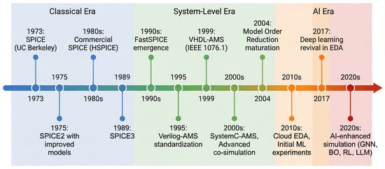
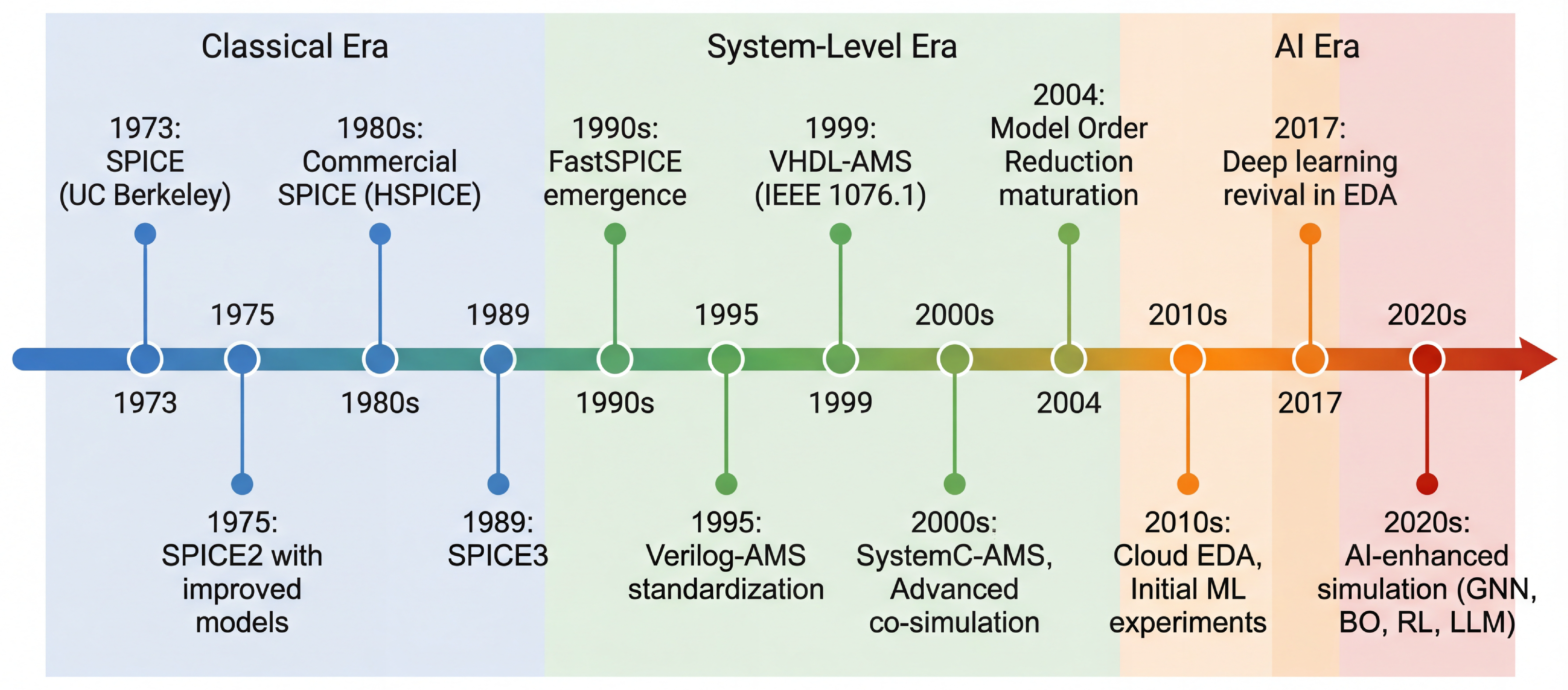
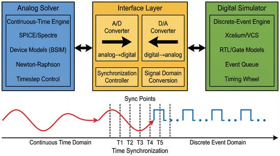
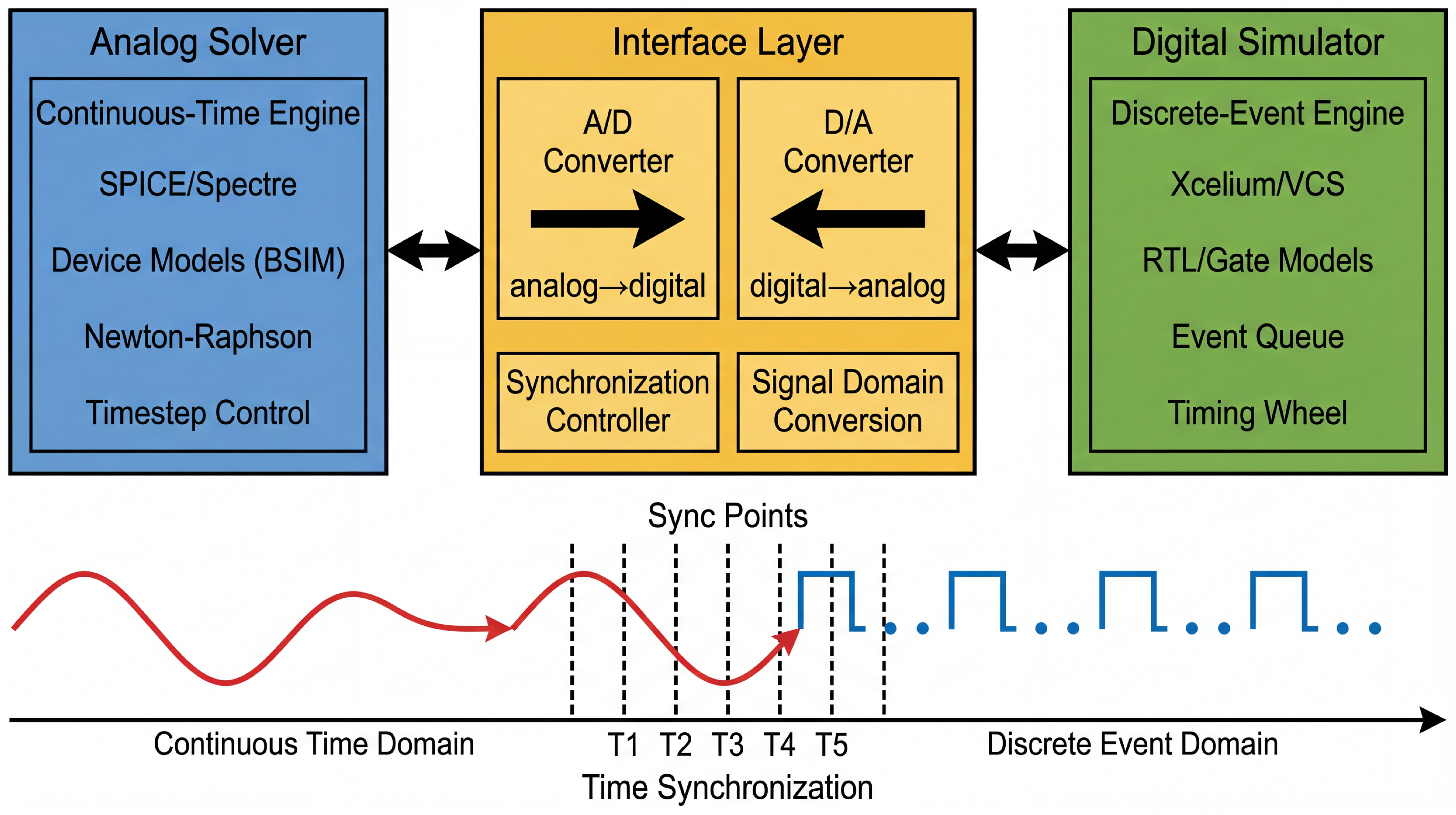

Disclaimer/Publisher’s Note: The statements, opinions and data contained in all publications are solely those of the individual author(s) and contributor(s) and not of MDPI and/or the editor(s). MDPI and/or the editor(s) disclaim responsibility for any injury to people or property resulting from any ideas, methods, instructions or products referred to in the content. |
© 2026 by the authors. Licensee MDPI, Basel, Switzerland. This article is an open access article distributed under the terms and conditions of the Creative Commons Attribution (CC BY) license.