Analysis of Energy Efficiency in Green Cluster Computing

Abstract

Energy efficiency in computing has emerged as a critical concern due to escalating environmental and financial costs, particularly in the context of cluster computing, where there is an ever-increasing software workload. Achieving meaningful improvements in energy efficiency requires a comprehensive understanding of the interplay between hardware and software. This research investigates how algorithmic optimisations, language choice, and parallelisation strategies influence energy efficiency and how hardware-level strategies such as underclocking, overclocking, cooling, and on-demand computing can further impact energy usage. A set of measures that can be used generally to show the impact trade-off of power and performance are defined, including the Energy Factor (EF) and a new Efficiency–Performance Score (EPS). Validation experiments on a custom-built Raspberry Pi Bramble cluster used workloads like Monte Carlo Pi simulations in Python and C. Energy and performance trade-offs were evaluated using the Energy Factor and Efficiency–Performance Score on a small example cluster to validate the approach. Results show parallelisation greatly improves energy efficiency over serial execution. Cooling slightly boosts speed under heavy loads but increases total energy use. Perhaps counter-intuitively, underclocking actually raises total energy consumption, while overclocking reduces it. Language choice also impacts efficiency, with C offering notable energy savings over Python. The findings support the hypothesis that software optimisation alone can improve energy efficiency, but the most impactful results are achieved when both software and hardware strategies are jointly considered. These insights contribute to the design of future energy-aware computing systems and provide a foundation for sustainable, high-performance computing architectures.

1. Introduction

The rising environmental and financial costs of large-scale computing [1] necessitate energy-efficient system design. This research investigates how hardware and software optimisations affect energy efficiency in cluster computing. The goal is to demonstrate that integrating energy-aware strategies at both levels can enhance performance while reducing energy consumption.

Higher-level languages offer improved usability; however, they often introduce resource overhead compared to lower-level languages [2]. Similarly, the performance gains obtained through parallelisation may improve energy efficiency by reducing execution time but can also increase total energy consumption if additional power draw is not offset. Additionally, algorithmic improvements in software design can enhance energy efficiency. For instance, reducing the complexity of a program from $O\left(n^3\right)$ to a lower order reduces unnecessary computation, thereby conserving energy [3].

From a hardware perspective, strategies such as cooling, clock-speed adjustment, and alternative hardware architectures may contribute to energy savings [4]. Cooling components like the CPU and GPU help prevent thermal throttling, thereby maintaining higher performance and utilisation. However, this can also lead to increased overall energy consumption, as the system operates more efficiently and performs more computations per second, unlike throttled components, which consume less energy as a consequence of reduced computational activity. Adjusting the clock speed of computing components directly affects the rate at which computations are performed. While increasing the clock speed typically leads to higher power draw, it can also reduce overall energy consumption if the performance gain significantly shortens execution time. Conversely, underclocking may lower power draw but prolong computation, potentially increasing the total energy consumed. Additionally, as novel computing paradigms continue to evolve, system architectures may increasingly shift away from traditional models toward designs that prioritise energy efficiency, such as heterogeneous systems or domain-specific accelerators.

This study introduces a generalizable set of measurement approaches and metrics that can be used to show the trade-off between power usage and system performance and bridge the gap between software optimisations and hardware configurations—areas often studied separately. A validation experiment was performed to show how these measurements can be used on a custom Raspberry Pi cluster, demonstrating how energy consumption differs depending on the choice of language, the efficiency of the algorithm, parallelisation strategies and implementations, cooling, underclocking, overclocking, and on-demand computing.

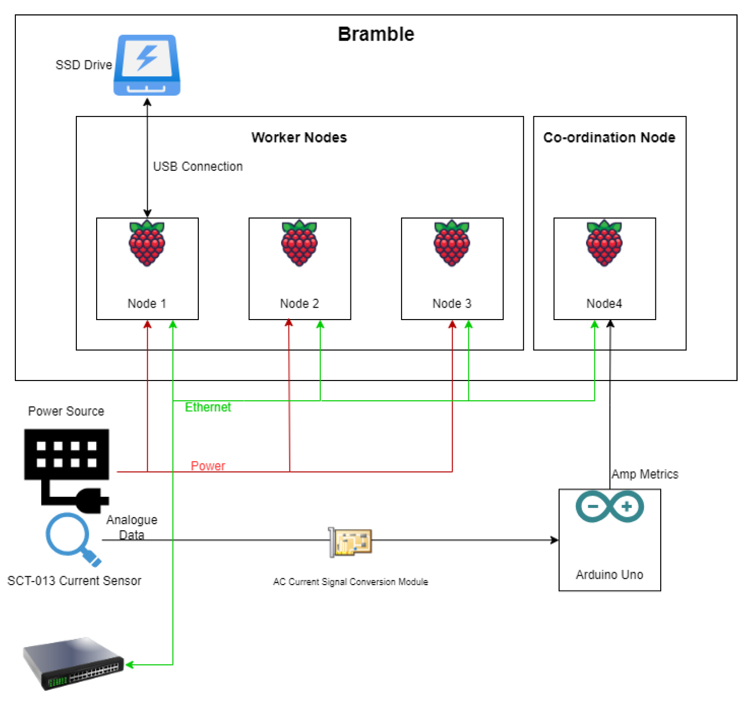
The setup consists of three Raspberry Pis running Raspbian Lite, networked via a switch and monitored by an Arduino Uno with an SCT-013 current sensor. A fourth Pi acts as coordinator and energy logger, with workloads (e.g., Monte Carlo Pi) executed using MPI and OMP in Python and C to evaluate energy efficiency.

To calculate continuous energy (the running draw of energy), the following equation can be applied:

$$Watts=Amps\times Voltage$$

(1)

To calculate the total energy consumption of a software workload, continuous power readings are taken throughout its execution. Since power consumption can fluctuate based on workload intensity, a weighted average of these readings is computed, then multiplied by the total runtime to estimate energy usage. In this study, workloads varied from a few seconds to several minutes in duration, with some extending to over an hour. As such, energy is expressed in Watt hours (Wh):

$$Watt\text{–}Hour \left(\mathrm{Wh}\right)=Watts\times Hours$$

(2)

To evaluate the impact of different strategies on energy consumption, it is first essential to define what is meant by energy efficiency in this context. Here, energy efficiency refers to the ability to complete a fixed set of computations while limiting the total amount of energy used.

This notion of efficiency can be formalised using the metric of the Energy Factor ($EF$), which quantifies the relative change in energy consumption when applying a new strategy compared to a baseline. An $EF$ greater than 1 indicates improved efficiency, whereas an $EF$ less than 1 implies greater energy use for the same output.

$$EF\left(EnergyFactor\right)={\displaystyle \frac{InitialEnergyRequirements}{NewEnergyRequirements}}$$

(3)

To complement this, Speedup is used to measure the improvement in execution time:

$$\mathrm{Speedup}={\displaystyle \frac{\mathrm{Previous}\mathrm{Time}\mathrm{Taken}}{\mathrm{New}\mathrm{Time}\mathrm{Taken}}}$$

(4)

Again, a value above 1 indicates a faster execution, while a value below 1 indicates a slowdown. In both metrics, the desired outcome is for the new configuration to use less time or energy, resulting in a score greater than 1.

A simple combined metric could be a direct division of $EF$ and Speedup:

$$EP{S}_{\mathrm{simple}}={\displaystyle \frac{EF}{Speedup}}$$

(5)

However, this approach may be overly influenced by extreme values in either energy or performance. To address this, a geometric mean is used—a simple approach to reduce the impact of extreme outliers as seen in real-world experimentation, resulting in a more balanced metric called the Efficiency–Performance Score ($EPS$):

$$EPS=\sqrt{EF\times Speedup}$$

(6)

This formulation ensures that both energy efficiency and performance contribute equally to the final score, preventing one from disproportionately dominating the result.

It is anticipated that results will highlight the interdependency of software and hardware optimisations, revealing that neither approach alone can fully address energy inefficiency. Instead, a combined strategy is expected to yield significant reductions in energy consumption without compromising performance. Moreover, applying both software optimisations (e.g., parallelisation and algorithmic refinement) and hardware strategies (e.g., overclocking and cooling) may reveal a positive correlation between energy efficiency and performance.

2. Literature Review

This literature review covers key aspects of green computing, including its principles and importance. It examines the environmental and financial impacts of computing, highlights hardware and infrastructural strategies to reduce energy consumption, and explores software-level optimisations for energy efficiency in cluster computing. In addition to this, few studies have directly compared software and hardware optimisations working in tandem, and there are gaps in the existing literature, as will be made clear, as well as proposed approaches for addressing these gaps.

2.1. Green Computing

Green computing focuses on designing and optimising computer systems, networks, and software to maximise energy efficiency and reduce environmental impact [5]. Notably, none of the top 10 systems on the recent GREEN500 list appears in the TOP500 list’s top 10 [6].

Why does green computing matter? Environmental impacts arise throughout the computing life cycle, from resource extraction and hardware manufacturing to energy consumption during operation. The HPC sector alone consumes approximately 5.2 TWh of energy annually, which is equivalent to a 600 MW load [4]. According to a 2023 UK government report, the carbon intensity of electricity was 0.225 kgCO2e/kWh [7], meaning that, potentially, HPC systems contribute around 1.17 million metric tonnes of CO₂ yearly, corresponding to about 0.003% of the global total of 37.4 billion tonnes [8]. However, this figure does not take into account the number of organisations that use sustainable methods to power their HPC centres; for example, Google, Facebook and Microsoft claim to have renewable energy consumption levels of 100%, 50% and 50% respectively [9]. In addition to the companies mentioned above, Amazon also claims to use 100% renewable energy [10]. Meanwhile, the trend of countries, as a whole, moving towards renewables continues; in 2019, China, Germany, and the USA used 22%, 40% and 17% renewable energy [11]. Strubell et al. they claim that a more accurate way of measuring CO₂ would be to take this into account, resulting in a measurement of CO₂ = 0.477 pounds per kWh, which would result in a figure closer to 0.22 million metric tonnes yearly. However, this estimation is based on limited publicly available data from companies, which may lead to a difference in the actual figures. There is a gap in research into more accurate measurements for the amount of carbon emissions from electricity used in computing, which is understandable due to the dynamic nature of energy production. This lack of transparency complicates accurate assessment of carbon emissions associated with computing workloads.

The broader computing industry also has a significant environmental footprint. In 2022, global data centres consumed an estimated 240–340 TWh of electricity, representing about 1–1.3% of global final electricity demand [1]. This figure excludes cryptocurrency mining, which added approximately 110 TWh, accounting for 0.4% of global electricity consumption. Combined, a potential 101.25 million metric tonnes of CO₂ are produced, representing nearly 0.3% of global CO₂ production. Despite efficiency improvements, rising workloads in large data centres have driven a 20–40% annual increase in energy use in recent years [1]. There will also be a further rise in the energy usage of large computation centres with the evolution of LLMs, given that the energy used to train these models, then used to allow for requests to be sent to these models, is increasing. The models introduced by OpenAI began with 117 million parameters in 2018, while the latest model has more than a trillion parameters. The previous model, GPT-3, was estimated to require 1287 MWh, and in January 2023, the energy consumption of ChatGPT was projected to be over 1500 MWh [12]. These energy costs will only rise with the training of new models and the necessity for more hardware—specifically, GPUs. In addition to this, more organisations are looking at developing their own models for their specific use cases, which will require specialised training per model. The costs of training LLMs and the further costs of hosting and exploiting these new technologies are becoming difficult to determine; as industry attempts to shore up competitive moats and restrict information regarding their underlying LLM technologies, these details can become less reliable and available [13].

Beyond environmental concerns, financial costs are significant. Rising energy prices increase the need for either more funding or improved efficiency. While it is difficult to obtain an average statistic for the cost of energy worldwide, an average may be calculated by examining the statistics provided by different organisations. The EU provides an average non-household consumer cost of $0.21 per kWh for the first half of 2024 [14]. The US Bureau of Labor provides an average of $0.179 [15]. Meanwhile, in China, the average cost for businesses is $0.87 [16]. This results in an average of $0.42 per kWh. While this method of calculating the energy costs of computing is not ideal, it provides a useful statistic. The annual energy expense for HPC systems totals approximately £1.664 billion, while the cost for the wider community, including the costs for crypto mining, could reach £144 billion.

2.2. Physical Strategies for Reducing Energy Consumption

There are many physical and hardware strategies for reducing energy consumption. Using liquid cooling systems to reduce heat and save on cooling costs is one measure. For example, Microsoft’s experiment with immersion cooling at its data centres resulted in a 90% reduction in cooling energy consumption, illustrating the potential of this technology. Furthermore, the transition to green refrigerants, like ammonia or CO₂, highlights a conscious effort to reduce the ecological impact of cooling systems [4].

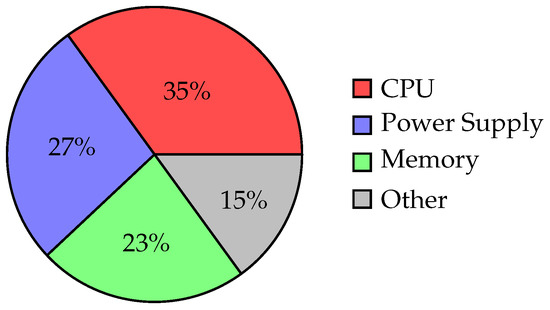
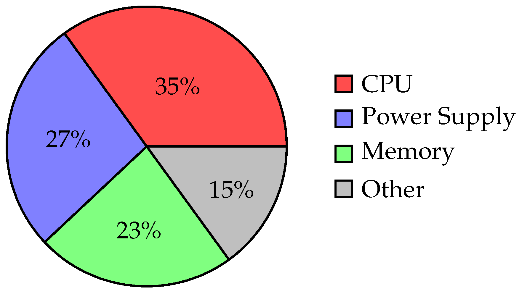
Another promising approach is hardware-enforced power bounding, as discussed in “Beyond DVFS: A First Look at Performance Under a Hardware-Enforced Power Bound” [17]. This technique involves dynamically limiting processor power consumption through mechanisms such as Intel’s Running Average Power Limit (RAPL). By setting power limits, the hardware adjusts CPU performance to remain within the specified power budget, enabling predictable energy use. However, this can cause performance variation due to differences in processor efficiency. Additionally, power clamping emerges as a powerful alternative to traditional DVFS, offering more precise energy management by directly limiting the power a processor can draw during operation. This approach can be dynamically adjusted based on workload demands, thereby ensuring system stability while controlling energy consumption [17]. This is an important consideration as the CPU accounts for over a third of power consumption as shown in Figure 1 [18].

In FPGA-based systems, combining undervolting and overclocking can improve energy efficiency by reducing static and dynamic power consumption while enhancing performance, as shown in [19]. However, this approach risks bit-level faults in critical components like on-chip memory and data paths, requiring robust error correction and hardware design. Moreover, this is a specific use case when most HPC clusters do not feature FPGA devices, and the paper [19] does not consider the impact of following the above on traditional computing systems.

Fine-grained tuning of supply voltages and clock speeds can cut power usage by up to 60% while keeping error rates manageable. Adaptive power management further optimises performance in real-time applications. Similar energy-saving techniques have also been applied to modern HPC processors, achieving significant gains with minimal tuning effort [20].

Another strategy for saving energy is to suspend or power down idle components or nodes using techniques such as sleep modes, Wake on LAN (WoL), or hibernation. As noted in [21], “Since the WoL technology is common in modern PCs, employing EnergySave in networks of PCs can represent a cheap solution that can bring high savings under the energy (kWh), economic (€), and greenhouse gases (tons of CO₂)”. More advanced approaches include Intel’s Demand-Based Switching, which dynamically scales down CPU clock speeds or powers off idle chip regions to reduce power consumption [22].

Incorporating heterogeneous architectures, such as GPUs and other accelerators, alongside traditional CPUs has been shown to enhance energy efficiency in HPC environments. GPUs, designed for parallel processing, offer significant energy savings over CPUs, particularly in applications that benefit from massive parallelism. Studies have demonstrated that for simple computational tasks, GPUs can reduce energy consumption by a factor of 1.1 to 3.2 times compared to CPUs [23]. As the complexity of tasks increases, FPGAs outperform both CPUs and GPUs, achieving energy reduction ratios of 1.2 to 22.3 times for complex vision pipelines [23]. However, these figures come from a study focused on the specific use case of computer vision.

In contrast, CPU-only solutions, while versatile, often consume more energy due to their sequential processing nature, which is often less energy-efficient for workloads that benefit from parallel execution. A holistic approach, like the GreenGPU framework, has been proposed to optimize energy efficiency by dynamically splitting workloads between GPUs and CPUs and by adjusting the frequencies of both components based on their utilization. This method has been shown to achieve up to 21.04% energy savings [24]. By utilising the strengths of each hardware type—GPUs for high-throughput parallel tasks and CPUs for more sequential tasks—heterogeneous architectures can significantly reduce energy consumption without compromising performance. Therefore, integrating GPUs and other accelerators into HPC systems represents a promising direction for achieving green computing goals while maintaining computational power.

2.3. Software Strategies for Reducing Energy Consumption

Software optimisation, coupled with hardware enhancements, is essential. Effective algorithms, particularly in fields such as deep learning, demonstrate the ability to diminish energy usage considerably. Code optimisation can prompt reductions in computation time and, thus, lower energy consumption. Studies have indicated that software-level enhancements may reduce energy consumption by up to 50%, highlighting the latent potential in this area [4]. However, it is important to note that these indications focus on their own software and will vary depending on the software and system in question.

The simple rule that Energy = Power × Time suggests two general ways to save energy: (1) faster speed, given a constant power, and (2) lower power without increasing runtime [25]. This would lead to the belief that in all situations, the processing time can be decreased by increasing performance. However, improving performance and efficiently managing power may conflict with each other because faster speeds frequently result from the use of more resources less efficiently, which may excessively increase power consumption [25].

One software strategy for reducing energy consumption is to use less accurate data types that incur lower resource costs so that the accuracy of data can be sacrificed slightly for improved energy efficiency [26]. Through porting applications such as Monte Carlo Pi to use approximations of nearly all floating-point operations, gains of up to 15% in energy efficiency have been achieved. However, the paper [26] failed to give an example of software for which reducing the accuracy of data may have a larger impact on the correctness of the output, so this should be a consideration in any development plan.

Virtualisation is an effective strategy for partitioning hardware resources, enabling multiple services to run within virtual machines (VMs) on a single physical system. This consolidation increases overall energy efficiency by reducing the need for additional hardware. As multiple VMs share the same hardware, utilisation improves, and energy demands decrease, particularly for cooling, since fewer physical machines are required to deliver the same functionality [22].

At the organisational level, scheduling plays a crucial role in improving the energy efficiency of data centres. Liu et al. explored this by designing an energy-aware scheduler for data-grid systems that support both real-time and data-intensive applications. Their approach considers both the physical location of data and the characteristics of the applications to optimise scheduling decisions. The proposed distributed scheduler integrates task scheduling with data placement strategies to minimise energy usage. Significant energy savings are achieved by reducing unnecessary data replication and limiting task migration across nodes [22,27].

2.4. Energy Measurement and Metrics in Computing

A substantial body of work exists on the measurement and modelling of energy efficiency in computing systems, particularly within high-performance computing (HPC) and data centre contexts. Early work by Hennessy and Patterson [28] formalised the relationship between performance and power through the well-known identity expressed as $Energy=Power\times Time$, highlighting the inherent trade-off between execution speed and energy consumption.

Energy efficiency metrics such as performance per watt have been widely adopted, particularly in benchmarking initiatives such as the Green500 list [29], which ranks supercomputers based on FLOPs per watt. While useful at system scale, such aggregate metrics often obscure workload-specific behaviour and do not capture the interaction between software and hardware optimisation strategies.

More granular approaches have been proposed through power modelling and measurement frameworks. For example, the use of hardware counters and interfaces such as Intel’s Running Average Power Limit (RAPL) enables fine-grained energy measurement at the CPU and memory levels [30]. Similarly, tools such as PowerPack [31] and JouleMeter [32] provide software-based estimation of energy consumption across distributed systems and virtualised environments.

At the application level, several studies have explored energy-delay metrics to capture the trade-off between performance and energy. The Energy-Delay Product (EDP) and Energy-Delay² Product (ED²P) are commonly used composite metrics that penalise both high energy consumption and long execution times [33]. These metrics are particularly relevant when evaluating optimisation strategies where improvements in runtime may come at the cost of increased instantaneous power draw.

In parallel computing, analogous concepts measuring the trade-off of speed against resources to measure “efficiency” exist in the form of speedup and parallel efficiency. Speedup, defined as the ratio of serial to parallel execution time, and efficiency, defined as speedup divided by the number of processors, provide insight into how effectively computational resources are utilised [34].

Despite these advances, there remains a lack of generalisable, workload-agnostic metrics that simultaneously capture energy consumption and performance in a balanced manner. Existing approaches either focus on system-level benchmarking (e.g., FLOPS/W) or introduce composite metrics (e.g., EDP) that may disproportionately weight one dimension. This gap motivates the development of alternative formulations, such as the Energy Factor (EF) and the Efficiency–Performance Score (EPS) proposed in this work, which aim to provide a more interpretable, straightforward, and balanced representation of the energy–performance trade-off that can be applied across heterogeneous optimisation strategies.

2.5. Gaps in the Existing Literature and How This Approach Differs

Despite the depth of research into hardware and software energy-saving techniques, a key gap lies in the lack of empirical studies that examine both in tandem. Most literature treats hardware and software strategies independently, leaving open questions about their combined effects or synergies. Additionally, industry confidentiality often limits access to accurate data on real-world energy consumption and optimisation effectiveness, further complicating cross-layer comparisons. However, it should be considered that this lack of an overarching review may be due to the uniqueness of energy efficiency in individual projects; a problem that is embarrassingly parallelisable may lead to more energy savings than one that requires more sequential operations, for example. In contrast, this review lays the groundwork for an experimental evaluation of cross-layer strategies using a Raspberry Pi cluster, a novel test bed that facilitates real-time measurement and control of both software and hardware parameters.

3. Technical Approach

This section outlines the methodology used to investigate energy efficiency within a small-scale cluster computing environment. The goal is to quantify how software and hardware optimisations affect energy usage and performance using controlled, repeatable experiments.

3.1. Investigating the Problem

As high-performance computing continues to scale, energy consumption has emerged as a critical bottleneck, not just in terms of cost but also in terms of environmental impact. Measuring energy efficiency is no longer optional; it is a necessary step toward sustainable system design. This project seeks to investigate how and why different decisions in software and hardware affect energy usage and whether gains in performance come at the cost of higher power draw. For the purposes of this work, energy efficiency in computing is defined as the change in total energy consumption required completing the same computational workload.

While Raspberry Pis are not directly representative of industrial HPC clusters, they allow for cost-effective, scalable experimentation and are particularly suitable for investigating trends related to parallelisation, energy consumption, and thermal effects. Limitations such as Amdahl’s Law and thermal throttling are considered when interpreting results.

3.2. Assumptions and Experimental Constraints

The voltage supply to the cluster is assumed to be stable at 230 V throughout testing. All tests are conducted with identical operating system images; system load at boot time is minimised, and no background services are allowed to run during workloads. Within the work, we distinguish between compute/node energy, which is measured, and total system-level energy, for example, including cooling, which we do not measure.

The Arduino-based current sensor setup introduces minor latency between sampling and logging, which may slightly affect precision for extremely short workloads. However, due to the averaging of current over longer intervals, the overall effect is expected to be negligible.

In order to ensure a fair and consistent measurement of energy usage, baseline power values were established for the Raspberry Pi cluster at various operational stages. At idle, each Raspberry Pi was observed to draw approximately 3.27 W ± 10%, resulting in a combined idle consumption of around 9.81 W ± 10% for the three-node cluster. These values were calculated using current readings obtained from the SCT-013 current sensor and Arduino setup and confirmed by the Tapo smart plug.

In contrast, when all four CPU cores were fully utilised on each of the three Raspberry Pis (using CPU stress tests), the total power draw increased significantly, ranging between 16 and 18 W. This value represents the system under sustained computational load and serves as the upper bound for evaluating the energy efficiency of software workloads under test conditions.

3.3. Measuring Energy Usage

Quantifying energy usage is essential for evaluating the impact of different software and hardware strategies. In this project, energy consumption is calculated based on electrical power, derived from the product of current and voltage, as shown in Equation (1). The power metric is then combined with execution time (Equation (2)) to determine total energy consumed. For the scale of experiments conducted on the Raspberry Pi cluster, energy usage is most commonly reported in watt hours.

To measure current in real time, a YDHT SCT-013 non-invasive current sensor manufactured by Beijing YaoHuadechang Electronic Co., Ltd. in Beijing, China, is used in conjunction with an Arduino Uno. The sensor clamps onto the live wire of the Raspberry Pi cluster’s power strip and outputs analogue current readings to the Arduino, which are then streamed via serial connection to a coordinating Raspberry Pi node. The accuracy of the SCT-013 sensor was validated by comparing its readings with those from a Tapo smart plug and validated against the expected demand from the hardware specification. The close alignment of values across idle and workload states supports the reliability of the chosen measurement setup.

This measurement pipeline is tightly integrated with a custom job-runner script that automates workload execution and synchronises energy logging. When a job is submitted, the script initiates the energy monitoring process, executes the selected workload (e.g., Monte Carlo Pi), records the runtime, and logs corresponding power readings. These logs are then parsed to compute the average power, total energy consumed, and efficiency metrics such as the Energy Factor (EF) and Efficiency–Performance Score (EPS). This integration enables consistent, low-overhead experimentation and ensures accurate energy tracking across test scenarios.

3.4. Hardware

The experimental setup consists of a Raspberry Pi “bramble” cluster composed of three compute nodes and one coordinator node. Each Raspberry Pi is connected via Ethernet through a central switch to facilitate low-latency communication and synchronised workload distribution. The coordinator Pi also handles energy measurement and logging from the Arduino-based current sensor system. A visual schematic of the cluster setup is shown in Figure 2.

To investigate thermal effects on performance and energy usage, an external cooling fan is used during selected runs. While the Raspberry Pi does not have active cooling by default, under high computational load, the CPU is prone to thermal throttling, which reduces clock frequency and, in turn, performance. Cooling mitigates this throttling, potentially improving runtime but at the cost of additional energy as the nodes are able to perform more computation.

Clock speed is another key hardware variable explored in this study. Underclocking reduces the maximum frequency of the CPU, which theoretically lowers power draw but may lead to longer execution times that negate energy savings. Conversely, overclocking increases performance, potentially reducing runtime and total energy used, provided the increase in power is offset by the decrease in time. However, overclocking may also increase thermal output, leading to throttling or instability if not properly managed. Moreover, as will be encountered later, there are also stability issues when changing the clock speed of components. The Raspberry Pi 3B+ that was employed in this setup has a recommended clock speed of 1.4 GHz, and through testing, operating at 1.6 GHz resulted in system instability on multiple nodes. Therefore, a minimum clock speed of 0.6 GHz to 1.5 GHz was tested.

Another tested strategy is “on-demand computing“, where idle nodes are powered off when not participating in a computation. In principle, this reduces idle energy draw, but in practice, it introduces challenges in coordination, system responsiveness, and reinitialisation time. Additionally, the energy cost of restarting or reconfiguring nodes may outweigh savings from temporary shutdowns in short workloads.

Although Raspberry Pis are not directly comparable to industrial HPC hardware in terms of performance, memory, or thermal management, they provide a scalable and accessible platform for prototyping and controlled experimentation. The insights gained, while not directly transferable in magnitude, are valuable in understanding trends in energy–performance trade-offs and can inform energy-aware practices in larger, more powerful cluster systems.

3.5. Software

Each Raspberry Pi in the cluster runs Raspbian OS Lite, a lightweight Debian-based distribution optimised for performance and minimal overhead. This ensures that background processes do not distort energy measurements. Communication between nodes is handled via Secure Shell (SSH), while distributed workloads are executed using the Message Passing Interface (MPI). For shared-memory parallelism within individual nodes, OpenMP is employed.

The role of software design in energy efficiency is central to this research. Optimisation can occur at several levels—algorithmic (e.g., reducing computational complexity), architectural (e.g., multithreading and workload distribution), and linguistic (e.g., using low-level languages with minimal runtime overhead). To explore these dimensions, all workloads are implemented in both Python and C. While Python offers ease of development and high readability, it introduces significant overhead due to its interpreted nature. In contrast, C provides lower-level memory and execution control, often resulting in faster runtimes and reduced energy consumption.

The Monte Carlo Pi algorithm estimates $\pi$ by generating random points within a square and counting how many fall inside a quarter circle. It is used as the primary benchmark for parallel performance due to its embarrassingly parallel nature. The algorithm scales well across cores and nodes, requiring minimal communication overhead.

To complement this, the recursive Fibonacci algorithm, which computes each term as the sum of the two preceding terms, is used to represent more sequential workloads. Comparing it with Monte Carlo Pi enables an evaluation of how workload parallelisation influences energy efficiency under different configurations.

Graph traversal algorithms, including Breadth-First Search (BFS), which explores nodes level by level; Depth-First Search (DFS), which explores as deep as possible before backtracking; and Dijkstra’s algorithm, which finds the shortest paths from a source node to all others in a weighted graph, are also included. These reflect real-world data-centre workloads such as Web crawling, social network analysis, and routing. Their performance is assessed in both sequential and parallel contexts.

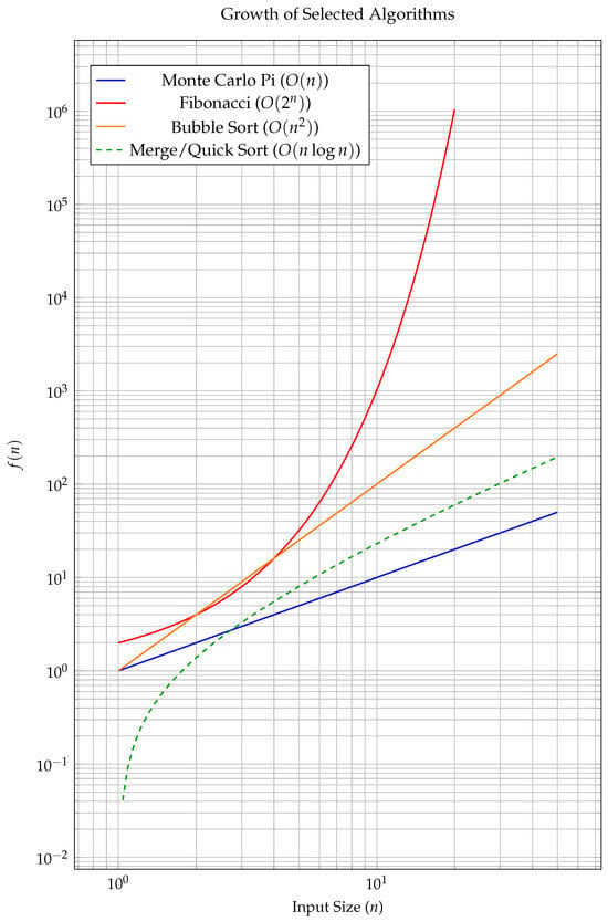
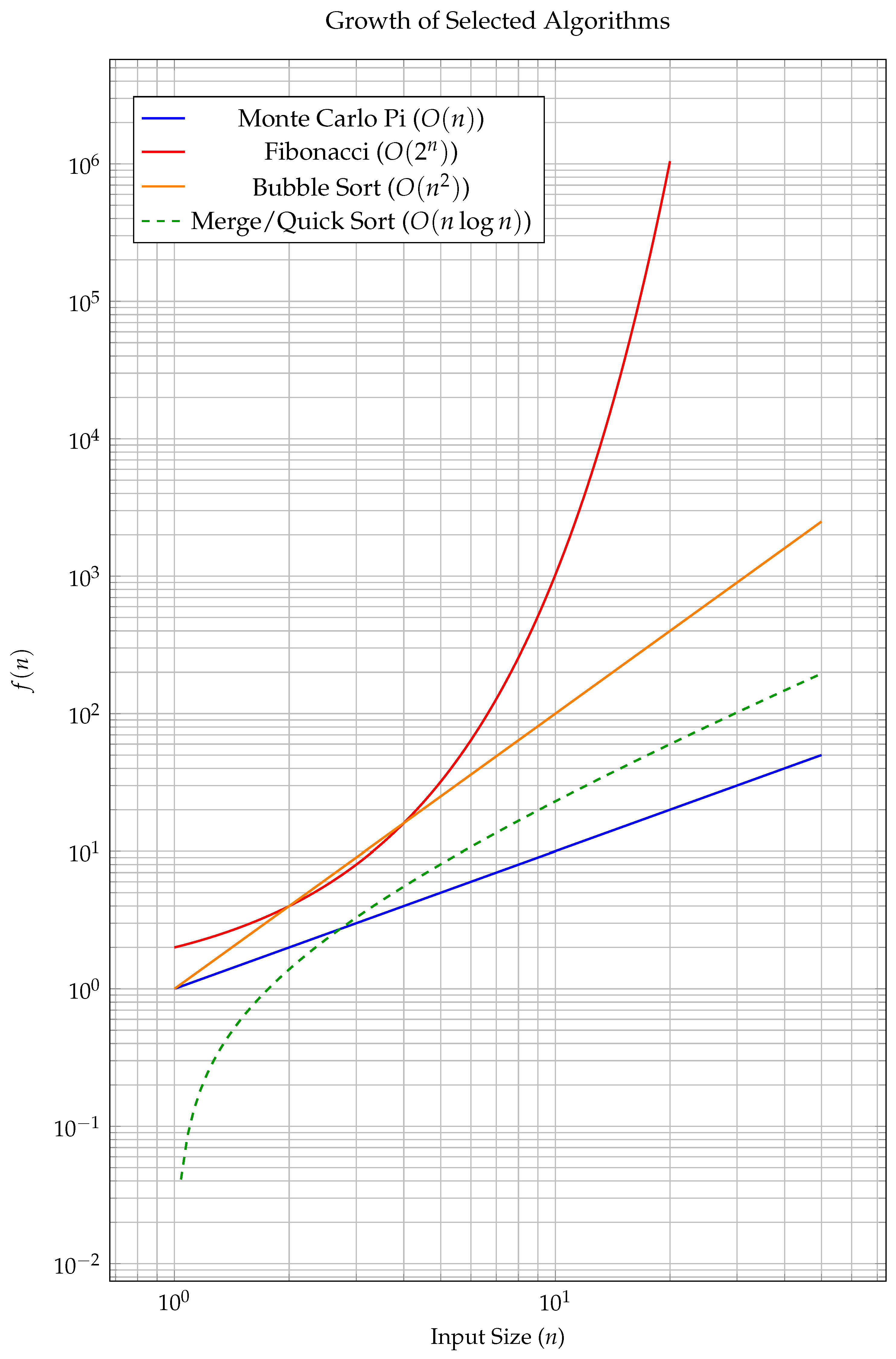
Finally, sorting algorithms such as Bubble Sort, Merge Sort, and Quick Sort are applied to identical randomised arrays. These allow for direct comparisons of energy consumption across different computational complexities. By observing the relationship between input size, algorithmic efficiency (Big-O notation), and actual energy usage, the study reveals how theoretical complexity translates into real-world power consumption.

The variation in algorithmic complexity is visualised in Figure 3.

4. Results and Analysis

4.1. Results

4.1.1. Impact of Language

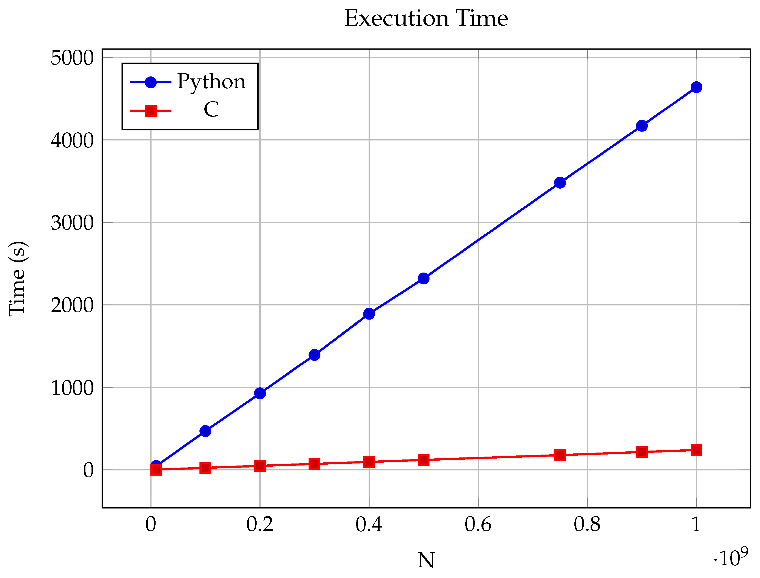
Language choice plays a significant role in the energy efficiency of software. In this project, the same Monte Carlo Pi approximation algorithm was implemented in both Python 3.9 and C (using gcc 15.2) to assess the effect of language-level optimisation on execution time and energy usage. Python, while easy to develop and maintain, is an interpreted language and introduces considerable overhead due to its runtime environment. C, on the other hand, is compiled to native machine code and provides lower-level memory and execution control, resulting in faster runtimes and reduced energy consumption.

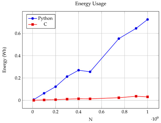
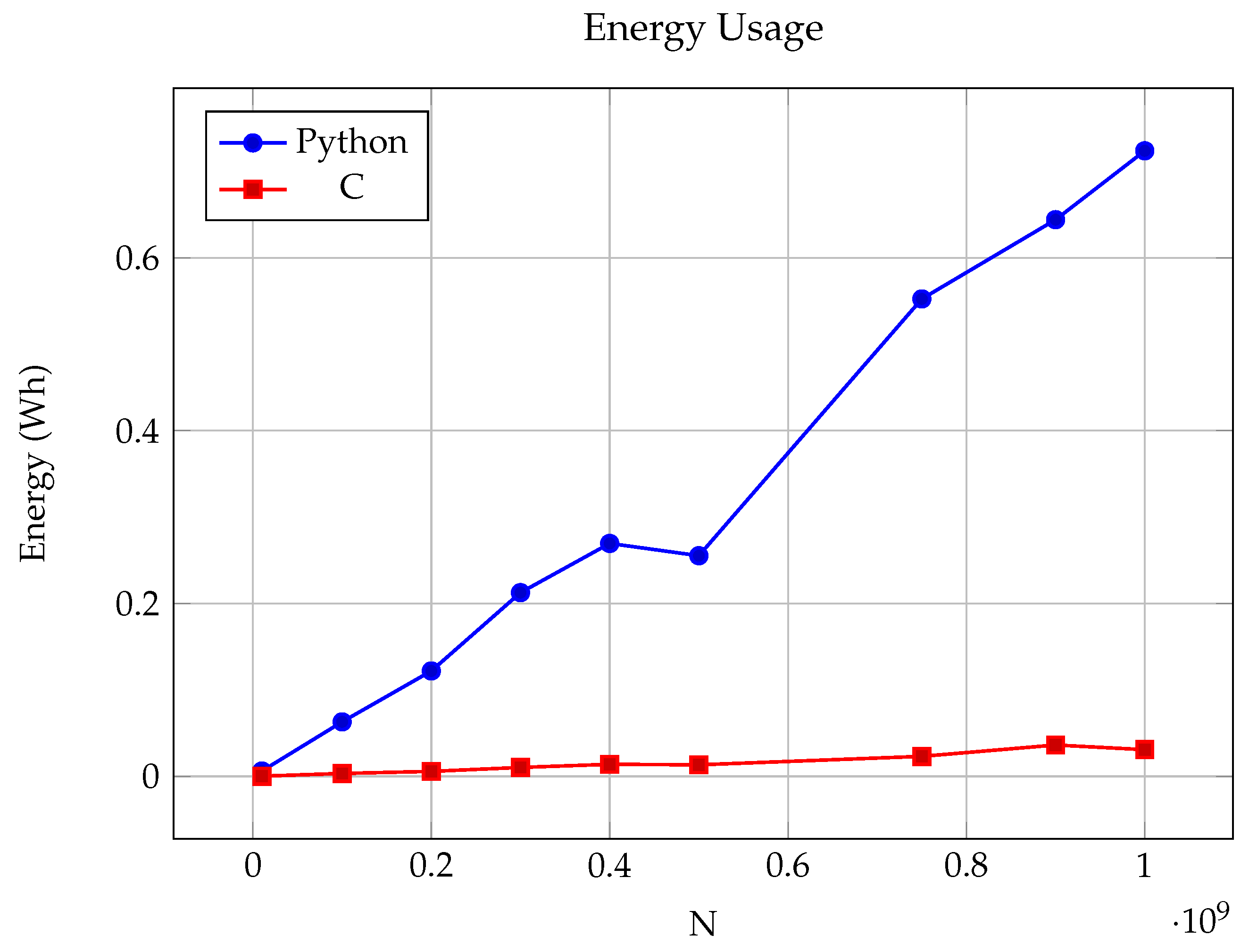
This result highlights that, even for compute-light workloads, compiled languages like C can provide significant energy savings. Over repeated runs or at scale, the efficiency gap between high-level and low-level languages becomes environmentally and financially significant. The results are shown in

Table 1. Monte Carlo Pi—Python results.

N	Time (s)	Energy (Wh)
10 M	46.60	0.0062
100 M	469.61	0.0631
200 M	927.92	0.1220
300 M	1392.86	0.2126
400 M	1892.58	0.2695
500 M	2320.19	0.2553
750 M	3482.23	0.5524
900 M	4171.48	0.6441
1 B	4639.44	0.7238

and

Table 2. Monte Carlo Pi—C results.

N	Time (s)	Energy (Wh)
10 M	2.41	0.0003
100 M	24.01	0.0034
200 M	48.03	0.0058
300 M	72.04	0.0104
400 M	96.08	0.0140
500 M	120.06	0.0134
750 M	178.22	0.0232
900 M	216.19	0.0363
1 B	240.15	0.0309

and Figure 4 and Figure 5.

4.1.2. Impact of Parallelisation

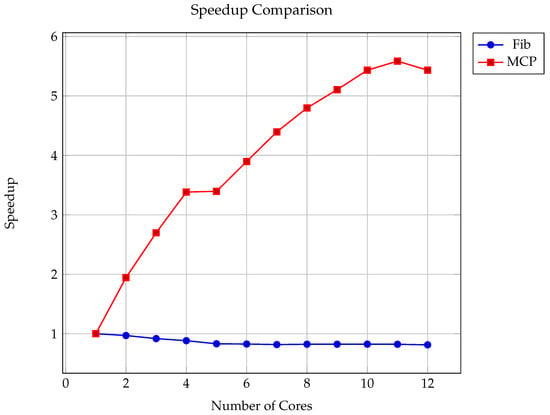
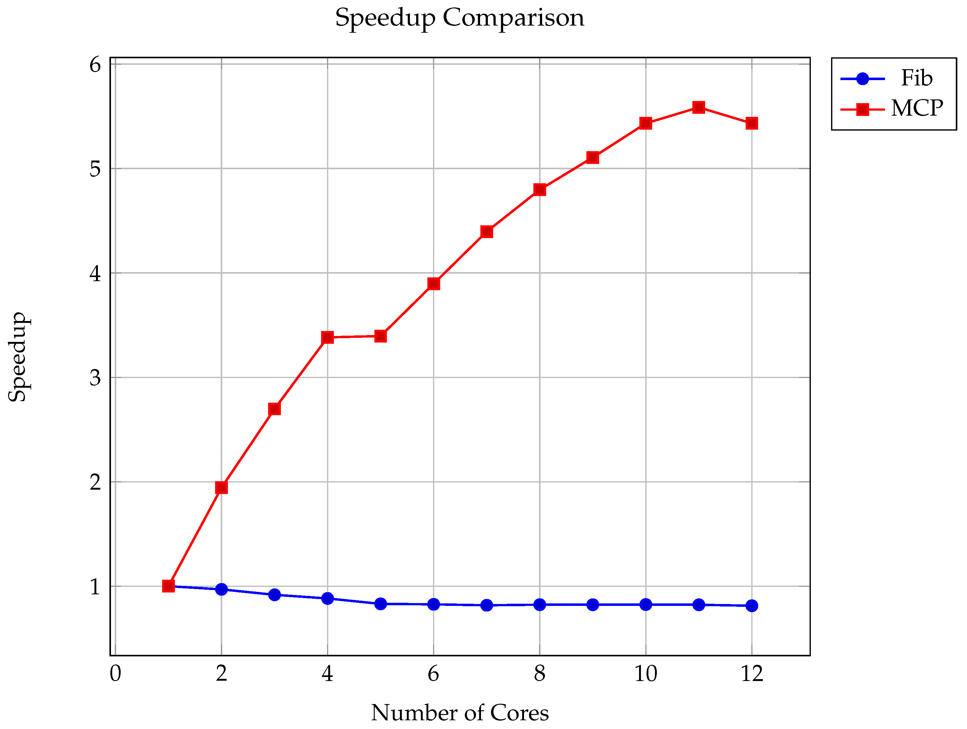
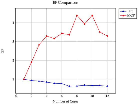
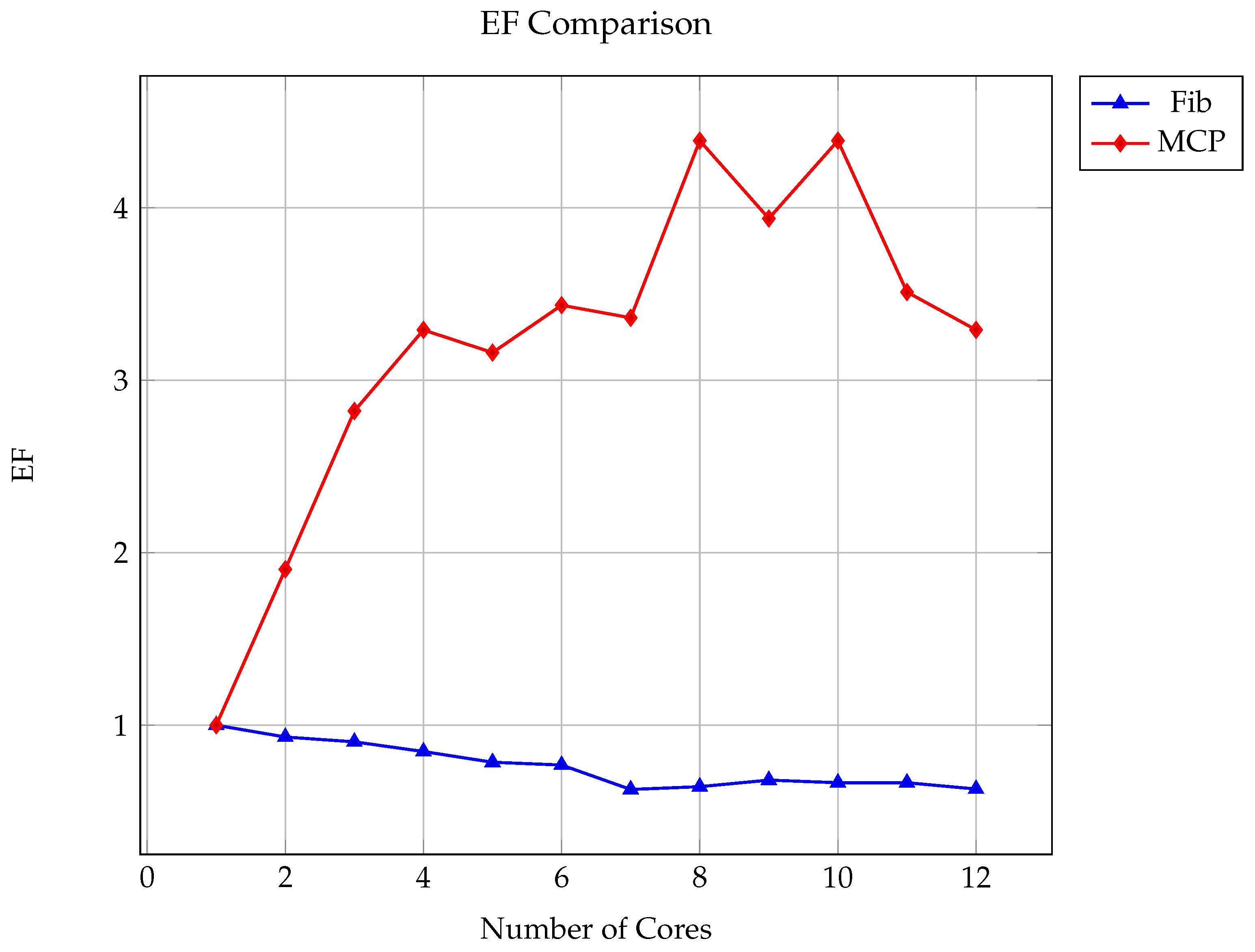
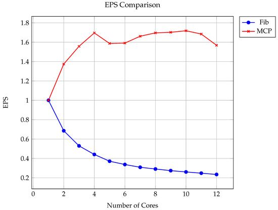
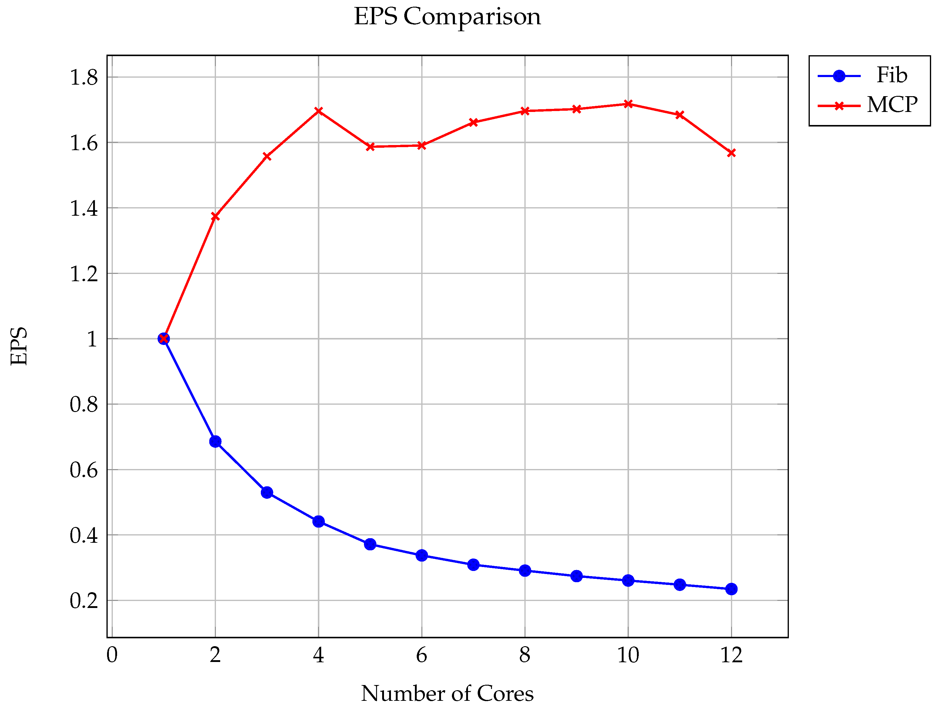
To investigate the role of parallelisation in energy efficiency, two distinct workloads were compared: a non-parallelisable recursive Fibonacci sequence and an embarrassingly parallel Monte Carlo Pi approximation. As the two scripts differ in computational length, their input values were tuned such that the execution time on a single core was approximately the same, providing a fair baseline for comparison. Specifically, fib (1,000,000) took 34.01 s, while a Monte Carlo Pi approximation with 175 million points took 35.69 s on a single core. Once a baseline was established, both workloads were executed across 1 to 12 cores, measuring total time; energy consumed; and derived metrics such as EF, EPS, and parallel efficiency. The results in

Table 3. Monte Carlo Pi for 175,000,000 dots: energy, performance and efficiency metrics.

Processors	Time (s)	Energy (Wh)	Speedup	Parallel Efficiency	EPS
1	35.69	0.070661	1.000	1.000	1.000
2	18.36	0.037119	1.943	0.971	1.375
3	13.23	0.025044	2.698	0.900	1.557
4	10.55	0.021467	3.383	0.845	1.695
5	10.51	0.022361	3.395	0.680	1.586
6	9.16	0.020572	3.896	0.650	1.591
7	8.12	0.021019	4.395	0.628	1.662
8	7.44	0.0161	4.798	0.600	1.696
9	6.99	0.014311	5.106	0.568	1.701
10	6.57	0.0161	5.432	0.543	1.718
11	6.39	0.020125	5.586	0.508	1.684
12	6.57	0.021467	5.432	0.453	1.568

and Figure 6 and Figure 7 clearly show that Monte Carlo Pi benefits significantly from parallelisation. At 12 cores, it achieved a 5.43× speedup and a peak EPS of 1.71, indicating that parallel execution not only reduced runtime but also led to higher energy savings. In contrast, as shown in

Table 4. Fibonacci for 1,000,000 dots: energy, performance and efficiency metrics.

Processors	Time (s)	Energy (Wh)	Speedup	Parallel Efficiency	EPS
1	34.01	0.067083	1.000	1.000	1.000
2	35.07	0.072003	0.970	0.485	0.686
3	37.06	0.074239	0.918	0.306	0.530
4	38.53	0.079158	0.883	0.221	0.441
5	40.94	0.085419	0.830	0.167	0.372
6	41.15	0.087208	0.827	0.138	0.337
7	41.61	0.106886	0.818	0.117	0.309
8	41.32	0.104203	0.823	0.103	0.291
9	41.34	0.098389	0.823	0.091	0.274
10	41.25	0.100625	0.824	0.082	0.261
11	41.36	0.100625	0.822	0.075	0.248
12	41.84	0.106439	0.813	0.068	0.235

Fibonacci achieved diminishing returns as cores increased, speedup actually decreased slightly, and energy usage rose. By 12 cores, Fibonacci’s EPS dropped to just 0.23, compared to Monte Carlo’s 1.57 at the same point. This highlights a key insight: workloads with minimal inter-process communication and independence (like Monte Carlo, where placing dots on a square does not require previous dots or where the other dots are used to calculate Pi) are much more energy-scalable across multiple cores. Conversely, inherently sequential workloads (like Fibonacci recursion) suffer from overhead, resource contention, and idle cycles during parallel execution, making them less suitable for energy-efficient parallelism. It is also observed that while the general trend in the Monte Carlo workload, i.e., that the EPS increases with an increasing number of cores, that due to the smaller workload of 175 million (Monte Carlo Pi can go for much larger values), there is not only a flattening out as the workload approaches 12 cores in terms of EPS, but it can also be seen that there is a decrease for 12 cores, as shown in Figure 8.

4.1.3. Impact of Cooling

Cooling reduces thermal throttling and should, in theory, improve sustained performance. However, any performance gain must be weighed against the fact that cooling systems, themselves, consume additional energy, a factor not measured in this experiment; therefore, it is excluded from the energy analysis but acknowledged as a factor.

In practice, improved cooling may lead to two outcomes: either (1) execution time decreases and, thus, overall energy consumption drops or (2) performance increases at the cost of higher power draw, resulting in greater total energy usage. This section explores this trade-off using two executed Monte Carlo workloads (with $N={10}^9$ and $N={10}^{10}$), comparing cooled vs. non-cooled conditions across core counts ranging from 1 to 12 with results shown in

Table 5. Monte Carlo Pi (N = 1,000,000,000): non-cooled system.

Processors	Time (s)	Energy (Wh)	Speedup	Parallel Eff.	EF	EPS
1	452.37	1.091669	1.000	1.000	1.000	1.000
2	227.78	0.574233	1.986	0.993	1.901	1.943
3	152.67	0.399369	2.963	0.988	2.733	2.846
4	115.97	0.317975	3.901	0.975	3.433	3.659
5	93.23	0.276831	4.852	0.970	3.943	4.374
6	78.50	0.232556	5.763	0.960	4.694	5.201
7	67.07	0.188728	6.745	0.964	5.784	6.246
8	59.25	0.169050	7.635	0.954	6.458	7.022
9	53.01	0.151161	8.534	0.948	7.222	7.850
10	48.05	0.150714	9.414	0.941	7.243	8.258
11	44.09	0.139086	10.260	0.933	7.849	8.974
12	40.06	0.131483	11.292	0.941	8.303	9.683

,

Table 6. Monte Carlo Pi (N = 1,000,000,000): cooled system.

Processors	Time (s)	Energy (Wh)	Speedup	Parallel Eff.	EF	EPS
1	454.08	1.207053	1.000	1.000	1.000	1.000
2	227.88	0.519225	1.993	0.996	2.325	2.152
3	152.87	0.399369	2.970	0.990	3.022	2.996
4	118.82	0.311267	3.822	0.955	3.878	3.850
5	94.04	0.266097	4.829	0.966	4.536	4.680
6	78.37	0.232108	5.794	0.966	5.200	5.489
7	67.46	0.199014	6.731	0.962	6.065	6.389
8	59.33	0.169944	7.653	0.957	7.103	7.373
9	52.89	0.159211	8.585	0.954	7.581	8.068
10	47.38	0.144900	9.584	0.958	8.330	8.935
11	43.58	0.144006	10.419	0.947	8.382	9.345
12	39.82	0.129247	11.403	0.950	9.339	10.320

,

Table 7. Monte Carlo Pi (N = 10,000,000,000): cooled system.

Processors	Time (s)	Energy (Wh)	Speedup	Parallel Eff.	EF	EPS
1	4523.46	13.390281	1.000	1.000	1.000	1.000
2	2263.03	7.438647	1.999	0.999	1.800	1.897
3	1509.00	5.143503	2.998	0.999	2.603	2.794
4	1135.02	3.936897	3.985	0.996	3.401	3.682
5	909.89	3.169017	4.971	0.994	4.225	4.583
6	757.12	2.464642	5.975	0.996	5.433	5.697
7	650.15	2.252658	6.958	0.994	5.944	6.431
8	568.36	1.834953	7.959	0.995	7.297	7.621
9	507.90	1.680661	8.906	0.990	7.967	8.424
10	456.60	1.682897	9.907	0.991	7.957	8.878
11	415.35	1.510717	10.891	0.990	8.864	9.825
12	379.40	1.412775	11.923	0.994	9.478	10.630

and

Table 8. Monte Carlo Pi (N = 10,000,000,000): uncooled system.

Processors	Time (s)	Energy (Wh)	Speedup	Parallel Eff.	EF	EPS
1	4525.15	11.431	1.000	1.000	1.000	1.000
2	2263.54	5.787056	1.999	1.000	1.975	1.987
3	1513.94	4.00085	2.989	0.996	2.857	2.922
4	1157.78	3.659619	3.908	0.977	3.124	3.494
5	922.56	2.802294	4.905	0.981	4.079	4.473
6	766.29	2.482531	5.905	0.984	4.605	5.215
7	657.73	2.043806	6.880	0.983	5.593	6.203
8	583.01	1.939603	7.762	0.970	5.893	6.763
9	518.74	1.697656	8.723	0.969	6.733	7.664
10	467.26	1.550072	9.684	0.968	7.374	8.451
11	424.41	1.390861	10.662	0.969	8.219	9.361
12	389.27	1.400253	11.625	0.969	8.164	9.742

. The motivation for testing this configuration with inputs = ${10}^9$ and ${10}^{10}$ was to increase the time spent in operation, leading to an increased likelihood of thermal throttling; the ability to check whether or not a node is throttling comes from the CLI of that node, which gives the temperature and whether the node is throttling.

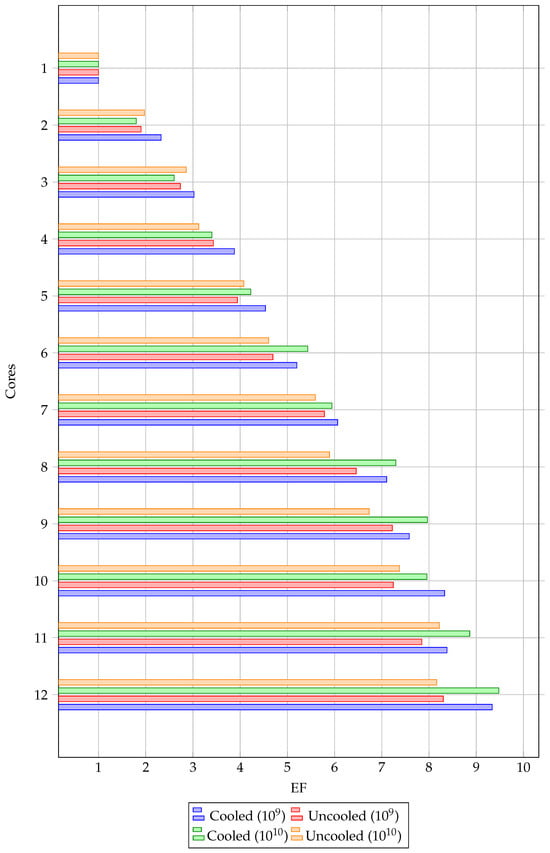
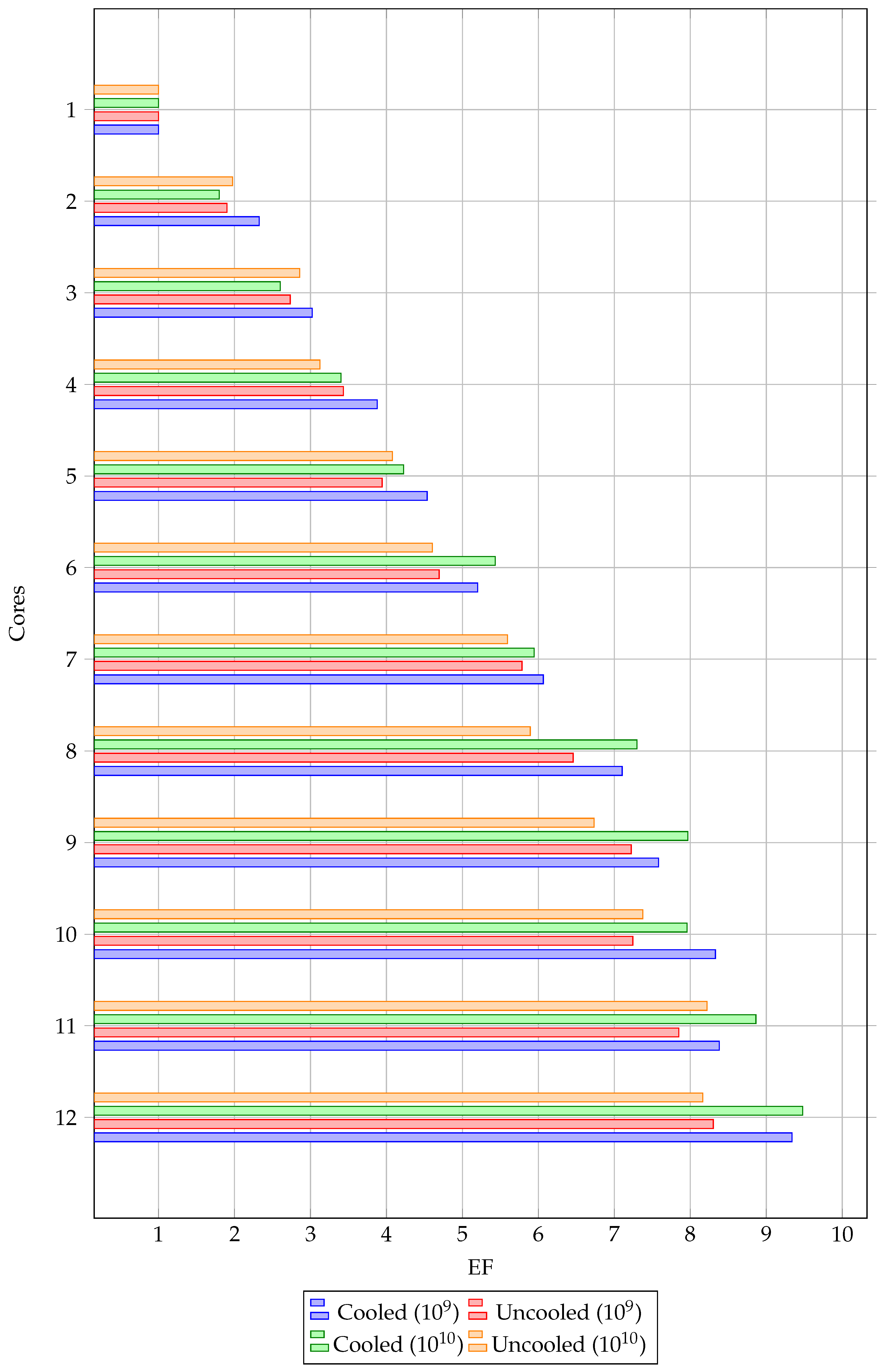
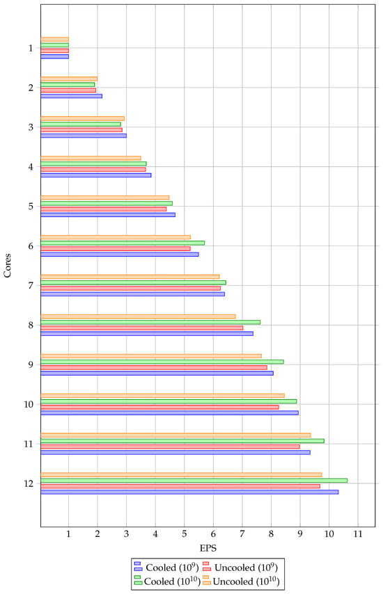
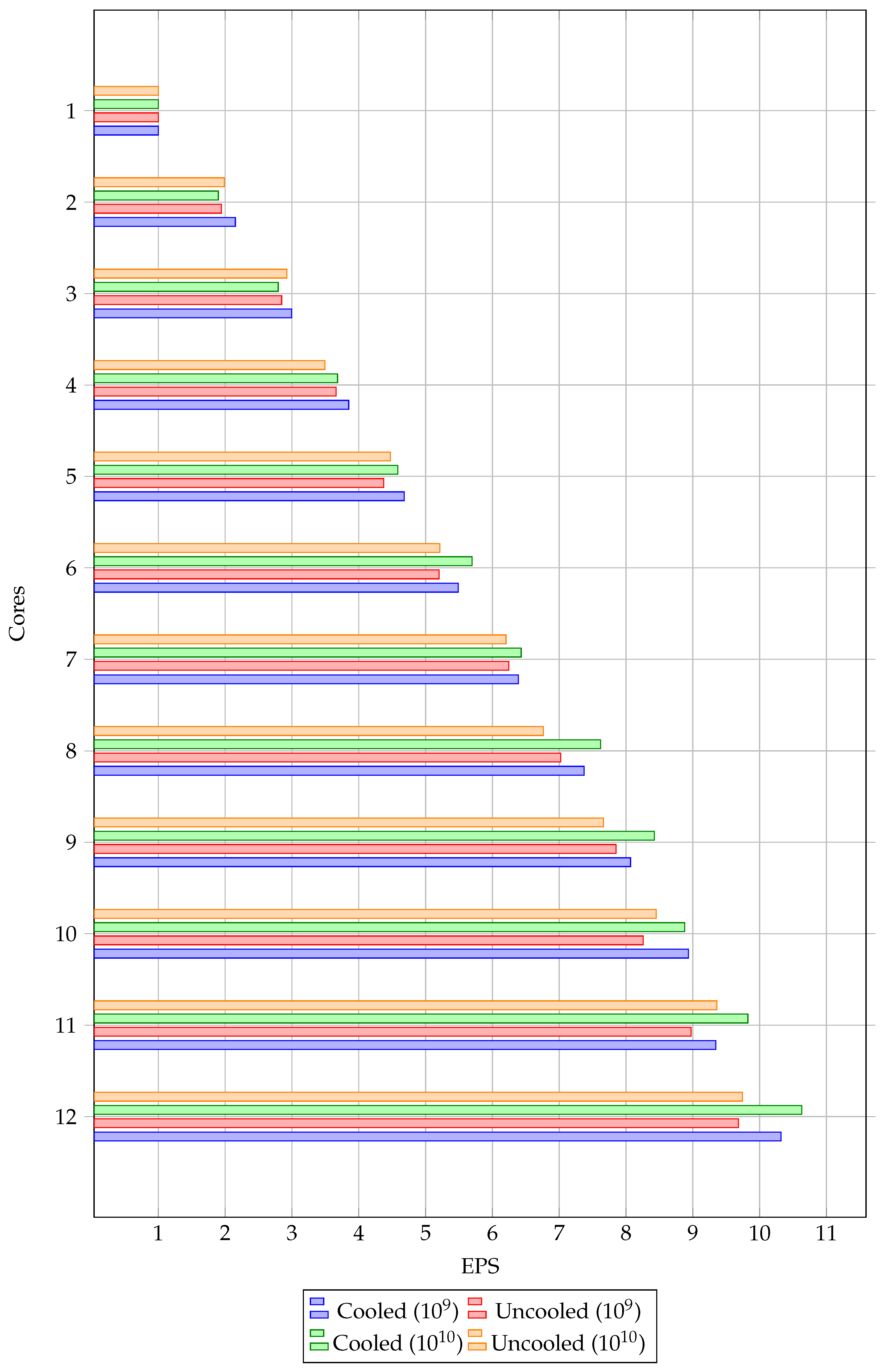
Across the cooled and uncooled workloads for $N={10}^9$, it is evident that there is a slight increase in performance for a growing processor count when the bramble is being cooled. This suggests that while a small number of processors is pegged, this does not massively increase the temperature on the chip; however, when all processors are pegged, the temperature increases to the point where they are throttling and, therefore, gain more of a speedup. For $N={10}^{10}$, this difference is more pronounced, as with increasing amounts of time spent in the workload, there is an increase in the temperature, which causes throttling; as such, cooling the system will result in a better speedup. In terms of EF, as can be viewed in Figure 9, there is a clear trend that for a rising number of processorsthe EF increases, showing an increased energy efficiency for an increasing number of processors; it is clear that the gains found in terms of the decrease in time spent working outweighs the higher energy use through calculations. Moreover, for the EPS in Figure 10, this trend is similar to that of EF; however, as this statistic also takes speedup into account, it can also prove that there is a positive correlation in this case between performance and energy efficiency.

4.1.4. Impact of On-Demand Computing

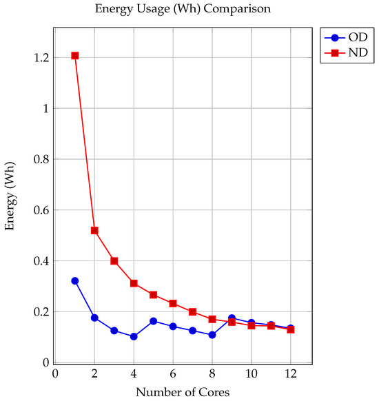
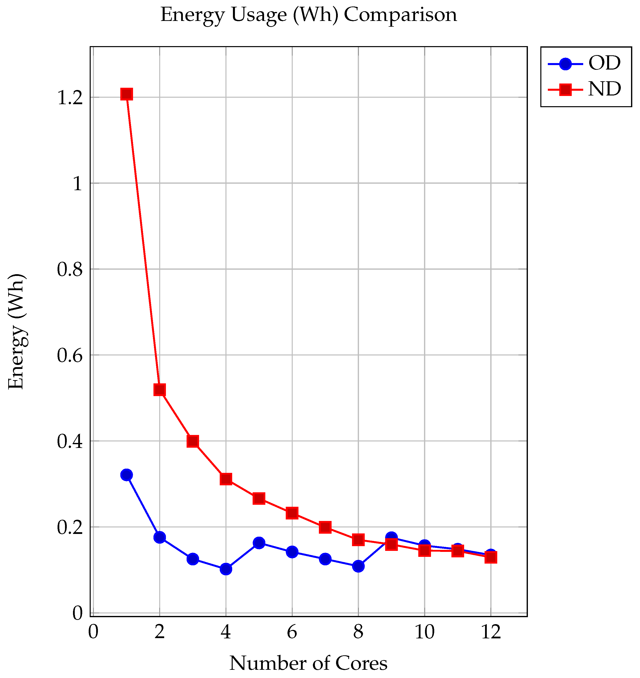
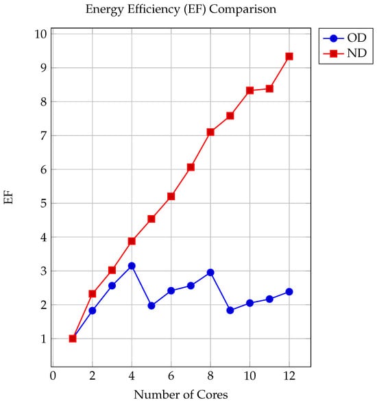
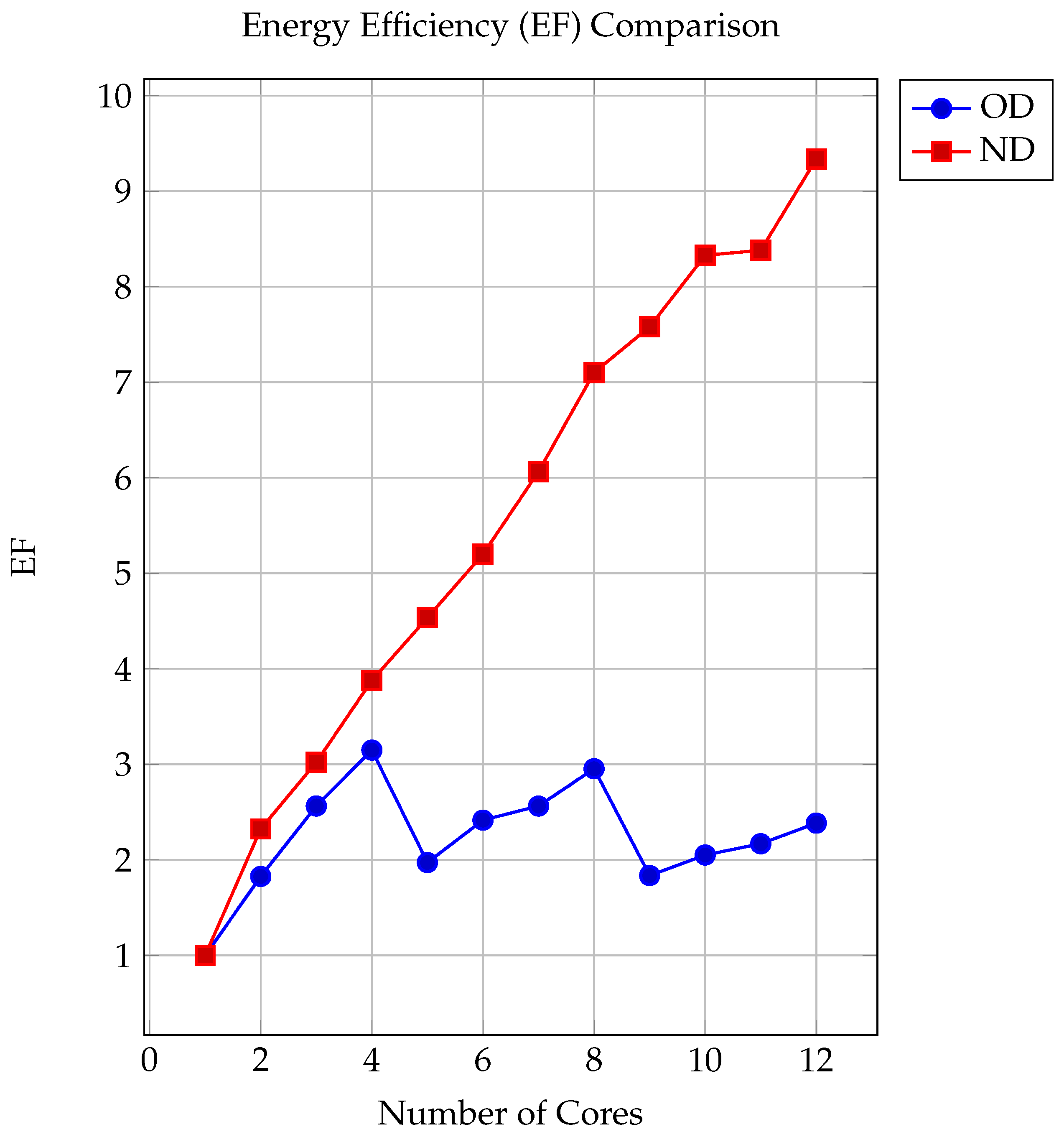
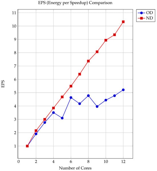
On-demand computing refers to the dynamic powering of nodes only when required rather than keeping all resources powered continuously. While there is some overhead in spinning resources up or down, for predictable workloads with known resource requirements, this model can significantly reduce energy waste from idle components. In terms of pure energy usage, as can be seen in Figure 11, the actual amount of energy used for not powering all three nodes provides a much higher energy savings. However, due to the way that the measurements created for this research operate, i.e., ${\displaystyle \frac{energyon1core}{energyonncores}}$ (where one core is the initial energy requirement and n cores is the new energy requirement), and the EPS, which multiplies speedup and EF due to the much lower starting energy values (due to only powering one node), the EF and EPS for on-demand operation are much lower than those for non-demand operation, even though the trend in speedup is the same. This experiment does show, however, that for workloads that do not require all of the nodes, on-demand computing is a potential solution for energy efficiency with results shown in

Table 9. Monte Carlo Pi (N = 1,000,000,000): on-demand system.

Cores	Time (s)	Energy (Wh)	Speedup	Parallel Eff.	EF	EPS
1	453.76	0.321106	1.000	1.000	1.000	1.000
2	227.81	0.175758	1.9918	0.9959	1.8270	1.9076
3	152.52	0.125222	2.9751	0.9917	2.5643	2.7621
4	116.24	0.101967	3.9036	0.9759	3.1492	3.5061
5	93.57	0.162789	4.8494	0.9699	1.9725	3.0928
6	77.83	0.141769	5.8301	0.9710	2.4165	4.6339
7	66.80	0.125222	6.7921	0.9704	2.5643	4.1736
8	58.73	0.108576	7.7262	0.9658	2.9544	4.7779
9	53.08	0.174864	8.5486	0.9498	1.8363	3.9621
10	47.19	0.156528	9.6156	0.9616	2.0514	4.4414
11	43.20	0.148031	10.5037	0.9549	2.1692	4.7733
12	39.83	0.134614	11.3924	0.9494	2.3854	5.2129

and

Table 10. Monte Carlo Pi (N = 1,000,000,000): non-demand system.

Cores	Time (s)	Energy (Wh)	Speedup	Parallel Eff.	EF	EPS
1	454.08	1.207053	1.000	1.000	1.000	1.000
2	227.88	0.519225	1.9926	0.9963	2.3247	2.1523
3	152.87	0.399369	2.9704	0.9901	3.0224	2.9963
4	118.82	0.311267	3.8216	0.9554	3.8779	3.8496
5	94.04	0.266097	4.8286	0.9657	4.5361	4.6801
6	78.37	0.232108	5.7941	0.9657	5.2004	5.4892
7	67.46	0.199014	6.7311	0.9616	6.0652	6.3895
8	59.33	0.169944	7.6535	0.9567	7.1027	7.3729
9	52.89	0.159211	8.5854	0.9539	7.5815	8.0678
10	47.38	0.144900	9.5838	0.9584	8.3302	8.9351
11	43.58	0.144006	10.4195	0.9472	8.3820	9.3453
12	39.82	0.129247	11.4033	0.9503	9.3391	10.3197

as well as Figure 11, Figure 12 and Figure 13.

4.1.5. Impact of Clocking

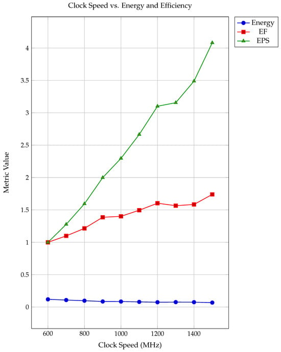
Adjusting the clock speed of processors, either through underclocking or overclocking, offers a direct mechanism to influence both performance and energy consumption. At higher clock speeds, processors can execute instructions more rapidly, reducing the overall execution time. However, this typically comes at the cost of increased power draw per unit time. Conversely, underclocking reduces energy consumption per second but prolongs the execution time of workloads. To investigate this trade-off, a Monte Carlo Pi workload ($N={10}^9$) was executed on all 12 cores of a Raspberry Pi 3B+ cluster under different clock frequencies, ranging from 600 MHz to 1500 MHz. As shown in

Table 11. Impact of clock speed on energy and performance (12 Cores, $N={10}^9$).

Clock Speed (MHz)	Time (s)	Energy (Wh)	Speedup	EF	EPS
600	40.19	0.118961	1.000	1.000	1.000
700	34.62	0.108228	1.1609	1.0992	1.2760
800	30.63	0.097942	1.3121	1.2146	1.5937
900	27.87	0.085867	1.4421	1.3854	1.9978
1000	24.51	0.084972	1.6397	1.4000	2.2956
1100	22.54	0.079606	1.7831	1.4944	2.6645
1200	20.77	0.074239	1.9350	1.6024	3.1007
1300	19.93	0.076028	2.0166	1.5647	3.1553
1400	18.24	0.075133	2.2034	1.5833	3.4887
1500	17.12	0.068425	2.3475	1.7386	4.0814

and Figure 14, increasing the clock speed consistently improved both the speedup and energy efficiency metrics (EF and EPS), indicating that the gains in performance outweighed the rise in energy consumption per second. Notably, the data reveals that the fastest configuration (1500 MHz) resulted in the best EPS value (4.08), suggesting that the shorter execution time more than compensated for the increased instantaneous power draw. The EF metric also increased with clock speed, demonstrating improved energy-to-performance scaling. However, attempts to increase the clock speed beyond 1500 MHz caused instability—devices failed to boot and required reflashing. This limitation highlights a practical ceiling for overclocking on the Raspberry Pi 3B+ hardware used in this study.

4.1.6. Sorting Algorithms and the Impact of Big-O Complexity

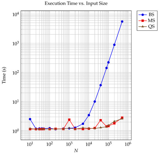
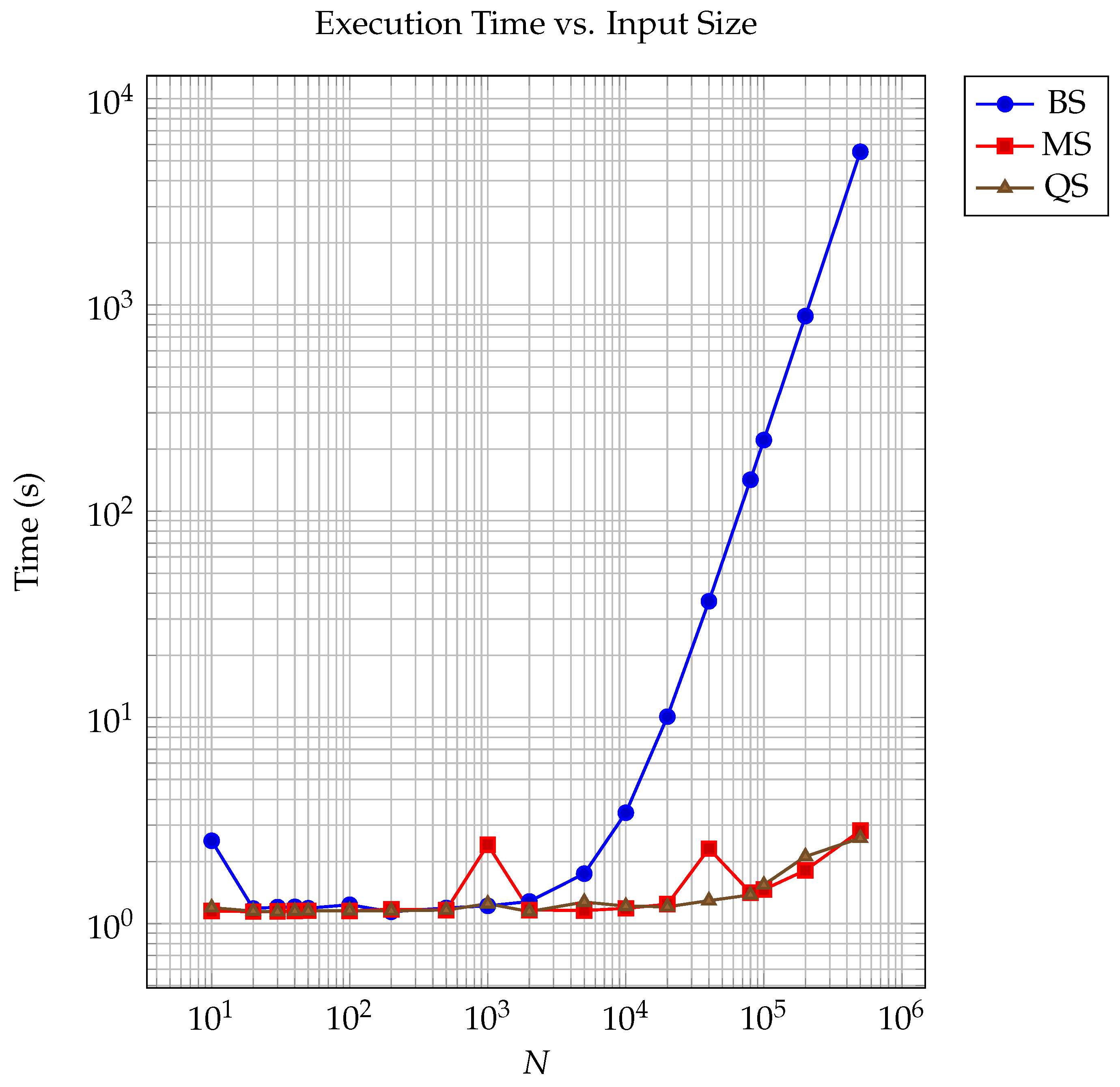
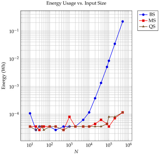
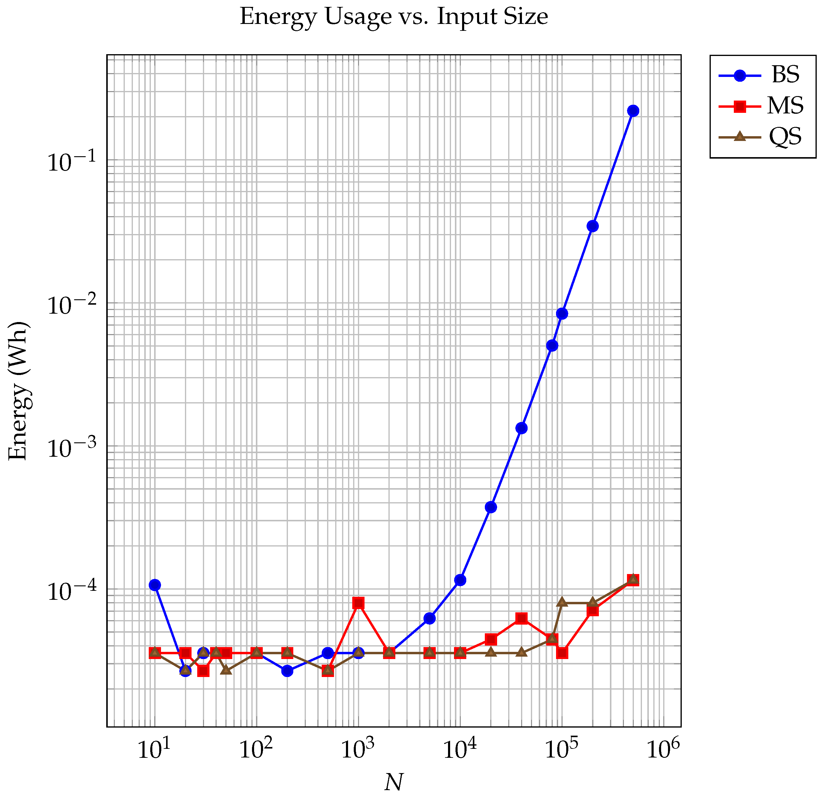
Sorting algorithms were selected to empirically explore how algorithmic complexity impacts both execution time and energy usage. Sorting algorithms provide well-defined theoretical complexities:

• Bubble Sort: $\mathcal{O}\left(n^2\right)$—simple but inefficient;
• Merge Sort: $\mathcal{O}(nlogn)$—efficient;
• Quick Sort: $\mathcal{O}(nlogn)$, on average—fast but can degrade to $\mathcal{O}\left(n^2\right)$.

This made them ideal candidates to test whether energy profiles align with theoretical performance expectations. The results below show that Bubble Sort performs significantly worse than the compared algorithms, with its execution time and energy usage ballooning as the input size N increases. Merge and Quick Sort remain efficient, even with larger N values, both in terms of runtime and Wh consumed. The results (

Table 12. Bubble Sort results.

N	Time (s)	Energy (Wh)
10	2.52	0.000106
100	1.23	0.000036
1000	1.22	0.000036
10,000	3.45	0.000115
50,000	221.27	0.008403
100,000	5531.56	0.220071

,

Table 13. Merge Sort results.

N	Time (s)	Energy (Wh)
10	1.15	0.000036
100	1.15	0.000036
1000	2.41	0.000080
10,000	1.19	0.000036
50,000	1.46	0.000036
100,000	2.82	0.000115

and

Table 14. Quick Sort results.

N	Time (s)	Energy (Wh)
10	1.19	0.000036
100	1.15	0.000036
1000	1.25	0.000036
10,000	1.22	0.000036
50,000	1.54	0.000080
100,000	2.60	0.000115

and Figure 15 and Figure 16 show inconsistencies, as validated in multiple experimentations. At lower values of N, impacts of system or environmental conditions are significant. At higher values of N, as the required computation grows in size, the impact reduces and results become more consistent with what was expected.

4.1.7. Graph Algorithms and the Impact of Traversing an Increasing Number of Nodes

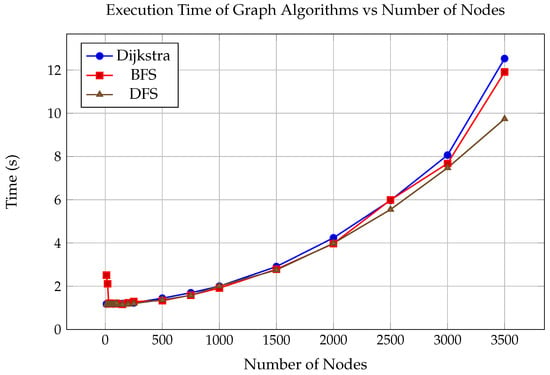
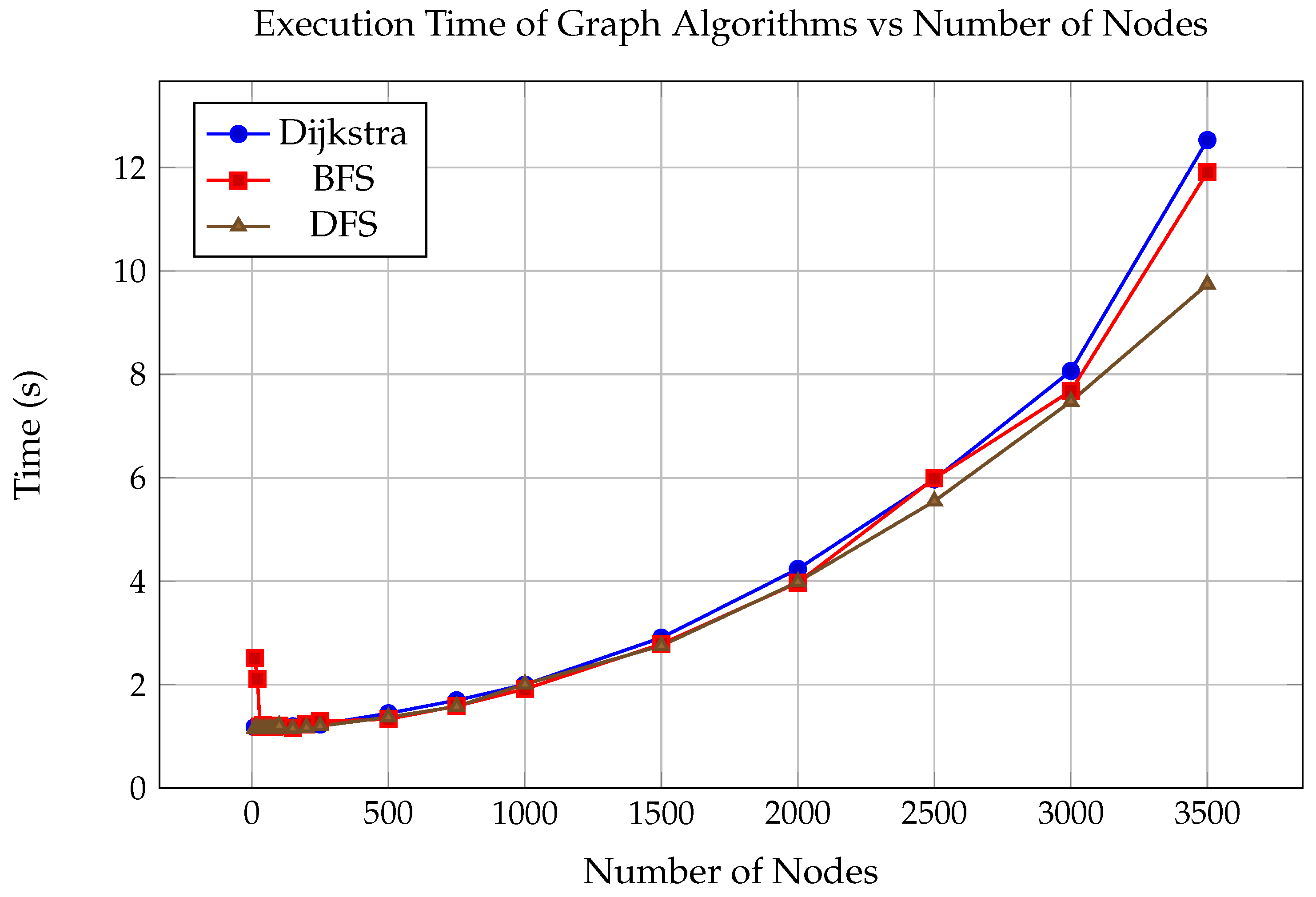
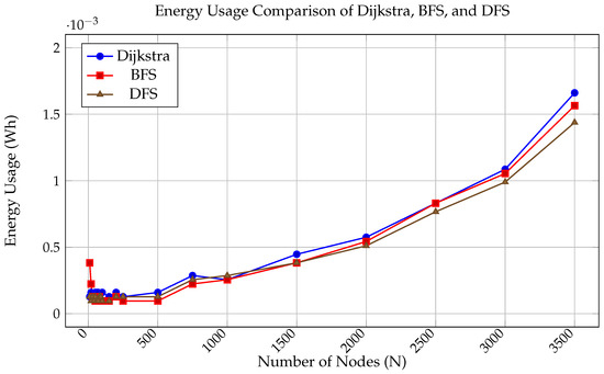
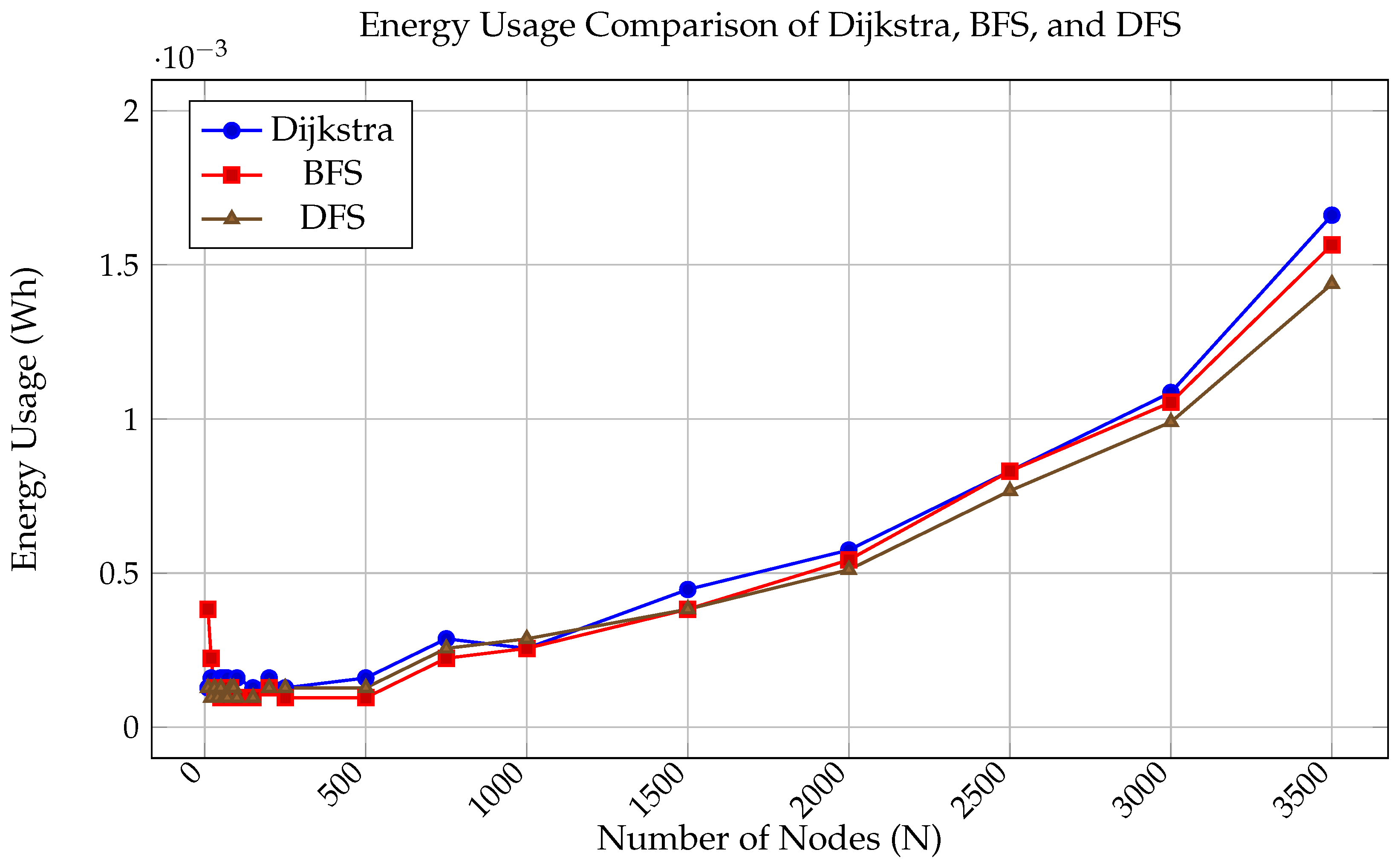
Graph traversal algorithms are critical in many domains of HPC, from network analysis to optimisation problems. This experiment evaluated three classic algorithms—the Dijkstra, Breadth-First Search (BFS), and Depth-First Search (DFS) algorithms—under increasing graph sizes using adjacency matrices.

Due to the memory-intensive nature of storing full adjacency matrices, a hard cap emerged around 4000 nodes. Beyond this point, the Raspberry Pis lacked sufficient memory and killed the process. Therefore, this is the experiment for which there is least amount of accuracy when considering the usage of Pis as an analogue for real HPC nodes. Energy usage remained low across all three algorithms, even as the number of nodes scaled with results shown in Figure 17 and Figure 18 and

Table 15. Dijkstra performance and energy metrics.

N	Time (s)	Energy (Wh)
10	1.1789	0.000128
20	1.2052	0.000160
30	1.1849	0.000128
40	1.2007	0.000128
50	1.1954	0.000160
60	1.1992	0.000160
70	1.1834	0.000160
80	1.1999	0.000128
90	1.1995	0.000096
100	1.1959	0.000160
150	1.1965	0.000128
200	1.2290	0.000160
250	1.2322	0.000128
500	1.4479	0.000160
750	1.6996	0.000287
1000	2.0021	0.000256
1500	2.9090	0.000447
2000	4.2382	0.000575
2500	5.9679	0.000831
3000	8.0646	0.001086
3500	12.5270	0.001661
4000	Killed	–

,

Table 16. BFS performance and energy metrics.

N	Time (s)	Energy (Wh)
10	2.5136	0.000383
20	2.1134	0.000224
30	1.1911	0.000128
40	1.2128	0.000128
50	1.1862	0.000096
60	1.2095	0.000096
70	1.1935	0.000096
80	1.1874	0.000128
90	1.1957	0.000096
100	1.2112	0.000096
150	1.1629	0.000096
200	1.2360	0.000128
250	1.2929	0.000096
500	1.3342	0.000096
750	1.5888	0.000224
1000	1.9163	0.000256
1500	2.7859	0.000383
2000	3.9720	0.000543
2500	5.9881	0.000831
3000	7.6786	0.001054
3500	11.9069	0.001565
4000	Killed	–

and

Table 17. DFS performance and energy metrics.

N	Time (s)	Energy (Wh)
10	1.1534	0.000128
20	1.1674	0.000096
30	1.1405	0.000128
40	1.1411	0.000096
50	1.1619	0.000128
60	1.1507	0.000096
70	1.1452	0.000096
80	1.1554	0.000128
90	1.1531	0.000128
100	1.2112	0.000096
150	1.1565	0.000096
200	1.1732	0.000128
250	1.2010	0.000128
500	1.3737	0.000128
750	1.5797	0.000256
1000	2.0100	0.000287
1500	2.7529	0.000383
2000	3.9876	0.000511
2500	5.5474	0.000767
3000	7.4741	0.000990
3500	9.7381	0.001438
4000	Killed	–

. This reinforces the idea that well-designed algorithms with efficient data-access patterns can perform admirably to provide energy savings.

4.2. Analysis

This research confirms that energy efficiency and performance are deeply linked but not always in straightforward ways. Across all experiments, performance optimisations, whether via compiled languages, parallelisation, or overclocking, generally led to improved energy efficiency. Notably, the Monte Carlo Pi workload achieved a 4× improvement in EPS when moving from Python to C and an improvement of over 5× in EPS when parallelised across 12 cores. These results underscore the impact of well-matched workloads and system configurations.

However, the study also highlights that speed and efficiency are not always synonymous. For workloads like recursive Fibonacci operation, increased parallelism led to worse energy metrics, showing that not all workloads lead to gains to justify their energy cost when parallelised. This pattern repeated with clocking experiments: overclocking offered significant speedups and energy gains up to a point, beyond which system instability prevented further gains.

Importantly, system-level strategies like cooling and on-demand computing demonstrated meaningful improvements, especially under heavy workloads. Cooling mitigated thermal throttling, resulting in smoother scaling, while on-demand computing significantly reduced overall energy usage.

Crucially, this study reveals an under-appreciated cost in energy-aware software development: developer time and skill. Writing parallel, efficient code for workloads that are not embarrassingly parallelisable is difficult. The benefit of such optimisation is only worthwhile when the workload is performed frequently or at scale; otherwise, the human and financial cost of optimisation may outweigh the energy savings. While our work focusses on small clusters and is not completely generalisable, the same challenge exists for real-world HPC and green computing: balancing development overhead with sustainability goals.

Moreover, the findings of this project emphasise the need to embed energy awareness into the early stages of system design and software development. As energy costs rise and environmental concerns grow, future computing systems, from data centres to edge devices, will need to be optimised not only for performance but also for energy efficiency in every layer. This research reinforces the value of empirical testing over assumptions, showing that even small-scale, low-power clusters can reveal meaningful insights about workload behaviour. Encouragingly, it also shows that many gains can be achieved through software and configuration alone, offering a low-barrier entry point to greener computing without requiring expensive new hardware.

5. Conclusions

5.1. Summary of Findings

• Programming Language: The choice of programming language had a notable impact on energy efficiency and execution time. C, a compiled language, significantly outperformed Python in both metrics, demonstrating that lower-level languages offer measurable energy savings, particularly for repetitive or computationally intensive workloads like Monte Carlo Pi.
• Parallelisation and Multi-node Execution: Parallelisation greatly improved both performance and energy efficiency—but only when applied to suitable workloads. Monte Carlo Pi, being embarrassingly parallel, showed strong scaling across up to 12 cores, with increased EPS and EF. However, recursive Fibonacci, a sequential workload, suffered from increased energy usage and reduced EPS when parallelised, showcasing the importance of workload profiling before parallel implementation.
• Cooling: Cooling hardware led to noticeable improvements in both runtime and energy usage under high loads. For large workloads ($N={10}^9$ and $N={10}^{10}$), cooled systems exhibited better EPS and EF compared to uncooled ones, confirming that thermal throttling on small devices like Raspberry Pis can significantly impact performance and efficiency.
• Clock Speed: Overclocking provided clear benefits up to a safe threshold (1500 MHz), improving execution time while maintaining or even improving energy efficiency. Higher speeds reduced the time processors were active, which outweighed the increase in instantaneous power draw—making overclocking an effective, low-effort optimisation.
• EF & EPS: EF and EPS proved to be reliable metrics for comparing energy–performance trade-offs. Across most experiments, particularly for Monte Carlo and sorting workloads, EF aligned well with speedup trends. However, in on-demand configurations or when parallelising inefficient workloads, EF and EPS exposed energy waste hidden by performance metrics alone.
• Generalization of Findings: The work presented here is a framework for the measurement of energy use and quantification of changes in that energy use. While the formulae and approaches, in general, can be widely applied, the experimental work to validate these was performed on a small cluster, which limits the wider applicability of the specific experimental findings as discussed in Section 5.3.

5.2. Key Takeaways

• Energy efficiency and performance are not always aligned. Effective optimisation requires the matching of system design with workload characteristics.
• Parallelisation offers strong gains for suitable workloads but wastes energy if applied blindly.
• Simple system-level interventions, like cooling and clock tuning, may offer tangible energy savings with little development overhead.
• Programming languages and algorithmic choices impact energy usage as much as runtime, emphasising the importance of considering both hardware and software layers in sustainable system design.
• Metrics like EF and EPS are essential in comparing energy–performance trade-offs and can reveal inefficiencies that raw speedup fails to capture.

5.3. Limitations and Potential Future Work

• This research was conducted over a limited time scale, and future work could yield further insights through more detailed and extensive experimentation.
• The test bed consisted of three Raspberry Pi 3B+ nodes, which are not representative of the complexity, scale, and thermal behaviour of real-world HPC clusters or data centres. For example, the memory limitations of the experimental setup capped the graph size at 4000 nodes, showing that while this work is indicative of power impacts, it may not directly relate to full HPC environments.
• Experimentation considering cooling did not measure or account for the power of active cooling (fan power draw), which limits how applicable the results on cooling may be; however, as the cooling method was highly inefficient and analysis of different methods is outside the scope of this work, it remains indicative of what could be achieved.
• The energy data was interpreted with some support from real-world cost and emission statistics, which, while taken from reputable sources, could not all be explicitly verified or cited.
• In the future, these experiments should be replicated on a larger HPC cluster to validate trends and scaling behaviours more accurately.
• Consideration of CPython or other approaches to speeding up python execution could be undertaken beyond consideration of only interpreted code.
• Exploration of heterogeneous architectures, such as GPUs, FPGAs, and emerging technologies like quantum accelerators, would offer valuable insight into whether they can complete specific workloads in a more energy-efficient manner than traditional CPUs.
• Future work could also investigate automated tools for software-level optimisation, including compilers or profiling tools that recommend low-energy implementations.

References

- International Energy Agency. Data Centres and Data Transmission Networks; Tracking Report; IEA: Paris, France, 2022. [Google Scholar]
- van Kempen, N.; Kwon, H.J.; Nguyen, D.T.; Berger, E.D. It’s not Easy Being Green: On the Energy Efficiency of Programming Languages. arXiv 2025, arXiv:2410.05460. [Google Scholar] [CrossRef] [Scilit]
- Jiang, H.; Xiong, F.; Huang, Y. Energy efficiency improvement scheme based on edge computing. In Proceedings of the 2021 IEEE International Conference on Artificial Intelligence and Computer Applications (ICAICA); IEEE: New York, NY, USA, 2021; pp. 1033–1036. [Google Scholar] [CrossRef] [Scilit]
- Masciari, E.; Napolitano, E.V. The Environmental Cost of High Performance Computing System Simulation. In Proceedings of the 2024 32nd Euromicro International Conference on Parallel, Distributed and Network-Based Processing (PDP); IEEE: New York, NY, USA, 2024; pp. 289–292. [Google Scholar] [CrossRef] [Scilit]
- Paul, S.G.; Saha, A.; Arefin, M.S.; Bhuiyan, T.; Biswas, A.A.; Reza, A.W.; Alotaibi, N.M.; Alyami, S.A.; Moni, M.A. A Comprehensive Review of Green Computing: Past, Present, and Future Research. IEEE Access 2023, 11, 87445–87494. [Google Scholar] [CrossRef] [Scilit]
- Top 500 Green 500. Top 500 Green 500 November 2024. Available online: https://top500.org/lists/green500/2024/11/ (accessed on 23 March 2025).
- Department for Energy Security and Net Zero. Valuation of Energy Use and Greenhouse Gas Emissions; Technical Report; UK Government: London, UK, 2023.
- International Energy Agency (IEA). CO2 Emissions in 2023: Executive Summary; IEA: Paris, France, 2023. [Google Scholar]
- Strubell, E.; Ganesh, A.; McCallum, A. Energy and policy considerations for modern deep learning research. In Proceedings of the AAAI Conference on Artificial Intelligence; AAAI: Washington, DC, USA, 2020; Volume 34, pp. 13693–13696. [Google Scholar]
- Amazon Web Services. Carbon-Free Energy. 2025. Available online: https://sustainability.aboutamazon.com/products-services/aws-cloud#:~:text=a%20new%20tab-,Carbon%2Dfree%20energy,of%20our%20original%202030%20goal (accessed on 23 March 2025).
- Masciari, E.; Napolitano, E.V. Environmental Sustainability of AI: Estimating $$CO_2$$e Emissions Across Cloud, Edge, and Fog Paradigms. In Proceedings of the Web Information Systems Engineering—WISE 2024 PhD Symposium, Demos and Workshops; Barhamgi, M., Wang, H., Wang, X., Aïmeur, E., Mrissa, M., Chikhaoui, B., Boukadi, K., Grati, R., Maamar, Z., Eds.; Springer: Berlin/Heidelberg, Germany, 2025; pp. 409–418. [Google Scholar]
- Argerich, M.F.; Patiño-Martínez, M. Measuring and Improving the Energy Efficiency of Large Language Models Inference. IEEE Access 2024, 12, 80194–80207. [Google Scholar] [CrossRef] [Scilit]
- Samsi, S.; Zhao, D.; McDonald, J.; Li, B.; Michaleas, A.; Jones, M.; Bergeron, W.; Kepner, J.; Tiwari, D.; Gadepally, V. From Words to Watts: Benchmarking the Energy Costs of Large Language Model Inference. In Proceedings of the 2023 IEEE High Performance Extreme Computing Conference (HPEC); IEEE: New York, NY, USA, 2023; pp. 1–9. [Google Scholar] [CrossRef] [Scilit]
- Eurostat. Electricity Price Statistics—Statistics Explained. 2024. Available online: https://ec.europa.eu/eurostat/statistics-explained/index.php?title=Electricity_price_statistics#Electricity_prices_for_non-household_consumers (accessed on 23 March 2025).
- U.S. Bureau of Labor Statistics. Average Energy Prices, Selected Areas, Midwest Region. 2024. Available online: https://www.bls.gov/regions/midwest/data/averageenergyprices_selectedareas_table.htm (accessed on 22 March 2025).
- Statista. China: Business Electricity Price 2024. Available online: https://www.statista.com/statistics/1373596/business-electricity-price-china/ (accessed on 23 March 2025).
- Rountree, B.; Ahn, D.H.; de Supinski, B.R.; Lowenthal, D.K.; Schulz, M. Beyond DVFS: A First Look at Performance under a Hardware-Enforced Power Bound. In Proceedings of the 2012 IEEE 26th International Parallel and Distributed Processing Symposium Workshops and PhD Forum; IEEE: New York, NY, USA, 2012; pp. 947–953. [Google Scholar] [CrossRef] [Scilit]
- Labasan, S. Energy-Efficient and Power-Constrained Techniques for Exascale Computing; Semanticscholar: Seattle, WA, USA, 2016. [Google Scholar]
- Wu, Y.; Mota, J.F.C.; Wallace, A.M. Joint Undervolting and Overclocking Power Scaling Approximation on FPGAs. In Proceedings of the 2022 Sensor Signal Processing for Defence Conference (SSPD); IEEE: New York, NY, USA, 2022; pp. 1–5. [Google Scholar] [CrossRef] [Scilit]
- Calore, E.; Gabbana, A.; Schifano, S.F.; Tripiccione, R. Evaluation of DVFS techniques on modern HPC processors and accelerators for energy-aware applications. Concurr. Comput. Pract. Exp. 2017, 29, e4143. [Google Scholar] [CrossRef] [Scilit]
- Ricciardi, S.; Santos-Boada, G.; Careglio, D.; Palmieri, F.; Fiore, U. Evaluating energy savings in WoL-enabled networks of PCs. In Proceedings of the 2013 IEEE International Symposium on Industrial Electronics; IEEE: New York, NY, USA, 2013; pp. 1–6. [Google Scholar] [CrossRef] [Scilit]
- Wang, J.; Feng, L.; Xue, W. A review of energy efficiency technology in computer servers and cluster systems. In Proceedings of the 2011 3rd International Conference on Computer Research and Development; IEEE: New York, NY, USA, 2011; Volume 2, pp. 109–113. [Google Scholar] [CrossRef] [Scilit]
- Qasaimeh, M.; Denolf, K.; Lo, J.; Vissers, K.; Zambreno, J.; Jones, P.H. Comparing energy efficiency of CPU, GPU and FPGA implementations for vision kernels. In Proceedings of the 2019 IEEE International Conference on Embedded Software and Systems (ICESS); IEEE: New York, NY, USA, 2019; pp. 1–8. [Google Scholar]
- Ma, K.; Li, X.; Chen, W.; Zhang, C.; Wang, X. Greengpu: A holistic approach to energy efficiency in gpu-cpu heterogeneous architectures. In Proceedings of the 2012 41st International Conference on Parallel Processing; IEEE: New York, NY, USA, 2012; pp. 48–57. [Google Scholar]
- Jin, C.; de Supinski, B.R.; Abramson, D.; Poxon, H.; DeRose, L.; Dinh, M.N.; Endrei, M.; Jessup, E.R. A survey on software methods to improve the energy efficiency of parallel computing. Int. J. High Perform. Comput. Appl. 2017, 31, 517–549. [Google Scholar] [CrossRef] [Scilit]
- Sampson, A.; Dietl, W.; Fortuna, E.; Gnanapragasam, D.; Ceze, L.; Grossman, D. EnerJ: Approximate data types for safe and general low-power computation. In Proceedings of the PLDI ’11: 32nd ACM SIGPLAN Conference on Programming Language Design and Implementation; ACM: New York, NY, USA, 2011; pp. 164–174. [Google Scholar] [CrossRef] [Scilit]
- Liu, C.; Qin, X.; Kulkarni, S.; Wang, C.; Li, S.; Manzanares, A.; Baskiyar, S. Distributed Energy-Efficient Scheduling for Data-Intensive Applications with Deadline Constraints on Data Grids. In Proceedings of the 2008 IEEE International Performance, Computing and Communications Conference; IEEE: New York, NY, USA, 2008; pp. 26–33. [Google Scholar] [CrossRef] [Scilit]
- Hennessy, J.L.; Patterson, D.A. Computer Architecture: A Quantitative Approach; Morgan Kaufmann; Elsevier: Amsterdam, The Netherlands, 2011. [Google Scholar]
- The Green 500 List: Encouraging Sustainable Supercomputing. In Computer; IEEE: New York, NY, USA, 2007; Volume 40, No. 12, pp. 50–55.
- David, H.; Gorbatov, E.; Hanebutte, U.R.; Khanna, R.; Le, C. RAPL: Memory power estimation and capping. In Proceedings of the 16th ACM/IEEE International Symposium on Low Power Electronics and Design, Austin, TX, USA, 18–20 August 2010. [Google Scholar]
- Ge, R.; Feng, X.; Song, S.; Chang, H.C.; Cameron, K.W. PowerPack: Energy profiling and analysis of high-performance systems and applications. IEEE Trans. Parallel Distrib. Syst. 2010, 21, 658–671. [Google Scholar] [CrossRef] [Scilit]
- Kansal, A.; Zhao, F.; Liu, J.; Kothari, N.; Bhattacharya, A.A. Joulemeter: Automated power measurement of data center workloads. In Proceedings of the 1st ACM Symposium on Cloud Computing, Indianapolis, IN, USA, 10–11 June 2010. [Google Scholar]
- Van den Steen, S.; Eyerman, S.; Eeckhout, L.; John, L.K. SWEEP: Evaluating Computer System Energy Efficiency. In Proceedings of the 6th International Conference on High Performance and Embedded Architectures and Compilers (HiPEAC), Heraklion, Greece, 23–25 January 2011; pp. 367–376. [Google Scholar]
- Amdahl, G.M. Validity of the single processor approach to achieving large scale computing capabilities. In Proceedings of the AFIPS Conference Proceedings, Atlantic City, NJ, USA, 18–20 April 1967. [Google Scholar]
Disclaimer/Publisher’s Note: The statements, opinions and data contained in all publications are solely those of the individual author(s) and contributor(s) and not of MDPI and/or the editor(s). MDPI and/or the editor(s) disclaim responsibility for any injury to people or property resulting from any ideas, methods, instructions or products referred to in the content. |
© 2026 by the authors. Licensee MDPI, Basel, Switzerland. This article is an open access article distributed under the terms and conditions of the Creative Commons Attribution (CC BY) license.