


Abstract
To accurately evaluate the electric and magnetic field distribution characteristics around transmission lines under different tower structures and operating conditions, this study systematically investigates the spatial electric and magnetic fields of transmission line towers based on Grid Information Model (GIM) file parsing and finite element simulation. First, key information, including tower geometric configuration, conductor suspension point locations, and voltage level, is extracted by parsing the GIM file. A unified transformation method from geographic coordinates to three-dimensional Cartesian coordinates is established, and a three-dimensional electric and magnetic field calculation model is constructed in the ANSYS Maxwell platform, incorporating a catenary conductor model and an equivalent representation of bundled conductors. Furthermore, the accuracy of the proposed calculation method is validated based on field measurement data. Second, under single-circuit operating conditions, the spatial electric and magnetic field distributions of the Goblet-shaped suspension tower and the Drum-type transmission tower are analyzed under different phase sequence arrangements and different conductor-to-ground heights, and the shielding effect of the tower structure on the local electric field is investigated. On this basis, an electric field fitting method based on a proportional polynomial model is proposed, enabling the prediction of electric field distribution under tower-present conditions using simulation results obtained without tower structures. Subsequently, the influence of different phase sequence combinations on the spatial electric field distribution is systematically examined. The fitting method is further extended to double-circuit transmission lines, and its accuracy and effectiveness in rapid electric field assessment are verified. Finally, from an engineering practice perspective, the effects of the presence of jumper conductors and variations in conductor turning angles on the spatial electric field distribution of double-circuit towers are analyzed, and an optimized estimation approach for electric fields under different turning angle conditions is proposed. The results demonstrate that tower structural configuration and conductor arrangement significantly affect the electric field distribution, and the proposed fitting method effectively reduces modeling complexity while maintaining computational accuracy. The findings of this study provide a theoretical basis and technical reference for electric and magnetic environment assessment and engineering design of transmission lines.
1. Introduction
With the continuous expansion of power system scale and the ongoing development of transmission line construction, the types of overhead transmission towers have become increasingly diverse, and the spatial configuration of transmission corridors has grown more complex [1]. During operation, transmission lines generate power-frequency electric and magnetic fields that significantly affect the surrounding electric and magnetic environment, particularly in areas adjacent to residential zones and critical infrastructure, where electric and magnetic exposure levels have attracted widespread attention [2,3]. As an essential component of transmission lines, the structural form and spatial arrangement of transmission towers exert a significant influence on the electric and magnetic field distribution around conductors [4,5]. However, in existing studies on electric and magnetic fields of transmission lines, some simulations still adopt idealized conductor models and neglect the influence of tower structures on spatial electric and magnetic field distribution, resulting in discrepancies between calculated results and practical engineering conditions [6,7]. Therefore, it is necessary to conduct more refined investigations of the spatial electric and magnetic field distribution characteristics of transmission lines by incorporating realistic conductor configurations and detailed tower structures into the analysis [8,9].
GIM (Grid Information Model) serves as a core data carrier supporting power system engineering management. Through an integrated modeling specification and structured data format, it systematically incorporates multidimensional information of transmission lines, including spatial topology, geometric dimensions, equipment parameters, and physical characteristics. With the advancement of digitalization within the State Grid, engineering data models such as GIM have been progressively applied to the planning, design, and operational analysis of transmission lines. In this study, a three-dimensional scene of overhead transmission lines is constructed based on GIM files. Reference [10] analyzes the structural framework of the GIM data model and investigates three-dimensional parametric modeling of overhead transmission line components, such as conductors and lattice towers. In the electric and magnetic field analysis of transmission lines, the use of a straight conductor model is simple and computationally efficient, and it can effectively reflect the overall distribution trend of the electric and magnetic fields. This model generally meets the accuracy requirements in practical engineering calculations and is widely adopted. However, under conditions such as large-span transmission lines, multi-conductor coupling, and loads like wind deflection and ice accumulation, the results from the straight conductor model may deviate from the actual situation in localized areas. Therefore, when a more detailed analysis of the electric and magnetic field distribution is required, it is necessary to introduce a catenary model that more closely approximates actual operating conditions. Reference [11] studied the impact of the conductor sag of overhead transmission lines on the electric and magnetic field distribution. As the degree of catenary sag increases, the spatial electric and magnetic field distribution becomes non-uniform, with significant variations in the electric field intensity, especially in the middle span area. This study confirmed the necessity of considering conductor sag to improve the accuracy of calculations. The calculation methods for the spatial electric and magnetic fields can be mainly divided into analytical methods and numerical methods. Commonly used analytical methods include series expansion [12] and Biot–Savart law [13]. Reference [14] introduces ground-to-space boundary conditions and uses the Biot–Savart law to calculate magnetic flux density for horizontal, vertical, and triangular conductor arrangements, studying the possible electric and magnetic effects in densely populated environments. However, analytical methods are essentially analytical solutions to Maxwell’s equations under static or quasi-static conditions and are suitable for relatively regular models such as parallel long conductors. When facing the complex three-dimensional structures, irregular boundaries, and multi-factor coupling effects in practical transmission lines, it is often difficult to obtain effective solutions. Therefore, numerical methods need to be introduced for further analysis of electric and magnetic field problems. Common numerical methods include numerical integration, charge simulation method (CSM), boundary element method (BEM), and finite element method (FEM) [15,16,17]. In recent years, with the development of artificial intelligence technology, some studies have started applying methods such as neural networks and support vector machines to predict and model the electric fields of transmission lines [18]. AI-based algorithms can improve computational efficiency to some extent, but their prediction accuracy is heavily dependent on data training, and the quality of data and sample distribution significantly affect their performance. Furthermore, there are still certain limitations in their generalization ability for complex operating conditions. Reference [19] combines GIS and genetic algorithms for transmission line planning and analysis, enhancing planning efficiency and automation by integrating spatial environmental data and performing path optimization. However, these methods focus more on path optimization and spatial decision-making, and their applicability in complex electric and magnetic field analysis still requires further study. In contrast, CSM and BEM are typically influenced by factors such as equivalent charge arrangement and linear homogeneous medium conditions, limiting their applicability in complex three-dimensional structural problems. FEM, on the other hand, has stronger versatility in handling complex geometric structures and nonlinear medium conditions [20,21]. However, traditional finite element methods often face challenges in practical applications, such as complicated modeling processes, large computational loads, and long computation times, requiring further improvement in computational efficiency for large-scale problems. Reference [22] established a three-dimensional model considering the tower geometry and conductor distribution, solving for the electric and magnetic field distribution to obtain the tower’s equivalent impedance parameters. The results show that FEM has higher accuracy and applicability compared to traditional empirical formulas, providing an effective computational method for lightning transient analysis of transmission lines. Furthermore, the electric and magnetic field distribution characteristics of transmission lines are affected by actual operating conditions, and these factors need to be comprehensively considered in the electric and magnetic field calculation process. Reference [23] conducted a comparative analysis of the electric field intensity at a height of 1 m above the ground for a double-circuit 500 kV transmission line with different configurations and assessed the safety of public exposure in accordance with the ICNIRP standards. Reference [24] analyzed the impact of different base connection conditions and guy wire tensions on the tower structure, providing a basis for the design and safety assessment of transmission tower structures. Reference [25] addressed the power-frequency electric field issue near the corner tower of a 500 kV transmission line, establishing a spatial model of the line, tower, and surrounding environment. The study analyzed the effect of corner tower structures and surrounding building locations on electric field distribution and proposed methods for controlling electric field exposure levels.
In response to the common issues in existing research on the electric and magnetic fields of transmission lines, such as the widespread use of the idealized straight conductor model, the neglect of tower structure effects, and the high computational cost of detailed modeling, this paper conducts relevant studies. First, engineering data from GIM are introduced into finite element software ANSYS Maxwell 2024. By extracting tower structure parameters, conductor spatial coordinates, and topology information, a three-dimensional electric and magnetic field model of the transmission line based on actual engineering data is constructed, ensuring that the simulation results are consistent with the actual operating conditions. On this basis, to address the complexity of tower structure modeling, the high computational load of finite element software, and the need for rapid electric and magnetic environment assessment in practical engineering, a field fitting method based on proportional polynomials is further proposed. By establishing a mapping relationship between the electric fields of models with and without towers, this method enables the rapid prediction of the actual electric field distribution using simplified models. This approach effectively reduces computational complexity and improves computational efficiency while ensuring calculation accuracy, thereby providing support for electric and magnetic environment rationality analysis and operational evaluation during the engineering design phase.
The structure of this paper is arranged as follows: Section 2 constructs a three-dimensional model of the transmission line based on GIM data; Section 3 analyzes the impact of different phase sequences and conductor heights on the electric and magnetic field distribution under single-circuit conditions and conducts a study on electric field fitting; Section 4 investigates the electric field distribution characteristics of double-circuit transmission lines and their fitting results; Section 5 explores the effect of jumper wires and conductor bends on the spatial electric field distribution; Section 6 summarizes the research content of the entire paper.
2. Three-Dimensional Modeling of Transmission Lines Based on GIM Information
2.1. Parsing of Key Information from GIM Files
GIM is a three-dimensional information model for power transmission and transformation engineering, used to describe the spatial structure, topological relationships, and attribute information of power grid equipment, enabling the digital representation of grid information. The GIM data used in this paper comes from the engineering design, operation, and maintenance data of actual transmission lines, serving as an engineering data model formed during the digital modeling process of the power grid. A typical GIM of an overhead transmission line is shown in Figure 1. This model integrates the three-dimensional geometric information of components such as towers, conductors, and insulators, while also including the connection relationships and topological structure between components, as well as engineering attributes such as the voltage level, conductor parameters, and span length of each section of the line. It provides a comprehensive description of the spatial structure and electrical characteristics of the transmission line.
Figure 1.
Example of a GIM file and its structural framework: (a) Transmission line layout diagram; (b) Hierarchical structure diagram.
As illustrated in Figure 1, a typical GIM file and its hierarchical structure are presented. The GIM file contains four subfolders, each storing different categories of model information, with models at various levels interconnected through hierarchical references. By parsing the GIM file, the geographic coordinates of the tower base center and conductor suspension points can be directly obtained. In addition, the file records the nodal coordinate information of each angle steel member of the tower, along with their topological connection relationships. Based on the extracted angle steel node coordinates and topological connectivity data, geometric entities of individual angle steel members can be constructed sequentially in three-dimensional space. These members are then assembled according to their topological connections, enabling step-by-step construction of the complete tower structure.
Modeling based on GIM files effectively avoids errors introduced by geometric parameter simplifications in traditional manual modeling approaches. The constructed tower model more accurately reflects the structural configuration and spatial layout of practical engineering projects, thereby providing a reliable data foundation for subsequent electric and magnetic simulation and analysis of transmission lines.
2.2. Functional Characteristics of Different Tower Types
The parameters of the Goblet-shaped suspension tower and the Drum-type transmission tower are shown in Table 1. Figure 2a illustrates the model of the Goblet-shaped suspension tower. This type of tower is named for the resemblance of its cross-arm configuration to the shape of a goblet. The conductors are suspended from the cross-arms on both sides and from the central position, resulting in a relatively wide transmission corridor. Due to its comparatively fixed conductor arrangement, the Goblet-shaped suspension tower exhibits limited flexibility in multi-circuit expansion. Therefore, it is typically designed with a single-layer conductor configuration and is primarily applied to single-circuit overhead transmission lines. Its characteristic spatial conductor layout also makes it one of the representative tower types frequently used in studies of electric and magnetic field distribution characteristics of single-circuit transmission lines.
Table 1.
Parameters of Two Types of Transmission Towers.
Figure 2.
Schematic diagrams of different tower types in the GIM file: (a) Goblet-shaped suspension tower; (b) Drum-type transmission tower.
Figure 2b presents the model of the Drum-type transmission tower. This tower type is widely applied in overhead transmission line engineering. Its structural characteristic lies in the vertically layered arrangement of conductors on both sides of the tower body, with cross-arms extending upward and downward to form a spatial configuration. The tower is named for its overall drum-like appearance. By adjusting cross-arm length and the vertical spacing between conductors, the Drum-type transmission tower enables compact multi-circuit arrangements within limited corridor widths, demonstrating strong engineering adaptability. It can be used for single-circuit transmission lines and can also accommodate double-circuit operation on the same tower by increasing the number of conductor layers and optimizing phase sequence arrangements. Consequently, the Drum-type transmission tower is commonly employed in both straight-line and tension sections of practical transmission projects and is regarded as one of the most representative tower types for single- and double-circuit transmission lines.
2.3. Establishment of the Three-Dimensional Electric and Magnetic Field Model in Maxwell
2.3.1. Coordinate Information Transformation
The tower location information in the GIM file is given in the form of latitude, longitude, and height, making it difficult to use directly for finite element simulation modeling. By parsing the GIM file, the center coordinates of the tower base, the geographic coordinates of the angle steel, and their topological connection relationships can be obtained, along with the conductor’s coordinates relative to the tower attachment points and physical properties. First, the geographic coordinates of the tower base center (φ0,λ0,z0) are taken as the reference point, and the global coordinate origin O for tower modeling is set in the three-dimensional Cartesian coordinate system. For any point (φ1,λ1,z1), the displacement in the north and east directions relative to the reference point can be expressed as
where φ0 and λ0 are the latitude and longitude (°) of the reference point, φ1 and λ1 are the latitude and longitude (°) of any point. L1at(φ0) = 111,133.0 − 558.8cos(2φ0) + 1.2cos(4φ0), L1ot(φ0) = 111,133.0cos(φ0).
The Cartesian coordinates (x1,y1,z1) of any spatial point are given by
The x-axis corresponds to the geographic south direction, and the y-axis corresponds to the geographic east direction, thus enabling the conversion from geographic coordinates to Cartesian coordinates. Next, the geographic coordinates of each angle steel component are uniformly converted to a Cartesian coordinate system with the tower base center as the origin. The components are then ordered and stitched together according to the topological connection relationships provided in the GIM file, completing the tower structure modeling. Finally, the geographic coordinates of the conductor attachment points are uniformly converted to the three-dimensional Cartesian coordinate system, providing the data foundation for subsequent catenary modeling. The modeling process is illustrated in Figure 3:
Figure 3.
Flowchart of the modeling procedure.
2.3.2. Catenary Modeling and Equivalent Representation
In electric and magnetic field simulation modeling of transmission lines, the three-dimensional spatial configuration of conductors has a significant influence on the calculated results. In conventional studies, conductors are often simplified as straight-line models, which fail to accurately represent the actual sag profile formed under self-weight. Particularly in cases where the conductor-to-ground height varies considerably, the electric and magnetic field results calculated using straight-line assumptions may deviate from practical values. To enhance the consistency between the simulation model and real engineering conditions, a catenary model is introduced in this study based on the calculated global coordinates of the suspension points. The equation is given in (3), and the schematic diagram is shown in Figure 4a.
where a = γL/σ0 is the horizontal stress coefficient of the conductor, σ0 denotes the horizontal tensile stress of the conductor, γ represents the specific load (weight per unit length) of the conductor, and L is the span length of the transmission line, k is any integer, and H is the height from the ground when the two endpoints of the transmission line are at the same elevation.
Figure 4.
Schematic diagram of catenary modeling and equivalent radius: (a) Schematic diagram of overhead catenary conductor; (b) Schematic diagram of a four-bundled conductor configuration.
In practical transmission line engineering, bundled conductors are commonly employed to reduce corona loss. However, performing detailed geometric modeling of each subconductor individually in finite element software would significantly increase modeling complexity and may adversely affect computational efficiency and numerical stability. Therefore, an equivalent radius method for bundled conductors is introduced in this study to simplify the modeling of multi-bundled conductors, thereby achieving a balance between computational accuracy and simulation efficiency.
In the present case study, the transmission line adopts 4 × LGJ-630/45 conductors, with a bundle spacing of 400 mm and a subconductor radius of r = 13 mm. In the treatment of bundled conductors, the n subconductors of each phase are replaced by an equivalent single conductor, as illustrated in Figure 4b. The equivalent radius is calculated according to Equation (4):
where req denotes the equivalent radius of the bundled conductor; n is the number of subconductors in the bundle; r represents the radius of each subconductor; and R is the radius of the circumscribed circle formed by the subconductors.
2.3.3. Calculation of Voltage and Current Assignment for Transmission Lines
AC transmission lines operate under a three-phase alternating current (AC) power supply system, in which the phase difference between each phase voltage is 120°. Let the rated line voltage of the transmission line obtained from the parsing process be ULL, the corresponding phase voltage is then given by Uph = ULL/, according to the phasor relationships of a three-phase AC system, the instantaneous expressions of the phase voltages can be obtained as follows:
In the analysis of the power-frequency magnetic flux density, current excitation must be applied. The peak current in the transmission line is Iph. Accordingly, the phase current excitations for the three-phase system are expressed as follows:
The voltage and current values calculated from the above equations are used as excitation sources for the simulation analysis. Considering the geometric complexity of practical AC high-voltage transmission lines, some components and detailed parameters have a relatively limited influence on the power-frequency electric and magnetic field distribution. Therefore, during the process of establishing the three-dimensional power-frequency electric and magnetic field model considering the tower, reasonable simplifications were made to the related structures. Specifically, insulators and hardware fittings on the tower are not considered in the modeling process. Meanwhile, the ground and the tower are approximated as ideal conductors; in the electric field calculation, the ground and tower potentials are set to zero. Observation lines are arranged at different heights beneath the transmission line to analyze the spatial electric and magnetic field distribution characteristics. When analyzing the case without the tower, there is no need to reconstruct a pure conductor model. Instead, the tower is selected, and its tower entity properties are removed, so the geometric shape of the tower remains in the model, but its physical properties are excluded from the finite element calculation. This approach avoids remodeling and improves computational efficiency. The tower modeling results and the field distribution schematic are shown in Figure 5:
Figure 5.
Modeling results of the two types of towers and schematic of field distribution: (a) Goblet-shaped suspension tower; (b) Drum-type transmission tower; (c) Schematic of field distribution results for the Goblet-shaped Suspension Tower; (d) Schematic of field distribution results for the Drum-type Transmission Tower.
2.4. Algorithm Validation Using a Typical Transmission Line
A typical 330 kV double-circuit transmission line on the same tower, as shown in Figure 6a, is selected for modeling and computation using a finite element simulation platform; the calculated AC electric and magnetic field values are compared with the measured data [26] to verify the accuracy of the modeling and computation performed by the calculation platform. The measuring instrument used is the Narda (Cisano sul Neva, Italy) PMM8053B electric and magnetic radiation analyzer, as shown in Figure 6b. The low-frequency measurement probe used is the EHP-50C, which can simultaneously measure both low-frequency electric and magnetic fields. Its measurement frequency range is from 5 Hz to 100 kHz. The electric field measurement range is from 0.01 V/m to 100 kV/m, with a display resolution of 0.001 V/m, while the magnetic field measurement range is from 1 nT to 10 mT, with a display resolution of 1 nT. The electric and magnetic analyzer processes the measured values using three modes: arithmetic mean, root mean square (RMS) average, and spatial average. In this study, the RMS average mode is used to ensure that both the measured and calculated low-frequency electric and magnetic field values represent the effective value. The line parameters are shown in Table 2.
Figure 6.
Typical 330 kV double-circuit transmission line on the same tower and the measurement instruments: (a) Actual transmission line; (b) PMM8053B.
Table 2.
Parameters of the typical 330 kV double-circuit transmission line on the same tower.
Electric and magnetic field calculations are performed along an observation line at a height of 1.5 m above ground, taking the projection of the conductor center beneath the line as the origin and extending the longitudinal distance from 0 m to 50 m. The calculated results are compared with the measured data, as shown in Figure 7.
Figure 7.
Comparison between measured values and finite element simulation results: (a) Comparison of electric field intensity; (b) Comparison of magnetic flux density.
By comparing the calculated results with the measured data, it can be observed that the model established using the finite element electric and magnetic simulation platform and its corresponding computational results are in good agreement with the measured values. The relative errors between the simulation results and the measured results at each sampling point were statistically analyzed, and the arithmetic mean was taken. The average error of the electric and magnetic field calculation along the entire observation line was found to be less than 10%, indicating that the computational results are quite accurate and validating the accuracy of the calculation method used in this paper.
3. Electric and Magnetic Field Simulation Analysis of Single-Circuit Transmission Lines
The electric and magnetic field calculation in this paper is completed on the Ansys Maxwell platform, where the electric and magnetic field distributions around the transmission line are modeled and analyzed under quasi-static frequency-domain conditions. For the electric-field calculation, the AC conduction solver is employed, and the electric potential distribution is obtained by solving the current continuity equation. The displacement current is neglected under the quasi-static approximation, assuming that the conduction current dominates:
where σ is the electrical conductivity and φ is the electric scalar potential.
The electric field intensity E is then calculated from the potential gradient as
For the magnetic flux density calculation, the Eddy Current solver is employed, and the governing equation for the magnetic vector potential A is given. The displacement current term in Ampère’s law is neglected under the quasi-static approximation:
where μ is the magnetic permeability, σ is the electrical conductivity, ω is the angular frequency, and Js is the source current density.
The magnetic flux density B is obtained as
In the modeling process, the conductor is of the LGJ-630/45 type. In the electric field calculation, it is treated as an ideal conductor with a voltage excitation applied. In the magnetic flux density calculation, a current excitation consistent with the actual operating conditions is applied, with its amplitude and phase set according to the line parameters. The tower structure material is defined as Q235 steel. The air region is uniformly set as a linear isotropic medium, with the dielectric constant and magnetic permeability taken as the vacuum dielectric constant and vacuum magnetic permeability, respectively. To minimize the impact of the finite computational domain on the results, a sufficiently large air region is set outside the model, and open boundary conditions are applied to approximate infinite space, thus ensuring stable and reliable three-dimensional electric and magnetic field distribution results.
3.1. Influence of Different Phase Sequences on the Electric and Magnetic Fields Under Single-Circuit Operation
To investigate the spatial electric and magnetic field distribution characteristics of single-circuit transmission lines under different phase sequence arrangements, various phase sequence combinations of the Goblet-shaped suspension tower and the Drum-type transmission tower are analyzed under identical operating conditions. The transmission line voltage is set to the practical operating voltage of 220 kV. The spatial electric and magnetic field distributions corresponding to different phase sequence configurations are calculated. Three representative observation planes at heights of 1.5 m, 5 m, and 10 m above ground are selected to evaluate the maximum electric field intensity value and magnetic flux density and to analyze the spatial distribution characteristics under different phase sequence arrangements at each height. The height of 1.5 m represents the height of human activity, 5 m represents the roof of low-rise buildings and the upper region of near-ground space, and 10 m corresponds to the typical space height of multi-story buildings, thereby reflecting the electric and magnetic field distribution characteristics in different actual engineering scenarios.
Figure 8 illustrates three typical spatial conductor arrangements of transmission lines: the single-circuit Goblet-shaped suspension tower, the single-circuit Drum-type transmission tower, and the double-circuit Drum-type transmission tower. The single-circuit Goblet-shaped suspension tower adopts a horizontally expanded conductor configuration, in which the phase conductors are distributed laterally along the cross-arm with approximately the same height. In contrast, the single-circuit Drum-type transmission tower employs a vertically layered conductor arrangement, resulting in a distinct height difference among phase conductors. The double-circuit Drum-type transmission tower features conductors symmetrically arranged on both sides of the tower body, representing a common multi-circuit configuration in practical transmission line engineering.
Figure 8.
Conductor arrangement of transmission lines: (a) Single-circuit Goblet-shaped suspension tower; (b) Single-circuit Drum-type transmission tower; (c) Double-circuit Drum-type transmission tower.
To analyze the spatial electric and magnetic field distribution beneath the transmission line, the observation lines are arranged as shown in Figure 9. The longitudinal direction is defined along the transmission line corridor to describe the variation in the electric and magnetic fields in the forward and backward directions relative to the tower, while the transverse direction is perpendicular to the line corridor, reflecting the field distribution at different lateral positions. By extracting electric and magnetic field data along both the longitudinal and transverse observation lines at different observation heights, the influence of tower and conductor configurations on the spatial electric and magnetic field distribution can be comprehensively characterized.
Figure 9.
Fitting observation line.
Figure 10 presents the spatial electric field intensity distributions along the tower centerline (Figure 9) of the Goblet-shaped suspension tower and the Drum-type transmission tower under different phase sequence arrangements in single-circuit operation. It can be observed that at heights of 1.5 m, 5 m, and 10 m above ground, the composite electric field magnitude curves corresponding to different phase sequences completely coincide. For both tower types, the electric field along the longitudinal direction exhibits a bimodal distribution, with peak values occurring near the projected positions of the conductors. In contrast, in the vicinity of the tower center, the electric field intensity is significantly reduced due to the shielding effect of the metallic structure, forming a local minimum region. As the observation height increases, the overall electric field level gradually rises. Although the peak positions remain essentially unchanged, the peak magnitudes increase noticeably with increasing height.
Figure 10.
(a) Electric field intensity distribution along the tower centerline of the Goblet-shaped suspension tower under ABC and ACB phase sequences; (b) Electric field intensity distribution along the tower centerline of the Drum-type transmission tower under ABC and ACB phase sequences.
Since the composite magnitude of the spatial electric field is calculated in this study, the obtained value represents the effective (RMS) level of the electric field. Variations in phase sequence do not alter the superposition structure of the spatial electric field; instead, the field distribution is primarily determined by the voltage amplitudes of each phase and the geometric arrangement of the conductors. Therefore, under single-circuit conditions, changing the phase sequence does not result in variations in the composite electric field magnitude.
A comparison of the two tower types indicates that, due to differences in structural configuration and conductor suspension point locations, the Goblet-shaped suspension tower and the Drum-type transmission tower exhibit certain differences in peak electric field magnitude and local distribution patterns beneath the conductors. However, the overall electric field distribution characteristics remain generally consistent.
Figure 11 presents the magnetic flux density distributions along the tower centerline of the two tower types under ABC and ACB phase sequences. Similar to the electric field distribution, the magnetic flux density in both tower configurations initially increases and then decreases with increasing longitudinal distance. The tower structure exerts a shielding effect on the magnetic flux density, resulting in relatively lower magnetic flux density values within the tower region. The magnetic flux density calculated in this study represents the composite magnitude, which reflects only the amplitude of the magnetic flux density and is independent of the phase sequence of the currents. Therefore, variations in phase sequence do not affect the magnetic flux density distribution under single-circuit operating conditions.
Figure 11.
(a) Magnetic flux density distribution along the tower centerline of the Goblet-shaped suspension tower under ABC and ACB phase sequences; (b) Magnetic flux density distribution along the tower centerline of the Drum-type transmission tower under ABC and ACB phase sequences.
Table 3 and Table 4 present the maximum electric and magnetic field values along the tower centerline of the two tower types at different observation heights. As the observation height increases from 1.5 m to 10 m for the Goblet-shaped suspension tower, the maximum electric field intensity increases from 984.08 V/m to 1335.93 V/m, while the maximum magnetic flux density increases from 3.58 μT to 8.05 μT. For the Drum-type transmission tower, the maximum electric field intensity rises from 419.27 V/m to 1145.27 V/m, and the maximum magnetic flux density increases from 2.64 μT to 3.95 μT. Overall, both electric and magnetic field intensities exhibit an increasing trend with increasing observation height.
Table 3.
Maximum electric field intensity under different phase sequence arrangements.
Table 4.
Maximum magnetic flux density under different phase sequence arrangements.
Under the same observation height conditions, a comparison of the two tower types indicates that the maximum electric and magnetic field intensities beneath the Goblet-shaped suspension tower are generally higher than those beneath the Drum-type transmission tower, with the difference being more pronounced in the lower-height region.
3.2. Influence of Different Conductor Heights on the Electric and Magnetic Fields Under Single-Circuit Operation
Under the premise that the span length, catenary profile, and other operating parameters remain unchanged, only the conductor-to-ground height is varied to analyze the electric and magnetic field distribution along the tower centerline beneath the line for different conductor heights. Table 5 lists the maximum electric field intensity for the two tower types under single-circuit configurations at different conductor heights, and Figure 12 shows the electric field intensity distribution curves for the different conductor heights.
Table 5.
Maximum electric field intensity under different conductor-to-ground heights.
Figure 12.
Electric field intensity distribution curves along the tower centerline under different conductor-to-ground heights: (a) Electric field distribution of the Goblet-shaped suspension tower; (b) Electric field distribution of the Drum-type transmission tower.
As shown in Figure 12, under conductor heights of 25 m, 25.5 m, and 26 m, the electric field intensity exhibits noticeable differences in magnitude for both tower types. The maximum electric field intensity occurs in the longitudinal region approximately 10 m to 20 m away from the tower center, whereas at the tower center position, the electric field intensity decreases significantly, with the minimum value being approximately one-tenth of the peak value. When the conductor height increases from 25 m to 26 m, the overall ground-level electric field intensity decreases, while the locations of the peak values remain essentially unchanged.
When the conductor height of the Goblet-shaped suspension tower is increased from 25 m to 26 m, the maximum electric field intensity at 1.5 m above ground decreases from 1070.53 V/m to 984.08 V/m, corresponding to a reduction of approximately 8.1%. At observation heights of 5 m and 10 m, the maximum electric field intensity also exhibits a decreasing trend, with reductions of approximately 11.2% and 12.8%, respectively. For the Drum-type transmission tower, the maximum electric field intensity at 1.5 m above ground decreases from 441.6 V/m to 419.2 V/m, representing a reduction of about 5.1%, and similar trends are observed at the other heights.
A comparison of the electric field results for the two tower types indicates that, under the same conductor height, the maximum electric field intensity beneath the Goblet-shaped suspension tower is generally higher than that beneath the Drum-type transmission tower. However, for both tower types, the electric field intensity decreases with increasing conductor height. Therefore, increasing the conductor installation height is an effective measure for reducing the electric field intensity beneath transmission lines.
The results in Table 6 and Figure 13 indicate that under different conductor installation heights, the composite magnetic flux density for both tower types exhibits a symmetrical distribution. The magnetic flux density reaches relatively high levels in the vicinity of the conductors and rapidly attenuates before gradually stabilizing as the distance from the line center increases. When the conductor height increases from 25 m to 26 m, the maximum magnetic flux density at 1.5 m above ground decreases from 3.99 μT to 3.58 μT for the Goblet-shaped suspension tower and from 3.08 μT to 2.64 μT for the Drum-type transmission tower. At other observation heights, the maximum magnetic flux density also shows a decreasing trend.
Table 6.
Maximum magnetic flux density under different conductor-to-ground heights.
Figure 13.
Magnetic flux density distribution curves along the tower centerline under different conductor-to-ground heights: (a) Magnetic flux density distribution of the Goblet-shaped suspension tower; (b) Magnetic flux density distribution of the Drum-type transmission tower.
A comprehensive analysis indicates that as the conductor-to-ground height increases, the magnetic flux density for both tower types exhibits a decreasing trend. Moreover, the overall magnetic flux density levels remain relatively low and comply with relevant international exposure limit standards.
3.3. Comparison of Electric Field Intensity and Magnetic Flux Density with and Without Towers and Data Fitting Analysis
In transmission line engineering, towers not only support conductors and shield wires and provide clearance from obstacles, but also ensure adequate electrical insulation distances through insulator strings mounted on the tower body, thereby preventing phase-to-phase short circuits. However, due to their metallic structure, towers inevitably participate in the formation of the surrounding electric and magnetic fields and therefore must be considered in electric and magnetic field analyses of transmission lines. Owing to the geometric complexity and large number of structural components, detailed finite element modeling of towers significantly increases model complexity and computational time. Accordingly, under identical operating conditions, this section compares and analyzes the electric and magnetic field distributions beneath the conductors for cases with and without tower structures. Furthermore, an optimization method is proposed to estimate the tower-present electric and magnetic field results based on the tower-absent model while maintaining computational accuracy, thereby providing a feasible approach for the rapid and efficient calculation of electric and magnetic fields in complex transmission line systems.
3.3.1. Comparison of Electric Field Intensity with and Without Tower Structures
The electric and magnetic field simulation results along the tower centerline for the single-circuit Goblet-shaped suspension tower and the Drum-type transmission tower, with and without tower structures, are shown in Figure 14, Figure 15 and Figure 16.
Figure 14.
Comparison of electric field intensity for transmission lines with and without tower structures: (a) Comparison of electric field intensity along the centerline of the Goblet-shaped suspension tower with and without the tower; (b) Comparison of electric field intensity along the centerline of the Drum-type transmission tower with and without the tower.
Figure 15.
Comparison of electric field intensity with and without tower structures: (a) Electric field distribution of the Goblet-shaped suspension tower with tower structure; (b) Electric field distribution of the Goblet-shaped suspension tower without tower structure; (c) Electric field distribution of the Drum-type transmission tower with tower structure; (d) Electric field distribution of the Drum-type transmission tower without tower structure.
Figure 16.
Magnetic flux density distribution of transmission lines with and without tower structures: (a) Comparison of magnetic flux density along the centerline of the Goblet-shaped suspension tower with and without the tower; (b) Comparison of magnetic flux density along the centerline of the Drum-type transmission tower with and without the tower.
As shown in Figure 14 and Figure 15, under identical conductor operating conditions, the influence of the Goblet-shaped suspension tower on the spatial electric field distribution is mainly concentrated in the tower body and its internal region. Within the longitudinal range of approximately 10 m to 20 m from the tower center, the electric field values with the tower present decrease by generally less than 10% compared with the tower-absent condition, indicating that the Goblet-shaped suspension tower has a relatively minor effect on the overall spatial electric field distribution. In contrast, the presence of the Drum-type transmission tower exerts a more significant influence on the spatial electric field. A pronounced shielding effect is observed at the tower center and within its internal region, where the electric field intensity with the tower present decreases by approximately 95% compared with the tower-absent case. In the surrounding area of the tower, the tower structure also produces a certain attenuation effect on the spatial electric field. When the longitudinal distance from the tower center exceeds approximately 40 m, the electric field distribution curves under tower-present and tower-absent conditions gradually converge, indicating that the tower has a negligible suppressing effect on the spatial electric field at greater distances.
The results indicate that the influence of the tower on the spatial electric field is primarily concentrated within the tower interior and the region extending approximately 40 m from the tower center. Therefore, subsequent electric field optimization and estimation are mainly focused on the area within 40 m surrounding the Drum-type transmission tower.
3.3.2. Comparison of Magnetic Flux Density with and Without Tower Structures
As shown in Figure 16, the comparison of magnetic flux density distributions along the tower centerline indicates that, under identical conductor operating conditions, the presence of the tower has a relatively minor influence on the spatial magnetic flux density distribution around the transmission line. Except for the tower body and its internal region, the magnetic flux density distribution curves under tower-present and tower-absent conditions nearly coincide.
The results demonstrate that the influence of the tower on the external magnetic flux density can be considered negligible. Therefore, in finite element magnetic flux density simulations, the tower-absent model can be used to approximate tower-present operating conditions, thereby avoiding unnecessary computational resource consumption.
3.3.3. Derivation of the Data Estimation Method
The above analysis shows that the metallic tower structure, as an equipotential body, affects the surrounding spatial electric field. For the magnetic flux density, the presence of the tower only produces a shielding effect inside the tower, and its influence on the surrounding spatial magnetic flux density can be neglected. Therefore, this study focuses exclusively on the electric field and attempts to establish a mapping relationship between the electric field results obtained from the tower-absent model and those obtained under tower-present conditions. Based on the available electric field simulation data with and without the tower, the proposed approach enables the use of a simplified tower-absent model to estimate the electric field distribution that accounts for tower effects, thereby providing a practical engineering algorithm for efficient electric field computation and analysis in complex transmission line scenarios. The estimation procedure is illustrated in Figure 17:
Figure 17.
Flowchart of the fitting and estimation method.
The electric field fitting and estimation procedure proposed in this study mainly consists of four steps: establishment of proportional coefficients, normalization of horizontal spatial distance, optimization of fitting coefficient determination, and interpolation with respect to observation height.
First, based on the calculated data obtained from the simulation models, the observation lines are defined at heights of 1.5 m, 5 m, and 10 m above ground beneath the conductors for both the tower-absent and tower-present models. The transverse distances are set from 5 m to 40 m with an interval of 5 m, and along the longitudinal direction from −40 m to 40 m, 100 sampling points are extracted on each observation line. At the same spatial position (x, y, z), let the simulated electric field value in the tower-absent case be E0(x, y, z) and that in the tower-present case be Et(x, y, z). The proportional coefficient representing the tower influence is defined as
By sampling N spatial points from the finite element simulation results, the following dataset is obtained:
Since the electric field intensity exhibits a wide numerical variation range in spatial distribution, a logarithmic transformation is applied to the proportional coefficient to reduce the influence of large numerical spans. Accordingly, it is defined as
Accordingly, the sampled spatial data points can be expressed as
To unify the fitting scale at different horizontal spatial positions, the coordinates of the observation points are normalized. Taking the transverse distance range [xmin, xmin + 40] and the longitudinal distance range [ymin, ymin + 80] as references, the spatial distances are nondimensionalized to eliminate the influence of different scales on the fitting process. The normalization to the interval [0, 1] is performed as follows:
First, the observation plane height z is fixed, and the electric field distribution is analyzed on a specific horizontal plane. On the normalized plane (, ), a third-order two-dimensional polynomial is employed to fit s:
The basis function vector is defined as
Accordingly, the fitted expression can be written as
For the N sampled data points (i, i), the following relationship is obtained:
The matrix is constructed as follows:
The model can therefore be rewritten in matrix form as
The residual vector is defined as
An optimization objective function is formulated as the sum of squared residuals, and the optimal estimates of the cubic polynomial fitting coefficients are obtained by minimizing this objective function:
Expanding the objective function yields
Taking the gradient of the objective function with respect to the coefficient vector α and setting it equal to zero yields
The resulting normal equation is obtained as
When ΦTΦ is invertible, the solution can be expressed as
After obtaining α, the fitted value is computed accordingly, and the result is then converted back via the inverse exponential transformation:
Accordingly, the electric field under tower-present conditions at a given observation height can be estimated as
where denotes the newly derived fitting coefficient vector, and Et(x, y, z) represents the fitted electric field value under tower-present conditions.
To fit the electric field data on arbitrary horizontal planes below 10 m above ground, the fitting coefficients at any height are obtained by Lagrange interpolation using the coefficients derived at the three known heights of 1.5 m, 5 m, and 10 m.
By fitting at several heights z1…, zm ≤ 10 m, the corresponding coefficient vectors α(zj) are obtained. For an arbitrary height z ∈ [0, 10], the Lagrange basis functions are given by
The coefficient vector is interpolated as
Accordingly, the proportional coefficient in the logarithmic domain is obtained as
Finally, the electric field under tower-present conditions is estimated as
Based on the simulated electric field values obtained from the observation lines at heights of 1.5 m, 5 m, and 10 m for both tower-present and tower-absent models, an electric field fitting formulation is derived to represent the spatial electric field distribution for all heights below 10 m. Using this formulation, the electric field at a ground height of 3 m is fitted. Table 7 lists the fitting coefficients, and the fitted electric field results are shown in Figure 18.
Table 7.
Fitting coefficients at a ground height of 3 m.
Figure 18.
Electric field fitting results for the single-circuit Drum-type transmission tower: (a) Transverse distance of 5 m; (b) Transverse distance of 10 m; (c) Transverse distance of 20 m; (d) Transverse distance of 30 m.
According to the derived formulation, the fitting coefficients for the single-circuit Drum-type transmission tower at a ground height of 3 m are listed in Table 7. Among them, a0 is the constant term, representing the overall correction level of the electric field; a1 and a2 are first-order coefficients that describe the linear variation trend of the electric field plane in the transverse and longitudinal directions, respectively; a3, a4, and a5 are second-order coefficients reflecting the degree of nonlinearity in the spatial distribution; and the third-order coefficients a6~a9 are used to capture local distortions near the tower and higher-order nonlinear variations. As indicated by the fitting results in Figure 18, the proposed proportional polynomial fitting method can effectively predict the electric field distribution under tower-present conditions. At a transverse distance of 5 m, the fitted results exhibit an overall trend consistent with the simulated tower-present values, with only minor deviations in the peak region and locally distorted areas. As the transverse distance increases, the fitted results and the tower-present values nearly coincide, and the peak magnitude, peak location, and overall trend of the electric field distribution curves are accurately reproduced.
The results indicate that as the transverse distance increases, the disturbance effect of the tower on the spatial electric field gradually weakens, leading to a smoother electric field distribution curve and a reduced degree of distortion. The proposed fitting method demonstrates relatively high accuracy in regions near the tower, thereby verifying its effectiveness for rapid electric field calculation in single-circuit transmission line applications.
4. Double-Circuit Electric Field Simulation and Fitting
The preceding sections analyzed the electric and magnetic field distribution characteristics of the two tower types under single-circuit operating conditions with different phase sequences and conductor heights and proposed an electric field fitting method. This section further investigates the electric field distribution characteristics of a Drum-type transmission tower under different phase sequence configurations in a double-circuit condition and optimizes and compares the electric field intensity in the absence of the tower using an estimation method.
4.1. Electric Field Distribution of the Double-Circuit Drum-Type Transmission Tower Under Different Phase Sequences
Under double-circuit operating conditions, there are a total of 36 possible phase sequence combinations. Since the composite magnitude of the electric field is used in the calculations, the periodic phase shift among different phase sequences does not affect the final results. For example, the BCA–BCA phase sequence is equivalent to the ABC–ABC phase sequence after a time shift of one-third of a cycle; therefore, when calculating the electric field magnitude, the two configurations are effectively equivalent. Consequently, the 36 possible phase sequence combinations can be simplified into 12 representative groups, as shown in Table 8:
Table 8.
Phase sequence configurations for double-circuit operation.
In the electric field magnitude calculation presented in this section, the 36 phase sequence combinations are initially categorized into 12 groups. When the angle between the conductors on both sides of the tower is 0°, phase sequence combinations that are symmetrically arranged on the left and right sides yield identical results in terms of electric field magnitude. For example, combinations ④ and ⑤ are equivalent in electric field distribution, differing only by mirror symmetry. Therefore, further equivalence classification can be performed among the 12 groups: combination ② is equivalent to ⑦, ③ is equivalent to ⑪, ④ is equivalent to ⑤, ⑥ is equivalent to ⑩, and ⑨ is equivalent to ⑫. Ultimately, the 12 phase sequence groups can be reduced to 7 representative groups, namely ①, ②, ③, ④, ⑥, ⑧, and ⑨. These seven groups encompass the positive sequence, reverse sequence, and mixed sequence configurations of double-circuit transmission lines on the same tower, thereby effectively reducing the complexity associated with different phase sequence combinations.
One representative phase sequence is selected from each of the seven groups for simulation analysis. The selected representative configurations are ABC–ABC, ABC–ACB, ABC–BAC, ABC–BCA, ABC–CBA, ACB–ACB, and ACB–BAC. The resulting electric field intensity distribution curves at a ground height of 1.5 m are shown in Figure 19, and Table 9 presents the maximum electric field intensity values under the different phase sequence arrangements.
Figure 19.
Electric field distribution under different phase sequence arrangements for the double-circuit transmission line.
Table 9.
Maximum electric field intensity under different phase sequence arrangements for the double-circuit transmission line.
As shown in Figure 19 and Table 9, for the seven selected representative phase sequences, the electric field distribution curves of the double-circuit Drum-type transmission tower are symmetrically distributed with respect to the line center. The maximum electric field intensity occurs under the ABC–ABC and ACB–ACB phase sequences, both reaching 674.45 V/m. The ABC–BAC phase sequence also exhibits a relatively high electric field level, with a maximum value of 650.26 V/m, which is close to the former two cases and can be classified as a high-field condition. In contrast, the maximum electric field intensities under the ABC–BCA and ABC–CBA phase sequences are both 393.09 V/m, while the ACB–BAC configuration yields a maximum value of 390.44 V/m. These values are close to each other and represent low-field conditions, approximately 42.1% lower than the high-field cases. The ABC–ACB phase sequence produces a maximum electric field intensity of 498.8 V/m, which lies between the high- and low-field levels.
The results indicate that the phase sequence arrangement in double-circuit operation has a significant influence on the electric field magnitude. Under the same-tower double-circuit configuration, adopting a reverse-phase sequence arrangement results in the lowest electric field intensity.
4.2. Numerical Fitting and Estimation of the Electric Field for Double-Circuit Operation
As demonstrated in the previous analysis of single-circuit conditions, the presence of the tower exerts a suppressing effect on the spatial electric field distribution beneath the transmission line, particularly in regions near the tower where significant differences exist between tower-present and tower-absent results. However, fully incorporating the detailed tower structure in electric and magnetic simulations substantially increases modeling complexity and computational cost. To improve the computational efficiency of electric field analysis for double-circuit transmission lines, this section applies the fitting method proposed earlier. The electric field distributions under tower-present and tower-absent conditions are compared, and the electric field fitting formulation is introduced to predict the actual electric field under tower-present conditions based on the calculated results from the simplified tower-absent model.
Figure 20 presents a comparison among the simulated values with the tower, the simulated values without the tower, and the formula-fitted results for the double-circuit Drum-type transmission tower under the ABC–CBA phase sequence. The results correspond to transverse distances of 5 m, 10 m, 20 m, and 30 m, a longitudinal range from −40 m to 40 m, and a ground height of 1.5 m.
Figure 20.
Electric field fitting results for the double-circuit Drum-type transmission tower: (a) Transverse distance of 5 m; (b) Transverse distance of 10 m; (c) Transverse distance of 20 m; (d) Transverse distance of 30 m.
As shown in Figure 20, the electric field fitting results for the double-circuit configuration demonstrate that the proposed estimation and optimization method can effectively predict the electric field distribution under tower-present conditions. As the transverse distance increases, the fitting accuracy improves progressively. The region with relatively large fitting error occurs at a transverse distance of 5 m and near the longitudinal center of the tower. At this location, the electric field under tower-absent conditions is 412.31 V/m, whereas the actual simulated value with the tower present is 156.04 V/m. The predicted value obtained from the fitting method is 261.82 V/m, corresponding to an error reduction of approximately 58.7% compared with the unfitted result. At a transverse distance of 10 m, the simulated values under tower-absent and tower-present conditions are 409.74 V/m and 263.95 V/m, respectively, resulting in an error of about 55.2%. After applying the fitting method, the predicted value becomes 309.17 V/m, and the error decreases to approximately 15%. These locations represent regions with relatively larger fitting deviations within the entire domain. When the transverse and longitudinal distances exceed approximately 10 m from the tower center, the fitted results show good agreement with the actual tower-present simulation results.
The results indicate that even in regions where electric field distortion is most pronounced, the proposed fitting method can effectively mitigate the deviations caused by the tower structure. As the observation distance increases, the influence of the tower on the spatial electric field gradually weakens, leading to improved agreement between the fitted and actual tower-present results. These findings further validate the effectiveness of the proposed fitting method for rapid electric field prediction in double-circuit transmission line applications.
5. Influence of Structural Variations in Double-Circuit Transmission Lines on Spatial Electric Field Distribution
In the preceding analysis of double-circuit electric fields, the influences of phase sequence arrangement and tower structure on the spatial electric field distribution were investigated, and the fitting method was employed to predict the electric field under tower-present conditions. However, in practical transmission line engineering, jumper conductors are often used to connect phase conductors, and double-circuit conductors do not always remain in a parallel configuration. The presence of jumper structures and line turning angles alters the spatial positions of conductors, thereby affecting the electric field distribution beneath the line. Therefore, this section examines the influence of jumper conductors and different line turning angles (0°, 45°, and 90°) on the spatial electric field distribution in double-circuit transmission lines from the perspective of structural variations. The jumper configuration and line turning angle structures are illustrated in Figure 21.
Figure 21.
Different transmission line structural configurations: (a) Jumper conductor structure; (b) Line turning angle structure.
5.1. Influence of Jumper Conductors on the Spatial Electric Field Distribution of Double-Circuit Towers
Jumper conductors are essential structural components of transmission towers used to realize electrical connections between conductors. They are typically installed near tension towers or angle towers to ensure electrical continuity of the line. Due to their complex spatial routing, pronounced local bending, and proximity to the main conductors and tower structure, the presence of jumper conductors may induce localized variations in the electric field distribution. In conventional electric field calculations and assessments, jumper structures are often simplified or neglected. In this section, the spatial electric field distributions with and without jumper conductors are comparatively analyzed within the double-circuit tower model to investigate the influence of jumper presence on the electric field intensity distribution beneath the conductors. Figure 22 presents a comparison of electric field values along observation lines at different ground heights under two representative phase sequences, considering both jumper-present and jumper-absent conditions.
Figure 22.
Comparison of electric field values with and without jumper conductors: (a) Electric field comparison at different observation heights under the ABC–BAC phase sequence; (b) Electric field comparison at different observation heights under the ABC–BCA phase sequence.
As shown in Figure 22, after introducing jumper conductors, the overall shape of the electric field distribution curves remains essentially consistent with the jumper-absent case, and the primary difference is reflected in the magnitude variation. Under both phase sequence configurations, the presence of jumper conductors leads to a slight increase in the electric field intensity beneath the transmission line. Although the degree of influence varies with observation height, the overall impact remains relatively small. For the ABC–BAC phase sequence, the maximum electric field intensity at heights of 1.5 m, 5 m, and 10 m increases by approximately 3.5%, 3.2%, and 4.8%, respectively, after introducing the jumper conductors. Under the ABC–BCA phase sequence, the corresponding increases in maximum electric field intensity at the same heights are approximately 3.7%, 3.7%, and 5.6%, respectively.
The results indicate that the influence of jumper conductors on the spatial electric field is primarily manifested as a slight increase in field magnitude, with the maximum deviation not exceeding 6%, and without altering the overall distribution pattern of the electric field. Therefore, within acceptable calculation accuracy requirements, the effect of jumper conductors may be neglected in the electric field analysis of double-circuit transmission towers.
5.2. Influence of Conductor Turning Angle on the Spatial Electric Field Distribution of Double-Circuit Towers
To investigate the influence of conductor turning angle on the electric field distribution, three representative cases—0°, 45°, and 90°—are selected for comparative analysis. Figure 23 presents the contour plots of the electric field distribution at a ground height of 1.5 m under different turning angle conditions.
Figure 23.
Electric field distribution under different conductor turning angles: (a) Electric field intensity distribution at a 0° turning angle; (b) Electric field intensity distribution at a 45° turning angle; (c) Electric field intensity distribution at a 90° turning angle.
As indicated by the comparison in Figure 23, the conductor turning angle has a pronounced effect on the spatial electric field distribution pattern. Compared with the 0° straight-line configuration, when the turning angle increases to 45° and 90°, the high electric field regions gradually concentrate within the area enclosed by the conductor angle. The electric field intensity inside the angle formed by the two sides of the conductors increases significantly, while in regions away from the opening direction of the angle, the electric field intensity decreases correspondingly. The conductor turning angle reduces the effective spacing between conductors within the enclosed region, thereby enhancing the electric field superposition effect and resulting in higher field intensities. Therefore, in the site selection and structural design of angle towers, particular attention should be paid to the electric and magnetic environmental impact within the enclosed angle region, and appropriate protective measures should be reasonably implemented.
Figure 24 presents a comparison of the optimized electric field results obtained by applying the proposed fitting formula to estimate the actual electric field values under different conductor turning angle conditions.
Figure 24.
Comparison of optimized electric field values under different conductor turning angles: (a) Electric field values at a 45° turning angle; (b) Electric field values at a 90° turning angle.
As shown in Figure 24, the optimized electric field results under different conductor turning angle conditions indicate that, for both the 45° and 90° cases, the corrected electric field distributions are consistent with the characteristics observed under tower-present conditions. For the 45° turning angle, the optimized fitting curve demonstrates clear improvement over the uncorrected results in terms of peak magnitude and distribution pattern, with the predicted electric field peak more closely matching the tower-present simulation results. Under the 90° turning angle condition, the fitted results exhibit a high degree of agreement with the tower-present electric field distribution, and the overall curve shapes nearly coincide, with only minor discrepancies observed in localized regions.
A comprehensive comparison of the two turning angle cases indicates that the proposed electric field fitting formula is not only applicable to configurations with parallel conductors but also maintains good applicability and stability under conditions with increased conductor turning angles and more complex spatial structures. The method demonstrates reliable performance in predicting electric field distributions in such scenarios and is capable of meeting the requirements for rapid and efficient electric field computation in complex transmission line systems.
6. Conclusions
This study addresses the engineering requirements for refined modeling and rapid assessment of electric and magnetic fields in transmission line towers. Based on the ANSYS Maxwell finite element simulation platform and integrating GIM file parsing with parametric modeling techniques, the spatial electric and magnetic field distribution characteristics of transmission lines under different tower types and operating conditions are systematically investigated. Furthermore, a fitting method is proposed to predict the electric field under tower-present conditions using results obtained from tower-absent simulations. The main research contents of this study are summarized as follows:
- By parsing the GIM files, key information—including the coordinates of the tower base center, spatial positions and topological connection relationships of angle steel members, and conductor suspension point coordinates—was extracted to establish realistic structural models of transmission lines incorporating the Goblet-shaped suspension tower and the Drum-type transmission tower, providing a data foundation closely aligned with practical engineering conditions for subsequent electric and magnetic field simulations. By comparing the actual electric and magnetic field measurements of the line with the calculated values, the accuracy of the calculation method presented in this paper is verified.
- Under single-circuit operating conditions, the spatial electric and magnetic field distribution characteristics of the Goblet-shaped suspension tower and the Drum-type transmission tower were investigated for different phase sequence arrangements and different conductor-to-ground heights. The results indicate that when calculating the composite electric and magnetic field magnitudes, variations in phase sequence do not alter the overall electric and magnetic field distribution pattern. As the conductor height increases, the maximum values of both electric and magnetic fields exhibit an overall decreasing trend. Furthermore, comparison of electric field distributions with and without tower structures demonstrates that the tower exerts a shielding effect on the spatial electric field. A proportional polynomial-based fitting method was proposed to correct the tower-present electric field values using tower-absent simulation results.
- Under double-circuit conditions, the influence of different phase sequence combinations on the spatial electric field distribution is investigated. By considering phase periodicity and structural symmetry, multiple phase sequence configurations are equivalently classified, and representative phase sequences are selected for analysis. The proposed fitting method was then extended to double-circuit configurations, and comparative fitting analysis was conducted between tower-present and tower-absent electric field results. The method demonstrates high prediction accuracy in regions where the tower influence is relatively weak and effectively reduces errors associated with directly adopting tower-absent results in regions with significant electric field distortion.
- From the perspective of structural variations in double-circuit transmission lines, the influences of jumper conductors and conductor turning angles on spatial electric field distribution were analyzed. The results show that the presence of jumper conductors slightly enhances the electric field peak values near the tower, while exerting limited influence on the overall field distribution. Conductor turning angles significantly alter the spatial location of high electric field regions; as the turning angle increases, the electric field concentration effect within the enclosed conductor region becomes more pronounced, leading to higher field intensities. Electric field estimation and optimization under different turning angle conditions were performed, further verifying the applicability of the proposed fitting method for rapid electric field assessment in double-circuit transmission lines.
In summary, by integrating GIM file parsing with finite element simulation, this study achieves refined modeling and electric and magnetic field analysis of complex transmission line towers. An effective fitting method is proposed to predict the electric field under tower-present conditions based on tower-absent simulation results. The findings provide a useful reference for electric and magnetic environment assessment, tower structural optimization, and engineering design of transmission lines.
In addition, this study performs tower and conductor modeling analysis based on the existing GIM files, considering the electric and magnetic field distribution of the transmission line under standard conditions. In future research, this model can be further expanded by separately adjusting the proportional coefficients for different spans and optimizing the proportional coefficients according to specific conditions when the sag changes. Moreover, the impact of conductor oscillations under extreme wind loads on the electric and magnetic fields can also be a key area of study, further improving the model’s adaptability and accuracy.
Author Contributions
Conceptualization, Z.J., C.L., S.G., C.X., Z.M., W.Z. (Wenrui Zhou) and Y.L.; methodology, Q.W., Z.Z., Z.X. and W.Z. (Wenxiu Zhang); validation, Z.Z. and Z.X.; investigation, Y.L.; resources, Z.J., S.G., C.X., Z.M. and W.Z. (Wenrui Zhou); data curation, Z.X. and W.Z. (Wenxiu Zhang); writing—original draft preparation, Z.Z.; writing—review and editing, Q.W. and C.L. All authors have read and agreed to the published version of the manuscript.
Funding
This research was funded by the Science and Technology Project of State Grid Jiangsu Electric Power Co., Ltd. (Grant No. JC2025009). The project titled “Fast Finite Element Computation Platform for Composite Electric and Magnetic Fields in Hybrid Transmission Lines Based on Multi-parameter Fusion” provided the essential funding for this work.
Data Availability Statement
The original contributions presented in this study are included in the article. Further inquiries can be directed to the corresponding author.
Acknowledgments
We thank the School of Electrical and Energy Power Engineering, Yangzhou University, for providing research facilities and technical support.
Conflicts of Interest
Authors Zhenhua Jiang, Changqi Li, Chao Xiang, Zhengrong Ma, and Wenrui Zhou were employed by Yangzhou Haochen Power Design Co., Ltd. Author Sen Gao was employed by State Grid Jiangsu Electric Power Co., Ltd., Yangzhou Power Supply Branch. Author Yunwei Li was employed by State Grid Jiangsu Electric Power Co., Ltd., Yizheng Power Supply Branch. The remaining authors declare that the research was conducted in the absence of any commercial or financial relationships that could be construed as a potential conflict of interest.
References
- Li, L.; Li, X.; Wen, Q.; Guo, W.; Li, J.; Wang, Y.; Wang, S.; Fang, J.; Guo, H. Analysis of Multiple Discharges Complex Insulator Flashover in 35kV Overhead-Cable Hybrid Transmission Line Tower. In Proceedings of the 2023 International Conference on Power System Technology (PowerCon), Jinan, China, 21–22 September 2023. [Google Scholar]
- Nicolaou, C.P.; Papadakis, A.P.; Razis, P.A.; Kyriacou, G.A.; Sahalos, J.N. Measurements and predictions of electric and magnetic fields from power lines. Electr. Power Syst. Res. 2011, 81, 1107–1116. [Google Scholar] [CrossRef] [Scilit]
- Ab Ghani, S.; Khiar, M.S.A.; Chairul, I.S.; Lada, M.Y.; Rahim, N.H. Study of magnetic fields produced by transmission line tower using finite element method (FEM). In Proceedings of the 2014 2nd International Conference on Technology, Informatics, Management, Engineering & Environment, Bandung, Indonesia, 19–21 August 2014. [Google Scholar]
- Conde, B.; Villarino, A.; Cabaleiro, M.; Gonzalez-Aguilera, D. Geometrical issues on the structural analysis of transmission electricity towers thanks to laser scanning technology and finite element method. Remote Sens. 2015, 7, 11551–11569. [Google Scholar] [CrossRef] [Scilit]
- Gu, C.; Cui, X.; Sun, S.; Xu, A.; Gao, Y. Research on tower structure optimization of overhead transmission line. In Proceedings of the 2022 Power System and Green Energy Conference (PSGEC), Shanghai, China, 25–27 August 2022. [Google Scholar]
- Yang, Z.; He, D.; Ding, L. The optimization study for electric and magnetic radiation with ultrahigh voltage transmission lines. IEEE Trans. Electromagn. Compat. 2022, 64, 1480–1492. [Google Scholar] [CrossRef] [Scilit]
- Modrić, T.; Vujević, S. Computation of the electric field in the vicinity of overhead power line towers. Electr. Power Syst. Res. 2016, 135, 68–76. [Google Scholar] [CrossRef] [Scilit]
- Modric, T.; Vujević, S.; Paladin, I. 3D computation of the overhead power lines electric field. Prog. Electromagn. Res. M 2017, 53, 17–28. [Google Scholar] [CrossRef] [Scilit]
- Vyas, K.A.; Jamnani, J. Analysis and design optimization of 765 kV transmission line based on electric and magnetic fields for different line configurations. In Proceedings of the 2016 IEEE 6th International Conference on Power Systems (ICPS), New Delhi, India, 4–6 March 2016. [Google Scholar]
- Zhang, H.; Yu, J.; Yu, R.; Liu, W.; Wang, D. The 3D model construction method of overhead transmission line based on GIM. J. Phys. Conf. Ser. 2023, 2584, 012141. [Google Scholar] [CrossRef] [Scilit]
- Chen, J.-H.; Chen, K.-L. A study of electric and magnetic fields model for suspended overhead transmission lines. In Proceedings of the 2023 13th International Conference on Power, Energy and Electrical Engineering (CPEEE), Tokyo, Japan, 25–27 February 2023. [Google Scholar]
- Tzinevrakis, A.; Tsanakas, D.; Mimos, E. Electric field analytical formulas for single-circuit power lines with a horizontal arrangement of conductors. IET Gener. Transm. Distrib. 2009, 3, 509–520. [Google Scholar] [CrossRef] [Scilit]
- Geri, A.; Locatelli, A.; Veca, G.M. Magnetic fields generated by power lines. IEEE Trans. Magn. 1995, 31, 1508–1511. [Google Scholar] [CrossRef] [Scilit]
- Bubu, P.E.; Eze, V.H.U.; Adie, A.E.; Mustafa, M.M.; Ukagwu, K.J.; Alamu, L.K. Simulation and analysis of magnetic fields around High-Voltage power lines using Python for enhanced safety and design insights. Sci. Rep. 2025, 15, 33975. [Google Scholar] [CrossRef] [Scilit] [PubMed]
- Adegbola, R.; Fifatin, F.X.; Agbokpanzo, R.; Acakpovi, A. Modelling and Simulation of Magnetic Fields in the Vicinity of High Voltage Transmission Line. In Proceedings of the 2021 IEEE 8th International Conference on Adaptive Science and Technology (ICAST); IEEE: New York, NY, USA, 2021; pp. 1–6. [Google Scholar]
- Muñoz, F.; Aguado, J.; Martín, F.; López, J.; Rodríguez, A.; García, J.; Treitero, A.; Molina, R. An intelligent computing technique to estimate the magnetic field generated by overhead transmission lines using a hybrid GA-Sx algorithm. Int. J. Electr. Power Energy Syst. 2013, 53, 43–53. [Google Scholar] [CrossRef] [Scilit]
- Wang, R.; Tian, J.; Wu, F.; Zhang, Z.; Liu, H. PSO/GA combined with charge simulation method for the electric field under transmission lines in 3D calculation model. Electronics 2019, 8, 1140. [Google Scholar] [CrossRef] [Scilit]
- Meriouma, T.; Bessedik, A.; Djekidel, R.; El-Sehiemy, R. Development of hybrid optimization approach combined with AI-based techniques for prediction of electrical fields in overhead transmission lines. J. Supercomput. 2025, 81, 1007. [Google Scholar] [CrossRef] [Scilit]
- Qin, Y.; Li, Z.; Ding, J.; Zhao, F.; Meng, M. Automatic optimization model of transmission line based on GIS and genetic algorithm. Array 2023, 17, 100266. [Google Scholar] [CrossRef] [Scilit]
- Boukabou, I.; Kaabouch, N. Electric and magnetic fields analysis of the safety distance for UAV inspection around extra-high voltage transmission lines. Drones 2024, 8, 47. [Google Scholar] [CrossRef] [Scilit]
- Chen, D.-Q.; Guo, X.-H.; Huang, P.; Li, F.-H. Safety distance analysis of 500kv transmission line tower uav patrol inspection. IEEE Lett. Electromagn. Compat. Pract. Appl. 2020, 2, 124–128. [Google Scholar] [CrossRef] [Scilit]
- Mota, P.C.A.; Chaves, M.L.R.; Camacho, J.R. Determination of tower surge impedance using finite element method. IEEE Lat. Am. Trans. 2018, 16, 1410–1415. [Google Scholar] [CrossRef]
- Tefera, T.N.; Punekar, G.S.; Yassin, K.I.; Tuka, M.B. Comparative analysis of 500 kV double-circuit transmission line electric field intensity: Ethiopian lines compliance with ICNIRP. IEEE Access 2024, 12, 76359–76366. [Google Scholar] [CrossRef] [Scilit]
- Chen, H.; Wang, Y.; Yin, H.; Xia, L.; Wan, H.; Kalungi, M.P.; Zhu, A. Study of the Static Performance of Guyed Towers in High-Voltage Transmission Lines. Buildings 2024, 14, 3960. [Google Scholar] [CrossRef] [Scilit]
- Huang, M.; Bian, H.; Lin, Y.; Wang, Y.; Yang, D. Exposure level control of power frequency electric field near angle tower of 500kV transmission lines. IOP Conf. Ser. 2019, 237, 062047. [Google Scholar] [CrossRef] [Scilit]
- Cheng, N.; Xi, W.; Liu, B. Calculation and measurement of three-dimensional power frequency electrical and magnetic field under transmission line. Power Syst. Technol 2011, 35, 159–164. [Google Scholar]
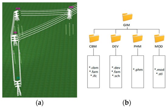
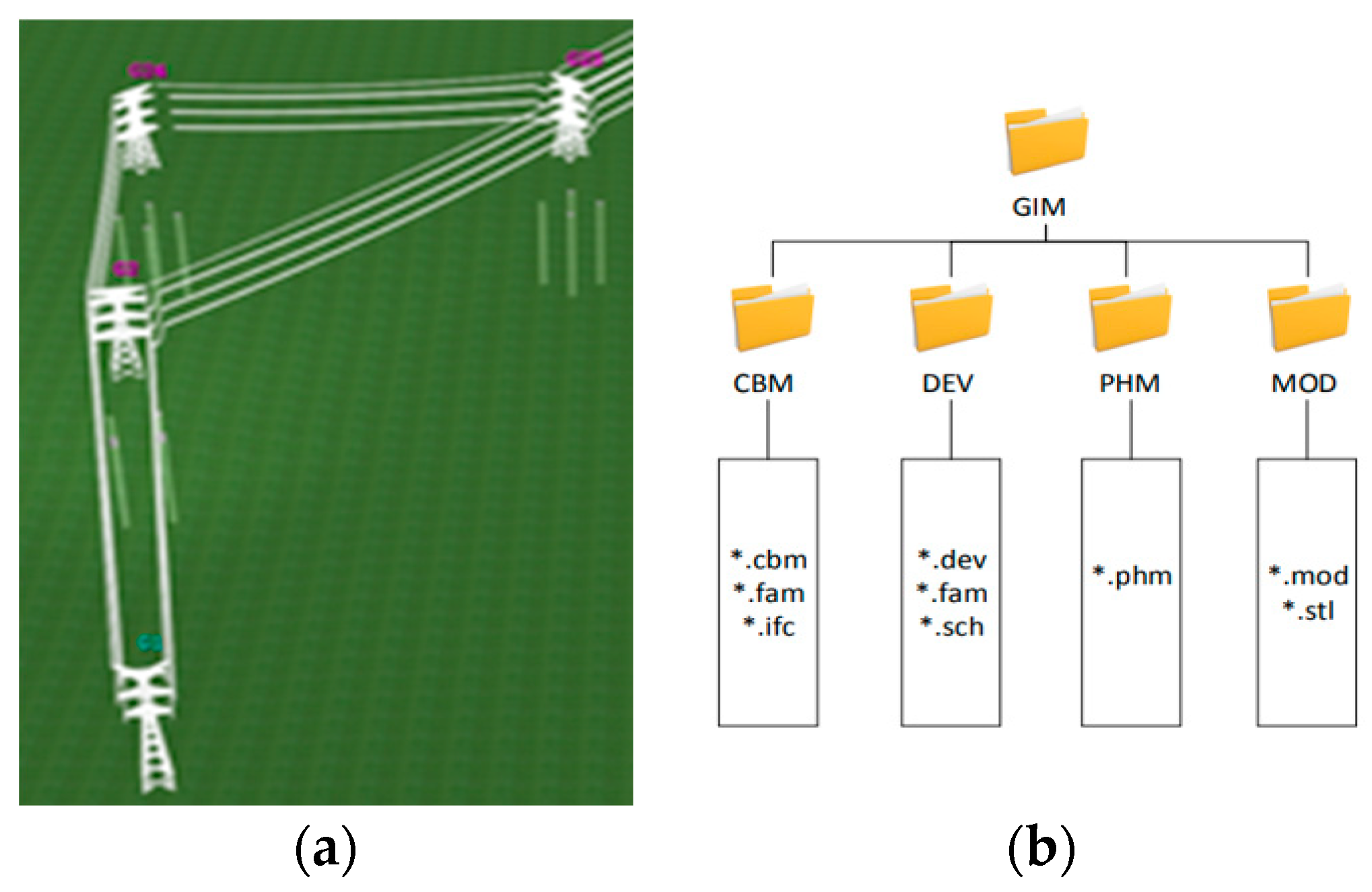
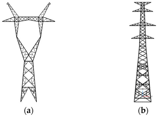
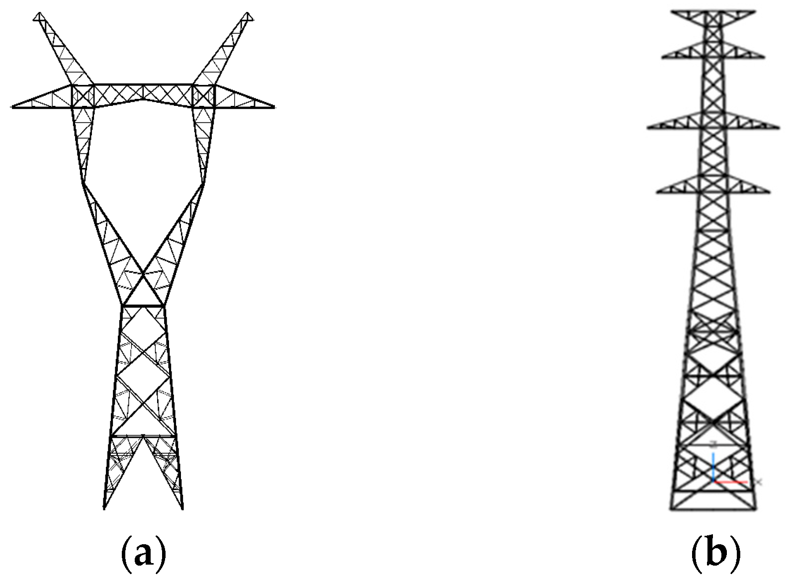
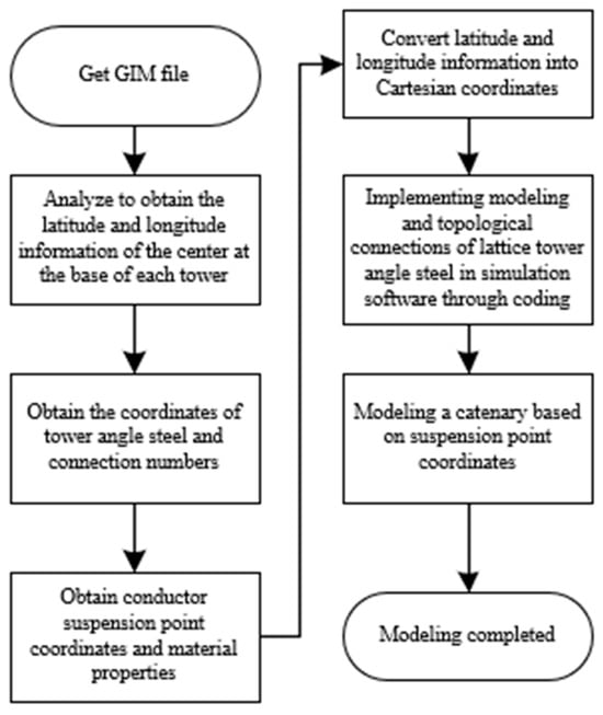
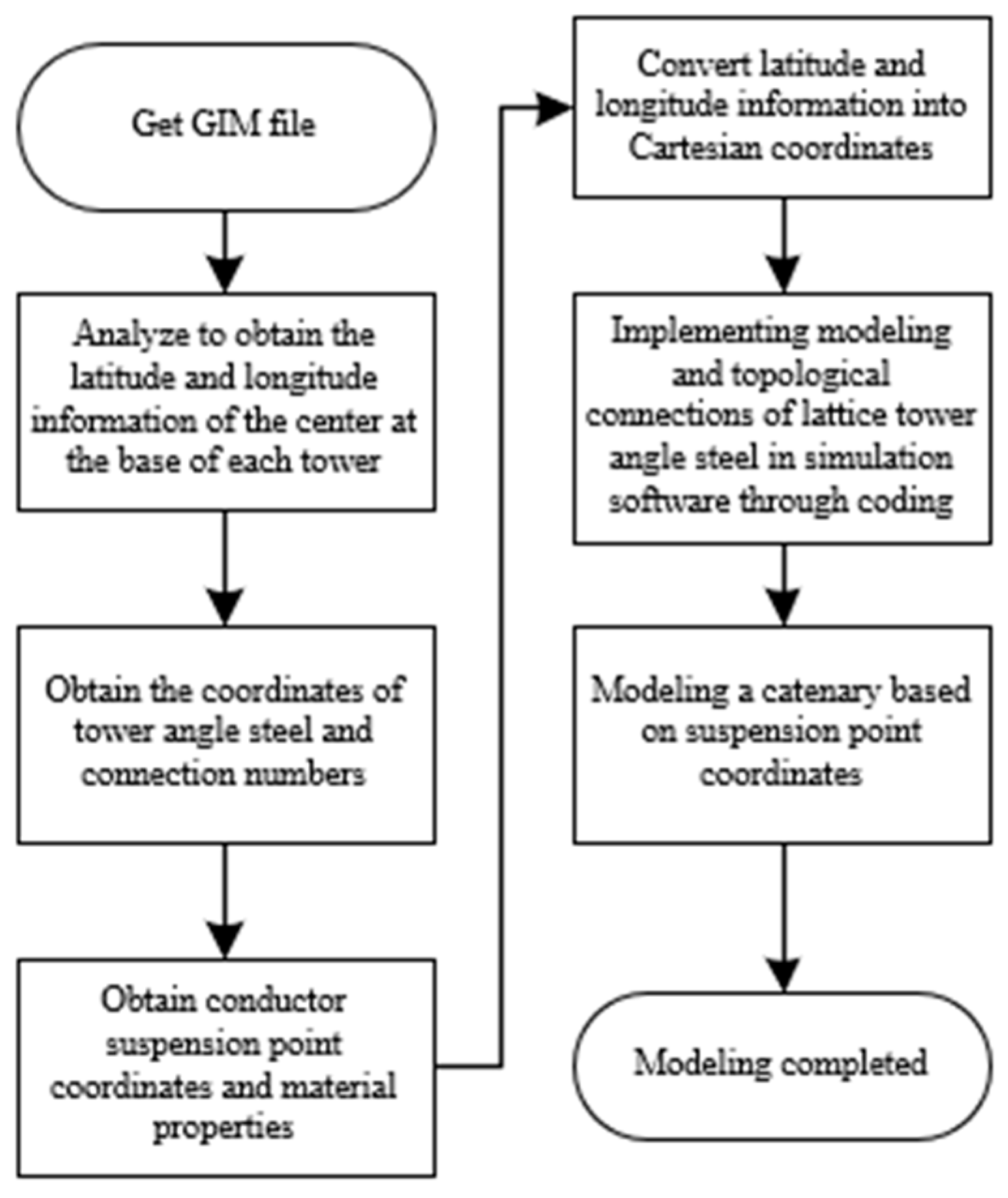
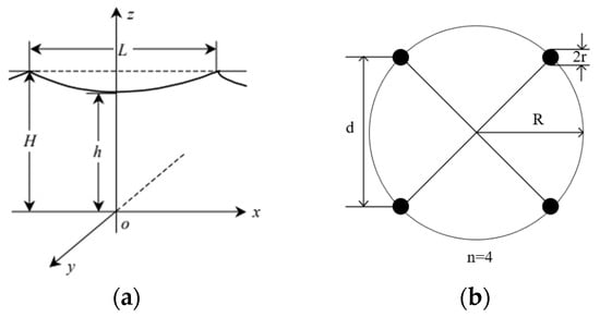
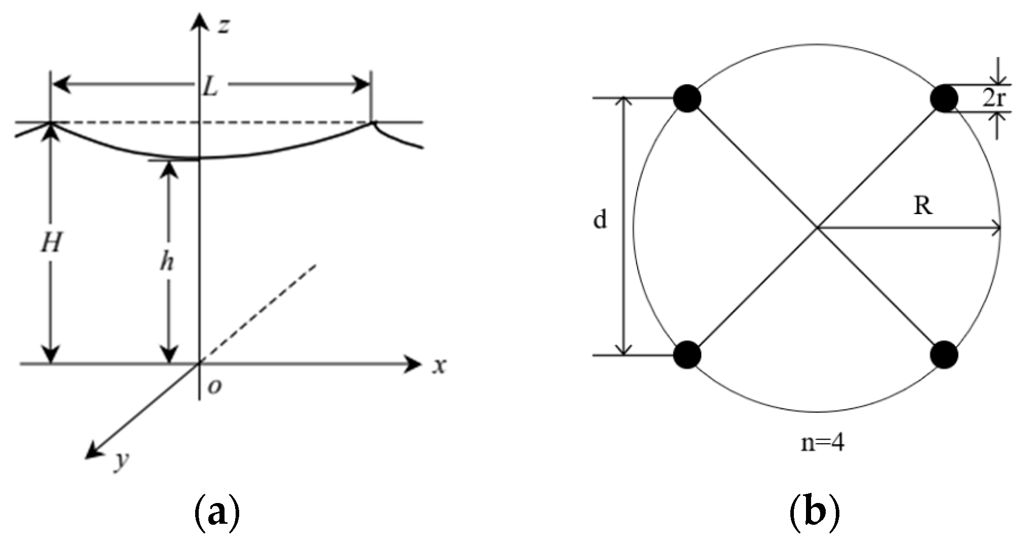
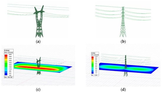
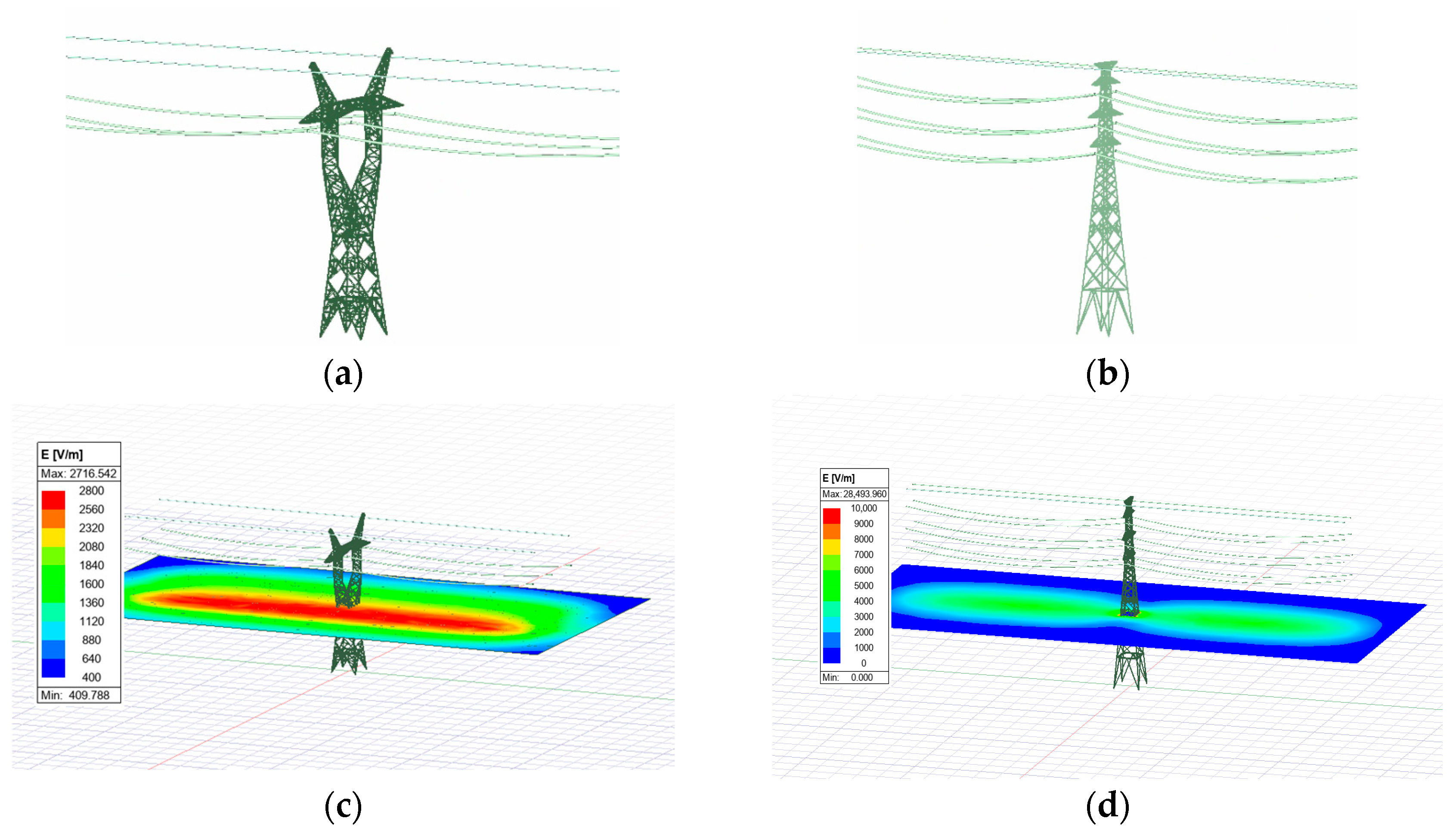
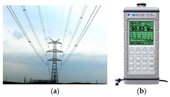
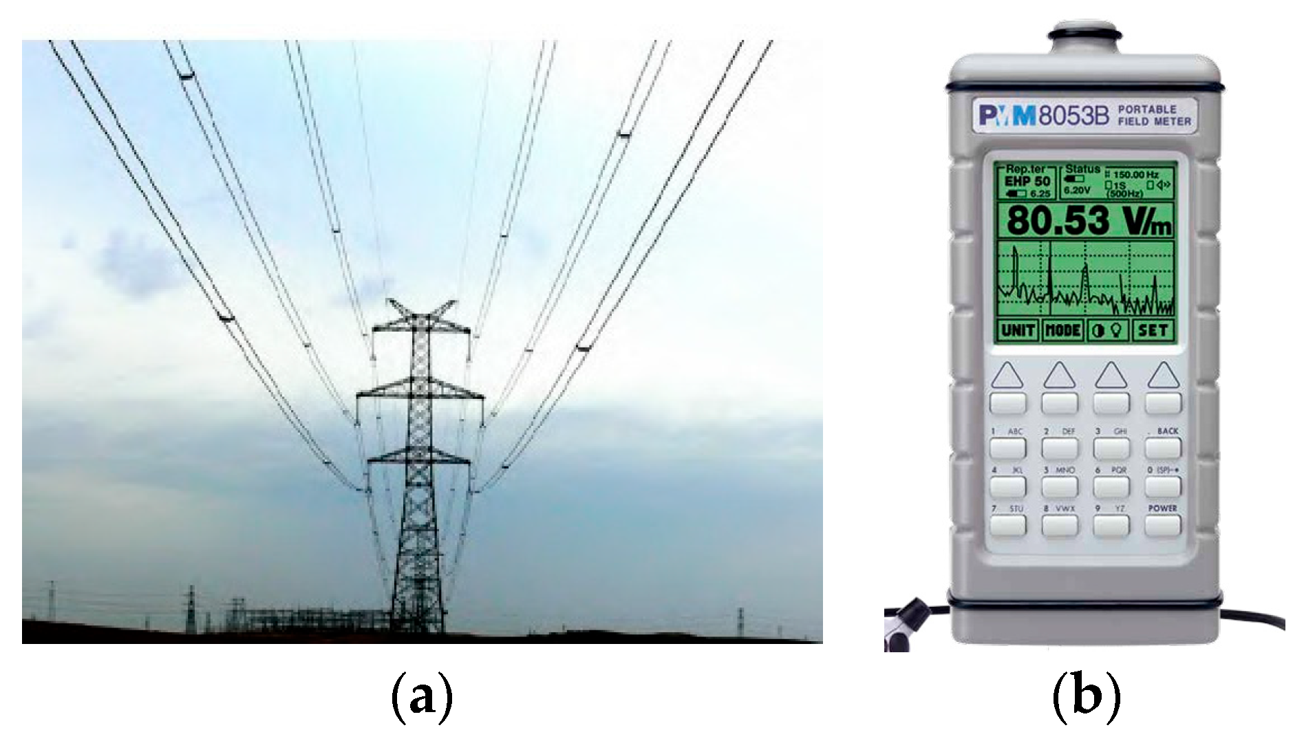
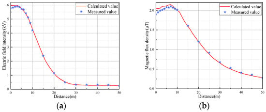
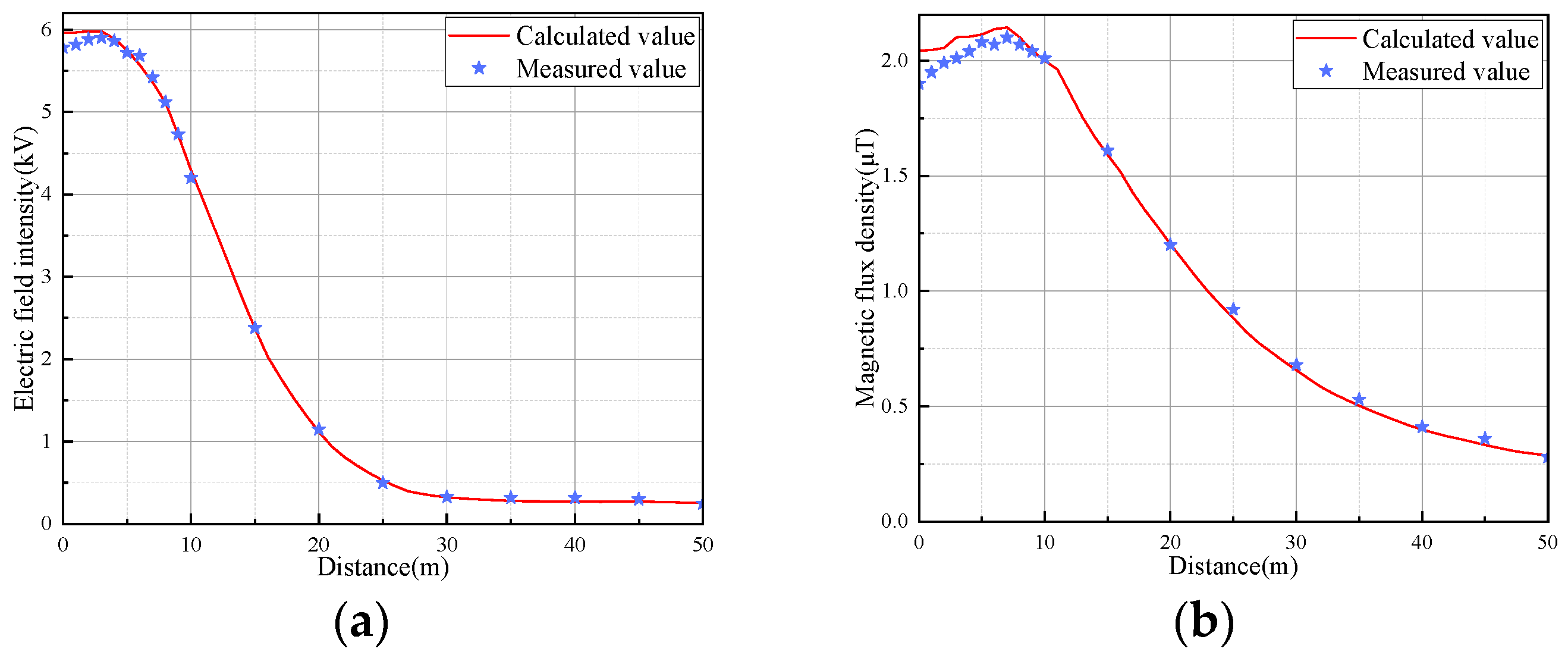
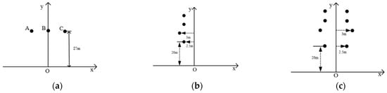
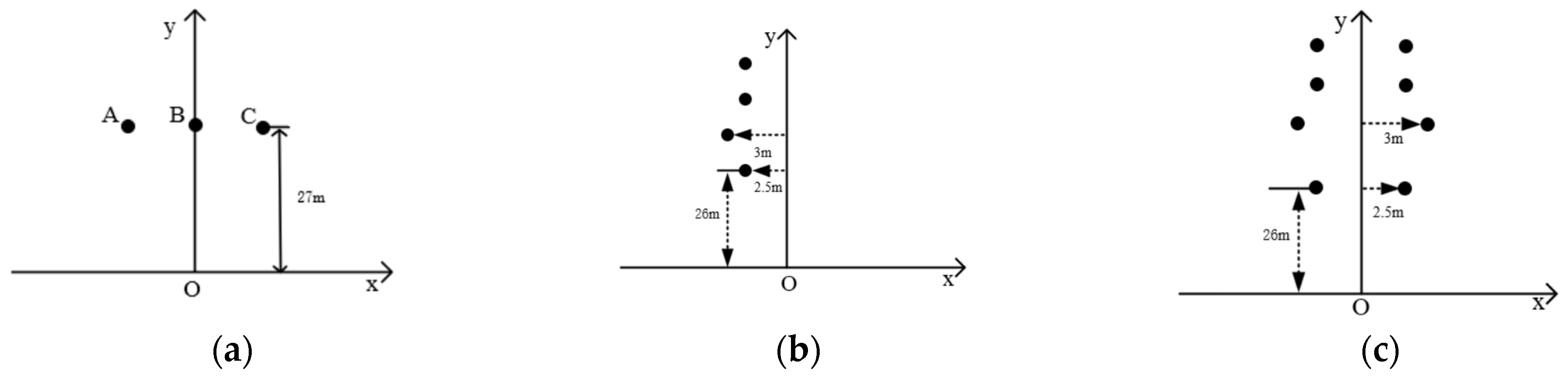
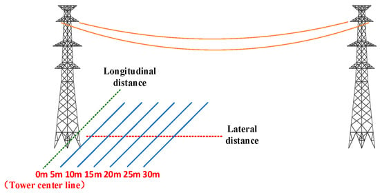
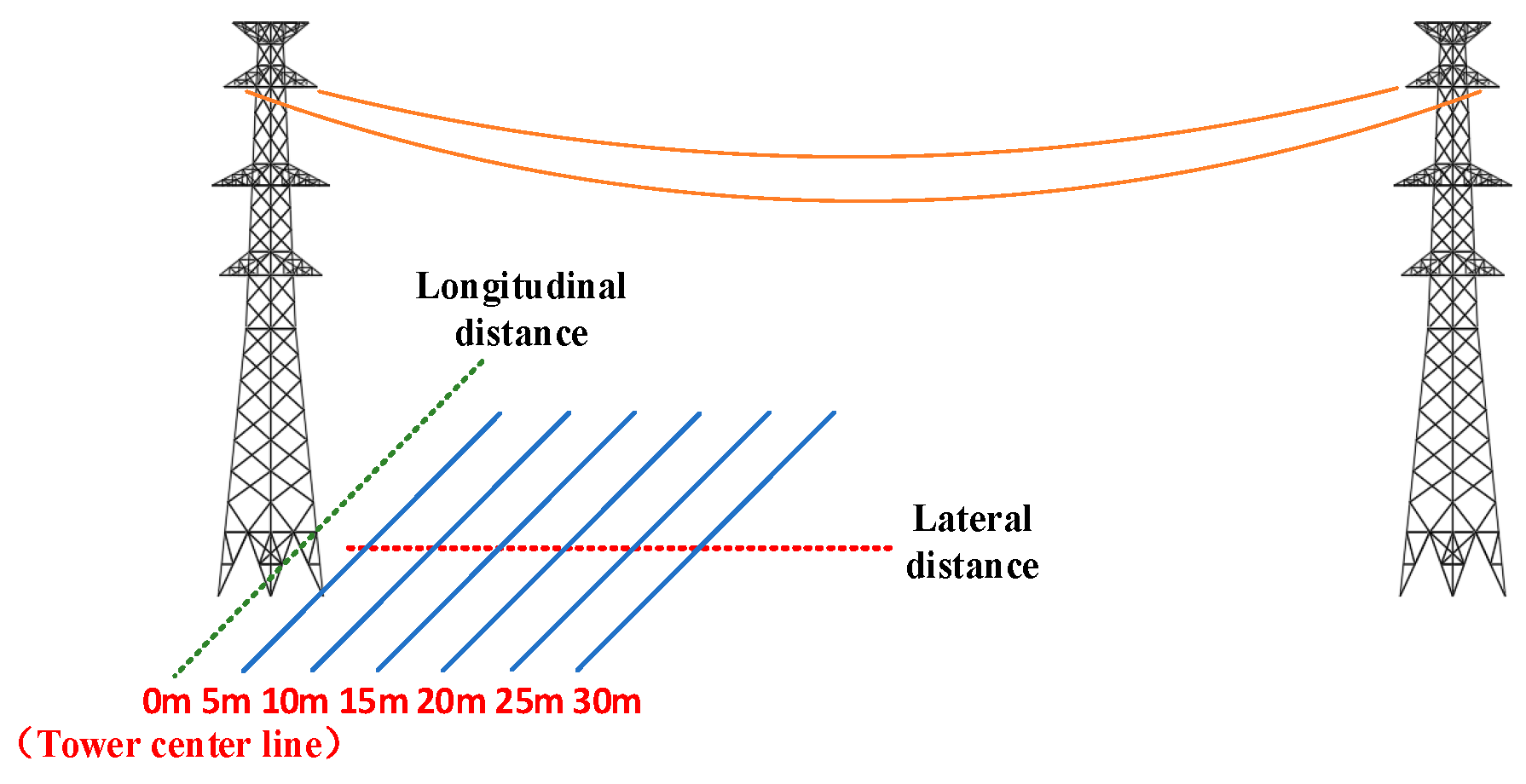
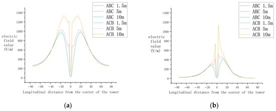
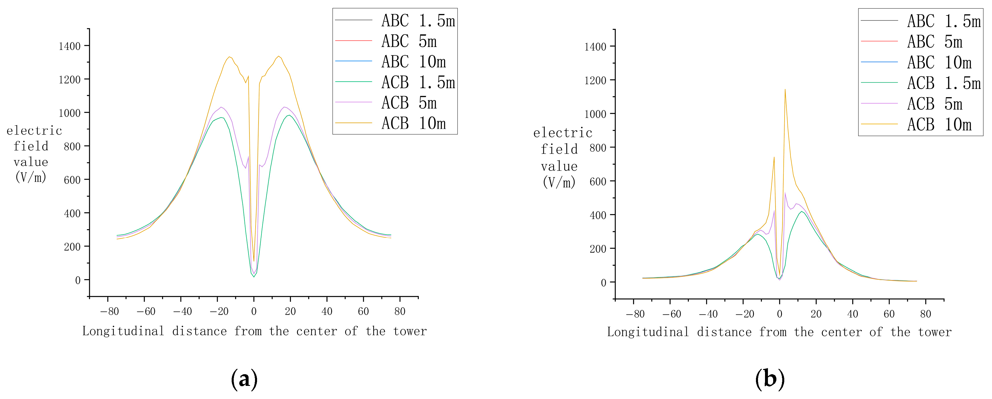
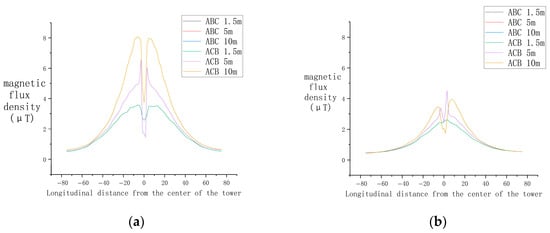
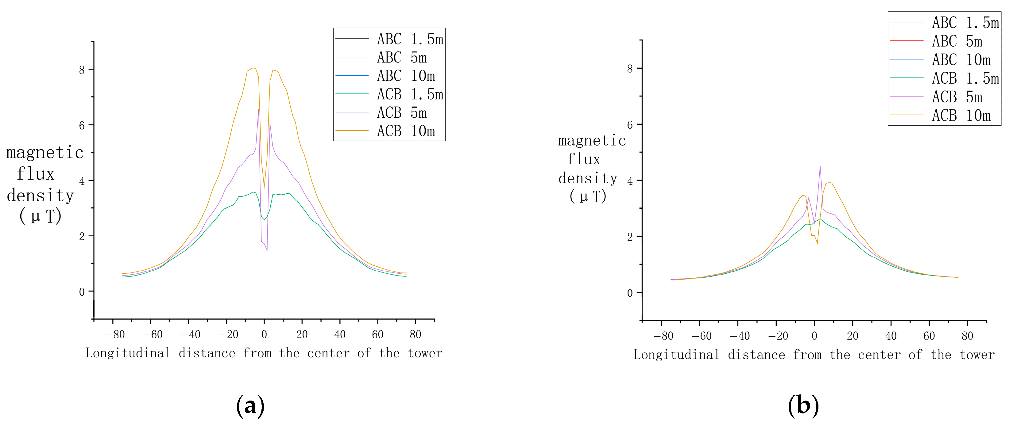
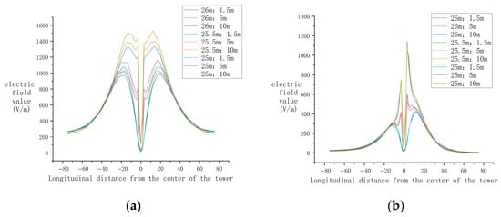
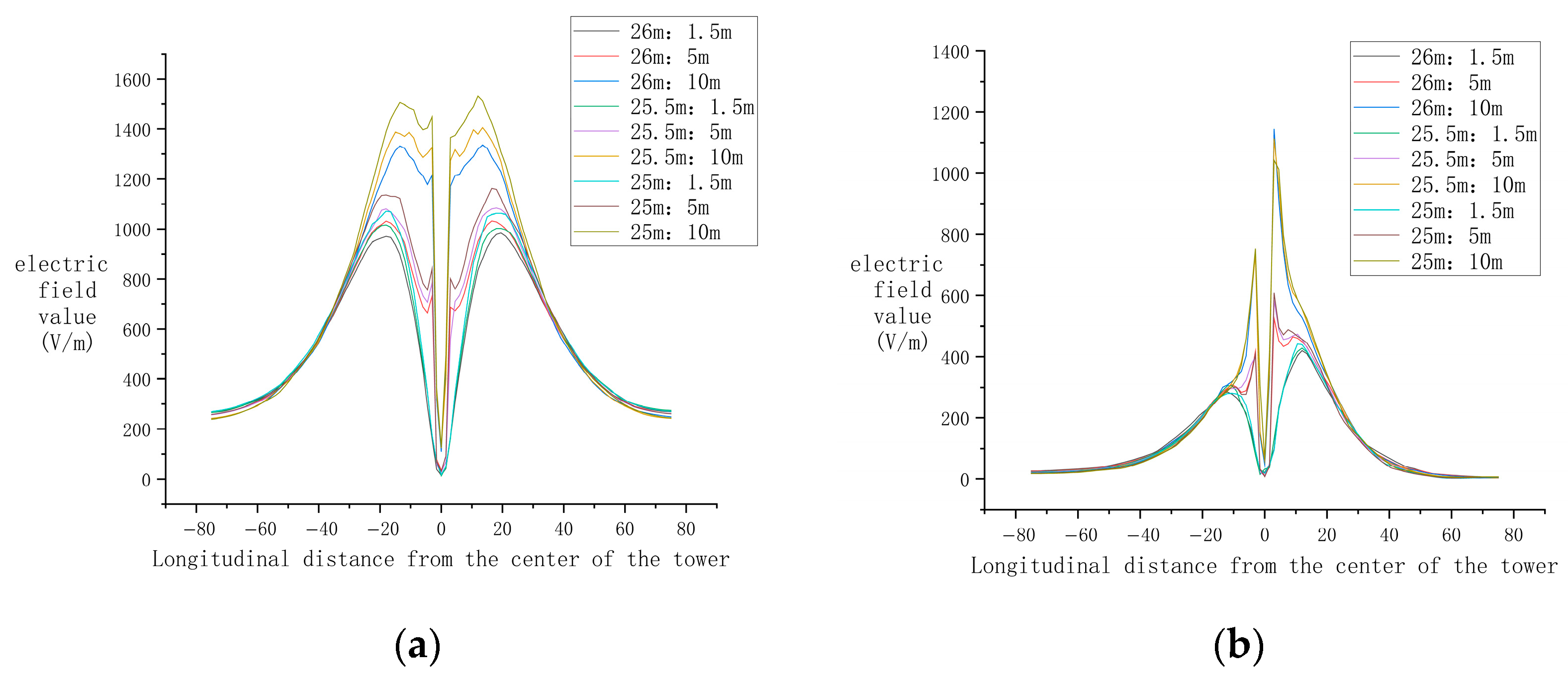
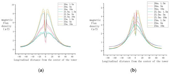
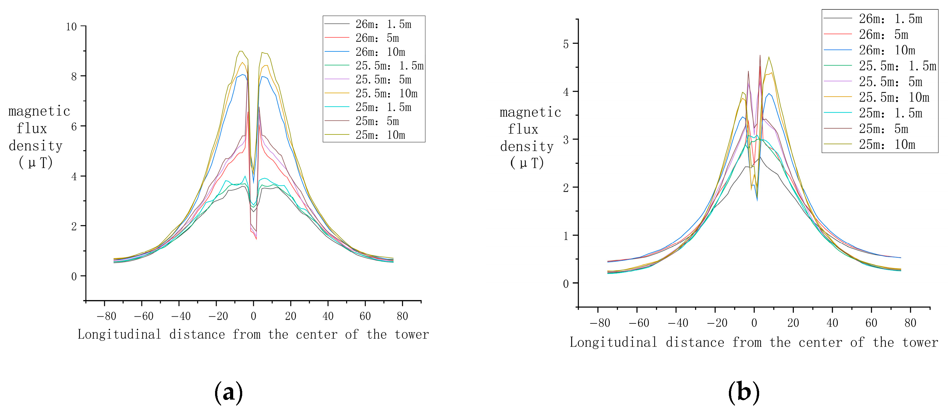
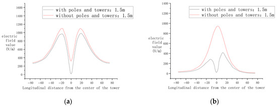
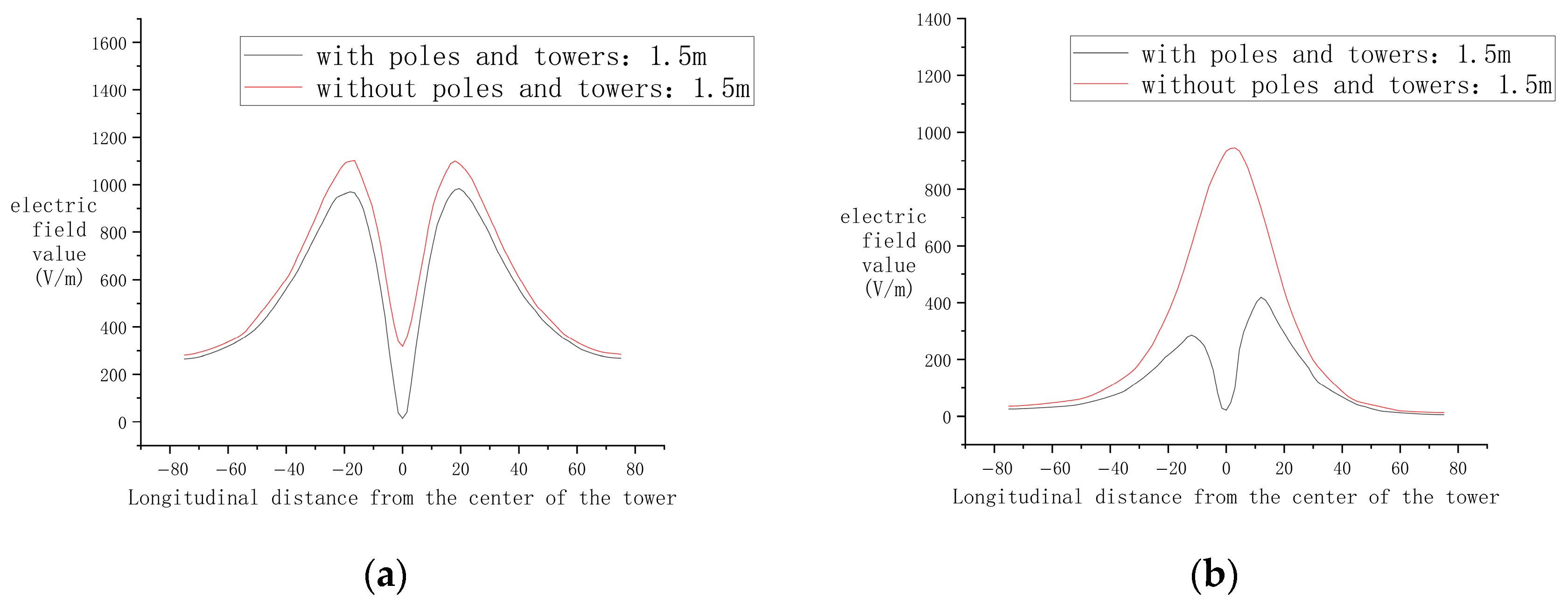
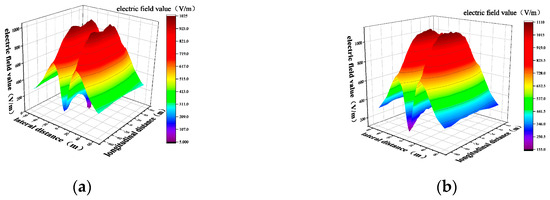
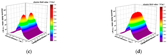
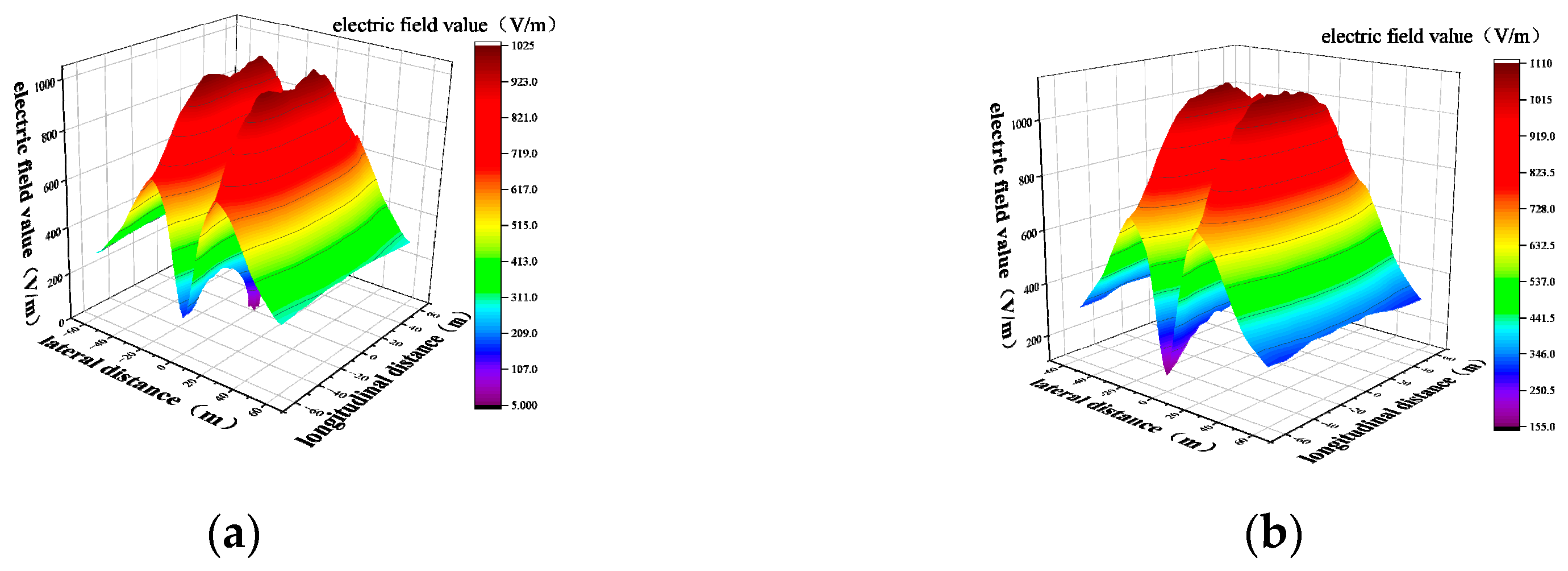
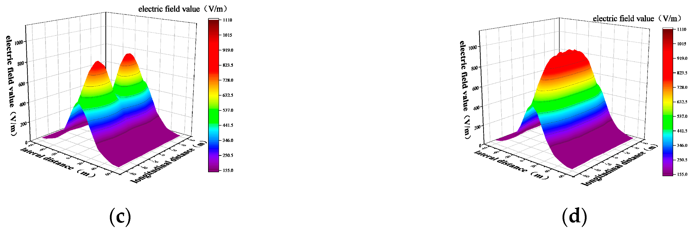
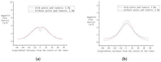
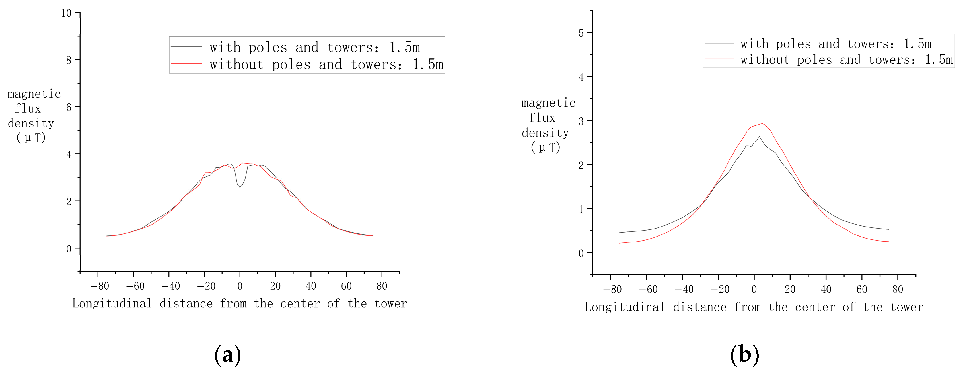
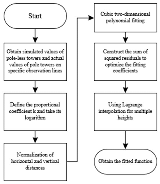
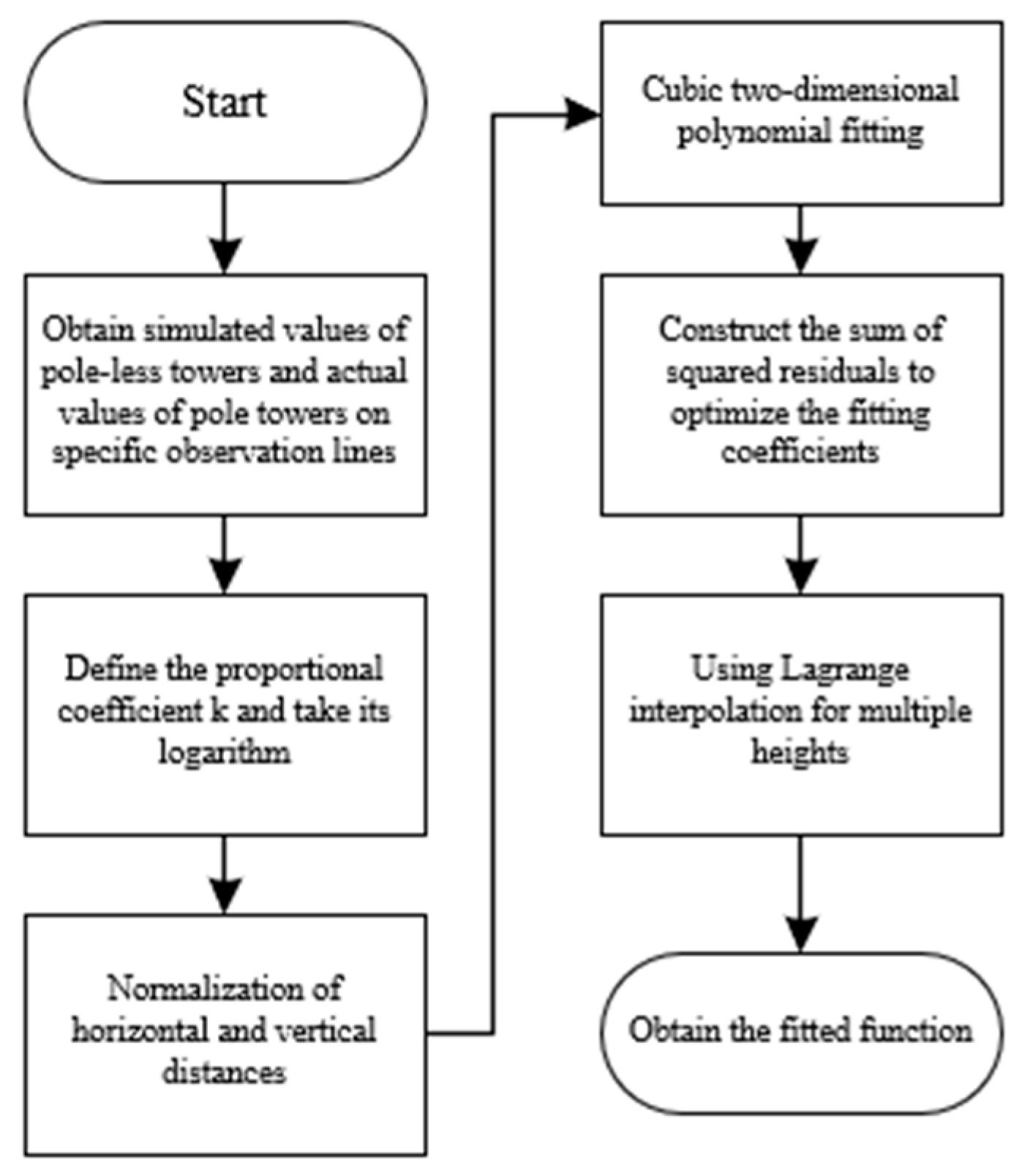
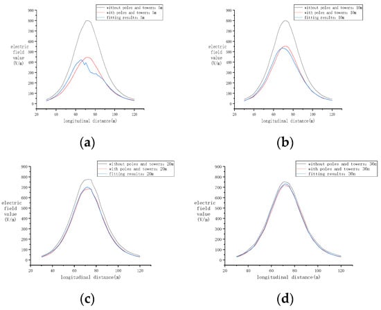
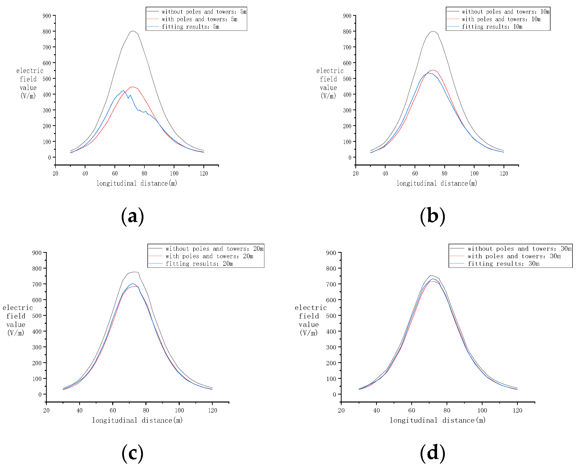
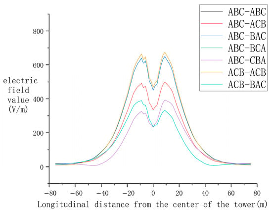
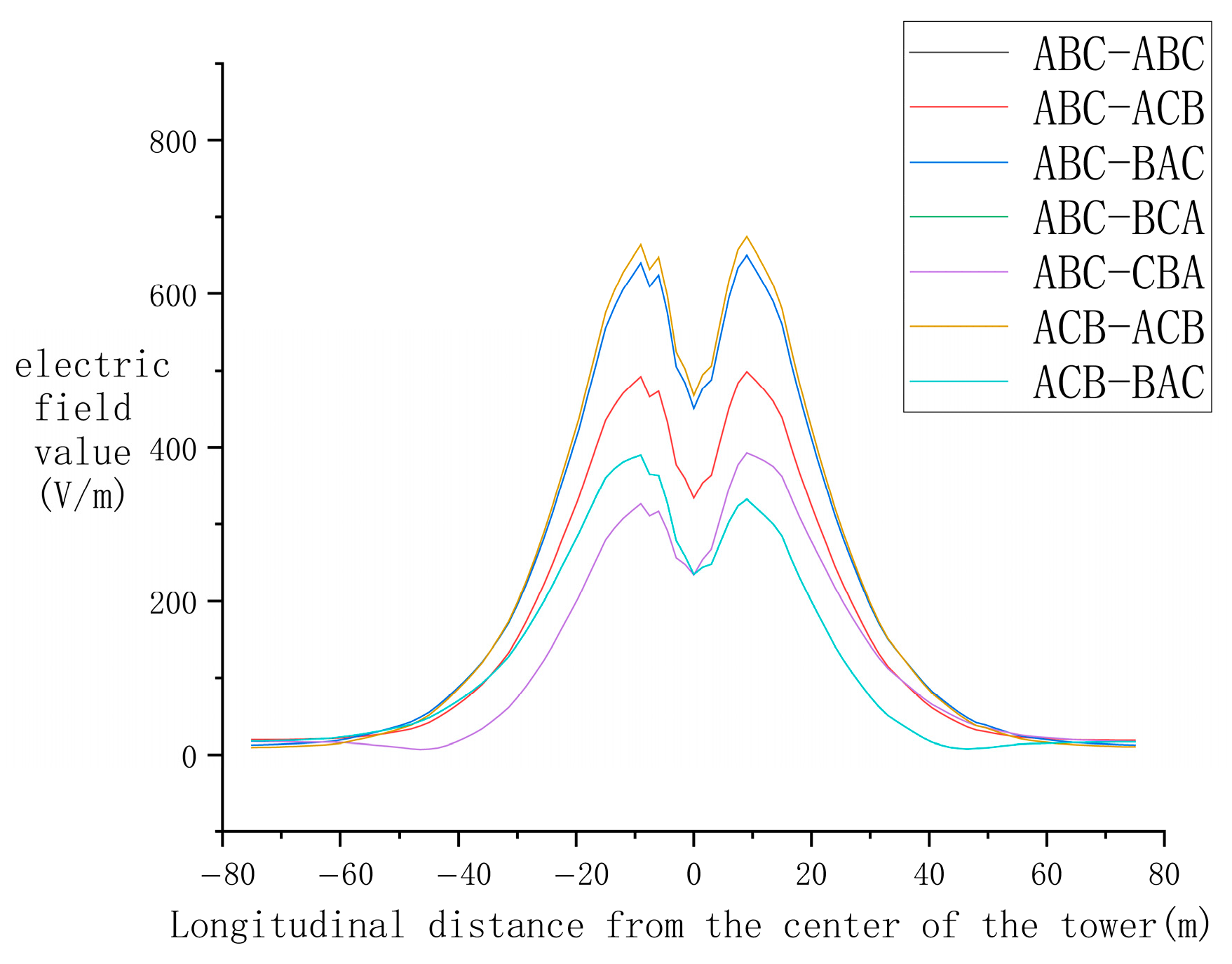
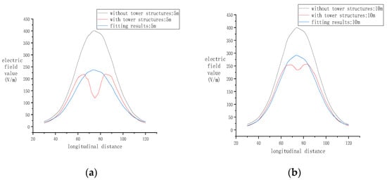
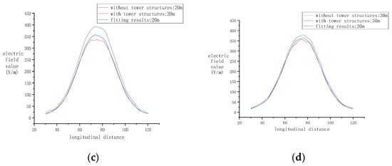
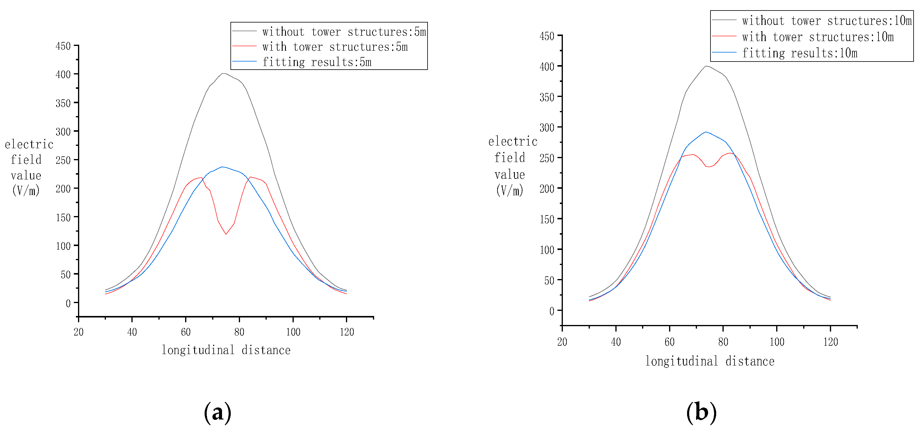
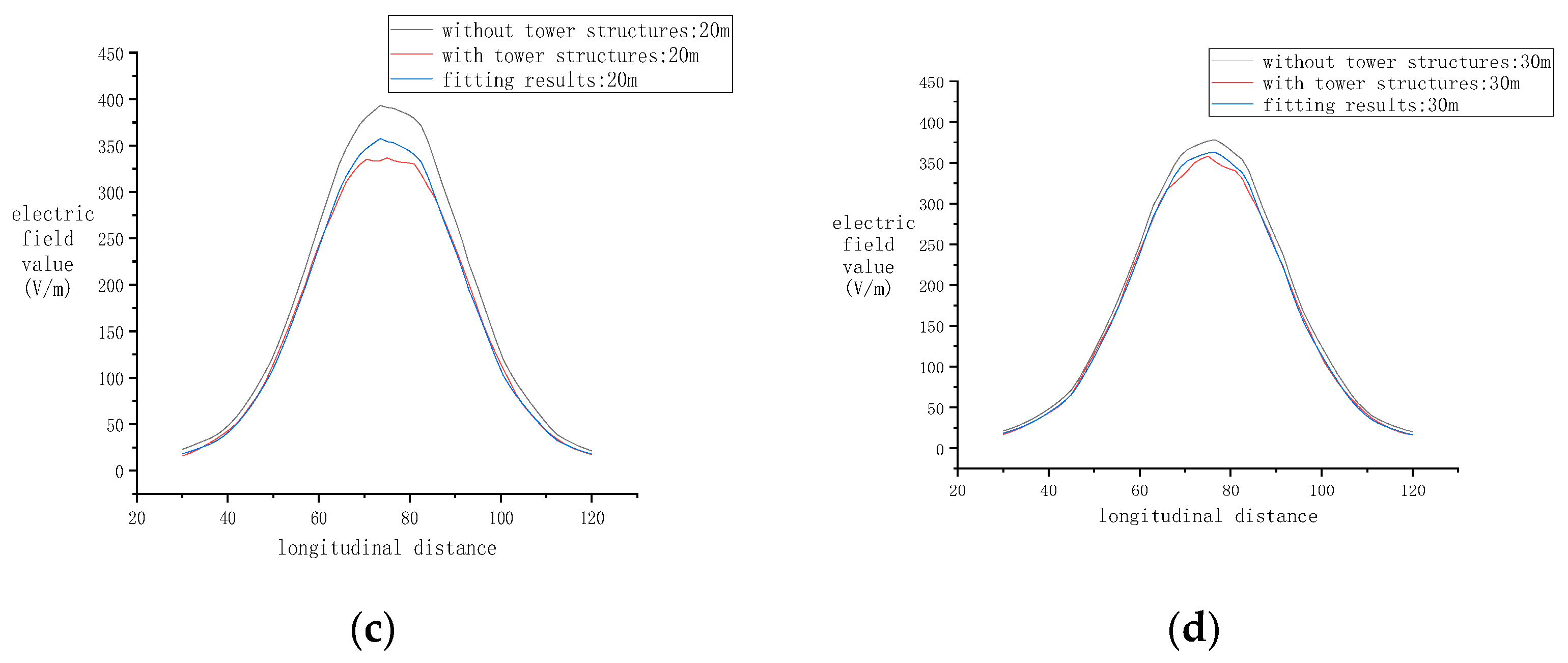
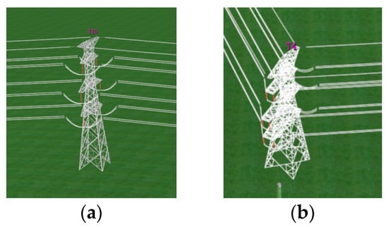
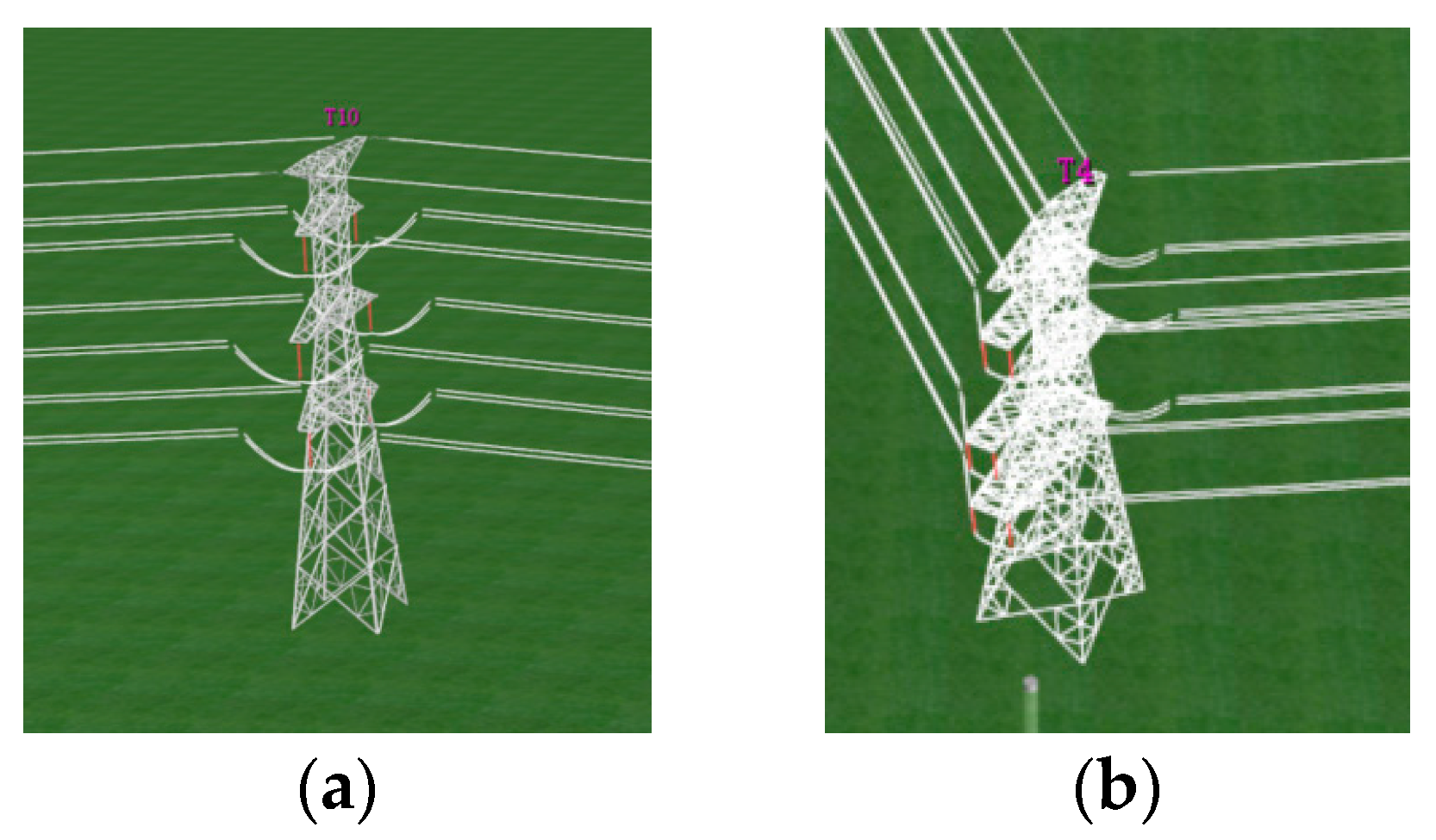
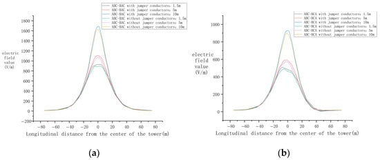
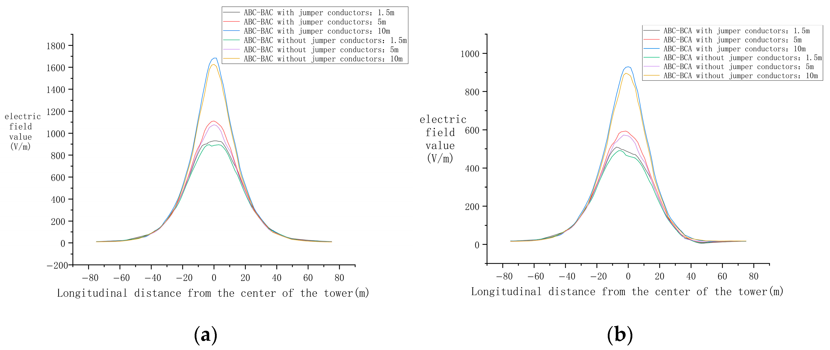
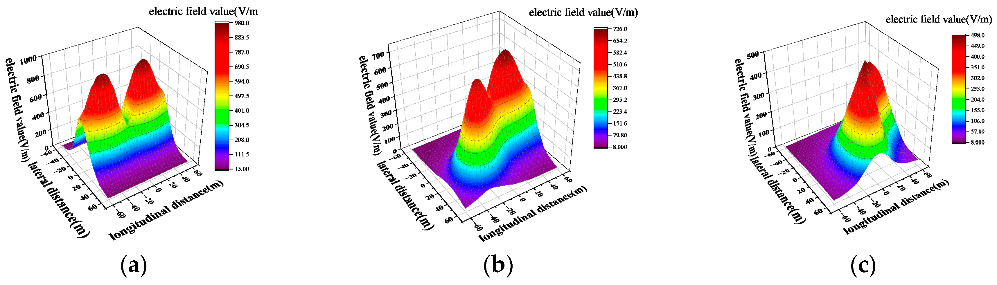
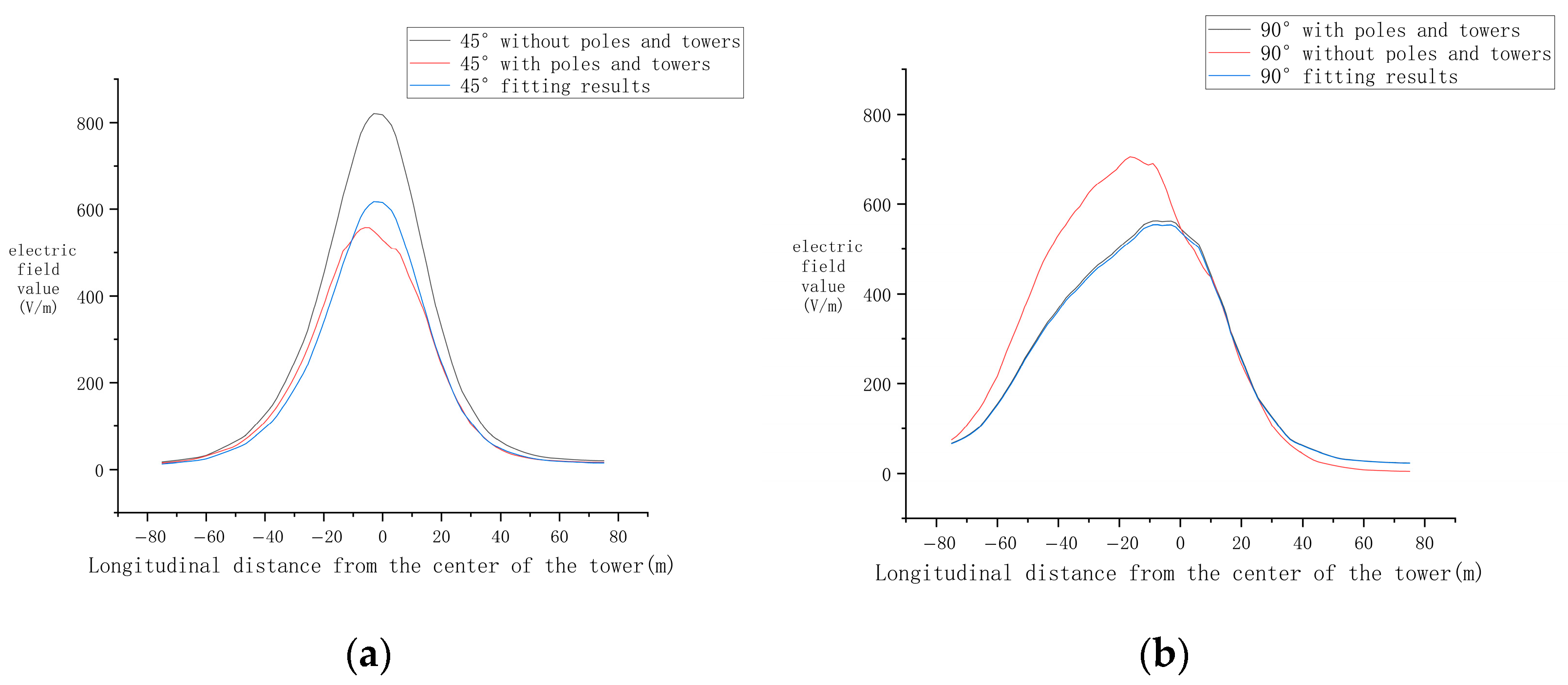

Disclaimer/Publisher’s Note: The statements, opinions and data contained in all publications are solely those of the individual author(s) and contributor(s) and not of MDPI and/or the editor(s). MDPI and/or the editor(s) disclaim responsibility for any injury to people or property resulting from any ideas, methods, instructions or products referred to in the content. |
© 2026 by the authors. Licensee MDPI, Basel, Switzerland. This article is an open access article distributed under the terms and conditions of the Creative Commons Attribution (CC BY) license.