


Abstract
In this paper, we provide a thorough review of novel machine learning (ML) models for anomalous sound detection (ASD). We focus on deploying models to highly constrained, embedded systems and tiny ML, and using single-channel sound as the data input. The survey includes only the works published in 2020 and later. Researchers address the anomaly detection task in various ways, borrowing models and techniques from such fields as speech processing, audio generation, and even computer vision. However, it is not clear which of these are suitable for embedded systems, meeting their constraints such as memory or compute. To address that, we provide a deep analysis of these models and optimization techniques applied to meet the design criteria for embedded platforms. We consider both deep learning and classical ML methods. We define categories for the anomaly detection methods depending on the approach taken to provide a structure and simplify the comparison of methods. We aim to provide a guideline on how to develop ASD systems and how to efficiently deploy the models on the embedded platforms.
1. Introduction
Anomalies are abnormalities, deviants or outliers, i.e., samples that do not fit the distribution [1]. In a more descriptive way, an anomaly can be characterized by means of (i) its scarcity, as anomalous/novel/outlier events occur less frequently than normalevents; (ii) its characteristics, as anomalous/novel/outlier events should have different characteristics than normal events; (iii) its meaning, as such events should carry a specific and different meaning than normal events [2]. A possible issue with this definition, though, is that the assumption about scarcity may yield a high rate of false positives. Various normal events may also occur less frequently. Second, the difference in characteristics may not necessarily be enough to decide whether a sample is indeed an outlier. An alternative definition of anomaly says that it is an event that cannot be explained with the normal model [3]. Despite the overlap, there are different definitions for seemingly the same phenomena. It is not trivial to define an anomaly as it depends on the system’s behavior. This also implies the need to evaluate how normal the sample is or, more commonly, to calculate its anomaly score.
Anomaly detection is therefore the task of finding unusual samples. In the unsupervised setting, we consider a training dataset that consists only of normal data samples, i.e., anomalous samples are not known in advance. Anomaly detection algorithms can be used in a wide range of applications, such as the quality inspection of products, equipment maintenance, network intrusion detection, or fraud detection. These algorithms are applied in the automotive, power, infrastructure, and financial industries. Early fault detection can prevent any serious damage to the equipment, stoppage of production lines, and financial losses.
Machine learning (ML) models are becoming commonly deployed to detect anomalies on the edge devices that constitute the Internet of Things (IoT). These tiny in size systems, despite a very low power budget are often equipped with accelerators and increasingly large computing resources. In parallel, significant improvements have been made in software and deep learning (DL) frameworks. Model optimization and deployment toolchains are available to bring these models, previously restricted to large systems, onto the embedded platforms. These can often be retrofitted to the existing industrial devices without impacting the operation of the monitored infrastructure. For instance, vibration sensors or microphones can be placed on the surface or in the vicinity of the monitored device.
In systems with microphones, the task is to determine if the sound emitted by an object is normal or anomalous [4]. The latter task is referred to as anomalous sound detection (ASD). The data is obtained using a microphone or an array of microphones. These sounds may have different characteristics, e.g., a spinning motor of a rotary moving machine generates harmonic, periodic noise. A fault may introduce additional harmonic distortions that can be observed continuously. Conversely, a valve or a slider follows a rectilinear movement. Similarly, a loud noise in the outdoor environment, e.g., a car crash, is instantaneous and often very brief. Hence, anomalies should be detectable even from a single or only several occurrences. In practice, operational states of a machine or environmental noise can change and cause domain shifts. Over time, what was deemed a normal sample can become an anomaly, and conversely, an anomalous state can become the new normal. Therefore, models should be capable of addressing the domain shift, i.e., non-stationarity of the monitored process. There is a growing need to develop early warning systems where the response time is critical. Tasks for such systems are becoming more complex, whereby models that address them are gaining in complexity. Running the models on edge devices is essential to achieve fast response times and good accuracy. It is actually the setting that is the focus of this work, i.e., using embedded, highly constrained systems for ASD on the running equipment. We task ourselves with conducting a thorough survey of ML models and methods for ASD, and then evaluating their suitability for edge systems. We focus exclusively on acoustic data to provide a more thorough analysis of models and methods employed in ASD. The setting is predominantly the single-channel ASD, although we believe many of the findings may apply to the multi-channel ASD as well. We note that applications often utilize other modalities, e.g., vibration, temperature, in conjunction with acoustic data. We hope that this work may serve as a guide for researchers and developers to help them understand modern ASD. This paper serves as an extension of our submission on comparison of methods for anomaly detection on edge systems [5].
The paper is structured as follows. Section 2 summarizes the related surveys. In Section 3, we provide research questions (RQs) we aim to answer and the methodology used to collect and analyze the articles. Section 4 summarizes the results of the survey. Section 5, Section 6 and Section 7 provide detailed information on the techniques and models used in ASD, i.e., audio feature processing, modeling, and anomaly scoring, respectively. Section 8 deals with design criteria and constraints for model deployment on embedded systems. Section 9 analyzes ASD techniques in the context of embedded systems and their constraints to formulate the design guidelines for edge ASD systems. We provide the guidelines for researchers and developers in the field of ASD in Section 10.
2. Related Works
Prior to conducting our survey, we analyzed review papers that deal with anomaly detection using sound and general anomaly detection on embedded or IoT systems. We focus primarily on the questions and problems that other surveys answer and their references that may be helpful for the readers. Lastly, analyzing other publications helps formalize the data extraction protocol for our survey, i.e., which key aspects to include when making a comparison of the published papers.
The general summary is presented in Table 1. One can identify that we were not able to find a survey that covers ASD on embedded systems. The surveys dealing with anomalies on IoT refer to microprocessor (MPU) systems, e.g., Rapsberry PIs, and rarely deal with tiny edge platforms, which are the focus of this work. General ASD is a well-studied area discussed in various works. However, many models or approaches are not applicable to edge systems due to their memory or computational requirements. With advancements in models and with increasing availability of more powerful hardware, we identify the need for a survey that (i) deals with ASD, (ii) addresses edge platforms and identifies the constraints, (iii) provides reference ASD methods that may be deployed on highly constrained edge systems.
Table 1.
Comparison of anomaly detection surveys in terms of focus areas. A dash (−) indicates that the given area was not covered in the survey, while a checkmark (✓) indicates that the area was covered in a dedicated paragraph or section.
In [6], Mnasri et al. provide a comprehensive survey of anomalous sound event detection (SED), covering feature extraction methods, applications, and evaluation metrics. The datasets for SED are discussed. The open problems in anomaly detection are also described with reference to the published works and the potential solutions. This survey does not deal with either computational complexity or the embedded domain.
In their work, DeMedeiros et al. review anomaly detection techniques used in IoT and sensor networks [8]. The authors propose distinguishing between point-based (events), collective (window with multiple events), and continuous anomalies. This survey deals with various applications and settings, including a malicious actor, sensor performance, and time-series data. However, the datasets and papers analyzed do not address ASD. Among the surveyed papers, only 3 out of 32 adopt approaches other than DL.
Railway anomaly detection using both audio and video data with DL is surveyed by De Donato et al. [7]. They evaluate the models and datasets used for anomaly detection and outline the current, open challenges. The authors identify that audio signals are utilized only in a limited way for anomaly detection in railway systems (5 papers out of 95 surveyed), whereas not even one system supports multi-modality.
Siliang et al. provide a high-level survey of IoT-based methods and applications for fault diagnosis [10]. Authors discuss latency, resource consumption, privacy, and scalability. The model complexity and optimization for the edge are also described. The emphasis is on MPU-based systems with 2, 4, or more cores, with only a single example of a more constrained microcontroller (MCU).
Darban et al. [9] work is focused on anomaly detection using time-series data with DL. They provide a detailed description of the system architectures and datasets. The models under consideration include Recurrent Neural Network (RNN), Convolutional Neural Network (CNN), Autoencoder (AE), Variational Autoencoder (VAE), Hierarchical Temporal Memory (HTM) [13], and transformers, among others. The authors classify each model based on the input types, interpretability, or learning type (e.g., supervised). They describe a large number of datasets for anomaly-detection applications, which include medical, aerospace, industrial, and urban events.
IoT anomaly detection with time-series data is also discussed by Sgueglia et al. [11]. The authors review 62 papers published from 2014 to 2021 and discuss dimensionality reduction and feature extraction, real-time monitoring, and datasets. They also provide a detailed overview of embedded-system constraints (latency or power) and anomaly types. This is followed by a discussion on ML and DL methods for anomaly detection.
In [12], Gairí et al. present a review of environmental sound recognition (ESR) methods designed for embedded and resource-constrained devices. The authors analyze deep learning approaches for audio classification with emphasis on deployment on microcontrollers, edge devices, and low-power platforms. The survey discusses feature extraction techniques, neural network architectures such as CNNs, RNNs, and lightweight models, as well as optimization methods including quantization, pruning, and model compression to meet memory and latency constraints. In contrast to general ESR surveys, this work explicitly considers hardware limitations and real-time requirements, providing a comparison of existing implementations on embedded platforms. However, the review focuses on general sound classification rather than anomaly detection, and therefore does not analyze ASD-specific datasets, evaluation protocols, or detection-oriented model designs.
3. Methodology
The key RQs we aim to answer are as follows:
- RQ1: What models and techniques are used for ASD?
- RQ2: What are the criteria and constraints to consider when deploying models on embedded systems?
- RQ3: Which models and techniques for anomaly detection using sound are suitable for embedded systems?
We apply systematic review methodology [14,15] to design and prepare the survey. We research IEEE Xplore and ACM libraries, proceedings of NIPS, ICLR, ICML conferences, as well as DCASE workshops Task 2 (anomaly detection using sound). We limit the types of works to papers written in English, published in journals or at conferences, and technical reports of DCASE workshops. We limit our search to the works published in 2020 and later. Then, we define keywords for each of the subdomains found in RQs as follows:
- 1.
- Anomaly detection: anomaly, defect, fault detection, outlier, out-of-distribution.
- 2.
- Sound: sound, acoustic, microphone, audio.
- 3.
- Embedded systems: embedded, tiny, edge, internet-of-things, iot.
For RQ1 we use sets (1) and (2), and for RQ2 we use set (3). To answer RQ3, we use the results extracted from RQ1 and RQ2, as presented in Figure 1. The search query uses OR among the keywords in a specific subdomain, as well as the logic operator AND between the sets. We use wildcards to broaden the search and variations of the key terms (Internet-of-Things as well as Internet of Things). The keywords are searched for in metadata, including the paper title, abstract, and its keywords. Note that we do not limit the search to DL or even more broadly to ML. For IEEE and ACM, we use advanced search tools. We also remove works focusing on anomalies in access control from the networking perspective (intrusion detection) or anomalies of the embedded system itself. We filter out reviews and surveys, non-experimental works, applications of hardware platforms developed before 2020, or hardware that is not considered an embedded system (e.g., servers in base stations), and the edge of data centers (also referred to as edge systems). For NIPS, ICLR, and ICML conferences, we perform a manual search. That is, we search for any mentioned term in the titles or abstracts of the published articles. Then, we subjectively analyze the selected abstracts for relevance to ASD or anomaly detection on edge systems. For DCASE, we initially selected all the technical reports submitted for Task 2, which is unsupervised detection of anomalous sound for machine condition monitoring [4]. The task is expanded on a yearly basis with new difficulties introduced (out-of-domain data, first-shot learning). For each technical report, we search for the conference or journal article. If available, we use it instead of the technical report.
Figure 1.
Survey methodology and RQs it aims to answer.
In IEEE and ACM sources, we analyze titles, abstracts, citations, and contents to filter out papers not related to this survey (for instance, acoustic source localization), without empirical results and other surveys. For RQ2, as we aim to obtain information about models deployed on embedded devices, we filter out papers explicitly mentioning running models in the cloud with data sent from IoT nodes.
For RQ1, a total of 192 published works are selected. These are analyzed to extract the required information, including the models used, pre-processing, and data augmentation. We also evaluate the papers in terms of the quality, clarity, and overall fit with the survey subject. We note that the paper’s evaluation introduces subjective researcher bias, and to reduce the risk of this bias during the literature screening process, the abstract and full-text review stages were conducted jointly by all authors of this manuscript. Each paper was evaluated independently by multiple authors, and disagreements regarding inclusion or exclusion were resolved through discussion until consensus was reached. We finally select 103 papers to answer RQ1, with 82 papers being technical reports originating from the DCASE challenges. Out of these 82, we have found 27 conference or journal papers based on the technical report.
For RQ2, we browse NIPS, ICLR, and ICML proceedings to find relevant works. While existing surveys identify several limitations regarding the deployment of models on edge devices [16,17,18], these findings require validation and revision. We originally selected 19 articles that were highly likely to have been disregarded in the above surveys due to their publication date or subject matter. After the initial read, we chose 12 papers to compile the list of constraints for the embedded systems. These works discuss the constraints and optimization techniques used to address them during implementation on the embedded systems. All the selected papers were referenced in Section 8.
In RQ3, we combine the results of RQ1 (i.e., audio features, models, and anomaly scoring techniques) and evaluate them in terms of the constraints defined in RQ2. We search for papers presenting a technique or a model employed on an embedded system such as an MCU, a field-programmable gate array (FPGA), an application-specific integrated circuit (ASIC), or a digital signal processor (DSP). We provide references to the implementations and, if no papers are found for a technique, we label them as not found. We also provide references to the software and hardware platforms that meet the requirements of RQ2 and allow for the deployment of models found in RQ1. We then provide the guidelines on how to deploy and run models from a complete workflow point of view.
4. Results
In the surveyed ASD papers, the researchers in almost every case build a processing pipeline (see Figure 2). The inputs are raw audio recordings preprocessed into higher-level audio features. During training, data augmentation is often applied. Then, the anomaly detection model is trained on the audio features. Once the data has been processed by the model, the outputs are evaluated using an anomaly scoring function. This final score is compared with the threshold to classify the input as either anomalous or normal.
Figure 2.
ASD model training and inference pipelines with sections detailing each step and selected examples. Training takes place in the cloud or on a workstation, using audio recordings. During training, data is preprocessed into audio features used to train the ML model and then the anomaly scoring model. Once training is completed, the model is optimized and converted to be deployed on the MCU. Inference and anomaly scoring are performed on the edge with live data from microphones.
The methods employed at each step vary significantly. We note that, as a large proportion of the surveyed papers originated from the DCASE challenge, they may be biased by baseline models. These models are proposed by the organizers and produce acceptable results for the given task. The nature of the challenge means that researchers, both with the improved results over the baseline and those not being able to surpass it, have to submit technical reports to be included in the list of attendees.
In real-world ASD systems, audio data is recorded by microphones and processed live. During research and model training, audio recordings are usually used. Each recording may be split into frames, which can be processed individually or, as in the DCASE challenge, several frames are concatenated together with a sliding window. Each window is processed from raw waveforms into high-level audio features. Then, the sliding window moves and selects the next batch of frames, usually with some overlap. This continues until all the frames in the recordings have been processed.
The most commonly used audio feature is the log mel spectrogram, followed by linear spectrograms, AudioSet feature extractor [19], and Mel-Frequency Cepstral Coefficients (MFCCs). We provide more details on audio features pre-processing and data augmentation in Section 5.
The next steps depend largely on how the ASD task is formulated:
- 1.
- Reconstruction-based—AEs or generative models are trained to minimize the mean squared reconstruction error of the given input data and the output of the model. The idea is that a model trained on normal samples is not able to reconstruct anomalies correctly. The higher the reconstruction error, the greater the anomaly score (see Figure 3).Figure 3. Conceptual illustration of anomaly detection with reconstruction-based task formulation using AE. Reconstruction error, calculated as difference between original x and reconstructed data sample, is used as anomaly score. The colormap ranges from dark purple (representing lower numerical values or background) to yellow (representing higher numerical values or distinct features). In the network architecture diagram, light blue blocks represent the input and output vectors, while darker blue blocks denote the hidden layers and the central latent space z.
- 2.
- Classification—a binary classifier is trained to distinguish normal samples from artificial anomalous ones, or a multiclass classifier is trained on the dataset obtained from, e.g., many running machines or device classes. In the latter case, the model is then deployed to monitor a known class of devices. If the samples are normal, the model should yield high confidence for this class. If any sample is anomalous, the confidence should be low, and the negative log likelihood for the correct class is used as the anomaly score. See Figure 4 and Figure 5 for binary and multiclass examples.Figure 4. Conceptual illustration of anomaly detection as binary classification using normal samples and synthetic samples to represent anomalies. Dark purple colors are representing lower numerical values and yellow color is representing higher numerical values.Figure 5. Conceptual illustration of anomaly detection as multiclass classification. Dark purple colors are representing lower numerical values and yellow color is representing higher numerical values. The model is trained with normal samples from multiple classes with class identifiers from 0 to 3. During the test, it is known that the model is running on device class 1. Given a normal sample of this class, confidence is high. When given a sample from any other class, model confidence is low, indicating an anomaly.
- 3.
- Embedding-based—a feature extraction model or a dimensionality reduction technique is used to transform the input audio features into a lower-dimensional representation, embeddings or feature vectors. The model can be trained to minimize the distance metric between normal samples while maximizing the distance for abnormal samples or those belonging to other classes [20]. The distance metric is usually the cosine distance. Alternatively, probability distributions or a separating decision boundary are learned on the embeddings of normal samples. The anomaly score of the new input is evaluated as its fit with the correct distribution or distance to the boundary. We further divide this into the following subcategories: Distribution Fit, Decision Boundary, Metric Learning. See Figure 6 for examples.Figure 6. Illustration of embedding-based anomaly detection using randomized data. Anomalies are marked in red. The blue, green and purple colors indicate normal samples. The subfigures are representing: (a) decision boundary using OC-SVM, data samples outside are classified as anomalies, (b) distribution fit using GMM with 3 components with each dashed, colored ellipses correspond to each learned distribution, data samples in red not fitting any distribution are anomalies, (c) embedding approach, new data sample distance to normal samples is calculated using KNN with with arrows representing the distance to the closests normal points, if distance is high, then the new sample is anomalous.
In Section 6, we provide more details on the methods used for modeling the data. We split the models into several categories based on their type and architecture. Researchers leverage techniques from other areas and apply them to anomaly detection. The models include DL, classical ML, and statistical approaches. DL models are the most frequently applied, with AE and CNN being the most common. These are also used in the baseline in the DCASE workshop. The model output depends on the task formulation. It may be the reconstructed input, probability scores, or embeddings. The output is then processed by the anomaly scoring method and compared with a threshold in order to be classified as either normal or anomalous. The details of anomaly scoring methods are provided in Section 7.
A common approach adopted in the reviewed papers is to use ensembles. In some cases, researchers submitted each system individually for the DCASE challenge, or alternatively produced an averaged or weighted anomaly score based on the outputs of the models that are part of the ensemble. In all the cases in this survey, we deconstruct the ensembles and consider each part separately. Most works use ToyAdmos [21] and MIMII [22] datasets. These include multiple types of devices and recordings from multiple microphones, although in the DCASE challenge, only a single channel is used.
RQ2 is to identify criteria and constraints when deploying models to embedded systems, especially edge devices. We discuss this in detail in Section 8. We limit our evaluation to a highly constrained embedded system. This is either an MCU or a small FPGA. An example is the reference platform used by MLPerf Tiny [23], which is the STM32 MCU platform with the ARM Cortex-M core (250 MHz clock frequency and under 50 mW power consumption). We conclude that the design constraints for the edge systems are (i) dynamic memory, (ii) non-volatile flash storage, (iii) inference speed, (iv) accuracy, and (v) power consumption. We discuss the trade-offs between each of them and their importance. For instance, a larger model improves accuracy, but also has a higher memory footprint and a lower inference speed. We then discuss the possible optimization techniques to address each of the constraints, e.g., how to reduce the model size and improve the processing speed. These methods include pruning, quantization, in-place computations, knowledge distillation, federated learning, neural architecture search, or low-rank factorization.
In Section 9, we address RQ3. We evaluate the models used for ASD in the context of design criteria and constraints for the embedded systems. We begin by analyzing the audio features and find out that calculating the most commonly used mel-spectrograms, spectrograms, and MFCCs is supported with optimized software implementations. These utilize single-instruction multiple-data (SIMD) or signal-processing instructions, dedicated DSP, and FPGA. We then provide a list of software libraries for DL and classical ML. There are both open-source and proprietary implementations provided by silicon vendors.
5. Audio Features
Audio processing starts with raw audio waveforms. When running the ASD system, those are recorded by one or more microphones mounted on the monitored machines or other equipment. The recordings are divided into frames, and a fixed-length sliding window with some overlap is usually employed to group these frames. Each window is then processed into higher-level audio features. This can be performed using hardware acceleration, for instance, with the use of DSP, or purely with software using a general-purpose processor. Audio recordings may vary in the number of microphones, where each microphone corresponds to a single channel of data. For practical reasons, most of the surveyed papers use single-channel data, as it is relatively straightforward to generalize these methods to a multi-channel setting. As with any signal processing and sampling-based approach, it is necessary to use a sampling rate that captures all the relevant harmonics and higher frequency artifacts generated by the underlying device.
In Table 2, we summarize the pre-processing techniques used to convert raw recordings into audio features. We visualize the selected features in Figure 7. In nearly all the cases, researchers use frequency-domain features. By far the most common are log mel spectrograms, employed in 67 out of 92 surveyed papers. These are also used in the baseline of the DCASE challenge. The second approach employs spectrograms without frequencies converted to the mel scale, with linear (28 papers) and logarithmic amplitude values (5 papers). Hand-crafted features, for instance, psycho-acoustics or statistical, are used in 9 out of 90 papers. We believe researchers have avoided using hand-crafted features since DL methods became more popular. DL methods perform well on audio features and help to avoid introducing inductive bias of hand-crafted features. Using a DL model pretrained on AudioSet [19] to generate deep embeddings from raw waveforms is employed in 12 papers. The idea is that a feature extractor trained on a large and rich set of audio data can extract more salient information than other audio features. AudioSet embeddings are used in the surveyed papers with every task formulation, i.e., reconstruction-, classification-, and embedding-based. Lastly, mel frequency cepstral and energy coefficients (MFCCs and MFECs) are primarily used in the reconstruction-based setting.
Figure 7.
Comparison of different audio features used in ASD, ordered by increasing complexity and number of steps needed to produce audio feature using a sample ToyCar waveform from ToyAdmos dataset. The features presented are single-channel (a) raw waveform, (b) FFT of Audio using 16 kHz sampling frequency, (c) spectrogram, (d) mel spectrogram, (e) log mel spectrogram and (f) MFCC using 13 parameters. Green and purple colors for (c–f) subfigures are representing higher and lower values accordingly.
The datasets for anomaly detection usually include only samples for valid, normal operating conditions. The possible arrangement of the monitored devices may be: a single device, many devices of the same type, or multiple different devices. We list ASD datasets used in surveyed works in Table 3. The environment and use cases in which the datasets are collected differ, and include ambient sound in cities [19,24], industrial [22,25], medical [26]. In order to address the lack of anomalies in the dataset, researchers use (i) data augmentation techniques to artificially create examples of anomalies, or (ii) they split the multiclass dataset and use the data samples from other machines as anomalies. We summarize data augmentation techniques in Table 4. Several of the methods are visualized in Figure 8. The augmentation used varies depending on the formulation of the anomaly detection task. In every work surveyed, it is applied in the frequency domain. The most common augmentation technique is MixUp [27], used in 21 of the surveyed papers. It is followed by frequency and temporal transformations, and SpecAugment [28] is used in 9 papers. These methods are primarily used to classify embeddings to address the dataset imbalance and the scarcity of anomalies. However, they are not used with reconstruction-based models (e.g., AEs) where the goal is to fine-tune the model on normal samples only. SMOTE [29] is used in 4 surveyed papers with embeddings and distribution fit to generate new samples.
Table 3.
Anomaly detection datasets used in surveyed works.
Figure 8.
Visualization of augmentation techniques using a sample ToyCar waveform from ToyAdmos dataset and a snippet of “Flight of the Bumblebee” by N. Rimsky-Korsakov, (a,b) show unprocessed audio recordings, (c) augmented using MixUp (), (d) SMOTE (0.7:0.3), whereas (e) is the spectrogram of the Audio 1 with (f) augmented using SpecAugment with time and frequency masking applied.
Table 2.
Summary of audio features used for ASD.
5.1. Datasets
5.1.1. TUT Acoustic Scenes
This dataset consists of audio recordings with high fidelity from 15 acoustic scenes, 39 min of audio for each class, split into 30 s segments. It was collected using the Sound-man OKM II Classic/Studio A3 head-microphone and the R-09 Edirol/Roland recorder, rendering it comparable with the human auditory system. For the anomaly detection, the dataset is mixed with anomalous sounds, e.g., police siren, screams, broken glass [120].
5.1.2. SONYC-UST-V2
This is a dataset for urban sound tagging with spatiotemporal information [121]. Its purpose is the development and evaluation of systems for real-world urban noise monitoring. It consists of 18,510 audio recordings from the “Sounds of New York City” (SONYC) acoustic sensor network, including the timestamp of audio acquisition and the location of the sensor.
5.1.3. MIMII
This is a dataset of Malfunctioning Industrial Machine Investigation and Inspection [25]. It includes various normal and anomalous sounds, recorded in real-life conditions, of different machines, including a valve, a pump, a fan, and a slide rail. It was originally released as part of the DCASE 2019 Workshop [122]. Later extensions of this dataset and related benchmarks (e.g., DCASE 2020–2023) introduced domain shift and generalization challenges, using recordings from different environments, machine IDs, and unseen machine types [4,102,123,124].
5.1.4. ToyADMOS
This is a dataset collected from electric motors, developed for the DCASE challenge [22]. It consists of recordings of three toy motors: a toy car designed for a product inspection task, a toy conveyor designed for fault diagnosis of a fixed machine, and a toy train designed for fault diagnosis of a moving machine. The dataset has been widely used in the DCASE challenges, especially in recent few-shot and zero-shot anomaly detection studies [125,126]. The samples are categorized into individual (IND), continuous (CONT), and environmental (ENV) subsets, allowing for domain generalization evaluation, particularly when models are trained on controlled data but tested in noisy or unseen conditions.
5.1.5. George B. Moody PhysioNet/Computing in Cardiology (CinC) Challenge
The dataset consists of heart sound recordings collected from a variety of clinical or nonclinical (such as in-home visits) environments [26]. It is used to classify normal and abnormal heart conditions based on short recordings (10–60 s) from a single precordial location. It includes 5272 recordings from 1568 participants of independent cardiac screening campaigns.
5.1.6. Audioset
This is an expanding ontology of 632 audio event classes and a collection of over 2 million human-labeled 10-s sound clips drawn from YouTube videos [19]. The ontology covers a wide range of human, animal, and common everyday environmental sounds, and a vast number of sounds that may be used for anomaly detection in various settings, such as cough or siren sounds.
Many of the datasets discussed above, especially those developed for the DCASE challenges, have evolved to address more deployment scenarios. The DCASE 2019 Task 2 introduced the MIMII dataset for machine condition monitoring, and subsequent challenges, such as DCASE 2020–2022 Task 2, emphasized domain shift. With such a setup, models were tested on unseen machine instances to evaluate generalization capabilities. The DCASE 2023 Task 2 further advanced this by introducing few-shot anomaly detection, a critical requirement for TinyML applications with limited memory and data availability. The DCASE 2024 Task 2 reaffirmed such a setting by providing the evaluation data from completely unseen machine types. The most recent DCASE 2025 Task 2 allows optional use of clean or noise clips during training, while still enforcing first-shot and domain-generalization rigor on new machine types. One has to mention that other tasks, like DCASE 2022 Task 6 and DCASE 2023 Task 5, have also promoted generalization across different acoustic domains and recording conditions, reflecting the unpredictability of real-world environments in edge deployments.
5.2. Audio Pre-Processing
We provide more details on each of the identified pre-processing techniques. The order of presentation is determined by the computational overhead of audio processing. We start with simple processing techniques and move towards more advanced ones.
5.2.1. Hand-Crafted Audio Features
In classical ML, feature engineering is performed on the data before using it to train the model. Few researchers use this approach, as most models are based on DL. Hand-crafted features include statistical features of signals [30] and psycho-acoustics [127]. In some papers, these hand-crafted features are used together with other audio features, either by concatenation or with two branches with separate computations, e.g., one using log mel spectrograms and the other hand-crafted features.
5.2.2. Spectrogram
Spectrograms may be created from a time-domain signal in one of two ways: approximated as a filterbank from a series of band-pass filters (this was the only available method before the advent of modern digital signal processing), or calculated from the time-domain signal using the Short-Time Fourier Transform (STFT), applied on short audio segments. These subsequent segments are then concatenated, resulting in frequency-domain values as a function of time. Researchers use spectrograms in linear and logarithmic scales.
5.3. Mel Spectrograms
Mel spectrograms are a modification of spectrograms where frequency values are converted to the mel scale using triangular filters (mel filterbanks). This scale is such that a change in pitch values on the transformed scale sounds equally distant to the listener. Computing mel spectrograms requires defining the number of mel filters to apply as well as the hop length between short-time windows.
5.3.1. Log Mel Spectrogram
Log mel spectrograms are computed as the logarithm of mel spectrogram amplitudes or their squared values. This improves the dynamic range of the data and also resembles the way humans perceive sound intensity. Log mel spectrograms are by far the most commonly utilized audio feature. This fact is also applied by the baseline in the DCASE challenge [4].
5.3.2. Mel Frequency Cepstral Coefficients
Mel spectrograms may be further processed into MFCCs, computed by applying the discrete cosine transform on the mel log spectrograms. MFCCs are the amplitudes of the resulting spectrum. The number of coefficients can vary, but is typically in the range of 13 to 30. This is significantly lower than the number of features of raw waveforms or when using mel spectrograms. MFCCs are commonly applied for audio-processing tasks, but have also been applied for anomaly detection. However, as MFCCs are only seldom used, we reason that the compression of data may also be significant for capturing relatively subtle information related to anomalies. MFECs are similar to MFCCs, but utilize log mel energies instead of power spectra.
5.3.3. Spectral-Temporalgram
Several works use the concatenation of spectral and temporal features called Spectral-Temporalgrams (STGrams) [128]. Spectral features are simply the log mel spectrograms. Temporal features are obtained by feeding a raw waveform into a pre-trained CNN to generate embeddings [95].
5.3.4. Pretrained Embedding Generator
Some researchers use a pretrained DL model to generate audio embeddings from raw waveforms. The embeddings are used similarly to other audio features in the training of models, primarily for classification. The pretrained networks are OpenL3 [129,130], VGGish [131], Wav2Vec 2.0 [132], HuBERT [133], Unispeech [134], and WavLM [135], most of which are trained on speech datasets [50]. Wav2Vec 2.0 employs a transformer encoder as the context network. HuBERT extends this further by utilizing masked language modeling proposed in BERT [136] and the clustering algorithm to process mel spectrograms. AudioSet [19] is the most commonly used dataset to train the deep embedding generator.
5.3.5. Alternative Methods
Other approaches used in only one or a couple of papers include Discrete Fourier Transform (DFT), Fast Fourier Transform (FFT), Teager-Kaiser energy operator [137], Harmonic-Percusive Source Separation (HPSS), Per Channel Energy Normalization (PCEN) and gamma tone filtering.
Table 4.
Summary of data augmentation techniques.
5.4. Data Augmentation
5.4.1. MixUp
MixUp [27] is frequently used to augment data, and it is used primarily with CNNs. This is sampling from the mixup vicinal distribution that produces virtual feature vectors
where and are two feature vectors drawn at random from the training data, is the hyperparameter that controls the interpolation in the pairs.
In general, the use of MixUp increases the variation of each class and creates data with an intermediate representation between positive and negative examples in a multiclass task, resulting in a more accurate classification model [27]. This can be useful in settings where only a handful of samples are provided for anomalies or the model is tasked with learning multiple normal distributions [96,124].
5.4.2. SMOTE
Synthetic Minority Over-sampling TEchnique [29] is another method of handling sample imbalance. It employs the over-sampling approach to create synthetic examples, usually from the minority class (anomalies) or another underrepresented distribution. The samples are created by selecting the feature vectors of k-Nearest Neighbors (KNN) in the feature space. Then, the difference in the feature vectors between a selected sample and its neighbors is computed, multiplied by a random number between 0 and 1, and added to the feature vector under consideration. This facilitates the selection of a random point along the line segment between two specific features [29]. Visually, this could be described as an increasing density of points between the neighbors.
5.4.3. Frequency and Temporal Transformations
Researchers also use techniques to augment audio features by using time stretching [59], frequency and time masking [97], modifying harmonics [99], as well as pitch shift [33,59,105]. Employing these helps to generate artificial samples that can represent anomalies and address the scarcity of those in the dataset [84,139]. The model learns to discriminate between the normal samples without any augmentation and the samples with multiple geometric transformations applied.
SpecAugment [28] is a set of methods to augment spectrograms that includes time warping, masking frequency channels, or masking time steps. For spectrograms, the horizontal axis is time and the vertical axis is frequency. Time warping is taking a set of consecutive frames and warping them either left or right in the spectrogram by a random value. Frequency masking and time step masking mask either random channels in the frequency domain for all the time steps or all the frequencies for a random time step. In the surveyed papers, SpecAugment time and frequency masking are both used [85,88]. When applied with fully-connected AEs, these conceptually resemble interpolating AEs (IAEs) [85].
5.4.4. Added Noise
Researchers also augment data by introducing artificial noise such as white noise [52,59,70] and Gaussian noise [79,96,105]. Pink noise is also used and added to lower frequencies in order to disrupt the characteristic low-frequency sound of industrial machines [52].
6. Modeling
As described in Section 4, researchers address anomaly detection by reformulating this task into: (i) reconstruction-based, (ii) classification, (iii) embedding-based with (a) distribution fit, (b) decision boundary and (c) metric learning. We note that the same model type has been used by researchers for each of the tasks. For instance, CNN may be used for classification or embedding-based metric learning. In this section, we categorize and sort the models by their architecture and domain, and not by the anomaly task formulation, which is discussed in more detail in Section 7.
Table 5 provides the models’ summary. We also list them by the publication date of the surveyed paper in Table 6 and Table 7. The aim is to connect the models with the changes introduced yearly in Task 2 in the DCASE challenge, which is the source of a significant number of the reviewed papers. The challenge evolved in the following way:
- 1.
- 2020—Unsupervised Detection of Anomalous Sounds for Machine Condition Monitoring [4].
- 2.
- 2021—Unsupervised Anomalous Sound Detection for Machine Condition Monitoring under Domain Shifted Conditions [123].
- 3.
- 2022—Unsupervised Anomalous Sound Detection for Machine Condition Monitoring Applying Domain Generalization Techniques [124].
- 4.
- 2023—First-Shot Unsupervised Anomalous Sound Detection for Machine Condition Monitoring [102].
Changes to the task include the dataset, target task, evaluation criteria, and baseline models. The added complexity impacts the model selection criteria applied by the challenge participants. Moreover, successful results from previous years encourage researchers to adopt similar methods in their submissions.
Selection bias due to the over-representation of DCASE Challenge technical reports must be considered when interpreting the results. Out of the 103 papers used to answer RQ1, 82 originate from DCASE-related publications, which may influence the observed distribution of model types. The DCASE challenges define datasets, evaluation protocols, and baseline implementations, most commonly based on AEs and CNNs. As a result, participants often adopt these architectures as starting points. This may partially explain why deep AEs (59 papers) and CNNs (53 papers) appear as the most commonly used models. Therefore, their dominance should be interpreted not only as a reflection of independent research trends, but also as an effect of the benchmark structure.
However, the analysis shows that researchers do not strictly follow the provided baselines. Although MobileNetV2-based [140] CNNs are commonly used as references in DCASE, many works employ alternative architectures such as MobileFaceNet [141] or ResNet [142], indicating that the challenge framework guides model selection but does not fully determine it. Moreover, AE- and CNN-based approaches are also widely used in non-DCASE ASD studies, suggesting that the observed trend is amplified by DCASE but not solely caused by it. Accordingly, the results reflect both general research tendencies in ASD and the strong influence of the DCASE benchmark ecosystem.
For AEs, the fully-connected version is the most popular. It is also the most straightforward to implement and train. In many papers, the baseline AE is adapted, and the researcher’s focus is on the data augmentation, usage of other audio features, or modification of anomaly scoring instead. VAEs are used in 10 publications. The generative nature of VAE can help to model the distribution of normal samples. Convolutional AEs (CAEs) are used in 5 surveyed papers. The rationale for employing CAE is that spectrograms are similar to images, and the convolutional models are well-suited to understand the local context, e.g., an instantaneous anomaly. Other AE variants are LSTM (6 papers), interpolating AEs (4 papers), and using a generative adversarial network (GAN) with AE (3 papers). The number of papers using AEs, and predominantly with the reconstruction-based approach, has been decreasing over the years.
CNNs are the second most popular type of models. Researchers use mainly standard models like ResNet [142] (18 papers), MobileFaceNet [141] (14 papers), the baseline MobileNetV2 [140] (7 papers) and EfficientNet [143] (4 papers). Other model architectures include U-net [144], ConvNeXt [145] and several others. CNNs are frequently used with spectrograms or log mel spectrograms as inputs owing to their similarity to images. CNNs are used in anomaly detection for classification and embedding generators in the embedding-based approach.
Researchers also employ classical ML models for clustering or for distance-based outlier detection. These are primarily used with classification and embedding-based ASD. The models in question are Gaussian Mixture Models (GMMs) [35] (8 papers), KNN [146] (3 papers), One Class Support Vector Machine (OC-SVM) [147] (3 papers), and other methods. Classical methods are used less frequently in comparison to DL-based methods to model audio features. However, they are also used as anomaly scoring models, e.g., a DL model like AE or CNN processes audio features and generates embeddings that are next utilized to train GMM. This model is then tasked with computing anomaly scores for the samples, depending on their fit to the learned distributions. Table 5 and Table 6 reference only those papers where classical methods are used directly with audio features and not purely as anomaly scoring models.
Generative models employed by researchers are Transformers [148] (4 papers), masked autoregressive flows [149] (4 papers), Glow [150] (3 papers), WaveNet [151] (2 papers), Vision Transformers [152] (2 papers) and Conformer [153] (1 paper). These are used in every anomaly detection task formulation. For instance, WaveNet and Transformers can predict new samples, and the prediction error is used instead of the reconstruction error to calculate the anomaly score, replacing AEs.
We observed a shift in the preferred task formulation in relation to the target task. In the earlier works surveyed, the most common approach was reconstruction error, typically with AEs. In later years, with the introduction of domain shift and domain generalization, and later first-short learning, other approaches were being employed more frequently. This may be due to the fact that the reconstruction-based methods are less suited to handle out-of-distribution data. Even relatively small distribution shifts may result in substantial reconstruction errors for normal samples. Embedding-based methods, on the other hand, are well-suited for first-shot learning, as feature extractors that produce the embeddings are not heavily impacted by the distribution shifts. Similarly, the classification models are trained to avoid overfitting and are more robust towards domain shifts. The researchers, however, still successfully employ each of the task formulations also in the more advanced task settings, including reconstruction-based methods under the domain shift.
Table 5.
Summary of anomaly detection models by category and subcategory.
Table 6.
Summary of anomaly detection models by date (2020–2021).
Table 7.
Summary of anomaly detection models by date (2022–2023).
6.1. Autoencoders
AEs are primarily used for reconstruction-based anomaly scoring. The input is first encoded into a lower-dimensional latent representation and then decoded back to reconstruct the input. AE learns to compress the data while minimizing the reconstruction error [158]. In the anomaly detection setting, the underlying assumption is that the dataset includes a few samples of anomalies or none, while normal samples are ubiquitous. As AE is thus trained to minimize the reconstruction error, the anomalies should result in a significantly higher reconstruction error, commonly used as the anomaly score. The loss used for AE training is the mean squared error between the input and the reconstructed output.
6.1.1. Fully-Connected Autoencoder
A fully-connected AE, referred to in this work as a standard AE, uses linear or dense layers. Each kernel of a layer multiplies the input with its matrix of weights and adds its bias to produce the output. Linear operation requires the input to be flattened into a vector for each channel. Such an AE is used as the baseline for the DCASE Task 2 challenge [124] and is the most frequently used type of AE in the surveyed papers.
6.1.2. Convolutional Autoencoder
CAE uses convolutions in the encoder and transposed convolutions in the decoder to reconstruct the input data, usually image-like. While convolutions reduce data dimensionality, using transposed convolutions increases it (upscales) to recover the initial input dimensionality [159]. The training loss is the mean squared error (MSE). In ASD, the spectrograms used are usually similar to the images, each in essence being a two-dimensional matrix (in a single audio channel setting).
6.1.3. Variational Autoencoder
VAE is a generative model that learns the distribution of the input data. What differentiates it from a regular AE is that, in addition to being trained to maximize the likelihood of reconstructing the original data, it also minimizes the distance between the latent variables and the prior distribution using the Kullback-Leibler divergence [103]. The loss of VAE is given by
where z denotes the latent vector and denotes the Kullback-Leibler divergence of the approximate posterior and prior distribution, y is the input, q and p are probability distributions.
In anomaly detection, VAE learns the latent space distribution of normal samples that should differ from the latent space distribution of anomalies. Because of that, VAE may have improved performance over a regular AE.
6.1.4. Long Short-Term Memory Autoencoder
LSTM AE uses recurrent layers with the state information and the previous inputs to influence the output for the next sample. As recurrent networks utilize temporal information to compute outputs, they may be suitable to detect non-stationary, instantaneous anomalies [113]. LSTM AE uses MSE of the reconstruction error as the training loss, similar to other AEs.
6.1.5. Interpolating Autoencoder
IAE is tasked with predicting a masked sample based on the samples in its close vicinity. For instance, multiple, consecutive frames of a spectrogram are concatenated, and the center frame is removed. IAE must predict this masked frame to reconstruct the original data. It is assumed that IAE can improve its performance on non-stationary sound sources in comparison to the conventional AE [160]. The reconstruction error is calculated between the masked frame and the IAE output [160], i.e., the interpolated frame. In the surveyed papers, the researchers build IAEs with linear layers.
6.1.6. Autoencoder with Generative Adversarial Network
GANs are a type of neural networks that use the generator and the discriminator subnetworks that are, in a way, competing with each other. The generator is trained to output the data to fool the discriminator, while the discriminator is tasked with evaluating the generator output and real inputs, and to determine which samples are real. Both of these subnetworks are trained simultaneously and may be trained in an unsupervised way. In the case of anomaly detection, researchers use AE as the generator and train it to reconstruct log mel spectrograms [61,94]. The discriminator is the encoder network that extracts embeddings. The anomaly score is calculated using both reconstruction error and embeddings fitted into the distribution [61,80].
6.1.7. Other Autoencoders
Other types of AEs used are as follows: (i) Masked AE for Distribution Estimation (MADE) [149], an autoregressive model which instead of providing the input reconstruction, estimates the distribution of the input data [86] (ii) AE with additional residual connections [70], (iii) conformer-based architecture which is a combination of CNN and transformer architecture [85], (iv) U-net [37] AE.
6.2. Convolutional Neural Networks
CNNs use convolutional layers to process data, and they are typically used for computer vision and image processing tasks. In the surveyed papers, the researchers use CNNs as classifiers or feature extractors, generating embeddings. The inputs are audio features, spectrograms, mel spectrograms, and MFCCs.
In a typical anomaly detection setting, one only has access to normal samples. To solve it as a classification task, both positive and negative class data samples are necessary. This is addressed by data augmentation, explained in Section 5, to generate synthetic anomalous samples. This allows for performing a binary classification task where the model outputs the confidence if the sample is either normal or not. ToyAdmos [22] and MIMII [25] datasets from the DCASE challenges include data from multiple machines and devices. A model can therefore be trained to determine which machine generates the input sample. During evaluation, the model is fed with the data from a known machine class, and it should return high confidence for this correct class. The greater the level of confusion of the model, i.e., the lower the confidence of the correct machine class, the greater the anomaly score.
The most common training loss used in this setting is cross-entropy, maximizing the likelihood of selecting the correct class and minimizing the invalid classes. The loss for a single data point is defined as
where and are, respectively, true and predicted probabilities of the input belonging to the i-th class. The probabilities are extracted from the softmax layer at the network output.
CNNs can also serve as feature extractors to generate embeddings used to train an anomaly scoring model. Typically, only normal sample embeddings are used. Then, during the evaluation, the embeddings of the new samples are compared to the normal embeddings. Depending on the measure used, this can be: (i) fit of the sample embeddings to the distribution of the normal embeddings, (ii) distance to the decision boundary, (iii) similarity of the embeddings (usually using the cosine distance) to metric learning.
In most cases, to train the feature extractor CNN, researchers use Triplet [161], ArcFace [20], or AdaCos [162] training losses in the supervised setting, either using a multiclass dataset or data augmentation to generate anomalies in binary classification. In the triplet loss, the triplet is constructed by defining positive and negative pairs of data points [161]. Given the input image or a sample, called the anchor of class i, the positive pair is this anchor and another sample belonging to this i-th class. The model is trained to maximize the similarity between the samples in the positive pair and maximize the distance in the negative pair. This is given by
where are respectively anchor, positive, and negative samples, whilst is a margin that is enforced between positive and negative pairs.
ArcFace [20], i.e., additive angular margin loss, extends this concept by using cluster centers instead of concrete samples (, ). ArcFace loss maximizes the similarity with a positive cluster and minimizes the similarity with negative centers. ArcFace is by far the most frequently used training loss. AdaCos [162] is based on ArcFace by simplifying the hyperparameters of the loss and providing its automated tuning mechanism during training. Alternatively, the model is trained using cross-entropy loss, and then feature vectors from the layer before softmax are used.
6.2.1. MobileNetV2
MobileNetV2 has been the baseline of the DCASE challenge Task 2 from 2021. This was inspired by submissions from the 2020 challenge [4,123]. MobileNetV2 is a CNN that uses depth-wise separable convolutions, inverted residual blocks, and linear bottlenecks to design a light-weight model for mobile and edge devices [140]. It uses ReLU6 as the activation function.
6.2.2. MobileFaceNet
MobileFaceNets (MFNs) are designed for real-time face verification with high accuracy, based on the MobileNetV2 architecture [141]. The original authors claim the speedup is twice that of MobileNetV2. The optimization includes the reduction of the initial input size of the network and the dimension reduction at the early layers. MFN uses PReLU as non-linearity [163]. Vanilla MobileFaceNet is trained using ArcFace loss. In the surveyed papers, the training loss is nearly always ArcFace.
6.2.3. ResNet
ResNets have become the standard backbone for many tasks in the field of computer vision. The residual learning is based on the inclusion of shortcut connections. The layer input is processed by parameterized kernels and preserved to be added together at the layer output. This helps to address the vanishing and exploding gradient issues and regularizes the network, even without dropout [142]. In our survey, the researchers train these models using contrastive learning with normalized temperature-scaled cross-entropy (NT-Xent), MSE, AdaCos, ArcFace, and others.
6.2.4. EfficientNet
The authors of EfficientNet analyzed ResNets and MobileNets to propose a new and more efficient scaling method over all the dimensions, including the depth, width, and resolution, instead of considering the depth only [143]. The researchers show that the method accuracy improves with scaling each dimension of the network, but with diminishing returns for each one. Hence, the compound scaling approach is more optimal.
6.2.5. Other Networks
Other CNNs for anomaly detection include LeNet [164], ConvNeXt [145], TWFR-GMM, and custom architectures proposed by researchers.
6.3. Clustering and Distance-Based Outlier Detection
Models in this category are sometimes referred to as classical ML, in contrast to DL. These are used either to learn the distribution of the data (GMM), calculate similarity between the samples (KNN), or analyze the data density or detect the outliers in non-strictly probabilistic terms (LOF, OC-SVM, IF). These models are rarely employed directly with audio features and are more often used after a DL model to produce anomaly scores. Classical models benefit from interpretability. Furthermore, their relatively small computational complexity and size make them suitable for constrained edge systems.
6.3.1. Gaussian Mixture Model
GMM is a probabilistic model that assumes that data is generated from a number of Gaussian distributions with unknown parameters [165]. The model is learned on the given data with the assumption that there are k latent clusters or underlying distributions. During evaluation, when a new sample arrives, it is assigned the probability of belonging to the latent clusters. This probability is used for anomaly scoring. The lower the probability of the sample belonging to any of the normal sample distributions, the more anomalous it is. The score is the negative log likelihood [71]. Typically, the setting is unsupervised, and GMM only models the normal sample distributions.
6.3.2. Local Outlier Factor
LOF produces the anomaly score for each sample based on the local deviation from the density of its neighbors [166]. The score depends on how isolated the sample is in its neighborhood. More precisely, the locality is given by the distance calculated with KNN. By comparing the local density of the sample to the local densities of its neighbors (using the so-called local reachability density), one can identify all the samples that have a substantially lower density than their neighbors. This density is used as the anomaly score.
6.3.3. One Class Support Vector Machine
OC-SVM uses a hypersphere instead of a hyperplane to partition the data [147]. The algorithm obtains the spherical boundary around the normal data in the feature space and expects to minimize the volume of the hypersphere. If a data point is not surrounded by this hypersphere, it is considered to be an outlier. The Linear or Radial Basis Function (RBF) kernel is the most common kernel used. The anomaly score of a new incoming data point is defined as the distance from the learned separating hyperplane [66,157].
6.3.4. Isolation Forest
IF is an outlier detection model based on the assumption that anomalies can be more easily isolated from normal samples [167]. IF employs a binary tree and recursively splits the data based on the maximum and minimum values for a given feature. The number of splittings required to isolate the sample is the path length from the root node to the terminating node. This path length, averaged over the forest of such random trees, is used as the anomaly score. IF is characterized by a low memory footprint, linear time complexity, and applicability for high-dimensional data [168]. IF can be employed in the setting where both normal and anomalous or only normal samples are provided.
6.3.5. K-Nearest Neighbours
KNN is a widely used algorithm that uses the proximity to k-nearest points to make predictions. KNN is a supervised learning model and returns the estimated class or value in the regression task based on the majority or average voting. In the anomaly detection setting, KNN is trained on the embeddings of normal samples produced by the feature extractor [44]. The anomaly score is computed as the distance between the new sample and k-neighbours [146]. The greater the distance, the higher the anomaly score [169].
6.4. Generative Models
Generative models aim to learn the underlying data distribution as well as model the joint probability distribution of the observable variable X and the target variable Y. Generative models may be used to generate new samples, whereas discriminative models cannot, as they learn the conditional probability given the observation x. Generative models, specifically transformers, are used either instead of CNNs for classification or to predict new samples instead of AEs. The prediction error is used similarly to the reconstruction error. However, these models may be too large to be suitable for embedded systems without optimizations.
6.4.1. Transformer
Transformers are DL models based on the multi-head attention mechanism [148]. The early models use the encoder and decoder structure, layers made of the self-attention mechanism, and the position-wise fully connected feed-forward network. More recent transformers often employ only either the encoder or the decoder. In anomaly detection, transformers are used to reconstruct or predict the input, similar to AE [90,170], or as a classifier [88].
6.4.2. Vision Transformer
Vision Transformers (ViTs) are generalizations of the transformer architecture for vision, providing state-of-the-art results for various image processing tasks. The idea behind using ViT in anomaly detection is similar to that of CNN: to perform classification or feature extraction on the input image-like data. For instance, ViT can be used to extract embeddings from log mel spectrograms [100].
6.4.3. WaveNet
WaveNet is an audio generative model built with the purpose of generating speech or audio data. It is a probabilistic and autoregressive model, which uses dilated causal convolutions [151]. Because of its autoregressive nature, since the output depends on the previous inputs, the model can be conditioned to produce an output similar in characteristics to the previous input. In anomaly detection, given a sequence of inputs, WaveNet predicts the next frame of a normal recording. The difference between prediction and the actual next frame is used as the anomaly score [55,78].
6.4.4. Conformer
Conformers are models combining CNNs and the self-attention mechanism of transformers. The idea is that CNNs excel at capturing the local context while transformers can model the long-range global context [153]. Architecturally, a conformer is made up of encoder layers built from multi-head self-attention modules, followed by a convolution module and post-layer normalization. In anomaly detection, the conformer network is used either as the feature extractor [96] or to build AE with conformer blocks to reconstruct the input [85].
6.4.5. Generative Flow (Glow)
Normalizing flow (NF) is a sequence of invertible transformations applied between the input and latent variables. Normalizing flows transform the base density, e.g., a Gaussian distribution, into the target density by an invertible transformation with the tractable Jacobian [171]. Glow [150] is a generative NF model that uses the invertible 1 × 1 convolution. The anomaly score is the negative log likelihood of the input data [89,93]. NF models are susceptible to distribution changes due to domain shifts [93]. When the parameters of the machine change, the distribution of the normal data does so, and the model may generate false positives.
6.4.6. Masked Autoregressive Flow
Masked Autoregressive Flow (MAF), similar to Glow, is a normalizing flow-based model. MAF formulation uses multiple autoregressive layers with Gaussian conditionals and masking, following MADE [149]. This model is a feed-forward network that, for given inputs, is able to model the distribution of the data in a single forward pass. This avoids costly sequential recursion that is not well-suited for graphics processing units (GPUs) [171]. In anomaly detection, MAF is employed to utilize the negative log probabilities as anomaly scores [86]. In the case of multiple normal distributions present in the data, a single MAF model must be trained for each.
6.4.7. Other
In the surveyed papers, Naive Bayes Classifier [172], Kalman filter [173], Linear Discriminant Analysis [174] are also used for anomaly detection.
7. Anomaly Scoring
Anomaly detection can be considered a binary classification task. A data sample needs to be categorized as either a normal sample or an outlier/anomaly. As described in Section 6, audio features are processed by models. Their output can be, for instance, the reconstruction error of AE or a set of feature embeddings. In most cases, this is not yet sufficient to be able to classify the sample as an anomaly. The anomaly score, which is a single scalar value that can be compared against the anomaly threshold, is needed. In this section, we provide more details on the models used to produce the final anomaly scores. The summary is presented in Table 8, where the anomaly scoring methods are divided according to the task formulation.
Table 8.
Categorizing anomaly scoring methods based on task formulation.
In the case of anomaly detection based on the reconstruction error, researchers use the mean error to produce the anomaly score in almost every case (27 papers). In three papers, the mean of only the top K error values is used instead. This can be interpreted as focusing on an anomaly that is instantaneous but short in duration. Other statistical data, like median or variance, in conjunction with the mean, are evaluated by the researchers in the surveyed papers, but they are not really utilized. The mean prediction error is used with transformer models instead of the reconstruction error (2 papers).
When the anomaly detection task is formulated as binary classification, the model outputs the probability of the sample being an anomaly. This probability can be directly used as the anomaly score. In a multiclass setting, the model is trained with samples from multiple machines or devices. When the model is evaluated, in normal operation, high confidence should be returned for the correct machine class. If there is an anomaly, the confidence should be low, and the model should not be able to recognize the machine. The negative log likelihood of the positive class is used as the anomaly score.
For embedding-based approaches, researchers either (i) learn the distribution of embeddings for normal samples and calculate the fit of the input embedding to this distribution, or (ii) compute a decision boundary that separates normal samples from anomalies, or (iii) calculate the distance between normal embeddings and the input sample. For the distribution fit, the most prevalent techniques to produce anomaly scores are GMMs (18 papers) and the Mahalanobis distance calculation (9 papers). In the case of the decision boundary, the researchers employ LOF (9 papers) and OC-SVM (6 papers). Several other models are used in both cases, including the decision tree with the CART algorithm [31], Energy Entropy [118], IF [64], Gradient Boosted NN [115], LD [31], and others. In metric learning, the KNN algorithm is used to calculate the distance between the generated embeddings of normal samples and the input sample (17 papers). Alternatively, cluster centers of normal embeddings are used instead (6 papers).
In some cases, classifying the technique into only one category appears to be difficult. In addition, the baseline anomaly scoring used in the DCASE challenge may influence the researchers submitting works to DCASE. We note that a variety of anomaly scoring techniques are greater in the papers not originating from the DCASE challenge.
7.1. Reconstruction Error
AEs are trained to reproduce input samples and to minimize the reconstruction error, often using the MSE loss. AE is trained with normal samples only to learn their distribution. Any sample drawn from a different distribution, i.e., an abnormal sample, should produce a higher reconstruction error as AE is not able to correctly encode and decode its features [4]. The most straightforward anomaly scoring for AE is the MSE value between the input and the reconstructed output, i.e., the reconstruction error [4] for each sample of the recording. This is given by
where is the concatenation of several before and after consecutive preprocessed audio frames corresponding to the input sample, N is the number of samples, r is the vector reconstructed by AE, and is norm squared.
7.2. Classification
In anomaly detection formulated as the classification task, the anomaly score is either (i) the probability that the sample is an anomaly in binary classification or (ii) the model’s confusion about the correct class when it is evaluated on a known machine device. In the latter case, the CNN softmax layer output for the correct machine class is passed on to the negative logit function to produce the anomaly score. In ASD, the anomalies are calculated for a vector of samples or overlapping windows extracted from an audio recording. The average for the entire recording is computed using
where is the concatenation of several before and after consecutive preprocessed audio frames corresponding to the input sample, N is the number of samples, and is the softmax output of the network.
7.3. Embeddings
7.3.1. Distribution Fit
The most common anomaly scoring model for the distribution fit is GMM. It is trained on the embeddings of normal data. During evaluation, the mean negative log-likelihood for the frames of recording is used as the anomaly score [32,96]. Cluster initialization for GMMs may be performed based on the mean values of clusters from the normal data used during training [175]. In the multiclass case, the cluster is defined for each machine type separately [175].
The Mahalanobis distance is the measure of distance between a point and a given distribution, and alternatively it is used [176] to calculate anomaly scores using covariance matrices of distance between the samples. This approach is named the selective Mahalanobis mode in the DCASE challenge, where AE reconstruction errors are used as embeddings. Researchers note that using it may help to address the domain shift. The model is trained on a large number of samples from one distribution (source), and a scarce number of samples from a different distribution (target) [98,102]. The covariance matrices are calculated after the last epoch of training. The anomaly score is then given by
where and are calculated as the Mahalanobis distance between the input sample x, reconstructed sample with source and target covariance matrices, respectively.
7.3.2. Decision Boundary
Decision boundary methods include various anomaly scoring models that utilize some form of a decision boundary around normal samples and the distance to it of the new sample to compute the anomaly score. Several of these models have been explained in more detail in Section 6. The anomaly score is calculated as the distance of the feature vector from the separating hyperplane in the case of OC-SVM [62]. The LOF model assumes that the density of feature vectors around anomalies is lower, while normal samples are more densely packed together. This density is used as the anomaly score.
7.3.3. Metric Learning
In the metric learning approach, the distance between the embeddings of the input sample and normal samples is calculated. The most common distance metric used by the researchers in the surveyed papers is the cosine distance, and only in a few cases Euclidean. The higher the distance to the normal samples, the higher the anomaly score. To avoid calculating the distance between every embedding vector and the input, the KNN algorithm is used. The mean of distances from the neighbors is used as the anomaly score. Alternatively, the researchers use the distance computed from the centers of the embedding clusters.
7.4. Anomaly Detection System Performance Metric
Given the described anomaly score, such as probability score, embedding distance, or distribution similarity value, one has to select the threshold for anomaly reasoning. A common evaluation that can guide the threshold selection is the area under the curve (AUC) of the receiver operating characteristic (ROC) and the partial AUC (pAUC) [4,102,123,124]. The evaluation system knows the correct labels, and the ROC curve serves as a visual representation of the performance of the model across all the thresholds, in terms of the true positive rate (TPR) and the false positive rate (FPR). An ideal system has a TPR of 1.0 and an FPR of 0.0. Using ROC allows for evaluating the classification model performance and is implemented in most works on anomaly detection.
8. Machine Learning on Embedded Systems
In this section, we identify and discuss constraints and design criteria for the deployment of ML models on embedded systems. Embedded systems are specialized computer systems that combine a processor, memory, and input/output (I/O) devices. The basic types of these systems are MCUs and MPUs. MCUs typically have a single core, integrated memory, and limited computing resources. Many IoT devices with MCUs are battery-powered. MPUs use external chips for memory and sophisticated peripheral devices. The amount of processing capabilities is often orders of magnitude higher on MPU than on MCU [177]. FPGAs may also be used to implement either additional compute or peripheral blocks. Table 9 summarizes the difference between these platforms. The reference platforms are selected based on the ones in the MLPerf benchmarks for the round published in 2024, including Data Center [178], Edge [179], and Tiny [180] subcategories. In the literature and industry, edge computing may refer in some contexts to tiny MCU or MPU platforms, or to mobile devices. In this survey, we focus on MCUs and FPGAs as a possible way to implement MCUs.
Table 9.
Computing platform types with examples.
8.1. Criteria and Constraints
We begin by reviewing the papers on model deployment on embedded platforms. We then identify the criteria that have to be met and that the researchers address in their works. These are (i) dynamic memory for weights and activations, buffers for input data and intermediary results, (ii) flash storage for model weights and application code, (iii) inference speed, (iv) model accuracy, and (v) power consumption.
Dynamic memory is used not only to instantiate model weights [177], but also to implement intermediary buffers, activation matrices, and feature maps [181]. The model weights are stored in the non-volatile flash memory. The more parameters the model uses, the larger its footprint on both flash and dynamic memory. Any code and libraries used for the inference, pre- and post-processing, also impact the flash size [177]. For specific architectures like Transformers, managing memory is especially important. Attention-optimized TinyML frameworks utilize lightweight attention encoders to focus on salient features while maintaining a low flash footprint [182].
Inference speed is an important factor, which is a function of the model size, complexity, and computing resources. MCUs use various architectures, e.g., ARM 32-bit, RISC-V, or ARC. They are often equipped with built-in I/O blocks specialized for the tasks of image or audio processing. MCUs may have integrated DSP blocks or neural processing units (NPUs) such as ARM Ethos E55 [183]. This NPU is equipped with a few MBs of external SRAM and provides the performance of up to 0.5 TOP/s. Nevertheless, modern GPU-accelerated systems or cloud-based systems have orders of magnitude higher performance metrics, e.g., an embedded Jetson Orin Nano MPU with CUDA cores can provide up to 40 TOP/s [184].
A rule of thumb is that the larger the model, the more accurate it is. However, more parametrized models that yield higher accuracy may not be runnable on the MCU because of either the memory footprint or the inference speed.
Power consumption is crucial in many embedded system designs. Many applications use batteries, and extending the battery lifespan is an important objective. The more time the system is in the high-performance mode, the greater the drain on the battery. This means that larger models, although more accurate, can increase the power draw. Often, a significantly smaller model can still produce adequate accuracy and allows the system to remain in low power mode for longer [23,185].
Initial development and model training are performed on a workstation with the GPU. Usually, only after training, the model is optimized, converted, and deployed on the embedded platform. The training code is often written in high-level programming languages like Python (version 3.10), available online: https://www.python.org/ (accessed on 25 March 2026), and differs from the code used to run the model on the MCU.
8.2. Optimizing Models and Inference
Deploying models to embedded systems is a complex task that requires addressing many underlying system constraints. Many of these are not present when deploying to the cloud. Embedded ML researchers use various techniques to optimize their models, which are (i) pruning, (ii) quantization, (iii) model distillation, (iv) in-place computations. Table 10 presents the influence of techniques on edge systems, i.e., how their usage impacts the execution of models. A positive mark means that the method improves a parameter, e.g., reduces SRAM usage.
Table 10.
Impact of optimization techniques on model deployment in embedded systems. The symbols are defined as follows: a plus sign (+) indicates that the optimization technique has a positive impact on the corresponding metric or hardware resource; a minus sign (−) indicates a negative impact; and “N/A” signifies that the technique is not applicable to the given metric or resource.
Pruning is a technique that removes parameters from the model that are deemed the least important and redundant [186,187]. Structural pruning performs hyperparameter adjustment by removing complete feature maps and produces a dense model. Unstructured pruning removes only certain weights or filters, thus producing a sparse model. Sparsity is more complex to handle for the software and hardware [188]. Budget-unaware pruning uses the total number of removed weights to describe the compression level. This can produce models of various sizes and a number of computations, despite having the same level of pruning. An alternative is to assign a resource budget through regularization for all the network parameters in the training loss [189]. From the training perspective, pruning can be categorized as pre-, during-, and post-training. Post-training aims at recovering accuracy. Pre-training with gradient-flow information can optimize the training [190] by pruning before the training commences or after a few epochs. Pruning may also be performed using differentiable methods, where, for instance, model training and pruning (optimizing layer sizes) are performed jointly with gradient descent. Alternatively, it can be performed in a non-differentiable way, for instance, using evolutionary search or by random sampling.
Knowledge distillation is a model compression method, where a small student model is learning under the supervision of a larger, overparametrized teacher model [191]. The student model is effectively trained to replicate the latent knowledge that the large teacher has captured.
Quantization is a technique where model parameters and inputs are quantized using a lower number of bits and fixed-point arithmetic instead of a full floating-point 32-bit representation. Often, an 8-bit integer or even lower representations are used. Applying quantization may reduce the memory footprint significantly. It also improves the inference speed by using vector operations on multiple low-bit data points instead of processing full floating-point samples one by one. Quantization to integers can also enable running the model on devices without a floating-point unit. The drawback is the loss of accuracy, but it has been shown to be less impactful than in the case of pruning [192]. This is because the weights only lose precision and the dynamic range, but are not removed. To recover the lost accuracy, quantization-aware training or post-training quantization can be applied. Quantization can be uniform or non-uniform and arranged around the zero-point value in a symmetric or an asymmetric manner. Weight-sharing can be enforced on the model to reduce memory usage. For instance, layers can share the same weights in rows or columns [193]. Applying quantization can, in some form, result in weight-sharing as lowering bit-precision increases the likelihood of weights having common values.
In-place computations reuse the memory allocated for consecutive operations and reduce the total amount of memory needed. This relies on using a single I/O buffer in the inference and exploiting the sequential execution with single-core processors [194]. Optimizing the peak memory by finding the minimum value, especially in networks that have branches, may reduce the footprint as well. This depends on the order of execution of the operators in the computation graph. Memory-efficient patch-based inference [181] or memory streaming [195] may also reduce the peak memory usage [140].
For ML on embedded systems, an inference engine is necessary to run a model. This is, in essence, a library that implements the necessary functions or computations to provide model outputs. The inference engine can be interpreter-based or compiled. An interpreter-based library uses an interpreter code that loads model weights from flash and often builds a graph representation of the network. This provides a more readable code. Cross-platform development is simplified as the hardware-specific acceleration code is hidden under the library functions. The examples are TensorFlow Lite for Microcontrollers [196] and CMSIS-NN [197]. There are alternatives targeting specific architectures like GAP Flow [198,199] for the RISC-V architecture. The compiled inference engine uses compile-time optimization to generate the code, which is architecture or hardware-specific, with improved inference speed. It often includes only the necessary functionality. This code may require a lower memory footprint, both in SRAM and flash. In addition, as all the operations are performed locally instead of making function calls to a library, the time-consuming context switching may be avoided [177].
Other techniques include federated learning [200], hardware-aware neural architecture search [177,181], low-rank matrix tensor-decompositions. Federated learning trains the model directly on the embedded device using a small dataset, possibly collected by the device itself. The dataset size and the variability of data points correspond with the model complexity that has to be able to map these relations efficiently. The neural architecture search (NAS) finds the optimal model architecture from a defined search space using a search strategy that meets the design constraints given evaluation metrics [177]. A search space is a superset of all the possible models and hyperparameters. Search strategies include gradient-based, Bayesian, evolutionary, and stochastic ones [201]. As training a large number of networks may be prohibitive, NAS often employs approximations. For instance, the number of parameters is a good measure of accuracy for a given model family. The low-rank matrix decomposition is based on approximation methods from linear algebra, like the singular value decomposition (SVD). For instance, a weight matrix can be decomposed into the product of two lower-rank matrices. Although this improves the memory footprint, it may require more computations [202].
9. Anomalous Sound Detection on Embedded Systems
So far, we have defined the processing pipeline and models used for ASD. We have also discussed the constraints of embedded systems when deploying ML models. We continue by analyzing the ASD techniques in the context of the identified criteria for edge devices. Again, we limit our considerations to tiny ML systems.
9.1. Feature Extraction
The first step of the ASD pipeline is to capture and pre-process raw audio features. Using audio in embedded systems is a common use case, for instance, for musical equipment, microphones, or speakers. Researchers use various platforms that include ASICs [203,204,205], FPGAs [206], MCUs with SIMD/DSP instructions including ARM Cortex-M [207,208,209], Cadence Tensilica Xtensa LX [210], and RISC-V [211,212]. ASICs are purpose-built and can thus be highly optimized. We found numerous works that use the cores with RISC-V architecture and extensions or blocks added for signal processing [205,213]. Using these solutions provides a way to offload operations from the central processing unit (CPU). FPGAs provide more flexibility than ASICs and can be reprogrammed for other audio features if necessary. Then, CPUs can support any algorithm implemented in the software. Acceleration for signal processing is provided with SIMD and DSP extensions in the instruction set to support the vectorized operations. Discrete or integrated DSPs can also be used.
In the previous sections, we found that the most commonly used audio features are log mel spectrograms and linear spectrograms, followed by extracting AudioSet embeddings and MFCCs. Computing spectrograms and MFCCs is implemented by applying signal processing algorithms, for instance, FFTs, and filtering them with mel filters. We note that each approach has its benefits and drawbacks, but all have been shown to be successfully implementable and usable on highly constrained devices. An exception is AudioSet [19] embeddings. These are generated by a pre-trained feature extractor model on this dataset, the default being the VGGish model [19]. Although this model is too large for tiny systems, knowledge distillation [191] can be used to deploy a smaller, but similar feature extractor [214].
Computing spectrograms requires applying STFT by using vector operations and FFTs. STFT can be offloaded onto DSPs or ASICs. Each of the MCU architectures reviewed provides a hardware-optimized implementation. These leverage DSP extensions in their instruction sets [197,210,215]. To move to the mel scale, one needs to apply mel-filter banks. Applying filters is a common step in any signal processing pipeline.
MFCCs are used for speech recognition. Computing MFCCs is more computationally intensive than computing spectrograms [204]. It is more common to use dedicated modules or ASICs to offload computations from the main CPU [203,204]. However, MFCCs can still be readily computed on the CPU [207,216].
More complex audio features may impact the power consumption. On the one hand, extended computations of these features may require the system to remain in the high-performance mode for a longer time and thus drain the battery. On the other hand, MFCC and other high-level features significantly downsample the data. This may lead to a model that requires fewer parameters, lower memory usage, and shorter inference times, thus compensating for the cost of computing higher-level audio features.
9.2. Model Deployment
Let us evaluate the deployability of each model used for reconstruction-based, classification, or embedding-based ASD from Section 6. For each model, we search for the published papers where the model is successfully deployed on an embedded platform. We summarize our findings in Table 11. The parameter count is for the vanilla implementation, and the numbers are from the papers surveyed in Section 6 to provide an unbiased comparison. These papers, in most cases, do not focus on optimization or speed but on accuracy, especially in the DCASE challenge. In the papers reviewed in the section dealing with embedded systems, we find that every paper includes multiple optimization techniques.
The number of references corresponds to the ability to find papers that implement a given model on an edge system. In some cases, we could not find any papers for certain models. In most cases, we provide at least three references with mixed types of platforms or architectures used: FPGAs, ASICs, or different MCUs. We note that among all the reviewed publications, we failed to find any papers with solutions using NPUs. Silicon vendors provide MCU platforms equipped with NPUs [183], but they seem not yet to have been embraced by the tiny ML research community.
We find multiple implementations of fully-connected AEs and VAEs on embedded systems. These are the most popular types of AEs. CNNs like MobileNets, LeNet, and U-Net are also successfully deployed on edge platforms by researchers. EfficientNet is used in only two papers concerning our search queries, and neither ConvNeXt [145] nor TWFR-GMM [35] is found. The latter two models have a considerably high number of parameters, hence they are unlikely to be easily runnable on the edge. ResNets [142] provide a mechanism for scaling the network, which makes it possible to build a ResNet that meets the hardware constraints in terms of memory footprint or complexity. We have not found any papers using LSTM AE or IAE on embedded. However, one can find multiple implementations of RNNs using LSTM layers [214,217,218].
Classical ML models often have lower requirements than DL methods. For nearly all of these models, there are references provided. Surprisingly, although GMMs are the most often used methods of all the classical ones in the surveyed papers, we have not found more than two recent papers. GMMs were common before the advent of DL, with dedicated hardware IP blocks accelerating these models. PCA is a relatively common method to reduce the dimensionality of data on embedded devices. We have not found any work using LOF on the edge.
Table 11.
Deployment of anomaly detection models on embedded systems.
For generative models, both the transformer architecture and ViTs are successfully deployed to embedded systems. These are, however, scaled-down variants with several optimization techniques used. References for other generative-model types have not been found.
9.3. Anomaly Assesment
The applied anomaly scoring method depends on task formulation. For reconstruction-based methods, the anomaly score is the mean reconstruction error, and its implementation is trivial. In a similar way, the classification output is a negative log likelihood and is straightforward to compute. For embedding-based methods with (i) distribution fit, or (ii) decision boundary, the anomaly scoring models’ deployability is reviewed earlier in this section and in Table 11.
Metric learning uses embeddings to detect anomalies by finding samples that are not in the close vicinity of the normal sample vectors. It is necessary to calculate distance values and similarity scores between multiple pairings. This can be computationally intensive depending on (i) dimensionality of embeddings, (ii) number of pairings, (iii) the distance calculation method. Lower dimensionality of embeddings reduces the memory footprint, but may impact accuracy. To reduce the number of pairings, one may use cluster centers or a selection algorithm to filter the embeddings. The cosine distance is the most common metric used. Calculating it is supported by CMSIS-DSP [197] and NMSIS-DSP [215], although this operation requires floating-point values. This may require costly conversions from integers.
9.4. Inference Engines
The deployment of models requires a software framework that can execute the model, often called an inference engine. We provide a review of open-source implementations and libraries. We built the initial list of frameworks based on the reviewed research papers on the embedded model deployment. We also include solutions from the silicon manufacturers that offer edge systems and MCUs. The results are presented in Table 12. We note that this is not an exhaustive list, as creating it falls outside of the scope of this survey. Hardware support is presented based on the information available on the homepages of the referenced projects.
For DL, there are multiple frameworks available. The optimized and widely adopted standard CMSIS-NN [266] for ARM provides low-level kernels, activation functions, acceleration through SIMD/DSP instructions, quantization, and in-memory processing. Using CMSIS-NN improves latency by 4.6 times and energy efficiency by 4.9 times in comparison to CMSIS-DSP functions [194]. On RISC-V, the example of a counterpart [267] with similar API and capabilities is NMSIS-NN.
Higher-level inference engines like TensorFlow Lite for Microcontrollers [196] and ExecuTorch [268] use model meta-information and an interpreter to construct a computational graph. The interpreter resolves the network graph at runtime, allocates memory, and performs calculations. An alternative is transcompiler methods that convert and compile models to C or C++. The examples include microTVM [269] and EdgeImpulse [270], which generate the code that is hardware-specific and includes compile-time optimization. It is shown that microTVM and interpreter-less code can be faster with lower memory usage [177]. Other examples include sensiML [271], ETA Compute [272] and Neuton AI [273]. Often, these are complete ML pipelines that provide additional features like dataset labeling, model training, AutoML, and NAS.
Hardware manufacturers of edge systems provide complete ML toolchains and use both open-source and proprietary solutions. The model is often available as a source file or a TFLM file that can be easily integrated. Infineon Deepcraft [274] is a library that provides the output as a pair of C source and header files. The software stacks offered by silicon vendors provide largely similar functionality. More suppliers integrate embedded neural accelerators, for instance, ARM Ethos-U55 [183].
FPGA vendors also provide complete design studios to simplify the deployment of IP cores for DL applications. All the major FPGA vendors provide support for DSPs and RISC-V cores and have an AI-focused SDK available. Using an FPGA facilitates easy use of heterogeneous accelerators. For instance, one can consider an SoC with an RISC-V CPU and analog compute-in-memory accelerators. This approach may improve model inference speed and reduce memory footprint [275].
Table 12.
Summary of inference engines and ML libraries.
The number of software solutions focusing on classical ML is more limited. We have not found libraries that utilize hardware acceleration. All the identified libraries are pure C implementations of specific algorithms. Classical methods are often characterized by memory and compute requirements orders of magnitude lower than those of DL. This makes them suitable for embedded systems, even without acceleration. One should note that there is significantly lower interest from vendors to provide solutions for classical approaches in comparison to DL. However, the deployment of a classical method on an embedded platform is often simpler.
10. Guidelines
Based on our survey, we propose the following guidelines for researchers and developers in the field of ASD on embedded devices:
- 1.
- Experiment with models and techniques. Do not limit the approach to DL only, as other ML methods may provide good performance. Oftentimes, classical ML methods can provide the required accuracy at a fraction of the cost of processing or memory, for instance, OC-SVM [223], RFs [254]. Also, using the DL method as the feature extractor with an anomaly scoring model from classical ML can improve performance. For example, the top submissions from the DCASE 2023 task 2 challenge employed a CNN network with KNN to produce anomaly scores [41,50].
- 2.
- Consider models or techniques from other research areas, not only models dedicated to ASD. We have reviewed papers of researchers using a vast range of techniques. Some of these are not obvious, yet are used successfully to tackle the ASD challenge, for instance, ViT [100,106], WaveNet [55,78].
- 3.
- Try to use indirect metrics and benchmarks to infer the model requirements to select the correct edge platform. When choosing a model, the number of parameters is a good approximation of latency and accuracy [177]. This can then be used to infer the power consumption and time spent in high-performance mode. Refer to benchmarks often provided by the silicon vendors for standard models as a good reference [180]. For instance, on the DCASE 2020 Challenge task 2, the baseline AE implementation with 80% accuracy runs on STM32 platforms with H7, U5, and L4 SoCs, with 1.82, 4.84, and 7.57 ms latency and 267, 119, and 323 µJ energy per inference.
- 4.
- Once the model is selected, it must eventually be tested on the target platform. Each stage, including feature extraction and anomaly scoring, adds latency and memory footprint [177]. If there is a bottleneck, the code should be properly instrumented to locate it, especially for memory access [192].
- 5.
- When deploying a model to an embedded system during development, start with a more powerful platform than the model requires and only then scale down. Initial bottlenecks in memory or compute may hinder the development and not provide a clear picture of the optimal solution. Again, refer to benchmarks to obtain an idea of the model requirements [180].
- 6.
- For product development, employ optimized ASICs for audio feature processing to offload it from the main core. This can simplify the software design and reduce the amount of expensive external memory in the design [203,205].
- 7.
- Many model optimization techniques come largely without any significant downsides after the model is deployed. Whenever possible, apply (i) pruning or (ii) quantization, e.g., to fixed-point 8-bit integers [177,195].
- 8.
- Consider using knowledge distillation and NAS to find a more optimized model in terms of inference speed or memory footprint [191]. These techniques require effort during the training stage, but may improve runtime efficiency.
- 9.
- Use optimized software libraries with acceleration. Focus especially on memory handling and using SIMD or vector operations [266,267]. This can speed up the model inference or reduce the memory footprint significantly. Use a compilation-time optimized inference engine instead of an interpreter-based one whenever possible.
- 10.
- Consider the cost of using different audio features, e.g., mel spectrograms require fewer steps to compute than MFCCs. However, the neural network input layer will be larger. There is a trade-off between feature expressiveness, memory requirements, and costs to compute [177]. It is worth testing the models using various types of pre-processing and then evaluating the available approaches on the target hardware.
11. Conclusions
In this work, we have performed a thorough survey of the research that deals with ASD. We have identified models from classical ML and DL used for ASD. We have then analyzed which of these models have been successfully deployed to the embedded, highly-constrained systems. We have shown that various models, from simple classical ML models, CNNs, and Transformers, can all be used for anomaly detection, proven by successful submissions to the DCASE Challenge Task 2 over the surveyed years. Constraints for embedded systems and optimization techniques have been discussed in detail. Lastly, we have provided a set of guidelines on how to select, train, and evaluate the model in order to meet the design criteria of the embedded system. We hope that this work can be used by researchers and designers for reference when building ASD systems.
Author Contributions
Conceptualization, Ł.G.; methodology, Ł.G. and T.C.; investigation, Ł.G., T.C. and T.P.S.; resources, Ł.G., T.C. and T.P.S.; data curation, Ł.G., T.C. and T.P.S.; supervision, T.P.S.; writing—original draft preparation, Ł.G.; writing—review and editing, Ł.G., T.C. and T.P.S.; visualization, Ł.G. All authors have read and agreed to the published version of the manuscript.
Funding
This research received no external funding.
Data Availability Statement
The data presented in this study are available through organizations, journals and conferences referenced in the article. Please refer to the bibliography for details.
Conflicts of Interest
Authors Ł.G. and T.C. were employed by the company Arrow Electronics. The remaining author declares that the research was conducted in the absence of any commercial or financial relationships that could be construed as a potential conflict of interest.
References
- Fernando, T.; Gammulle, H.; Denman, S.; Sridharan, S.; Fookes, C. Deep Learning for Medical Anomaly Detection—A Survey. ACM Comput. Surv. 2021, 54, 141. [Google Scholar] [CrossRef] [Scilit]
- Sodemann, A.A.; Ross, M.P.; Borghetti, B.J. A Review of Anomaly Detection in Automated Surveillance. IEEE Trans. Syst. Man Cybern. Part C (Appl. Rev.) 2012, 42, 1257–1272. [Google Scholar] [CrossRef] [Scilit]
- Tran, H.T.M.; Hogg, D.C. Anomaly Detection using a Convolutional Winner-Take-All Autoencoder. In Proceedings of the British Machine Vision Conference (BMVC 2017), London, UK, 4–7 September 2017. [Google Scholar]
- Koizumi, Y.; Kawaguchi, Y.; Imoto, K.; Nakamura, T.; Nikaido, Y.; Tanabe, R.; Purohit, H.; Suefusa, K.; Endo, T.; Yasuda, M.; et al. Description and Discussion on DCASE2020 Challenge Task2: Unsupervised Anomalous Sound Detection for Machine Condition Monitoring. In Proceedings of the 5th Workshop on Detection and Classification of Acoustic Scenes and Events (DCASE 2020), Tokyo, Japan, 2–4 November 2020; pp. 81–85. [Google Scholar]
- Grzymkowski, L.; Cejrowski, T.; Stefański, T.P. Anomaly Detection on the Edge: Comparison of Reconstruction and Classification Based Approaches. In Proceedings of the 32nd International Conference on Mixed Design of Integrated Circuits and System (MIXDES 2025), Szczecin, Poland, 26–27 June 2025; pp. 45–50. [Google Scholar] [CrossRef] [Scilit]
- Mnasri, Z.; Rovetta, S.; Masulli, F. Anomalous sound event detection: A survey of machine learning based methods and applications. Multimed. Tools Appl. 2022, 81, 5537–5586. [Google Scholar] [CrossRef] [Scilit]
- Donato, L.D.; Flammini, F.; Marrone, S.; Mazzariello, C.; Nardone, R.; Sansone, C.; Vittorini, V. A Survey on Audio-Video Based Defect Detection Through Deep Learning in Railway Maintenance. IEEE Access 2022, 10, 65376–65400. [Google Scholar] [CrossRef] [Scilit]
- DeMedeiros, K.; Hendawi, A.; Alvarez, M. A Survey of AI-Based Anomaly Detection in IoT and Sensor Networks. Sensors 2023, 23, 1352. [Google Scholar] [CrossRef] [Scilit]
- Draban, Z.Z.; Webb, G.I.; Pan, S.; Aggarwal, C.; Salehi, M. Deep Learning for Time Series Anomaly Detection: A Survey. ACM Comput. Surv. 2024, 57, 15. [Google Scholar] [CrossRef] [Scilit]
- Lu, S.; Lu, J.; An, K.; Wang, X.; He, Q. Edge Computing on IoT for Machine Signal Processing and Fault Diagnosis: A Review. IoT-J 2023, 10, 11093–11116. [Google Scholar] [CrossRef] [Scilit]
- Sgueglia, A.; Di Sorbo, A.; Visaggio, C.A.; Canfora, G. A systematic literature review of IoT time series anomaly detection solutions. Future Gener. Comput. Syst. 2022, 134, 170–186. [Google Scholar] [CrossRef] [Scilit]
- Gairí, P.; Pallejà, T.; Tresanchez, M. Environmental sound recognition on embedded devices using deep learning: A review. Artif. Intell. Rev. 2025, 58, 163. [Google Scholar] [CrossRef] [Scilit]
- George, D. How the Brain Might Work: A Hierarchical and Temporal Model for Learning and Recognition. Ph.D. Thesis, Stanford University, Stanford, CA, USA, 2008. [Google Scholar]
- Kitchenham, B. Procedures for Performing Systematic Reviews; Keele University: Keele, UK, 2004; Volume 33, pp. 1–26. [Google Scholar]
- Kitchenham, B.; Charters, S. Guidelines for Performing Systematic Literature Reviews in Software Engineering, Technical Report EBSE 2007-001, Keele University and Durham University Joint Report; EBSE: Durham, UK, 2007. [Google Scholar]
- Batzolis, E.; Vrochidou, E.; Papakostas, G.A. Machine learning in embedded systems: Limitations, solutions and future challenges. In Proceedings of the 2023 IEEE 13th Annual Computing and Communication Workshop and Conference (CCWC 2023), Piscataway, NJ, USA, 8–11 March 2023; pp. 345–350. [Google Scholar]
- Fanariotis, A.; Orphanoudakis, T.; Kotrotsios, K.; Fotopoulos, V.; Keramidas, G.; Karkazis, P. Power efficient machine learning models deployment on edge IoT devices. Sensors 2023, 23, 1595. [Google Scholar] [CrossRef] [Scilit]
- Branco, S.; Ferreira, A.G.; Cabral, J. Machine learning in resource-scarce embedded systems, FPGAs, and end-devices: A survey. Electronics 2019, 8, 1289. [Google Scholar] [CrossRef] [Scilit]
- Gemmeke, J.F.; Ellis, D.P.; Freedman, D.; Jansen, A.; Lawrence, W.; Moore, R.C.; Plakal, M.; Ritter, M. Audio Set: An ontology and human-labeled dataset for audio events. In Proceedings of the International Conference on Acoustics, Speech, and Signal Processing (ICASSP 2017), New Orleans, LA, USA, 5–9 March 2017; pp. 776–780. [Google Scholar] [CrossRef] [Scilit]
- Schroff, F.; Kalenichenko, D.; Philbin, J. Facenet: A unified embedding for face recognition and clustering. In Proceedings of the Computer Vision and Pattern Recognition (CVPR 2015), Boston, MA, USA, 7–12 June 2015; pp. 815–823. [Google Scholar]
- Kodua, I.; Kazakova, S.; Semenov, A. Anomalous Sound Detection with PANNs MobileNetV1 Embeddings; DCASE 2022 Challenge, Task 2: Nancy, France, 2022. [Google Scholar]
- Koizumi, Y.; Saito, S.; Uematsu, H.; Harada, N.; Imoto, K. ToyADMOS: A Dataset of Miniature-machine Operating Sounds for Anomalous Sound Detection. In Proceedings of the IEEE Workshop on Applications of Signal Processing to Audio and Acoustics (WASPAA 2019), New Paltz, NY, USA, 20–23 October 2019; pp. 308–312. [Google Scholar]
- Banbury, C.; Reddi, V.J.; Torelli, P.; Holleman, J.; Jeffries, N.; Kiraly, C.; Montino, P.; Kanter, D.; Ahmed, S.; Pau, D.; et al. MLPerf Tiny Benchmark. In Proceedings of the Neural Information Processing Systems Track on Datasets and Benchmarks (NeurIPS 2021), Virtual, 6–14 December 2021. [Google Scholar]
- Mesaros, A.; Heittola, T.; Virtanen, T. TUT Database for Acoustic Scene Classification and Sound Event Detection. In Proceedings of the 24th European Signal Processing Conference (EUSIPCO 2016), Budapest, Hungary, 28 August–2 September 2016. [Google Scholar]
- Purohit, H.; Tanabe, R.; Ichige, K.; Endo, T.; Nikaido, Y.; Suefusa, K.; Kawaguchi, Y. MIMII Dataset: Sound Dataset for Malfunctioning Industrial Machine Investigation and Inspection. In Proceedings of the Detection and Classification of Acoustic Scenes and Events 2019 Workshop (DCASE2019), New York, NY, USA, 25–26 October 2019; pp. 209–213. [Google Scholar] [CrossRef] [Scilit]
- Liu, C.; Springer, D.; Li, Q.; Moody, B.; Juan, R.A.; Chorro, F.J.; Castells, F.; Roig, J.M.; Silva, I.; Johnson, A.E.W. An open access database for the evaluation of heart sound algorithms. Physiol. Meas. 2016, 37, 2181. [Google Scholar] [CrossRef] [Scilit] [PubMed]
- Zhang, H.; Cissé, M.; Dauphin, Y.N.; Lopez-Paz, D. mixup: Beyond empirical risk minimization. In Proceedings of the International Conference on Learning Representations (ICLR 2018), Vancouver, BC, Canada, 30 April–3 May 2018. [Google Scholar]
- Park, D.S.; Chan, W.; Zhang, Y.; Chiu, C.; Zoph, B.; Cubuk, E.D.; Le, Q.V. SpecAugment: A Simple Data Augmentation Method for Automatic Speech Recognition. In Proceedings of the International Speech Communication Association (Interspeech 2019), Graz, Austria, 15–19 September 2019; pp. 2613–2617. [Google Scholar] [CrossRef] [Scilit]
- Chawla, N.V.; Bowyer, K.W.; Hall, L.O.; Kegelmeyer, W.P. SMOTE: Synthetic minority over-sampling technique. JAIR 2002, 16, 321–357. [Google Scholar] [CrossRef] [Scilit]
- Ahmed, F.; Nguyen, P.; Courville, A. An Ensemble Approach for Detecting Machine Failure from Sound. In Proceedings of the 5th Workshop on Detection and Classification of Acoustic Scenes and Events (DCASE), Tokyo, Japan, 2–4 November 2020. [Google Scholar]
- Cao, Y.; Sun, Y.; Zhang, X.; Li, J.; Wang, H.; Liu, Z. A Sound-Based Fault Diagnosis Method for Railway Point Machines Based on Two-Stage Feature Selection Strategy and Ensemble Classifier. T-ITS 2022, 23, 12074–12083. [Google Scholar] [CrossRef] [Scilit]
- Morita, K.; Yano, T.; Tran, K.Q. Comparative Experiments on Spectrogram Representation for Anomalous Sound Detection; DCASE 2022 Challenge, Task 2: Nancy, France, 2022. [Google Scholar]
- Jiang, C.; Wang, Y.; Zhang, X.; Liu, W. Unsupervised Abnormal Sound Detection System Based on Multi-Attribute; DCASE 2023 Challenge, Task 2: Tampere, Finland, 2023. [Google Scholar]
- Han, Y.; Lin, D.; Wang, Y.; Shao, R. A Method of Anomalous Sound Detection with Multi-Dimensional Audio Feature Inputs; DCASE 2020 Challenge, Task 2: Tampere, Finland, 2020. [Google Scholar]
- Guan, J.; Liu, Y.; Wang, Y.; Chen, H.; Du, Z. Time-Weighted Frequency Domain Audio Representation with GMM Estimator for Anomalous Sound Detection. In Proceedings of the IEEE International Conference on Acoustics, Speech and Signal Processing (ICASSP 2023), Rhodes Island, Greece, 4–10 June 2023; pp. 1–5. [Google Scholar] [CrossRef] [Scilit]
- Mobtahej, P.; Zhang, X.; Hamidi, M.; Zhang, J. Deep Learning-based Anomaly Detection for Compressors Using Audio Data. In Proceedings of the 2021 Annual Reliability and Maintainability Symposium (RAMS); IEEE Press: Piscataway, NJ, USA, 2021; pp. 1–7. [Google Scholar] [CrossRef] [Scilit]
- Hoang, T.; Nguyen, H.; Pham, G. Unsupervised Detection of Anomalous Sound for Machine Condition Monitoring Using Different Auto-Encoder Methods; DCASE 2020 Challenge, Task 2: Tampere, Finland, 2020. [Google Scholar]
- Pichler, C.; Neumayer, M.; Schweighofer, B.; Feilmayr, C.; Schuster, S.; Wegleiter, H. Acoustic-Based Detection Technique for Identifying Worn-Out Components in Large-Scale Industrial Machinery. IEEE Sens. Lett. 2023, 7, 6006204. [Google Scholar] [CrossRef] [Scilit]
- Lopez, J.A.; Lu, H.; Lopez-Meyer, P.; Nachman, L.; Stemmer, G.; Huang, J. A Speaker Recognition Approach to Anomaly Detection. In Proceedings of the Detection and Classification of Acoustic Scenes and Events 2020 Workshop (DCASE 2020), Tokyo, Japan, 2–4 November 2020; pp. 96–99. [Google Scholar]
- Gou, J.; Shi, C.; Li, H. Unsupervised Anomalous Sound Detection Using Feature Extractor and Anomaly Detector; DCASE 2022 Challenge, Task 2: Nancy, France, 2022. [Google Scholar]
- Wang, J.; Wang, J.; Chen, S.; Sun, Y.; Liu, M. Anomaly Sound Detection System Based on Multi-Dimensional Attention Module; DCASE 2023 Challenge, Task 2: Tampere, Finland, 2023. [Google Scholar]
- Wilkinghoff, K. Fraunhofer FKIE Submission for Task 2: First-Shot Unsupervised Anomalous Sound Detection for Machine Condition Monitoring; DCASE 2023 Challenge, Task 2: Tampere, Finland, 2023. [Google Scholar]
- Tiwari, P.; Jain, Y.; Avila, A.; Monteiro, J.; Kshirsagar, S.; Gaballah, A.; Falk, T.H. Modulation Spectral Signal Representation and I-Vectors for Anomalous Sound Detection; DCASE 2020 Challenge, Task 2: Tampere, Finland, 2020. [Google Scholar]
- Durkota, K.; Linda, M.; Ludvík, M.; Tožička, J. Neuron-Net: Siamese Network for Anomaly Detection; DCASE 2020 Challenge, Task 2: Tampere, Finland, 2020. [Google Scholar]
- Zhou, Q. Ensemble of Arcface Based Systems for Unsupervised Anomalous Sound Detection Under Domain Shift Conditions; DCASE 2021 Challenge, Task 2: Tampere, Finland, 2021. [Google Scholar]
- Morita, K.; Yano, T.; Tran, K.Q. Anomalous Sound Detection Using CNN-Based Features by Self Supervised Learning; DCASE 2021 Challenge, Task 2: Tampere, Finland, 2021. [Google Scholar]
- Hu, Q.; Chen, K.; Lu, J. An Ensemble Method for Unsupervised Anomalous Sound Detection; DCASE 2022 Challenge, Task 2: Nancy, France, 2022. [Google Scholar]
- Venkatesh, S.; Wichern, G.; Subramanian, A.; Le Roux, J. Improved Domain Generalization via Disentangled Multi-Task Learning in Unsupervised Anomalous Sound Detection. In Proceedings of the Detection and Classification of Acoustic Scenes and Events 2022 Workshop (DCASE 2022), Nancy, France, 3–4 November 2022; pp. 266–270. [Google Scholar]
- Li, X.; Yang, J.; Shen, H. Anomalous Sound Detection with Ensemble of CNN-Based Features and Autoencoder Approaches; DCASE 2022 Challenge, Task 2: Nancy, France, 2022. [Google Scholar]
- Jiang, A.; Hou, Q.; Liu, J.; Fan, P.; Ma, J.; Lu, C.; Zhai, Y.; Deng, Y.; Zhang, W.-Q. Thuee System for First-Shot Unsupervised Anomalous Sound Detection for Machine Condition Monitoring; DCASE 2023 Challenge, Task 2: Tampere, Finland, 2023. [Google Scholar]
- Park, J.; Yoo, S. Unsupervised Detection of Anomalous Machine Sound Using Various Spectral Features and Focused Hypothesis Test in the Reverberant and Noisy Environment; DCASE 2020 Challenge, Task 2: Tampere, Finland, 2020. [Google Scholar]
- Shinmura, Z. DCASE2020 Task2 Self-Supervised Learning Solution; DCASE 2020 Challenge, Task 2: Tampere, Finland, 2020. [Google Scholar]
- He, S.; Wang, Z.; Liao, B.; Zeng, J.; Liu, H. Anomaly detection of hydro-turbine based on audio feature extraction of deep convolutional neural network. Int. J. Comput. Appl. Technol. 2023, 73, 192–202. [Google Scholar] [CrossRef] [Scilit]
- Yamashita, J.; Tanaka, R.; Ikeda, K.; Aoyama, S.; Hayamizu, S.; Tamura, S. Anomaly Detection Using Autoencoder, Idnn and U-Net Using Ensemble; DCASE 2022 Challenge, Task 2: Nancy, France, 2022. [Google Scholar]
- Lopez, J.A.; Stemmer, G.; Lopez Meyer, P.; Singh, P.; del Hoyo Ontiveros, J.; Cordourier, H. Ensemble of Complementary Anomaly Detectors Under Domain Shifted Conditions. In Proceedings of the Detection and Classification of Acoustic Scenes and Events 2021 Workshop (DCASE 2021), Barcelona, Spain, 15–19 November 2021; pp. 11–15. [Google Scholar]
- Liu, G.; Liu, Y.; Cai, S.; Chen, M. Unsupervised Anomalous Sound Detection Under Domain Shift Conditions Based on MobileFaceNets and Masked Autoregressive Flow; DCASE 2022 Challenge, Task 2: Nancy, France, 2022. [Google Scholar]
- Fedorishin, D.; Birgiolas, J.; Mohan, D.D.; Forte, L.; Schneider, P.; Setlur, S.; Govindaraju, V. Large-Scale Acoustic Automobile Fault Detection: Diagnosing Engines Through Sound; Association for Computing Machinery: New York, NY, USA, 2022; pp. 2871–2881. [Google Scholar] [CrossRef] [Scilit]
- Li, S.; Tian, K.; Wang, R. Unsupervised Heart Abnormality Detection Based on Phonocardiogram Analysis with Beta Variational Auto-Encoders. In Proceedings of the IEEE International Conference on Acoustics, Speech and Signal Processing (ICASSP 2021), Toronto, ON, Canada, 6–11 June 2021; pp. 8353–8357. [Google Scholar] [CrossRef] [Scilit]
- Hojjati, H.; Armanfard, N. Self-Supervised Acoustic Anomaly Detection Via Contrastive Learning. In Proceedings of the IEEE International Conference on Acoustics, Speech and Signal Processing (ICASSP 2022), Singapore, 23–27 May 2022; pp. 3253–3257. [Google Scholar] [CrossRef] [Scilit]
- Melgar-García, L.; Hosseini, M.; Troncoso, A. Identification Anomalies in Urban Sound Data with Autoencoders. In Proceedings of the Hybrid Artificial Intelligent Systems Conference (HAIS 2023), Salamanca, Spain, 5–7 September 2023; pp. 27–38. [Google Scholar] [CrossRef] [Scilit]
- Wu, T. Anomalous Sound Detection System with Gan and AE for DCASE2023 Challenge Task 2; DCASE 2023 Challenge, Task 2: Tampere, Finland, 2023. [Google Scholar]
- Cohen, O.; Vinokur, Y.; Arad, A.; Vaknin, D.; Peleg, S.-Y.; Amar, A. Unsupervised Anomalous Detection Based on RIemannian Geometry; DCASE 2022 Challenge, Task 2: Nancy, France, 2022. [Google Scholar]
- Chaudhary, N.K.; Mathew, J.; Sivadas, S. Convolutional Auto Encoder for Machine Condition Monitoring From Acoustic Signatures; DCASE 2020 Challenge, Task 2: Nancy, France, 2020. [Google Scholar]
- Bai, J.; Chen, C.; Chen, J. Feature-Based Fusion System for Anomalous Sounds Monitoring; DCASE 2020 Challenge, Task 2: Nancy, France, 2020. [Google Scholar]
- Wei, Q.; Liu, Y. Auto-Encoder and Metric-Learning for Anomalous Sound Detection Task; DCASE 2020 Challenge, Task 2: Nancy, France, 2020. [Google Scholar]
- Zhang, C.; Yao, Y.; Zhou, Y.; Fu, G.; Li, S.; Tang, G.; Shao, X. Unsupervised Detection of Anomalous Sounds Based on Dictionary Learning and Autoencoder; DCASE 2020 Challenge, Task 2: Nancy, France, 2020. [Google Scholar]
- Grollmisch, S.; Johnson, D.; Abeßer, J.; Lukashevich, H. IAEO3—Combining OpenL3 Embeddings and Interpolation Autoencoder for Anomalous Sound Detection; DCASE 2020 Challenge, Task 2: Nancy, France, 2020. [Google Scholar]
- Phan, D.H.; Jones, D.L. Dcase 2020 Task 2: Unsupervised Detection of Anomalous Sounds For Machine Condition Monitoring; DCASE 2020 Challenge, Task 2: Nancy, France, 2020. [Google Scholar]
- Jalali, A.; Schindler, A.; Haslhofer, B. DCASE Challenge 2020: Unsupervised Anomalous Sound Detection of Machinery with Deep Autoencoders; DCASE 2020 Challenge, Task 2: Nancy, France, 2020. [Google Scholar]
- Chen, Y.; Song, Y.; Cheng, T. Anomalous Sounds Detection Using A New Type of Autoencoder Based on Residual Connection; DCASE 2020 Challenge, Task 2: Nancy, France, 2020. [Google Scholar]
- Morita, K.; Yano, T.; Tran, K.Q. Anomalous Sound Detection by Using Local Outlier Factor And GAussian Mixture Model; DCASE 2020 Challenge, Task 2: Nancy, France, 2020. [Google Scholar]
- Giri, R.; Tenneti, S.V.; Cheng, F.; Helwani, K.; Isik, U.; Krishnaswamy, A. Self-Supervised Classification for Detecting Anomalous Sounds. In Proceedings of the Detection and Classification of Acoustic Scenes and Events 2020 Workshop (DCASE 2020), Tokyo, Japan, 2–4 November 2020; pp. 46–50. [Google Scholar]
- Giri, R.; Cheng, F.; Helwani, K.; Tenneti, S.V.; Isik, U.; Krishnaswamy, A. Group Masked Autoencoder Based Density Estimator for Audio Anomaly Detection. In Proceedings of the Detection and Classification of Acoustic Scenes and Events 2020 Workshop (DCASE 2020), Tokyo, Japan, 2–4 November 2020; pp. 51–55. [Google Scholar]
- Kapka, S. ID-Conditioned Auto-Encoder for Unsupervised Anomaly Detection. In Proceedings of the Detection and Classification of Acoustic Scenes and Events 2020 Workshop (DCASE 2020), Tokyo, Japan, 2–4 November 2020; pp. 71–75. [Google Scholar]
- Zhou, Q. ArcFace Based Sound MobileNets for DCASE2020 Task 2; DCASE 2020 Challenge, Task 2: Nancy, France, 2020. [Google Scholar]
- Primus, P.; Haunschmid, V.; Praher, P.; Widmer, G. Anomalous Sound Detection as a Simple Binary Classification Problem with Careful Selection of Proxy Outlier Examples. In Proceedings of the Detection and Classification of Acoustic Scenes and Events 2020 Workshop (DCASE 2020), Tokyo, Japan, 2–4 November 2020; pp. 170–174. [Google Scholar]
- Haunschmid, V.; Praher, P. Anomalous Sound Detection with Masked Autoregressive Flows and Machine Type Dependent Postprocessing; DCASE 2020 Challenge, Task 2: Nancy, France, 2020. [Google Scholar]
- Daniluk, P.; Gozdziewski, M.; Kapka, S.; Kosmider, M. Ensemble of Auto-Encoder Based Systems for Anomaly Detection; DCASE 2020 Challenge, Task 2: Nancy, France, 2020. [Google Scholar]
- Tan, E.L.; Peksi, S.; Nguyen, D.H. Anomalous Sound Detection Based on Ensemble of Autoencoders; DCASE 2021 Challenge, Task 2: Nancy, France, 2021. [Google Scholar]
- Hassankhani, A.; Dini, A.; Drossos, K. Unsupervised Detection of Anomalous Sound for Machine Monitoring under Domain Shifted Condition Based on GANS and Autoencoders; DCASE 2021 Challenge, Task 2: Nancy, France, 2021. [Google Scholar]
- Tozicka, J.; Durkota, K.; Linda, M. Unsupervised Anomalous Sound Detection by Siamese Network and Auto-Encoder; DCASE 2021 Challenge, Task 2: Nancy, France, 2021. [Google Scholar]
- Pham, L.; Jalali, A.; Dinica, O.; Schindler, A. DCASE Challenge 2021: Unsupervised Anomalous Sound Detection of Machinery with LeNet Architecture; DCASE 2021 Challenge, Task 2: Nancy, France, 2021. [Google Scholar]
- Asai, Y. Sub-Cluster AdaCos Based Unsupervised Anomalous Sound Detection for Machine Condition Monitoring Under Domain Shift Conditions; DCASE 2021 Challenge, Task 2: Nancy, France, 2021. [Google Scholar]
- Deng, Y.; Liu, J.; Ma, J.; Chen, X.; Lu, C.; Xu, R.; Zhang, W.-Q. AITHU System for Unsupervised Anomalous Sound Detection; DCASE 2021 Challenge, Task 2: Nancy, France, 2021. [Google Scholar]
- Kuroyanagi, I.; Hayashi, T.; Takeda, K.; Toda, T. Improvement of Serial Approach to Anomalous Sound Detection by Incorporating Two Binary Cross Entropies for Outlier Exposure. In Proceedings of the 30th European Signal Processing Conference (EUSIPCO 2022), Belgrade, Serbia, 29 August–2 September 2022; pp. 294–298. [Google Scholar]
- Primus, P.; Zwifl, M.; Widmer, G. CP-JKU Submission to DCASE’21: Improving Out of Distribution Detectors for Machine Condition Monitoring with Proxy Outliers & Domain Adaptation via Semantic Alignment; DCASE 2021 Challenge, Task 2: Nancy, France, 2021. [Google Scholar]
- Wilkinghoff, K. Combining Multiple Distributions based on Sub Cluster AdaCos for Anomalous Sound Detection under Domain Shifted Conditions. In Proceedings of the 6th Detection and Classification of Acoustic Scenes and Events 2021 Workshop (DCASE2021), Barcelona, Spain, 15–19 November 2021; pp. 55–59. [Google Scholar]
- Bai, J.; Chen, J.; Wang, M.; Ayub, M.S.; Yan, Q. SSDPT: Self-supervised dual-path transformer for anomalous sound detection. Digit. Signal Process. 2023, 135, 103939. [Google Scholar] [CrossRef] [Scilit]
- Dohi, K.; Endo, T.; Purohit, H.; Tanabe, R.; Kawaguchi, Y. Flow Based Self Supervised Density Estimation for Anomalous Sound Detection. In Proceedings of the IEEE International Conference on Acoustics, Speech and Signal Processing (ICASSP 2021), Toronto, ON, Canada, 6–11 June 2021; pp. 336–340. [Google Scholar] [CrossRef] [Scilit]
- Abe, Y. Anomalous Sound Detection by Auto Regressive Frame Sequence Model; DCASE 2021 Challenge, Task 2: Nancy, France, 2021. [Google Scholar]
- Jun, J.; Wang, S.; Liu, D.; Chu, F.; Li, Y.; Pan, J.; Du, J.; Gao, T.; Wang, Q. Ensemble of Multiple Anomaly Detectors Under Domain Generalization Conditions; DCASE 2022 Challenge, Task 2: Nancy, France, 2022. [Google Scholar]
- Jalali, A.; Pham, L.; Heistracher, C.; Katic, D.; Schindler, A. DCASE Challenge 2022, Task 2: Variational Dense Autoencoder for Unsupervised Anomalous Sound Detection of Machinery; DCASE 2022 Challenge, Task 2: Nancy, France, 2022. [Google Scholar]
- Dohi, K.; Endo, T.; Kawaguchi, Y. Disentangling physical parameters for anomalous sound detection under domain shifts. In Proceedings of the 30th European Signal Processing Conference (EUSIPCO 2022), Belgrade, Serbia, 29 August–2 September 2022; pp. 279–283. [Google Scholar] [CrossRef] [Scilit]
- Deng, Y.; Jiang, A.; Duan, Y.; Ma, J.; Chen, X.; Liu, J.; Fan, P.; Lu, C.; Zhang, W.-Q. Ensemble of Multiple Anomalous Sound Detectors. In Proceedings of the 7th Detection and Classification of Acoustic Scenes and Events 2022 Workshop (DCASE2022), Nancy, France, 3–4 November 2022. [Google Scholar]
- Zhang, H.; Guan, J.; Zhu, Q.; Xiao, F.; Liu, Y. Anomalous Sound Detection Using Self-Attention-Based Frequency Pattern Analysis of Machine Sounds. In Proceedings of the 24th Annual Conference of the International Speech Communication Association (INTERSPEECH 2023), Dublin, Ireland, 20–24 August 2023; pp. 336–340. [Google Scholar]
- Kuroyanagi, I.; Hayashi, T.; Takeda, K.; Toda, T. Two-Stage Anomalous Sound Detection Systems Using Domain Generalization and Specialization Techniques; DCASE 2022 Challenge, Task 2: Nancy, France, 2022. [Google Scholar]
- Narita, H.; Tamamori, A. CNN-Based Anomalous Sound Detection System for Domain Generalization; DCASE 2022 Challenge, Task 2: Nancy, France, 2022. [Google Scholar]
- Zeng, Y.; Liu, H.; Xue, L.; Zhou, Y.; Gan, L. Robust Anomaly Sound Detection Framework for Machine Condition Monitoring; DCASE 2022 Challenge, Task 2: Nancy, France, 2022. [Google Scholar]
- Shin, S.; Lee, S. Anomalous Sound Detection Using Contrastive Learning; DCASE 2022 Challenge, Task 2: Nancy, France, 2022. [Google Scholar]
- Almudévar, A.; Ortega, A.; Vicente, L.; Miguel, A.; Lleida, E. Vision Transformer Based Embeddings Extractor for Unsupervised Anomalous Sound Detection Under Domain Generalization; DCASE 2022 Challenge, Task 2: Nancy, France, 2022. [Google Scholar]
- Atmaja, B.T.; Sasou, A. On the Use of Concordance Correlation Coefficient for Evaluating First Shot Anomalous Sound Detection; DCASE 2023 Challenge, Task 2: Tampere, Finland, 2023. [Google Scholar]
- Dohi, K.; Imoto, K.; Harada, N.; Niizumi, D.; Koizumi, Y.; Nishida, T.; Purohit, H.; Tanabe, R.; Endo, T.; Kawaguchi, Y. Description and Discussion on DCASE 2023 Challenge Task 2: First-Shot Unsupervised Anomalous Sound Detection for Machine Condition Monitoring; DCASE 2023 Challenge, Task 2: Tampere, Finland, 2023. [Google Scholar]
- Jia, Y.; Bai, J.; Huang, S.; Chen, J. Unsupervised Abnormal Sound Detection Based on Machine Condition Mixup; DCASE 2023 Challenge, Task 2: Tampere, Finland, 2023. [Google Scholar]
- Zhang, H.; Zhu, Q.; Guan, J.; Liu, H.; Xiao, F.; Tian, J.; Mei, X.; Liu, X.; Wang, W. First Shot Unsupervised Anomalous Sound Detection with Unknown Anomalies Estimated by Metadata Assisted Audio Generation. In Proceedings of the IEEE International Conference on Acoustics, Speech, and Signal Processing (ICASSP 2024), Seoul, Korea, 14–19 April 2024; pp. 1271–1275. [Google Scholar]
- Shin, S.; Lee, S. Two Stage Contrastive Learning for Anomalous Sound Detection; DCASE 2023 Challenge, Task 2: Tampere, Finland, 2023. [Google Scholar]
- Zeng, Y.; Liu, H.; Zhou, Y. General Anomalous Sound Detection Using Sound Event Classification and Detection; DCASE 2023 Challenge, Task 2: Tampere, Finland, 2023. [Google Scholar]
- Wilkinghoff, K. An Outlier Exposed Anomalous Sound Detection System for Domain Generalization in Machine Condition Monitoring; DCASE 2022 Challenge, Task 2: Tampere, Finland, 2022. [Google Scholar]
- Alam, J.; Boulianne, G.; Gupta, V.; Fathan, A. An Ensemble Approach to Unsupervised Anomalous Sound Detection; DCASE 2020 Challenge, Task 2: Tokyo, Japan, 2020. [Google Scholar]
- Bai, J.; Jia, Y.; Huang, S.; Wang, M.; Chen, J. JLESS Submission to DCASE2022 Task2: Batch Mixing Strategy Based Method with Anomaly Detector for Anomalous Sound Detection; DCASE 2022 Challenge, Task 2: Nancy, France, 2022. [Google Scholar]
- Yamashita, J.; Mori, H.; Tamura, S.; Hayamizu, S. VAE Based Anomaly Detection with Domain Adaptation; DCASE 2021 Challenge, Task 2: Nancy, France, 2021. [Google Scholar]
- Pereira, P.J.; Coelho, G.; Ribeiro, A.; Matos, L.M.; Nunes, E.C.; Ferreira, A.; Pilastri, A.; Cortez, P. Using Deep Autoencoders for In-vehicle Audio Anomaly Detection. Procedia Comput. Sci. 2021, 192, 298–307. [Google Scholar] [CrossRef] [Scilit]
- Coelho, G.; Pereira, P.; Matos, L.; Ribeiro, A.; Nunes, E.C.; Ferreira, A.; Cortez, P.; Pilastri, A. Deep Dense and Convolutional Autoencoders for Machine Acoustic Anomaly Detection. In Artificial Intelligence Applications and Innovations (AIAI 2021), Hersonissos, Crete, Greece, June 25–27, 2021; Springer: Cham, Switzerland, 2021; pp. 337–348. [Google Scholar] [CrossRef] [Scilit]
- Coelho, G.; Matos, L.M.; Pereira, P.J.; Ferreira, A.; Pilastri, A.; Cortez, P. Deep autoencoders for acoustic anomaly detection: Experiments with working machine and in-vehicle audio. Neural Comput. Appl. 2022, 34, 19485–19499. [Google Scholar] [CrossRef] [Scilit]
- Choi, S.; Choi, J.-W. Noisy ArcMix: Additive Noisy Angular Margin Loss Combined with Mixup for Anomalous Sound Detection. In Proceedings of the IEEE International Conference on Acoustics, Speech, and Signal Processing (ICASSP), Seoul, Republic of Korea, 14–19 April 2024; pp. 516–520. [Google Scholar] [CrossRef] [Scilit]
- Kulkarni, S.; Watanabe, H.; Homma, F. Self Supervised Audio Encoder with Contrastive Pretraining for Respiratory Anomaly Detection. In Proceedings of the IEEE International Conference on Acoustics, Speech, and Signal Processing Workshops (ICASSPW 2023), Rhodes, Greece, 4–10 June 2023; pp. 1–5. [Google Scholar] [CrossRef] [Scilit]
- Tozicka, J.; Bezůsek, M.; Durkota, K.; Linda, M. DADAED—Double Anomaly Detector with AEDiff; DCASE 2022 Challenge, Task 2: Nancy, France, 2022. [Google Scholar]
- Jiang, Z.; Cao, Y.; Yang, Q. Fault detection and diagnosis of wind turbine gearbox based on acoustic analysis. In Proceedings of the IEEE International Conference on Power System Technology (POWERCON 2021), Haikou, China, 8–9 December 2021; pp. 2047–2052. [Google Scholar] [CrossRef] [Scilit]
- Liu, L.; Chen, L.; Wang, Z.; Liu, D. Early Fault Detection of Planetary Gearbox Based on Acoustic Emission and Improved Variational Mode Decomposition. IEEE Sens. J. 2021, 21, 1735–1745. [Google Scholar] [CrossRef] [Scilit]
- Perez-Castanos, S.; Naranjo-Alcazar, J.; Zuccarello, P.; Cobos, M. Anomalous Sound Detection using Unsupervised and Semi Supervised Autoencoders and Gammatone Audio Representation; DCASE 2020 Challenge, Task 2: Tokyo, Japan, 2020. [Google Scholar]
- Abbasi, A.; Javed, A.R.R.; Yasin, A.; Jalil, Z.; Kryvinska, N.; Tariq, U. A Large Scale Benchmark Dataset for Anomaly Detection and Rare Event Classification for Audio Forensics. IEEE Access 2022, 10, 38885–38894. [Google Scholar] [CrossRef] [Scilit]
- Cartwright, M.; Mendez, A.E.M.; Cramer, J.; Lostanlen, V.; Dove, G.; Wu, H.; Salamon, J.; Nov, O.; Bello, J.P. SONYC Urban Sound Tagging (SONYC UST): A Multilabel Dataset from an Urban Acoustic Sensor Network. In Proceedings of the Workshop on Detection and Classification of Acoustic Scenes and Events (DCASE 2019), New York, NY, USA, 25–26 October 2019; pp. 35–39. [Google Scholar] [CrossRef] [Scilit]
- Mesaros, A.; Heittola, T.; Virtanen, T. Acoustic scene classification in DCASE 2019 challenge: Closed and open set classification and data mismatch setups. In Proceedings of the Detection and Classification of Acoustic Scenes and Events 2019 Workshop (DCASE 2019), New York, NY, USA, 25–26 October 2019; pp. 164–168. [Google Scholar]
- Kawaguchi, Y.; Imoto, K.; Koizumi, Y.; Harada, N.; Niizumi, D.; Dohi, K.; Tanabe, R.; Purohit, H.; Endo, T. Description and Discussion on DCASE 2021 Challenge Task 2: Unsupervised Anomalous Sound Detection for Machine Condition Monitoring under Domain Shifted Conditions; DCASE 2021 Challenge, Task 2: Nancy, France, 2021. [Google Scholar]
- Dohi, K.; Imoto, K.; Harada, N.; Niizumi, D.; Koizumi, Y.; Nishida, T.; Purohit, H.; Tanabe, R.; Endo, T.; Yamamoto, M.; et al. Description and Discussion on DCASE 2022 Challenge Task 2: Unsupervised Anomalous Sound Detection for Machine Condition Monitoring Applying Domain Generalization Techniques. In Proceedings of the Detection and Classification of Acoustic Scenes and Events 2022 Workshop (DCASE2022), Nancy, France, 3–4 November 2022; pp. 1–5. [Google Scholar]
- Nishida, T.; Harada, N.; Niizumi, D.; Albertini, D.; Sannino, R.; Pradolini, S.; Augusti, F.; Imoto, K.; Dohi, K.; Purohit, H.; et al. Description and Discussion on DCASE 2025 Challenge Task 2: First shot Unsupervised Anomalous Sound Detection for Machine Condition Monitoring. arXiv 2025, arXiv:2506.10097. [Google Scholar] [CrossRef] [Scilit]
- Niizumi, D.; Harada, N.; Ohishi, Y.; Takeuchi, D.; Yasuda, M. ToyADMOS2#: Yet Another Dataset for the DCASE2024 Challenge Task 2 First-Shot Anomalous Sound Detection. In Proceedings of the Detection and Classification of Acoustic Scenes and Events 2024 Workshop (DCASE2024), Tokyo, Japan, 23–25 October 2024; pp. 106–110. [Google Scholar]
- Groen, J.J. Frequency Modulation and The Human Ear. Acta Oto-Laryngol. 1957, 47, 421–430. [Google Scholar] [CrossRef] [Scilit] [PubMed]
- Liu, Y.; Guan, J.; Zhu, Q.; Wang, W. Anomalous Sound Detection Using Spectral-Temporal Information Fusion. In Proceedings of the 2022 IEEE International Conference on Acoustics, Speech and Signal Processing (ICASSP 2022), Singapore, 23–27 May 2022; pp. 816–820. [Google Scholar] [CrossRef] [Scilit]
- Cramer, J.; Wu, H.-H.; Salamon, J.; Bello, J.P. Look, Listen, and Learn More: Design Choices for Deep Audio Embeddings. In Proceedings of the 2019 IEEE International Conference on Acoustics, Speech and Signal Processing (ICASSP 2019), Brighton, UK, 12–17 May 2019; pp. 3852–3856. [Google Scholar] [CrossRef] [Scilit]
- Arandjelovic, R.; Zisserman, A. Look, Listen and Learn. In Proceedings of the 2017 IEEE International Conference on Computer Vision (ICCV 2017), Venice, Italy, 22–29 October 2017; pp. 609–617. [Google Scholar] [CrossRef] [Scilit]
- Hershey, S.; Chaudhuri, S.; Ellis, D.P.W.; Gemmeke, J.F.; Jansen, A.; Moore, R.C.; Plakal, M.; Platt, D.; Saurous, R.A.; Seybold, B.; et al. CNN architectures for large-scale audio classification. In Proceedings of the 2017 IEEE International Conference on Acoustics, Speech and Signal Processing (ICASSP 2017), New Orleans, LA, USA, 5–9 March 2017; pp. 131–135. [Google Scholar] [CrossRef] [Scilit]
- Baevski, A.; Zhou, Y.; Mohamed, A.; Auli, M. wav2vec 2.0: A Framework for Self-Supervised Learning of Speech Representations. In Proceedings of the 34th Conference on Neural Information Processing Systems (NeurIPS 2020), Virtual, 6–12 December 2020. [Google Scholar]
- Hsu, W.-N.; Bolte, B.; Tsai, Y.-H.H.; Lakhotia, K.; Salakhutdinov, R.; Mohamed, A. HuBERT: Self-Supervised Speech Representation Learning by Masked Prediction of Hidden Units. IEEE/ACM Trans. Audio Speech Lang. Proc. 2021, 29, 3451–3460. [Google Scholar] [CrossRef] [Scilit]
- Wang, C.; Wu, Y.; Qian, Y.; Kumatani, K.; Liu, S.; Wei, F.; Zeng, M.; Huang, X. UniSpeech: Unified Speech Representation Learning with Labeled and Unlabeled Data. In Proceedings of the 38th International Conference on Machine Learning (ICML 2021), Virtual, 18–24 July 2021; Volume 139, pp. 10937–10947. [Google Scholar]
- Brown, T.; Mann, B.; Ryder, N.; Subbiah, M.; Kaplan, J.; Dhariwal, P.; Neelakantan, A.; Shyam, P.; Sastry, G.; Askell, A.; et al. Language Models are Few Shot Learners. In Proceedings of the 34th Conference on Neural Information Processing Systems (NeurIPS 2020), Virtual, 6–12 December 2020; Volume 33, pp. 1877–1901. [Google Scholar]
- Devlin, J.; Chang, M.W.; Lee, K.; Toutanova, K. BERT: Pre training of Deep Bidirectional Transformers for Language Understanding. In Proceedings of the 2019 Conference of the North American Chapter of the Association for Computational Linguistics: Human Language Technologies (NAACL HLT 2019), Minneapolis, MN, USA, 2–7 June 2019; pp. 4171–4186. [Google Scholar]
- Kaiser, J.F. On a simple algorithm to calculate the ’energy’ of a signal. In Proceedings of the 1990 IEEE International Conference on Acoustics, Speech and Signal Processing (ICASSP 1990), Albuquerque, NM, USA, 3–6 April 1990; Volume 1, pp. 381–384. [Google Scholar] [CrossRef] [Scilit]
- Lv, Z.; Han, B.; Chen, Z.; Qian, Y.; Ding, J.; Liu, J. Unsupervised Anomalous Detection Based on Unsupervised Pretrained Models; DCASE2023 Challenge, Task 2: Tampere, Finland, 2023. [Google Scholar]
- Golan, I.; El Yaniv, R. Deep Anomaly Detection Using Geometric Transformations. In Proceedings of the 31st Conference on Neural Information Processing Systems (NeurIPS 2018), Montréal, QC, Canada, 3–8 December 2018; pp. 9781–9791. [Google Scholar]
- Sandler, M.; Howard, A.; Zhu, M.; Zhmoginov, A.; Chen, L.C. MobileNetV2: Inverted Residuals and Linear Bottlenecks. In Proceedings of the 2018 IEEE/CVF Conference on Computer Vision and Pattern Recognition (CVPR 2018), Salt Lake City, UT, USA, 18–23 June 2018; pp. 4510–4520. [Google Scholar] [CrossRef] [Scilit]
- Chen, S.; Liu, Y.; Gao, X.; Han, Z. MobileFaceNets: Efficient CNNs for Accurate Real Time Face Verification on Mobile Devices. In Proceedings of the Biometric Recognition: 13th Chinese Conference on Biometric Recognition (CCBR 2018), Urumqi, China, 11–12 August 2018; pp. 428–438. [Google Scholar] [CrossRef] [Scilit]
- He, K.; Zhang, X.; Ren, S.; Sun, J. Deep Residual Learning for Image Recognition. In Proceedings of the 2016 IEEE/CVF Conference on Computer Vision and Pattern Recognition (CVPR 2016), Las Vegas, NV, USA, 27–30 June 2016; pp. 770–778. [Google Scholar] [CrossRef] [Scilit]
- Tan, M.; Le, Q.V. EfficientNet: Rethinking Model Scaling for Convolutional Neural Networks. In Proceedings of the 36th International Conference on Machine Learning (ICML 2019), Long Beach, CA, USA, 9–15 June 2019; Volume 97, pp. 6105–6114. [Google Scholar]
- Ronneberger, O.; Fischer, P.; Brox, T. U Net: Convolutional Networks for Biomedical Image Segmentation. In Proceedings of the 18th International Conference on Medical Image Computing and Computer Assisted Intervention (MICCAI 2015), Munich, Germany, 5–9 October 2015; pp. 234–241. [Google Scholar]
- Liu, Z.; Mao, H.; Wu, C.Y.; Feichtenhofer, C.; Darrell, T.; Xie, S. A ConvNet for the 2020s. In Proceedings of the 2022 IEEE/CVF Conference on Computer Vision and Pattern Recognition (CVPR 2022), New Orleans, LA, USA, 18–24 June 2022; pp. 11966–11976. [Google Scholar] [CrossRef] [Scilit]
- Dang, T.T.; Ngan, H.Y.T.; Liu, W. Distance-based k-nearest neighbors outlier detection method in large-scale traffic data. In Proceedings of the 2015 IEEE International Conference on Digital Signal Processing (DSP 2015), Singapore, 21–24 July 2015; pp. 507–510. [Google Scholar] [CrossRef] [Scilit]
- Schölkopf, B.; Williamson, R.C.; Smola, A.J.; Shawe-Taylor, J.; Platt, J.C. Support Vector Method for Novelty Detection. In Proceedings of the 13th Annual Neural Information Processing Systems Conference (NeurIPS 1999), Denver, CO, USA, 29 November–4 December 1999; pp. 582–588. [Google Scholar]
- Vaswani, A.; Shazeer, N.; Parmar, N.; Uszkoreit, J.; Jones, L.; Gomez, A.N.; Kaiser, Ł.; Polosukhin, I. Attention Is All You Need. In Proceedings of the 31st Conference on Neural Information Processing Systems (NeurIPS 2017), Long Beach, CA, USA, 4–9 December 2017; pp. 6000–6010. [Google Scholar]
- Germain, M.; Gregor, K.; Murray, I.; Larochelle, H. MADE: Masked Autoencoder for Distribution Estimation. In Proceedings of the 32nd International Conference on Machine Learning (ICML 2015), Lille, France, 7–9 July 2015; Volume 37, pp. 881–889. [Google Scholar]
- Kingma, D.P.; Dhariwal, P. Glow: Generative Flow with Invertible 1×1 Convolutions. In Proceedings of the 31st Conference on Neural Information Processing Systems (NeurIPS 2018), Montréal, QC, Canada, 3–8 December 2018; pp. 10236–10245. [Google Scholar]
- van den Oord, A.; Dieleman, S.; Zen, H.; Simonyan, K.; Vinyals, O.; Graves, A.; Kalchbrenner, N.; Senior, A.; Kavukcuoglu, K. WaveNet: A Generative Model for Raw Audio. In Proceedings of the 9th ISCA Workshop on Speech Synthesis Workshop (SSW 9), Sunnyvale, CA, USA, 13–15 September 2016; p. 125. [Google Scholar]
- Dosovitskiy, A.; Beyer, L.; Kolesnikov, A.; Weissenborn, D.; Zhai, X.; Unterthiner, T.; Dehghani, M.; Minderer, M.; Heigold, G.; Gelly, S.; et al. An Image Is Worth 16 × 16 Words: Transformers for Image Recognition at Scale. In Proceedings of the 9th International Conference on Learning Representations (ICLR 2021), Virtual, 3–7 May 2021. [Google Scholar]
- Gulati, A.; Qin, J.; Chiu, C.-C.; Parmar, N.; Zhang, Y.; Yu, J.; Han, W.; Wang, S.; Zhang, Z.; Wu, Y.; et al. Conformer: Convolution-augmented Transformer for Speech Recognition. In Proceedings of the Annual Conference of the International Speech Communication Association (Interspeech 2020), Shanghai, China, 25–29 October 2020; pp. 5036–5040. [Google Scholar] [CrossRef] [Scilit]
- Li, K.; Nguyen, Q.-H.; Ota, Y.; Unoki, M. Unsupervised Anomalous Sound Detection for Machine Condition Monitoring Using Temporal Modulation Features on Gammatone Auditory Filterbank. In Proceedings of the Detection and Classification of Acoustic Scenes and Events 2022 Workshop (DCASE2022), Nancy, France, 3–4 November 2022. [Google Scholar]
- Goyal, V.; Yadav, A.; Kumar, S.; Mukherjee, R. Lightweight LAE for Anomaly Detection With Sound Based Architecture in Smart Poultry Farm. IEEE Internet Things J. 2024, 11, 8199–8209. [Google Scholar] [CrossRef] [Scilit]
- Quy, T.B.; Kim, J.-M. Pipeline Leak Detection Using Acoustic Emission and State Estimate in Feature Space. IEEE Trans. Instrum. Meas. 2022, 71, 1–9. [Google Scholar] [CrossRef] [Scilit]
- Lifshits, P.; Talmon, R. Unsupervised Acoustic Condition Monitoring with Riemannian Geometry. In Proceedings of the IEEE 30th International Workshop on Machine Learning for Signal Processing (MLSP 2020), Espoo, Finland, 21–24 September 2020; pp. 1–6. [Google Scholar] [CrossRef] [Scilit]
- Goodfellow, I.; Bengio, Y.; Courville, A. Deep Learning; MIT Press: Cambridge, MA, USA, 2016. [Google Scholar]
- Dumoulin, V.; Visin, F. A guide to convolution arithmetic for deep learning. arXiv 2018, arXiv:1603.07285. [Google Scholar] [CrossRef] [Scilit]
- Suefusa, K.; Nishida, T.; Purohit, H.; Tanabe, R.; Endo, T.; Kawaguchi, Y. Anomalous Sound Detection Based on Interpolation Deep Neural Network. In Proceedings of the IEEE International Conference on Acoustics, Speech and Signal Processing (ICASSP 2020), Barcelona, Spain, 4–8 May 2020; pp. 271–275. [Google Scholar] [CrossRef] [Scilit]
- Weinberger, K.Q.; Blitzer, J.; Saul, L.K. Distance Metric Learning for Large Margin Nearest Neighbor Classification. In Proceedings of the Advances in Neural Information Processing Systems 18 (NeurIPS 2005), Vancouver, BC, Canada, 6–14 December 2005; pp. 1473–1480. [Google Scholar]
- Zhang, X.; Zhao, R.; Qiao, Y.; Wang, X.; Li, H. AdaCos: Adaptively Scaling Cosine Logits for Effectively Learning Deep Face Representations. In Proceedings of the 2019 IEEE/CVF Conference on Computer Vision and Pattern Recognition (CVPR 2019), Long Beach, CA, USA, 15–20 June 2019; pp. 10823–10832. [Google Scholar] [CrossRef] [Scilit]
- He, K.; Zhang, X.; Ren, S.; Sun, J. Delving Deep into Rectifiers: Surpassing Human-Level Performance on ImageNet Classification. In Proceedings of the IEEE International Conference on Computer Vision (ICCV 2015), Santiago, Chile, 7–13 December 2015; pp. 1026–1034. [Google Scholar] [CrossRef] [Scilit]
- Laguduva, V.R.; Mahmud, S.; Aakur, S.N.; Karam, R.; Katkoori, S. Dissecting Convolutional Neural Networks for Efficient Implementation on Constrained Platforms. In Proceedings of the 2020 33rd International Conference on VLSI Design and 2020 19th International Conference on Embedded Systems (VLSID), Bangalore, India, 4–8 January 2020; pp. 149–154. [Google Scholar] [CrossRef] [Scilit]
- Mackey, L. Gaussian Mixture Models, Expectation-Maximization. 2014. Available online: http://web.stanford.edu/~lmackey/stats306b (accessed on 5 June 2025).
- Breunig, M.M.; Kriegel, H.-P.; Ng, R.T.; Sander, J. LOF: Identifying Density-Based Local Outliers. SIGMOD Rec. 2000, 29, 93–104. [Google Scholar] [CrossRef] [Scilit]
- Liu, F.T.; Ting, K.M.; Zhou, Z.-H. Isolation Forest. In Proceedings of the Eighth IEEE International Conference on Data Mining (ICDM 2008), Pisa, Italy, 15–19 December 2008; pp. 413–422. [Google Scholar] [CrossRef] [Scilit]
- Liu, F.T.; Ting, K.M.; Zhou, Z.-H. Isolation-Based Anomaly Detection. ACM Trans. Knowl. Discov. Data 2012, 6, 1–39. [Google Scholar] [CrossRef] [Scilit]
- Nejjar, I.; Meunier-Pion, J.; Frusque, G.; Fink, O. DG-Mix: Domain Generalization for Anomalous Sound Detection Based on Self-Supervised Learning. In Proceedings of the 7th Detection and Classification of Acoustic Scenes and Events 2022 Workshop (DCASE2022), Nancy, France, 3–4 November 2022. [Google Scholar]
- Cho, W. Self Supervised Learning Methods Using ST Gram for Anomaly Machine Sound Detection; DCASE2022 Challenge: Nancy, France, 2022. [Google Scholar]
- Papamakarios, G.; Pavlakou, T.; Murray, I. Masked Autoregressive Flow for Density Estimation. In Proceedings of the Advances in Neural Information Processing Systems 30 (NeurIPS 2017), Long Beach, CA, USA, 4–9 December 2017; pp. 2338–2347. [Google Scholar]
- Rish, I. An Empirical Study of the Naïve Bayes Classifier. In Proceedings of the International Joint Conference on Artificial Intelligence 2001 Workshop on Empirical Methods in Artificial Intelligence, Seattle, WA, USA, 4–6 August 2001; pp. 41–46. [Google Scholar]
- Soule, A.; Salamatian, K.; Taft, N. Combining Filtering and Statistical Methods for Anomaly Detection. In Proceedings of the 5th ACM SIGCOMM Internet Measurement Conference (IMC 2005), Berkeley, CA, USA, 19–21 October 2005; pp. 331–344. [Google Scholar]
- Mackey, L. Lecture 9: Classification, LDA, QDA. 2015. Available online: https://web.stanford.edu/~lmackey/stats202 (accessed on 2 June 2025).
- Wilkinghoff, K. Using Look, Listen, and Learn Embeddings for Detecting Anomalous Sounds in Machine Condition Monitoring. In Proceedings of the Detection and Classification of Acoustic Scenes and Events 2020 Workshop (DCASE2020), Tokyo, Japan, 2–4 November 2020; pp. 215–219. [Google Scholar]
- Mahalanobis, P.C. On the generalized distance in statistics. Proc. Natl. Inst. Sci. 1936, 2, 49–55. [Google Scholar]
- Lin, J.; Chen, W.-M.; Lin, Y.; Cohn, J.; Gan, C.; Han, S. MCUNet: Tiny Deep Learning on IoT Devices. In Proceedings of the Advances in Neural Information Processing Systems 33 (NeurIPS 2020), Virtual, 6–12 December 2020; pp. 11711–11722. [Google Scholar]
- ML Commons Association. MLPerf Inference: Data Center; MLCommons Association: 649 Mission St., 5th Floor, San Francisco, CA, USA, 2024. Available online: https://mlcommons.org/benchmarks/inference-datacenter/ (accessed on 1 June 2025).
- ML Commons Association. MLPerf Inference: Edge; MLCommons Association: 649 Mission St., 5th Floor, San Francisco, CA, USA, 2024. Available online: https://mlcommons.org/benchmarks/inference-edge/ (accessed on 1 June 2025).
- ML Commons Association. MLPerf Inference: Tiny; MLCommons Association: 649 Mission St., 5th Floor, San Francisco, CA, USA, 2024. Available online: https://mlcommons.org/benchmarks/inference-tiny/ (accessed on 1 June 2025).
- Lin, J.; Chen, W.-M.; Cai, H.; Gan, C.; Han, S. Memory Efficient Patch based Inference for Tiny Deep Learning. In Proceedings of the Advances in Neural Information Processing Systems 34 (NeurIPS 2021), Virtual, 6–14 December 2021; pp. 2346–2358. [Google Scholar]
- Kadhum, J.H.; Radhi, A.D.; Ismail, L.S.; Waheed, M.G.; Alzamily, H.; Mohammad, I.A.; Hashim, W.A. Ultra Low Power Sensor Data Processing in Smart Agriculture Using Attention Optimized TinyML Models for Edge Microcontrollers. In Proceedings of the 2025 3rd International Conference on Cyber Resilience (ICCR 2025), Dubai, United Arab Emirates, 3–4 July 2025; pp. 1–8. [Google Scholar]
- ARM Holdings plc. ARM Ethos U55 Overview; ARM Holdings plc: Cambridge, England, UK, 2024. Available online: https://www.arm.com/products/silicon-ip-cpu/ethos/ethos-u55 (accessed on 1 June 2025).
- NVIDIA Corporation. NVIDIA Jetson Orin Family Overview; NVIDIA Corporation: Santa Clara, CA, USA, 2024. Available online: https://www.nvidia.com/en-us/autonomous-machines/embedded-systems/jetson-orin/ (accessed on 1 June 2025).
- Chen, Z.; Gao, Y.; Liang, J. Lopdm: A low-power on-device predictive maintenance system based on self-powered sensing and tinyml. IEEE Trans. Instrum. Meas. 2023, 72, 2525213. [Google Scholar] [CrossRef] [Scilit]
- Liberis, E. Differentiable Neural Network Pruning to Enable Smart Applications on Microcontrollers. IMWUT 2023, 6, 171. [Google Scholar] [CrossRef] [Scilit]
- Lê, M.T.; Wolinski, P.; Arbel, J. Efficient Neural Networks for Tiny Machine Learning: A Comprehensive Review. ACM Trans. Intell. Syst. Technol. 2023. [Google Scholar] [CrossRef] [Scilit]
- Anwar, S.; Hwang, K.; Sung, W. Structured Pruning of Deep Convolutional Neural Networks. ACM J. Emerg. Technol. Comput. Syst. 2017, 13, 1–18. [Google Scholar] [CrossRef] [Scilit]
- Gordon, A.; Eban, E.; Nachum, O.; Chen, B.; Wu, H.; Yang, T.-J.; Choi, E. MorphNet: Fast & Simple Resource Constrained Structure Learning of Deep Networks. In Proceedings of the IEEE Conference on Computer Vision and Pattern Recognition (CVPR 2018), Salt Lake City, UT, USA, 18–22 June 2018; pp. 1586–1595. [Google Scholar]
- Wang, C.; Zhang, G.; Grosse, R. Picking Winning Tickets Before Training by Preserving Gradient Flow. In Proceedings of the International Conference on Learning Representations (ICLR 2020), Virtual, 27–30 April 2020. [Google Scholar]
- Hinton, G.; Vinyals, O.; Dean, J. Distilling the Knowledge in a Neural Network. arXiv 2015, arXiv:1503.02531. [Google Scholar] [CrossRef] [Scilit]
- Saha, S.S.; Sandha, S.S.; Srivastava, M. Machine Learning for Microcontroller Class Hardware: A Review. IEEE Sens. J. 2022, 22, 21362–21390. [Google Scholar] [CrossRef] [Scilit]
- Kirchhoffer, H.; Haase, P.; Samek, W.; Müller, K.; Rezazadegan-Tavakoli, H.; Cricri, F.; Aksu, E.; Hannuksela, M.M.; Jiang, W.; Wang, W.; et al. Overview of the Neural Network Compression and Representation (NNR) Standard. IEEE Trans. Circuits Syst. Video Technol. 2022, 32, 3203–3216. [Google Scholar] [CrossRef] [Scilit]
- Sakr, F.; Bellotti, F.; Berta, R.; De Gloria, A.; Doyle, J. Memory Efficient CMSIS NN with Replacement Strategy. In Proceedings of the 2021 8th International Conference on Future Internet of Things and Cloud (FiCloud 2021), Boston, MA, USA, 23–25 August 2021; pp. 299–303. [Google Scholar] [CrossRef] [Scilit]
- Zheng, H.S.; Hsu, C.F.; Liu, Y.Y.; Yeh, T.T. StreamNet: Memory Efficient Streaming Tiny Deep Learning Inference on the Microcontroller. In Proceedings of the Advances in Neural Information Processing Systems 36 (NeurIPS 2023), New Orleans, LA, USA, 10–16 December 2023; pp. 37160–37172. [Google Scholar]
- David, R.; Duke, J.; Jain, A.; Reddi, V.J.; Jeffries, N.; Li, J.; Kreeger, N.; Nappier, I.; Natraj, M.; Wang, T.; et al. TensorFlow Lite Micro: Embedded Machine Learning for TinyML Systems. In Proceedings of the Machine Learning and Systems (MLSys 2021), San Jose, CA, USA, 5–9 April 2021. [Google Scholar]
- Arm Holdings plc. ARM CMSIS DSP. 2024. Available online: https://arm-software.github.io/CMSIS_6/latest/DSP/index.html (accessed on 25 May 2025).
- Diab, M.S.; Rodriguez-Villegas, E. Embedded machine learning using microcontrollers in wearable and ambulatory systems for health and care applications: A review. IEEE Access 2022, 10, 98450–98474. [Google Scholar] [CrossRef] [Scilit]
- Flamand, E.; Rossi, D.; Conti, F.; Loi, I.; Pullini, A.; Rotenberg, F.; Benini, L. GAP 8: A RISC V SoC for AI at the Edge of the IoT. In Proceedings of the 2018 IEEE 29th International Conference on Application Specific Systems, Architectures and Processors (ASAP 2018), Milan, Italy, 10–12 July 2018; pp. 1–4. [Google Scholar]
- He, C.; Annavaram, M.; Avestimehr, S.A. Group Knowledge Transfer: Federated Learning of Large CNNs at the Edge. In Proceedings of the Advances in Neural Information Processing Systems 33 (NeurIPS 2020), Virtual, 6–12 December 2020. [Google Scholar]
- Fedorov, I.; Matas, R.; Tann, H.; Zhou, C.; Mattina, M.; Whatmough, P.N. UDC: Unified DNAS for Compressible TinyML Models for Neural Processing Units. In Proceedings of the Advances in Neural Information Processing Systems 35 (NeurIPS 2022), New Orleans, LA, USA, 28 November–9 December 2023; pp. 18456–18471. [Google Scholar]
- Eo, M.; Kang, S.; Rhee, W. An Effective Low Rank Compression with a Joint Rank Selection Followed by a Compression Friendly Training. Neural Netw. 2023, 161, 165–177. [Google Scholar] [CrossRef] [Scilit] [PubMed]
- Zhang, Y.; Qiu, X.; Li, Q.; Qiao, F.; Wei, Q.; Luo, L.; Yang, H. Optimization and Evaluation of Energy Efficient Mixed Signal MFCC Feature Extraction Architecture. In Proceedings of the 2020 IEEE Computer Society Annual Symposium on VLSI (ISVLSI 2020), Limassol, Cyprus, 6–8 July 2020; pp. 506–511. [Google Scholar] [CrossRef] [Scilit]
- Chong, Y.S.; Goh, W.L.; Nambiar, V.P.; Do, A.T. A 2.5 µW KWS Engine With Pruned LSTM and Embedded MFCC for IoT Applications. IEEE Trans. Circuits Syst. II Express Briefs 2021, 69, 1662–1666. [Google Scholar] [CrossRef] [Scilit]
- Gonzalez, H.A.; Stolba, M.; Vogginger, B.; Rosmeisl, T.; Liu, C.; Mayr, C. A Low footprint FFT Accelerator for a RISC V based Multi core DSP in FMCW Radars. In Proceedings of the IEEE International Symposium on Circuits and Systems (ISCAS 2024), Singapore, 19–22 May 2024; pp. 1–5. [Google Scholar] [CrossRef] [Scilit]
- Li, K.; Yin, W.; Liu, Q. A Portable DSP Coprocessor Design Using RISC V Packed SIMD Instructions. In Proceedings of the IEEE International Symposium on Circuits and Systems (ISCAS 2023), Monterey, CA, USA, 21–25 May 2023; pp. 1–5. [Google Scholar] [CrossRef] [Scilit]
- Munirathinam, R.; Vitek, S. Sound Source Localization and Classification for Emergency Vehicle Siren Detection Using Resource Constrained Systems. In Proceedings of the 34th International Conference Radioelektronika (RADIOELEKTRONIKA 2024), Žilina, Slovakia, 17–18 April 2024; pp. 1–5. [Google Scholar] [CrossRef] [Scilit]
- Pau, D.; Naramo, T.A.; Randriatsimiovalaza, D.M. Coding Mel Spectrogram using Keras and Tensorflow for Home Appliances Tiny Classification. In Proceedings of the IEEE International Conference on Consumer Electronics (ICCE 2023), San Diego, CA, USA, 6–8 January 2023; pp. 1–5. [Google Scholar] [CrossRef] [Scilit]
- Dimbiniaina, M.; Pau, D.P.; Naramo, T.A. Mel Power Spectrogram Approximation by Tiny Neural Networks for Home Appliances Classification. In Proceedings of the IEEE International Workshop on Metrology for Industry 4.0 & IoT (MetroInd4.0&IoT 2023), Brescia, Italy, 6–8 June 2023; pp. 60–65. [Google Scholar] [CrossRef] [Scilit]
- Cadence Design Systems, Inc., San Jose, CA, USA. Tensilica Dev. Toolchain. Available online: https://www.cadence.com/content/dam/cadence-www/global/en_US/documents/tools/silicon-solutions/compute-ip/sw-dev-wp.pdf (accessed on 1 June 2025).
- Gagliardi, A.; Staderini, V.; Saponara, S. An Embedded System for Acoustic Data Processing and AI Based Real Time Classification for Road Surface Analysis. IEEE Access 2022, 10, 63073–63084. [Google Scholar] [CrossRef] [Scilit]
- Chantarachote, R.; Charuwimolkul, N.; Jaikaeo, C.; Pornprommin, A. Leak Signal Collection and Classification in Water Pipelines Using Resource Constrained Devices. In Proceedings of the 21st International Joint Conference on Computer Science and Software Engineering (JCSSE 2024), Phuket, Thailand, 19–22 June 2024; pp. 455–462. [Google Scholar] [CrossRef] [Scilit]
- Ding, C.; Zhu, Y.; Zhao, R.; Zhang, X. Design and Implementation of a Speech Recognition Module Based on RISC V Embedded Processor. In Proceedings of the 2023 8th International Conference on Intelligent Computing and Signal Processing (ICSP 2023), Zhengzhou, China, 21–23 April 2023; pp. 20–27. [Google Scholar] [CrossRef] [Scilit]
- Cerutti, G.; Prasad, R.; Brutti, A.; Farella, E. Compact Recurrent Neural Networks for Acoustic Event Detection on Low-Energy Low-Complexity Platforms. IEEE J. Sel. Top. Signal Process. 2020, 14, 654–664. [Google Scholar] [CrossRef] [Scilit]
- Nuclei System Technology, Beijing, China. NMSIS DSP Software Library. 2024. Available online: https://doc.nucleisys.com/nmsis/dsp/index.html (accessed on 15 May 2025).
- Fariselli, M.; Rusci, M.; Cambonie, J.; Flamand, E. Integer Only Approximated MFCC for Ultra Low Power Audio NN Processing on Multi Core MCUs. In Proceedings of the IEEE 3rd International Conference on Artificial Intelligence Circuits and Systems (AICAS 2021), Washington, DC, USA, 6–9 June 2021; pp. 1–4. [Google Scholar] [CrossRef] [Scilit]
- Abib, G.; Castel, F.; Satouri, N.; Afifi, H.; Said, A.M. Survey and Enhancements on Deploying LSTM Recurrent Neural Networks on Embedded Systems. In Proceedings of the IEEE International Conference on Communications (ICC 2023), Rome, Italy, 28 May–1 June 2023; pp. 949–953. [Google Scholar] [CrossRef] [Scilit]
- Chen, S.; Huang, Y.; Wen, P.; Gu, C.; Zhao, S. A Fault Diagnosis Platform of Actuators on Embedded IoT Microcontrollers. In Proceedings of the 2022 Prognostics and Health Management Conference (PHM London 2022), London, UK, 27–29 May 2022; pp. 210–217. [Google Scholar] [CrossRef] [Scilit]
- Bich, P.; Prono, L.; Mangia, M.; Pareschi, F.; Rovatti, R.; Setti, G. Multiply And Max/Min Neurons at the Edge: Pruned Autoencoder Implementation. In Proceedings of the 66th IEEE Midwest Symposium on Circuits and Systems (MWSCAS 2023), Columbus, OH, USA, 6–9 August 2023; pp. 629–633. [Google Scholar] [CrossRef] [Scilit]
- Yang, C.; Lai, Z.; Wang, Y.; Lan, S.; Wang, L.; Zhu, L. A Novel Bearing Fault Diagnosis Method Based on Stacked Autoencoder and End edge Collaboration. In Proceedings of the 2023 26th International Conference on Computer Supported Cooperative Work in Design (CSCWD 2023), Rio de Janeiro, Brazil, 24–26 May 2023; pp. 393–398. [Google Scholar] [CrossRef] [Scilit]
- Pal, D.; Mukhopadhyay, S.; Gupta, R. Two Stage Classifier for Resource Constrained On Board Cardiac Arrhythmia Detection. IEEE Trans. Instrum. Meas. 2023, 72, 1–10. [Google Scholar] [CrossRef] [Scilit]
- Sumitra; Shenoy, M.V. Threat Intelligence System for Internet of Things Based Smart Environments Using Unsupervised Learning. In Proceedings of the 2022 IEEE 19th India Council International Conference (INDICON 2022), Kochi, India, 24–26 December 2022; pp. 1–6. [Google Scholar] [CrossRef] [Scilit]
- Putrada, A.G.; Abdurohman, M. Anomaly Detection on an IoT Based Vaccine Storage Refrigerator Temperature Monitoring System. In Proceedings of the 2021 International Conference on Intelligent Cybernetics Technology & Applications (ICICyTA 2021), Jakarta, Indonesia, 1–2 December 2021; pp. 75–80. [Google Scholar] [CrossRef] [Scilit]
- Lord, M.; Kaplan, A. Mechanical Anomaly Detection on an Embedded Microcontroller. In Proceedings of the 2021 International Conference on Computational Science and Computational Intelligence (CSCI 2021), Beijing, China, 15–17 December 2021; pp. 562–568. [Google Scholar] [CrossRef] [Scilit]
- Ali, N.F.; Hussein, M.; Awwad, F.; Atef, M. Convolutional Autoencoder for Real Time PPG Based Blood Pressure Monitoring Using TinyML. In Proceedings of the 2023 International Conference on Microelectronics (ICM 2023), Abu Dhabi, United Arab Emirates, 17–20 November 2023; pp. 41–45. [Google Scholar] [CrossRef] [Scilit]
- Burrello, A.; Sintoni, G.; Brunelli, D.; Benini, L. Adversarially Trained Tiny Autoencoders for Near Sensor Continuous Structural Health Monitoring. In Proceedings of the IEEE 4th International Conference on Artificial Intelligence Circuits and Systems (AICAS 2022), Washington, DC, USA, 6–9 June 2022; pp. 439–442. [Google Scholar] [CrossRef] [Scilit]
- Maciá Lillo, A.; Barrachina, S.; Fabregat, G.; Dolz, M.F. Optimizing Convolutions for Deep Learning Inference on ARM Cortex M Processors. IEEE Internet Things J. 2024, 11, 26203–26219. [Google Scholar] [CrossRef] [Scilit]
- Guella, F.; Valpreda, E.; Caon, M.; Masera, G.; Martina, M. MARLIN: A Co Design Methodology for Approximate Reconfigurable Inference of Neural Networks at the Edge. IEEE Trans. Circuits Syst. I Regul. Pap. 2024, 71, 2105–2118. [Google Scholar] [CrossRef] [Scilit]
- Jing Xan, C.; Nugroho, H.; Eswaran, S.; Tay, F.S. Effective Edge Solution for Early Detection of Rice Disease on ARM M Microcontroller. IEEE Access 2024, 12, 148267–148280. [Google Scholar] [CrossRef] [Scilit]
- Miah, M.N.; Wang, G. Keyword Spotting with Deep Neural Network on Edge Devices. In Proceedings of the 2022 IEEE 12th International Conference on Electronics Information and Emergency Communication (ICEIEC 2022), Chengdu, China, 15–17 July 2022; pp. 98–102. [Google Scholar] [CrossRef] [Scilit]
- Hu, L.; Chen, J. Ship Target Detection in SAR Images Based on FPGA. In Proceedings of the 2022 3rd China International SAR Symposium (CISS 2022), Beijing, China, 2–4 November 2022; pp. 1–4. [Google Scholar] [CrossRef] [Scilit]
- Shivapakash, S.; Jain, H.; Hellwich, O.; Gerfers, F. A Power Efficiency Enhancements of a Multi Bit Accelerator for Memory Prohibitive Deep Neural Networks. IEEE Open J. Circuits Syst. 2021, 2, 156–169. [Google Scholar] [CrossRef] [Scilit]
- Wang, S.; Wang, X.; Xu, Z.; Chen, B.; Feng, C.; Wang, Q.; Ye, T.T. Optimizing CNN Computation Using RISC V Custom Instruction Sets for Edge Platforms. IEEE Trans. Comput. 2024, 73, 1371–1384. [Google Scholar] [CrossRef] [Scilit]
- Frasser, C.F.; Morán, A.; Canals, V.; Font, J.; Isern, E.; Roca, M.; Rossello, J.L. Approximate Arithmetic Aware Training for Stochastic Computing Neural Networks. In Proceedings of the 2023 38th Conference on Design of Circuits and Integrated Systems (DCIS 2023), Málaga, Spain, 15–17 November 2023; pp. 1–6. [Google Scholar] [CrossRef] [Scilit]
- Piechocki, M.; Kraft, M.; Pajchrowski, T.; Aszkowski, P.; Pieczynski, D. Efficient People Counting in Thermal Images: The Benchmark of Resource Constrained Hardware. IEEE Access 2022, 10, 124835–124847. [Google Scholar] [CrossRef] [Scilit]
- Kygonahalli, P.A.; Deshpande, P.V.; Hegde, A.; Sasikumar, P.; Gupta, A.; Sharma, P.; Manikandan, J. Design and Implementation of Real Time Fire Segmentation Algorithm on PYNQ Z2 FPGA. In Proceedings of the 2023 IEEE International Conference on Industrial Technology (ICIT 2023), Busan, Republic of Korea, 4–6 February 2023; pp. 1–6. [Google Scholar] [CrossRef] [Scilit]
- Enériz, D.; Rodriguez Almeida, A.J.; Fabelo, H.; Ortega, S.; Balea Fernandez, F.J.; Callico, G.M.; Medrano, N.; Calvo, B. Low Cost FPGA Implementation of Deep Learning Based Heart Sound Segmentation for Real Time CVDs Screening. IEEE Trans. Instrum. Meas. 2024, 73, 1–16. [Google Scholar] [CrossRef] [Scilit]
- Li, J.; Gattu, N.; Ghosh, S. FAuto: An Efficient GMM HMM FPGA Implementation for Behavior Estimation in Autonomous Systems. In Proceedings of the 2020 International Joint Conference on Neural Networks (IJCNN 2020), Glasgow, UK, 19–24 July 2020; pp. 1–8. [Google Scholar] [CrossRef] [Scilit]
- Xu, Y.; Zhang, Z.; Yu, J.; Cao, J.; Dong, H.; Huang, Z.; Wang, Y.; Yang, H. GAME: Gaussian Mixture Model Mapping and Navigation Engine on Embedded FPGA. In Proceedings of the 2021 IEEE 29th Annual International Symposium on Field Programmable Custom Computing Machines (FCCM 2021), Washington, DC, USA, 19–21 April 2021; pp. 60–68. [Google Scholar]
- Dhumvad, A.; Prabhu, S.; Silva, S.F.D.; Simu, S.; Padiyar, P.; Turkar, V.; Salgaonkar, V. Water Pollution Monitoring and Decision Support System. In Proceedings of the 2022 3rd International Conference for Emerging Technology (INCET 2022), Belgaum, India, 27–29 July 2022; pp. 1–6. [Google Scholar] [CrossRef] [Scilit]
- Wibowo, R.; Istikmal; Irawan, A. Comparison Analysis of SVM and KNN Algorithm for IoT Based Home Fire Detection System. In Proceedings of the 2023 IEEE International Conference on Industry 4.0, Artificial Intelligence, and Communications Technology (IAICT 2023), Hyderabad, India, 13–15 July 2023; pp. 251–256. [Google Scholar] [CrossRef] [Scilit]
- Veeralingam, S.; Khandelwal, S.; Badhulika, S. AI/ML Enabled 2 D RuS2 Nanomaterial Based Multifunctional, Low Cost, Wearable Sensor Platform for Non Invasive Point of Care Diagnostics. IEEE Sens. J. 2020, 20, 8437–8444. [Google Scholar] [CrossRef] [Scilit]
- Abdennadher, N.; Pau, D.; Bruna, A. Fixed Complexity Tiny Reservoir Heterogeneous Network for On Line ECG Learning of Anomalies. In Proceedings of the 2021 IEEE 10th Global Conference on Consumer Electronics (GCCE 2021), Kyoto, Japan, 12–15 October 2021; pp. 233–237. [Google Scholar] [CrossRef] [Scilit]
- Haque, M.R.; Imtiaz, M.H.; Shen, X.; Sazonov, E. Real Time Level Ground Walking vs. Stair Climbing Locomotion Mode Detection. In Proceedings of the 2020 IEEE Sensors, Rotterdam, The Netherlands, 25–28 October 2020; pp. 1–4. [Google Scholar] [CrossRef] [Scilit]
- Stolovas, I.; Suárez, S.; Pereyra, D.; De Izaguirre, F.; Cabrera, V. Human Activity Recognition Using Machine Learning Techniques in a Low Resource Embedded System. In Proceedings of the 2021 IEEE Uruguay Conference on Electrical and Electronics Engineering (URUCON 2021), Montevideo, Uruguay, 24–26 November 2021; pp. 263–267. [Google Scholar] [CrossRef] [Scilit]
- Mehmood, F.; Haseeb, A.; Aqil, M. An ARM Cortex Microcontroller Based Solution for Real Time Extraction and Classification of Autoregressive EEG Features. In Proceedings of the 2021 4th International Conference on Computing & Information Sciences (ICCIS 2021), Karachi, Pakistan, 29–30 November 2021; pp. 1–6. [Google Scholar] [CrossRef] [Scilit]
- Hamdy, A.; Ouda, A.N.; Kamel, A.; Elhalwagy, Y.Z. Land Vehicle Navigation Algorithm Implementation on Cortex-M4 Embedded Processor. In Proceedings of the 12th International Conference on Electrical Engineering (ICEENG 2020), Cairo, Egypt, 7–9 July 2020; pp. 343–349. [Google Scholar] [CrossRef] [Scilit]
- Feng, W.; Wang, C.; Wu, S.; Wu, Q.; Zhu, H. Multi Rate Kalman Filter for UAV Attitude Estimation Based on Adaptive Disturbance Model. In Proceedings of the 43rd Chinese Control Conference (CCC 2024), Kunming, China, 28–31 July 2024; pp. 3590–3596. [Google Scholar] [CrossRef] [Scilit]
- Barros, A.; Peretti, E.; Fabroni, D.; Carrera, D.; Fragneto, P.; Boracchi, G. Adaptive Extended Kalman Filtering for Battery State of Charge Estimation on STM32. IEEE Embed. Syst. Lett. 2025, 17, 160–163. [Google Scholar] [CrossRef] [Scilit]
- Xue, Z.; Wei, J.; Guo, W. A Real Time Naive Bayes Classifier Accelerator on FPGA. IEEE Access 2020, 8, 40755–40766. [Google Scholar] [CrossRef] [Scilit]
- Tharakan, R.A.; Joshi, R.; Ravindran, G.; Jayapandian, N. Machine Learning Approach for Automatic Solar Panel Direction by Using Naïve Bayes Algorithm. In Proceedings of the 2021 5th International Conference on Intelligent Computing and Control Systems (ICICCS), Madurai, India, 6–8 May 2021; pp. 1317–1322. [Google Scholar] [CrossRef] [Scilit]
- Abid, M.A.; Amjad, M.; Munir, K.; Siddique, H.U.R.; Jurcut, A.D. IoT Based Smart Biofloc Monitoring System for Fish Farming Using Machine Learning. IEEE Access 2024, 12, 86333–86345. [Google Scholar] [CrossRef] [Scilit]
- Naeem, F.; Malik, A.W.; Khan, S.A.; Jabeen, F. Enhancing Intrusion Detection: Leveraging Federated Learning and Hybrid Machine Learning Algorithms on ToN_IoT Dataset. In Proceedings of the 2023 International Conference on Frontiers of Information Technology (FIT), Islamabad, Pakistan, 11–12 December 2023; pp. 73–78. [Google Scholar] [CrossRef] [Scilit]
- Kumar, J.N.V.R.S.; Nishant, B.N.; Suraj, S.V.; Rao, I.S.S.; Pappu, S.R.; Lokesh, B. An IoT Based Asthma Intensity Prediction Using Classification Models. In Proceedings of the 2nd International Conference on Sustainable Computing and Smart Systems (ICSCSS 2024), Tirupati, India, 10–12 July 2024; pp. 404–410. [Google Scholar] [CrossRef] [Scilit]
- Burrello, A.; Scherer, M.; Zanghieri, M.; Conti, F.; Benini, L. A Microcontroller is All You Need: Enabling Transformer Execution on Low Power IoT Endnodes. In Proceedings of the 2021 IEEE International Conference on Omni Layer Intelligent Systems (COINS 2021), Barcelona, Spain, 23–25 August 2021; pp. 1–6. [Google Scholar] [CrossRef] [Scilit]
- Busia, P.; Cossettini, A.; Ingolfsson, T.M.; Benatti, S.; Burrello, A.; Scherer, M.; Scrugli, M.A.; Meloni, P.; Benini, L. EEGformer: Transformer Based Epilepsy Detection on Raw EEG Traces for Low Channel Count Wearable Continuous Monitoring Devices. In Proceedings of the 2022 IEEE Biomedical Circuits and Systems Conference (BioCAS 2022), Turin, Italy, 13–15 October 2022; pp. 640–644. [Google Scholar] [CrossRef] [Scilit]
- Ling, T.; Qian, C.; Schiele, G. Integer only Quantized Transformers for Embedded FPGA Based Time Series Forecasting in AIoT. In Proceedings of the 2024 IEEE Annual Congress on Artificial Intelligence of Things (AIoT 2024), Chengdu, China, 12–14 September 2024; pp. 38–44. [Google Scholar] [CrossRef] [Scilit]
- Xiaolong, Y.; Mengmeng, Q.; Li, Z.; Wang, S.; Pu, L. Research on once-for-ViT Network for Efficient Deployment Using Specialist Visual Encoder Using Neural Structures. In Proceedings of the 2021 IEEE 3rd International Conference on Civil Aviation Safety and Information Technology (ICCASIT 2021), Beijing, China, 20–22 October 2021; pp. 651–656. [Google Scholar] [CrossRef] [Scilit]
- Nag, S.; Datta, G.; Kundu, S.; Chandrachoodan, N.; Beerel, P.A. ViTA: Vision Transformer Inference Accelerator for Edge Applications. In Proceedings of the 2023 IEEE International Symposium on Circuits and Systems (ISCAS 2023), Florence, Italy, 21–25 May 2023; pp. 1–5. [Google Scholar] [CrossRef] [Scilit]
- Rahoof, A.; Chaturvedi, V.; Panicker, M.R.; Shafique, M. Tiny VBF: Resource Efficient Vision Transformer Based Lightweight Beamformer for Ultrasound Single Angle Plane Wave Imaging. In Proceedings of the 2024 Design, Automation and Test in Europe Conference & Exhibition (DATE 2024), Valencia, Spain, 25–27 March 2024; pp. 1–6. [Google Scholar] [CrossRef] [Scilit]
- Prono, L.; Marchioni, A.; Mangia, M.; Pareschi, F.; Rovatti, R.; Setti, G. An MCU Implementation of PCA/PSA Streaming Algorithms for EEG Features Extraction. In Proceedings of the 2021 IEEE Biomedical Circuits and Systems Conference (BioCAS 2021), Turin, Italy, 7–9 October 2021; pp. 1–5. [Google Scholar] [CrossRef] [Scilit]
- Łuczak, P.; Ślot, K.; Kucharski, J. Combining Deep Convolutional Feature Extraction with Hyperdimensional Computing for Visual Object Recognition. In Proceedings of the 2022 IEEE International Joint Conference on Neural Networks (IJCNN 2022), Padova, Italy, 18–23 July 2022; pp. 1–8. [Google Scholar] [CrossRef] [Scilit]
- Meddah, K.; Zairi, H.; Bessekri, B.; Cherrih, H.; Kedir-Talha, M. FPGA Implementation of Epileptic Seizure Detection Based on DWT, PCA and Support Vector Machine. In Proceedings of the 2020 Second International Conference on Embedded & Distributed Systems (EDiS 2020), Mostaganem, Algeria, 3 November 2020; pp. 141–146. [Google Scholar] [CrossRef] [Scilit]
- Wang, X.; Cavigelli, L.; Schneider, T.; Benini, L. Sub 100 µW Multispectral Riemannian Classification for EEG Based Brain–Machine Interfaces. IEEE Trans. Biomed. Circuits Syst. 2021, 15, 1149–1160. [Google Scholar] [CrossRef] [Scilit]
- Sahani, M. FPGA-Based Deep Convolutional Neural Network of Process Adaptive VMD Data With Online Sequential RVFLN for Power Quality Events Recognition. IEEE Trans. Power Electron. 2021, 36, 4006–4015. [Google Scholar] [CrossRef] [Scilit]
- Lai, L.; Suda, N.; Chandra, V. CMSIS-NN: Efficient Neural Network Kernels for Arm Cortex-M CPUs. arXiv 2018, arXiv:1801.06601. [Google Scholar]
- Nuclei System Technology Co., Ltd. NMSIS NN, Version 1.3.1; Nuclei System Technology Co., Ltd., Shanghai, China. Available online: https://doc.nucleisys.com/nmsis/ (accessed on 10 June 2025).
- PyTorch Foundation. ExecuTorch: An End to End Solution for Enabling on Device Inference; PyTorch Foundation, Cambridge, MA, USA. Available online: https://pytorch.org/projects/executorch/ (accessed on 10 June 2025).
- Apache Software Foundation. microTVM: TVM on Bare Metal; Apache Software Foundation, Wakefield, MA, USA. Available online: https://tvm.apache.org/ (accessed on 10 June 2025).
- Edge Impulse, Inc. Edge Impulse—The Leading Edge AI Platform; Edge Impulse, San Diego, CA, USA. Available online: https://www.edgeimpulse.com/ (accessed on 10 June 2025).
- sensiML Inc. Free Open Source AutoML Solution for Edge AI; sensiML, San Diego, CA, USA. Available online: https://www.sensiml.com/ (accessed on 10 June 2025).
- ETA Compute. ETA Compute—SaaS No Code Toolchain Built for Embedded Inference; ETA Compute, Austin, TX, USA. Available online: https://www.etacompute.com/ (accessed on 10 June 2025).
- Neuton AI. Neuton AI—No Code Artificial Intelligence for All; Neuton, San Jose, CA, USA. Available online: https://neuton.ai/ (accessed on 10 June 2025).
- Infineon Technologies AG. DEEPCRAFT Edge AI Solutions; Infineon Technologies AG, Munich, Germany. Available online: https://www.infineon.com/design-resources/embedded-software/deepcraft-edge-ai-solutions (accessed on 10 June 2025).
- Van Delm, J.; Vandersteegen, M.; Burrello, A.; Sarda, G.M.; Conti, F.; Pagliari, D.J.; Benini, L.; Verhelst, M. HTVM: Efficient Neural Network Deployment on Heterogeneous TinyML Platforms. In Proceedings of the 2023 60th ACM/IEEE Design Automation Conference (DAC), San Francisco, CA, USA, 9–13 July 2023; pp. 1–6. [Google Scholar] [CrossRef] [Scilit]
- Morawiec, D. Sklearn Porter; GitHub Repository. Transpile Trained Scikit Learn Estimators to C, Java, JavaScript and Others. Available online: https://github.com/nok/sklearn-porter (accessed on 30 June 2025).
- Dennis, D.K.; Gaurkar, Y.; Gopinath, S.; Goyal, S.; Gupta, C.; Jain, M.; Jaiswal, S.; Kumar, A.; Kusupati, A.; Lovett, C.; et al. EdgeML: Machine Learning for Resource Constrained Edge Devices; GitHub Repository, Microsoft Research India. Available online: https://github.com/Microsoft/EdgeML (accessed on 15 June 2025).
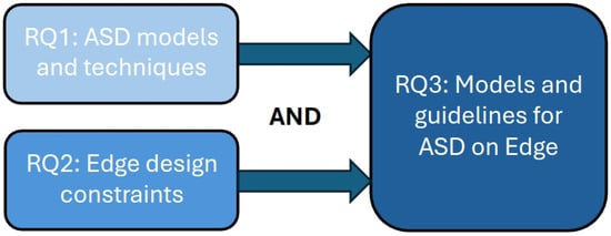
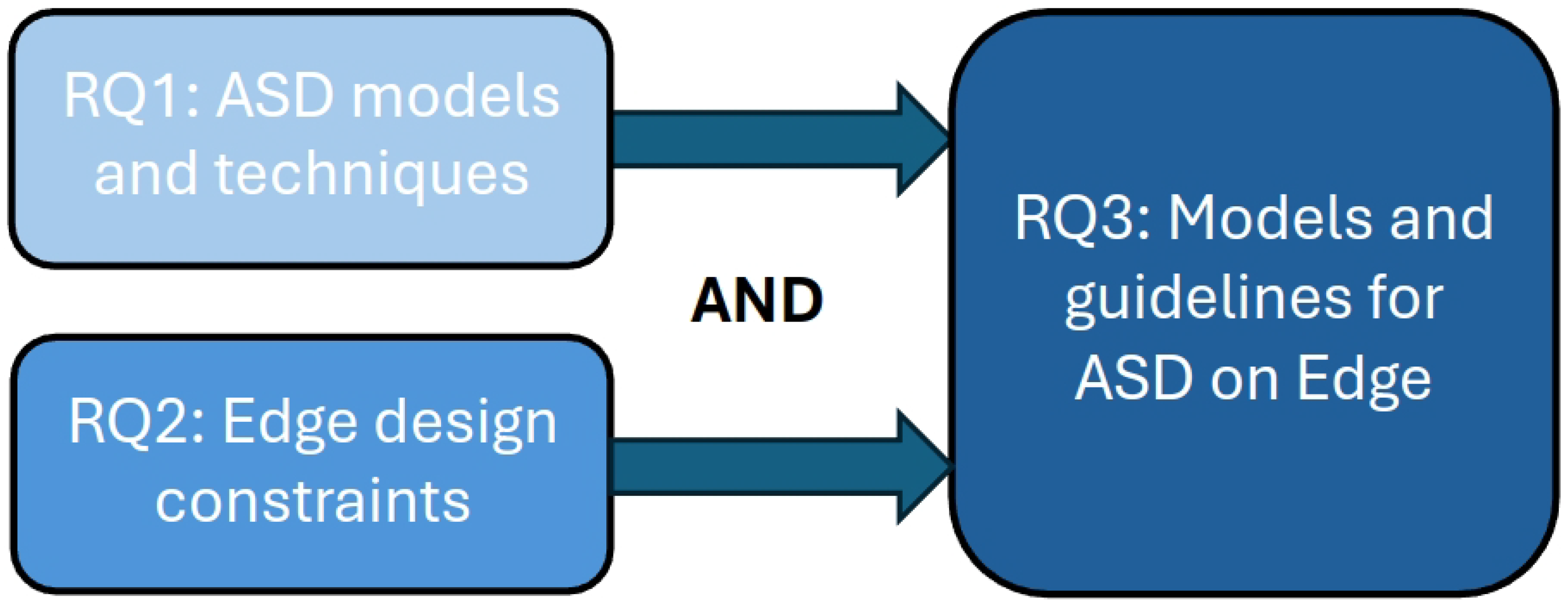
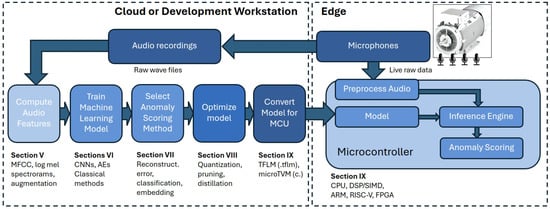
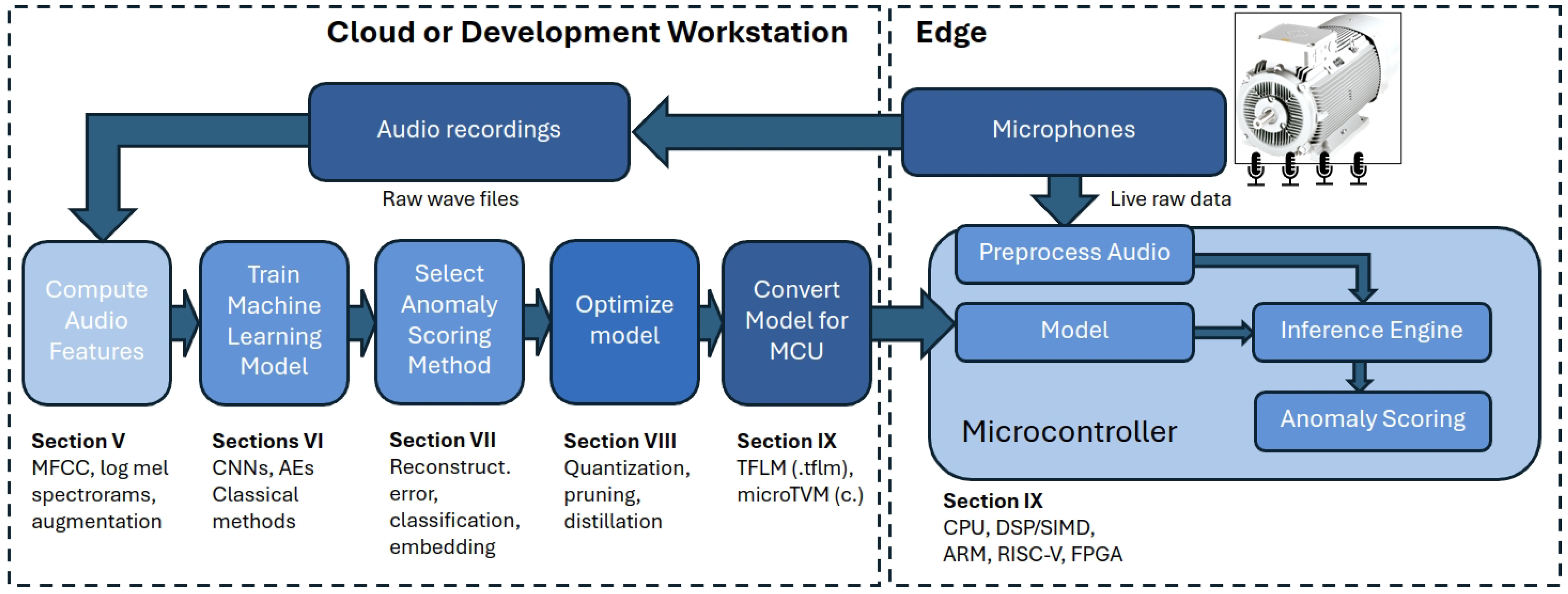
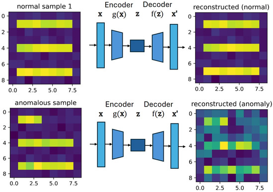
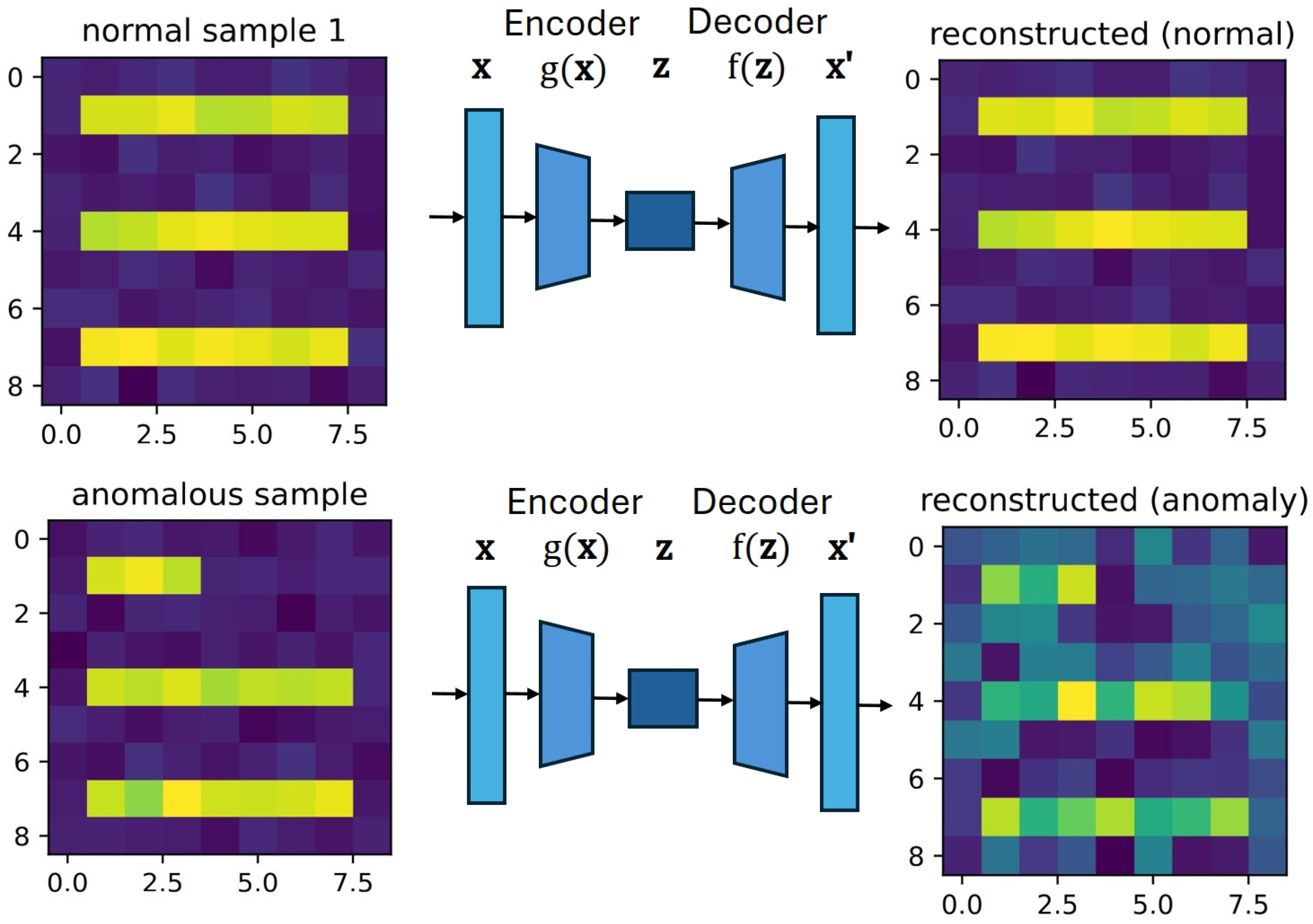
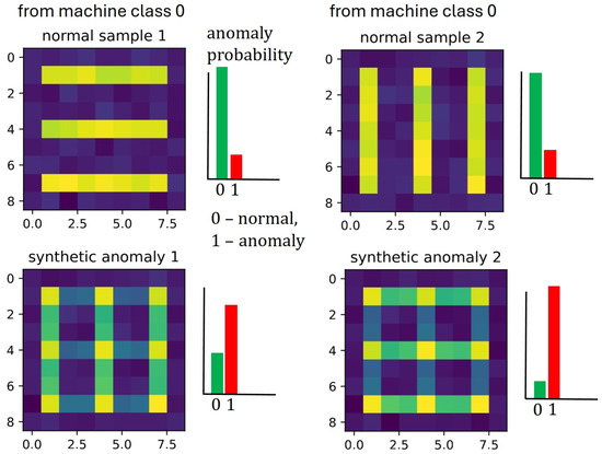
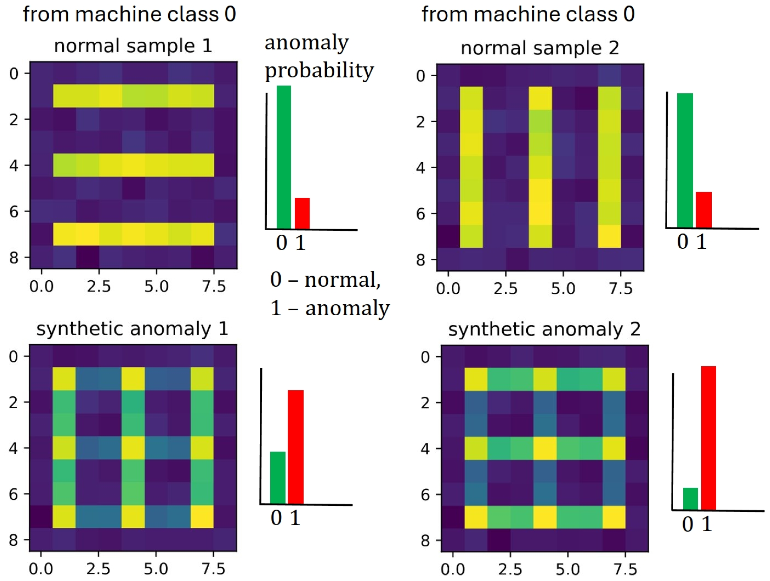
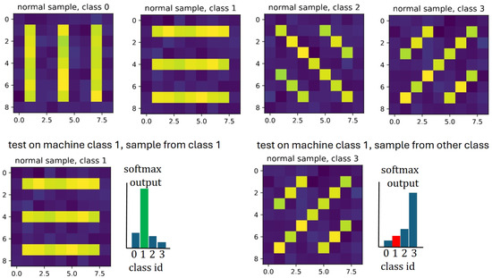
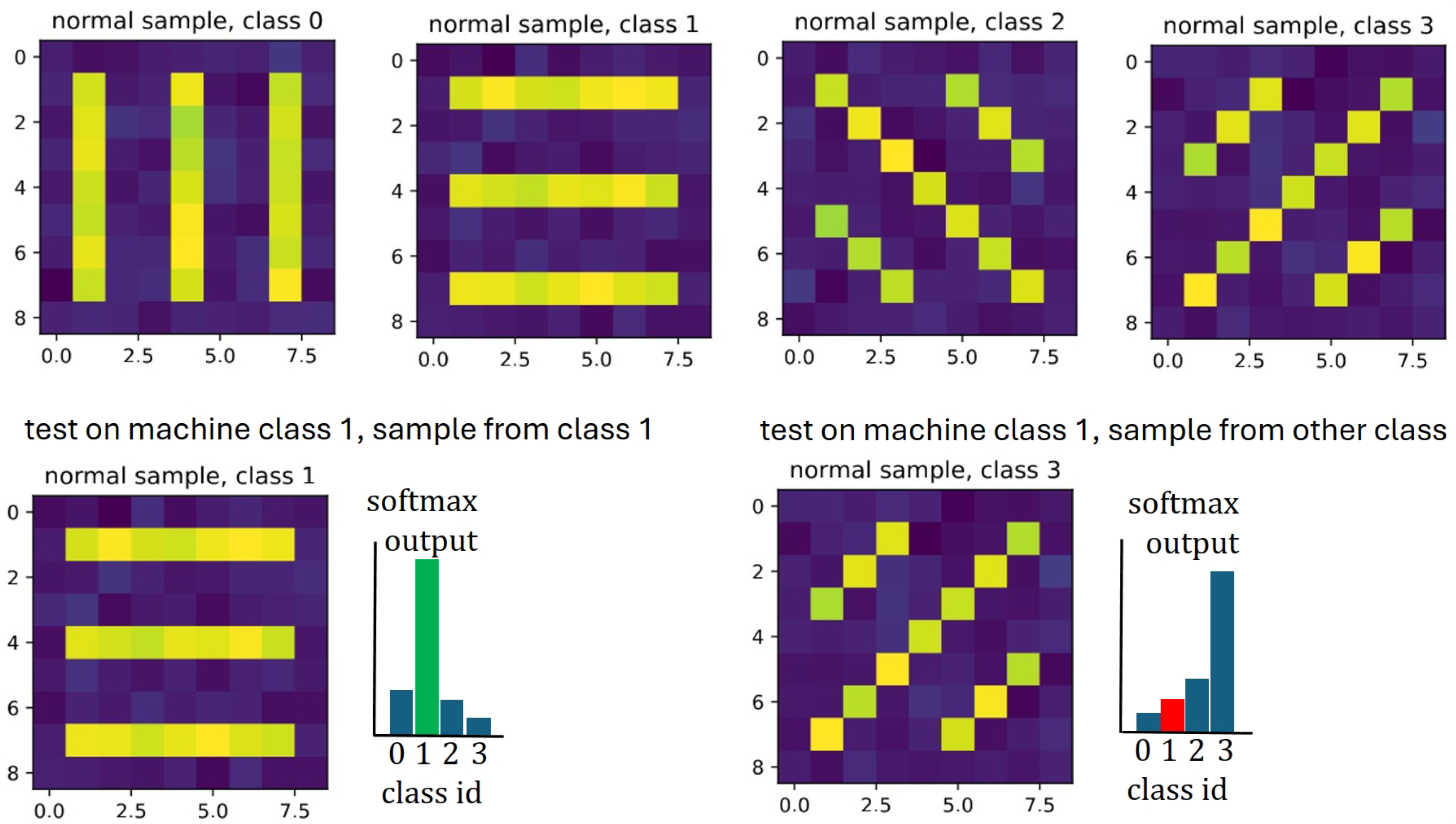
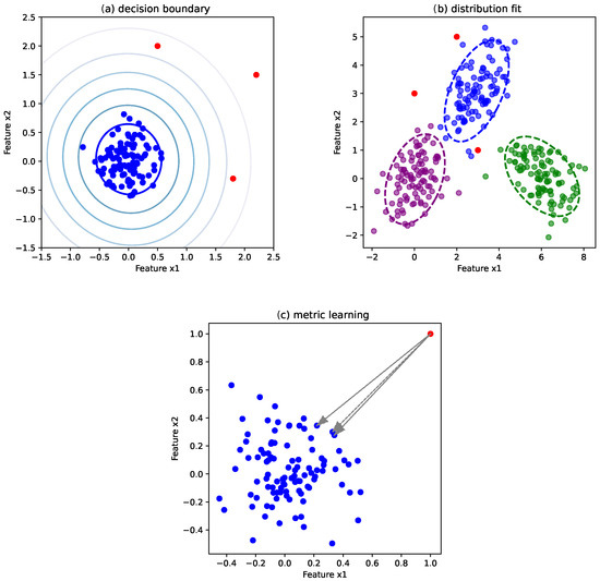
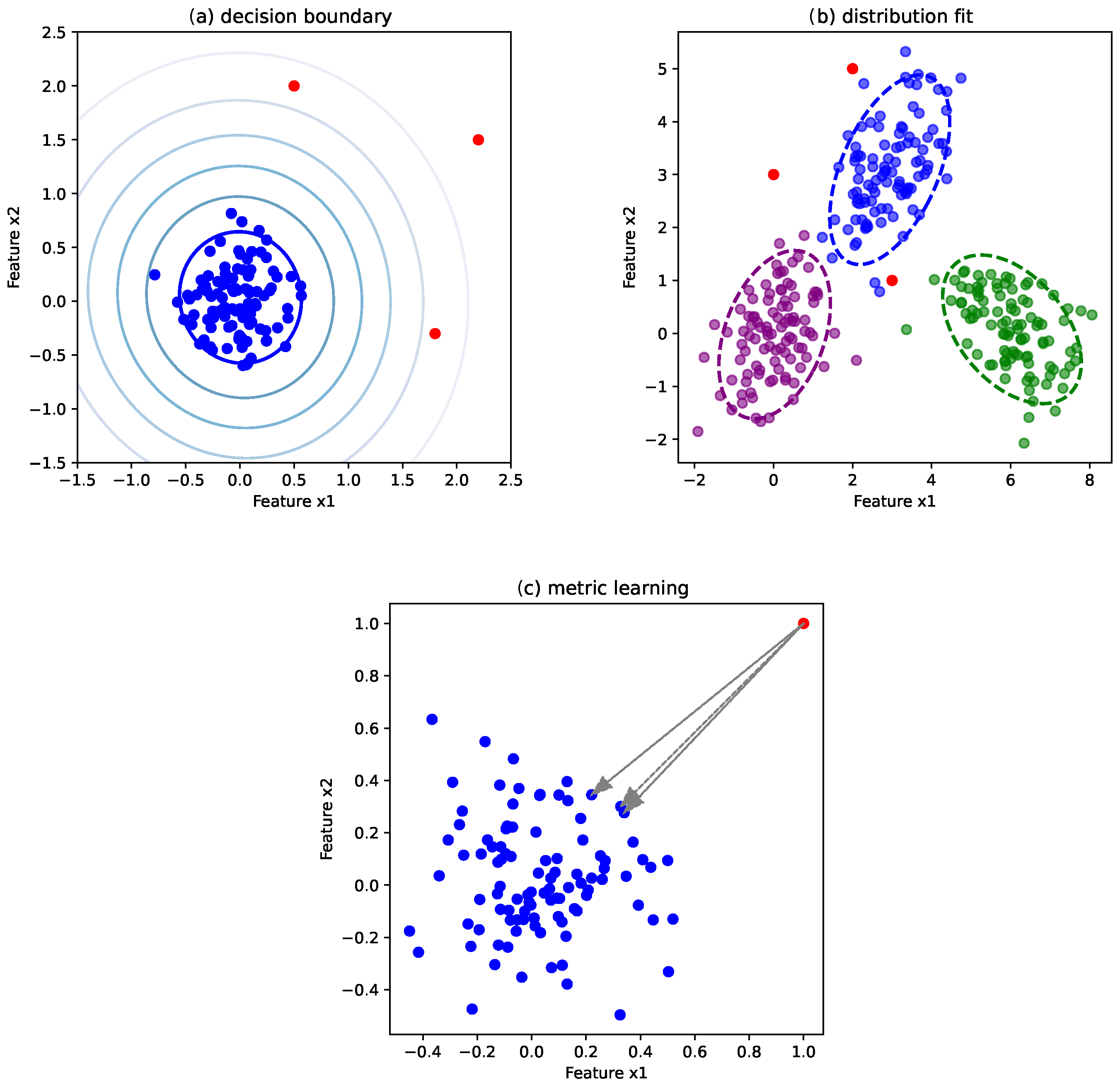
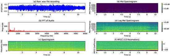
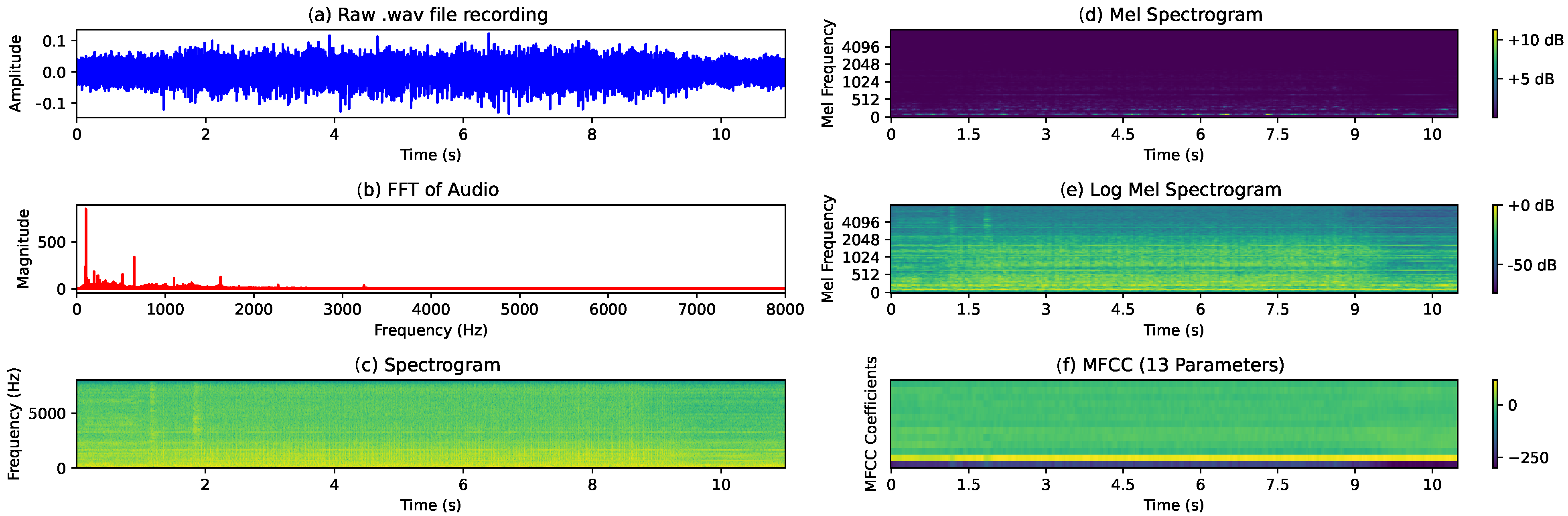
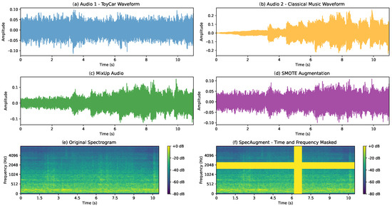
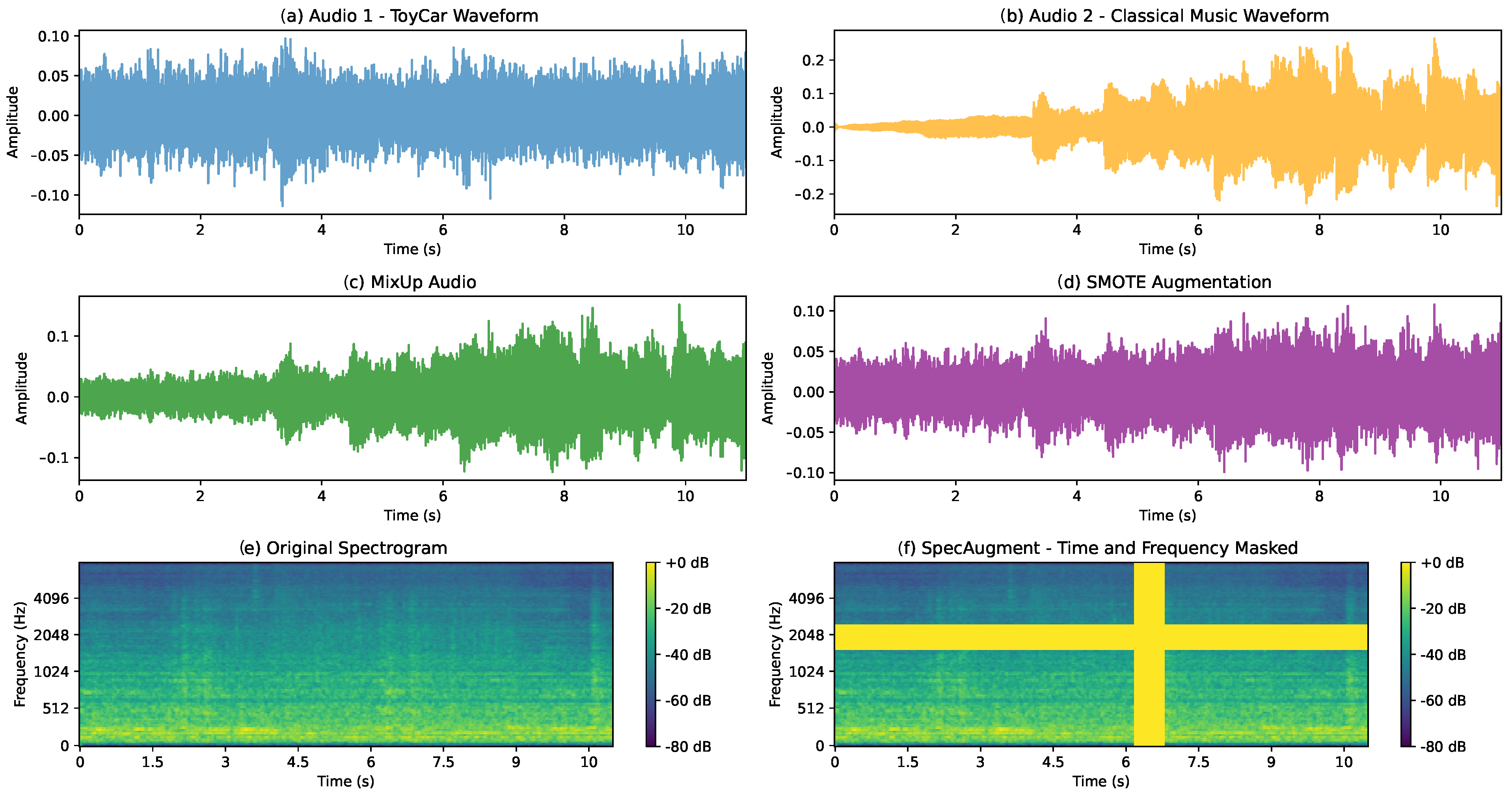

Disclaimer/Publisher’s Note: The statements, opinions and data contained in all publications are solely those of the individual author(s) and contributor(s) and not of MDPI and/or the editor(s). MDPI and/or the editor(s) disclaim responsibility for any injury to people or property resulting from any ideas, methods, instructions or products referred to in the content. |
© 2026 by the authors. Licensee MDPI, Basel, Switzerland. This article is an open access article distributed under the terms and conditions of the Creative Commons Attribution (CC BY) license.