


Abstract
The rapid growth of 5G necessitates wireless receivers capable of high-speed, low-latency communication under complex channel conditions. Traditional receivers struggle with the performance–complexity trade-off in massive MIMO systems, where linear detectors underperform and maximum likelihood (ML) detection becomes computationally prohibitive. Deep-learning-based model-driven approaches have demonstrated a favorable balance between detection performance and computational cost. However, despite their algorithmic promise, the transition of these learned detectors into practical, real-time systems is critically hampered by inefficient hardware mapping, resulting in suboptimal throughput, high resource overhead, and limited scalability. To bridge this gap, this paper presents LwAMP-Net, a dedicated FPGA accelerator for a lightweight learned AMP detector. We propose a modular and multi-mode hardware architecture for LwAMP-Net, featuring an outer-product-based dataflow that mitigates pipeline stalls and multi-mode processing elements that adapt to diverse computation patterns. These innovations jointly enhance computational parallelism and resource utilization on the FPGA. Implemented on a Xilinx XC7VX690T FPGA for a 128 × 8 MIMO system with 16QAM, the accelerator achieves a 49.2% higher normalized throughput per iteration, an 85.4% improvement in throughput per LUT slice, and a 12.7% improvement in throughput per DSP compared to the state-of-the-art methods. This work provides a complete architectural solution for deploying high-performance, hardware-efficient learned MIMO detectors in real-world systems.
1. Introduction
Fifth-generation (5G) and beyond wireless communication technologies demand significantly enhanced network capabilities, particularly in terms of supporting ultra-reliable, low-latency communications and achieving high spectral efficiency [1,2]. The pursuit of these goals, especially the latter, is largely driven by the increasing use of massive multiple-input–multiple-output (MIMO) systems, where numerous antennas are deployed at both the transmitter and receiver ends to provide higher data rates and improved spectral efficiency. However, the vast increase in antenna numbers and the complex real-world communication channels have introduced significant challenges in signal detection, making it a critical area of research.
Traditional methods for signal detection in MIMO systems, such as Maximum Likelihood Detection (MLD) [3] and linear detection algorithms, have inherent limitations. While MLD provides optimal detection performance, its complexity grows exponentially with the number of antennas, making it computationally infeasible for large-scale MIMO systems. On the other hand, linear detection methods, such as Zero-Forcing (ZF) and Minimum Mean Square Error (MMSE) [4], offer lower computational complexity but at the cost of suboptimal performance, especially under poor channel conditions. As a result, there is an urgent need for innovative solutions that can provide both low complexity and high performance to meet the demands of next-generation wireless communication systems.
In this context, deep learning (DL) has emerged as a promising paradigm for MIMO signal detection. Deep learning has been proven effective in various communication scenarios, such as signal classification and covert communication verification [5,6]. The deep-learning-based detectors can be classified as model-driven and data-driven. Initial explorations adopted data-driven methods, treating the detector as a black-box neural network trained end-to-end [7,8,9]. Such purely data-driven detectors typically require extensive training datasets and lengthy offline training periods. Moreover, their often complex and redundant network architectures lead to considerable computational overhead during inference, rendering them less suitable for real-time, low-latency systems [10]. On the contrary, model-driven approaches have gained prominence by integrating domain knowledge from classical communication theory into the DL framework [10]. These methods typically “unfold” established iterative algorithms, such as approximate message passing (AMP) [11] or orthogonal AMP (OAMP) [12], into multi-layer network structures, where parameters within each iteration layer are made trainable. For instance, OAMPNet [13] unfolds the OAMP algorithm, while LAMANet [14] offers a more lightweight learned version of AMP by simplifying the original iterative structure. More representative model-driven MIMO detectors include DetNet [15], EPNet [16], MMNet [17], LcgNet [18], DISTA [19], and so on. These model-driven detectors achieve an effective balance between performance and complexity, often outperforming their classical counterparts.
Nevertheless, most existing model-driven detectors primarily focus on algorithmic refinements, leaving a critical gap in the development of hardware-efficient architectures tailored for these learned networks. The absence of such co-designed hardware often leads to suboptimal resource utilization and implementation efficiency when these detectors are deployed, limiting their practical impact in real-world systems.
To address this gap, we propose LwAMP-Net, a model-driven MIMO detector co-designed with an efficient, FPGA-oriented hardware architecture. The proposed LwAMP-Net framework marries the iterative structure of the classical Approximate Message Passing (AMP) algorithm with trainable parameters embedded in its linear and nonlinear stages, achieving a favorable balance between detection performance and computational complexity. The core innovation of this work lies in its dedicated hardware accelerator, which features a modular and adaptively configurable architecture co-designed with the algorithm’s dataflow and parallelism characteristics. This co-design approach effectively bridges the gap between the performance gains offered by deep learning and the practical constraints of hardware deployment.
The main contributions of this paper are summarized as follows:
- We propose LwAMP-Net, a novel model-driven deep learning detector that integrates trainable parameters into the AMP framework, achieving high-performance MIMO detection with substantially reduced complexity.
- We introduce a dedicated FPGA accelerator for LwAMP-Net with a modular architecture and multi-mode processing elements. The design employs an outer-product-scheduled dataflow to eliminate data hazards and achieves high throughput with minimal resource overhead.
- We provide comprehensive experimental validation on Xilinx XC7VX690T FPGA. Our implementation achieves a 49.2% higher throughput, an 85.4% improvement in throughput per slice, and a 12.7% improvement in throughput per DSP over state-of-the-art counterparts, underscoring its superior hardware efficiency.
The remainder of this paper is organized as follows: Section 2 provides an overview of related work. Section 3 presents the LwAMP-Net model. Section 4 focuses on the hardware implementation of the LwAMP-Net detector on an FPGA platform. Section 5 gives the experimental results. Finally, Section 6 concludes the paper.
2. Related Work
2.1. Traditional MIMO Detection Algorithms
Signal detection is a critical stage in wireless receivers, tasked with the recovery and decision of transmitted symbols from received signals. Over the years, extensive research has yielded numerous detection algorithms for MIMO systems, which can be broadly categorized into optimal and sub-optimal methods based on their performance characteristics.
Optimal detection, primarily represented by Maximum Likelihood (ML) or Maximum A Posteriori (MAP) detection [3], theoretically offers the best possible performance. Its principle involves a global search over all possible transmitted symbol vectors to find the one with the minimum distance to the received signal. However, this exhaustive search is an NP-hard problem. Its complexity grows exponentially with the number of antennas and constellation points, rendering it impractical for massive MIMO systems. Variants like Sphere Decoding (SD) [20] and K-best [21] algorithms introduce controlled tree-search strategies to reduce complexity while maintaining near-optimal performance, but their exponential complexity scaling persists in large-scale scenarios.
Sub-optimal detection algorithms were developed to balance performance and complexity. The simplest among these are Linear Detection methods, including Zero-Forcing (ZF) and Minimum Mean Square Error (MMSE) detectors [4]. They recover signals through linear matrix operations but suffer from performance degradation, especially in ill-conditioned channels. While computationally simpler than ML, their requirement for matrix inversion becomes a significant burden in massive MIMO. To mitigate this, iterative matrix inversion approximations like Neumann Series Approximation (NSA) [22] and methods based on Cholesky decomposition [23] were proposed, though often at the cost of increased hardware resource consumption. Alternatively, Iterative Linear Detection algorithms, such as Gauss–Seidel (GS) [24], Successive Over-Relaxation (SOR) [25], and Weighted Jacobi (WeJi) [26], avoid explicit matrix inversion altogether by iteratively approximating the MMSE solution, thereby reducing complexity but inheriting the performance limitations of linear MMSE criteria.
To achieve performance closer to the optimal bound, Non-linear Detection algorithms are employed. These include advanced tree-search methods, Interference Cancellation (IC), and Message Passing (MP) algorithms. While they offer superior performance, their computational complexity and implementation overhead are substantially higher than linear methods. Furthermore, MP-based detectors can suffer from convergence issues in practical channels with loopy factor graphs. Therefore, the existing non-linear detection algorithms still need targeted improvements to adapt to the actual propagation conditions and to meet the requirements of hardware implementation friendliness.
Recently, physics-inspired and quantum computing-based detection have emerged as new non-linear detection paradigms for massive MIMO systems. MDI-MIMO [27] proposed a multi-stage Ising machine-based detector, which adaptively adjusts the search space to support high-order modulations up to 256-QAM and large-scale MIMO with 32 users. Meanwhile, the Quantum Approximate Optimization Algorithm (QAOA) is demonstrated to be feasible when applied to ML MIMO detection, extending the Sherrington–Kirkpatrick (SK) model with linear terms to achieve near-optimal performance with low complexity [28]. These novel approaches provide alternative solutions to the performance–complexity trade-off, but they rely on specialized physical or quantum computing platforms, which differ significantly from the practical FPGA deployment targeted in this work.
2.2. Deep-Learning-Based MIMO Detection Algorithms
The remarkable success of Deep Learning (DL) in fields such as computer vision and natural language processing has motivated its exploration for physical-layer communication tasks [29,30]. Fundamentally, MIMO signal detection involves classifying a received signal into one of a finite set of constellation points, which is a problem naturally amenable to DL-based classification approaches. DL-aided receivers demonstrate inherent potential in handling complex, non-linear, and difficult-to-model channel conditions where traditional models may falter.
Existing DL-based methodologies primarily evolve along two paradigms: data-driven and model-driven approaches. Purely data-driven methods treat the detector as a black-box deep neural network (DNN) trained end-to-end. While offering flexibility, they typically require extensive training datasets and suffer from high computational complexity during inference due to often redundant architectures, making them less suitable for real-time systems.
In contrast, model-driven approaches, which are more aligned with the focus of this work, effectively integrate established communication theory with DL. A dominant strategy is algorithm unfolding, where the iterative steps of a classical detection algorithm are unrolled into the layers of a neural network, with key parameters within each layer made trainable [31]. This paradigm has spawned several influential designs. For instance, DetNet [15] unfolds a projected gradient descent algorithm, achieving good performance under ideal channels but exhibiting complexity and robustness issues in practical scenarios. ComNet [32] demonstrates the hybrid value of combining a linear estimator (e.g., ZF) with a DNN for refinement. To better balance performance and complexity, networks based on message-passing principles have been developed. OAMPNet [13] unfolds the Orthogonal AMP algorithm, introducing trainable parameters to aid interference cancellation, though it still incurs the complexity of per-layer matrix inversion. MMNet [17], a simpler network based on the AMP framework, reduces trainable parameters significantly, enabling efficient online adaptation to different channels. More recently, LAMANet [14] introduced a machine-learning-enhanced AMP detector designed to maintain robust performance even in untrained states while co-designing an efficient FPGA architecture for real-time processing. EMMNet [33] proposed a low-complexity online learning AMP detector that prunes redundant computations in the backpropagation process and replaces complex exponential/division operations with hardware-friendly linear fitting and shift operations.
Further integrations are seen in methods like DNN-aided belief propagation [34], which embed DNNs into message-update steps to improve performance and robustness. Collectively, these model-driven detectors achieve a favorable performance–complexity trade-off, often matching or surpassing their classical counterparts. They benefit from the ability to optimize algorithmic parameters, perform joint optimization across traditional receiver blocks, and leverage mature DL design tools.
2.3. Motivation
The aforementioned studies in Section 2.1 and Section 2.2 reveal a long-standing trade-off dilemma between detection performance, computational complexity, and hardware deployability in massive MIMO uplink detection, which has not been fully resolved by existing works.
First, conventional MIMO detection algorithms suffer from inherent and insurmountable limitations in massive MIMO scenarios. The optimal maximum likelihood (ML) detection achieves the theoretical performance upper bound, but its computational complexity grows exponentially with the number of users and modulation order, making it completely infeasible for large-scale antenna configurations. Linear detection methods, including Zero-Forcing (ZF) and Minimum Mean Square Error (MMSE), have low computational complexity, but their detection performance degrades severely in ill-conditioned and spatially correlated channels, failing to meet the reliability requirements of 5G and beyond wireless systems. Classical iterative nonlinear detection algorithms, represented by Approximate Message Passing (AMP) and Orthogonal AMP (OAMP), achieve a better balance between performance and complexity. However, the AMP algorithm has a concise iterative structure but suffers from severe performance degradation and even divergence when the channel matrix deviates from the independent and identically distributed (i.i.d.) Gaussian assumption. Similarly, the OAMP algorithm improves the robustness to non-ideal channels, but introduces per-iteration matrix inversion operations, which bring prohibitive computational overhead for real-time hardware implementation.
To address these defects, model-driven deep learning detectors have emerged as a promising solution, but existing representative works still have critical bottlenecks that hinder their practical deployment. OAMPNet, which unfolds the OAMP algorithm into a trainable network, only introduces scalar learnable parameters to adjust the step size and noise estimation, resulting in limited ability to compensate for channel distortion, especially in spatially correlated channels. More importantly, OAMPNet retains the per-iteration matrix inversion operation of the original OAMP algorithm, leading to extremely high computational complexity and making it difficult to meet the low-latency and real-time requirements of practical systems. MMNet, which is based on the AMP framework, introduces a learnable linear filtering matrix and achieves near-optimal detection performance, but it must perform online training for each specific channel realization. This online training process introduces excessive latency overhead, which is incompatible with the short channel coherence time in high-mobility scenarios, and the work lacks a dedicated hardware architecture design, resulting in extremely low efficiency when mapped to actual hardware platforms. The state-of-the-art LAMANet further optimizes the model-driven AMP detector from both algorithm and hardware co-design perspectives. Specifically, it simplifies the original AMP iterative structure, removes redundant iterative calculations, designs an MMSE initialization scheme to avoid performance loss in untrained scenarios, relaxes the mandatory online training of MMNet, and implements the first real-time FPGA accelerator for learning-enhanced AMP detectors. However, while it successfully addresses the algorithmic defects of previous model-driven detectors, its hardware architecture still has inherent bottlenecks: the dedicated pipeline modules result in poor resource utilization, and its multi-stage fixed pipeline, with an oversized initiation interval, fundamentally limits the throughput upper bound, which greatly reduces its hardware efficiency in practical deployment.
To break through the above-mentioned core contradictions between detection performance, algorithmic robustness, and hardware deployment efficiency of existing model-driven MIMO detectors, this paper proposes LwAMP-Net, a lightweight learned AMP detector with a dedicated hardware–algorithm co-designed FPGA accelerator. The core design goals and advantages of this work are as follows:
- Based on the generalized AMP iterative framework, we propose a lightweight detector structure with an element-wise learnable parameter matrix. It achieves strong robustness against spatially correlated channels with offline-trained fixed parameters, eliminating the latency overhead of online training and the high complexity of per-iteration matrix inversion.
- We design an outer-product-scheduled matrix multiplication dataflow for core computing modules. This design fundamentally eliminates data dependencies between adjacent pipeline stages, reduces the pipeline initiation interval, and realizes stall-free full-pipeline operation for significantly improved detection throughput.
- We develop a multi-mode configurable processing element to enable global reuse of computing resources across modules, and adopt a unified 16-bit fixed-point format to balance detection accuracy and hardware overhead. The proposed accelerator achieves significantly higher throughput per unit resource than state-of-the-art designs.
To explicitly clarify the differences between the proposed LwAMP-Net and existing representative detectors, we summarize the core characteristics of each scheme in Table 1.
Table 1.
Characteristics comparison of different schemes.
3. Models
In this section, we propose LwAMP-Net, a model-driven signal detection algorithm. We begin by deriving a generalized framework that encapsulates various signal detection algorithms. This framework is subsequently unfolded into a neural network structure, and its key components are parameterized to form the proposed LwAMP-Net detector.
We first give the notation table, as shown in Table 2.
Table 2.
Notation table.
3.1. General Iterative Detection Framework
The Approximate Message Passing (AMP) algorithm was proposed initially for compressed sensing [11]. Consider the linear model , where represents an unknown vector in M dimensions, represents the observation vector in N dimensions, represents additive white Gaussian noise, and represents the sensing matrix (with N < M in compressed sensing). A typical iteration of the standard AMP algorithm can be expressed as:
Here, denotes the residual at iteration , is the current signal estimate, is a component-wise nonlinear denoising function, and is a scalar quantity related to . The AMP algorithm involves an iterative process between two modules. One is a linear estimation iteration based on the term in Equation (1), and the other is a nonlinear estimation iteration based on the function .
In fact, the state evolution structure of the AMP algorithm can be applied to various forms of signals, including those with amplitude or phase modulation in wireless transmission symbols. Therefore, the AMP algorithm can also theoretically be applied to the MIMO detection problem. When adapted to MIMO detection, the context differs: we generally have N ≥ M, meaning the observations are no less than the unknowns, and is a dense symbol vector rather than a sparse one. The sensing matrix corresponds to the MIMO channel matrix . After adjustment, the AMP model in the MIMO system is as shown in Equation (2):
Here, L and NL denote the linear and non-linear modules, respectively. The vector represents the output of the linear module, serving as the input to the non-linear denoiser. The scalar denotes the effective noise variance in , which is computed in each iteration.
This iterative structure corresponds to physically meaningful operations in a MIMO system. The linear module functions primarily as an interference suppressor. It processes the received signal, which is a superposition of multiple transmitted streams, to decouple them into effectively parallel, independent streams. After this linear processing, the equivalent channel for each stream can be modeled as an additive white Gaussian noise channel with a uniform signal-to-noise ratio (SNR). Consequently, the input to the non-linear module can be expressed as the true signal plus effective noise. Subsequently, the non-linear module acts as a denoiser, estimating the transmitted symbols from this noisy input. The principle of this model is illustrated in Figure 1. After one iteration, the residual interference is proportional to and typically only a fraction of the estimation error from the previous iteration. This mechanism ensures that errors diminish significantly in subsequent iterations.
Figure 1.
The physical model of the AMP algorithm in MIMO.
While AMP achieves rapid convergence and is asymptotically optimal for i.i.d. Gaussian channels, its performance degrades significantly, and it may even diverge, when the channel matrix H deviates from this strict assumption. To overcome this limitation, Orthogonal AMP (OAMP) [12] was introduced. By employing a decorrelated linear estimator and a divergence-free nonlinear estimator, OAMP relaxes the requirement on H to be unitarily invariant. The corresponding iteration is:
Here, is a normalization factor, and is proportional to the average noise power in the output of the nonlinear denoiser at the current iteration, which can be computed from the given signal-to-noise ratio and system parameters. As shown in Equation (3), compared to the standard AMP algorithm, OAMP relaxes the stringent requirement on matrix H through its decorrelated linear estimator and divergence-free nonlinear estimator. This relaxation broadens its applicability, allowing greater freedom in the choice of channel matrices, and simultaneously eliminates the need for the Onsager correction term used in AMP. However, these modifications introduce a matrix inversion operation that must be performed in each iteration, thereby increasing the computational complexity compared to the original AMP and posing a challenge for practical implementation.
Motivated by the need for a detector that is both robust to various channel conditions and computationally lightweight, we distill a general iterative detection framework from AMP and OAMP. This framework retains the essential linear cancellation and nonlinear denoising structure but simplifies the iteration by removing the intricate Onsager correction term, leading to the following generalized form:
Here, denotes the output of the linear estimation stage, while represents the result of the nonlinear estimation and also serves as the initial value for the next iteration. The calculation of is transformed as follows:
where represents the correlation matrix. Moreover, the formula of the noise reduction can be expressed as:
where and denote the standard constellation points from the chosen modulation scheme, represents the set of all possible constellation points, is the kth component of the estimate , and stands for the noise variance at the input to the denoiser.
The proposed generalized structure is designed to approximate the detection performance of AMP, relax its restrictive assumptions on the channel matrix, and maintain a computational complexity lower than that of OAMP by avoiding matrix inversion. The data flow and the interaction between the linear interference cancellation module and the nonlinear denoising module in this framework are illustrated in Figure 2. This architecture forms the basis for the subsequent network unfolding and parameterization, culminating in our proposed LwAMP-Net.
Figure 2.
The principle of MIMO iterative detection.
3.2. Network Unfolding and Parameterization
To transform the iterative framework into a trainable model, we employ the algorithm unfolding technique to propose a model-driven network. This process maps the fixed steps of an iterative algorithm onto the layered structure of a neural network. Specifically, by pre-defining a total of L iterations, the generalized detection framework in Equation (4) is unfolded into an L-layer feedforward network. Each layer corresponds to one detection iteration, sharing an identical computational structure but possessing its own set of trainable parameters. The overall architecture of this unfolded iterative detection network is depicted in Figure 3, where the data flows sequentially from the input layer (initial guess) to the output layer (final estimate).
Figure 3.
The structure of the iterative detection network.
The core innovation enabling the learning capability of this unfolded network lies in the careful parameterization of its two fundamental modules: the linear interference cancellation module and the nonlinear denoiser.
The first is the parameterization of the filtering matrix in the linear interference cancellation module. We replace the matrix in the original formulation with a trainable parameter matrix of size M × N. Simultaneously, the operation is simplified from a full matrix multiplication to an element-wise Hadamard product. The elements of are complex-valued, each corresponding to an element in the channel matrix . Consequently, can be expressed as:
in which represents the Hadamard product.
The second aspect involves the parameterization of the noise estimator in the nonlinear denoising module. The estimator can be expressed as:
where denotes the linear rectification function. The noise in is conventionally assumed to be independent and identically distributed (i.i.d.) with equal variance. In the denoising stage, would apply identically to each component of . However, when the linear module adopts the form specified in Equation (7), this i.i.d. assumption may no longer hold. Consequently, the noise variance at the input to the denoiser could differ across the various components of (i.e., across different transmit signal streams). To compensate for this variation, we introduce a trainable parameter into the noise estimator . The parameterized form of is therefore given by:
Based on the refinements described above, the general iterative detection framework from Section 3.1 has been successfully transformed into a trainable multi-layer neural network named LwAMP-Net. Each layer of LwAMP-Net contains M(N + 1) trainable parameters. The complete structure of a single LwAMP-Net layer is illustrated in Figure 4. In the diagram, the operator denotes squaring the F norm of a matrix, and represents the M-dimensional identity matrix.
Figure 4.
Schematic diagram of the single-layer structure of LwAMP-Net.
3.3. The Structure of LwAMP-Net
We have summarized a general iterative detection architecture based on the principles of AMP and OAMP in Section 3.1. Then, based on the idea of iterative expansion, the iterative algorithm was expanded into a multi-layer computing network, and a trainable multi-layer neural network, LwAMP-Net, was obtained in Section 3.2. In this Section, we will detail the calculation and iterative process of LwAMP-Net, and focus on the changes in data dimensions.
3.3.1. Linear Module
The Linear Module implements the linear computation defined in Equation (4). Its primary tasks are: (1) calculating the residual vector; (2) generating the parameterized filtering matrix ; and (3) computing the iterative update by multiplying with the residual. The residual calculation is performed in two concurrent steps using a dedicated matrix-vector multiplication module and a subtractor. Its squared norm is computed on-the-fly to avoid redundant calculations. The filtering matrix is obtained via the element-wise Hadamard product between the channel matrix H and the learnable parameter matrix , implemented using PE_B units configured in point-wise multiplication mode. The dimensional representation of the main variables involved in the above calculation process is shown in Figure 5.
Figure 5.
Linear Module Calculation Diagram.
3.3.2. Noise Estimation Module
The Noise Estimation Module is responsible for computing the noise variance vector according to Equation (9). Its primary computational tasks involve calculating the squared Frobenius norms of and , subsequently generating the final noise estimate . The dimensional transformation of the above process can be represented as shown in Figure 6.
Figure 6.
Noise Estimation Module Calculation Diagram.
3.3.3. Denoiser Module
The Denoiser Module implements the probabilistic symbol estimation defined in Equation (6). The computation begins by calculating the distance between each component of and all possible constellation points . This is implemented with 8 parallel computation units, each handling one stream. Each unit serially computes the squared Euclidean distance, normalized by the estimated noise variance obtained from the preceding module. The fixed, small number of constellation points (K = 4 for real-valued 16QAM) results in a deterministic and short latency for this step. Finally, the dimensional transformation of the above process can be represented as shown in Figure 7.
Figure 7.
Denoiser Module Calculation Diagram.
3.4. Training Configuration
In this section, we systematically describe the training configuration of the proposed LwAMP-Net, including the dataset generation scheme, end-to-end training procedure, and the selection principle of key hyperparameters.
3.4.1. Dataset Generation
All datasets used for network training and performance evaluation are generated based on the standard massive MIMO system model, with independent and identically distributed (i.i.d.) Rayleigh fading channels and spatially correlated channels are considered, respectively. All complex-valued channel matrices, transmitted signal vectors, and received signal vectors are converted into the equivalent real-valued model as described in Section 3.1 to match the input format of the neural network.
For the training dataset, we adopt a random signal-to-noise ratio (SNR) sampling strategy to ensure the generalization ability of the network in the full SNR range. The generation process is as follows:
- Channel matrix generation: For i.i.d. Rayleigh fading channels, each element of the channel matrix H follows a complex Gaussian distribution with zero mean and unit variance and is normalized by the number of transmit antennas to ensure the average received power is consistent with the transmit power.
- Transmitted signal generation: The transmitted symbol vectors are randomly generated from the standard constellation points corresponding to the modulation scheme (QPSK or 16QAM), and normalized by the average power of the modulation constellation.
- Received signal generation: The received signal is obtained after being affected by the channel and noise, and can be generated through standard MIMO simulation. The noise variance is calculated according to the randomly sampled SNR in the range of 2 dB to 15 dB for each sample, to ensure the network can adapt to different channel conditions.
- Data preprocessing: All complex-valued variables are converted into the equivalent real-valued form, and the dataset is divided into mini-batches for network training. Each batch contains 1000 independent samples with uncorrelated channel realizations.
For the test dataset, the generation logic is consistent with the training dataset, except that the channel matrix remains unchanged within one batch, and the SNR is fixed for each test scenario. Each SNR point contains 105 independent channel realizations, and 100 symbols are transmitted under each channel realization, to ensure the statistical reliability of the bit error rate (BER) and symbol error rate (SER) performance evaluation. The test dataset covers typical massive MIMO configurations, including 64 × 32 and 64 × 16, with QPSK and 16QAM modulations.
3.4.2. Training Procedure
The proposed LwAMP-Net is implemented based on the Python 3.8 TensorFlow 2.10 framework and trained in an offline supervised learning manner. We adopt a global weighted L2 loss function to ensure the layer-wise convergence of the unfolded iterative network. The loss function is defined as:
Here, B represents the batch size, L represents the number of network layers and represents the weight of each layer of the loss function. The weight increases with the layer index (the weight of the first layer is set to 0), to reduce the impact of the initial layer estimation error on the global loss and guide the network to converge to the optimal solution layer by layer.
The network training adopts the Adam optimizer, with an exponential decay dynamic learning rate strategy to balance the convergence speed and training stability. The initial learning rate is set to 0.001, with a decay coefficient of 0.96 and a decay step of 100 iterations (staircase decay mode is enabled). This strategy ensures a fast convergence speed in the early training stage, and fine-tunes the network parameters with a smaller learning rate in the later stage to avoid oscillation of the loss function. The network is trained with a mini-batch size of 1000, and the total number of training iterations is set to 5000. During the training process, the value of the loss function is monitored in real time to ensure the network is fully converged. All trainable parameters of the network are randomly initialized before training, and remain fixed after offline training is completed, without the need for online retraining for different channel realizations.
3.4.3. Hyperparameter Selection
The selection of key hyperparameters is based on the use of systematic ablation experiments to balance the detection performance, computational complexity, and hardware deployment efficiency of LwAMP-Net. The selection principle and optimal value of core hyperparameters are as follows:
- Network depth (number of unrolled iterations L): The network depth is a core hyperparameter that directly affects the detection performance. Through ablation experiments, we found that the detection performance improves with the increase in L when L < 10, while the performance saturates and even degrades slightly when L > 10 due to overfitting and error accumulation. Therefore, the optimal network depth is determined as L = 10 for algorithm performance evaluation. For FPGA hardware implementation, we adopt L = 5 to achieve a better balance between detection performance, hardware resource overhead, and detection latency.
- Training SNR range: We compared the network performance trained with different SNR sampling ranges, and determined that the random sampling range of 2 dB to 15 dB can achieve the optimal generalization performance in the full test SNR interval, avoiding performance degradation caused by insufficient training in low- or high-SNR scenarios.
- Quantization precision: During the offline training process, all parameters and calculations use 32-bit floating-point precision to ensure the convergence accuracy of the network. For FPGA hardware implementation, we adopt a unified 16-bit fixed-point format (Q1.3.12, 1 sign bit, 3 integer bits, 12 fractional bits) for all calculations, which is determined by analyzing the dynamic range of data during network inference, to balance the detection accuracy and hardware resource overhead.
4. Materials and Methods
This section presents the dedicated FPGA-based hardware architecture designed for the LwAMP-Net detector. We begin by introducing the overall system architecture, followed by detailed descriptions of its key components: the configurable processing element, the linear module, the noise estimation module, and the denoiser module.
4.1. Overall Architecture
The LwAMP-Net algorithm comprises a linear iteration stage and a nonlinear iteration stage, whose computational flow is illustrated in Figure 2. For hardware implementation, this flow is partitioned into three dedicated modules corresponding to its core operations: the Linear Module, the Noise Estimation Module, and the Denoiser Module.
These modules operate in a coordinated pipeline, as depicted in Figure 8. The Linear Module initiates computation first. Once it generates a portion of its intermediate results, they are forwarded to the Noise Estimation Module, which then begins its own processing. After both modules complete their calculations for the current data block, their outputs are fed concurrently to the Denoiser Module for the final processing stage. This sequence constitutes the computation for a single layer (iteration) of LwAMP-Net.
Figure 8.
Overall architecture.
Efficient data management is critical for sustaining this pipeline. All data involved in the detection process is stored in on-chip buffers. Dynamic data, such as the iteration vectors, channel matrix, received signal, and noise power, reside in the Input/Output Buffer. Notably, except for the iteration vectors, these inputs remain constant throughout one or multiple detection tasks, with the channel matrix being particularly invariant. Static, pre-trained network weights are stored in a separate Parameter Buffer and remain unchanged for all detections.
To prevent access conflicts and ensure uninterrupted dataflow for each module, a redundant storage strategy is employed for data shared across modules. Each module maintains its own local copy of the necessary data. Crucially, since shared data like the channel matrix is immutable during execution, this strategy does not lead to a significant increase in memory resource consumption, as only a single master copy needs to be maintained and replicated. Intermediate calculation results are not stored back to buffers but are passed directly between modules via registers. For data requiring multi-cycle computation or temporary holding, small register files are utilized for caching within the pipeline.
A brief overview of each core module’s function and resource composition is as follows. The Linear Module computes the intermediate signal estimate, the squared norm of the residual vector, and the filtering matrix, utilizing three Process Elements (PEs). Its outputs are directed to the subsequent modules: the norm and filtering matrix to the Noise Estimation Module, and the intermediate estimate to the Denoiser Module. The Noise Estimation Module, which calculates the input noise variance for the denoiser, requires several matrix multiplications and is implemented with 11 PEs and a sizable register file for intermediate caching. Finally, the Denoiser Module performs the final probabilistic symbol estimation using a softmax function (realized via a dedicated exponentiation unit) and employs 1 PE.
4.2. Configurable Process Element
An analysis of the single-layer network structure shown in Figure 4 reveals that the core computations are diverse linear algebra operations on matrices and vectors. These include matrix-matrix multiplication, element-wise matrix multiplication, matrix-vector multiplication, vector addition, and the calculation of Frobenius norms (i.e., the sum of squared elements). Although these operations differ in form, they share fundamental computational kernels. Furthermore, the network involves a small number of specialized operations, such as division and the softmax function. Considering the varying complexity and proportion of these operations within the LwAMP-Net, the underlying computational architecture adopts a strategy of general-purpose computing units augmented by specialized functional blocks.
Matrix multiplication can be decomposed into multiple vector inner products, i.e., multiply–accumulate (MAC) operations. Thus, matrix-matrix, matrix-vector, and vector-vector multiplications share the same essential computation. Similarly, element-wise matrix multiplication and scalar-vector multiplication involve only multiplication without accumulation and can be categorized together. Additionally, calculating the squared Frobenius norm (sum of squares) can also be implemented via MAC operations, where both multiplier inputs are the same matrix element. This analysis leads to two fundamental classes of computation: multiply–accumulate (MAC) and multiplication-only.
Based on this distillation, two types of general-purpose processing elements are designed for the proposed detector, as described in the following sections.
4.2.1. PE Type A
PE Type A (PE_A) is a fixed-architecture processing element optimized for vector inner-product (multiply–accumulate, MAC) operations. As illustrated in Figure 9, PE_A consists of eight 16-bit signed multipliers and seven adders arranged in a three-stage adder tree. The multipliers operate on a Q1.3.12 fixed-point format, producing 32-bit results. These results are summed by the adder tree, with bit-width extension applied at each stage to preserve precision. The final sum is re-quantized to 16 bits before being output.
Figure 9.
The structure of PE_A.
The computation is pipelined into four stages to achieve high throughput: (1) Multiplication: all eight multipliers operate in parallel; (2) First Reduction: four adders sum the eight products pairwise, yielding four partial sums; (3) Second Reduction: two adders combine the four partial sums into two; (4) Final Accumulation & Quantization: a single adder produces the final sum, which is then quantized and output.
PE_A has a parallelism factor of 8. It can compute the inner product of vectors with length ≤ 8 in a single cycle. For longer vectors, the operation is partitioned and processed over multiple cycles with accumulated results.
4.2.2. PE Type B
PE Type B (PE_B) is a configurable processing element whose computational function can be altered via configuration settings. As shown in Figure 10, its core structure, identical to PE_A, comprises eight multipliers and eight adders operating on 16-bit signed fixed-point (Q1.3.12) data. The key innovation is the introduction of configurable multiplexers at the adder inputs and output ports.
Figure 10.
The structure of PE_B.
By setting different control signals, the interconnection among the arithmetic units can be reconfigured to support three distinct operational modes. The interconnect patterns for its three modes are depicted in Figure 11. In the first mode, PE_B functions identically to PE_A as a vector inner-product unit, utilizing eight multipliers and seven adders in a four-stage pipelined tree. The second mode enables point-wise vector multiplication, where the multipliers operate independently, and their results are routed directly to the outputs. The third and most distinctive mode implements a row-wise outer-product operation: one input port broadcasts a scalar to all eight multipliers, while the other receives an eight-element vector, with results stored and accumulated via the adders. This outer-product operation leads to dimension expansion (e.g., yielding an N × M matrix from two vectors), making it computationally more intensive than an inner product. Consequently, a single PE_B computes only one row of the resultant matrix, and computing a full 8 × 8 outer product requires at least eight PE_B units operating in parallel. The outer-product capability is a primary differentiator from PE_A. Although mathematically equivalent for matrix multiplication, the inner-product and outer-product methods offer different hardware scheduling advantages; the rationale for employing the outer-product approach in specific modules is explained in subsequent sections.
Figure 11.
The connection relationships corresponding to the three modes of PE_B.
4.2.3. Matrix Multiplication Module
Both PE_A and PE_B are designed to process vectors, with a maximum parallel width of 8 elements. For vectors longer than 8, multiple computation cycles are required. Consequently, a single PE cannot complete a full matrix operation. Since practical matrix computations involve multiple vector operations, the overall latency depends on all dimensions of the matrices involved. Furthermore, as the PEs themselves are agnostic to the logical position of the data elements within the matrices, additional control logic is necessary to schedule the computation sequence and generate appropriate control signals, thereby distinguishing elements at key matrix positions. Based on this analysis, we designed a general-purpose matrix multiplication module using the proposed PEs, capable of handling matrices of arbitrary dimensions.
Matrix multiplication can be implemented in several ways, commonly through either vector inner products or vector outer products. Since PE_A and PE_B support inner and outer products, respectively, both algorithms could theoretically be realized using different PEs. A deeper analysis, however, reveals an essential difference: while mathematically equivalent, the two approaches differ fundamentally in their hardware implications. Outer-product computation leads to dimension expansion; each operation produces a matrix of the same size as the final result, which must then be accumulated element-wise with subsequent results. This necessitates storing every intermediate matrix, requiring many registers for large matrix dimensions. In contrast, the inner-product method computes only one element of the result matrix at a time, avoiding extensive intermediate storage. It is both easier to implement and more resource-efficient. Therefore, the general matrix multiplication in our design employs the inner-product method, while the outer-product approach is reserved for specific, optimized cases.
Consider multiplying matrix A (N × M) by matrix B (M × K) to produce matrix C (N × K). The inner-product method proceeds as follows: the first element C11 is obtained from the inner product of the first row of A and the first column of B; C12 from the first row of A and the second column of B; and so forth, until all elements of C are computed. The principle of this inner-product-based matrix multiplication is illustrated in Figure 12.
Figure 12.
The principle of matrix multiplication based on vector inner product.
For an N × M by M × K multiplication, a total of N × K inner products of length M are required. Given that PE_A computes an inner product for vectors of length up to 8 in one cycle, the computation is organized into three nested loops. The innermost loop, LOOP_M, iterates over the common dimension M. If M ≤ 8, LOOP_M executes once; if M > 8, LOOP_M runs for ceil(M/8) cycles, where ceil denotes rounding up. In each cycle, PE_A outputs a partial sum for a corresponding element of C; the final value for that element is obtained only after LOOP_M completes and all partial sums are accumulated. The middle loop, LOOP_K, iterates K times, cycling through each column of B to produce one complete row of C. The outermost loop, LOOP_N, iterates N times, cycling through each row of A to generate all rows of C. Following this three-loop structure, all elements of C are computed and output sequentially from the first element of the first row to the last element of the last row.
Upon completion of the entire matrix computation, a one-cycle flag signal MAT_OVER is generated concurrently with the output of the last result. This signal indicates that the current matrix operation is finished and subsequent data belong to the next matrix. It provides essential timing information for downstream modules, particularly those performing operations on an entire matrix, such as calculating the sum of squared elements. The structure of the matrix multiplication module and the principle of its three-layer loop architecture are depicted in Figure 13.
Figure 13.
Matrix multiplication structure and the principle of the three-layer loop.
4.3. The Structure of Linear Module
A key innovation in this module is the use of the outer-product method to compute the matrix-vector multiplication of and the residual, which resolves data dependency and enables a fully pipelined design. To understand the fundamental advantage of the outer-product approach, we first analyze the data dependencies inherent in both inner-product and outer-product formulations of matrix-vector multiplication.
Consider computing y = Ax, where A is an M × N matrix and x is an N × 1 vector. The inner-product method computes each element of y as:
This formulation imposes a strict sequential dependency: the computation of any output element cannot begin until all elements of the input vector x are available. Furthermore, within the computation of a single , the accumulator must complete N sequential multiply–accumulate operations before the result is valid. This creates a dependency chain that fundamentally limits the pipeline initiation interval.
In contrast, the outer-product method reformulates the computation by processing one element of x at a time:
where denotes the j-th column of matrix A. In this formulation, each term is a column vector that can be computed independently as soon as becomes available. The partial results are accumulated across iterations, but crucially, each iteration produces a complete intermediate result vector. This property fundamentally eliminates the sequential dependency constraint of the inner-product approach.
The principle of matrix multiplication based on the vector outer product is shown in Figure 14. Unlike the standard inner-product approach that requires the complete residual vector and matrix, the outer-product method allows computation to begin as soon as the first column of and the first element of the residual are available. This is realized by configuring PE_B units in outer-product mode, as shown in Figure 14, which incrementally accumulate the final result, synchronizing perfectly with the upstream data production.
Figure 14.
The principle of matrix multiplication based on vector outer product.
The overall structure and pipelined dataflow of the Linear Module are illustrated in Figure 15. For high-dimensional matrices, a vertical blocking strategy (8 rows per block) is applied to align with the PE’s parallel processing width and to minimize intermediate storage. The resulting update vector is then added to the previous layer’s estimate to produce the intermediate signal for the denoiser. This design effectively addresses rate matching and data dependency issues through outer-product scheduling, block-wise processing, and shared computation of common data, resulting in a stall-free pipeline and high hardware efficiency.
Figure 15.
The structure and calculation process of the linear module.
4.4. The Structure of Noise Estimation Module
The computation of both matrix norms is fundamentally a sum-of-squares operation, implemented by reconfiguring the matrix multiplication module. This is achieved by feeding the same matrix element to both inputs of the multipliers and reducing the computation to a double loop over the matrix rows (M) and columns (N). The squared norm of the matrix is computed sequentially in alignment with its column-wise, blocked output (8 rows per block) from the Linear Module, using a single PE_A for accumulation. This design ensures pipeline compatibility.
The calculation of presents greater complexity as it first requires the matrix product . This poses two main challenges: (1) the significant computational load compared to other operations, and (2) the column-wise output order of , which is incompatible with an inner-product based matrix multiplication and would necessitate prohibitively large register files for full-matrix caching. To address these issues, we employ an outer-product method, as shown in Figure 16. A bank of eight PE_B units operates in parallel: each PE_B computes the product between one element of a column vector from and all eight elements of a row vector from H, generating an 8 × 8 result block per cycle. The full product is accumulated through a triple-loop structure (LOOP_M, LOOP_N, LOOP_K). Furthermore, to efficiently compute , a diagonal subtraction is integrated into the accumulation process. When the loop indices indicate that the current result belongs to the output matrix’s diagonal, a value of 1 is subtracted directly from the accumulator in the corresponding PE_B, eliminating the need for a separate post-processing step. Once the M × M result matrix is obtained, its norm is computed using a single PE_A. Although the absolute latencies for the two norm calculations differ, this architecture aligns their processing rates, allowing the shorter latency to be hidden within the pipeline of the dominant computation.
Figure 16.
The vector outer product loop process in matrix multiplication.
Finally, the noise estimate vector is generated. First, the residual norm from the Linear Module is rectified via a ReLU function and multiplied by the norm of . Concurrently, the norm of is divided by two (via a 1-bit right shift) and multiplied by the input noise power . These two results are summed, and the total is divided by M (via a log2(M)-bit right shift). The resulting scalar coefficient is then multiplied by the trainable parameter vector , stored in a ROM, using a single PE_B configured for scalar-vector multiplication to produce . This vector, along with the intermediate signal estimate from the Linear Module, is forwarded to the Denoiser Module. The complete structure and dataflow of the Noise Estimation Module are depicted in Figure 17.
Figure 17.
The structure and calculation process of the noise estimation module.
4.5. The Structure of Denoiser Module
The core of the denoiser is the implementation of the softmax function to convert distances into posterior probabilities. A key observation for hardware efficiency is that the exponent argument in Equation (6) is strictly negative, confining its output to the interval (0, 1). This inherent bound eliminates overflow risks and avoids the need for complex numerical stabilization techniques like Log-Sum-Exp. To minimize hardware complexity, exponentiation is realized via a Look-Up Table (LUT), as shown in Figure 18. The LUT design leverages the bounded input range and the properties of the exponential function: for larger (more negative) inputs, the function’s sensitivity to precision diminishes. The input’s sign bit is discarded, the 3-bit integer part is preserved, and only the upper 8 bits of the 12-bit fractional part are retained for addressing, achieving a practical trade-off between area and a final output precision of 0.004. This precision is sufficient for reliable hard-decision symbol recovery. One such exponentiation LUT is shared across the 8 parallel streams. Each stream’s softmax computation sequentially calculates the exponentials of its K distances, accumulates their sum, and finally performs the division to obtain the probability vector.
Figure 18.
Precision transformation and lookup table structure.
The final step computes the denoiser’s output by taking the expectation: the probability vector for each stream is multiplied by the vector of constellation points. This is efficiently performed using the outer-product capability of a single PE_B, which computes these 8 independent weighted sums in parallel. The structure and dataflow of the Denoiser Module are illustrated in Figure 19.
Figure 19.
The structure and calculation process of the noise reduction module.
5. Results and Discussion
In this section, we present a comprehensive evaluation of the proposed LwAMP-Net detector. The performance assessment is conducted from two primary perspectives: detection accuracy and hardware efficiency. All neural network models were implemented and trained using Python with the TensorFlow framework. For hardware validation, the designed accelerator was implemented on a Xilinx XC7VX690T FPGA using the Vivado 2022.1 design suite.
5.1. Detection Performance
We begin by analyzing the impact of key architectural and training parameters on the performance of LwAMP-Net. The depth of the network, defined by the number of unrolled iterations L, is a critical factor. Figure 20 illustrates the Bit Error Rate (BER) performance of LwAMP-Net under i.i.d. Rayleigh fading channels (64 × 32 MIMO, QPSK) as a function of L. The results indicate that performance improves as L increases from a small value, benefiting from the enhanced representational capacity to mimic the iterative algorithm’s convergence. However, this improvement saturates, and a slight degradation is observed beyond an optimal point (L = 10 in our configuration). This suggests that while sufficient depth is necessary, excessive layers may introduce redundant complexity and potential overfitting, without yielding further performance gains. Therefore, L = 10 is selected as the optimal depth for subsequent evaluations.
Figure 20.
The network performance at different levels.
Next, we benchmark the detection performance of the trained LwAMP-Net against several state-of-the-art detectors under i.i.d. Rayleigh fading channels. The evaluation covers two massive MIMO configurations: 64 × 32 and 64 × 16, with both QPSK and 16-QAM modulation. The compared schemes include the optimal Maximum Likelihood (ML) detector (serving as the performance bound), the conventional MMSE linear detector, the original AMP algorithm [35], and the deep-learning-based detectors DetNet [15], OAMPNet [13], and MMNet [17]. The Symbol Error Rate (SER) performance results are summarized in Figure 21.
Figure 21.
Experimental results of the independent and identically distributed Gaussian channel. (a) 64 × 32 MIMO, QPSK modulation; (b) 64 × 16 MIMO, QPSK modulation; (c) 64 × 32 MIMO, 16QAM modulation; (d) 64 × 16 MIMO, 16QAM modulation.
The results lead to several key observations. First, all advanced detectors, including LwAMP-Net, significantly outperform the linear MMSE detector across all scenarios. Second, DetNet exhibits a noticeable performance gap compared to AMP-based learned detectors, especially for 16-QAM, highlighting the advantage of the AMP framework’s iterative interference cancellation structure. Third, while the original AMP algorithm performs well at low-to-moderate SNR, it suffers from a pronounced error floor at high SNR. In contrast, all learned detectors, including OAMPNet, MMNet, and LwAMP-Net, effectively overcome this limitation, delivering performance very close to the ML bound. The performances of LwAMP-Net and MMNet-iid are nearly identical in i.i.d. channels, which is expected given their similar mathematical foundations rooted in the simplified AMP framework.
To assess robustness in more realistic conditions, we evaluate the detectors under spatially correlated channels (Kronecker model with correlation coefficient ρ = 0.3). Figure 22 presents the SER performance for 64 × 32 and 64×16 MIMO systems with QPSK modulation, comparing LwAMP-Net with MMSE, OAMPNet, and the online-trained MMNet-correlated.
Figure 22.
The results of the spatially correlated channel experiments: (a) 64 × 32 MIMO, QPSK modulation; (b) 64 × 16 MIMO, QPSK modulation.
As expected, all detectors exhibit performance degradation under spatially correlated channels compared to the i.i.d. Rayleigh fading scenario, owing to reduced spatial diversity. Among them, OAMPNet still outperforms the linear MMSE detector but falls significantly short of MMNet. The performance of the proposed LwAMP-Net lies between that of OAMPNet and MMNet. This outcome can be attributed to the following factors. First, OAMPNet introduces only a scalar trainable parameter in its linear module, which applies a global adjustment to the filtering matrix and cannot effectively counteract the structured interference induced by channel correlations. In contrast, LwAMP-Net employs a full parameter matrix that enables element-wise adaptation, allowing it to learn and compensate for correlation patterns on a per-subchannel basis, thereby achieving superior performance in correlated environments. Second, compared to MMNet, LwAMP-Net shows a performance gap primarily because MMNet adopts online training, dynamically adapting its parameters to each specific channel realization. This approach offers an inherent advantage in handling varying channel conditions but comes at the cost of increased implementation complexity and training overhead. In contrast, LwAMP-Net operates with fixed offline-trained parameters, striking a practical balance between performance, complexity, and deployability.
The selection of benchmark algorithms and channel scenarios in this evaluation follows the standard practice in recent model-driven detection literature [14,17,36]. The chosen benchmarks cover the representative categories of linear, non-linear, and deep learning-based detectors, ensuring a comprehensive methodological comparison. Furthermore, while more complex channel models exist, the combination of i.i.d. Rayleigh and Spatially Correlated (Kronecker) channels are widely adopted in foundational works [14,17] to validate the robustness of learned detectors against channel deviations. These scenarios effectively demonstrate the algorithm’s stability and performance bounds, which serve as a solid foundation for the subsequent hardware implementation analysis.
5.2. FPGA Results
5.2.1. Performance Analysis
The proposed LwAMP-Net detector was implemented and validated on the Xilinx XC7VX690T-FFG1157 FPGA using the Vivado 2022.1 design suite. The entire design was described in Register-Transfer Level (RTL) code. Key arithmetic components, including multipliers, dividers, and block memories for the exponential lookup tables (LUTs), were instantiated using optimized Xilinx IP cores to ensure high performance and resource efficiency. Timing closure was achieved with a clock constraint of 3.5 ns, resulting in a maximum operating frequency of 286 MHz.
The hardware was configured for a 128 × 8 MIMO system (8 users, 128 receive antennas) employing 16-QAM modulation, reflecting a typical massive MIMO uplink scenario. The detector executes 5 layers (iterations) of the LwAMP-Net algorithm. All computations use 16-bit signed fixed-point arithmetic with a Q1.3.12 format (1 sign bit, 3 integer bits, 12 fractional bits). This precision was selected based on an analysis of dynamic ranges during network inference, ensuring sufficient representation accuracy while minimizing hardware overhead.
The post-implementation resource utilization of the LwAMP-Net detector on the Xilinx XC7VX690T FPGA is summarized in Table 3. The design demonstrates remarkably low resource occupancy, utilizing only 2.2% of the available LUTs, 1.2% of FFs, 3.6% of DSP slices, and 1.2% of BRAMs. This high efficiency stems directly from the lean and modular architecture presented in Section 4. The extensive reuse of configurable Processing Elements (PE_B) across the Linear and Noise Estimation modules, coupled with the streamlined data path and avoidance of bulky intermediate storage, minimizes redundant logic and maximizes the utility of each hardware component.
Table 3.
Resource consumption of the FPGA implementation.
In addition to throughput, latency and power consumption are critical metrics for real-time deployment. Based on the fully pipelined architecture described in Section 4, the end-to-end latency for processing a single detection vector is approximately 3.0 μs (equivalent to 850 clock cycles), which includes pipeline filling and draining times. This low latency satisfies the strict timing requirements of 5G slot structures. Regarding power efficiency, a detailed analysis was conducted using the power estimation tools of Vivado under typical operating conditions (50% signal toggling rate, 25 °C ambient temperature). The design yields a total on-chip power consumption of 3.25 W, comprising both static leakage and dynamic switching power. Compared to software-based implementations on general-purpose processors, this FPGA accelerator offers significantly superior energy efficiency, making it suitable for power-constrained base station units.
Scalability is a key advantage of the proposed modular architecture. The design utilizes only 2.2% of available LUTs and 3.6% of DSP slices, leaving substantial headroom for scaling to larger system configurations. The configurable Processing Elements (PEs) allow for linear resource scaling. For instance, doubling the number of receive antennas (e.g., to 256) would primarily require replicating the Linear and Noise Estimation modules, which is feasible given the current low resource utilization. Furthermore, supporting higher-order modulations (e.g., 64-QAM or 256-QAM) mainly impacts the Denoiser Module. Since the softmax operation is implemented via lookup tables, increasing constellation points would require deeper LUTs or additional BRAM resources, but the core arithmetic logic (PEs) remains unchanged. This scalability ensures that the LwAMP-Net accelerator can adapt to evolving 5G-Advanced and 6G standards requiring massive connectivity and high spectral efficiency.
In addition to scaling in antenna counts and modulation orders, the deployment of massive MIMO detectors in practical systems must consider the impact of front-end beamforming or beam-scanning techniques. Such techniques, commonly employed to enhance signal directivity and channel quality, dynamically shape the effective channel matrix observed by the baseband receiver [37]. Conventional model-driven detectors often struggle under such dynamically shaped channels. For example, linear detectors like MMSE suffer from performance degradation in ill-conditioned channels, and OAMPNet requires per-iteration matrix inversion, which becomes computationally prohibitive for large-scale arrays. More importantly, while online-trained detectors like MMNet could theoretically adapt to these variations, the required retraining latency is incompatible with the fast-varying channel coherence times typical of beam-scanning scenarios. In contrast, the proposed LwAMP-Net, with its offline-trained, element-wise learnable parameter matrix, offers a robust and practical solution. Its lightweight structure is inherently capable of adapting to a wide range of effective channel characteristics without the need for online retraining or complex per-iteration matrix inversions. This makes LwAMP-Net a highly suitable candidate for deployment in advanced wireless systems that integrate dynamic beamforming and beam-scanning techniques.
In practical application scenarios, the deployment of massive MIMO detectors is fundamentally constrained by the underlying physical propagation environment. While the algorithm–hardware co-design presented in this work is validated under standard channel models, it is essential to discuss its robustness against a wider range of practical propagation characteristics. The proposed LwAMP-Net addresses these practical challenges through two key design principles. First, the element-wise trainable parameter matrix enables per-subchannel adaptation, allowing the detector to learn and compensate for structured interference patterns. Second, by eliminating per-iteration matrix inversion and adopting a purely matrix-vector multiplication-based structure, LwAMP-Net maintains stable numerical behavior and predictable hardware timing regardless of channel conditioning, avoiding the convergence degradation or divergence issues that can plague classical AMP-based detectors in non-i.i.d. channels. This architectural stability ensures that the high hardware efficiency reported in Section 5.2.2 is sustained across diverse real-world propagation environments, making LwAMP-Net a robust and practical solution for integrated sensing and communication systems where channel conditions vary dynamically.
5.2.2. Comparison with Related Works
To comprehensively evaluate the hardware efficiency of our implementation, we compare it against five state-of-the-art MIMO detector designs, as consolidated in Table 4. The selection encompasses a spectrum of algorithmic complexities, including other learned AMP-based detectors (LAMA-Net, FD-LAMA), a traditional nonlinear detector (ISD), and advanced linear detectors (TL-BD-INSA, DN). For a fair comparison, all throughput values are normalized to an equivalent 64-QAM modulation scheme. Furthermore, for iterative detectors, the throughput is also normalized to a per-iteration basis to isolate architectural efficiency from algorithmic iteration count.
Table 4.
Comparison with related works.
The most revealing comparison is with LAMA-Net, a directly comparable learned AMP-based detector. Despite operating at a similar frequency and implementing a more demanding detection task (5 layers vs. LAMA-Net’s 3), our design achieves a 49.2% higher per-iteration normalized throughput. This gain is a direct consequence of our co-designed microarchitecture, particularly the efficient outer-product-based dataflow that minimizes pipeline stalls. More importantly, our design demonstrates superior hardware efficiency: it delivers 85.4% higher throughput per LUT and 12.7% higher throughput per DSP. The significant improvement in resource efficiency stems from two core hardware–algorithm co-design optimizations. First, the multi-mode configurable PE architecture enables global resource reuse across computational modules. The proposed reconfigurable PE_B supports three operational modes (inner-product, element-wise multiplication, and outer-product) via simple configuration signals, in contrast to the dedicated, module-specific pipeline arithmetic units in LAMANet. This unified PE design eliminates redundant multiplier–adder circuits, as the same PE array can be flexibly mapped to the diverse matrix/vector operations. Second, the outer-product-scheduled dataflow realizes a stall-free full-pipeline architecture with maximized utilization. The fixed multi-stage pipeline in LAMANet suffers from severe data dependencies between adjacent stages, resulting in an oversized pipeline initiation interval and a pipeline utilization of less than 60% in typical massive MIMO configurations.
Compared to the non-iterative ISD detector, our design exhibits lower raw throughput. However, ISD’s performance is highly sensitive to its search radius, which trades off complexity for detection accuracy. Under the compared configuration, its complexity is ≈20× that of ZF detection for only a 0.7 dB gain, whereas LwAMP-Net achieves near-optimal performance. The comparison with FD-LAMA, another AMP variant, further contextualizes our results. While FD-LAMA shows higher absolute metrics in Table 4, its performance is reported for only 3 layers and at a 50% higher clock frequency (429 MHz). When these factors are considered, the architectural efficiency of our design remains highly competitive within the same algorithm family.
Finally, the advanced linear detectors (TL-BD-INSA, DN) achieve superior raw and normalized throughput due to their fundamentally lower algorithmic complexity. However, this comes at the cost of significant performance degradation in terms of Bit Error Rate (BER) compared to near-optimal nonlinear detectors like LwAMP-Net. For instance, the BER performance of TL-BD-INSA approximates that of MMSE, and DN approaches ZF detection, both of which are substantially inferior to LwAMP-Net, especially in correlated channels. Therefore, the primary contribution of our work is not to outperform linear detectors in pure throughput, but to demonstrate that near-optimal detection performance can be achieved with a hardware-efficient, nonlinear detector architecture. Our design occupies a compelling point in the design space, offering an excellent balance between detection performance, computational complexity, and hardware efficiency that is suitable for practical high-performance systems.
6. Conclusions
This paper has presented LwAMP-Net, a novel hardware–algorithm co-design for efficient and high-performance detection in massive MIMO systems. The work addresses the critical challenge of translating the promising performance of model-driven deep learning detectors into practical, real-time hardware implementations, a gap often characterized by suboptimal throughput and high resource overhead. The core contribution is a dedicated FPGA accelerator architecture for a lightweight learned AMP detector. Key innovations include a modular and multi-mode architecture centered around an outer-product-based dataflow that reduces pipeline stalls, along with multi-mode processing elements (PE_B) that adapt to various computation patterns, maximizing parallelism and resource utilization.
Experimental validation on the Xilinx XC7VX690T FPGA for a 128 × 8 MIMO system with 16QAM modulation demonstrates the superior hardware efficiency of the proposed design. Compared to the state-of-the-art learned detector LAMA-Net, our accelerator achieves a 49.2% higher normalized throughput per iteration, an 85.4% improvement in throughput per LUT slice, and a 12.7% improvement in throughput per DSP. These results underscore the effectiveness of our co-design approach in bridging the gap between algorithmic performance and hardware deployment constraints.
In summary, this work provides a complete architectural solution that makes near-optimal, learned MIMO detection practically viable for next-generation communication systems by achieving an exceptional balance between detection performance, computational complexity, and hardware efficiency.
Author Contributions
Conceptualization, Z.L., Y.F., Y.C., L.L. and C.Y.; methodology, Z.L., Y.F., Y.C. and L.L.; software, Z.L., Y.F. and Y.C.; validation, Y.M. and J.W.; data curation, Z.L.; writing—original draft preparation, Y.F.; writing—review and editing, Z.L.; visualization, Y.F.; supervision, C.Y.; project administration, C.Y.; funding acquisition, C.Y. All authors have read and agreed to the published version of the manuscript.
Funding
This work was supported by Shaanxi Province Technical Innovation Guidance Special Project under Grant 2024ZC-YYDP-36.
Data Availability Statement
Data are contained within the article.
Conflicts of Interest
The authors declare no conflict of interest.
References
- Zhang, C.; Ueng, Y.-L.; Studer, C.; Burg, A. Artificial intelligence for 5G and beyond 5G: Implementations, algorithms, and optimizations. IEEE J. Emerg. Sel. Top. Circuits Syst. 2020, 10, 145–148. [Google Scholar] [CrossRef] [Scilit]
- Luo, F.-L. Signal Processing Techniques for 5G: An Overview. ZTE Commun. 2015, 13, 20–27. [Google Scholar]
- van Etten, W. Maximum likelihood receiver for multiple channel transmission systems. IEEE Trans. Commun. 2003, 24, 276–283. [Google Scholar] [CrossRef] [Scilit]
- Klein, A.; Kaleh, G.K.; Baier, P.W. Zero forcing and minimum mean-square-error equalization for multiuser detection in code-division multiple-access channels. IEEE Trans. Veh. Technol. 2002, 45, 276–287. [Google Scholar] [CrossRef]
- Bilal, M.; Zuberi, H.H.; Jaffar, A.; Riaz, W.; Khan, M.A.; Alharbi, A.; Miyajan, A.; Liu, S. Covert underwater communication through cepstrum modulation mimicking Pseudorca crassidens whistles using machine learning. Sci. Rep. 2026, 16, 4155. [Google Scholar] [CrossRef] [Scilit]
- Liu, S.; Zuberi, H.H.; Arfeen, Z.; Zhang, X.; Bilal, M.; Sun, Z. Spectral Efficient Neural Network-Based M-ary Chirp Spread Spectrum Receivers for Underwater Acoustic Communication. Arab. J. Sci. Eng. 2024, 49, 16593–16609. [Google Scholar] [CrossRef] [Scilit]
- Baek, M.S.; Kwak, S.; Jung, J.Y.; Kim, H.M.; Choi, D.J. Implementation Methodologies of Deep Learning-Based Signal Detection for Conventional MIMO Transmitters. IEEE Trans. Broadcast. 2019, 65, 636–642. [Google Scholar] [CrossRef] [Scilit]
- Jia, Z.; Cheng, W.; Zhang, H. A Partial Learning-Based Detection Scheme for Massive MIMO. IEEE Wirel. Commun. Lett. 2019, 8, 1137–1140. [Google Scholar] [CrossRef] [Scilit]
- Xia, J.; He, K.; Xu, W.; Zhang, S.; Fan, L.; Karagiannidis, G.K. A MIMO Detector With Deep Learning in the Presence of Correlated Interference. IEEE Trans. Veh. Technol. 2020, 69, 4492–4497. [Google Scholar] [CrossRef] [Scilit]
- Hu, Q.; Gao, F.; Zhang, H.; Li, G.Y.; Xu, Z. Understanding Deep MIMO Detection. IEEE Trans. Wirel. Commun. 2023, 22, 9626–9639. [Google Scholar] [CrossRef] [Scilit]
- Donoho, D.L.; Maleki, A.; Montanari, A. Message-passing algorithms for compressed sensing. Proc. Natl. Acad. Sci. USA 2009, 106, 18914–18919. [Google Scholar] [CrossRef] [Scilit]
- Ma, J.; Ping, L. Orthogonal AMP. IEEE Access 2017, 5, 2020–2033. [Google Scholar] [CrossRef] [Scilit]
- He, H.; Wen, C.-K.; Jin, S.; Li, G.Y. A model-driven deep learning network for MIMO detection. In Proceedings of the 2018 IEEE Global Conference on Signal and Information Processing (GlobalSIP), Anaheim, CA, USA, 26–29 November 2018; pp. 584–588. [Google Scholar]
- Brennsteiner, S.; Arslan, T.; Thompson, J.S.; McCormick, A. LAMANet: A Real-Time, Machine Learning-Enhanced Approximate Message Passing Detector for Massive MIMO. IEEE Trans. Very Large Scale Integr. (VLSI) Syst. 2023, 31, 382–395. [Google Scholar] [CrossRef] [Scilit]
- Samuel, N.; Diskin, T.; Wiesel, A. Learning to Detect. IEEE Trans. Signal Process. 2019, 67, 2554–2564. [Google Scholar] [CrossRef] [Scilit]
- Zhang, J.; He, Y.; Li, Y.W.; Wen, C.K.; Jin, S. Meta Learning-Based MIMO Detectors: Design, Simulation, and Experimental Test. IEEE Trans. Wirel. Commun. 2021, 20, 1122–1137. [Google Scholar] [CrossRef] [Scilit]
- Khani, M.; Alizadeh, M.; Hoydis, J.; Fleming, P. Adaptive Neural Signal Detection for Massive MIMO. IEEE Trans. Wirel. Commun. 2020, 19, 5635–5648. [Google Scholar] [CrossRef] [Scilit]
- Wei, Y.; Zhao, M.M.; Hong, M.; Zhao, M.J.; Lei, M. Learned Conjugate Gradient Descent Network for Massive MIMO Detection. IEEE Trans. Signal Process. 2020, 68, 6336–6349. [Google Scholar] [CrossRef] [Scilit]
- Zheng, H.; Zhang, Y.; Hu, Z.; Sun, R.; Xue, J. A Model-Driven Network Based on ISTA for Massive MIMO Signal Detection. In Proceedings of the 2022 14th International Conference on Wireless Communications and Signal Processing (WCSP), Nanjing, China, 1–3 November 2022; pp. 1–6. [Google Scholar]
- Chu, X.; McAllister, J. Software-defined sphere decoding for FPGA-based MIMO detection. IEEE Trans. Signal Process. 2012, 60, 6017–6026. [Google Scholar]
- Shen, C.-A.; Eltawil, A.M.; Salama, K.N. Evaluation framework for K-best sphere decoders. J. Circuits Syst. Comput. 2010, 19, 975–995. [Google Scholar] [CrossRef] [Scilit]
- Wu, M.; Yin, B.; Vosoughi, A.; Studer, C.; Cavallaro, J.R.; Dick, C. Approximate matrix inversion for high-throughput data detection in the large-scale MIMO uplink. In Proceedings of the 2013 IEEE International Symposium on Circuits and Systems (ISCAS), Beijing, China, 19–23 May 2013; pp. 2155–2158. [Google Scholar]
- Auras, D.; Leupers, R.; Ascheid, G.H. A novel reduced-complexity soft-input soft-output MMSE MIMO detector: Algorithm and efficient VLSI architecture. In Proceedings of the 2014 IEEE International Conference on Communications (ICC), Sydney, NSW, Australia, 10–14 June 2014; pp. 4722–4728. [Google Scholar]
- Wu, Z.; Zhang, C.; Xue, Y.; Xu, S.; You, X. Efficient architecture for soft-output massive MIMO detection with Gauss-Seidel method. In Proceedings of the 2016 IEEE International Symposium on Circuits and Systems (ISCAS), Montreal, QC, Canada, 22–25 May 2016; pp. 1886–1889. [Google Scholar]
- Zhang, P.; Liu, L.; Peng, G.; Wei, S. Large-scale MIMO detection design and FPGA implementations using SOR method. In Proceedings of the 2016 8th IEEE International Conference on Communication Software and Networks (ICCSN), Beijing, China, 4–6 June 2016; pp. 206–210. [Google Scholar]
- Peng, G.; Liu, L.; Zhou, S.; Yin, S.; Wei, S. A 1.58 Gbps/W 0.40 Gbps/mm2 ASIC Implementation of MMSE Detection for 128 × 8 64-QAM Massive MIMO in 65 nm CMOS. IEEE Trans. Circuits Syst. I Regul. Pap. 2018, 65, 1717–1730. [Google Scholar] [CrossRef] [Scilit]
- Singh, A.K.; Kapelyan, A.; Kim, M.; Venturelli, D.; McMahon, P.L.; Jamieson, K. Uplink MIMO Detection Using Ising Machines: A Multi-Stage Ising Approach. IEEE Trans. Wirel. Commun. 2024, 23, 17037–17053. [Google Scholar] [CrossRef] [Scilit]
- Gülbahar, B. Maximum-Likelihood Detection With QAOA for Massive MIMO and Sherrington-Kirkpatrick Model With Local Field at Infinite Size. IEEE Trans. Wirel. Commun. 2024, 23, 11567–11579. [Google Scholar] [CrossRef] [Scilit]
- Ruixin, G.; Yichen, L.; Yingzhuang, L.; Chen, Z. A Transformer-Based End-to-End Receiver Design for Wi-Fi 7 Physical Layer. ZTE Commun. 2025, 23, 27–36. [Google Scholar] [CrossRef]
- Bo, A.; Rongge, G.; Ruisi, H.; Mi, Y.; Yuxin, Z. A Machine Learning-Based Channel Data Enhancement Platform for Digital Twin Channels. ZTE Commun. 2025, 23, 20–30. [Google Scholar] [CrossRef]
- Xu, Z.; Sun, J. Model-driven deep-learning. Natl. Sci. Rev. 2017, 5, 22–24. [Google Scholar] [CrossRef] [Scilit]
- Gao, X.; Jin, S.; Wen, C.K.; Li, G.Y. ComNet: Combination of Deep Learning and Expert Knowledge in OFDM Receivers. IEEE Commun. Lett. 2018, 22, 2627–2630. [Google Scholar] [CrossRef] [Scilit]
- Hong, B.; Shao, H.; Wang, Z. A Low Complexity Online Learning Approximate Message Passing Detector for Massive MIMO. IEEE Trans. Very Large Scale Integr. (VLSI) Syst. 2024, 32, 1273–1284. [Google Scholar] [CrossRef] [Scilit]
- Tan, X.; Xu, W.; Sun, K.; Xu, Y.; Be’ery, Y.; You, X.; Zhang, C. Improving Massive MIMO Message Passing Detectors With Deep Neural Network. IEEE Trans. Veh. Technol. 2020, 69, 1267–1280. [Google Scholar] [CrossRef] [Scilit]
- Jeon, C.; Ghods, R.; Maleki, A.; Studer, C. Optimality of large MIMO detection via approximate message passing. In Proceedings of the 2015 IEEE International Symposium on Information Theory (ISIT), Hong Kong, China, 14–19 June 2015; pp. 1227–1231. [Google Scholar]
- Kulkarni, A.; Ouameur, M.A.; Massicotte, D. Hardware Topologies for Decentralized Large-Scale MIMO Detection Using Newton Method. IEEE Trans. Circuits Syst. I Regul. Pap. 2021, 68, 3732–3745. [Google Scholar] [CrossRef] [Scilit]
- Wang, S.; Wang, W.; Zheng, Y. Dual-Functional Quasi-Uniform Beam-Scanning Antenna Array With Endfire Radiation Capability for Integrated Sensing and Communication Applications. IEEE Trans. Veh. Technol. 2025, 74, 17829–17839. [Google Scholar] [CrossRef] [Scilit]
- Vordonis, D.; Paliouras, V. Sphere Decoder for Massive MIMO Systems. In Proceedings of the 2019 IEEE Nordic Circuits and Systems Conference (NORCAS): NORCHIP and International Symposium of System-on-Chip (SoC), Helsinki, Finland, 29–30 October 2019; pp. 1–6. [Google Scholar]
- Li, K.; Jeon, C.; Cavallaro, J.R.; Studer, C. Decentralized equalization for massive MU-MIMO on FPGA. In Proceedings of the 2017 51st Asilomar Conference on Signals, Systems, and Computers, Pacific Grove, CA, USA, 29 October–1 November 2017; pp. 1532–1536. [Google Scholar]
- Wang, H.; Ji, Y.; Shen, Y.; Song, W.; Li, M.; You, X.; Zhang, C. An Efficient Detector for Massive MIMO Based on Improved Matrix Partition. IEEE Trans. Signal Process. 2021, 69, 2971–2986. [Google Scholar] [CrossRef] [Scilit]
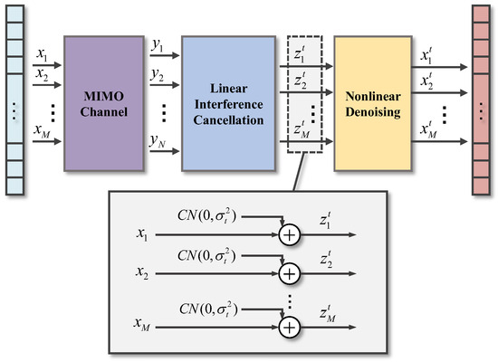
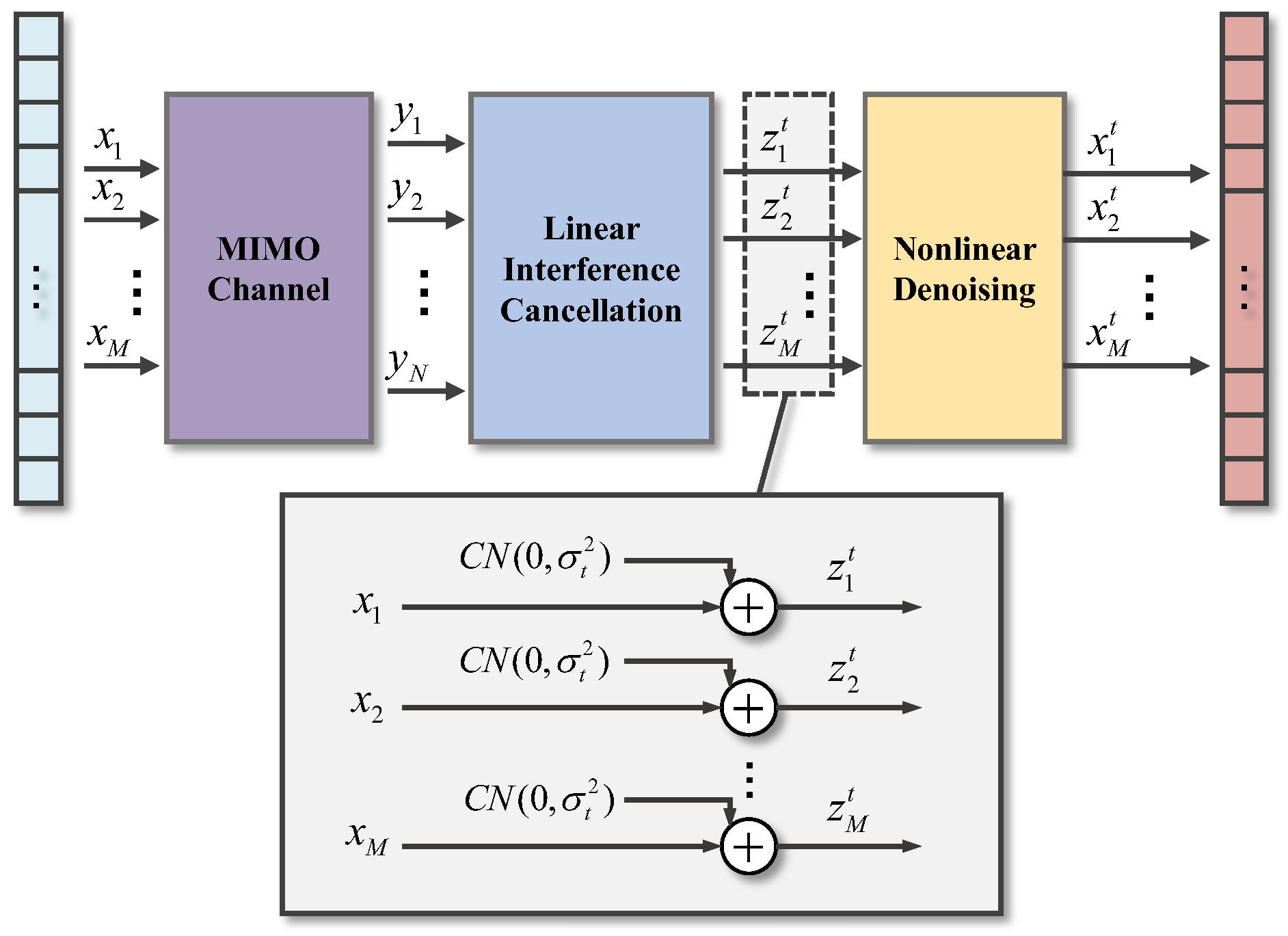
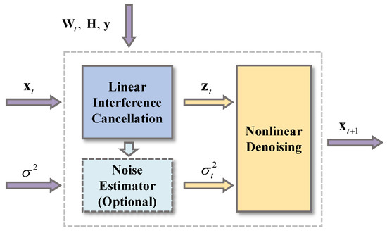
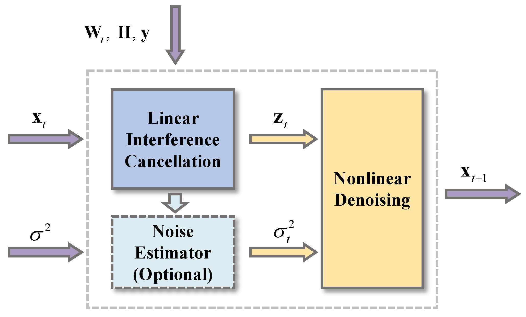
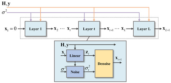
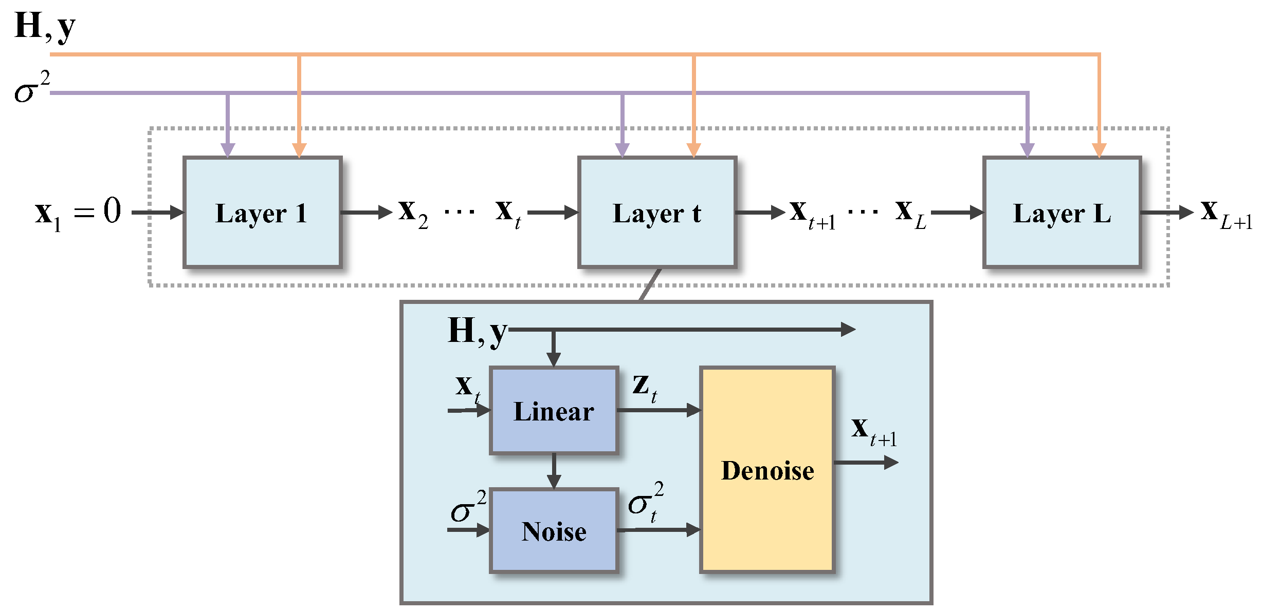
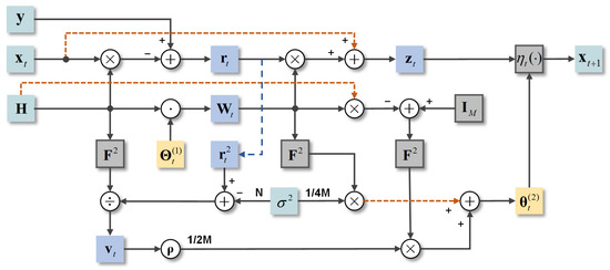
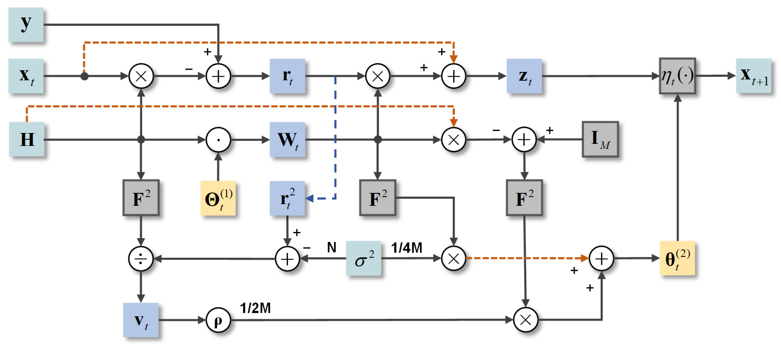
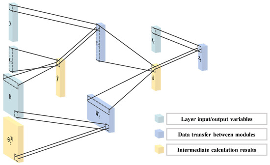
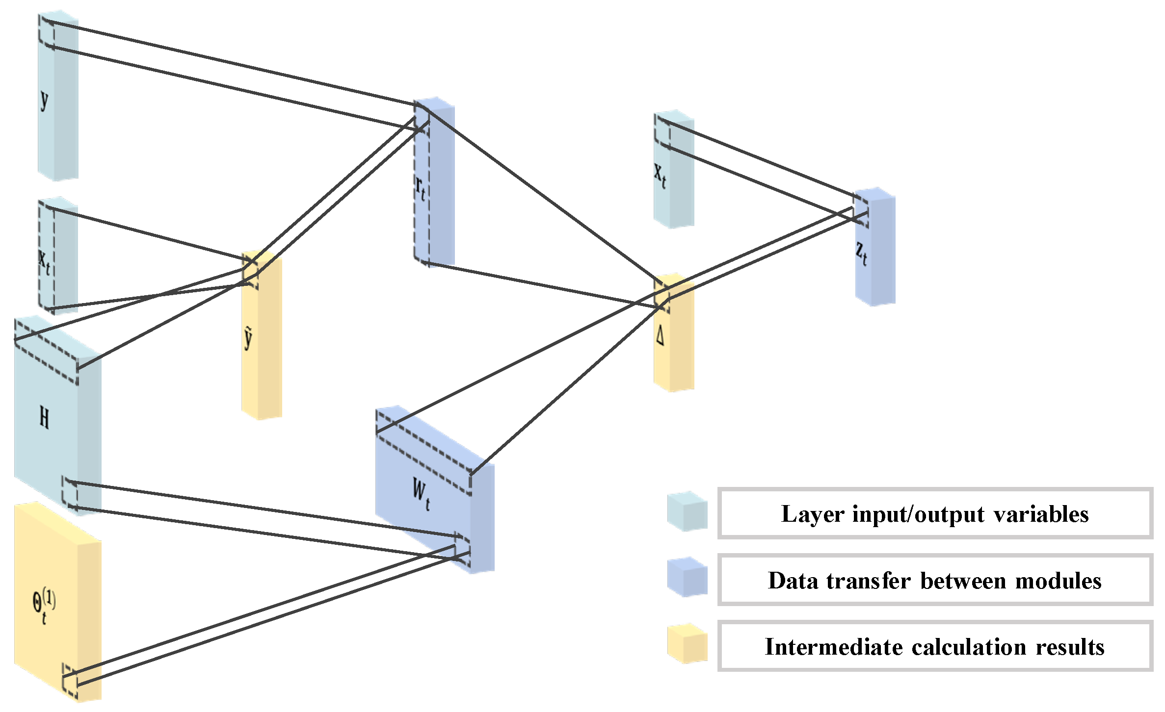
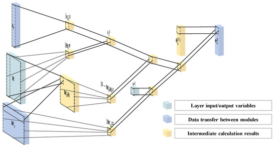
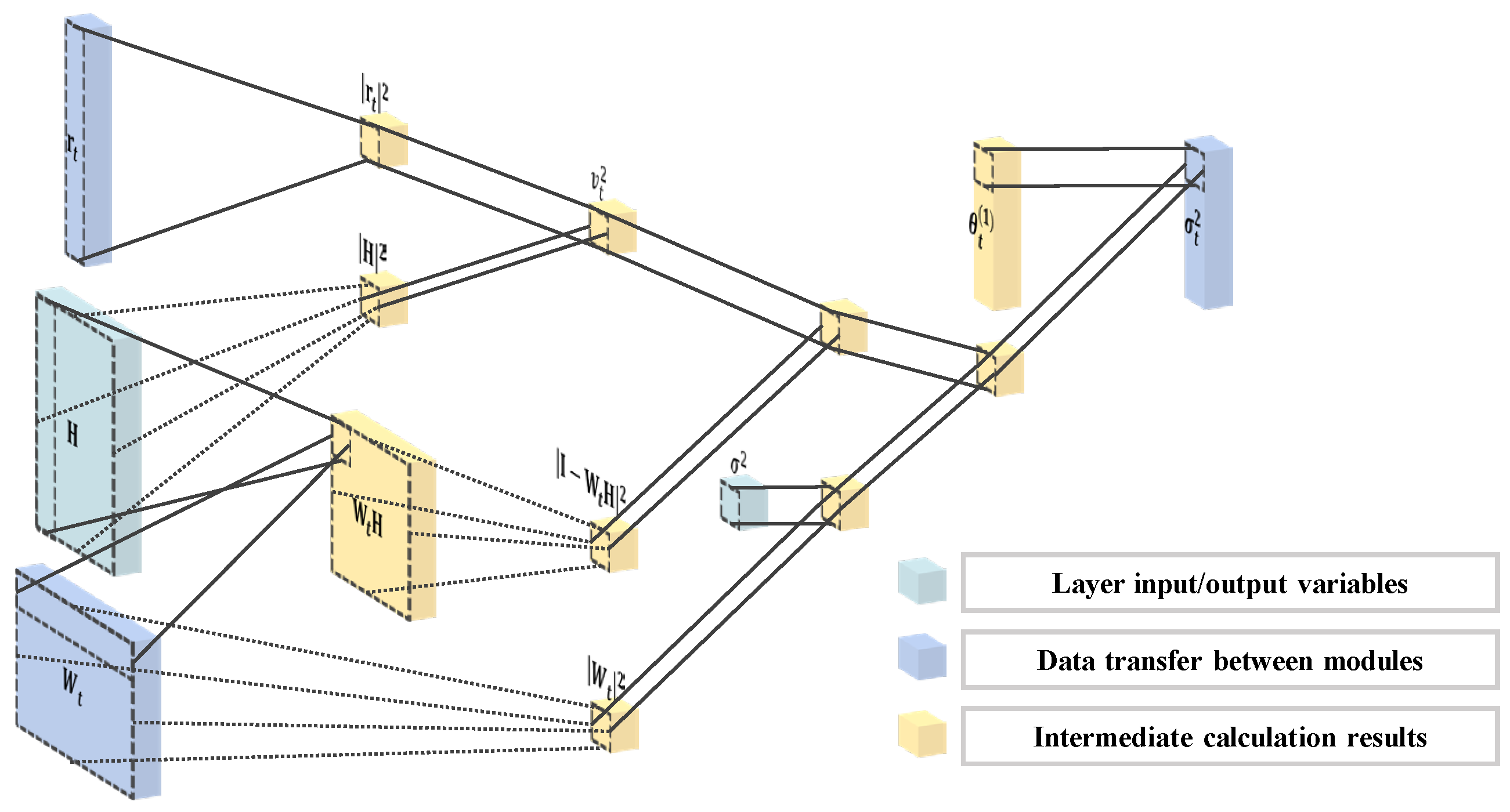
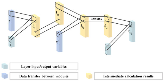
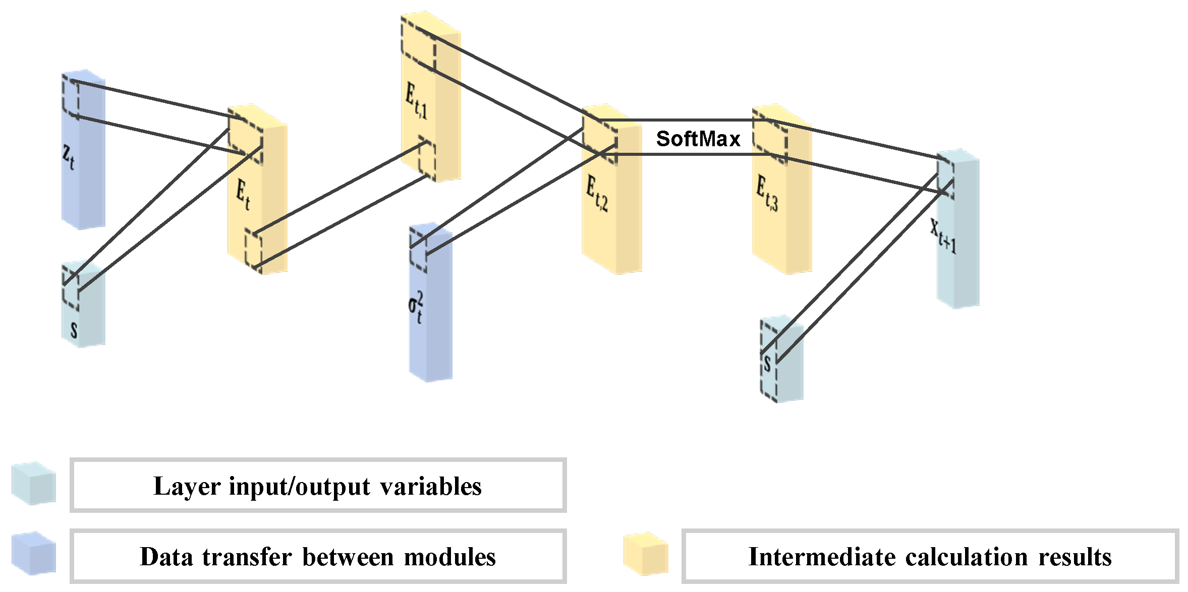
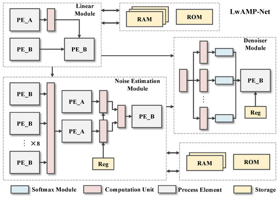
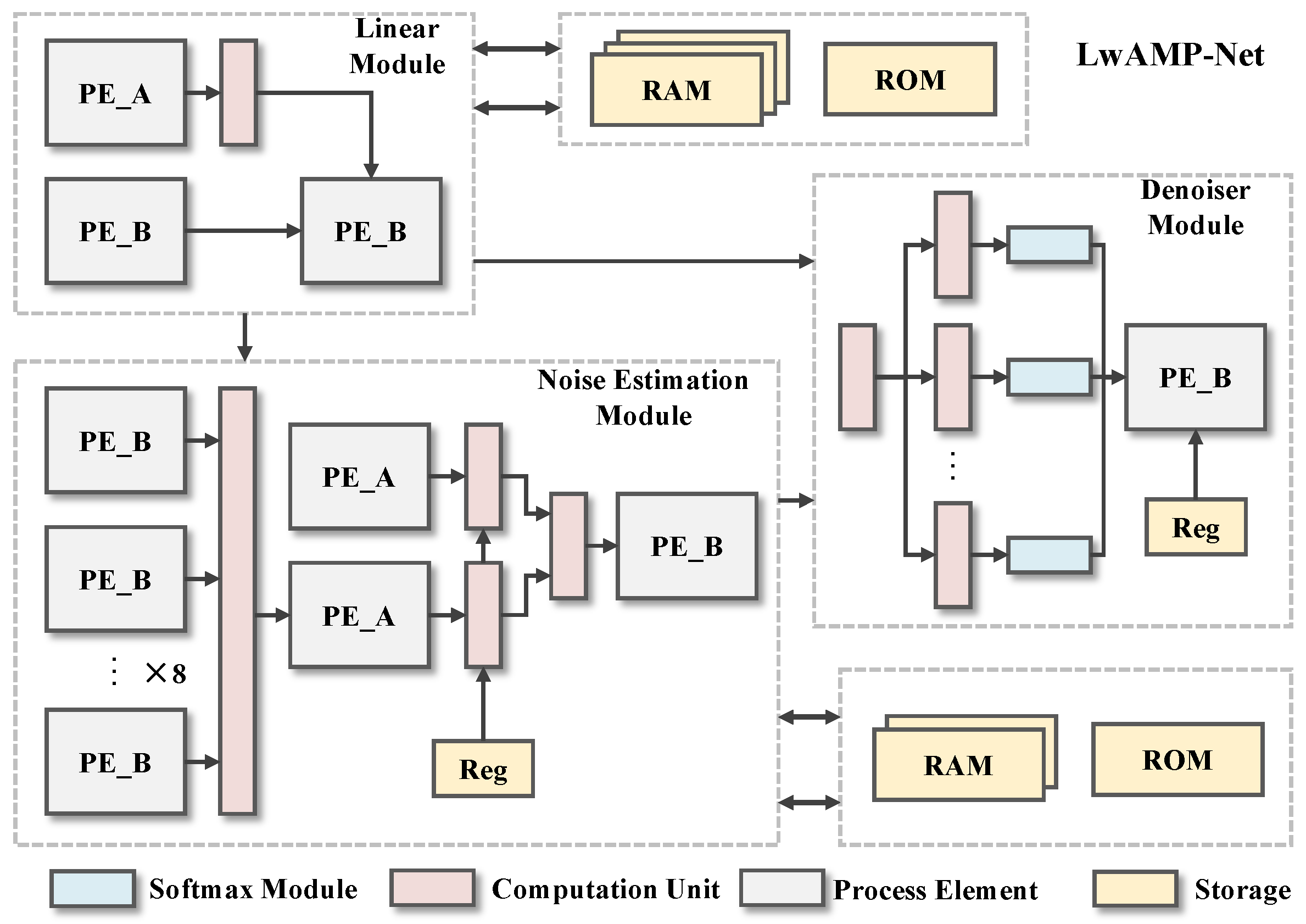
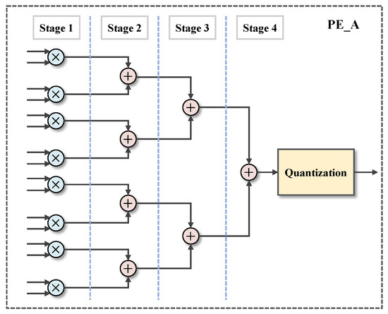
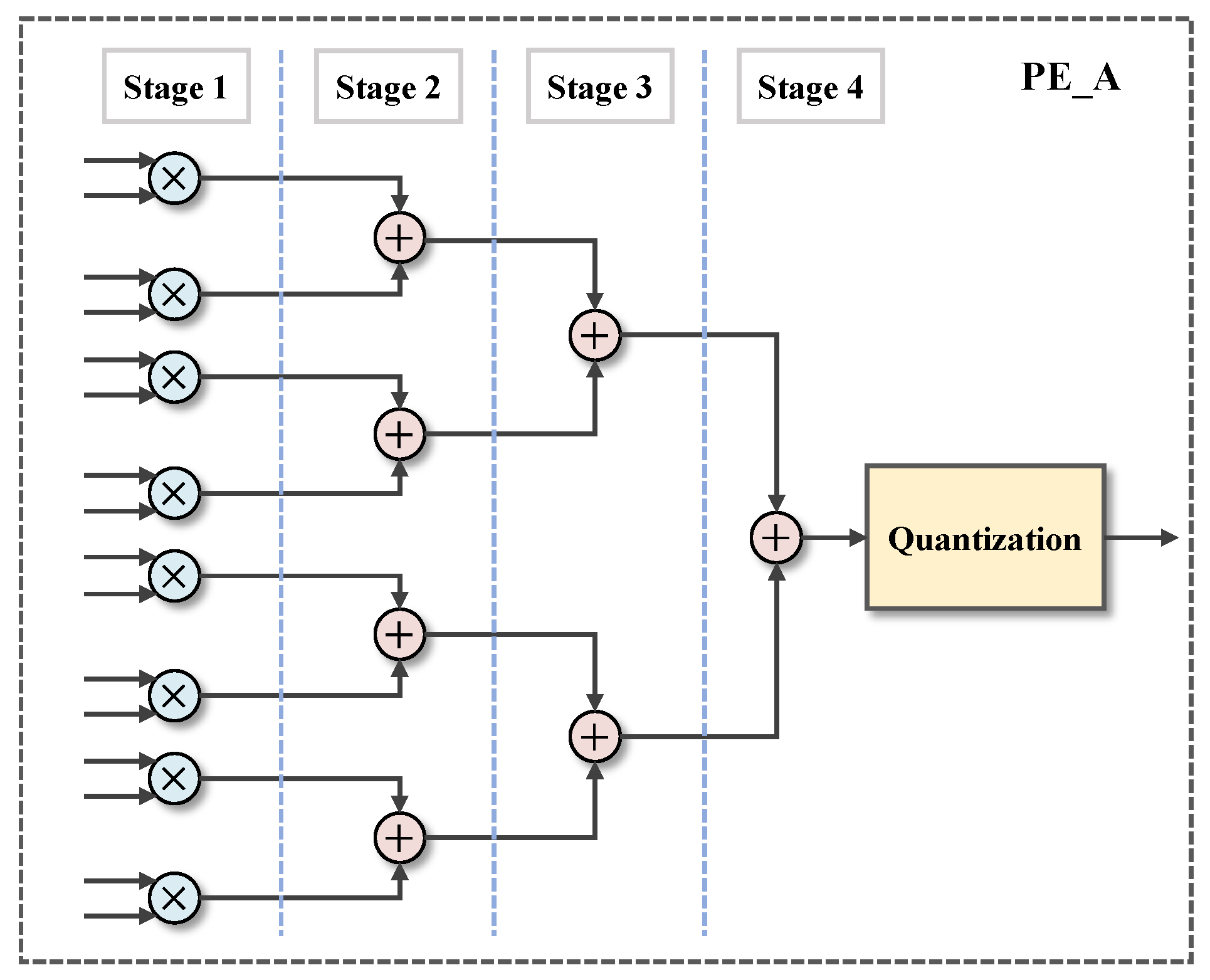
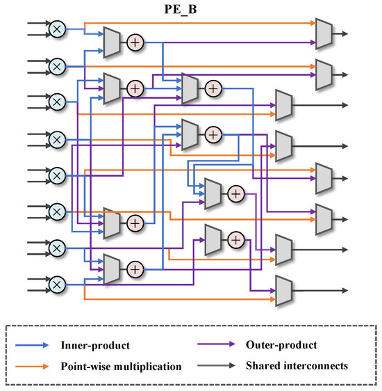
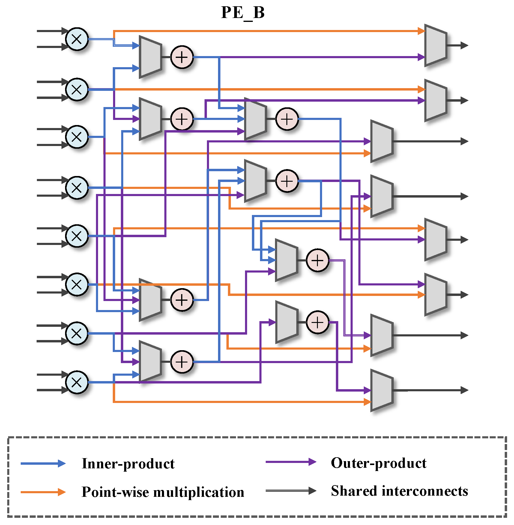
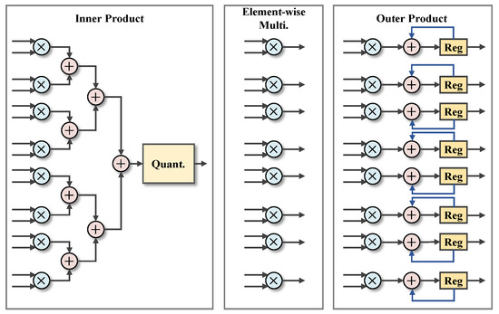
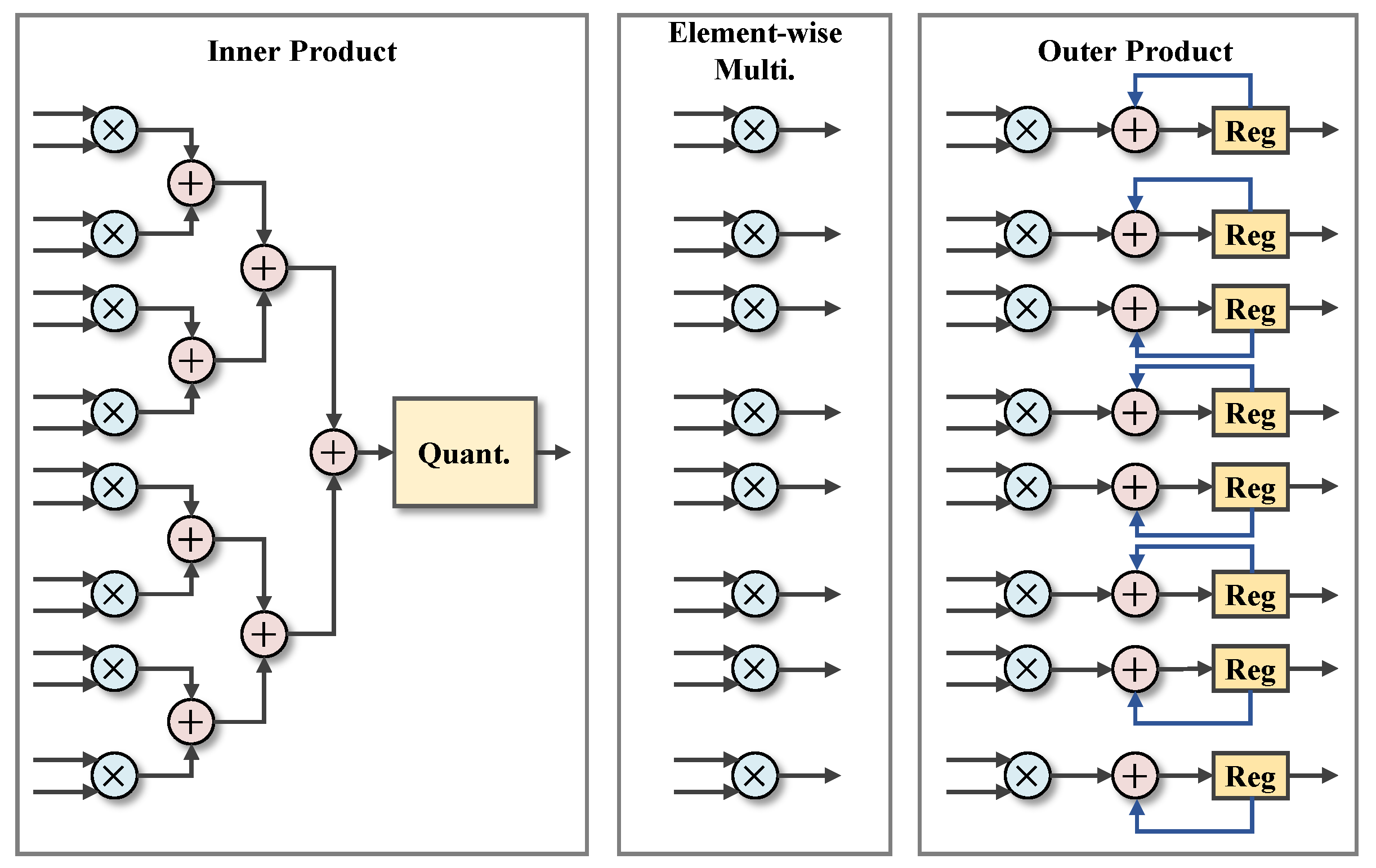
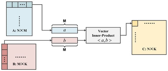
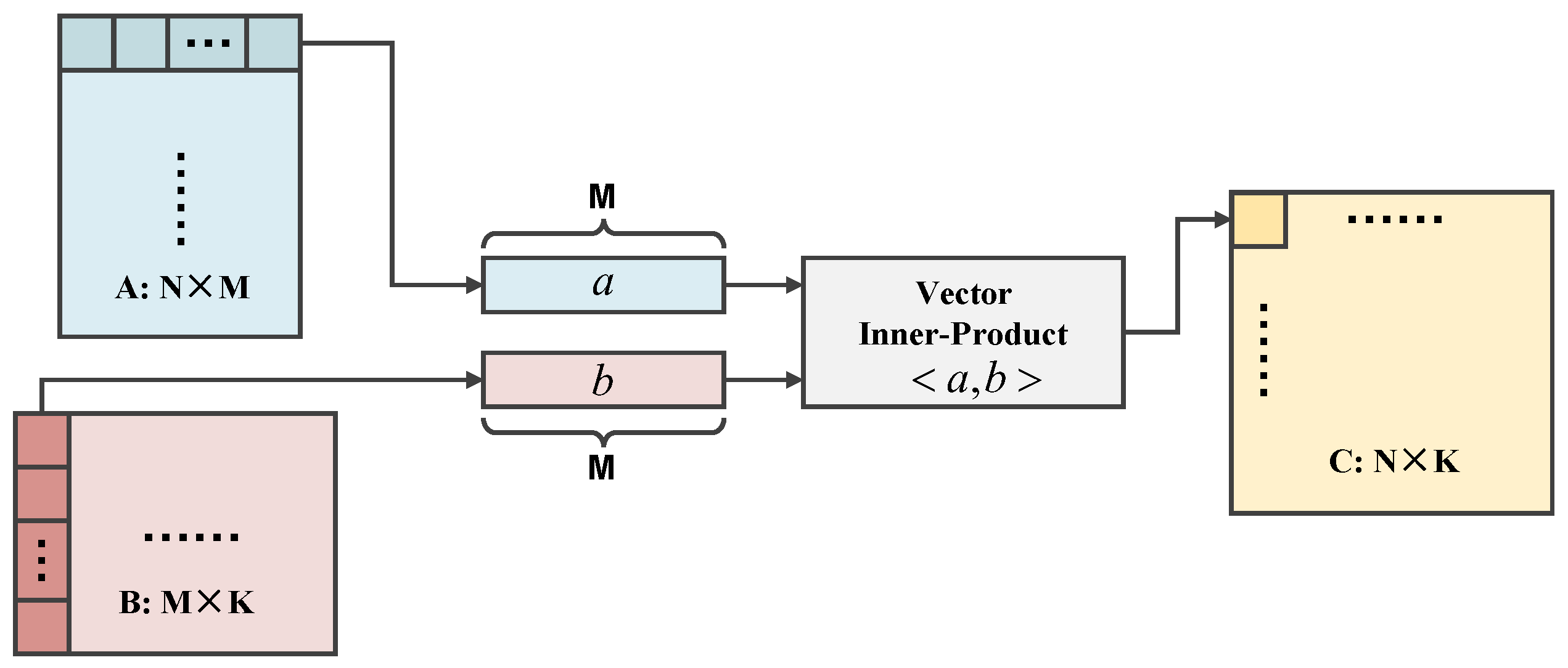
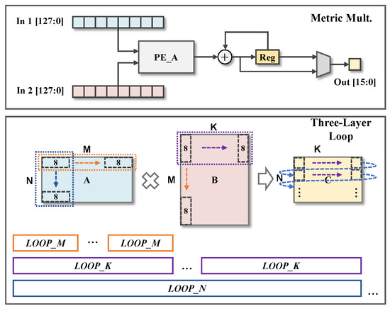
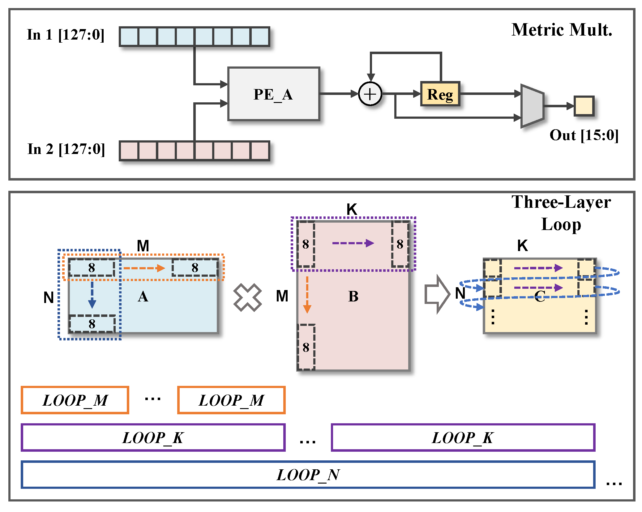
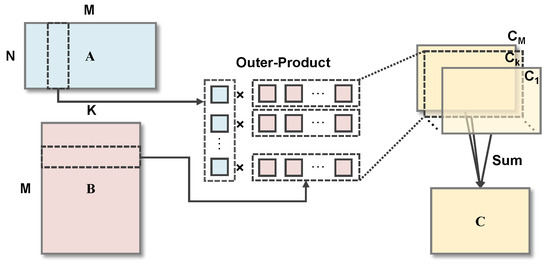
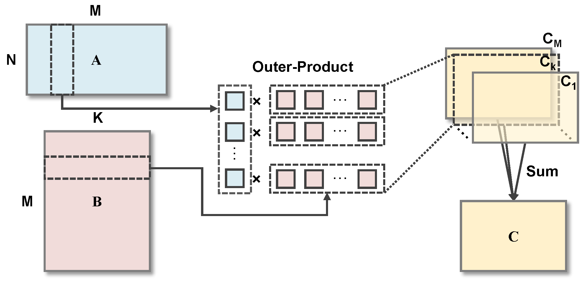
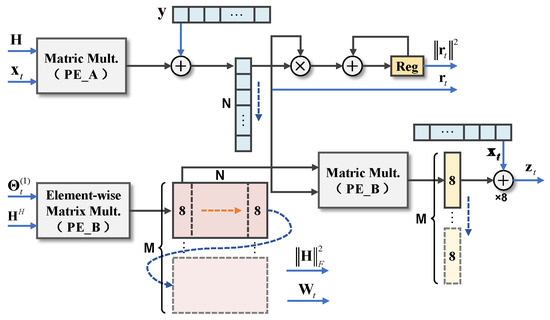
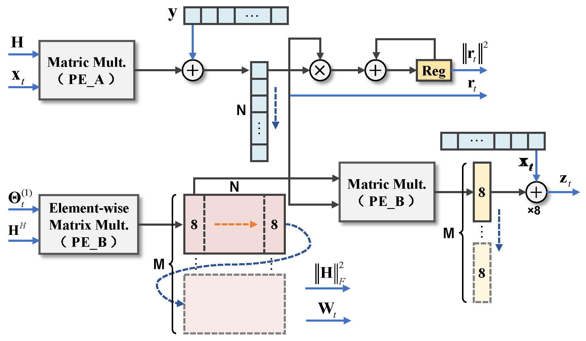
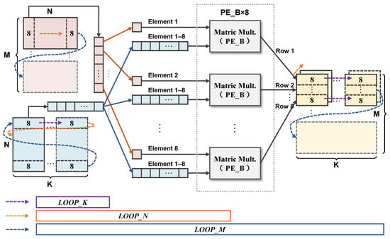
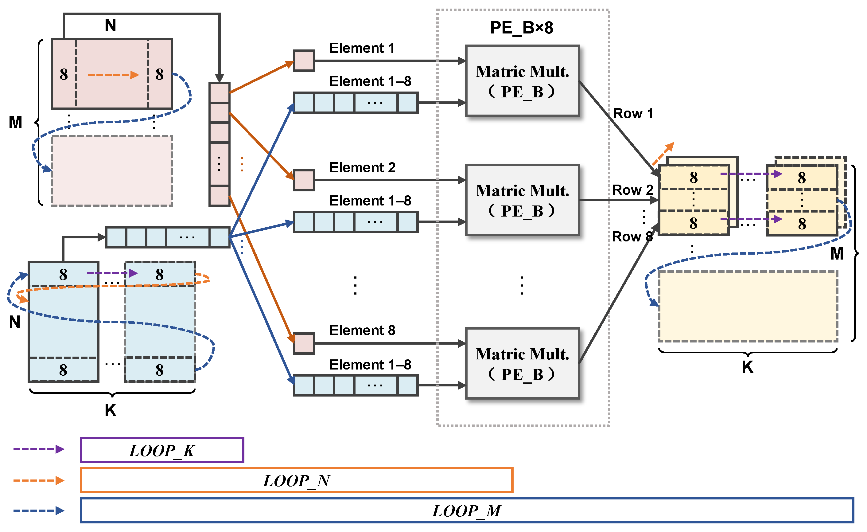
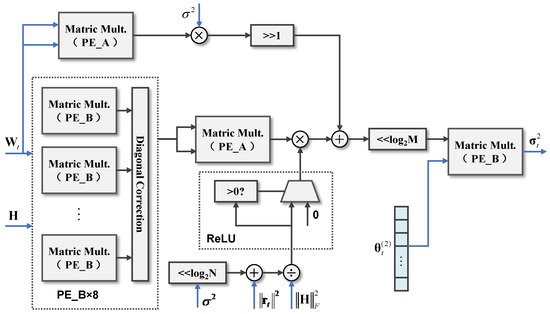
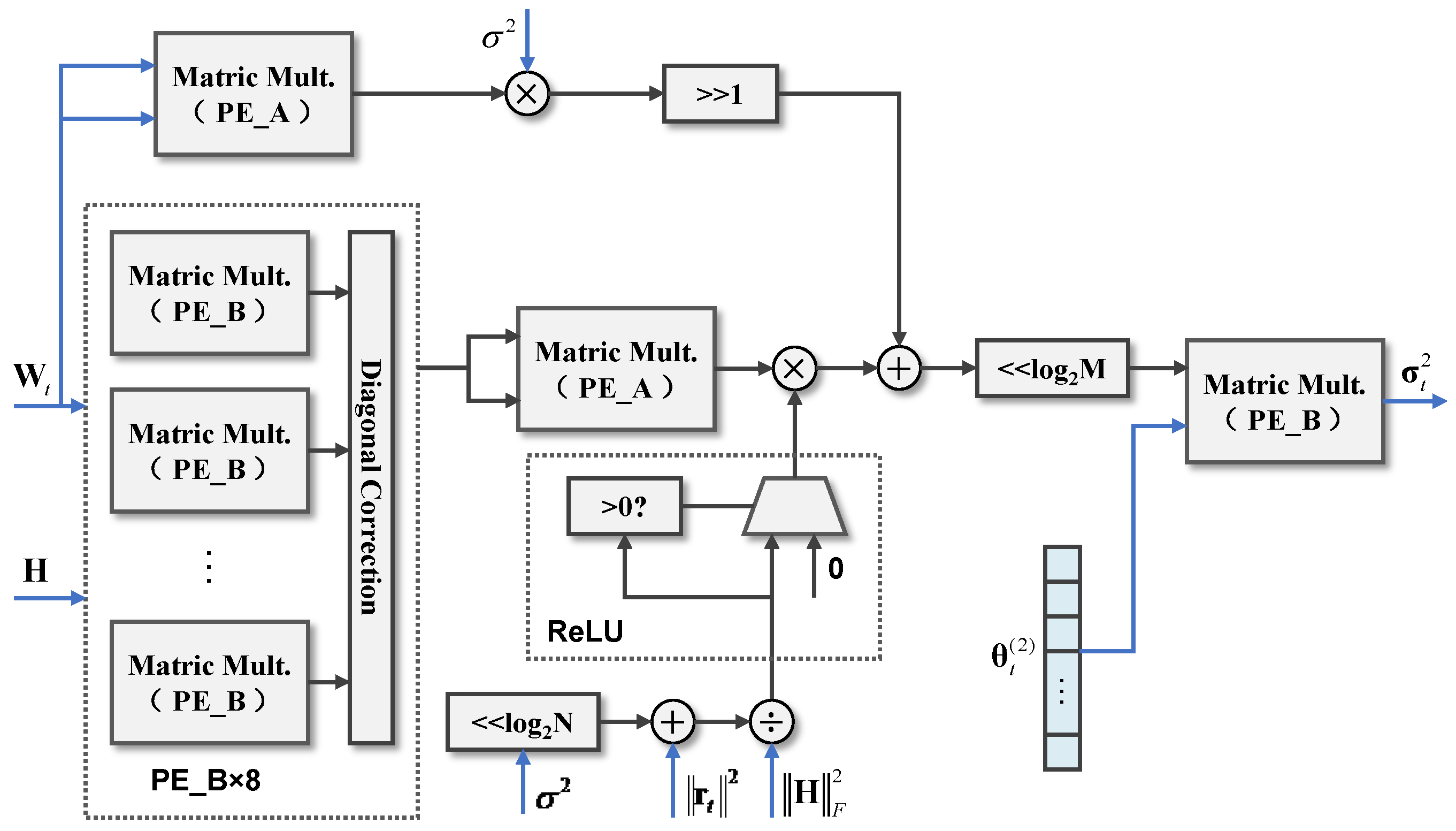
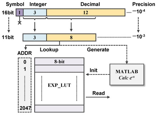
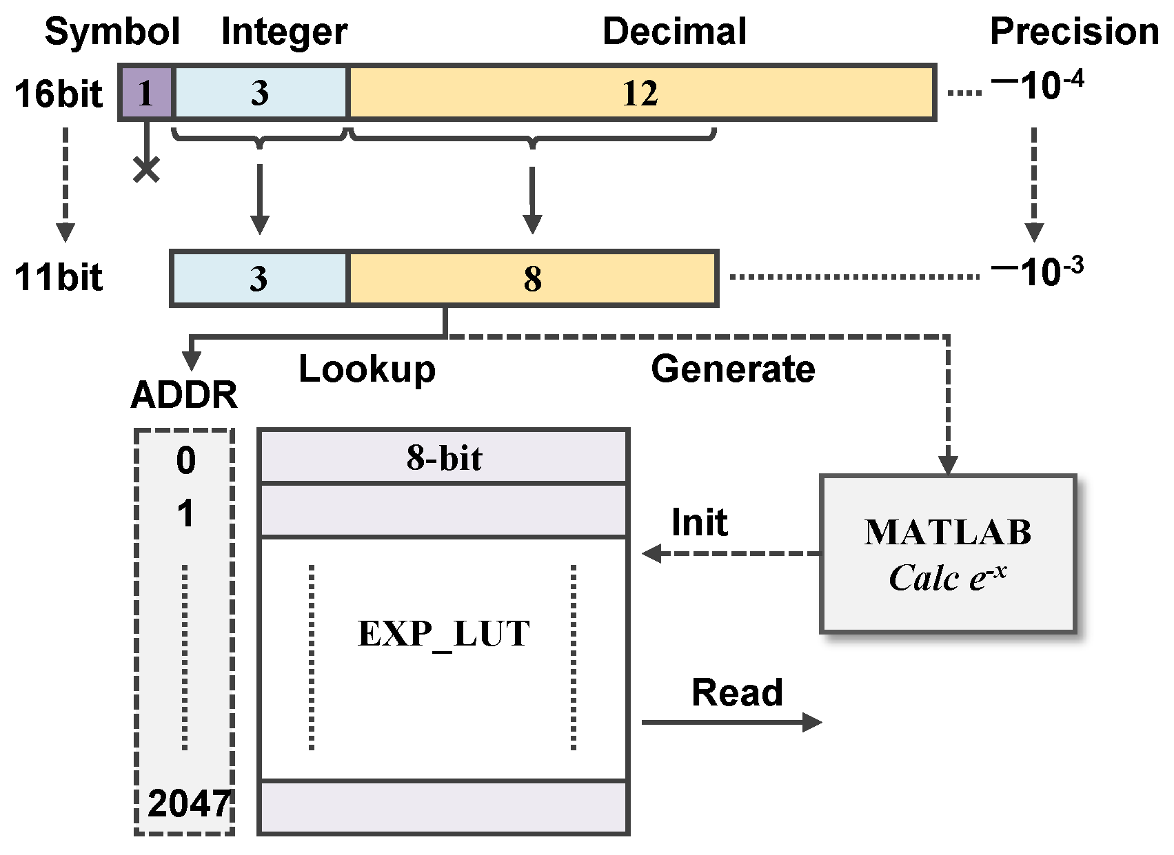
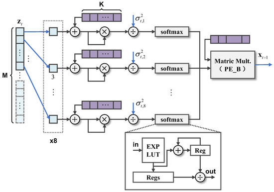
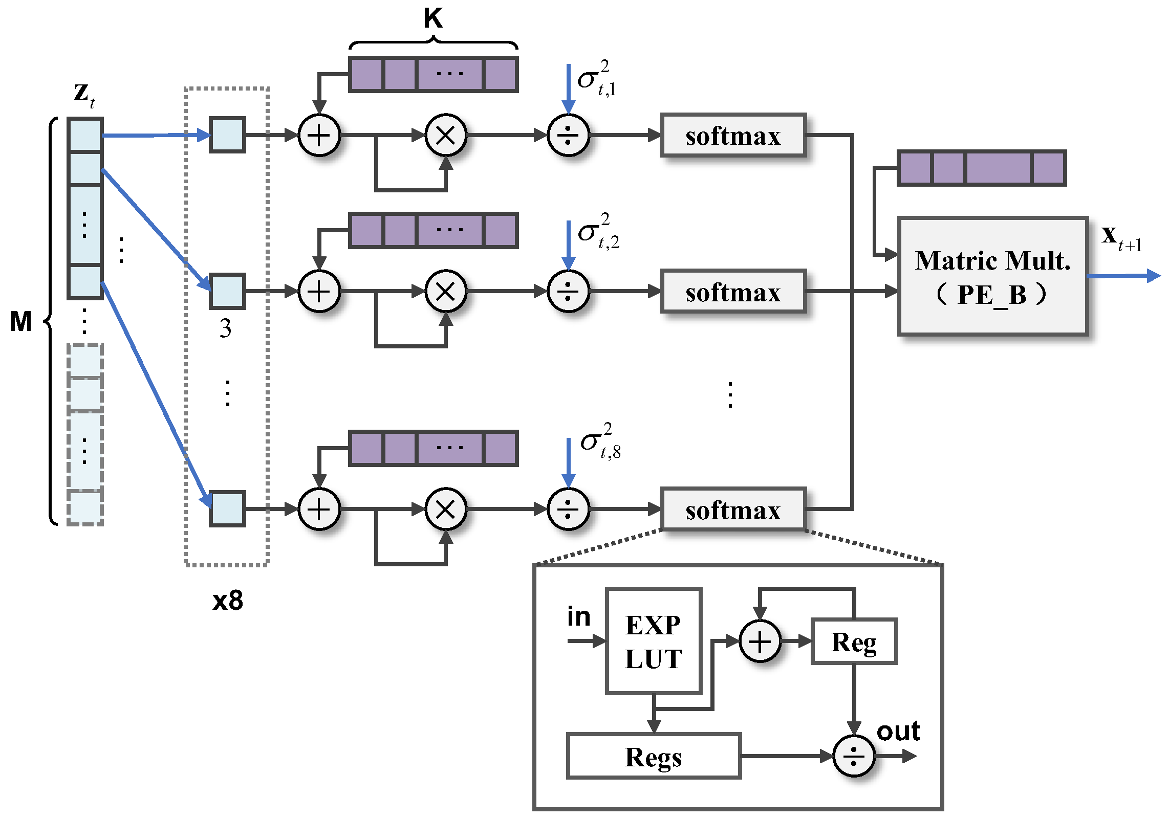
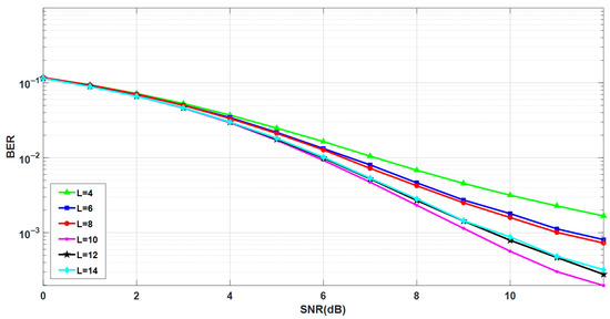
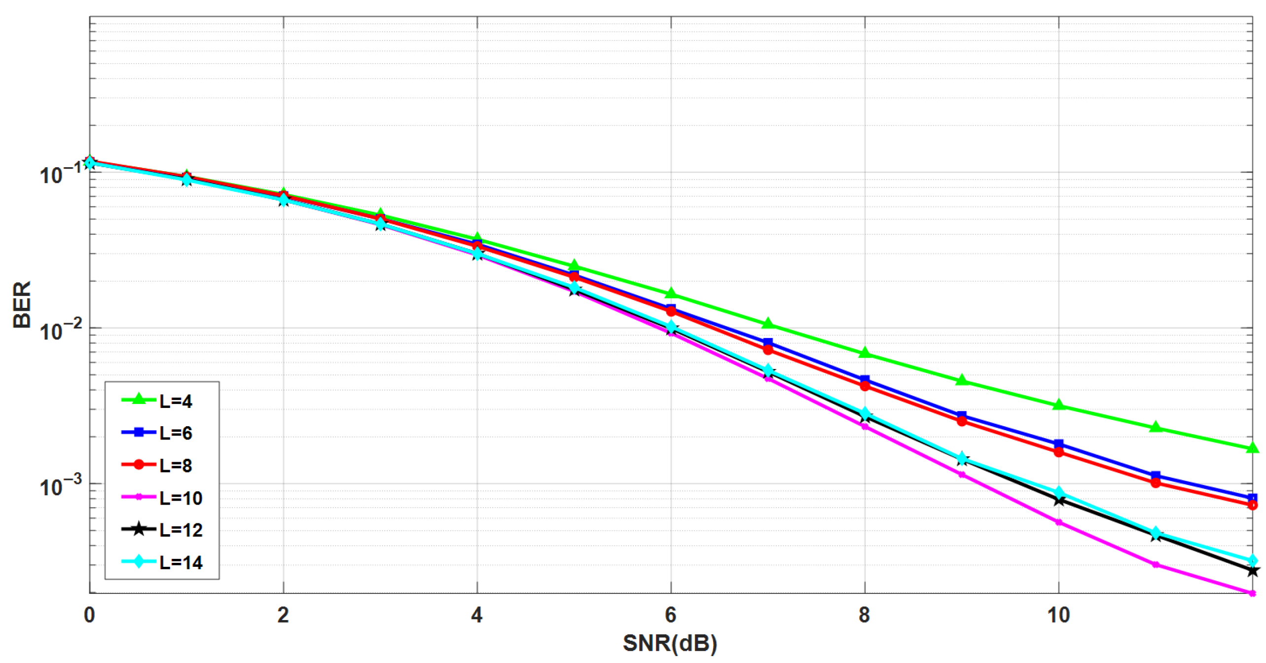
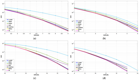
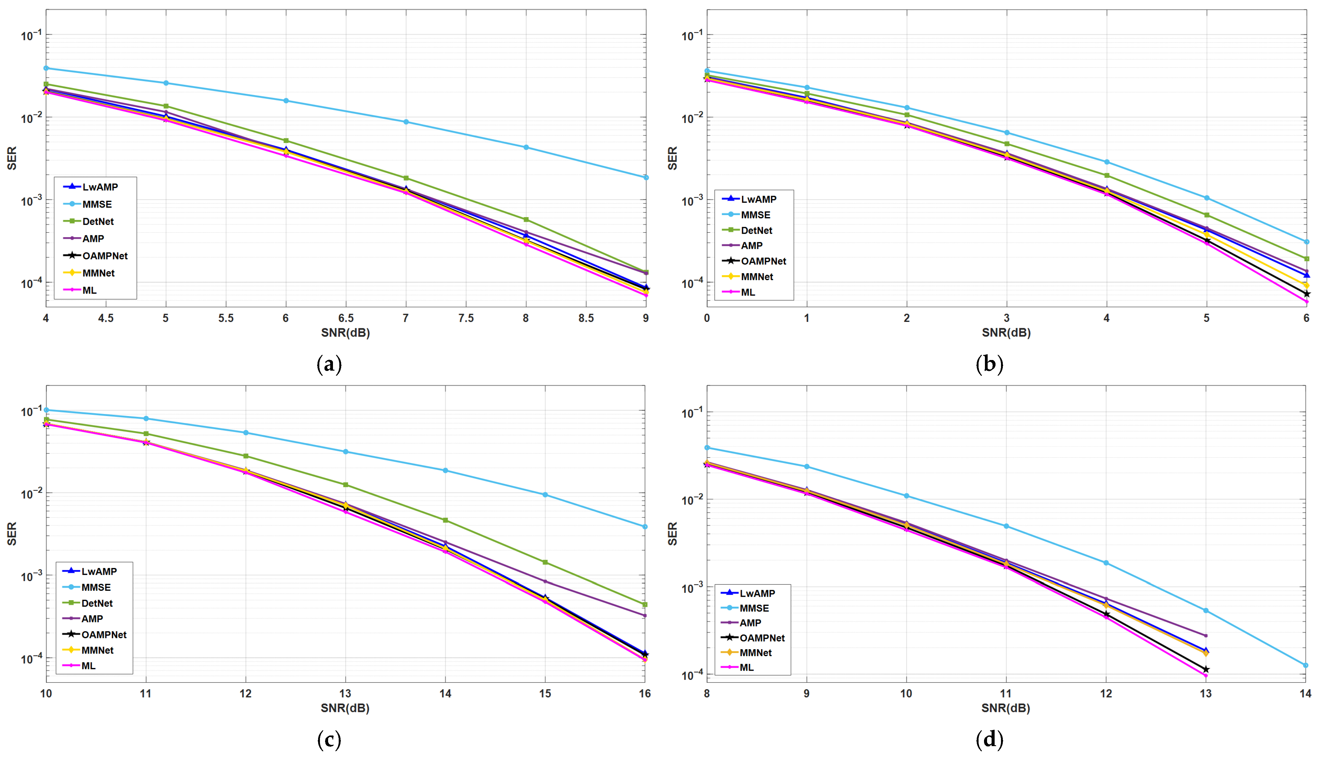
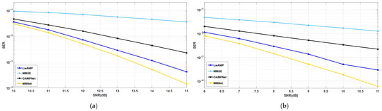
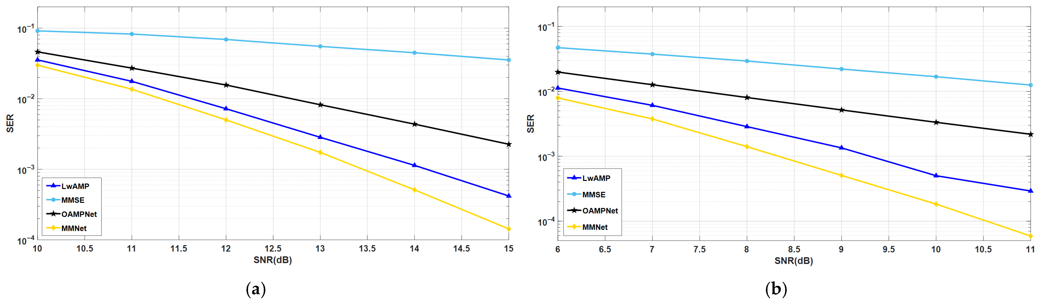

Disclaimer/Publisher’s Note: The statements, opinions and data contained in all publications are solely those of the individual author(s) and contributor(s) and not of MDPI and/or the editor(s). MDPI and/or the editor(s) disclaim responsibility for any injury to people or property resulting from any ideas, methods, instructions or products referred to in the content. |
© 2026 by the authors. Licensee MDPI, Basel, Switzerland. This article is an open access article distributed under the terms and conditions of the Creative Commons Attribution (CC BY) license.