


Featured Application
Generally, for measuring soil moisture and, in particular, for the correct sizing of very low enthalpy geothermal energy facilities.
Abstract
Measuring soil moisture is crucial for optimizing agricultural irrigation, but also, from an energy efficiency standpoint, for the proper design of very-low-enthalpy geothermal energy (VLEGE) facilities. VLEGE represents a renewable energy resource with great potential for residential and industrial applications, as it can provide heating and cooling with high energy efficiency and minimal environmental impact. Soil moisture plays a decisive role in the thermal performance of VLEGE facilities, where small variations in water content can significantly alter the thermal conductivity of the soil and, consequently, the efficiency of their horizontal heat exchangers. This paper presents a low-cost capacitive soil moisture sensor featuring optimized interdigitated electrodes and a controlled dielectric coating that ensures mechanical and electrical stability in subsurface environments. The novelty of this work lies in the validated integration of optimized IDE design, dielectric protection, embedded capacitance acquisition, and gravimetric calibration into a low-cost soil water content measurement device for environmental, agricultural, and VLEGE applications. The developed system converts capacitance variations into direct estimates of soil water content through an integrated microcontroller-based signal-conditioning stage. The developed device is robust, reliable, and readily reproducible. Furthermore, given its low cost (around €50 if manufactured manually; mass-produced it would be much cheaper) and its excellent sensitivity and precision, it is ideal for setting up continuous monitoring networks, even for domestic applications, both in VLEGE installations and in other application domains, such as agriculture and environmental monitoring, where soil moisture measurement is a crucial parameter. This work contributes to the development of more efficient and accessible solutions for harnessing geothermal energy, particularly in installations where dynamic tracking of soil moisture is essential to ensure stable long-term performance.
1. Introduction
From an agricultural standpoint, measuring soil moisture has many applications, such as optimizing irrigation (helping to determine its frequency and duration), efficient resource management (responsible use of water), reducing environmental impact (by reducing fertilizer and nutrient leaching), monitoring the water status of crops, preventing salinity, etc. From an energy efficiency standpoint, measuring soil moisture is essential for the optimal design of very-low-enthalpy geothermal energy (VLEGE) facilities. Since VLEGE accumulates at shallow depths, a few meters below the ground, the facilities to exploit it are usually placed horizontally, taking different forms and always trying to have the largest possible surface area in contact with the ground [1]. The size of these installations, their collectors, is determined by the amount of heat they are capable of exchanging with the ground, which depends on the composition of the soil, its degree of compaction, moisture content, and, of course, depth [1]. The first three variables characterize what is known as the thermal diffusivity of soil, while the last variable, depth, provides the soil temperature, which is well characterized, since its variation curve from the surface to the interior of the soil is generally known and, furthermore, for practical purposes, at a depth of 10 m, the soil is at around the average annual temperature of the surface at that location [1]. Once the soil temperature at the depth where the VLEGE installation is to be carried out is known, the key to designing the installation is to know the thermal diffusivity at that depth, i.e., the speed at which heat spreads through the ground, indicating its ability to conduct thermal energy in relation to its ability to store it [1]. Therefore, for a given soil, thermal diffusivity depends, in practice, on its moisture content, which is why measuring it is so important.
VLEGE is an excellent and renewable way to provide thermal comfort in buildings [2], which can contribute to energy independence and environmental sustainability.
In the study of soil water retention, hygroscopic behavior plays a central role, particularly in fine-textured soils such as silts and clays, whose smaller particle size leads to a larger specific surface area and thus greater water-holding capacity. This larger surface area allows interaction with more water molecules and the retention of significant water volumes. Soil texture [3] is therefore a key factor in water retention. However, water retention does not depend solely on soil particle size; its structure, with stable aggregates and interconnected pores, also influences both the infiltration and storage of water within the soil profile.
As highlighted by [4], a proper understanding of these processes requires consideration of soil composition, which includes primary and secondary minerals and organic matter, and determines the Cation Exchange Capacity (CEC) [5], defined as the surface-area-to-mass ratio of soil particles (m2/g). Specific surface area, mainly associated with soil colloids (clay and organic matter), has a direct effect on water retention: higher specific surface area leads to higher CEC and increased water-holding capacity. This property is not solely controlled by particle-size distribution or soil compaction, which explains its variability among soils. Mineralogical composition, including minerals such as micas and expansive clays, also plays an important role due to their pronounced hygroscopic behavior.
The depth at which soil measurements are taken is another critical aspect [6]. As depth increases, substantial changes occur in the physical and chemical properties of the soil [7]. Surface layers typically contain more organic matter and higher biological activity, which enhance water retention and have important implications for agriculture and forestry. Appropriate selection of sampling depth and rooting depth can improve nutrient uptake and increase crop productivity. At greater depths, however, the presence of specific minerals and higher compaction can lead to denser, less porous structures, reducing infiltration and limiting the availability of water and nutrients to plant roots.
Measurement and calibration of soil water content (SWC) are fundamental for hydrological, climatological, environmental and ecohydrological studies [8]. In hydrology, SWC affects the water cycle by controlling processes such as runoff and infiltration [9], as well as subsurface flows such as interflow [10] and groundwater recharge [11]. In the climate system, SWC is a key variable governing the exchange of water and energy between the land surface and the atmosphere, with a strong influence on evapotranspiration [12].
Understanding the temporal and spatial behavior of SWC is therefore essential for a wide range of investigations. Although several methods exist for measuring soil moisture, gravimetric analysis and oven-drying [13] remain reference techniques due to their simplicity, directness and accuracy. However, they are laborious and slow, which makes them unsuitable for real-time continuous monitoring.
To overcome these limitations, SWC can be inferred from the dielectric constant [14], an electrical property related to the ability of the soil to store and transmit electrical energy. Accurate measurement of this property enables reliable estimation of soil moisture, which is crucial for assessing water availability for plants, understanding hydrological behavior and supporting the design of VLEGE systems.
In this context, capacitive sensors [15] have been proposed as an effective alternative for SWC measurement. These devices operate through an electrical circuit that detects changes in capacitance C of the surrounding medium, which are directly related to variations in its dielectric constant. As a result, capacitive sensors are widely used for soil water monitoring [16], which is particularly important in VLEGE applications where soil moisture controls steady-state heat transfer in porous media [17]. This property is influenced by multiple factors, including degree of saturation, dry density, soil mineralogy, particle size and effective soil volume [18,19,20]. In this sense, soil water content not only affects hydraulic and dielectric properties but also plays a key role in the efficiency of geothermal heat exchangers [21].
Recent literature confirms that capacitive soil moisture sensing remains an active research field, particularly for low-cost environmental monitoring applications. For example, [16] evaluated the performance of capacitive soil moisture sensors under field conditions, highlighting the influence of soil properties and environmental variability on sensor response. Similarly, [22] proposed an integrated capacitive sensing platform for rapid soil moisture detection in field environments. These studies demonstrate the relevance of capacitance-based sensing approaches while also indicating the need for robust, low-cost devices capable of operating reliably in real soil conditions. More specifically, recent work has confirmed the continued interest in interdigitated-electrode (IDE)-based capacitive architectures for soil-moisture sensing, while analytical studies have shown that IDE capacitance is strongly affected by electrode geometry, multilayer dielectric structure, and surrounding media [22,23].
In addition, recent calibration studies on low-cost capacitive soil moisture sensors have highlighted that acceptable accuracy can be achieved only after appropriate sensor-specific or batch-specific calibration, and that comparison with commercial or reference instruments remains essential to position a new design in terms of cost, accuracy, and applicability [24]. For this reason, the present manuscript explicitly addresses not only sensor design, but also practical calibration, repeatability, and the intended deployment context.
The novelty of this work does not lie in the generic use of capacitive sensing or IDE topologies, both of which are well established in the literature [16,22], but in the development and validation of a buried, low-cost, field-deployable soil water content (SWC) sensing system that combines: (i) an IDE geometry designed to maximize the practical dynamic capacitance range between dry and saturated soil conditions, (ii) a controlled dielectric protection strategy suitable for subsurface operation, (iii) an integrated microcontroller-based signal-conditioning stage for direct capacitance acquisition, (iv) a gravimetric calibration campaign conducted under controlled conditions, and (v) an application-oriented analysis focused on environmental monitoring, irrigation support, and VLEGE systems.
The resulting device is particularly suitable for field studies and resource-constrained environments, such as small-scale agricultural settings [25,26,27,28,29,30] and domestic VLEGE heat-exchange installations [31,32,33,34], where a dense network of low-cost sensors may be preferable to a limited number of high-cost instruments.
To make this contribution explicit, the manuscript first presents the physical basis of capacitance-based SWC measurement and its practical limitations, then details the sensor geometry, protection strategy, and conditioning electronics, and finally reports the gravimetric calibration procedure, the repeatability observed among professionally manufactured sensors, and the implications of the proposed device for distributed monitoring and VLEGE applications.
2. Materials and Methods
2.1. Theoretical Foundations
As is well known, dielectric permittivity (ε) measures a material’s ability to become polarized in the presence of an electric field. The permittivity of vacuum (ε0) is a physical constant with an approximate value of 8.854 × 10⁻¹² F/m, which is used as a baseline permittivity, so that for any material, its relative permittivity (εr) is used, that is, its permittivity with respect to that of a vacuum: εr = ε/ε0. Permittivity is related to capacitance in capacitors, where high permittivity allows more charge to be stored [35]. Figure 1 shows a capacitor in its simplest form. It is a flat capacitor, consisting of two parallel plates of area A separated by a distance L and filled with a dielectric characterized by its permittivity ε. The capacitance of an ideal flat capacitor (perfectly aligned parallel plates and homogeneous dielectric) is given by Equation (1).
Figure 1.
(a) Schematic of ideal flat capacitor filled with homogeneous medium. (b) Equivalent circuit.
The capacitance of soil to store electrical charge can be described by a capacitor model (the circuit in Figure 1 is used only as an approximation) in which the amount of stored charge depends on the applied potential difference and the dielectric properties of the soil in which the potential difference is applied. Taking Equation (1) into account, for given condenser dimensions, the capacitance of soil will be significantly influenced by its permittivity, which will depend fundamentally on its composition, density, and presence of water [36].
When analyzing the behavior of dielectric materials under time-varying electric fields, it can be observed that the relative permittivity is a complex quantity (2), whose imaginary part , known as the loss factor, measures the amount of energy that the material dissipates in the form of heat due to the friction of molecular dipoles as they attempt to follow the electric field, while its real part represents the material’s capacity to store electrical energy through polarization [37]. εr is not a fixed constant, but varies with the frequency (ω) of the applied field [38].
According to [39], the relationship between capacitance (C), resistance (R), and relative permittivity at angular frequency ω for a flat capacitor such as the one in Figure 1 can be expressed as (3) and (4).
The ratio between and known as the loss tangent (tan δ), is expressed by Equation (5).
By solving and from (3) and (4), respectively, the loss tangent is obtained by (6).
In principle, because L and A cancel out in (5), the measurement of tan δ in parallel-plate capacitors would appear to be independent of geometry. However, ref. [40] demonstrated that is only an idealization, since the presence of blocking layers in the plates introduces an additional capacitance in series (Figure 2). This boundary layer capacitance depends directly on the plate separation L, thereby influencing the tan δ measurements and making them geometry-dependent, and for this reason, other optimized geometries are used, as is done in this work.
Figure 2.
Equivalent circuit that includes blocking layers.
In Figure 2, is the capacitance associated with the blocking layers with a thickness of 2bl.
Considering this additional capacitance and the fact that, as reported in several studies [8,41], the imaginary part of is employed to estimate soil water content, it can be stated that the electrical conductivity (σ) is the only contribution to that can be expressed by (7).
In this expression, denotes the loss due to dielectric relaxation.
In summary, analyzing Equations (3) and (4), a high permittivity of the soil indicates a high water content. This is because water has a large (≈80.4 at 25 °C), as water molecules are interconnected through hydrogen bonds (H-bonds) [42,43]. As a result, capacitance in (3) increases or resistance in (4) decreases.
Soil permittivity is a complex dielectric parameter, as its composition (mixture of solids, water, and air) varies even in nearby soil portions. However, moisture will always be the dominant factor, since for water ≈ 80.4, whereas for air and solids it ranges between 1 and 5. Based on this and in accordance with [44], the estimation of volumetric water content () from capacitance is justified by the proportionality between C and the permittivity of the soil, which is usually referred to as the effective permittivity of the soil . Thus, an optimized measurement of C (the focus of this work) allows to be derived, which is then used to calculate using Equation (8). Therefore, the chained relationship constitutes the physical basis for estimating soil moisture from capacitance measurements.
It is important to note that the relationship in Equation (8) is empirical and was derived for mineral soils with low salinity. Although the physical basis of capacitance-based SWC sensing is well established, the practical response of a buried capacitive sensor is affected by several factors beyond moisture alone. Previous studies have shown that soil-dependent behavior remains relevant even for integrated capacitive devices, since the response may vary with soil group, material selection, and device-specific calibration conditions [22]. Likewise, field-oriented studies on capacitive sensors based on Printed Circuit Board (PCB) have highlighted the need for local calibration and careful interpretation of sensor output under real environmental conditions [16]. Therefore, soil texture, mineral composition, temperature, salinity, electrical conductivity, and encapsulation layers should all be regarded as factors capable of modifying the effective dielectric environment sensed by the capacitive sensor [16,45].
For this reason, the capacitance-to-SWC relationship should not be interpreted as universal. Instead, it must be obtained through calibration for the specific sensor architecture and, ideally, for the soil and environmental conditions of interest, as also emphasized in recent studies on low-cost capacitive sensing [24].
According to the study conducted so far, there is a clear correlation between the capacitance of a capacitor that uses soil as a dielectric and the moisture it contains. From this point onwards, in order to measure this moisture, it is important to manufacture a device that has a wide range of capacitance variation between zero moisture (absolutely dry air or soil) and maximum moisture (water or waterlogged soil). As is well known, to achieve greater capacity in a capacitor connection, the capacitors must be connected in parallel. This is the principle behind the design known as interdigitated electrodes (IDE).
Interdigital capacitors (IDEs) are quasi-planar devices consisting of interdigitated metallic electrodes arranged in a comb-like geometry on a dielectric substrate (Figure 3). This structure generates a fringing electric field, enabling high sensitivity to variations in the permittivity of surrounding materials. Since the 1970s, IDEs have been widely applied in microwave systems, dielectric characterization, and material sensing, providing a compact and accurate alternative to conventional capacitors [23].
Figure 3.
Schematic representation of an interdigital capacitor (IDE) consisting of two interdigitated metallic electrodes (Electrode A and Electrode B) arranged in a comb-like geometry on a dielectric substrate.
Capacitance can be significantly enhanced through electrode geometry optimization, facilitating the development of high-sensitivity thin-film sensors [46]. IDEs fabricated via DC magnetron sputtering have also proven effective for measuring the permittivity of crude oil, highlighting their relevance in industrial monitoring and characterization of complex materials [47]. In addition, the use of anisotropic coatings, such as nematic liquid crystals, has extended their application to high-precision electromagnetic sensing [48].
Recent advances include the integration of IDEs on flexible substrates, enabling new device architectures such as capacitive tactile sensors adaptable to various industrial environments [49]. While predominantly used in industry, IDEs also show potential in agricultural applications, particularly for the dielectric characterization of soils and biomaterials. In this context, their capacitance is particularly sensitive to variations in the permittivity in soil media, making them well suited for soil moisture sensing. These devices typically operate within a frequency range from 10 Hz to 100 kHz, and their calibration depends on key geometric parameters such as electrode spacing and area.
The capacitance of an IDE sensor, such as the one shown in Figure 3, can be expressed by Equation (9) [46,47,48]:
where n is the number of electrodes, H, w, and t denote the effective length, width, and thickness of the electrode, respectively, while L represents the spacing between them. In addition, ε0 the permittivity of vacuum (8.854 × 10⁻¹² F/m), εr is the relative permittivity of the surrounding medium, and εs is that of the substrate on which the electrodes are placed. The function K(x) corresponds to the complete elliptic integral of the first kind evaluated at x.
The first term in Equation (9) describes the capacitive contribution associated with the coplanar configuration of the electrodes, i.e., the coupling due to the fringing field. The second term (2εrt/L) represents the contribution analogous to a parallel-plate capacitor, accounting for the electrode thickness; in practice, this term is generally negligible compared to the first in this type of structure.
In practical terms, and focusing on the objective of this work, IDE geometry can be used to maximize sensitivity and dynamic range; however, the resulting sensor must still be experimentally characterized and calibrated under controlled conditions before being used as a quantitative SWC measuring device.
2.2. Equipment and Materials Used
This research work involves a large number of measurements, data acquisition, sensor conditioning, and calibration procedures, requiring the use of various instruments and equipment, which are summarized in Table 1. All the equipment listed in Table 1 is professional and commercial grade, meaning it has been tested, calibrated, and guarantees quality and reliability in use, so it can be used as a reference for the performance of the developed sensor. Throughout this document and following the order in Table 1, they will be referred to as capacitance meter, precision balance, moisture meter, controlled oven, and load cell. Table 1 also lists the characteristics of the resin used (referred to in the text as epoxy resin) to coat the sensors developed.
Table 1.
Equipment used in all tasks performed.
3. Results
3.1. Sensor Development
Based on the previous theoretical considerations, the sensor prototypes were developed and experimentally evaluated. The operating principle of the proposed sensor is based on the dielectric interaction between the electric field generated by the electrodes and the porous soil medium, whose effective permittivity depends on the volumetric fractions of water, air, and minerals. In this context, the capacitance C can be expressed in general terms according to Equation (9), where the relationship among its geometric parameters provides the physical basis for the proposed sensor design.
Numerous prototypes with different shapes and configurations were developed in our laboratory. Figure 4a illustrates the geometric disparities between some of the developed sensors, revealing limitations present in certain designs, particularly the lack of a sufficiently large contacting surface between electrodes. This deficiency affected the distribution of the electric field within the soil and compromised the accuracy of moisture measurements. Nevertheless, the less efficient designs were essential for identifying the best configuration developed in this work, which is shown in Figure 4b. This chosen sensor, selected after multiple empirical tests, was fabricated in our laboratory using photolithographic techniques to obtain the PCB.
Figure 4.
(a) Different sensors developed; (b) Selected sensor.
From a design standpoint, the selected geometry was not chosen arbitrarily. Electrode width, spacing, number of fingers, and active length were progressively refined in order to maximize the effective interaction volume between the fringing electric field and the surrounding soil while preserving mechanical robustness of the PCB and manufacturability with standard photolithographic processes. In particular, the 0.75 mm spacing was adopted as a compromise between higher sensitivity, reduced risk of manufacturing defects, and sufficient dielectric penetration into the porous medium. The final layout therefore reflects an optimization strategy focused on enhancing the sensor response to soil moisture variations under practical subsurface conditions, while maintaining fabrication feasibility and structural robustness, rather than merely maximizing nominal capacitance from geometric considerations alone.
Figure 4b shows an IDE capacitor geometry that provides effective coupling with the surrounding dielectric medium, increasing the sensor’s sensitivity to changes in soil moisture [50]. In addition, the tapered end of the design facilitates its natural insertion into the soil, without the need for specialized tools.
The design of the selected sensor, shown in Figure 4b, is presented in detail in Figure 5. It consists of 76 copper electrodes 1 mm wide and 32.5 mm long, separated by 0.75 mm. The thickness of the copper electrodes is 35 μm.
Figure 5.
Detailed geometry of the selected sensor. All dimensions are given in mm.
For calculation purposes, an effective electrode length of 33.5 mm was adopted. This is because each electrode forms an additional capacitor with a plate length of 1 mm, alternating with one of the copper tracks that runs across the entire substrate. See the area highlighted in blue in Figure 5 as an example.
Thus, with the above parameters, the IDE capacitance based on Equation (9) yields by Equation (10).
Using three reference media with markedly different dielectric constants: dry air (, water () and isopropyl alcohol C3H8O (), respectively, the theoretical capacitance values shown in Table 2 are obtained using (10).
Table 2.
Theoretical capacitance values of the sensor in the three-dielectric media (air, isopropyl alcohol and water), by applying (10) for εs = 4.5 and εs = εr.
Table 2 provides the theoretical capacitance values for the cases εs = 4.5 and εs = εr. In the developed device, the substrate on which the electrodes are deposited consists of a thin 1.6 mm FR-4 sheet, with a typical relative dielectric constant of εs = 4.5. As will be described later, our experimental procedure involved immersing the sensor in different media. Under these conditions, the actual substrate can be considered as composed of two materials: the thin FR-4 sheet and the test medium itself, whose influence may be predominant due to its larger volume. For this reason, it seems reasonable to present both reference values.
Five identical sensors (prototypes 2001–2005) were manufactured in our laboratory (Figure 6) in order to evaluate both the suitability of the design and its repeatability in measurement, bearing in mind, however, that the manual manufacturing process may lead to variations in results, even in sensors with nominally identical dimensions, due to differences in development time or exposure to the chemical etcher.
Figure 6.
Image of the five manually manufactured capacitive soil moisture sensors (prototypes 2.001–2.005).
To compare the theoretical capacitances of Table 2, the capacity of the five IDE sensors developed was measured using the capacitance meter (Table 1) in the same three different media (dry air, isopropyl alcohol and water), as shown in Figure 7.
Figure 7.
Characterization of the capacitive soil moisture sensor in: (a) air, (b) isopropyl alcohol and (c) water.
Theoretically speaking, based on Equation (10), the five sensors manufactured should have the same capacity when measuring in the same medium. However, in practice, as will be seen, although they are similar, they are not exactly the same. This can be verified in Table 3. There is a clear difference in capacitance between the three media tested, confirming the proper functioning of the 5 sensors and their sensitivity to the dielectric properties of the three different fluids.
Table 3.
Capacitance values of the 5 manually manufactured sensors in the three-dielectric media (dry air, isopropyl alcohol and water).
Table 3 shows that a baseline capacitance (minimum possible capacity) was obtained in the dry air. This measurement serves as a reference for evaluating the sensitivity of the sensor when the dielectric is a different medium. Thus, when the sensor was immersed in water, a pronounced increase in capacitance was observed, attributable to the high of water (approximately 80.4 at 25 °C), which leads to greater charge accumulation between the electrodes. The ratio in Table 3 provides a direct indication of the sensor’s sensitivity to media with high permittivity. The capacitance measured in isopropyl alcohol was intermediate between that of air and water, which is consistent with its dielectric constant (approximately 19.9 at 25 °C), considerably lower than that of water but much higher than that of air. In this case, the ratio is .
The comparison between the theoretical capacitance values for εs = εr (Table 2) and the average of the measured values reported in Table 3 is presented in Table 4, where reasonably acceptable differences (between 3% and 15%, with respect to column II, which demonstrates that when they are submerged in the medium, εs = εr) taking into account that Equation (10) corresponds to a purely theoretical model with a certain degree of idealization. In practice, it is difficult to ensure both dimensional accuracy and material homogeneity in IDE devices, especially when they are fabricated using photolithographic processes with chemical etching.
Thus, the main design criterion was not the maximization of analytically predicted capacitance itself, but rather the attainment of a sufficiently wide experimental dynamic range that could be maintained after the incorporation of the protective layers required for buried operation. This approach guided the progressive refinement of the sensor, from manually fabricated prototypes to the final professionally manufactured and encapsulated version intended for field deployment.
These initial results confirm the proper functioning of the designed capacitive sensor type and its ability to discriminate between media with different dielectric properties. However, outside the laboratory, direct and prolonged exposure of the device to harsh conditions, such as high moisture, thermal fluctuations, dissolved salts and aggressive chemicals naturally present in soils, as occurs in agricultural or geothermal applications, can cause both physical and electrochemical degradation processes that severely compromise measurement accuracy or even the integrity of the sensor itself [51]. For this reason, resin encapsulation emerges as an effective strategy for enhancing the durability and electrical stability of the developed sensors [52]. After considering several encapsulation options for the moisture sensor, and in light of the findings reported in [53], a polyester resin was initially selected. This option was later discarded, since it was observed that it absorbed moisture, had poor adhesion to the PCB during curing, and even caused board deformation. From that point on, different epoxy resins were evaluated as encapsulation alternatives. In particular, DECOART® epoxy resin (referred to simply as “epoxy resin” in the rest of the article) was employed due to its thermosetting structure, as indicated in its technical datasheet [54]. It also acts as a highly effective dielectric and chemical barrier, significantly reducing water permeability and limiting the diffusion of potentially corrosive ions to sensitive areas of the circuit.
As expected, epoxy encapsulation affects the sensitivity of the sensor to changes in moisture, decreasing it as the coating thickness increases. Table 5 shows this effect for three of the five developed sensors (2.002, 2.003 and 2.004), for which different epoxy-resin deposits were applied. In the revised analysis, the encapsulation layer is described in terms of coating thickness, since this parameter is more appropriate than mass for discussing its influence on dielectric behavior and sensor response. The coating thicknesses considered for sensors 2.002, 2.003 and 2.004 were 1.44 mm, 0.76 mm and 0.30 mm, respectively. Tests were carried out (Figure 8) until the minimum coating that still provided adequate protection was reached; under these experimental conditions, this lower bound corresponded to approximately 0.30 mm (about 4 g of resin). Lower thicknesses produced a very thin layer that could easily deteriorate with minimal friction.
Table 5.
Capacitance values of the sensor for models Sensor 2.002, Sensor 2.003 and Sensor 2.004 depending on the weight of epoxy resin uniformly deposited: 20, 10 and 4 g.
Figure 8.
Sensors used in the encapsulation-thickness study: (a) Model 2.002, coating thickness of 1.44 mm (20.28 g of resin); (b) Model 2.003, coating thickness of 0.76 mm (10.74 g of resin); (c) Model 2.004, coating thickness of 0.30 mm (4.17 g of resin).
The 2.002 model sensor in Figure 8a, which incorporated the largest coating thickness (1.44 mm), exhibited an almost negligible response to variations in soil moisture (), indicating a detrimental effect on its performance. Sensor model 2.003, Figure 8b, with an intermediate coating thickness of 0.76 mm, showed a similar response despite the reduction (), suggesting that even this amount remains excessive and has a very negative effect on the sensitivity of the sensor. In contrast, sensor model 2.004, Figure 8c, with a coating thickness of 0.30 mm, showed sensitivity () that could be considered acceptable. An example of the measurements taken with the capacitance meter is shown in Figure 9.
Figure 9.
Model sensor 2.004: (a) Tests in dry air. (b) Tests in water.
Having achieved the best performance in the laboratory with manual procedures, the next phase of sensor development consisted of giving it a professional finish and quality. To this end, a specialized company was commissioned to manufacture 5 sensors similar to those developed in the laboratory (those shown so far in the article). These sensors are factory-coated with a layer of aliphatic epoxy resin (AER), as shown in Figure 10, in order to provide high resistance to weathering and prevent electrochemical migration (ECM), as indicated in [55]. The price to pay for incorporating this protective coating into the sensor is the introduction of a new dielectric into the electric field of the IDE, which modifies the total capacitance of the sensor. This is influenced by the of the AER, which ranges from 3.3 to 4.6, and the thickness of the AER coating, which is approximately 25 μm.
Figure 10.
Capacitive soil moisture sensors manufactured by a professional PCB company and coated with AER (green resin in the figure). Designed as 3.001 to 3.005.
Once again, professionally manufactured sensors were measured in the same media as in the previous section, using the capacitance meter (Figure 11). The results are presented in Table 6.
Figure 11.
Characterization of the professionally manufactured and factory-coated capacitive soil moisture sensor with AER in: (a) dry air, (b) isopropyl alcohol and (c) water.
Table 6.
Capacitance values of the sensors coated with AER in the three-dielectric media (dry air, isopropyl alcohol and water).
Although the AER coating provides protection against adverse environmental conditions, the sensor is subject to friction from sand, stones, etc., in the soil; therefore, this protection is not sufficient, as its deterioration can lead to corrosion of the conductive tracks, compromising the long-term proper functioning of the sensor. For this reason, an additional encapsulation layer was implemented to protect the sensor from the environment, which has proven to offer adequate protection in adverse conditions [56]. The same epoxy resin used in the laboratory prototype was used for this purpose. In this regard, it is important to note that, as indicated in [57], this epoxy resin affects the dielectric behavior of the medium, since its , as stated in its datasheet [54]. However, since the sensor comes factory-coated with AER (Figure 10), the additional protective coating with epoxy resin does not need to be as thick as in the previous experiment on sensors manufactured by the authors (Figure 8); thus, an additional epoxy layer with a coating thickness of 0.11 mm (corresponding to 1.54 g of resin; Figure 12) was used, compared with the previously tested manual coating thickness of 0.30 mm (4.17 g). This results in a less pronounced detrimental effect on the effective dielectric constant, allowing for greater interaction between the sensor and the surrounding moisture.
Figure 12.
Professionally manufactured sensor with a factory-applied AER layer and an additional manually deposited epoxy coating with a thickness of 0.11 mm (1.54 g of resin).
Once again, the tests were repeated by measuring the capacitance with the capacitance meter. To determine the measurement range, the two extreme dielectric media (dry air and water) were used. The results are shown in Table 7. Table shows a comparison of the results obtained in all the experiments carried out. In it, the first three sensors represent the one manufactured manually (Figure 6) with the epoxy resin added, also manually, in the laboratory (Figure 8 and Table 5). The following five sensors represent those manufactured professionally as they leave the factory, i.e., only with AER (Figure 10 and Table 6). The last three sensors represent the final design, i.e., the professional sensor with factory-added AER (Figure 10) plus the manual addition of epoxy resin in the laboratory (Figure 12). To do this, only three of the five available sensors (3.001 to 3.005) were used: 3.002, 3.003, and 3.004 These sensors with the added epoxy resin were finally named sensor 1, sensor 2, and sensor 3, respectively. In this regard, it should be noted that other sensors could have been used, or even just one of the five, as the variations between them are minimal. Note that any of the three sensors considered as final developments have an excellent dynamic range, close to 1600 pF, for a minimum measurement close to 200 pF and a maximum close to 1800 pF.
Table 7.
Capacitance values of manually and professionally manufactured sensors.
The measurements summarized in Table 7 also help define the role of the LCR meter within the overall validation workflow of the present study. In particular, the LCR meter was used as a reference instrument during the sensor-development stage to establish the physical capacitive response of the device under controlled dielectric conditions and to verify the dynamic range of the final protected architecture. Once this reference capacitance range had been established, the next stage focused on the implementation of a low-cost embedded acquisition system intended not as a replacement for laboratory instrumentation, but as a practical measurement solution for calibrated soil-moisture monitoring.
3.2. Signal Conditioning System
After experimentally validating the behavior of the designed sensor in different media and confirming its sensitivity to dielectric variations in the surrounding environment, the next step in developing the measuring device was to implement a system for conditioning the signal provided by the sensor. It must provide reliable operation in real-field conditions, converting capacitance variations into a stable and linear electrical quantity that is resistant to noise, thermal drift, and electromagnetic interference [58]. This process is essential to ensure that measurements obtained in the field maintain the accuracy observed in laboratory settings, allowing the device to be integrated into continuous monitoring systems and definitively validated under real operating conditions.
To condition the capacitive sensor signal, a microcontroller from Microchip Technology’s SAM family (Microchip Technology Inc., Chandler, AZ, USA), a series of 32-bit ARM® Cortex®-M microcontrollers, was chosen because it is designed for a wide range of applications and these devices offer high performance, low power consumption, and a wide range of peripherals [59]. Specifically, the microcontroller chosen was the ATSAM3S1AA-MU from Atmel (Microchip Technology Inc., Chandler, AZ, USA) [60]. Capacitance measurement with the microcontroller is based on determining the charging time at a known voltage and converting it into capacitance. While this approach is straightforward when a capacitor is charged through a known resistance, it becomes more complex in the present case because the relevant resistances are not precisely known and additional capacitances are only approximately known. In particular, the internal configuration of any analog pin of the selected microcontroller must be taken into account (Figure 13). One factor limiting measurement accuracy is the uncertainty in the internal pin capacitance, which is not specified as a fixed value by the manufacturer and may range between 20 and 30 pF. This effect must therefore be compensated through calibration.
Figure 13.
I/O pin equivalent schematic.
Using two analog pins on the microcontroller, for example A0 and A1, the circuit diagram with the capacitive sensor connected, , is shown in Figure 14a. As for the connection of and , if pin A1 is configured as a source (5 V), the equivalent circuit during the charging transient is shown in Figure 14b, where pin A0 will provide the reading and then, by setting it to low, serve as a discharge circuit for , thus enabling a new measurement cycle to begin.
Figure 14.
(a) Connection of the sensor under study to the ATSAM3S1AA-MU microcontroller. (b) Equivalent circuit formed by the sensor and the internal capacitor of the microcontroller.
Once and are charged, will be a stable voltage independent of time. Solving Equation (12) for taking this into account, yields (13).
Equation (13) allows to easily obtain the value measured by the sensor, , since if the output voltage of A1 is +5 V, its value in the microcontroller’s ADC converter, which has 10 bits, will be , so it is only necessary to know the value of the reading in A0 at the end of the charging process. However, there is a problem that seriously affects the accuracy of the measurement, and that is the uncertainty of the value. To overcome this, it is necessary to calibrate each pin used in each chip. The way to do this will be illustrated with an example carried out in the laboratory:
- Use a commercial capacitor, , with a value comparable to . A 100 pF was used;
- Measure the actual capacitance with a professional meter. The measured value was 104 pF;
- Make the connection shown in Figure 14a, replacing with ;
- Activate the charging process shown in Figure 14b. The value of the ADC microcontroller reading for was 803;
- Finally, solving (13) for with instead of , gives (14).
By substituting into Equation (13) the value of calculated in (14), it is possible to obtain an accurate measurement of and, therefore, of the measured capacitance of the soil.
3.3. Sensor Calibration
At this point, the sensor has been fully designed, along with its conditioning circuit (Figure 15). This sensor, its capacitance, has been experimentally proven to be highly sensitive to dielectric changes, which are mainly caused by the amount of water (moisture) in the soil where they are buried. Therefore, since the aim is to measure moisture with the sensor, the next step is to correlate changes in its capacitance with moisture, which will allow the sensor to be calibrated.
Figure 15.
Capacitive moisture sensor with its signal conditioning channel: (a) top view, (b) rear view.
The sensor was calibrated by means of a gravimetric procedure, chosen because it provides a direct and accurate reference for soil water content. This choice is also consistent with recent studies on low-cost capacitive soil moisture sensing, where gravimetric measurements have been used as the reference basis for deriving calibration equations under local soil conditions [16,34]. For reproducibility, the calibration protocol followed the sequence below: (i) a representative soil sample was placed in a PVC test tube with the sensor fully buried in the soil volume; (ii) the soil was brought to its upper moisture endpoint under controlled conditions, and the corresponding initial mass was recorded; (iii) the test tube was progressively dried in a controlled oven until the lower moisture endpoint was reached and the final mass was obtained; (iv) during the complete drying process, simultaneous capacitance and mass measurements were acquired so that each capacitance value could be associated with a gravimetrically derived moisture value; and (v) the resulting capacitance–moisture dataset was then used to fit the calibration model reported later in this section.
For the calibration process, a soil type classified as cambisol was used, characterized by being a sandy clay soil with a very deep C horizon [61]. This is the typical soil in the area surrounding the Research Center where the authors work: Center for Research in Technology, Energy, and Sustainability; its acronym in Spanish is CITES and is located in Huelva, in southwestern Spain. The present calibration should therefore be interpreted as representative of this soil type and not as a universal transfer function for all soils.
Three test tubes made of PVC (polyvinyl chloride) were used for the calibration process. The test tubes are pieces of pipe filled with the type of soil used. Each sensor was completely buried in one of the test tubes. A load cell was used to monitor the wet weight and dry weight of each test tube [62]. The assembly was placed inside the controlled oven (Figure 16).
Figure 16.
Test tubes on top of load cells with buried sensors, all inserted into the controlled oven.
Since the calibration process consisted of correlating the capacitance sensor from the minimum moisture value (dry soil) to maximum moisture value (saturated soil), the moisture meter (Table 1) was used to ensure both calibration endpoints. Figure 17 shows the insertion of the moisture meter into the test tube. Of course, the moisture meter was weighed using the precision balance and its weight was subtracted from the weight of the soil in the test probe.
Figure 17.
Moisture meter inserted into the test tube to ensure the two calibration endpoints.
In order to simulate actual soil conditions, the controlled oven was programmed to operate at a constant temperature of 30 °C (a typical soil rarely reaches a higher temperature), even at the cost of having to set the duration of the experiment (from moisture-saturated soil to dry soil) for 12 days.
Figure 18 shows the block diagram of the instrumentation system used to record the test data. The instrumentation system was designed to take simultaneous capacitance samples (from the sensors developed) via a ModBus communications system, together with weight samples (amount of water and, therefore, humidity) from the test tubes via the load cells. Capacitance and weight samples were taken every 30 s for 12 days (34,560 samples).
Figure 18.
Instrumentation system to record the test data.
Between 14 and 26 February 2025, an initial test was conducted to evaluate the quality of the measurements. Figure 19 shows the results of the capacitance measurements from saturated wet soil to dry soil. Each of the three test tubes was brought to maximum moisture, as indicated by the moisture meter, which meant that the moisture sensors developed were giving their maximum value. From there, the test tubes were left to dry in the controlled oven at a stable temperature of 30 °C until the moisture meter indicated that all the water had disappeared from the test tubes and that, therefore, the moisture sensors developed were giving their minimum value. Figure 19 shows that, as expected, the behavior of the three sensors in response to moisture is practically identical. This can be seen in Table 7, where there are only a few picofarads in the ΔC of each sensor. Figure 19 also shows that there is a considerable amount of noise in the measurements. In order to mitigate this noise between samples, a second test was carried out in which 100 measurements were taken for each sample, taking the average of the 100 as the measured value. This measurement procedure virtually eliminated noise between samples and showed that, in practice, the measurements from the three sensors overlapped. From this, it was concluded that it was not necessary to carry out a calibration process for each sensor, as it was sufficient to carry it out on one of them and apply it to the entire series of sensors manufactured (Figure 10). Figure 20 shows the results of this second test conducted between 15 and 25 March 2025. Figure 20 shows the capacity measurements of sensor 1 (as explained above, it is now referred to simply as “sensor”) together with the weight measurements of the test tube in which it is buried. Note that now the difference between capacities and weights measured in each sampling produces a smooth function. This is because, despite the high sensitivity of the sensors, such frequent sampling (every 30 s) and average measurements (over 100 captures each time) completely mask the noise.
Figure 19.
Capacitance behavior of sensors over a complete cycle of moisture variation.
Figure 20.
Sensor capacitance and test tube weight during a complete moisture variation cycle.
Based on the weight data of the test tube, the percentage of volumetric water content () is obtained immediately and directly by means of (15).
where is the weight of the test tube sample, the weight of the test tube without any water and the weight of the test tube saturated with water. Therefore, taking into account that the values of the measurements taken were and , the relationship between the weight of the test tube in each sample and its volumetric water content is given by (16).
Figure 21.
Sensor capacitance and test tube moisture during a complete moisture variation cycle.
Figure 21 shows a monotonic nonlinear behavior of the sensor capacitance (once the soil is saturated with water added from the top of the test tube), following the also monotonic and nonlinear behavior of the volumetric percentage of water (). The next step is to correlate the sensor capacitance measurements with the corresponding measurements, which should allow finding a model that, for each sensor capacitance measurement, allows to be obtained directly. Following the analysis carried out in [63], can be related to capacitance by means of a continuous, monotonic, and bounded function, specifically designed to reproduce the progressive transition between dry and saturated soil conditions across the entire moisture range. This function is given by (17).
where θmax represents the maximum achievable soil moisture, normalized in this case to 100%, and f(C) is a dimensionless, continuous, and monotonic function of the measured capacitance. From Figure 20, at least three characteristic points of f(C) can be identified. One is θv ≈ 50% which corresponds to half the dynamic measurement range, (((1800 − 200))/(2) + 200 = 1000 pF). At this point, according to (17), f(C) must be 0. The other two are those corresponding to dry soil (θv ≈ 0%), equivalent to , where f(C) must have a high negative value; and those corresponding to moisture-saturated soil (θv ≈ 100%), equivalent to , where f(C) must have a high positive value.
The function f(C) can be approximated by the third-order polynomial given in Equation (18). To guarantee that f(C) is 0 at the middle of its dynamic range, the dimensionless variable is defined, being the capacitance measured by the sensor in each sample, and pF the midpoint of the sensor’s dynamic measurement range
The parameters and can be easily calculated using the least squares fitting technique with the measured values of , yielding and . With Equation (17) thus fully defined, Figure 22 presents the resulting calibration curve () of the developed sensor.
Figure 22.
Soil moisture versus capacitance measured by the developed sensor.
Using the values from the model that produced the calibration curve shown in Figure 22, and comparing them with the measured values that produced the experimental curve shown in Figure 21, it is possible to obtain the accuracy when using the sensor with the data from Figure 22 in an instrumentation channel. To do this, the root mean square error (RMSE) is calculated using Equation (19).
where represents the number of measurement values used to plot Figure 21, % represents the measured values, and represents the values predicted by the model shown in Figure 22.
Regarding the coefficient of determination , it is equal to 0.9887, as given in (20). Here, denotes the sum of the squared differences between the measured and predicted values, while represents the sum of the squared differences between the measured values and their mean.
In addition, the coefficient of determination was 98.87%, indicating that the proposed monotonic nonlinear model explains nearly all the variability observed in the gravimetrically derived moisture data.
These results confirm that the final sensor architecture, together with the selected averaging strategy and the adopted fitting function, provides an accurate transfer function between measured capacitance and volumetric water content for the tested soil under controlled temperature conditions.
In this sense, the validation presented in this section should be interpreted as a functional validation of the embedded sensing channel, built upon the capacitance range previously established with the LCR meter in Section 3.1. The purpose of this stage was to demonstrate that the proposed low-cost acquisition unit can provide a stable and calibratable response suitable for practical soil-moisture estimation, rather than to reproduce direct laboratory-grade capacitance metrology.
4. Discussion
Sensor sensitivity to variations in soil moisture is one of the most important performance requirements of the proposed device. For this reason, the dynamic range, understood as the capacitance difference between dry and water-saturated soil conditions, should be as large as possible. In practical terms, the detection of moisture changes below 1% requires a sufficiently wide capacitance span to prevent small variations in water content from being masked by measurement uncertainty. Accordingly, the design of the sensor was oriented toward maximizing this measurable capacitance range.
In this sense, Table 3 shows that the developed moisture sensor is highly sensitive, as there is a difference of more than 8000 pF between the lowest possible measurement (dry air) and the highest (water), which demonstrates the good design of the developed IDE sensor. However, this very large dynamic range corresponds to the unprotected laboratory prototypes and should not be interpreted as representative of the final field-deployable device.
Laboratory testing under controlled conditions differs substantially from real buried operation, where the sensor is exposed to mechanical stress, moisture, salts, and other chemical agents present in soil. Under such conditions, unprotected copper tracks would not be expected to remain stable for long-term use. Therefore, a protective coating is required to ensure waterproofing and mechanical resistance, although this necessarily reduces sensor sensitivity and dynamic range.
Table 5 shows that a thick protective epoxy layer can severely reduce the dynamic range of the sensor, to the point of making moisture detection impractical. Under these conditions, dynamic ranges of only a few picofarads are insufficient to provide adequate sensitivity to changes in soil moisture.
Up to this point, development has been carried out manually in the laboratory, which is a necessary step because, although low Technology Readiness Levels (TRL) are achieved and there is low reproducibility in the prototypes, it allows decisions to be made on designs prior to increasing TRLs through professional development.
Table 6 shows the measurements obtained in the three reference media (dry air, isopropyl alcohol, and water) for the professionally manufactured sensors. In all cases, the measured values differ by less than 1% among sensors. The difference between the highest dynamic-range value (1625.03 pF) and the lowest (1611.70 pF) is also below 1%, confirming that professional manufacturing enables the production of nearly identical sensors.
An additional point that deserves emphasis is measurement repeatability. The professionally manufactured sensors show very small dispersion in dry-air and water measurements, and the spread in dynamic range among sensors 3.001–3.005 remains below 1%. This low inter-sensor variability supports the assumption that one representative calibration can be transferred to the whole manufactured series, which is highly valuable from the standpoint of scalability, maintenance, and deployment cost in dense monitoring networks.
The factory-applied AER coating substantially improves insulation against environmental exposure, especially moisture, but does not provide sufficient resistance against mechanical damage caused by burial and soil friction. For this reason, an additional epoxy layer is required, although in this case it can be very thin [64]. In the present study, the resin was manually applied in the laboratory; however, professional deposition during manufacturing would be expected to produce a more uniform and reproducible coating across the entire sensor series.
The capacitance measurement from the sensor must be acquired and then processed by a data acquisition system. Although the complete higher-level data acquisition system has not yet been developed, the microcontroller that acquires the capacitance measurement has been integrated into the sensor board itself (Figure 15) and can be made available (as a digital word sent via a communications network) to a higher-level system (such as SCADA), which is currently under development. With regard to the design of the signal conditioning system, it should be noted that when working with such small capacitances, it is very important to ensure that any parasitic capacitance in the signal acquisition path is taken into account and discounted so as not to limit the sensitivity of the sensor. Section 3.2 shows a practical procedure for doing this.
The last part of the article consists of sensor calibration, that is, plotting the versus capacitance curve. To this end, in order to preserve the excellent performance of the developed sensor and not lose sensitivity or accuracy, the gravimetric method was used as it is the most accurate, i.e., weighing a soil sample saturated with water (100%) with a precision balance, allowing it to dry in a controlled oven under conditions similar to those found in nature (i.e., not drying it quickly at over 100 °C, as these conditions are not usual in nature), for days, until the sample shows 0, which means that the soil sample is completely dry. The difference in weight between the two samples is the water content in the test tube (the dynamic range from 0 to 100%). It is therefore sufficient to take capacitance and weight measurements from 100% to 0, which was carried out using a precise instrumentation system (Figure 18) that collected 34,560 samples with 100 measurements in each. A total of 3,456,000 capacitance and weight measurements were taken. This test, which was repeated three times, yielded a large amount of high-quality data, which was used to construct the curves in Figure 19 and Figure 20.
Based on the above, the final step was to construct a practical calibration curve relating the soil volumetric water content to the capacitance measured by the sensor series manufactured. To this end, a least-squares fit of versus was performed using the model given by Equation (17), as suggested in the literature [63]. The fitting procedure was based on the experimental data obtained from Figure 21. The resulting calibration curve is presented in Figure 22, which shows the relationship between volumetric water content and sensor capacitance for the manufactured sensor series.
To facilitate direct visual comparison between measured and modeled behavior, the experimental capacitance-moisture data and the fitted calibration curve are overlaid on the same axes in Figure 23.
Figure 23.
Experimental capacitance-moisture data and fitted calibration model plotted on the same axes for direct visual comparison.
By comparing the fitted model shown in Figure 22 and Figure 23 with the experimental values obtained from Figure 21, the calibration accuracy of the proposed sensor can be quantified. For this purpose, the root mean square error (RMSE) was calculated using Equation (19). The resulting RMSE was 2.65%, while the coefficient of determination was R2 ≈ 0.9887. These values indicate that the selected model provides an excellent representation of the experimental calibration data and captures nearly all of the observed variability in soil moisture.
Beyond agricultural and environmental monitoring, the proposed device is also relevant for very-low-enthalpy geothermal energy (VLEGE) systems [1]. Since soil moisture directly affects thermal conductivity and diffusivity, monitoring its temporal and spatial variability can support a more realistic characterization of the ground conditions surrounding shallow horizontal heat exchangers [17,19]. During design, the sensor can improve local soil-state characterization, while during operation its low cost makes it suitable for deployment as part of a distributed monitoring network. In this context, the proposed sensor is not intended as a standalone geothermal design tool, but rather as a low-cost instrument for improving local soil-state characterization and enabling distributed monitoring of hydrothermal variability relevant to this type of installation.
To further contextualize the practical contribution of the proposed device, Table 8 compares its main characteristics with representative commercial soil-moisture sensing solutions.
Table 8.
Comparative positioning of the proposed sensor with representative commercial soil-moisture solutions.
5. Conclusions
This study demonstrates that it is possible to design, manufacture, and calibrate a low-cost (less than €50 when manufactured manually, and much less when mass-produced) and high-precision capacitive soil moisture sensor that integrates its own data acquisition and processing system (a high-performance microcontroller) and offers an excellent trade-off between simplicity and metrological performance. The combination of an optimized geometric design, the use of commercial materials, and rigorous gravimetric calibration has resulted in a robust and highly sensitive device capable of providing a monotonic, nonlinear, repeatable, accurate, and stable response to variations in soil water content.
The use of an interdigitated electrode (IDE) structure has proven to be a suitable and effective approach for soil moisture sensing in the proposed system. The selected geometry enables a strong interaction between the fringing electric field and the surrounding soil, resulting in a wide and practical capacitance variation range across different moisture conditions. In addition, the IDE configuration is compatible with low-cost PCB fabrication processes and facilitates its integration with embedded electronics, making it particularly well suited for distributed and buried environmental monitoring applications.
This study has also shown that when designing a capacitive moisture sensor, the most important factor in terms of sensitivity is to achieve a wide dynamic range in capacitance between its minimum measurement (dry soil) and maximum measurement (soil saturated with water or at maximum moisture content). This means that the sensor is capable of responding with changes in capacitance to small changes in moisture percentage. In this regard, the sensor developed exhibits a dynamic range of 1600 pF and is therefore sensitive to very small changes in moisture, within a range compatible with practical VLEGE, agricultural, and environmental monitoring requirements. Furthermore, these characteristics have been achieved while preserving the sensor’s ability to be integrated into real buried environments exposed to corrosion and mechanical damage.
The combination of the factory-applied aliphatic epoxy resin and the subsequent epoxy coating gives the sensor excellent robustness and reliability, allowing it to withstand external agents without affecting the quality of its measurements.
In addition, the integration of an ARM Cortex-M microcontroller (Microchip Technology Inc., Chandler, AZ, USA) with direct capacitance measurement improves the functional autonomy of the proposed device and facilitates its future integration into higher-level digital monitoring systems. Consequently, the developed sensor aligns well with current trends in modular, low-cost sensing technologies and provides a robust and replicable architecture with potential for integration into distributed monitoring networks for agricultural, environmental, and VLEGE applications.
The calibration performance obtained for the tested soil under controlled conditions, with RMSE = 2.65% and R2 = 0.9887, confirms that the developed device provides accurate moisture estimation after calibration. This level of performance supports its practical use as a low-cost alternative for dense monitoring deployments, although direct one-to-one comparison with commercial instruments should be interpreted cautiously unless both devices are tested under the same operating conditions.
As future work, the developed sensor is now undergoing a measurement campaign covering the entire annual season in different soil types, with the aim of obtaining long-term measurements and testing the behavior of the sensor coating with respect to external agents. Also, based on the sensor and its intrinsic communications capacity on the board itself thanks to the built-in microcontroller, the authors are developing a SCADA system that can work simultaneously with hundreds of networked sensors and is capable of acquiring data, processing it, displaying it, and generating reports and comparisons.
Author Contributions
Conceptualization, methodology and preparation of the original draft, J.d.P.F. and M.A.M.B.; examination, editing and supervision, J.M.A.M.; investigation and resources, J.M.E.G., M.J.R.P. and J.d.P.F. All authors have read and agreed to the published version of the manuscript.
Funding
This work has been supported by Project PID2023-148456OB-C41, funded by the Spanish Ministry of Science, Innovation, and Universities, as well as by the resources of the Center for Research in Technology, Energy, and Sustainability (CITES) at the University of Huelva.
Data Availability Statement
The data presented in this study are available on request from the corresponding author.
Conflicts of Interest
The authors declare no conflicts of interest.
References
- Andújar Márquez, J.M.; Martínez Bohórquez, M.Á.; Gómez Melgar, S. Ground Thermal Diffusivity Calculation by Direct Soil Temperature Measurement. Application to Very Low Enthalpy Geothermal Energy Systems. Sensors 2016, 16, 306. [Google Scholar] [CrossRef] [Scilit]
- Melgar, S.G.; Bohórquez, M.Á.M.; Márquez, J.M.A. uhuMEB: Design, Construction, and Management Methodology of Minimum Energy Buildings in Subtropical Climates. Energies 2018, 11, 2745. [Google Scholar] [CrossRef] [Scilit]
- Gyasi, E.K.; Purushotham, S. Advancements in Soil Classification: An In-Depth Analysis of Current Deep Learning Techniques and Emerging Trends. Air Soil Water Res. 2023, 16, 11786221231214069. [Google Scholar] [CrossRef] [Scilit]
- Song, Z.; Gui, Y.; Hua, L.; Yuan, S.; Hu, R. Investigation of the Water Retention Characteristics and Mechanisms of Organic Clay. Water 2025, 17, 286. [Google Scholar] [CrossRef] [Scilit]
- Rhoades, J.D. Cation Exchange Capacity. In Methods of Soil Analysis, Part 2. Chemical and Microbiological Properties-Agronomy Monograph, 2nd ed.; ASA-SSSA: Madison, WI, USA, 1982; Volume 2. [Google Scholar] [CrossRef] [Scilit]
- Rasche, D.; Blume, T.; Güntner, A. Depth extrapolation of field-scale soil moisture time series derived with cosmic-ray neutron sensing (CRNS) using the soil moisture analytical relationship (SMAR) model. Soil 2024, 10, 655–677. [Google Scholar] [CrossRef] [Scilit]
- Mundra, S.; Kjønaas, O.J.; Morgado, L.N.; Krabberød, A.K.; Ransedokken, Y.; Kauserud, H. Soil depth matters: Shift in composition and inter-kingdom co-occurrence patterns of microorganisms in forest soils. FEMS Microbiol. Ecol. 2021, 97, fiab022. [Google Scholar] [CrossRef] [Scilit]
- Abdulraheem, M.I.; Chen, H.; Li, L.; Moshood, A.Y.; Zhang, W.; Xiong, Y.; Zhang, Y.; Taiwo, L.B.; Farooque, A.A.; Hu, J. Recent Advances in Dielectric Properties-Based Soil Water Content Measurements. Remote Sens. 2024, 16, 1328. [Google Scholar] [CrossRef] [Scilit]
- Zhang, J.; Chen, H.; Fu, Z.; Luo, Z.; Wang, F.; Wang, K. Effect of soil thickness on rainfall infiltration and runoff generation from karst hillslopes during rainstorms. Eur. J. Soil Sci. 2022, 73, e13288. [Google Scholar] [CrossRef] [Scilit]
- McGuire, K.J.; Klaus, J.; Jackson, C.R. JAMES BUTTLE REVIEW: Interflow, subsurface stormflow and throughflow: A synthesis of field work and modelling. Hydrol. Process. 2024, 38, e15263. [Google Scholar] [CrossRef] [Scilit]
- Yang, L.; Song, X.; Ma, Y.; Gong, L.; Zhao, Z. Soil Water Movement and Groundwater Recharge Under Different Land Uses in a Flood-Irrigated Area. Groundwater 2024, 62, 212–225. [Google Scholar] [CrossRef] [Scilit]
- Zhang, W.; Koch, J.; Wei, F.; Zeng, Z.; Fang, Z.; Fensholt, R. Soil Moisture and Atmospheric Aridity Impact Spatio-Temporal Changes in Evapotranspiration at a Global Scale. J. Geophys. Res. Atmos. 2023, 128, e2022JD038046. [Google Scholar] [CrossRef] [Scilit]
- Fares, A.; Polyakov, V. Advances in Crop Water Management Using Capacitive Water Sensors. Adv. Agron. 2006, 90, 43–77. [Google Scholar] [CrossRef] [Scilit]
- Gao, L.; Song, X.; Li, X.; Ma, J.; Leng, P.; Wang, W.; Zhu, X. An Enhanced Saline Soil Dielectric Constant Model Used for Remote Sensing Soil Moisture and Salinity Retrieval. Remote Sens. 2024, 16, 452. [Google Scholar] [CrossRef] [Scilit]
- Shakya, M.; Hess, A.; Wadzuk, B.M.; Traver, R.G. Quantifying the Impact of Soil Moisture Sensor Measurements in Determining Green Stormwater Infrastructure Performance. Sensors 2024, 25, 27. [Google Scholar] [CrossRef] [Scilit] [PubMed]
- Kushwaha, Y.K.; Panigrahi, R.K.; Pandey, A. Performance analysis of capacitive soil moisture, temperature sensors and their applications at farmer’s field. Environ. Monit. Assess. 2024, 196, 793. [Google Scholar] [CrossRef] [Scilit] [PubMed]
- Xiong, K.; Feng, Y.; Jin, H.; Liang, S.; Yu, K.; Kuang, X.; Wan, L. A new model to predict soil thermal conductivity. Sci. Rep. 2023, 13, 10684. [Google Scholar] [CrossRef] [Scilit] [PubMed]
- Zhang, N.; Wang, Z. Review of soil thermal conductivity and predictive models. Int. J. Therm. Sci. 2017, 117, 172–183. [Google Scholar] [CrossRef] [Scilit]
- Fu, Y.; Ghanbarian, B.; Horton, R.; Heitman, J. New insights into the correlation between soil thermal conductivity and water retention in unsaturated soils. Vadose Zone J. 2024, 23, e20297. [Google Scholar] [CrossRef] [Scilit]
- Lunt, P.H.; Fuller, K.; Fox, M.; Goodhew, S.; Murphy, T.R. Comparing the thermal conductivity of three artificial soils under differing moisture and density conditions for use in green infrastructure. Soil Use Manag. 2023, 39, 260–269. [Google Scholar] [CrossRef] [Scilit]
- Belhamideche, K.; Laredj, N.; Maliki, M.; Missoum, H. Effect analysis of seasonal hydrothermal fluctuations on thermal performance of horizontal air–ground heat exchanger. J. Therm. Anal. Calorim. 2025, 150, 12415–12426. [Google Scholar] [CrossRef] [Scilit]
- Surya, S.G.; Yuvaraja, S.; Varrla, E.; Baghini, M.S.; Palaparthy, V.S.; Salama, K.N. An in-field integrated capacitive sensor for rapid detection and quantification of soil moisture. Sens. Actuators B Chem. 2020, 321, 128542. [Google Scholar] [CrossRef] [Scilit]
- Igreja, R.; Dias, C.J. Analytical evaluation of the interdigital electrodes capacitance for a multi-layered structure. Sens. Actuators A Phys. 2004, 112, 291–301. [Google Scholar] [CrossRef] [Scilit]
- Abdelmoneim, A.; Al Kalaany, C.M.; Khadra, R.; Derardja, B.; Dragonetti, G. Calibration of Low-Cost Capacitive Soil Moisture Sensors for Irrigation Management Applications. Sensors 2025, 25, 343. [Google Scholar] [CrossRef] [Scilit]
- Fuentes-Pe, F.; Ortega-Farías, S.; Acevedo-Opazo, C.; Rivera, M.; Araya-Alman, M. A Smart Crop Water Stress Index-Based IoT Solution for Precision Irrigation of Wine Grape. Sensors 2023, 24, 25. [Google Scholar] [CrossRef] [Scilit]
- Zhang, L.; Zeng, Y.; Zhuang, R.; Szabó, B.; Manfreda, S.; Han, Q.; Su, Z. In Situ Observation-Constrained Global Surface Soil Moisture Using Random Forest Model. Remote Sens. 2021, 13, 4893. [Google Scholar] [CrossRef] [Scilit]
- Ochsner, E.; Cosh, M.H.; Cuenca, R.; Hagimoto, Y.; Kerr, Y.H.; Njoku, E.G.; Zreda, M. State of the Art in Large-Scale Soil Moisture Monitoring. Soil Sci. Soc. Am. J. 2013, 77, 1888–1919. [Google Scholar] [CrossRef] [Scilit]
- Yu, X.; Wu, P.; Han, W.; Zhang, Z. A survey on wireless sensor network infrastructure for agriculture. Comput. Stand. Interfaces 2013, 35, 59–64. [Google Scholar] [CrossRef] [Scilit]
- Bogena, H.R.; Huisman, J.A.; Güntner, A.; Hübner, C.; Kusche, J.; Jonard, F.; Vey, S.; Vereecken, H. Emerging methods for noninvasive sensing of soil moisture dynamics from field to catchment scale: A review. Wiley Interdiscip. Rev. Water 2015, 2, 635–647. [Google Scholar] [CrossRef] [Scilit]
- Zhang, D.; Zhou, G. Estimation of Soil Moisture from Optical and Thermal Remote Sensing: A Review. Sensors 2016, 16, 1308. [Google Scholar] [CrossRef] [Scilit]
- Ahmed, K.; Carlier, M.; Feldmann, C.; Kurnitski, J. A New Method for Contrasting Energy Performance and Near-Zero Energy Building Requirements in Different Climates and Countries. Energies 2018, 11, 1334. [Google Scholar] [CrossRef] [Scilit]
- Koulamas, C.; Kalogeras, A.; Pacheco-Torres, R.; Casillas, J.; Ferrarini, L. Suitability analysis of modeling and assessment approaches in energy efficiency in buildings. Energy Build. 2018, 158, 1662–1682. [Google Scholar] [CrossRef] [Scilit]
- Feng, G.; Zhao, J.; Huang, K.; Xu, X.; Tian, C. Simulation of Summer Energy Consumption of a Low-Energy Building in Severe Cold Regions and Comparative Analysis of Measured Data. In The International Symposium on Heating, Ventilation and Air Conditioning; Springer: Berlin/Heidelberg, Germany, 2019; pp. 689–697. [Google Scholar] [CrossRef] [Scilit]
- Zhang, C.; Yang, W.; Yang, J.; Wu, S.; Chen, Y. Experimental Investigations and Numerical Simulation of Thermal Performance of a Horizontal Slinky-Coil Ground Heat Exchanger. Sustainability 2017, 9, 1362. [Google Scholar] [CrossRef] [Scilit]
- Phillips, J. Toward an Improved Understanding of the Role of Dielectrics in Capacitors. Materials 2018, 11, 1519. [Google Scholar] [CrossRef] [Scilit]
- Reina, F.G. Determination of the stability of the ethanol mixture with naphtha through the measurement of his dielectric and refractometric properties. Inge CUC 2020, 16, 141–150. [Google Scholar] [CrossRef] [Scilit]
- Yan, S.; Zeizinger, H.; Merten, C.; Schmauder, S. In-situ investigation of dielectric properties and reaction kinetics of a glass-fiber-reinforced epoxy composite material using dielectric analysis. Polym. Eng. Sci. 2021, 61, 1673–1684. [Google Scholar] [CrossRef] [Scilit]
- Day, R.; Lewis, T.J.; Lee, H.L.; Senturia, S.D. The Role of Boundary Layer Capacitance at Blocking Electrodes in the Interpretation of Dielectric Cure Data in Adhesives. J. Adhes. 1985, 18, 73–90. [Google Scholar] [CrossRef] [Scilit]
- Badr, M.; Elshaikh, H.A.; Ashraf, I.M.; Badr, A.M.; Elshaikh, H.A.; Ashraf, I.M. Impacts of Temperature and Frequency on the Dielectric Properties for Insight into the Nature of the Charge Transports in the Tl2S Layered Single Crystals. J. Mod. Phys. 2011, 2, 12–25. [Google Scholar] [CrossRef]
- Koklu, A.; Ajaev, V.; Beskok, A. Self-Similar Response of Electrode Polarization for Binary Electrolytes in Parallel Plate Capacitor Systems. Anal. Chem. 2019, 91, 11231–11239. [Google Scholar] [CrossRef] [Scilit] [PubMed]
- González-Teruel, J.D.; Jones, S.B.; Soto-Valles, F.; Torres-Sánchez, R.; Lebron, I.; Friedman, S.P.; Robinson, D.A. Dielectric Spectroscopy and Application of Mixing Models Describing Dielectric Dispersion in Clay Minerals and Clayey Soils. Sensors 2020, 20, 6678. [Google Scholar] [CrossRef] [Scilit]
- Fiedler, J.; Boström, M.; Persson, C.; Brevik, I.H.; Corkery, R.W.; Buhmann, S.Y.; Parsons, D.F. Full-spectrum high resolution modeling of the dielectric function of water. J. Phys. Chem. B 2019, 124, 3103–3113. [Google Scholar] [CrossRef] [Scilit]
- Sharma, M.; Resta, R.; Car, R. Dipolar correlations and the dielectric permittivity of water. Phys. Rev. Lett. 2007, 98, 247401. [Google Scholar] [CrossRef] [Scilit] [PubMed]
- Topp, G.C.; Davis, J.L.; Annan, A.P. Electromagnetic determination of soil water content: Measurements in coaxial transmission lines. Water Resour. Res. 1980, 16, 574–582. [Google Scholar] [CrossRef] [Scilit]
- Malicki, M.A.; Plagge, R.; Roth, C.H. Improving the calibration of dielectric TDR soil moisture determination taking into account the solid soil. Eur. J. Soil Sci. 1996, 47, 357–366. [Google Scholar] [CrossRef] [Scilit]
- Rachmanita, R.E. The High Capacitance for Electrode Structure of Interdigital Capacitor Thin Film Models. Creat. Sci. 2019, 11, 55–63. [Google Scholar]
- Rachmanita, R.E.; Muntini, M.S.; Thawankaew, S.; Chao-Moo, W.; Vora-Ud, A.; Seetawan, T. Fabrication and characterization of interdigital capacitors thin film by DC magnetron sputtering for measuring the permittivity of crude oil. Mater. Today Proc. 2018, 5, 15192–15197. [Google Scholar] [CrossRef] [Scilit]
- Abu-Abed, S.; Lindquist, R.G. Capacitive interdigital sensor with inhomogeneous nematic liquid crystal film. Prog. Electromagn. Res. B 2008, 7, 75–87. [Google Scholar] [CrossRef] [Scilit]
- al Rumon, M.A.; Shahariar, H. Fabrication of interdigitated capacitor on fabric as tactile sensor. Sens. Int. 2021, 2, 100086. [Google Scholar] [CrossRef] [Scilit]
- Ganbold, E.; Kim, E.S.; Li, Y.; Yin, F.; Sharma, P.K.; Jeon, J.B.; Oh, J.-M.; Lee, D.N.; Kim, N.Y. Highly Sensitive Interdigitated Capacitive Humidity Sensors Based on Sponge-Like Nanoporous PVDF/LiCl Composite for Real-Time Monitoring. ACS Appl. Mater. Interfaces 2023, 15, 4559–4568. [Google Scholar] [CrossRef] [Scilit]
- Wankhede, S.P.; Du, X.; Brashler, K.W.; Ba’adani, M.M.; Turcan, D.C.; Shehri, A.H.; Youcef-Toumi, K. Encapsulating commercial accelerometers with epoxy and fluoroelastomer for harsh hydrocarbon fluid environment. Sci. Rep. 2023, 13, 19815. [Google Scholar] [CrossRef] [Scilit] [PubMed]
- Vincent, T.A.; Maddar, F.M.; Chao, S.; Guk, E.; Sansom, J.E.H.; Gulsoy, B.; Copley, M.; Hasa, I.; Marco, J. A compatibility study of protective coatings for temperature sensor integration into sodium-ion battery cells. J. Phys. Energy 2024, 6, 025002. [Google Scholar] [CrossRef] [Scilit]
- Gonçalves, F.A.; Santos, M.; Cernadas, T.; Alves, P.; Ferreira, P. Influence of fillers on epoxy resins properties: A review. J. Mater. Sci. 2022, 57, 15183–15212. [Google Scholar] [CrossRef] [Scilit]
- DECOART. MP100% Resinaepóxicalíquida Estándar. 2020. Available online: https://decoart.mx/ (accessed on 28 February 2026).
- Klimtová, M.; Veselý, P.; Králová, I.; Dušek, K. Influence of Solder Mask on Electrochemical Migration on Printed Circuit Boards. Materials 2024, 17, 4242. [Google Scholar] [CrossRef] [Scilit]
- Abbas, A.F.; Pandiarajan, G.; Iyer, S.; Greene, C.M.; Santos, D.; Srihari, K. Impact of Conformal Coating Material on the Long-Term Reliability of Ball Grid Array Solder Joints. IEEE Trans. Compon. Packag. Manuf. Technol. 2020, 10, 1861–1867. [Google Scholar] [CrossRef] [Scilit]
- Mohan, P. A Critical Review: The Modification, Properties, and Applications of Epoxy Resins. Polym. Plast. Technol. Eng. 2013, 52, 107–125. [Google Scholar] [CrossRef] [Scilit]
- Sattari, R.; Van Zeijl, H.; Chang, Z.Y.; Zhang, G.Q. An In-Package EMC-Based Relative Humidity Sensor. IEEE Sens. J. 2025, 25, 24181–24191. [Google Scholar] [CrossRef] [Scilit]
- Saha, S.S.; Sandha, S.S.; Srivastava, M. Machine Learning for Microcontroller-Class Hardware: A Review. IEEE Sens. J. 2022, 22, 21362–21390. [Google Scholar] [CrossRef] [Scilit]
- Microchip Technology Inc. Atmel 6500 32-Bit Cortex-M3 Microcontroller: SAM3S4, SAM3S2, SAM3S1 Datasheet; Microchip Technology Inc.: Chandler, AZ, USA, 2013; Available online: https://ww1.microchip.com/downloads/en/DeviceDoc/Atmel-6500-32-bit-Cortex-M3-Microcontroller-SAM3S4-SAM3S2-SAM3S1_Datasheet.pdf (accessed on 30 December 2025).
- de la Rosa Acosta, D. Catálogo de Suelos de Andalucía; Junta de Andalucía: Sevilla, NY, USA, 1984; Volume 3, Available online: https://www.juntadeandalucia.es/servicios/publicaciones/detalle/46157.html?utm_source=chatgpt.com (accessed on 24 November 2025).
- Miura, T.; Wada, A. Precise Purity Analysis of High-Purity Lanthanum Oxide by Gravimetric Analysis Assisted with Trace Elemental Analysis by Inductively Coupled Plasma Mass Spectrometry. Front. Chem. 2022, 10, 888636. [Google Scholar] [CrossRef] [Scilit] [PubMed]
- Szypłowska, A.; Lewandowski, A.; Yagihara, S.; Saito, H.; Furuhata, K.; Szerement, J.; Kafarski, M.; Wilczek, A.; Majcher, J.; Woszczyk, A.; et al. Dielectric models for moisture determination of soils with variable organic matter content. Geoderma 2021, 401, 115288. [Google Scholar] [CrossRef] [Scilit]
- Li, D.; Chen, A.; Zheng, D.; Li, Z.; Na, R.; Cui, F.; Yang, X. Design and Optimization of Interdigital Capacitive Humidity Sensor with Highly Sensitive and Dynamic Response Time. Appl. Sci. 2022, 12, 12362. [Google Scholar] [CrossRef] [Scilit]
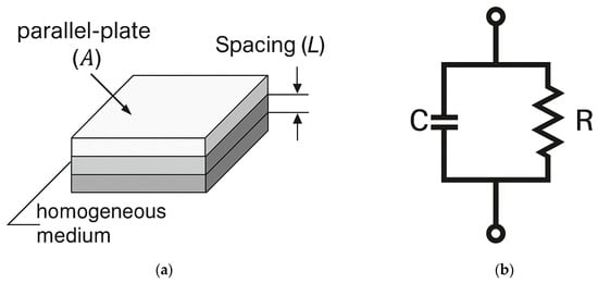
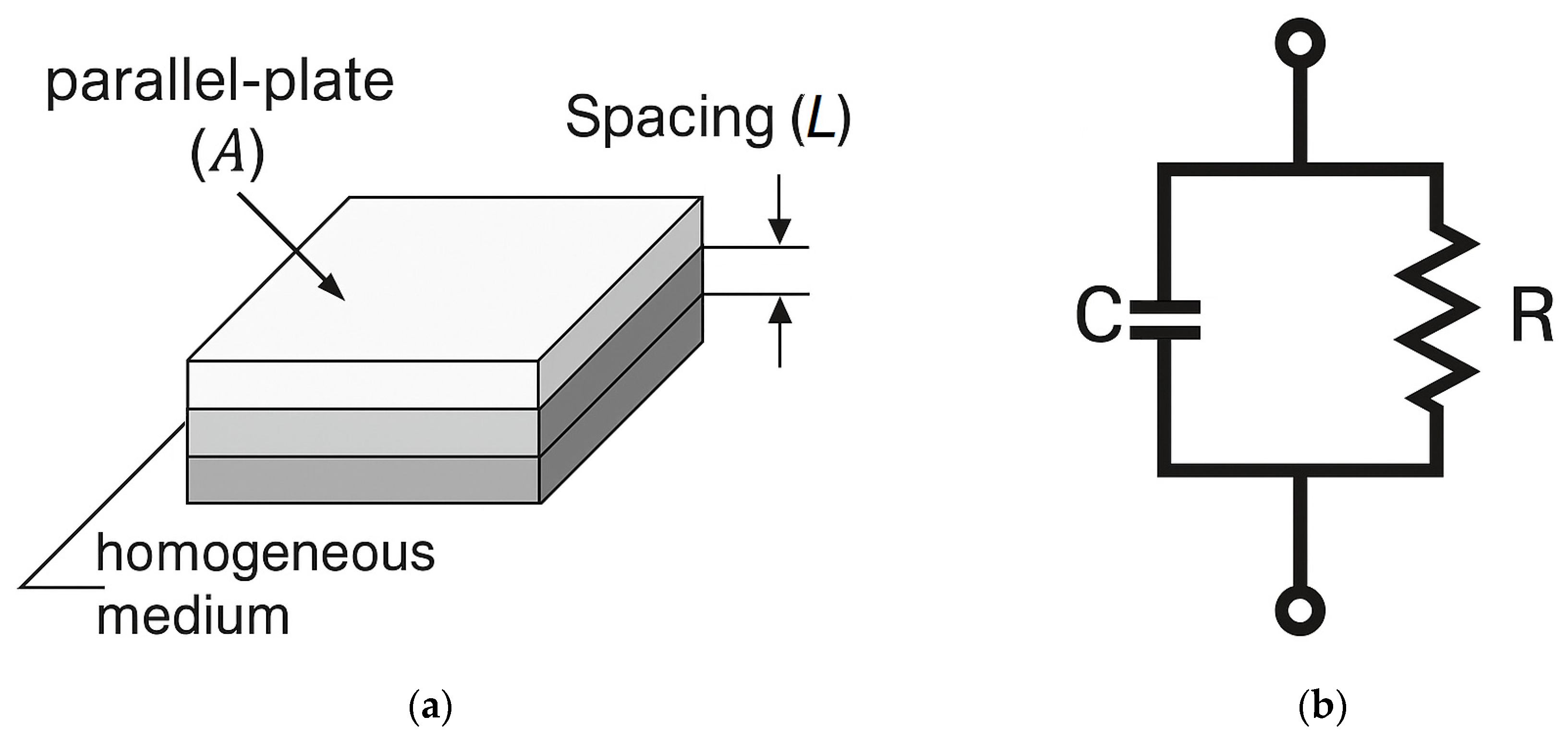
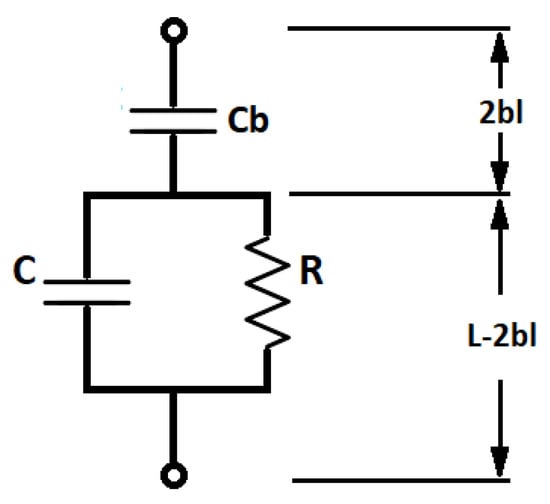
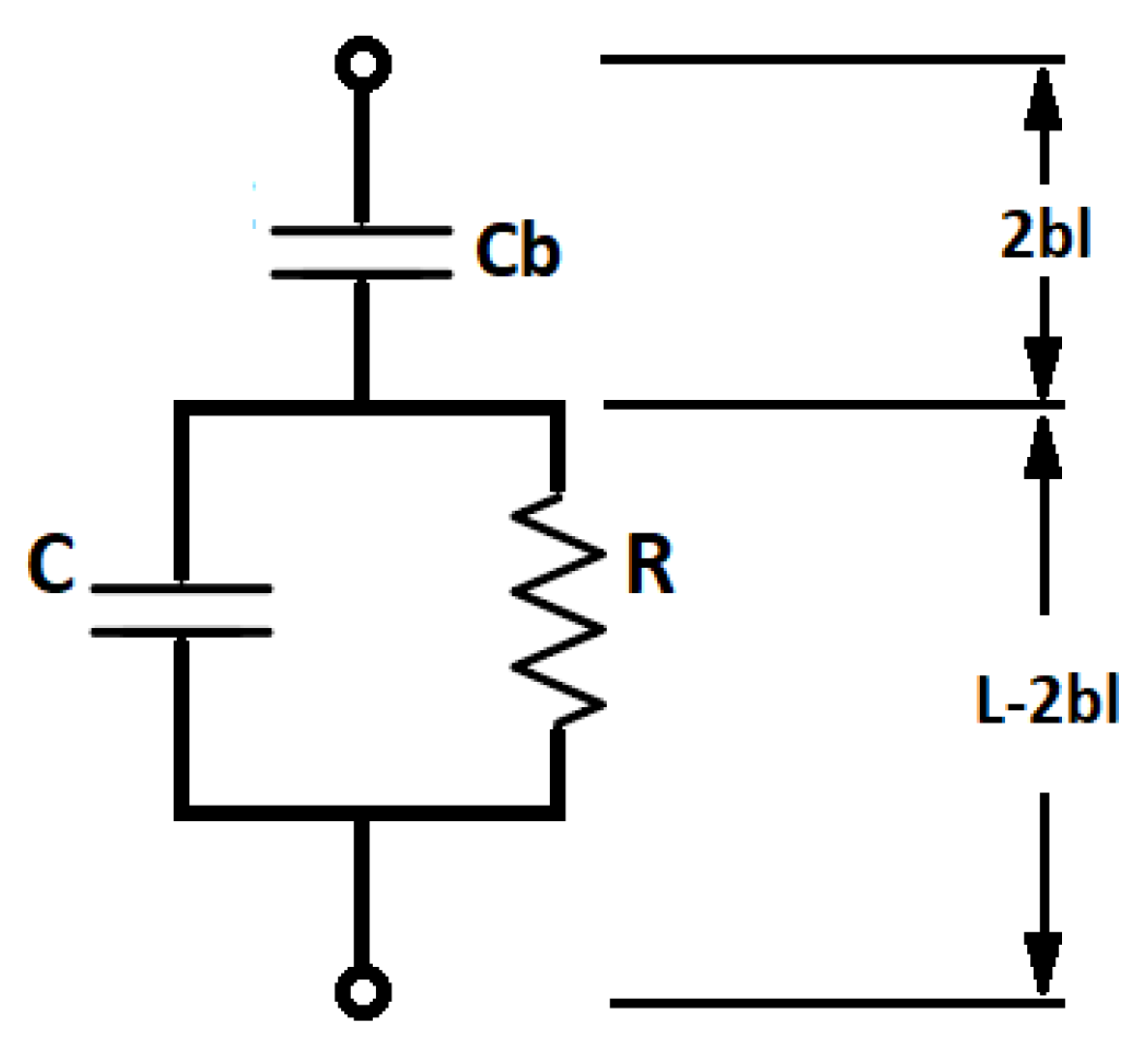
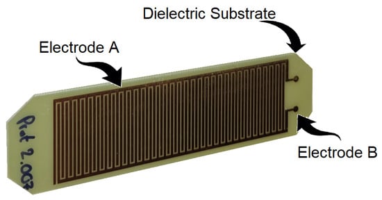
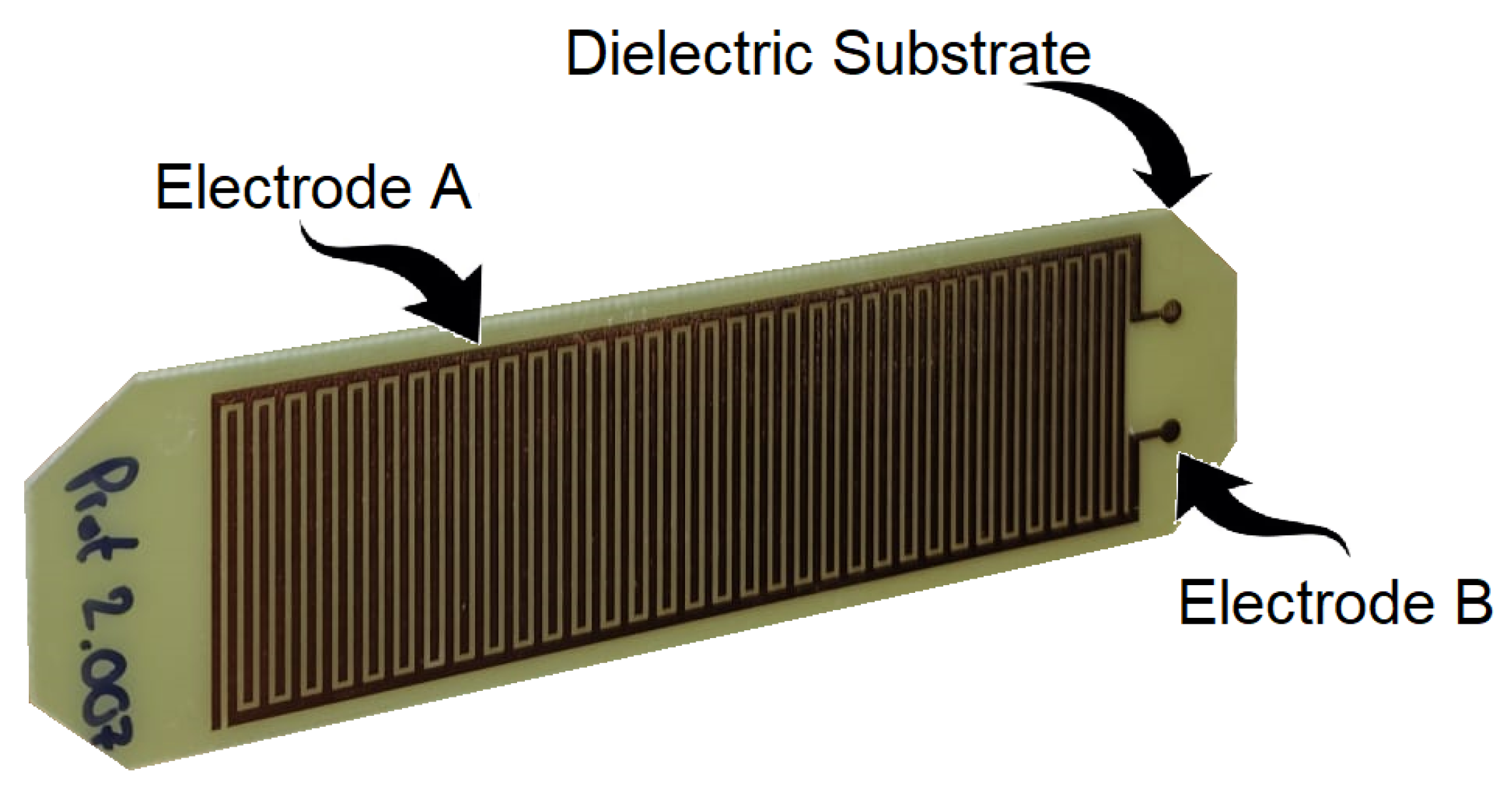
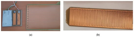
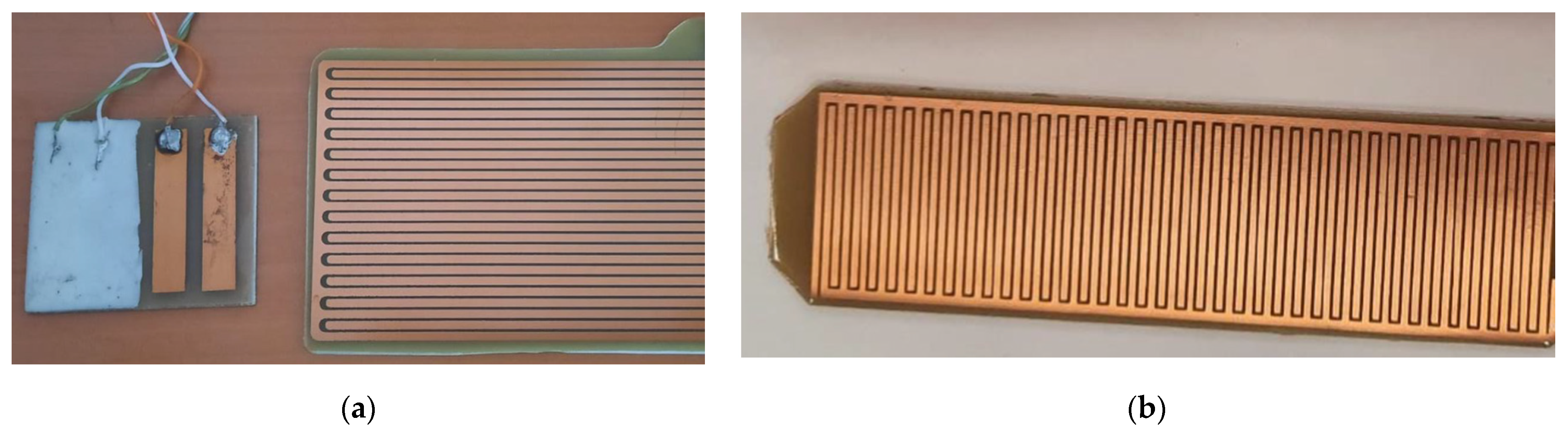
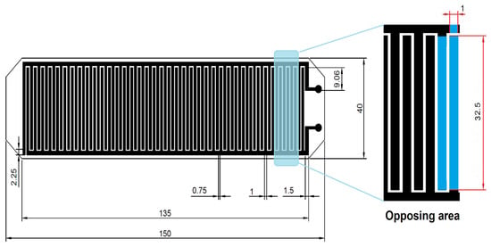
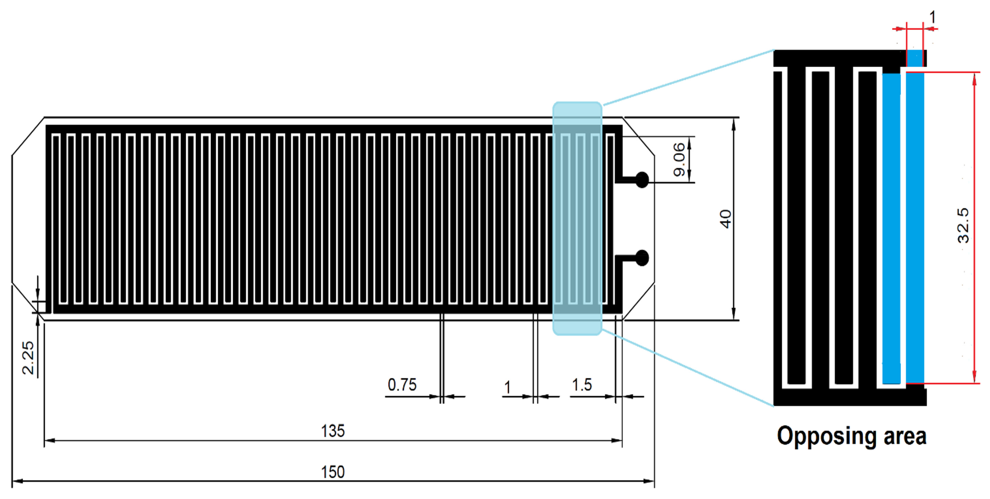
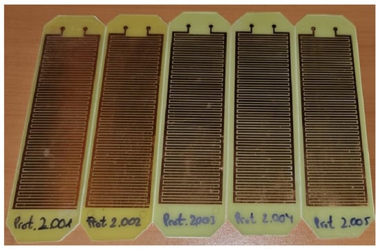
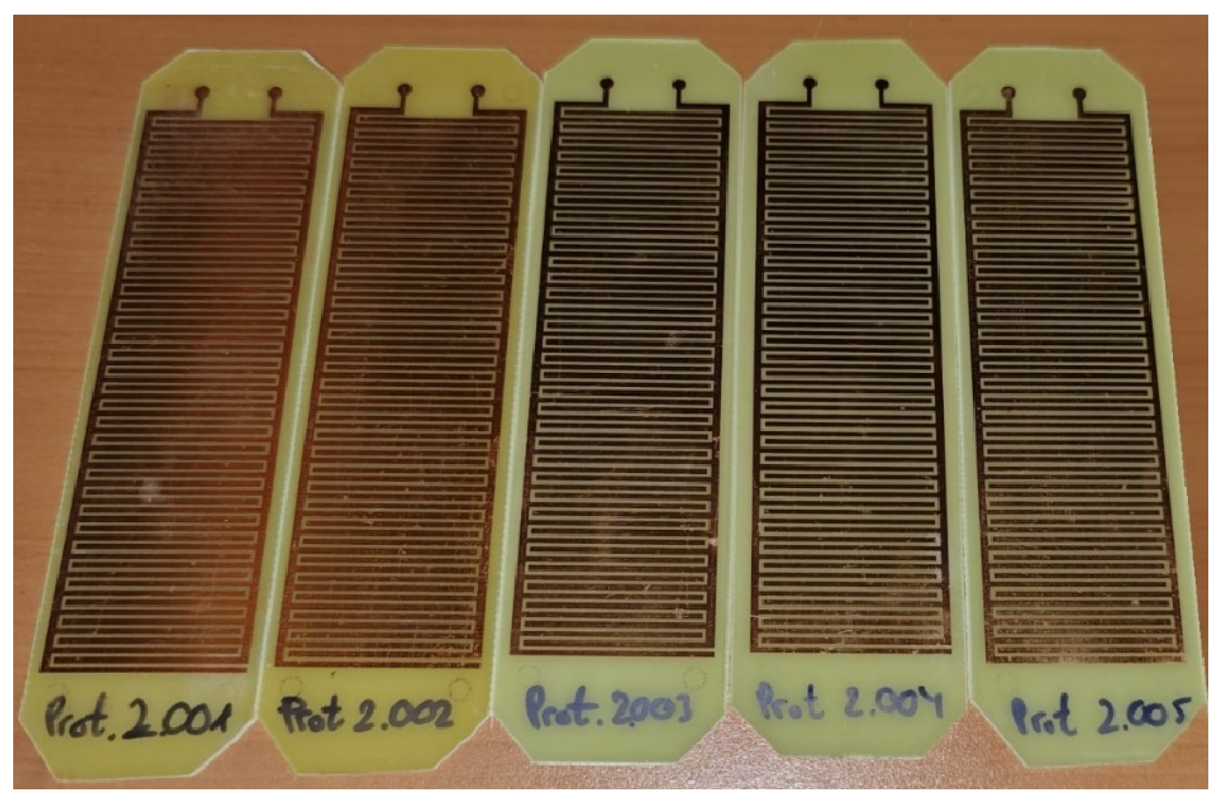
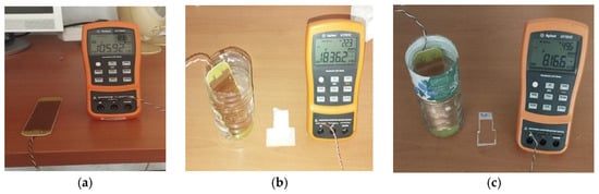
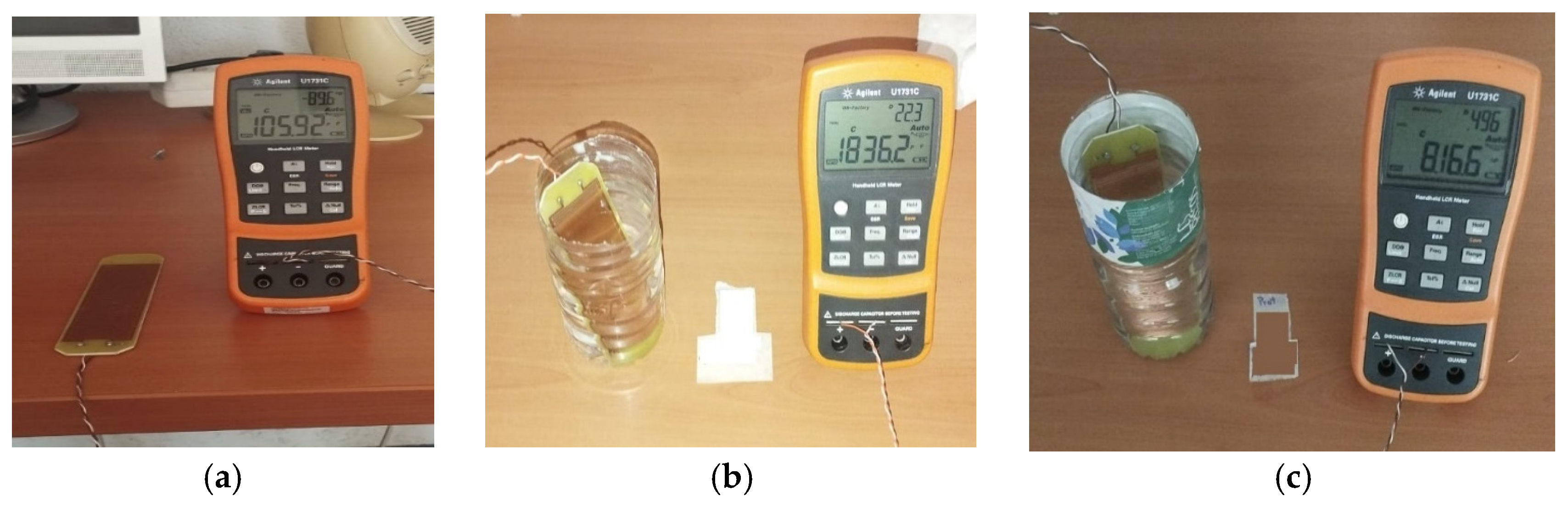
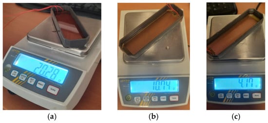
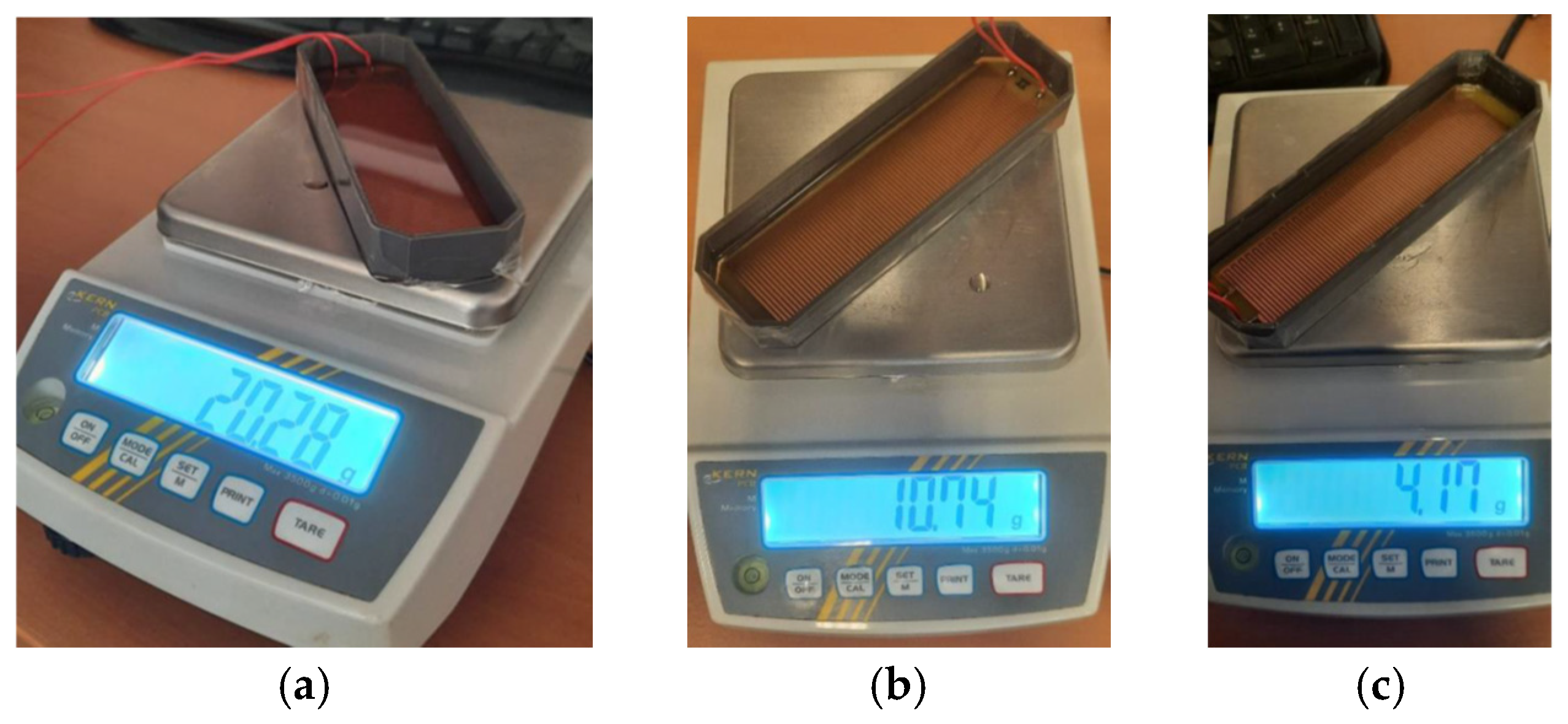
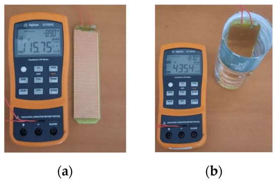
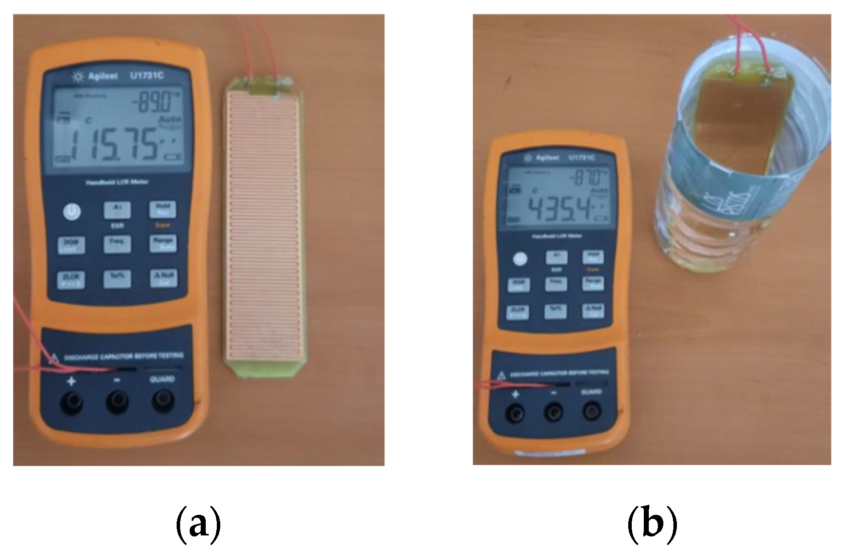
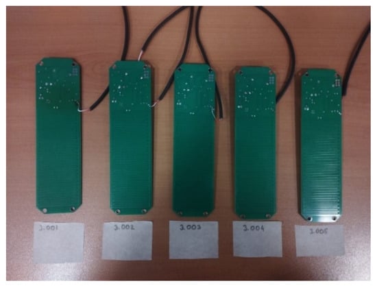
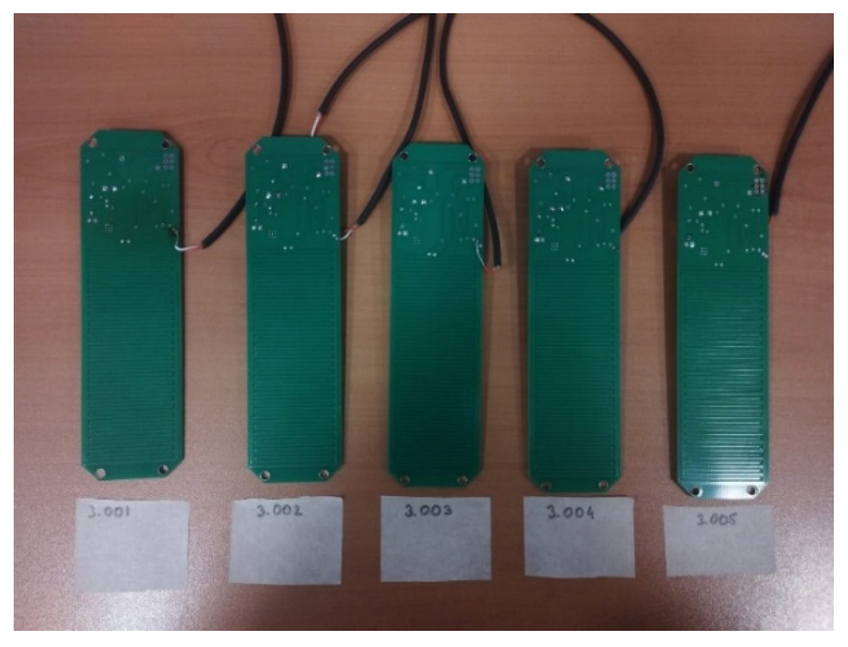
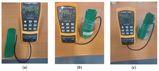
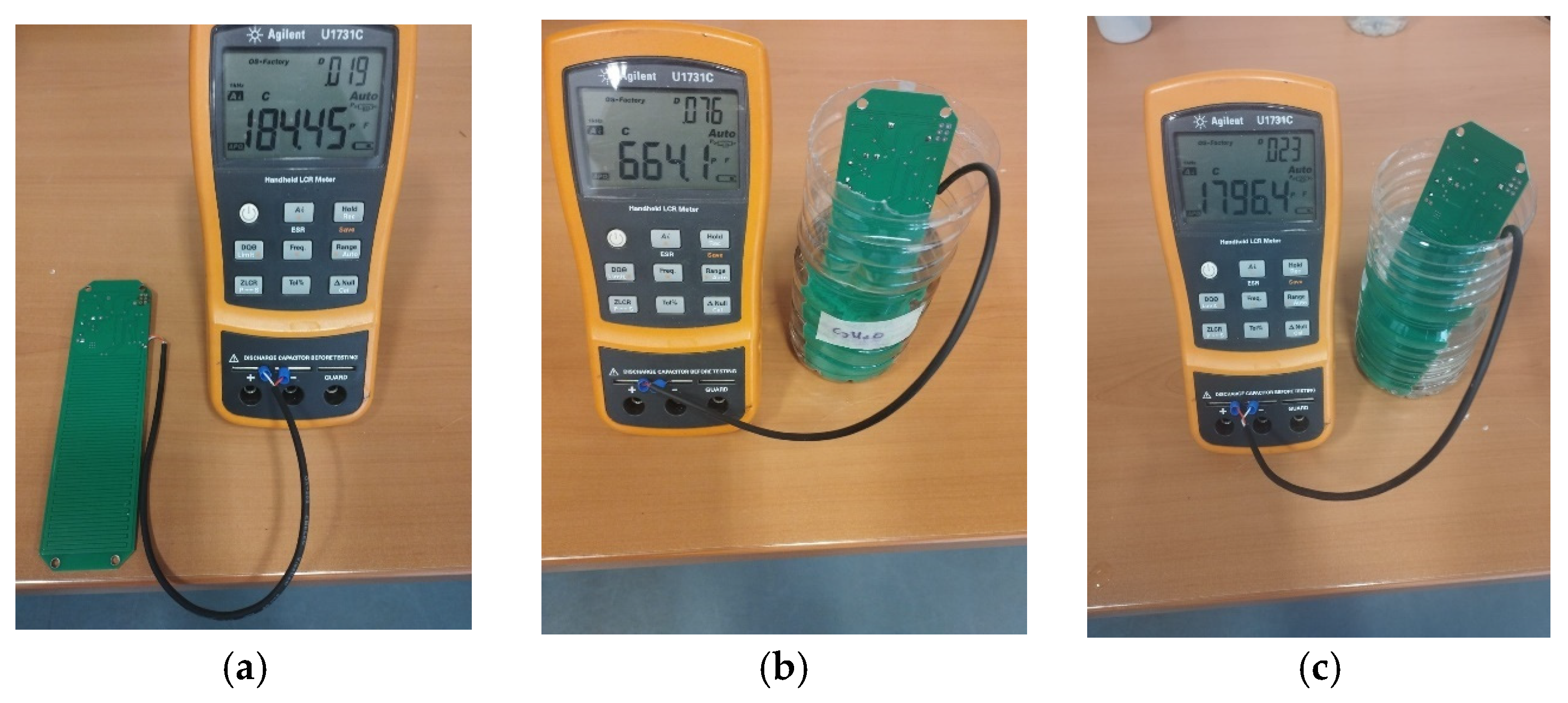
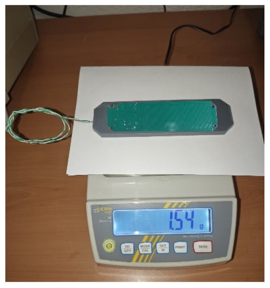
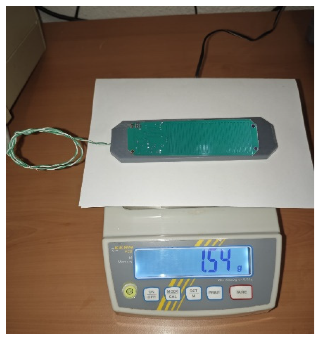
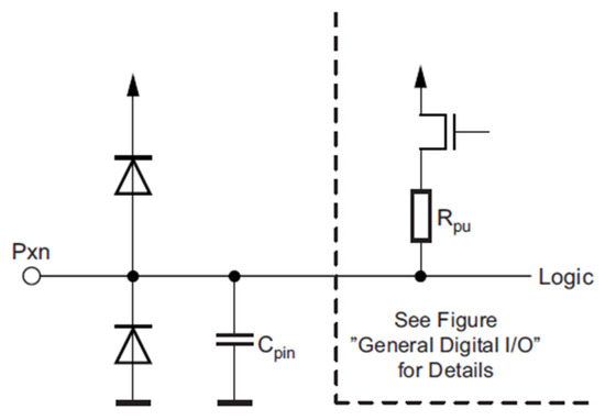
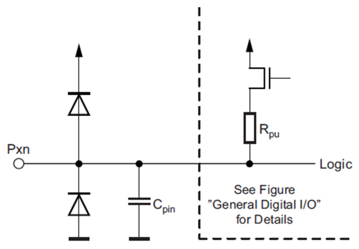
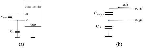
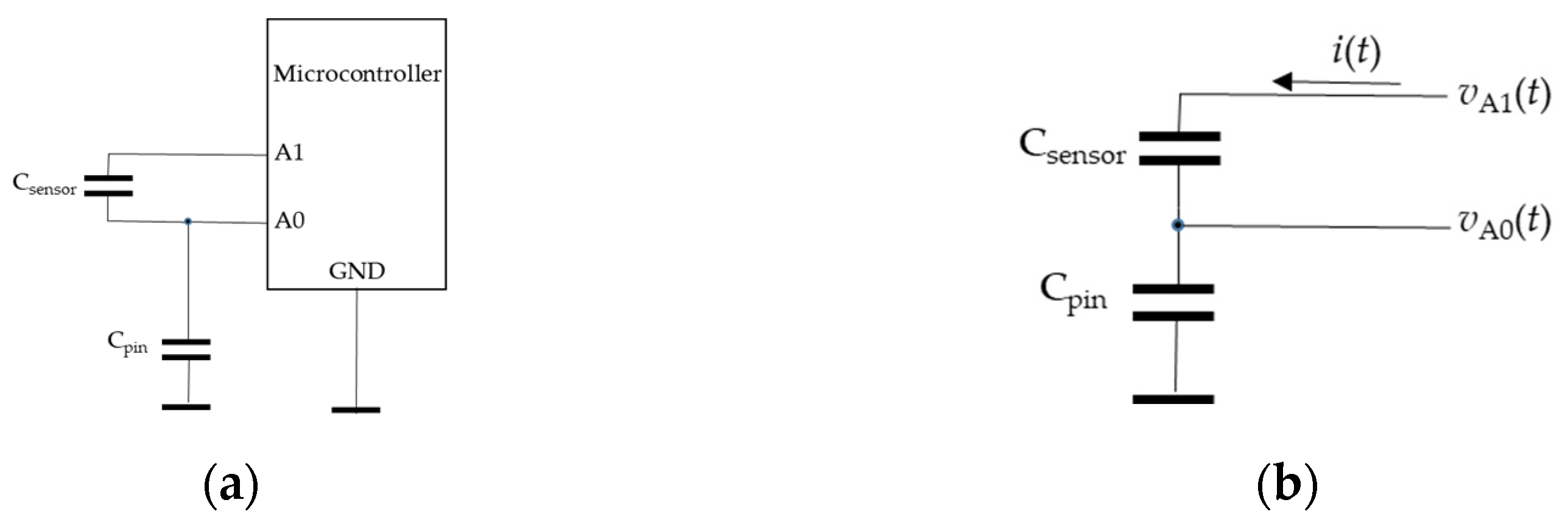
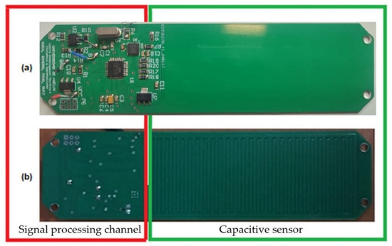
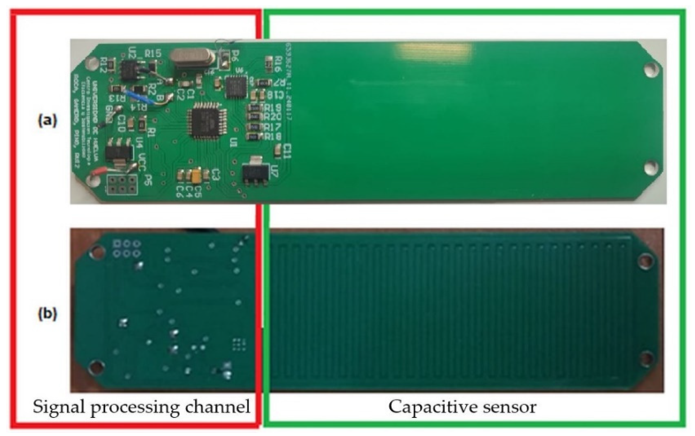
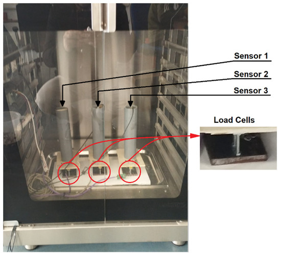
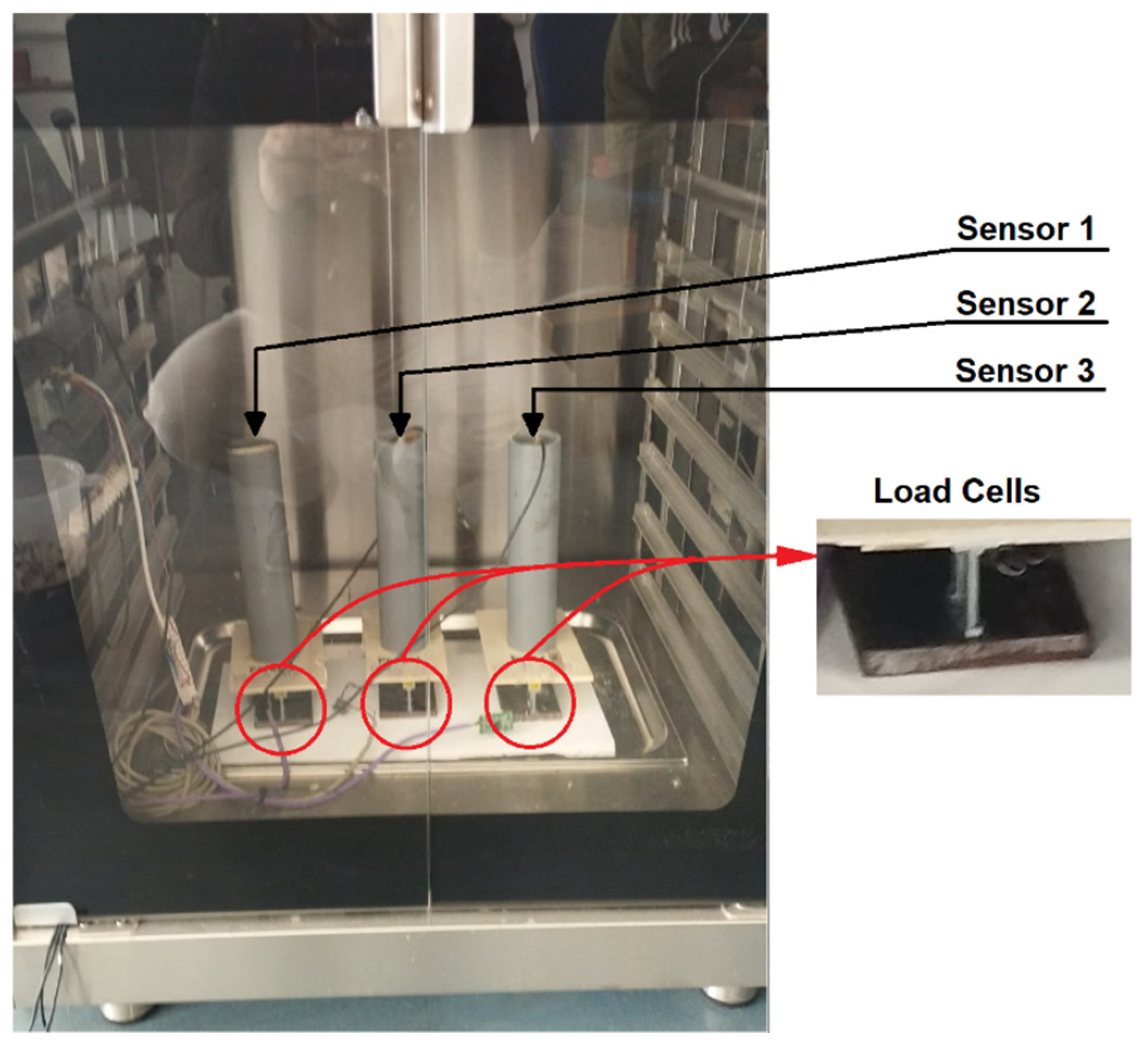
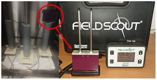
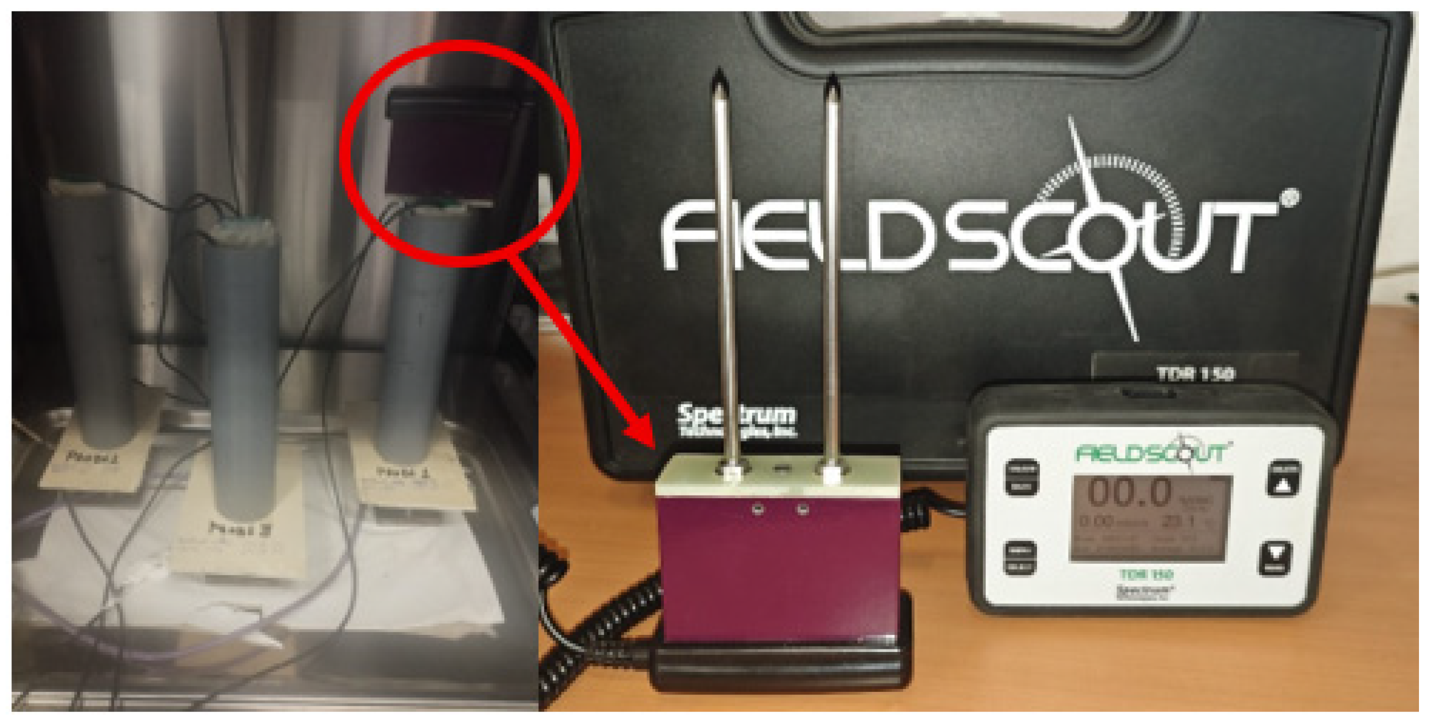
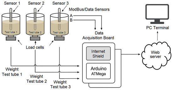
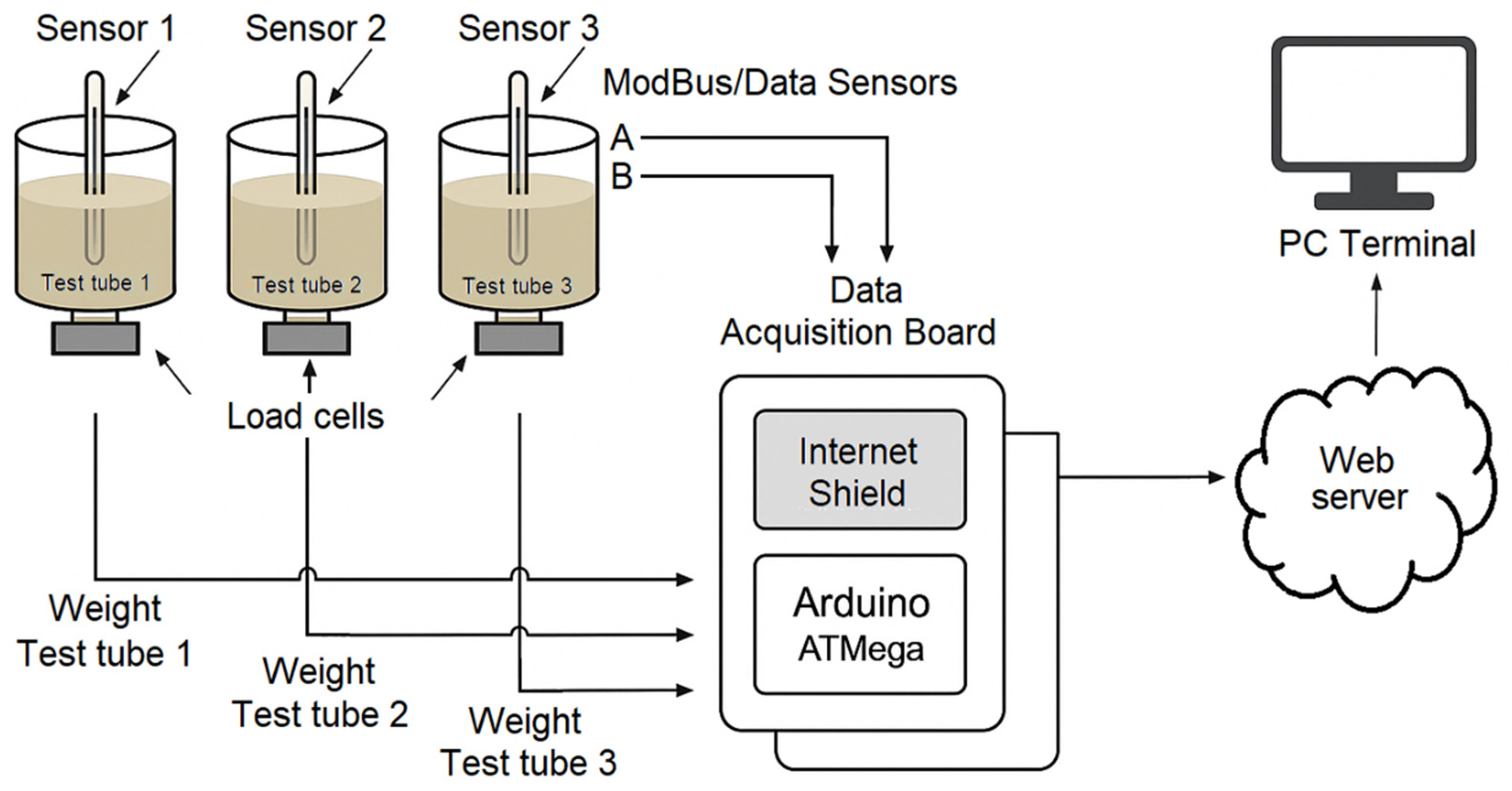
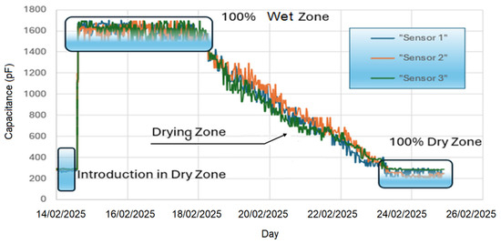
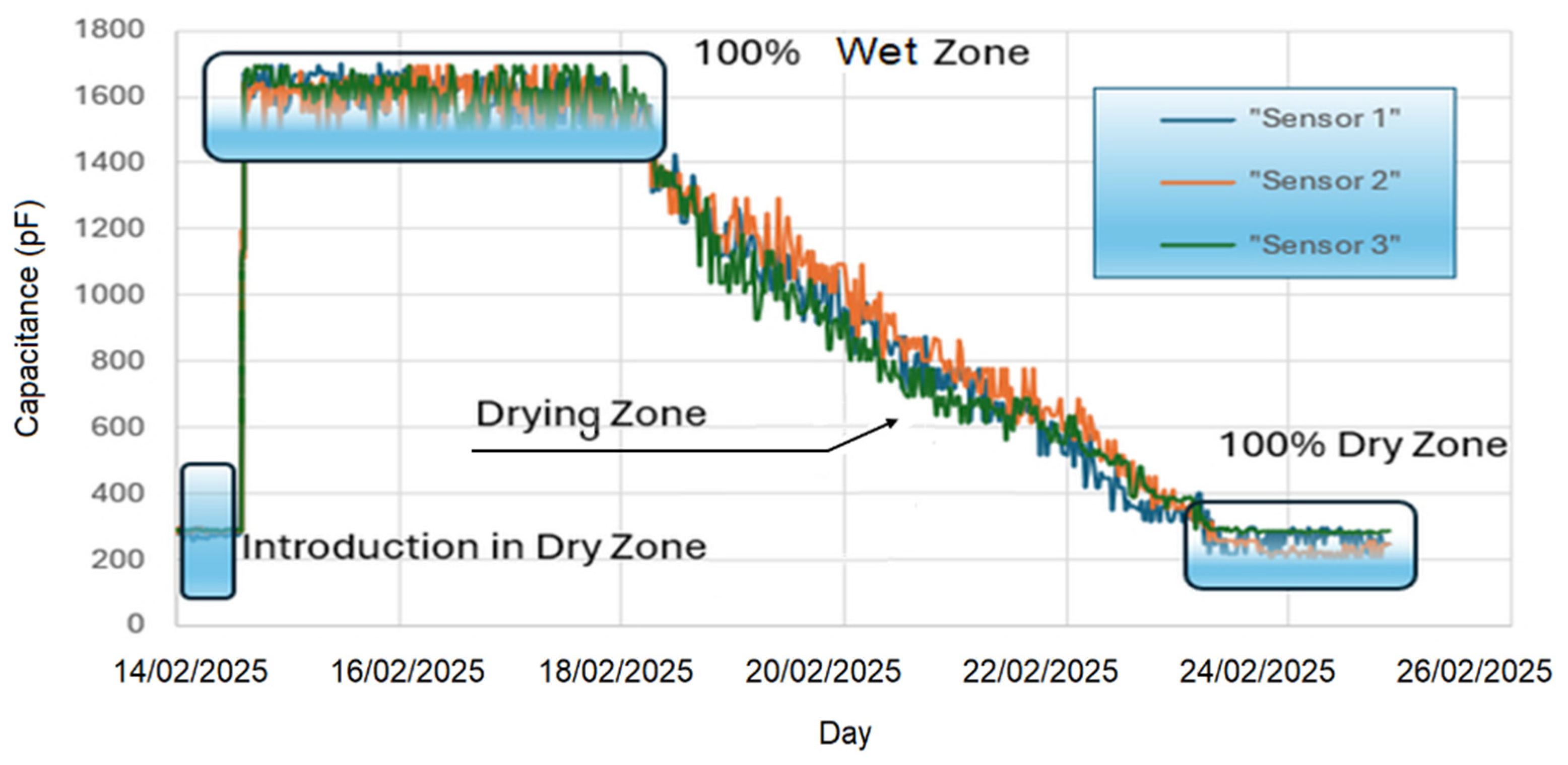
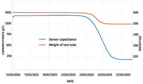
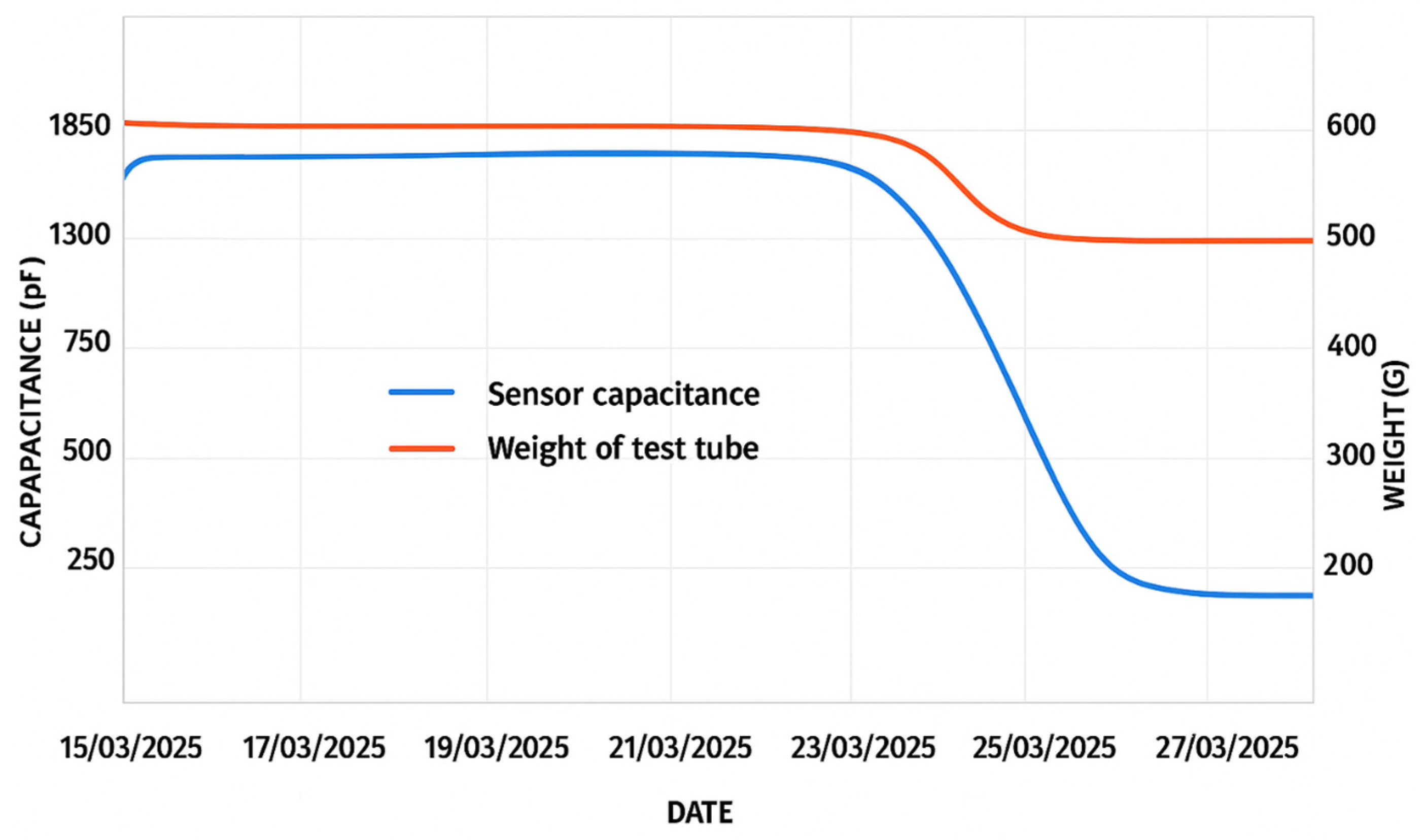
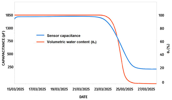
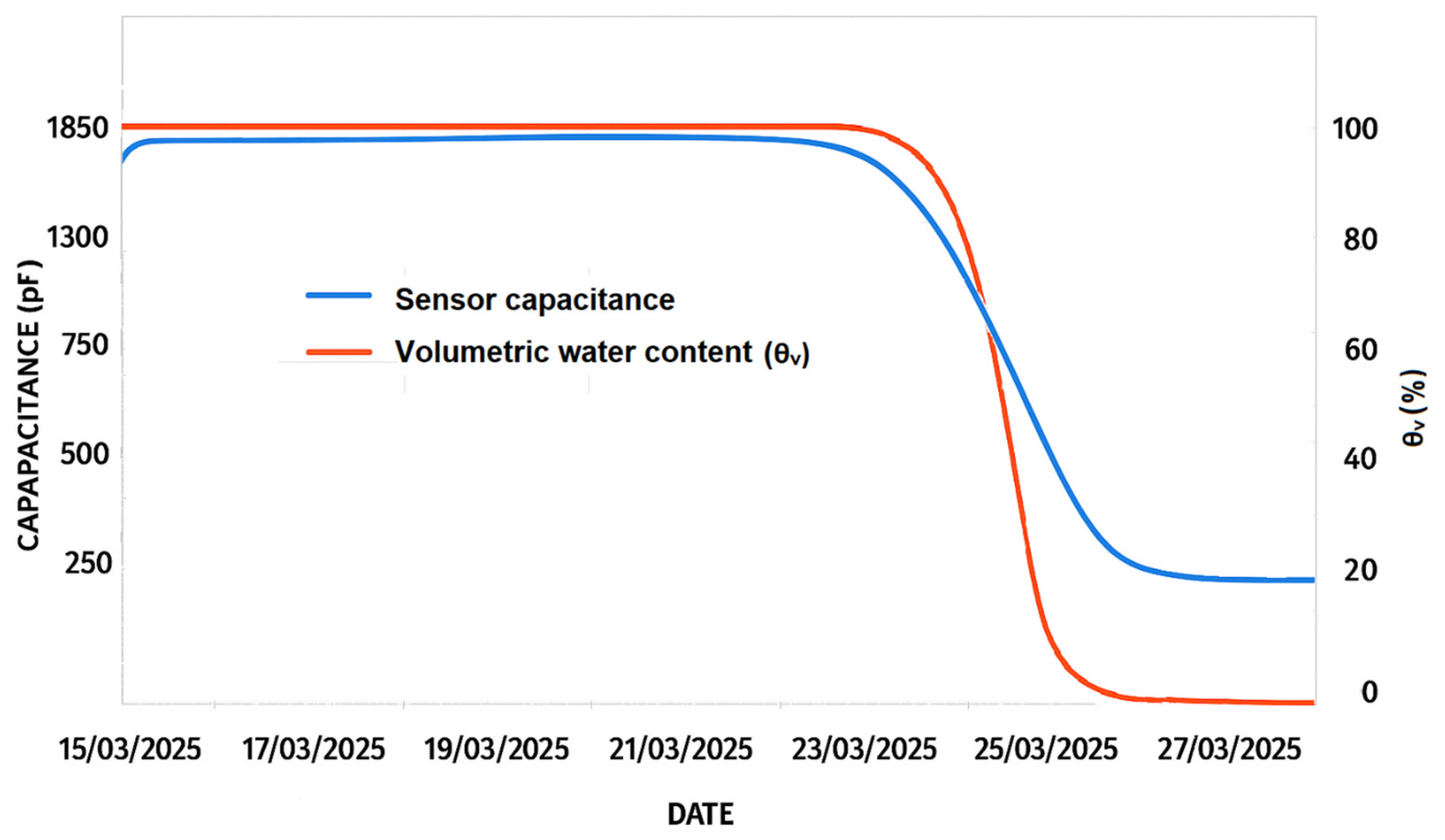
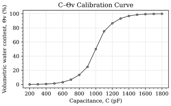
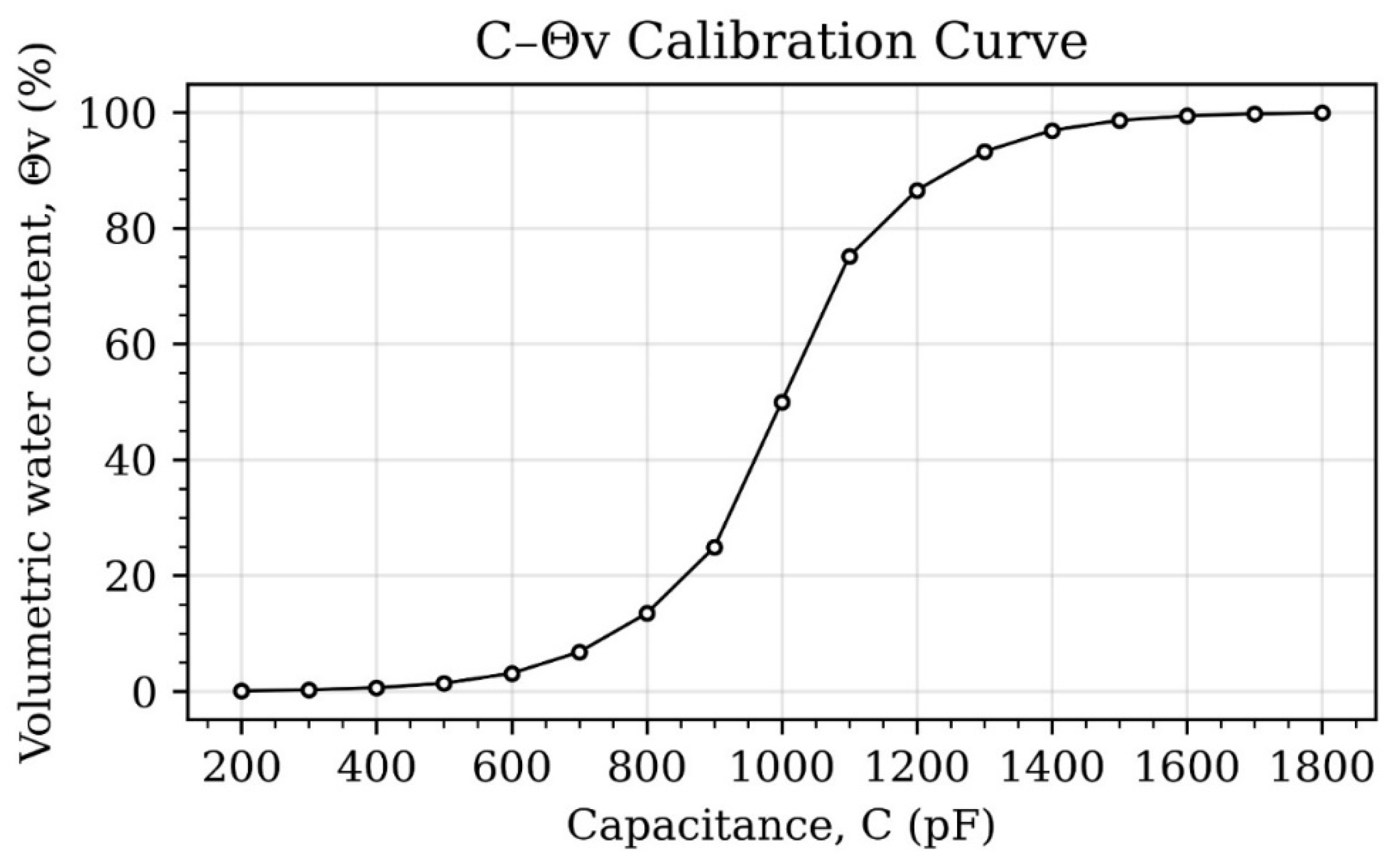
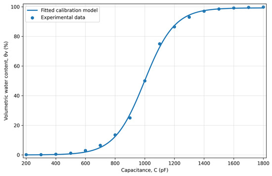
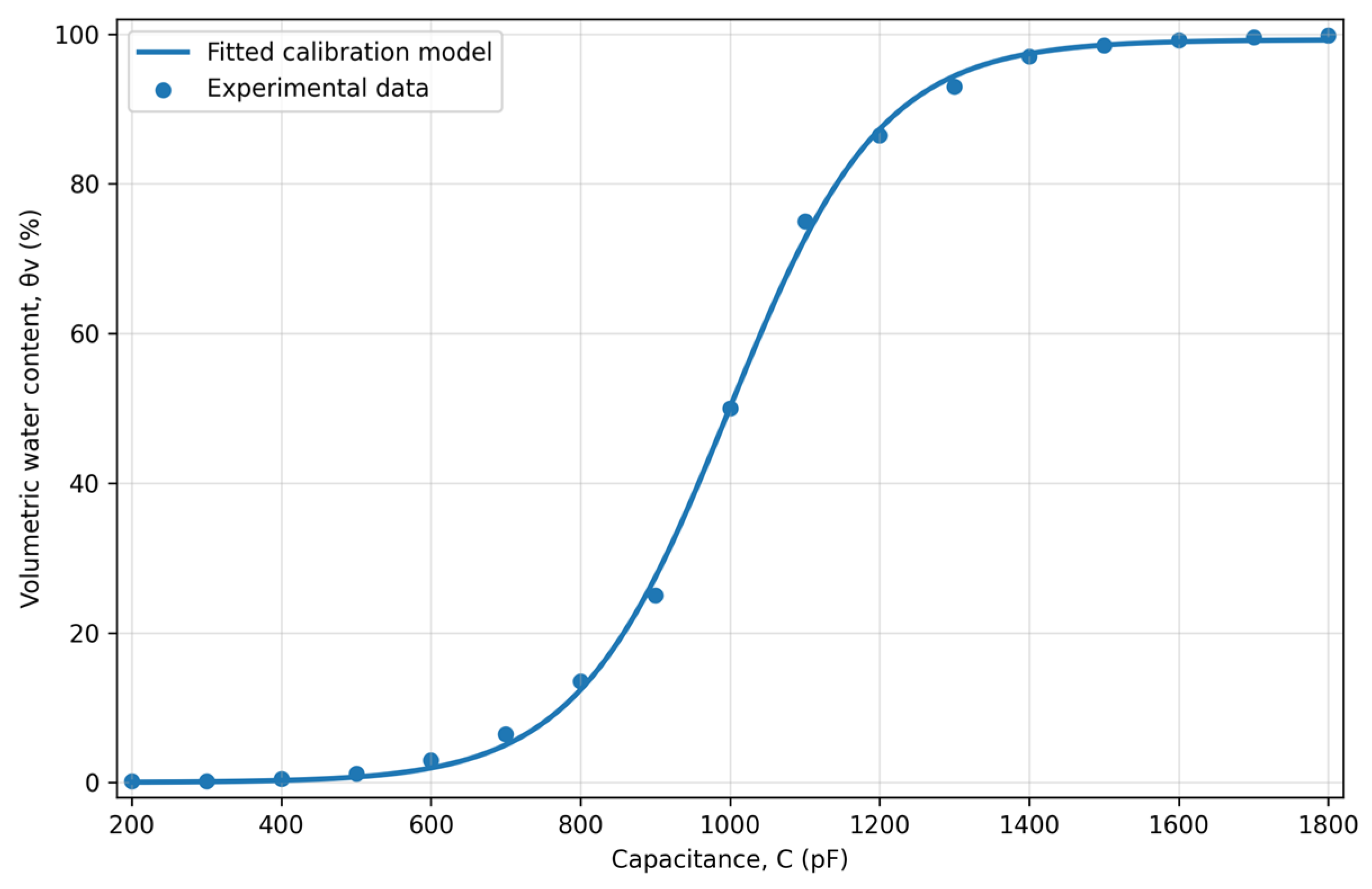

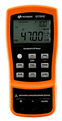
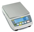
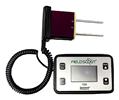
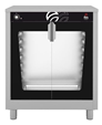
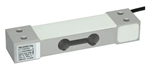
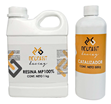
Disclaimer/Publisher’s Note: The statements, opinions and data contained in all publications are solely those of the individual author(s) and contributor(s) and not of MDPI and/or the editor(s). MDPI and/or the editor(s) disclaim responsibility for any injury to people or property resulting from any ideas, methods, instructions or products referred to in the content. |
© 2026 by the authors. Licensee MDPI, Basel, Switzerland. This article is an open access article distributed under the terms and conditions of the Creative Commons Attribution (CC BY) license.