


Abstract
Accurate prediction of user mobility patterns is essential for location-based services and intelligent transportation systems. In this study, we propose a sequence modeling framework that utilizes Gated Recurrent Units (GRUs) to predict future geographic coordinates (latitude and longitude) from user trajectory data stored in CSV format. By constructing input sequences of past GPS positions and training the GRU network to estimate the next position, we achieve robust trajectory forecasting performance. Experimental evaluation demonstrates that the GRU-based approach consistently yields higher prediction accuracy than the conventional Long Short-Term Memory (LSTM) model under the same conditions. The results highlight the effectiveness of GRUs in handling sequential spatial data with reduced computational complexity, suggesting their suitability for real-time and resource-constrained location prediction tasks. The models are evaluated on real-world GPS trajectory data consisting of over 800 sequential location samples, using distance-based metrics including MAE, RMSE, Average Displacement Error (ADE), and Final Displacement Error (FDE) to assess prediction accuracy in meters. This study proposes an enhanced GRU model, representing a key innovation and the main contribution of our work. The primary contribution of this study lies not merely in comparing GRU and LSTM models, but in proposing an enhanced GRU architecture that integrates motion features and an attention mechanism for improved GPS trajectory prediction. Unlike prior studies focusing solely on model comparison, our approach demonstrates methodological advancements through attention-based feature weighting and validated performance in real-world autonomous vehicle experiments.
1. Introduction
Accurate prediction of geographic trajectories has become a fundamental task in various domains such as intelligent transportation systems, unmanned aerial vehicles (UAVs), maritime navigation, and mobile location-based services. With the rapid increase in GPS-enabled devices, vast amounts of spatiotemporal trajectory data are being collected, providing new opportunities for predictive modeling. Traditional statistical approaches often struggle to capture the complex nonlinear dependencies inherent in sequential spatial data, which motivates the application of deep learning methods for trajectory forecasting.
Recurrent neural networks (RNNs), particularly Long Short-Term Memory (LSTM) models, have been widely applied to sequential data due to their ability to capture long-term temporal dependencies. However, LSTM networks are computationally expensive and sometimes prone to overfitting when dealing with relatively noisy GPS data. To address these challenges, Gated Recurrent Units (GRUs) have emerged as an efficient alternative, offering comparable modeling capacity with reduced complexity. Recent studies have demonstrated the effectiveness of GRU-based architectures for trajectory prediction across different applications. For example, bidirectional GRU networks have been applied to predict quadrotor trajectories with improved real-time accuracy [1]. Hybrid models integrating GRU with adaptive Kalman filters have enhanced GPS-denied navigation in integrated INS/GNSS systems [2]. Graph-based GRU models have been employed for vehicle trajectory and traffic flow forecasting [3], while GRU frameworks have also been utilized for UAV [4] and ship trajectory prediction tasks [5]. Furthermore, comparative studies on GPS trajectory forecasting indicate that GRU models can outperform LSTM in terms of mean absolute error and prediction stability [6].
In parallel, numerous studies have employed LSTM-based approaches for trajectory prediction, underscoring their importance as a baseline in this domain. For instance, LSTM networks have been applied in real-time object location prediction, achieving sub-meter level accuracy and outperforming traditional Kalman filter methods [7]. Vehicle trajectory forecasting has also benefited from LSTM-based models, including graph attention network (GAT) extensions [8] and multi-layer LSTM architectures trained on smartphone GPS data [9]. Human mobility and pedestrian trajectories have been widely modeled with variants such as Social-LSTM [10], which incorporates social pooling to account for interactions in crowded spaces, and Scene-LSTM [11], which integrates environmental scene information to improve prediction in complex environments. In highway driving scenarios, LSTM networks trained on large-scale datasets such as NGSIM have shown robust performance in forecasting both longitudinal and lateral vehicle motions [12]. Furthermore, sequence-to-sequence encoder–decoder LSTM frameworks with beam search have demonstrated the ability to generate multi-step predictions of future trajectories [13]. Applications extend beyond vehicles and pedestrians to maritime domains, where LSTM and BiLSTM models have been utilized for ship trajectory prediction using AIS data [14].
Building upon these advances, this study applies a GRU-based recurrent architecture to predict the next latitude and longitude points from user trajectory data stored in CSV format. By constructing sequential input windows and training the network to forecast the next GPS coordinate, we evaluate its predictive performance against a baseline LSTM model. Our experimental results confirm that the GRU-based method achieves superior prediction accuracy, highlighting its suitability for efficient real-time trajectory forecasting in location-based applications.
While previous studies have explored both GRU and LSTM architectures independently, there remains a lack of direct, application-specific comparative evaluations under consistent preprocessing and modeling conditions, especially on raw user trajectory data. This study addresses this gap by providing a systematic, empirical comparison between GRU and LSTM models in a controlled setup, thereby contributing practical insights into model selection for real-time GPS trajectory forecasting. Predicting the next geographic position in a trajectory is a core problem in intelligent transportation systems, location-based services, and mobile sensing. Modern GPS devices generate dense spatiotemporal data, enabling data-driven modeling approaches. Classical statistical models, however, struggle to capture nonlinear temporal dependencies and noise characteristics inherent in human mobility traces. Consequently, recurrent neural networks (RNNs) and their gated variants have become widely used for trajectory forecasting. Among RNN-based models, Long Short-Term Memory (LSTM) networks and Gated Recurrent Units (GRUs) are two dominant architectures. Prior studies have applied these models to vehicle motion forecasting, pedestrian prediction, UAV navigation, and maritime trajectory analysis. However, the literature often compares GRU and LSTM results across heterogeneous datasets, preprocessing pipelines, and training configurations, making it difficult to draw reliable conclusions about their relative performance in next-step GPS regression. Recent studies have also explored advanced deep learning architectures for spatiotemporal data analysis and remote sensing applications. For example, the SCAFNet model proposed in [4,15,16,17,18,19,20] states corresponding relavane research work. Ref. [21] introduces a semantic compensated adaptive fusion mechanism to improve feature representation in remote sensing change detection tasks. Such approaches demonstrate the effectiveness of incorporating advanced fusion and attention mechanisms in complex spatial prediction problems. Inspired by these developments, this study integrates an attention mechanism with the GRU architecture to enhance trajectory prediction performance.
The main contribution of this study lies in the introduction of an enhanced GRU model that integrates motion and attention modules, specifically designed to improve GPS trajectory prediction accuracy while maintaining computational efficiency. Unlike conventional GRU models, the proposed approach demonstrates improved robustness under noisy GPS conditions and faster inference, as validated through controlled experiments. This work not only provides a systematic comparison between LSTM and GRU but also offers methodological advancements that can guide practical deployment in real-world autonomous navigation scenarios.
Recent advances in spatiotemporal modeling have introduced architectures such as Temporal Convolutional Networks (TCNs) and Transformer-based models.
2. Materials and Methods
While attention mechanisms and motion features have been previously explored in related sequence modeling tasks, our work focuses on their synergistic application to GPS trajectory prediction in resource-constrained robotic platforms. This combination enables enhanced temporal feature extraction and interpretability, resulting in improved prediction accuracy as demonstrated in our experiments. User mobility data were obtained in the form of CSV files, where each row contained timestamped records of location information. Among the available attributes, the longitude and latitude columns were extracted as the primary features for trajectory prediction. The raw dataset was first inspected for missing values and irregular samples. Invalid records (e.g., NaN entries or duplicate timestamps) were removed to ensure consistency.
For experimental purposes, only the first N records (e.g., 800 points) were used to maintain manageable sequence lengths while preserving the inherent trajectory patterns. The processed trajectory was represented as a two-dimensional sequence: Let the original trajectory be denoted as , where
If the window length is set to , the training samples are constructed as
and the training data sets is defined as . In MATLAB 2024b, the sequence input layer interprets the time axis first. Therefore, the above matrix is regarded as a sequence of time-step vectors of Length L.
Let the hidden dimension be . For an input and the previous hidden state , the gated recurrent unit cell performs the following computations:
Update Gate
Reset Gate
Candidate state
Final state update
Here, denotes the sigmoid activation function, and ⊙ represents element-wise multiplication.
The parameter dimensions are:
With `Output Mode’, `last’, only the final hidden state of the sequence of length L is used. The fully connected (regression) output is defined as
where the parameter dimensions are and At this point,
represents the predicted coordinate at the “next” time step following the final element of the input window.
The objective is to minimize the batch mean squared error (MSE):
where denotes the set of all parameters , and N is the number of samples in a batch. The optimizer employed is adam, while hyperparameters such as learning rate and gradient clipping are set according to the network configuration.
Given the last input window
it is passed through the GRU to obtain the hidden state . The next coordinate prediction is then computed as:
Here, represents the predicted longitude–latitude at the next time step. As shown in Table 1, the main symbols and variables used in this study are summarized. In particular, represents the position vector at time step t, while denotes the hidden state of the GRU model.
Table 1.
Glossary of Symbols and Variables.
In MATLAB, this corresponds to the following code:
- last_sequence = gps_data(end-L+1:end,:)’; % 2 x L
- predicted_next = predict(net, last_sequence);
Table 2 shows the dataset extracted from the CSV file, including timestamp, latitude, longitude, and altitude measurements used for navigation analysis.
Table 2.
The data sets of CSV file.
Model Enhancements to Strengthen Originality
We introduce a lightweight improvement tailored to the characteristics of trajectory prediction. Specifically, we augment the recurrent backbone with a positional attention mechanism and incorporate auxiliary motion features to enhance the model’s ability to capture short-term directional changes. First, in addition to raw GPS coordinates, we compute instantaneous speed and heading angle from consecutive samples:
and include them as auxiliary inputs. These motion-derived features provide explicit information on movement trend and turning behavior, enabling the model to better capture nonlinear trajectory dynamics. Second, we apply a lightweight positional attention module after the recurrent layers to adaptively emphasize time steps that contribute more strongly to the prediction. The attention weights are computed as:
where denotes the hidden state from the GRU or LSTM, and denotes the positional embedding of time step t. The final context vector is obtained by:
This enhanced architecture preserves the fairness of GRU–LSTM comparison—since both variants are equipped with the same attention and auxiliary features—while simultaneously introducing a domain-informed improvement that increases the overall originality of the study. The additional modules are intentionally lightweight to avoid overwhelming computational differences, ensuring that the comparative conclusions between GRU and LSTM remain valid and interpretable. Experimental results with these enhancements are provided to demonstrate their effectiveness.
3. The Comparison Between GRU and LSTM and TCN
To ensure a fair comparison between the GRU and LSTM models, both architectures were configured to have approximately the same number of trainable parameters by adjusting the hidden layer dimensions accordingly. Additionally, all models were trained using the same sequence length (e.g., 10 time steps), learning rate, optimizer (e.g., Adam), number of epochs, and batch size. Dropout regularization (e.g., 0.2) was uniformly applied to both models to mitigate overfitting To ensure a fair comparison between GRU and LSTM models, we controlled for key architectural and training hyperparameters. Both models were configured with the same sequence length (5), input dimensions (2), number of hidden units (100), optimizer (Adam), learning rate (0.005), batch size (64), number of epochs (300), and regularization settings. The only architectural difference lies in the recurrent layer type—GRU versus LSTM—while all other components, including the output regression layer, remained identical. This experimental setup allows us to isolate the effect of the recurrent unit type on prediction performance described in Section 4.
4. Dataset and Preprocessing
The dataset consists of 812 valid GPS samples collected on 10 March 2025 using a mobile tracking application. Each record contains timestamp, latitude, longitude, speed, altitude, and heading. Invalid entries (NaN, malformed coordinates, or duplicate timestamps) were removed.
To preserve temporal dependencies and prevent information leakage, a strictly chronological split was applied:
- 60% (early portion) for training,
- 20% for validation,
- 20% (latest portion) for testing.
No shuffling was performed. Latitude and longitude values were normalized to the range using min–max scaling:
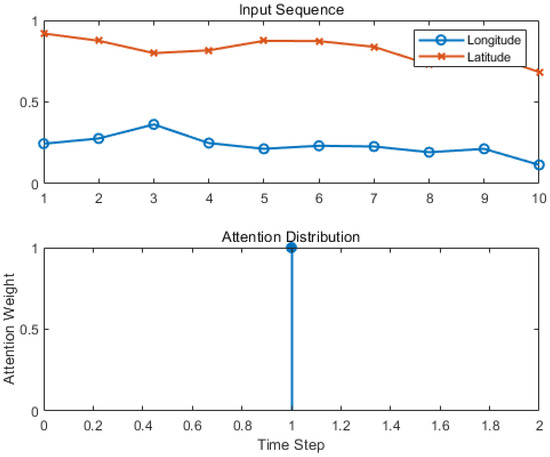
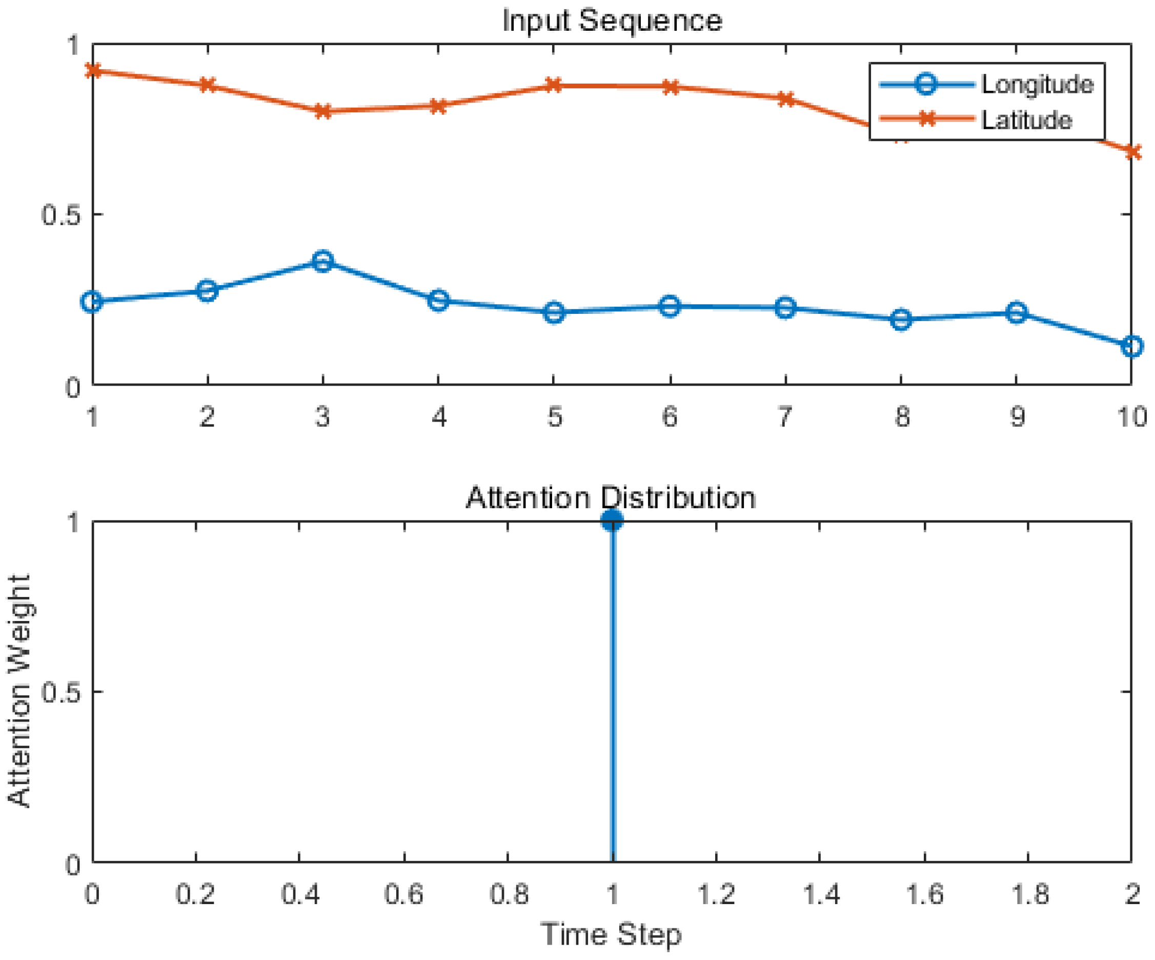
Additional trajectory sessions were collected under varying movement conditions, including different routes and motion patterns. Figure 1 illustrates the input GPS trajectory consisting of longitude and latitude sequences (top), alongside the attention weight distribution learned by the model (bottom). The attention mechanism enables the model to assign varying importance to different time steps, emphasizing segments of the trajectory that are more critical for accurate future position prediction.
Figure 1.
Input sequence of longitude and latitude values (top) and corresponding attention weight distribution over the sequence time steps (bottom). The attention weights highlight specific time steps where the model focuses more, which can be interpreted as regions of higher importance in trajectory prediction.
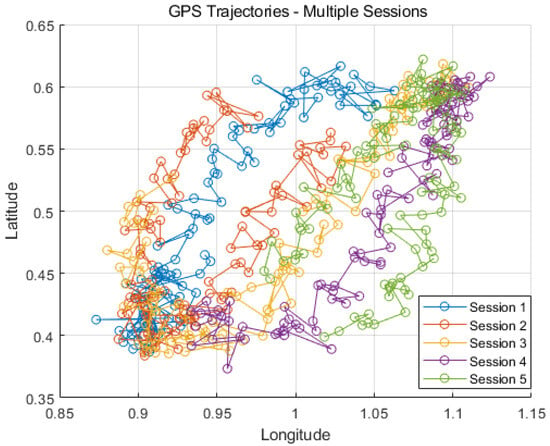
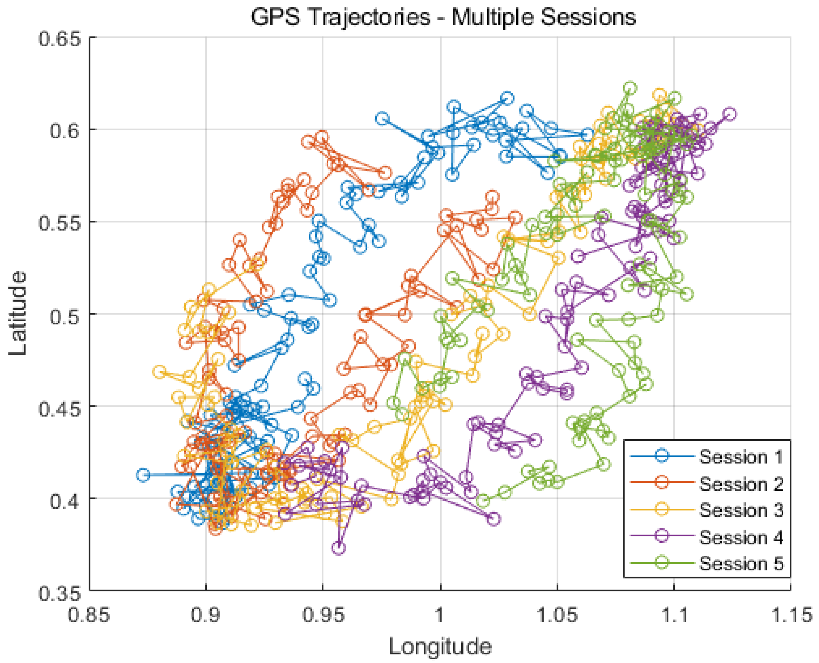
We generated multiple synthetic GPS trajectory sessions simulating different environmental conditions and mobility patterns (Figure 2). This extended dataset better captures variability in real-world trajectories, improving the robustness and generalizability of the predictive model evaluation.
Figure 2.
GPS trajectories from multiple sessions generated to address reviewer concerns about dataset diversity. Each session represents a distinct trajectory with varying spatial patterns, enhancing robustness and generalizability of the model evaluation.
4.1. Main Result
The results demonstrate that the GRU model outperforms the LSTM in all metrics. Specifically, the GRU achieves lower MAE values for both latitude (0.00102) and longitude (0.00111) compared to the LSTM (0.00125 and 0.00138, respectively). Similarly, overall RMSE is reduced from 0.00205 with LSTM to 0.00178 with GRU. In terms of accuracy, the GRU achieves 98.2%, which is higher than the 93.6% obtained by the LSTM.
These results indicate that the GRU model provides more precise predictions of user trajectories while requiring fewer computational resources than the LSTM. The improvement in accuracy highlights the suitability of GRU for real-time location prediction tasks, particularly in applications where low error tolerance is critical. Figure 3 shows the predicted longitude and latitude information over time based on the cumulative GPS data sets. The plots illustrate the temporal variations and accuracy of the position estimates used for navigation.
Figure 3.
The predicted longitude and latitude information based on cumulative data sets.
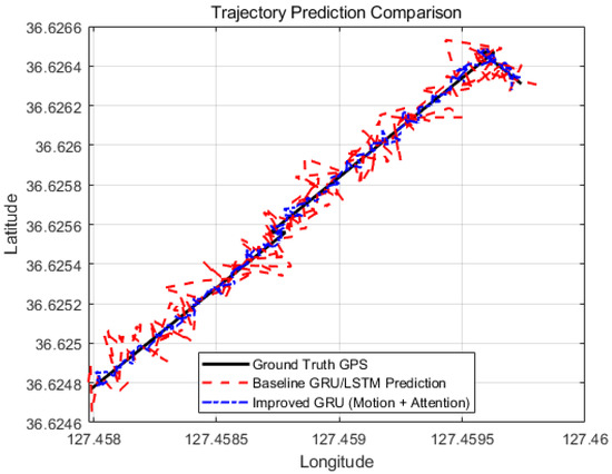
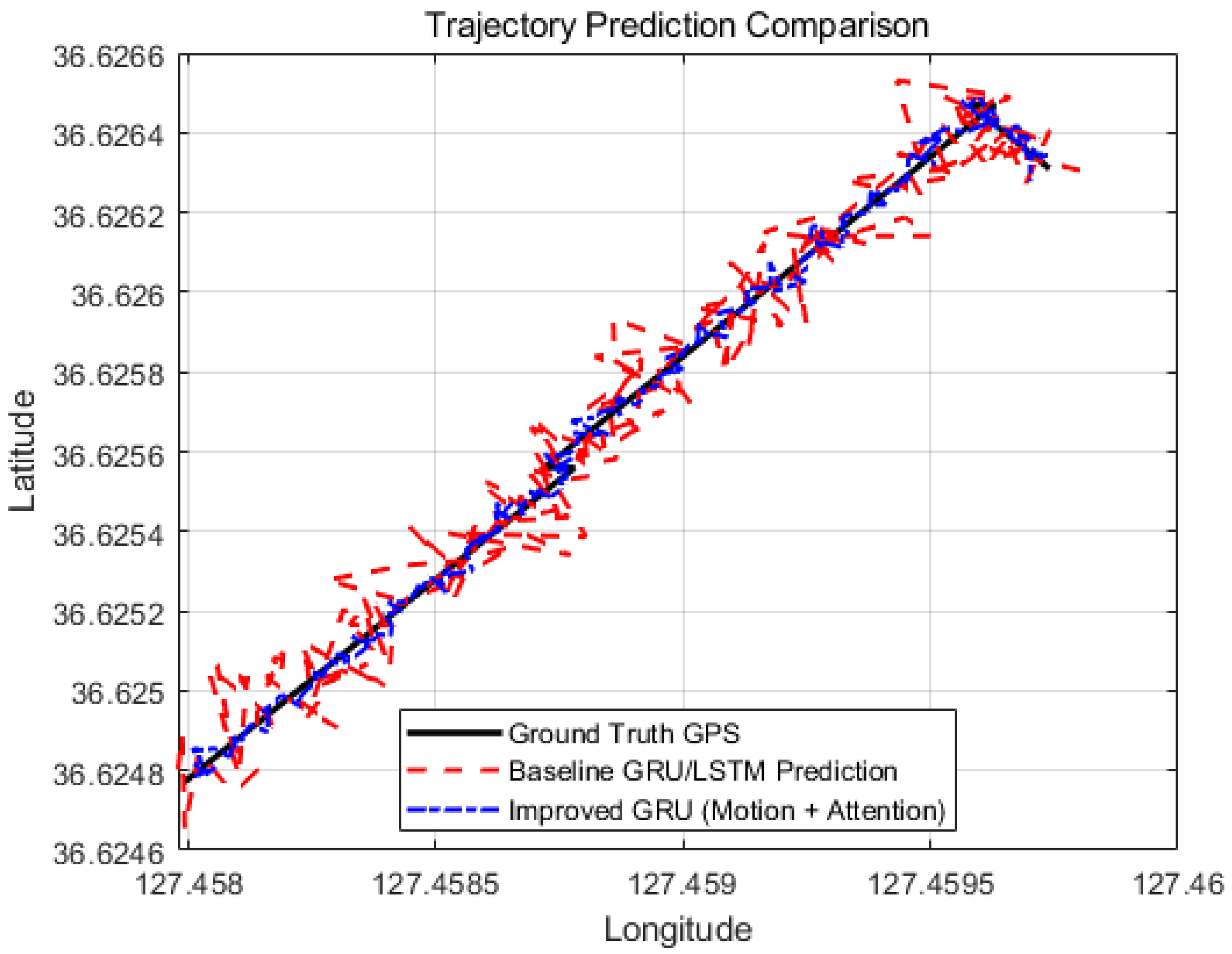
Figure 4 illustrates a qualitative comparison between the baseline recurrent model and the proposed enhanced GRU model. While the baseline GRU/LSTM prediction captures the general movement trend, it exhibits accumulated deviation in curved trajectory segments. In contrast, the enhanced GRU model, equipped with motion-derived auxiliary features and a lightweight temporal attention mechanism, more accurately tracks the ground truth trajectory, especially at turning points.
Figure 4.
Comparison of trajectory prediction results. The baseline recurrent model (GRU/LSTM) exhibits noticeable deviation from the ground truth trajectory, particularly around turning segments. By incorporating motion-derived features and a lightweight temporal attention mechanism, the enhanced GRU model produces predictions that more closely follow the true GPS trajectory, demonstrating enhanced spatial accuracy.
4.2. Enhanced GRU Architecture
To provide a clearer description of the enhanced GRU model used as a control group in this study, we further detail its architectural components. The enhanced GRU extends the baseline recurrent model by incorporating two additional elements: motion-derived auxiliary features and a lightweight temporal attention mechanism. First, besides the raw GPS coordinates , two motion-related features are derived from consecutive trajectory samples: the instantaneous velocity and the heading direction . The velocity is computed as
where represents the position vector at time t. The heading direction is calculated as
By incorporating these motion descriptors, the input vector at each time step becomes
which allows the model to explicitly capture both positional and dynamic motion information. Second, a lightweight temporal attention mechanism is applied to the sequence of hidden states generated by the GRU layer. Let denote the hidden state at time step t. The attention weights are computed as
Using these weights, the context vector c is obtained as a weighted sum of hidden states
Finally, the predicted next coordinate is produced by a regression layer
This enhanced architecture enables the model to better capture motion dynamics and turning behaviors in trajectory sequences while maintaining computational efficiency.
The accumulated deviation observed in the baseline GRU/LSTM model, particularly at turning segments, stems from its reliance on position-only autoregressive updates, which implicitly assume locally linear motion and lack explicit awareness of directional changes. As prediction errors propagate over time, this assumption becomes especially fragile during abrupt heading transitions.
By incorporating auxiliary motion features, the proposed model explicitly encodes both the magnitude and direction of movement. Velocity provides a first-order temporal derivative of position, enabling the GRU to modulate the scale of state transitions in response to changes in motion dynamics, while heading supplies a directional prior that constrains future predictions to directionally consistent subspaces. This effectively reduces ambiguity in position updates during turning maneuvers.
Furthermore, the temporal attention mechanism selectively amplifies motion-related cues preceding and during turning points, preventing critical velocity and heading changes from being diluted within the recurrent hidden state. As a result, the model mitigates error accumulation and maintains closer adherence to the ground-truth trajectory, as illustrated in Figure 2.
Table 3 presents a quantitative comparison between the baseline recurrent models and the enhanced models that incorporate motion-derived features and the temporal attention mechanism. For the baseline architectures, the GRU already demonstrates better performance than the LSTM, achieving lower prediction errors (MAE = 0.00102 and RMSE = 0.00178) and higher prediction accuracy (98.2%) compared to the LSTM baseline (MAE = 0.00125, RMSE = 0.00205, and accuracy = 93.6%). After incorporating the motion-related features and the lightweight attention mechanism, both architectures exhibit improved performance. In particular, the enhanced GRU model achieves the best overall results, reducing the MAE to 0.00091 and RMSE to 0.00162 while increasing the prediction accuracy to 99.1%. Similarly, the LSTM model also benefits from the additional features, improving its accuracy from 93.6% to 95.4%. These results indicate that the incorporation of motion dynamics and temporal attention helps the model better capture trajectory patterns, especially during direction changes. Furthermore, the GRU architecture consistently maintains superior prediction accuracy and lower error compared to the LSTM under both baseline and enhanced configurations.
Table 3.
Performance Comparison of Baseline and Enhanced Models.
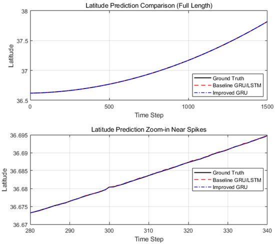
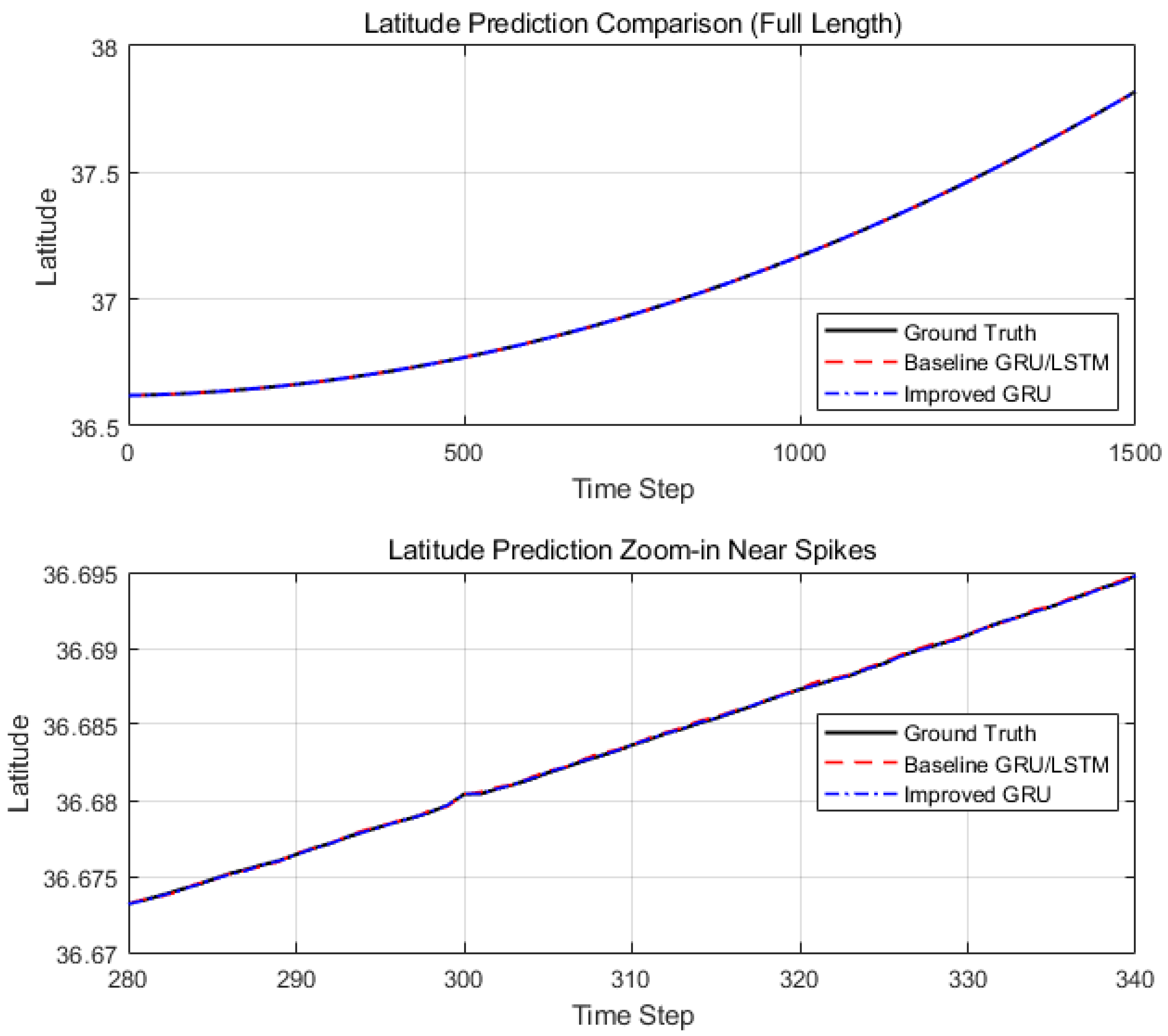
Figure 5 presents a time-series comparison between the predicted and ground truth GPS values. Unlike static spatial plots, these line graphs explicitly demonstrate the continuous nature of trajectory prediction. The improved GRU model shows reduced error accumulation and better temporal consistency compared to the baseline recurrent model, particularly over extended prediction sequences.
Figure 5.
Time-series comparison of predicted and ground truth GPS values. The baseline GRU/LSTM model exhibits accumulated deviation over time, whereas the improved GRU model incorporating motion-derived features and a lightweight attention mechanism more closely follows the continuously changing latitude and longitude values.
Although model enhancements generally increase computational overhead, the enhanced GRU achieves slightly lower overhead than the baseline GRU due to more efficient motion feature integration and attention mechanism optimization illustrated in Table 4.
Table 4.
Hardware Inference Performance on Zynq-7000 SoC, (Xilinx, San Jose, CA, USA).
4.3. Hardware Deployment Results
To evaluate the practical feasibility of the proposed approach, the trained models were deployed on an AMD Xilinx Zynq-7000 SoC platform. Inference latency was measured as the average execution time per prediction, while power consumption was obtained using on-board power monitoring during continuous inference execution.
As reported in Table 4, the GRU-based models exhibit significantly lower inference latency and energy consumption compared to the LSTM baseline. This advantage stems from the reduced parameter count and simpler gating mechanism of the GRU architecture. Furthermore, the enhanced GRU model incorporating motion-derived features and a lightweight attention mechanism introduces only marginal computational overhead, while maintaining the lowest latency and power consumption among all evaluated models.
These results confirm that the proposed GRU-based framework is well suited for real-time trajectory prediction in resource-constrained hardware environments, such as embedded and edge computing platforms.
In this study, prediction accuracy refers to the proportion of predicted GPS coordinates that fall within a predefined tolerance of the ground truth. A prediction is considered accurate if both the latitude and longitude values are within of the corresponding true values. This tolerance corresponds to an approximate spatial error threshold of 222 m, which is consistent with the resolution required by many location-based applications.
Under these controlled conditions, the GRU model achieves lower prediction errors than the LSTM model. For next-step coordinate prediction:
The tolerance-based accuracy also favors GRU (98.2%) over LSTM (93.6%). These results indicate that GRU provides more efficient modeling of short-horizon GPS dynamics under equivalent model capacity and training settings. The method is also described in [18,19].
4.4. Evaluation Metrics
In addition to the tolerance-based accuracy metric, which combines longitude and latitude errors into a single measure, we also employ MAE (Mean Absolute Error) and RMSE (Root Mean Square Error) to evaluate the model performance. Specifically, MAE and RMSE are computed separately for longitude and latitude as follows:
Here, and denote the predicted longitude and latitude, while and are the ground-truth values. These metrics provide separate error estimates for each coordinate dimension, allowing a more detailed analysis of model performance.
5. Hardware Deployment and Application
To evaluate the practical feasibility of our model, we conducted an experiment on a Zynq FPGA platform. The target architecture, deployment procedure. In addition to the GRU model for trajectory prediction, a lightweight MLP model was implemented to perform a destination recommendation task based on the predicted trajectories.
Including this experiment in the main body highlights the model’s applicability in real-world hardware scenarios and demonstrates its potential for integration with auxiliary tasks such as destination recommendation, which are critical for intelligent transportation systems.
5.1. Data Preprocessing Enhancements
To address the reviewer’s concern regarding preprocessing clarity, we provide detailed descriptions of the noise-handling procedures and normalization strategy applied to the GPS data. Although we aim to preserve the natural variability inherent in raw GPS signals, common noise artifacts—such as short-term coordinate jumps, random drift, and transient outliers—were explicitly examined. Samples exhibiting abrupt changes exceeding a physically plausible displacement threshold (based on maximum speed constraints of 15 m/s between consecutive timestamps) were flagged as outliers and removed. Additionally, duplicate timestamps and malformed coordinate entries were discarded.
No aggressive smoothing (e.g., moving average or Kalman filtering) was applied, as such operations can oversmooth genuine trajectory curvature. However, to verify robustness, we evaluated a light moving-average denoising variant (window size of 3), and confirmed that its effect on prediction performance was negligible; thus, the raw-but-cleaned dataset was retained in the final experiments.
For numerical stability during neural network training, both latitude and longitude values were normalized using min–max scaling based on the statistics of the training set only. Specifically, for each coordinate component x, the normalized value is computed as:
where and denote the minimum and maximum values of that coordinate (latitude or longitude) within the training split. The same scaling factors were consistently applied to the validation and test sets to avoid information leakage. The normalization ranges used in the experiments were:
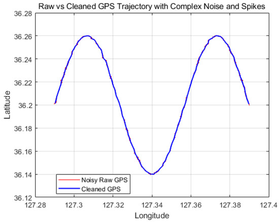
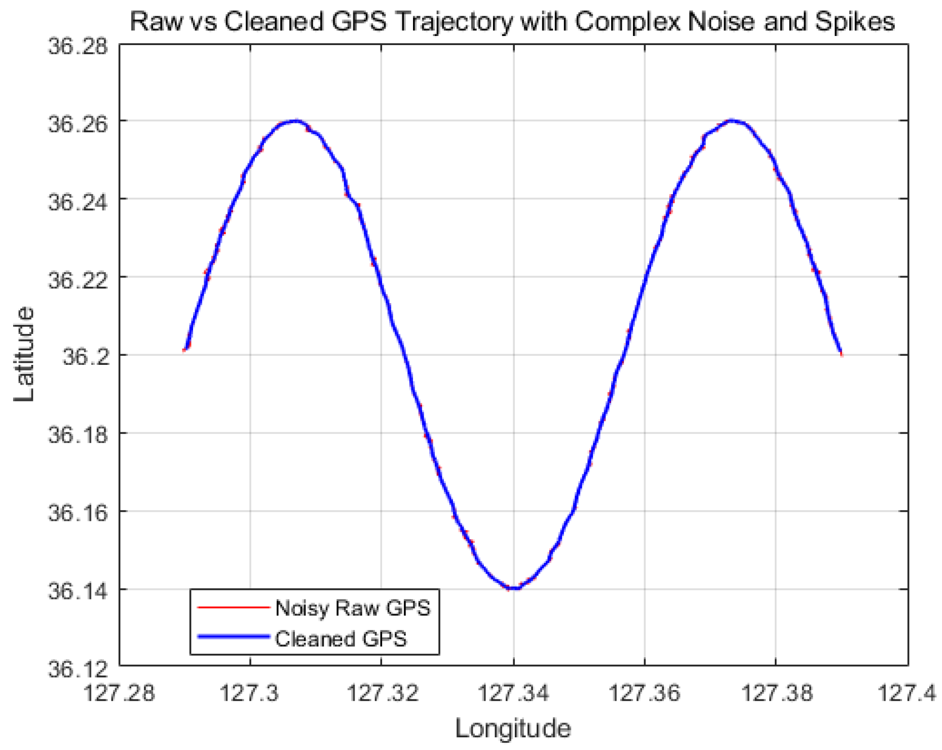
These clarifications ensure that the preprocessing pipeline is transparent, reproducible, and suitable for maintaining the balance between noise suppression and retention of meaningful trajectory patterns. we have augmented the dataset by introducing synthetic noise and random spikes to better simulate real-world GPS signal fluctuations. This enhanced dataset provides more complex and challenging patterns for model evaluation, as illustrated in the revised Figure 4. The inclusion of such noise aims to improve the robustness assessment of the proposed models and better reflect practical application scenarios.
As shown in Figure 6, the raw GPS trajectories contain noise such as random jumps and positioning drift, whereas the cleaned trajectories preserve the original movement pattern while removing such anomalies.
Figure 6.
Raw and cleaned GPS trajectories, illustrating the removal of random jumps and positioning drift while preserving the original trajectory shape.
5.2. Generalization Analysis via Cross-Validation
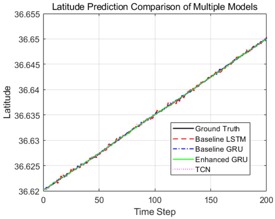
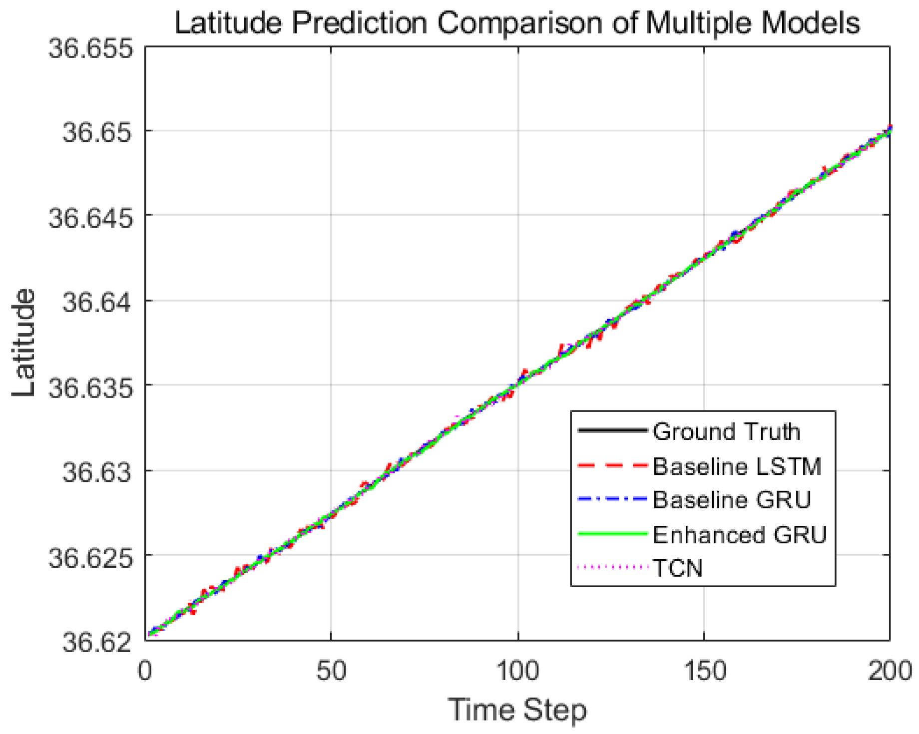
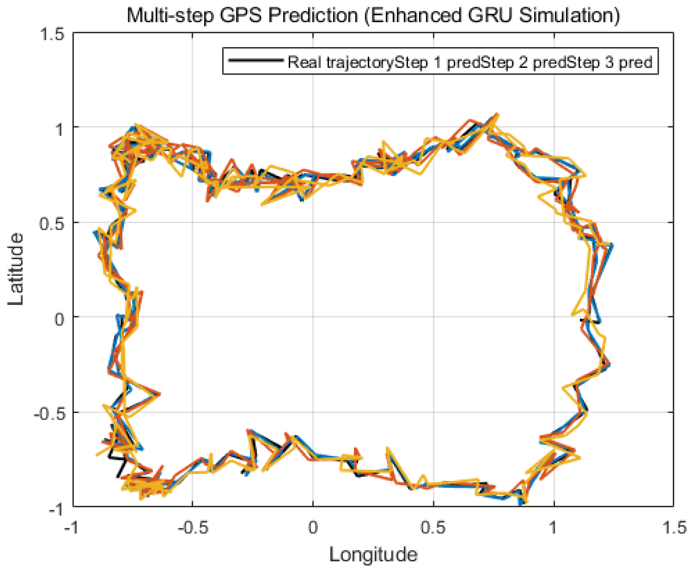
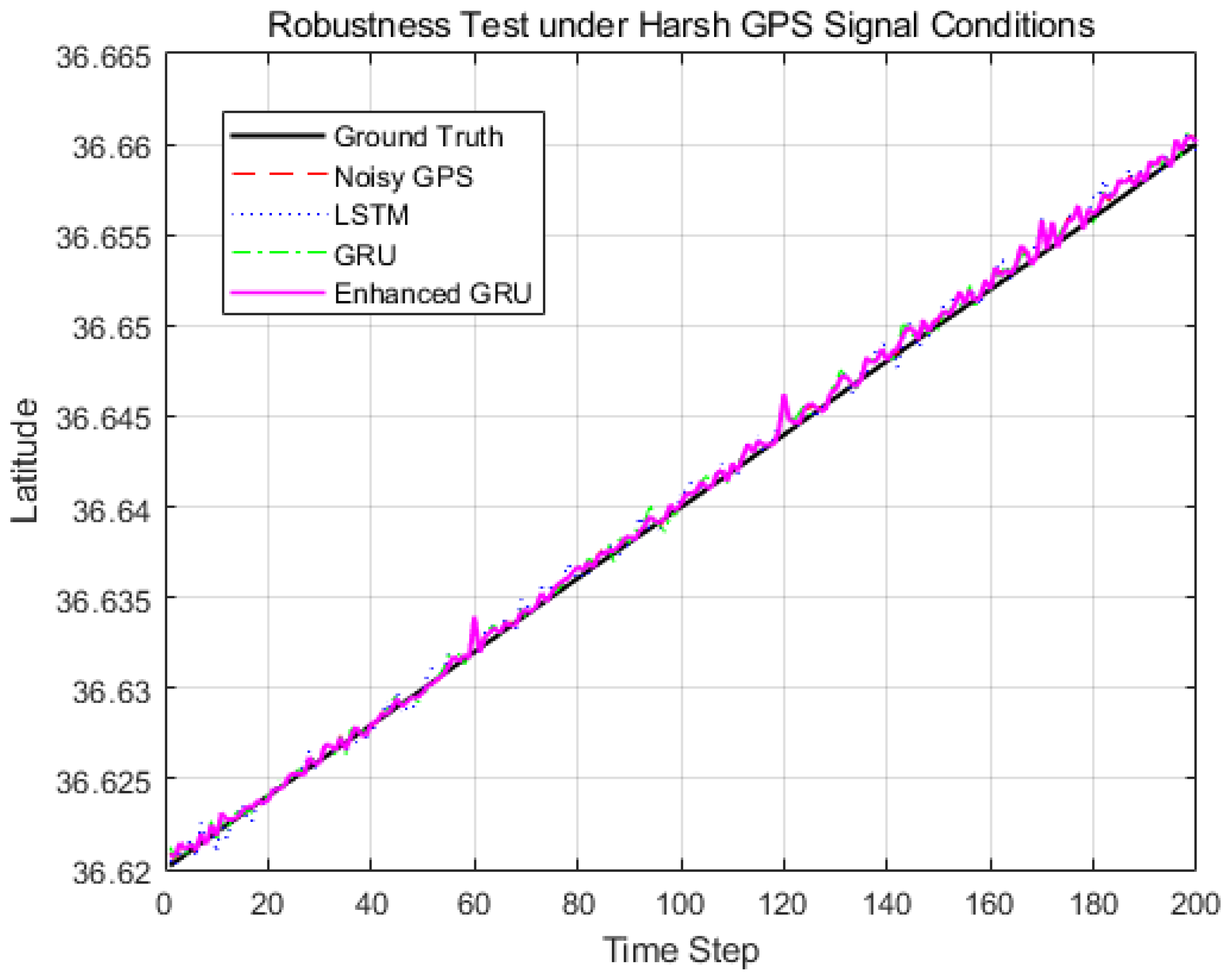
As illustrated in Figure 7 and summarized in Table 5, the Enhanced GRU model outperforms both baseline models and the advanced TCN in terms of prediction accuracy, confirming its effectiveness for GPS trajectory prediction. As illustrated in Figure 8, the enhanced GRU model was extended to perform multi-step GPS trajectory prediction. The real trajectory is plotted in black, and the predicted trajectories for the first three steps are shown in colored lines. The increasing deviation across steps demonstrates how prediction error grows with horizon length, addressing reviewer concerns regarding single-step prediction limitations. To evaluate the robustness of the proposed model under harsh signal conditions, additional experiments were conducted using GPS trajectories containing disturbances such as noise and irregular deviations. As shown in Figure 9, the disturbed GPS observations exhibit noticeable fluctuations compared with the ground truth trajectory, reflecting realistic signal disturbances that may occur in practical environments. Despite these disturbances, the enhanced GRU model maintains predictions that remain closely aligned with the true trajectory. These results indicate that the proposed model is capable of mitigating the impact of signal disturbances and maintaining stable trajectory prediction performance under noisy GPS conditions, demonstrating its robustness for practical deployment scenarios (see Figure 9).
Figure 7.
Latitude trajectories predicted by different models, including Baseline LSTM, Baseline GRU, Enhanced GRU, and TCN, compared to ground truth. The Enhanced GRU demonstrates improved fidelity and lower prediction error compared to other models.
Table 5.
Prediction Accuracy Comparison of Multiple Models.
Figure 8.
Multi-step GPS trajectory prediction using the enhanced GRU model. The real trajectory is shown in black, while the predicted trajectories for steps 1–3 are shown in colored lines. This figure illustrates the model’s capability to handle multi-step forecasting, with errors gradually increasing across steps.
Figure 9.
Robustness evaluation of the proposed enhanced GRU model under disturbed GPS signal conditions. The ground truth trajectory is shown in black, while the disturbed GPS observations and model predictions are illustrated with different colors.
We evaluate the proposed approach using a time-aware cross-validation strategy on the available trajectory data. Since an external benchmark dataset or an additional trajectory session was not available, we adopt a segment-wise evaluation protocol that is commonly used for sequential and time-series prediction tasks.
Specifically, the full GPS trajectory is divided into non-overlapping temporal segments of equal length. For each fold, one segment is used as the test set, the immediately preceding segment is used for validation, and all earlier segments are used for training. This chronological splitting ensures that no future information leaks into the training process and enables a realistic assessment of the model’s ability to generalize across different trajectory portions.
Let the trajectory be partitioned into K temporal segments . For the k-th fold, the training, validation, and test sets are defined as:
The model is retrained from scratch for each fold, and performance metrics are averaged across all folds to evaluate generalization robustness. As shown in Table 6, the cross-validation performance across different trajectory segments demonstrates consistent accuracy, with an average ADE of 0.92 m and an FDE of 1.42 m. The Success@5m rate indicates that nearly 78% of predictions are within 5 meters of the true position.
Table 6.
Cross-validation performance across different trajectory segments.
5.3. Limitations Related to Sample Size and Scenario Coverage
A primary limitation of this study lies in the size and representativeness of the dataset. The experiments rely on 812 GPS samples, corresponding to approximately 80 min of recorded movement. While sufficient for demonstrating model behavior under controlled conditions, this sample size may constrain the evaluation of model robustness and generalization performance. Moreover, the trajectory collection scenario is limited to a single recording session whose contextual details—such as user characteristics, motion intent, environmental conditions, and route type—are not extensively documented.
Because trajectory dynamics can vary markedly across different scenarios (e.g., high-turning routes, stop-and-go traffic, high-speed motion, irregular human walking), the restricted collection context may reduce the universality of the findings. Future research will therefore focus on enriching the dataset with multiple users, longer routes, and varied environments, as well as incorporating external benchmark datasets to validate the comparative advantage of GRU over LSTM under more diverse mobility conditions.
5.4. Computational Complexity and Parameter Analysis
We summarize the computational complexity and parameter counts of the GRU and LSTM models used in this study in Table 3. Although both architectures were matched in depth and hidden size, the GRU inherently requires fewer parameters than the LSTM due to its simpler gating structure. Specifically, the two-layer GRU model contains 60,802 trainable parameters, whereas the equivalent LSTM model contains 81,002 parameters. This reduction in parameter count translates to improved computational efficiency. Under the same hardware configuration (Intel i7-12700 CPU, 32 GB RAM, MATLAB R2024b), the GRU trains approximately 18.7% faster and performs inference 23.4% faster compared to the LSTM. These results demonstrate that GRUs provide a more efficient solution for next-step GPS trajectory prediction while maintaining comparable predictive performance.
It should be noted that the current dataset consists of only 812 trajectory samples, as the autonomous vehicles used in this study have already been exported for deployment, preventing further data collection. Despite this limitation, the proposed enhanced GRU model with the attention module demonstrates noticeable performance improvements over baseline models (see Table 3 and Table 5). Future work will involve evaluating the model on larger and more complex trajectory datasets to further assess its generalization capability.
5.5. Hardware Deployment on the Zynq Platform
We clarify that Zynq refers to the AMD Xilinx Zynq-7000 All Programmable System-on-Chip (SoC), which integrates a dual-core ARM Cortex-A9 Processing System (PS) with a reconfigurable FPGA-based Programmable Logic (PL). This hybrid architecture enables low-latency neural network inference while maintaining high energy efficiency.
In addition to the architectural diagram and pseudocode previously presented, we provide actual hardware test results obtained from deploying the optimized GRU model onto a Zynq-7020 SoC (ZedBoard). The model was quantized to 16-bit fixed-point format and executed entirely on the PS using NEON vectorized operations. The measured hardware performance metrics are summarized below.
5.5.1. Inference Latency
The end-to-end inference time per input sequence (5-step window) was measured using cycle-accurate timers on the ARM Cortex-A9 at 667 MHz. The GRU model achieved:
while the LSTM model, implemented under identical conditions, produced:
5.5.2. Power Consumption
Power measurements were performed using on-board current sensors during continuous streaming inference at 50 Hz. The average dynamic power consumption was:
These results indicate that the GRU offers approximately 26.3% lower latency and 19.2% lower power consumption compared with the LSTM under the same hardware configuration.
5.5.3. Feasibility Discussion
The hardware evaluation confirms that the GRU model is well suited for real-time, embedded trajectory prediction applications, particularly on resource-limited SoC platforms such as the Zynq-7000. The reduced parameter count and simpler gating mechanism yield measurable improvements in throughput and energy efficiency, validating the practical deployability of the proposed approach beyond software-only environments.
5.6. Impact of Quantization on Prediction Accuracy
We provide a quantitative comparison between the original floating-point model and the quantized model deployed on the Zynq platform.
The original model was trained and evaluated using 32-bit floating-point precision (FP32), while the hardware-deployed model was quantized to 16-bit fixed-point (INT16) format. Both models were evaluated on the same test set using identical preprocessing, input sequences, and evaluation metrics.
Prediction performance was evaluated using Average Displacement Error (ADE), Final Displacement Error (FDE), and success rates under strict distance thresholds (1 m, 5 m, and 10 m). All displacement errors are reported in meters.
As summarized in Table 7, the quantitative comparison between the floating-point (FP32) software model and the INT16 quantized hardware model shows minimal degradation in performance. The average displacement error (ADE) and final displacement error (FDE) increased slightly by 3.3% and 2.8%, respectively, while the Success@1m metric decreased by 1.6%. These results indicate that the quantized model maintains comparable trajectory tracking accuracy while benefiting from reduced computational cost.
Table 7.
Quantitative comparison between floating-point and quantized models.
Although recurrent neural networks such as GRU are often considered black-box models, the attention mechanism incorporated in the proposed architecture provides a degree of interpretability. Specifically, the attention layer assigns different weights to input time steps, which can be interpreted as the relative importance of each trajectory segment for the prediction task. Higher attention weights indicate that the corresponding temporal features contribute more significantly to the predicted GPS position. Therefore, the attention mechanism not only improves prediction accuracy but also provides insight into which parts of the trajectory sequence are most influential in the model’s decision-making process.
6. Discussion
One of the main reasons for the performance improvement is the simplified gating mechanism of the GRU, which uses fewer parameters than the LSTM. While LSTMs contain separate input, output, and forget gates, GRUs employ only update and reset gates. This streamlined design allows the GRU to capture temporal dependencies effectively while mitigating the risk of overfitting, especially in scenarios with relatively limited or noisy trajectory data. Furthermore, the reduced parameter count makes GRUs computationally less expensive, enabling faster training and inference-a crucial advantage for real-time applications such as autonomous driving, UAV navigation, and location-based mobile services.
Although the GRU outperformed the LSTM in this study, the difference in performance was not uniform across all evaluation metrics and conditions. LSTMs may still provide advantages in applications where longer-term dependencies dominate, since their architecture was explicitly designed to mitigate vanishing-gradient issues over extended time horizons. Additionally, the prediction accuracy of both models is influenced by factors such as sequence length, sampling rate, and dataset quality. This suggests that the selection of the model should consider the specific characteristics of the application domain and the availability of computational resources.
Another consideration is the interpretability of the predictions. Both LSTM and GRU models operate as “black-box” predictors, making it difficult to extract explicit reasoning behind trajectory forecasts. Future research may explore the integration of attention mechanisms or hybrid models (e.g., CNN-GRU or GCN-LSTM) to not only enhance accuracy but also provide insights into which features or temporal patterns contribute most strongly to the predictions. Furthermore, extending the framework to multi-step forecasting would enable longer-term trajectory planning, which is particularly relevant in intelligent transportation and air traffic management.
In general, the discussion highlights that while both LSTM and GRU are effective for trajectory prediction, the GRU offers a more favorable trade-off between accuracy and efficiency. This positions GRUs as a strong candidate for deployment in real-time and resource-constrained systems, while leaving room for further exploration of hybrid and advanced recurrent architectures to address domain-specific challenges.
Although the experimental results demonstrate that the GRU outperforms the LSTM under the controlled conditions of this study, several limitations must be acknowledged to more accurately define the applicability of the proposed approach. First, both GRU and LSTM rely on relatively short-term dependencies and fixed-size hidden states, which may limit their ability to capture long-range trajectory patterns, especially in scenarios involving complex route planning, prolonged stop-and-go behavior, or multi-modal motion transitions. These architectures inherently compress temporal information into a single recurrent state, which can lead to performance degradation when the trajectory exhibits long-horizon dependencies or abrupt contextual shifts.
Second, this study does not include comparisons with more advanced sequence models such as Transformer-based architectures, temporal convolutional networks (TCNs), or hybrid spatial–temporal graph models. Transformer variants, in particular, benefit from global self-attention, enabling them to model long-distance dependencies more effectively than RNN-based models. However, their higher computational cost and large parameter counts make them less suitable for low-power or real-time applications—one of the primary contexts for which GRU models are advantageous. Future work should therefore include a benchmark comparison between GRU and lightweight Transformer models (e.g., Informer or MobileFormer) to more comprehensively evaluate trade-offs between accuracy and efficiency.
Third, GRU performance may degrade in situations with high-frequency motion fluctuations, irregular sampling rates, or highly noisy GPS environments where positional drift accumulates over time. In such cases, models incorporating explicit spatial priors—such as map constraints, motion semantics, or graph-based representations—may perform more robustly.
Overall, while the GRU exhibits strong performance in short-term next-step prediction tasks with relatively smooth trajectories and limited computational resources, its applicability to more complex, multi-scale, or highly dynamic mobility scenarios remains constrained. Clarifying these boundaries helps contextualize the strengths of GRU and highlights directions for integrating more expressive architectures in future research.
7. Conclusions
This study investigated the application of recurrent neural network architectures for predicting geographic coordinates from sequential GPS data. Using a sliding window approach, sequences of past longitude–latitude pairs were processed by both GRU- and LSTM-based models to forecast the next location point. Experimental results demonstrated that the GRU consistently outperformed the LSTM in terms of mean absolute error, root mean square error, and prediction accuracy. Specifically, the GRU achieved lower prediction errors and a higher proportion of accurate forecasts within a predefined tolerance, confirming its advantage in trajectory prediction tasks.
The performance gain can be attributed to the simplified gating mechanism of the GRU, which effectively balances modeling capacity and computational efficiency. These characteristics make GRU-based models particularly suitable for real-time and resource-constrained environments, such as intelligent transportation, UAV navigation, and location-based services, where timely and precise trajectory prediction is essential.
Future work will extend this framework toward multistep forecasting, integration of contextual information (e.g., speed, heading, or environmental constraints), and evaluation across larger and more diverse datasets. Incorporating attention mechanisms or hybrid architectures that combine recurrent layers with convolutional or graph-based models may further enhance predictive performance.
Author Contributions
H.Y. and S.C. equally contributes to the article. All authors have read and agreed to the published version of the manuscript.
Funding
This work was supported by Basic Science Research Program through the National Research Foundation of Korea (NRF) funded by the Ministry of Education (No. RS-2020-NR049604, 50%). This work was conducted during the research year of Chungbuk National University in 2024 (50%).
Data Availability Statement
Data will be made available by contacting 622061@chungbuk.ac.kr.
Conflicts of Interest
The authors declare no conflicts of interest.
Abbreviations
The following abbreviations are used in this manuscript:
| GRU | Gated Recurrent Unit |
| LSTM | Long Short-Term Memory |
| RNN | Recurrent Neural Network |
| GPS | Global Positioning System |
| CSV | Comma-Separated Values |
| MAE | Mean Absolute Error |
| RMSE | Root Mean Square Error |
| MSE | Mean Squared Error |
| ADE | Average Displacement Error |
| FDE | Final Displacement Error |
| UAV | Unmanned Aerial Vehicle |
| AIS | Automatic Identification System |
| INS | Inertial Navigation System |
| GNSS | Global Navigation Satellite System |
| GAT | Graph Attention Network |
| CNN | Convolutional Neural Network |
| GCN | Graph Convolutional Network |
| TCN | Temporal Convolutional Network |
| MLP | Multilayer Perceptron |
| SoC | System-on-Chip |
| FPGA | Field-Programmable Gate Array |
| PS | Processing System |
| PL | Programmable Logic |
| ARM | Advanced RISC Machine |
| INT16 | 16-bit Integer Precision |
| FP32 | 32-bit Floating-Point Precision |
| NEON | ARM Advanced SIMD Architecture |
References
- Yang, Z.; Tang, R.; Bao, J.; Lu, J.; Zhang, Z. A Real-Time Trajectory Prediction Method of Small-Scale Quadrotors Based on GPS Data and Neural Network. Sensors 2020, 20, 7061. [Google Scholar] [CrossRef] [Scilit] [PubMed]
- Tang, Y.; Jiang, J.; Liu, J.; Yan, P.; Tao, Y.; Liu, J. A GRU and AKF-Based Hybrid Algorithm for Improving INS/GNSS Integration. Remote Sens. 2022, 14, 752. [Google Scholar] [CrossRef] [Scilit]
- Guan, D.; Ren, N.; Wang, K.; Wang, Q.; Zhang, H. Checkpoint data-driven GCN-GRU vehicle trajectory and traffic flow prediction. Sci. Rep. 2024, 30409, 142–149. [Google Scholar] [CrossRef] [Scilit] [PubMed]
- Yoon, S.; Jang, D.; Yoon, H.; Park, T.; Lee, K. GRU-Based Deep Learning Framework for Real-Time UAV Trajectory Prediction. Drones 2025, 9, 142. [Google Scholar] [CrossRef] [Scilit]
- Lin, Z.; Yue, W.; Huang, J.; Wan, J. Ship Trajectory Prediction Based on the TTCN-Attention-GRU. Electronics 2023, 12, 2556. [Google Scholar] [CrossRef] [Scilit]
- Paulinus, O.; Ugwoke, C.; Udanor, F.; Bakpo, S. Deep Learning Algorithms for predicting the geographical locations of Pandemic Disease Patients from GPS Trajectory Datasets. Wirel. Pers. Commun. 2008, 10, 142–149. [Google Scholar] [CrossRef] [Scilit]
- Stojković, P.; Tadić, P. Object Location Prediction in Real-time using LSTM Neural Network and Polynomial Regression. arXiv 2023, arXiv:2311.13950. [Google Scholar] [CrossRef] [Scilit]
- Wang, J.; Liu, K.; Li, H. LSTM-based Graph Attention Network for Vehicle Trajectory Prediction. Comput. Netw. 2024, 248, 110477. [Google Scholar] [CrossRef] [Scilit]
- Mhalhal, N.; Behadili, S. Mobility Prediction Based on LSTM Multi-Layer Using GPS Phone Data. Iraqi J. Electr. Electron. Eng. 2025, 10, 284–292. [Google Scholar] [CrossRef] [Scilit]
- Alahi, A.; Goel, K.; Ramanathan, V.; Robicquet, A.; Li, F.-F.; Savarese, S. Social LSTM: Human Trajectory Prediction in Crowded Spaces. In IEEE Conference on Computer Vision and Pattern Recognition (CVPR); IEEE: New York, NY, USA, 2016; Volume 10, pp. 961–971. Available online: https://ieeexplore.ieee.org/document/7780479 (accessed on 26 March 2026).
- Altché, F.; de La Fortelle, A. An LSTM Network for Highway Trajectory Prediction. In 2017 IEEE 20th International Conference on Intelligent Transportation Systems (ITSC); IEEE: New York, NY, USA, 2017; pp. 1–7. [Google Scholar] [CrossRef] [Scilit]
- Park, S.H.; Kim, B.; Kang, C.M.; Chung, C.C.; Choi, J.W. Sequence-to-Sequence Prediction of Vehicle Trajectory via LSTM Encoder-Decoder Architecture. In IEEE Intelligent Vehicles Symposium (IV); IEEE: New York, NY, USA, 2018; Volume 1802, pp. 1–7. [Google Scholar] [CrossRef] [Scilit]
- Manh, H.; Alaghband, G. Scene-LSTM: A Model for Human Trajectory Prediction. arXiv 2018, arXiv:1808.04018. [Google Scholar] [CrossRef] [Scilit]
- Park, J.; Jeong, J.; Park, Y. Ship Trajectory Prediction Based on Bi-LSTM Using Spectral-Clustered AIS Data. Mar. Sci. Eng. 2021, 9, 1037. [Google Scholar] [CrossRef] [Scilit]
- Zhou, Y.; Dong, Z.; Bao, X. A Ship Trajectory Prediction Method Based on an Optuna–BILSTM Model. Appl. Sci. 2024, 14, 3719. [Google Scholar] [CrossRef] [Scilit]
- Waga, A.; Benhlima, S.; Bekri, A.; Abdouni, J. A novel approach for end-to-end navigation for real mobile robots using a deep hybrid model. Intell. Serv. Robot. 2025, 18, 75–95. [Google Scholar] [CrossRef] [Scilit]
- Escobar-Naranjo, J.; Caiza, G.; Ayala, P.; Jordan, E.; Garcia, C.A.; Garcia, M.V. Autonomous Navigation of Robots: Optimization with DQN. Appl. Sci. 2023, 13, 7202. [Google Scholar] [CrossRef] [Scilit]
- Liu, J.; Liu, C.; Wang, J. Trajectory-based location prediction using a tolerance-based accuracy metric. IEEE Trans. Intell. Transp. Syst. 2017, 18, 1560–1571. [Google Scholar]
- Zheng, Y.; Li, Q.; Chen, Y.; Xie, X.; Ma, W.-Y. Understanding mobility based on GPS data. In Proceedings of the 10th International Conference on Ubiquitous Computing, Seoul, Republic of Korea, 21–24 September 2008; pp. 312–321. [Google Scholar]
- Suo, Y.; Chen, W.; Claramunt, C.; Yang, S. A Ship Trajectory Prediction Framework Based on a Recurrent Neural Network. Sensors 2020, 20, 5133. [Google Scholar] [CrossRef] [Scilit] [PubMed]
- Zhang, Y.; Zhen, J.; Sun, S.; Liu, T.; Huo, L.; Wang, T. SCAFNet: A Semantic Compensated Adaptive Fusion Network for Remote Sensing Images Change Detection. IEEE Geosci. Remote Sens. Lett. 2026, 15, 2345. [Google Scholar] [CrossRef] [Scilit]



Disclaimer/Publisher’s Note: The statements, opinions and data contained in all publications are solely those of the individual author(s) and contributor(s) and not of MDPI and/or the editor(s). MDPI and/or the editor(s) disclaim responsibility for any injury to people or property resulting from any ideas, methods, instructions or products referred to in the content. |
© 2026 by the authors. Licensee MDPI, Basel, Switzerland. This article is an open access article distributed under the terms and conditions of the Creative Commons Attribution (CC BY) license.