Classification of Complex Power Quality Disturbances Using the Kaiser Window S-Transform and Deep Convolutional Neural Networks

Abstract

With the wide use of nonlinear loads, power grids’ power quality problems are becoming more prominent, threatening the stability of power systems seriously. To address these problems, this paper proposes a power quality disturbances (PQD)classification method based on the Kaiser window S-transform (KST) and deep neural networks. Firstly, the Kaiser window S-transform is applied to the processing of PQD signals. Secondly, the Kaiser window control function is modified to adjust the shape of the window, and the window function parameters are automatically optimized according to the maximum energy density to achieve a better time-frequency resolution. Then, deep neural networks are utilized to perform deep feature extraction on the feature vectors of the Kaiser window S-transform. Lastly, a Softmax layer is applied to the extracted features. The results show that the method has excellent classification accuracy and noise resistance: the 99.1% accuracy achieved under 20 dB noise.

1. Introduction

In recent years, power quality (PQ) issues have received widespread attention due to the fact that power networks commonly have a large number of nonlinear loads such as automotive charging piles and various power electronics devices [1]. Additionally, the development of renewable energy like wind and solar power has also a certain impact on the grid signals [2]. The use of multiple loads and energy resources will generate different power quality disturbances (PQD), including complex single and nonlinearly mixed PQD signals [3]. To establish a reliable and safe power supply system, accurate detection and classification of these PQD signals are important to deal with disturbance pollution problems, providing crucial support for real-time monitoring and protection [4,5].

Many detection frameworks have been developed to analyze PQD signals, which generally consist of two parts: time-frequency analysis and PQD classification [6]. Since the features of PQD signals are inconspicuous, time-frequency analysis methods are used to extract characteristics in the time domain or frequency domain. Common methods include the short-time Fourier transform (STFT) [7], Stockwell transform (ST) [8], discrete wavelet transform (DWT) [9], and Gaussian window S-transform(GST). However, the fixed window parameters of the STFT are not adaptive to nonstationary signals, and the DWT is sensitive to noise. As an extension, various window parameter setting methods were proposed for the ST, including adjustable window widths [10,11]. Although the resolution of these improved STs is better, the window parameters under complex PQDs still need to be determined empirically [12]. Therefore, effective methods are needed to automatically adjust the optimal parameters to further improve the time-frequency accuracy of complex PQD signals [13].

In the PQD classification step, different features are first extracted from the time-frequency information and then fed to the classifier [14]. Various classification methods have been proposed, such as decision trees (DTs) [4] and support vector machines (SVMs) [15]. It is worth noting that most of their features are handcrafted statistical features (e.g., skewness, kurtosis) [16]. However, the handcrafted features may lead to the loss of critical information, especially for mixed PQDs. Recently, deep learning methods, particularly convolutional neural networks (CNNs), have gained widespread application due to their automatic feature learning capabilities. Nevertheless, directly inputting massive two-dimensional time-frequency matrices into CNNs introduces significant computational overhead, and balancing computational efficiency with robust noise immunity remains a challenge.

To address this issue, this article first proposes an optimized Kaiser window S-transform (KST). It optimizes different window parameters to improve the time-frequency resolution using maximum energy concentration. Instead of using redundant 2D matrices, a lightweight multi-dimensional feature vector is rationally constructed. Furthermore, an improved one-dimensional deep CNN is proposed to classify these extracted features. Integrating the optimized KST and deep CNN, a classification framework is further proposed to detect and classify various single and composite PQD signals. The main contributions of this paper are summarized as follows.

(1)

Adaptive time-frequency analysis: An improved KST is proposed. Breaking away from traditional empirical parameter settings, a particle swarm optimization (PSO) algorithm is introduced to automatically find the optimal Kaiser window shape on the basis of energy density.

(2)

Lightweight feature extraction: A highly representative six-dimensional feature vector is constructed from the KST output, preserving critical time-frequency characteristics while drastically reducing computational dimensionality.

(3)

Robust deep classification framework: A customized 1D deep CNN integrated with batch normalization is designed. Extensive experiments demonstrate that the proposed framework shows superior performance and excellent noise resistance (achieving 99.1% accuracy under 20 dB noise) compared with state-of-the-art methods.

2. Feature Extraction Algorithm Based on the S-Transform

2.1. S-Transform

The S-transform can be regarded as a generalization of the short-time Fourier transform and wavelet transform, serving as a reversible time-frequency analysis method. It uses phase information from the continuous wavelet transform to perform phase correction on the original wavelet [17]. The output of the S-matrix is a complex matrix of $k\times n$ dimensions, whose matrix expression is as follows

$$S(\tau ,f)=A(\tau ,f)e^{-i\phi \left(\tau ,f\right)}$$

(1)

where $\tau$ denotes the time shift factor; $f$ denotes the signal frequency, $A(\tau ,f)$ denotes the amplitude, and $\phi (\tau ,f)$ denotes the phase. Each row represents the specific frequency of the signal at each sampling point from 0 to $N-1$ at a specific time, and each column represents the frequency component of the signal at a specific time. The continuous S-transform of the signal $x\left(t\right)$ is

$$S(\tau ,f)={{\displaystyle \int }}_{-\infty }^{+\infty }x(t)w(\tau -t,f)e^{-j2\pi f\tau }dt$$

(2)

where $w(\tau -t,f)$ denotes the normalized Gaussian window function, i.e.,

$$w(\tau -t,f)={\displaystyle \frac{\left|f\right|}{\sqrt{2\pi }}}{e}^{{\displaystyle \frac{-{(\tau -t)}^2{f}^2}{2}}}$$

(3)

In practical signal processing, power quality disturbance signals are typically discretely sampled signals. The continuous signal $x\left(t\right)$ is now discretized by collecting $N$ points at a sampling interval of $T$, where $\tau \to jT,f\to {\displaystyle \frac{n}{(NT)}}$. The discrete S-transform expression is then derived as follows

$$\left\{\begin{array}{cc}S[jT,{\displaystyle \frac{n}{NT}}]={\displaystyle \sum _{m=0}^{N-1}X}[{\displaystyle \frac{m+n}{NT}}]e^{-{\displaystyle \frac{2{\pi }^2{m}^2}{n^2}}}{e}^{{\displaystyle \frac{i2\pi mj}{N}}}& n\ne 0\\ S[jT,0]={\displaystyle \frac{1}{N}}{\displaystyle \sum _{m=0}^{N-1}x\left[mT\right]}& n=0\end{array}\right.$$

(4)

where $j$ denotes the index of the discretized time point; $m$ represents the summation variable, corresponding to the frequency domain shift operation in the discrete Fourier transform; $n$ indicates the frequency component index, reflecting the position in the frequency domain analysis; and $X\left[{\displaystyle \frac{m+n}{NT}}\right]$ denotes the discrete Fourier transform of signal $x\left(t\right)$ after frequency shifting

$$X\left[{\displaystyle \frac{m+n}{NT}}\right]={\displaystyle \frac{1}{N}}{\displaystyle \sum _{k=0}^{N-1}x(kT)e^{\frac{-i2\pi (m+n)j}{N}}}$$

(5)

For a given PQD signal sequence, feature extraction can be performed using the S-transform. The rows and columns of the extracted two-dimensional matrix represent frequency features and time features, respectively.

2.2. Kaiser Window S-Transformation

Accurate identification of power quality disturbances relies on the feature information extracted from both the time domain and frequency domain. The Kaiser window offers higher time-frequency resolution than the Gaussian window, thereby reducing information loss. Therefore, this paper replaces the Gaussian window function in the S-transform with the Kaiser window function, yielding the Kaiser S-transform (KST). The formula for the Kaiser window S-transform is as follows

$$KST(\tau ,f)={{\displaystyle \int }}_{-\infty }^{+\infty }x(t)w_k(\tau -t,f)e^{-i2\pi ft}dt$$

(6)

where $w_k(t,f)$ corresponds to the Kaiser window function, whose time-domain expression is as follows

$$w_k(t,f)={\displaystyle \frac{I_0[\beta (f)\sqrt{1-{\left(\frac{t}{T}\right)}^2}]}{I_0[\beta (f)]}},\left|t\right|\le T$$

(7)

$$\beta (f)={\displaystyle \frac{{\xi }_1}{f+{\xi }_2}}$$

(8)

where $\beta (f)$ denotes the control function; ${\xi }_1$ and ${\xi }_2$ represent parameters used to control the shape variation of the Kaiser window, enabling adjustment of its shape to achieve better time-frequency resolution; and $I_0(\cdot )$ corresponds to the first-kind zero-order Bessel function.

Now consider discretizing the window function, defining the discrete form of the Kaiser window function as

$$w_k\left(t,\beta \right)={\displaystyle \frac{I_0\left(\beta \sqrt{1-{\left(1-\frac{2t}{N-1}\right)}^2}\right)}{I_0\left(\beta \right)}}$$

(9)

where $t$ denotes the time variable, $\beta$ denotes the window width adjustment factor, and $N$ denotes the number of sampling points.

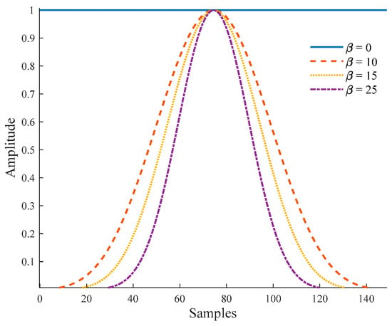
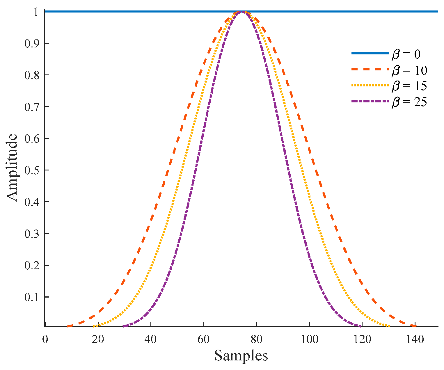
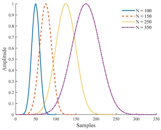
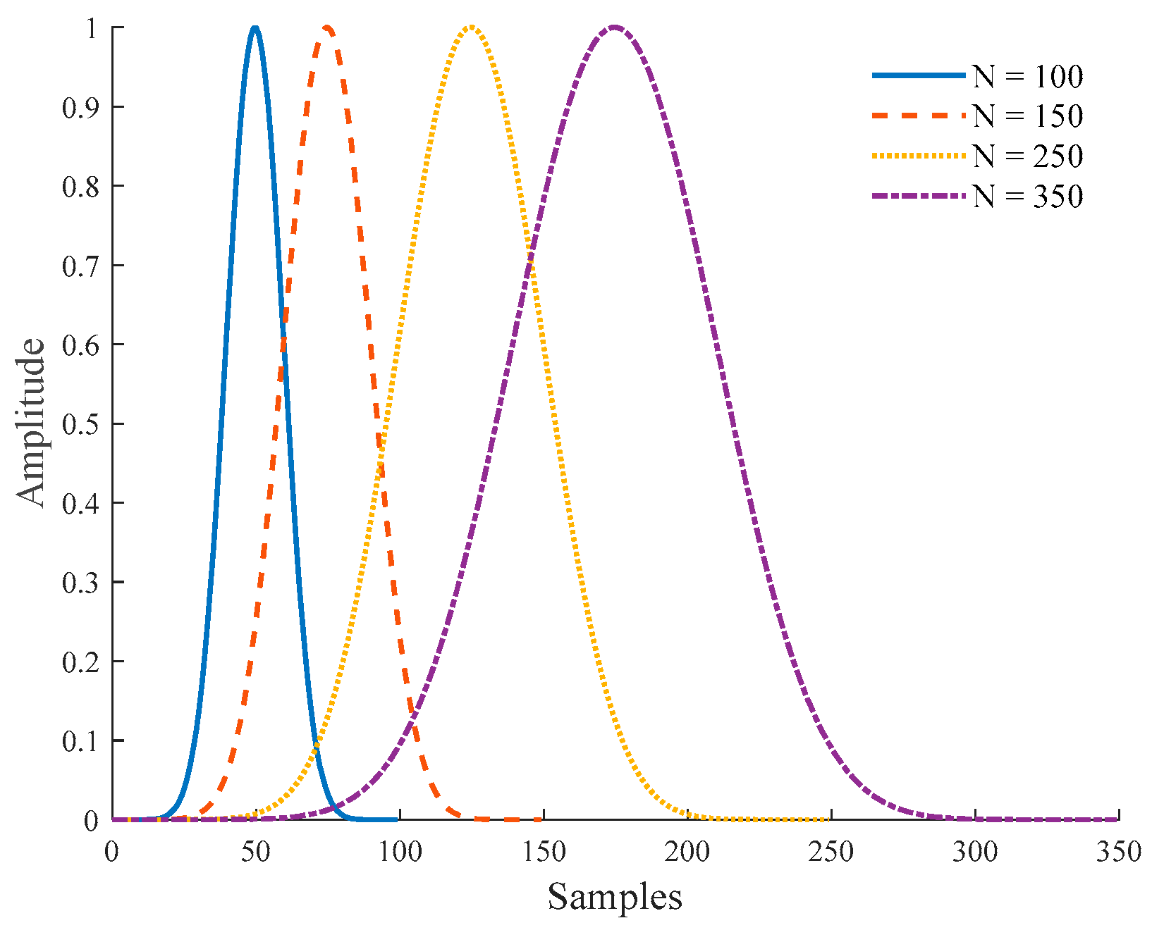
As shown in Figure 1 and Figure 2, the time-domain width of the Kaiser window is influenced by the parameters $\beta$ and $N$, exhibiting a distinct pattern: the window function’s time-domain width decreases as $\beta$ increases, and increases as the number of sampling points increases.

Figure 1. Time-frequency distribution diagram of $\beta$ values ($N$ = 150).

Figure 2. Time-frequency distribution diagram of N values ($\beta$ = 25).

2.3. Improved Kaiser S-Transform

Fixed ${\xi }_1$ and ${\xi }_2$ values cannot accommodate the time-frequency analysis requirements of complex power quality disturbance problems, potentially leading to reduced resolution. To enhance the adaptability of the Kaiser window S-transform to power quality disturbance signals, this paper modifies the control function. Equation (10) presents the new control function $\beta (f)$, which can dynamically adjust the rate of change in window shape by modifying the adjustment factor $\rho$. The new control function is as follows

$$\beta (f)={\displaystyle \frac{{\xi }_1}{(1-\rho )f+{\xi }_2}}$$

(10)

where the value range of $\rho$ is [0, 1). The closer $\rho$ is to 0, the wider the main lobe width of the window function and the weaker the side lobe’s attenuation, making it suitable for applications requiring a broad bandwidth. The closer $\rho$ is to 1, the narrower the main lobe of the window function and the stronger the side lobe’s attenuation, which is suitable for scenarios requiring high-frequency resolution but may simultaneously increase the leakage effect of the window function. Dynamic adjustment of the window shape refers to the real-time adjustment of the value of $\rho$ on the basis of the signal characteristics or processing requirements.

It is worth noting that a single optimized parameter set ($\rho ,{\xi }_1,{\xi }_2$) is sufficient for processing the entire signal duration. The method inherently handles signals where the optimal resolution at the disturbance onset differs significantly from the steady-state portion through the frequency variable $f$ in the control function $\beta (f)$. Because $\beta (f)$ adjusts dynamically with frequency, the Kaiser window automatically narrows for high-frequency transient components (providing high temporal resolution at the disturbance onset) and widens for low-frequency components (ensuring a high frequency resolution during steady states). The optimized parameters simply define the most optimal global shape of this frequency-dependent mapping, eliminating the need for local parameter adaptation over time.

To transition from the continuous Kaiser S-transform to its discrete counterpart, the continuous integration over time is replaced by a discrete summation. Specifically, the continuous time and frequency variables are mapped to discrete integer indices. By applying the discrete convolution theorem alongside Equations (6), (7), (9) and (10), the discrete Kaiser window S-transform’s expression is derived as follows

$$\begin{array}{c}KST(m,n)={\displaystyle \sum _{p=0}^{N-1}X(n+p)W_k(n,\beta )e^{i\frac{2\pi mp}{N}}}\\ =|KST(m,n)|e^{i\psi (m,n)}\end{array}$$

(11)

where $m$, $n$, and $p$ denote integers within the range from 0 to $N-1$ and $m$ is used to alter the time shift, while $p,m$ adjust the translation length of spectrum $x(n)$. $W_k(n)$ and $X(n+p)$ denote the results of the discrete Fourier transform of (7) and $x(t)$, respectively; $|KST(m,n)|$ and $\psi (m,n)$ represent the amplitude and phase of $KST(m,n)$, respectively. $KST(m,n)$ is a matrix of size $L\times W$. Furthermore, to dynamically modify the parameters of the control function $\beta (f)$, the concept of energy density is introduced [18]

$$D_{KST}(\rho ,{\zeta }_1,{\zeta }_2)={\displaystyle \sum _{m=1}^L{\displaystyle \sum _{n=1}^W\left|\frac{KST(m,n)}{\sqrt{\sum \sum |KST(m,n){|}^2}}\right|}}$$

(12)

where $D_{KST}(\rho ,{\zeta }_1,{\zeta }_2)$ denotes the energy density of $KST(m,n)$, where $L$ and $W$ represent the rows and columns of the matrix $KST(m,n)$, respectively.

To achieve maximum energy concentration by adjusting the parameters $\rho$, ${\xi }_1$, and ${\xi }_2$, thereby obtaining the optimal solution, the optimization problem of maximizing the energy concentration can be transformed into finding the minimum solution of the inverse of $D_{KST}(\rho ,{\zeta }_1,{\zeta }_2)$, which can be expressed as

$$\underset{\rho ,{\zeta }_1,{\zeta }_2}{\arg \min }\left\{1/D_{KST}\left(\rho ,{\zeta }_1,{\zeta }_2\right)\right\}$$

(13)

The objective function optimization problem in the formula above is essentially a nonlinear optimization problem. This paper uses a particle swarm optimization (PSO) algorithm to solve it, automatically adjusting the control function parameters for different PQD signals through optimization [19].

To ensure an effective search for the optimal control function parameters, the core parameters of the PSO algorithm are specifically configured. The population size (number of particles) is set to 60, and the maximum number of iterations is limited to 50. The inertia weight is set to 0.7 to maintain a balance between global exploration and local exploitation capabilities. Both the individual learning factor $c_1$ and the social learning factor ($c_2$) are set to 1.5. Furthermore, the search boundaries for the optimization variables $\rho$, ${\xi }_1$, and ${\xi }_2$ are constrained within the ranges of $[0.0,0.95]$, $[0.1,100]$, and $[0.01,10]$, respectively.

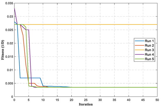
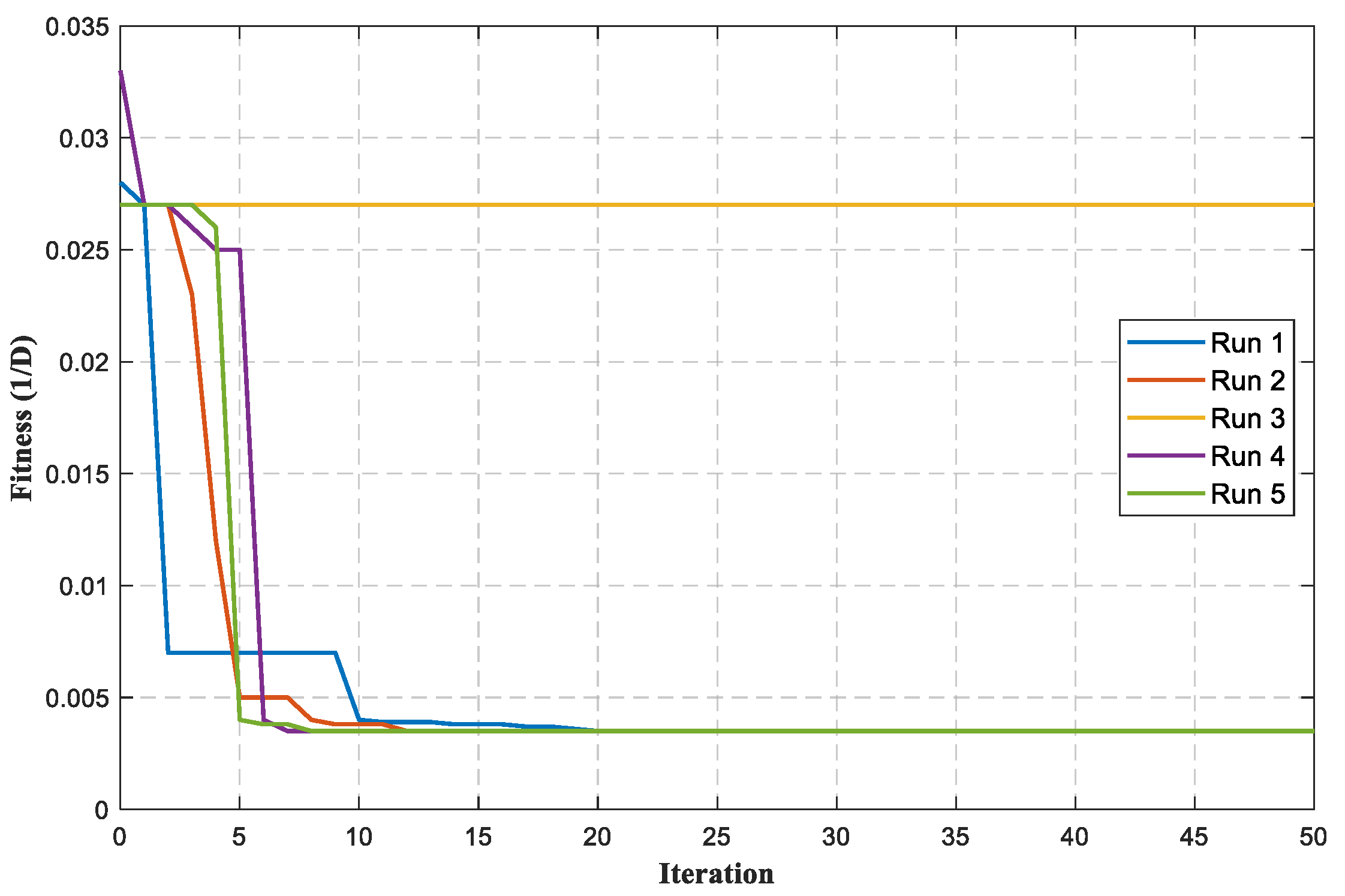
Figure 3 illustrates the optimization convergence curve for maximizing the energy density (represented by minimizing the fitness value $1/D$) under a complex composite disturbance scenario. As shown in the curve, the fitness value drops significantly and the algorithm converges rapidly within the first 15 iterations, demonstrating strong robustness against premature convergence to local minima. The optimal parameter combination obtained from this representative run is $\rho =0.0$, ${\xi }_1=0.80$, and ${\xi }_2=0.01$, achieving a minimum fitness value of approximately 0.0035. This validates the effectiveness of the PSO method in dynamically capturing the optimal time-frequency resolution.

Figure 3. Optimization convergence curve of the PSO algorithm.

Regarding the computational overhead, the time complexity of the PSO optimization process is $O(N\times K\times T_{KST})$, where $N$ is the number of particles, $K$ is the number of iterations, and $T_{KST}$ represents the computational time of a single KST operation. Although the iterative parameter search introduces additional computational load during the initial feature extraction stage, this optimization primarily functions as an offline calibration or a periodic updating process for specific signal patterns. Once the optimal parameters ($\rho$, ${\xi }_1$, ${\xi }_2$) are identified, they are fixed and directly applied to subsequent online data processing. Therefore, this optimization mechanism does not compromise the real-time classification performance of the model in practical engineering applications.

The sampling frequency is set to 6.4 kHz, with a reference frequency of 50 Hz.

2.4. Selection of Eigenvectors

The time-frequency distribution matrix generated by processing PQD signals via the KST algorithm encompasses multi-dimensional key features including disturbance onset/offset times, amplitude modulation, phase shift, event duration, and fundamental frequency fluctuations, revealing the transient response characteristics of nonstationary signals. However, high-dimensional time-frequency features pose challenges for subsequent classification processes. To address this, this paper constructs a multi-dimensional feature vector integrating time-domain and frequency-domain characteristics based on the time-frequency response curves generated by the KST algorithm. This approach significantly reduces computational complexity while maintaining classification accuracy. The feature vector used for identification and classification in this study is as follows

$$\mathit{V}=\left[A_1{A}_2{A}_3{F}_1{F}_2{F}_3\right]$$

(14)

where $A_1$, $A_2$, and $A_3$ denote the maximum amplitude, minimum amplitude, and variance of the time-frequency curve, respectively; $F_1$, $F_2$, and $F_3$ denote the frequencies corresponding to the maximum amplitude, minimum amplitude, and amplitude variance, respectively.

The selection of these specific features is based on the following physical criteria.

Amplitude Features ($A_1$, $A_2$, and $A_3$): These parameters capture the energy envelope and magnitude fluctuations of the signal. They are essential for identifying voltage sags (N2), swells (N1), interruptions (N4), and flickers (N6). For instance, $A_3$ provides a quantitative measure of the severity of voltage fluctuations in composite disturbances.

Frequency Features ($F_1$, $F_2$, and $F_3$): These capture the spectral distribution and frequency-domain stability. They serve as the primary discriminants for harmonics (N3), transient oscillations (N7), and high-frequency components in composite events.

By extracting these six core dimensions, the proposed method reduces the input size for the deep CNN, significantly speeding up the training process without losing critical time-frequency information.

To reduce the classification time in subsequent network operations, the feature vector $\mathit{V}$ must undergo normalization processing before being input into the deep CNN.

3. Classification of Power Quality Disturbance Signals

3.1. Improved Deep CNN

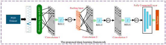
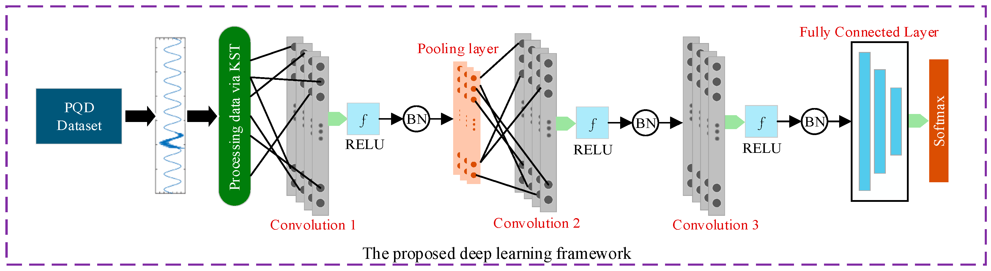
Since the feature vector $\mathit{V}$ is inherently one-dimensional, one-dimensional filters were added throughout the one-dimensional deep CNN in this paper to classify interference. To simultaneously consider local and global features, the filter kernels were constructed to be small, and short strides were adopted in the filters, i.e., VGG-Net. To highlight the PQD features and reduce dimensionality, pooling layers are used before each set of convolutional layers. Additionally, to enhance generalization and mitigate overfitting, batch normalization layers are incorporated at the network’s end. Figure 4 illustrates the proposed deep CNN architecture for automatic classification of PQD signals.

Figure 4. Improved deep CNN architecture.

The one-dimensional convolutional layer, as the core component of the method, enables self-learning feature extraction from perturbed signals. It uses a shared weight filter allocation mechanism and a small receptive field design. Let $X_i$ denote the input $\left(n\times 1\right)$ to the one-dimensional convolutional matrix, $f_s$ denote the number of filters, and $C\left(c\times 1\right)$ denote the dimension of the filter kernel. The formula for the output filter layer $f_s$ from the convolutional layer is as follows

$$X_{0,f_s}^l=f\left({\displaystyle \sum _{i\in n}{X}_i^{K-1}\times C_{io,f_s}^l}+D^L\right)$$

(15)

where $f\left(x\right)$ and $n=m\left(k\times 1\right)$ denote the activation function responsible for the nonlinear activation from the input to output neurons. In the proposed deep neural network, a 64 × 1 convolution kernel is used in the first convolutional layer to enhance noise resistance. The convolution utilizes a 3 × 1 network architecture, focusing on extracting features from local perturbations. Given the limited dimensionality of PQD data, PQD data acquisition uses KST across multiple cycles and sampling points. Consequently, the network architecture is streamlined to comprise a convolutional layer, a pooling layer, a batch normalization layer, a fully connected layer, and a Softmax layer. Through parameter tuning, the proposed one-dimensional network achieves greater simplicity with fewer parameters. Thus, the proposed network is more suitable for classification tasks, imposes lower demands on device performance, and enables faster training speeds.

Batch normalization (BN), a critical component of deep CNNs, effectively suppresses overfitting and enhances training efficiency. Typically deployed after convolutional or fully connected layers and before activation functions, its computation proceeds as follows

$$S_i=\gamma \times {\displaystyle \frac{x_i-{\mu }_m}{\sqrt{{\sigma }_m^2+\epsilon }}}+\beta$$

(16)

where ${\mu }_m$ denotes the mean of the input sample $x_i$, ${\sigma }_m^2$ represents the variance, $\gamma$ is the scaling factor, $\beta$ is the offset, and $\epsilon$ is the correction term to prevent numerical overflow. In PQD classification tasks, optimization algorithms significantly impact reducing training loss and improving classification accuracy. Optimizers play a crucial role in the training process of deep neural networks. Different optimization algorithms have a significant impact on the convergence speed, stability, and final classification performance of the model. With reference to [9], the Adam optimizer is selected in this paper.

3.2. Disturbance Signal Classification

Figure 5 shows the proposed PQD classification method based on KST and thedeep CNN. The proposed method comprises a convolutional layer, a pooling layer, a batch normalization layer, a fully connected layer, and a Softmax layer. Compared with the conventional approach, the proposed classification framework offers the advantage of extracting features through both signal processing and deep CNN layers.

Figure 5. Comparison chart of traditional methods and the classification method in this paper.

4. Case Study Analysis

4.1. Experimental Preparation and Data Acquisition

To evaluate the classification performance of the proposed KST-based and deep CNN-based PQD classification method, this section presents a series of simulations under different levels of noise interference. Based on the IEEE-1159 [20] power quality detection standard and Reference [21], 22 types of power quality disturbances are proposed, including 7 distinct single power quality disturbance signals and 15 composite power quality disturbance signals. The seven distinct single-type PQ disturbance signals are listed in Table 1. All 22 PQ disturbance signals were simulated in MATLAB R2023b. The fundamental frequency was set to 50 Hz, with a signal sampling period of 200 ms and a sampling frequency of 6.4k Hz. Each power quality disturbance comprised 1280 sampling points. The total number of power quality disturbance labels was 22, with each disturbance type having 1000 sample labels. The model described in this paper is built using the TensorFlow framework and Python; see Table 2 for details on the hardware version and runtime environment used.

Table 1. PQD signal model.

Disturbance Signal	Equation	Model Parameters
Swell	$x(t)=\{1+\alpha [\epsilon (t-t_1)-\epsilon (t-t_2)]\}\sin ({\omega }_{0}t)$	$0.1\le \alpha \le 0.8,T\le t_2-t_1\le 9T$
Sag	$x(t)=\{1-\alpha [\epsilon (t-t_1)-\epsilon (t-t_2)]\}sin({\omega }_{0}t)$	$0.1\le \alpha \le 0.9,T\le t_2-t_1\le 9T$
Harmonic	$x(t)=\sin ({\omega }_{0}t)+{\displaystyle \sum _{i=2}^n{k}_i\sin (i{\omega }_{0}t)}$	$0.05\le k_i\le 0.3,i=3,5,7$
Interruption	$x(t)=\{1-\alpha [\epsilon (t-t_1)-\epsilon (t-t_2)]\}\sin ({\omega }_{0}t)$	$0.9\le \alpha \le 1,T\le t_2-t_1\le 9T$
Impulsive transient	$x(t)=\sin ({\omega }_{0}t)+\alpha [\epsilon (t-t_1)-\epsilon (t-t_2)]$	$1\le \alpha \le 3,1\mathrm{ms}\le t_2-t_1\le 3\mathrm{ms}$
Flicker	$x(t)=\left[1+\alpha \left(\sin (\beta {\omega }_{0}t)\right)\right]\sin ({\omega }_{0}t)$	$0.1\le \alpha \le 0.2,0.1\le \beta \le 0.5$
Oscillatory transient	$\begin{array}{l}x\left(t\right)=\sin \left({\omega }_{0}t\right)+\\ \alpha {\mathrm{e}}^{((t_1-t)/\tau )}\sin \left({\omega }_n\left(t-t_1\right)\right)\left[\epsilon \left(t-t_1\right)-\epsilon \left(t-t_2\right)\right]\end{array}$	$\begin{array}{l}1\le \alpha \le 3,3\mathrm{ms}\le \tau \le 50\mathrm{ms},\\ 0.5T\le t_2-t_1\le 3T\\ {\omega }_n=2\pi f_n,700\mathrm{Hz}\le f_n\le 1600\mathrm{Hz}\end{array}$

Table 2. Hardware version and operating environment.

Hardware/Software	Model/Version	Manufacturer Name	Manufacturer Location
OS	Win10 64bit	Microsoft (China) Co., Ltd.	Beijing, China
CPU	Intel i5-8300H	Intel (China) Co., Ltd.	Shanghai, China
RAM	DDR4 16 GB	Kingston Technology (China) Co., Ltd.	Beijing, China
GPU	GTX 1050 4 GB	NVIDIA Semiconductor Technology (Shanghai) Co., Ltd.	Shanghai, China
Python	3.8	Python Software Foundation (China Community)	Beijing/Shanghai, etc.
TensorFlow	2.4.0	Google Information Technology (China) Co., Ltd.	Beijing, China
CUDA	11	NVIDIA Semiconductor Technology (Shanghai) Co., Ltd.	Shanghai, China
cuDNN	8.0.1	NVIDIA Semiconductor Technology (Shanghai) Co., Ltd.	Shanghai, China

The 15 types of composite disturbances (N8–N22) are generated by the linear superposition of the individual disturbance models defined in Table 1 on the same time axis. Both disturbances share the same fundamental frequency and sampling points. This ensures that the physical characteristics of multiple events are preserved simultaneously.

By permuting and combining the 7 individual disturbance signals, 15 composite disturbance signals can be generated. This section simulates a total of 22 power quality disturbance signals, as shown in Table 3.

Table 3. Types of PQD signals.

Marker	Disturbance Type	Marking	Disturbance Type
N1	Swell	N12	Flicker + sag
N2	Sag	N13	Flicker + swell
N3	Harmonic	N14	Flicker + harmonic
N4	Interruption	N15	Oscillatory transient + sag
N5	Impulsive transient	N16	Oscillatory transient + swell
N6	Flicker	N17	Flicker + harmonic + sag
N7	Oscillatory transient	N18	Flicker + harmonic + swell
N8	Harmonics + sag	N19	Harmonic + oscillatory transient + sag
N9	Harmonics + swell	N20	Harmonic + oscillatory transient + swell
N10	Interruption + harmonics	N21	Harmonic + oscillatory transient + interruption
N11	Oscillatory transient + harmonics	N22	Harmonic + oscillatory transient + flicker

4.2. Analysis of Model Recognition Accuracy in the Absence of Noise Interference

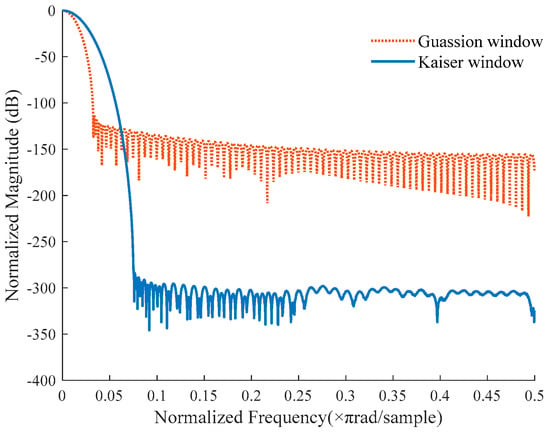
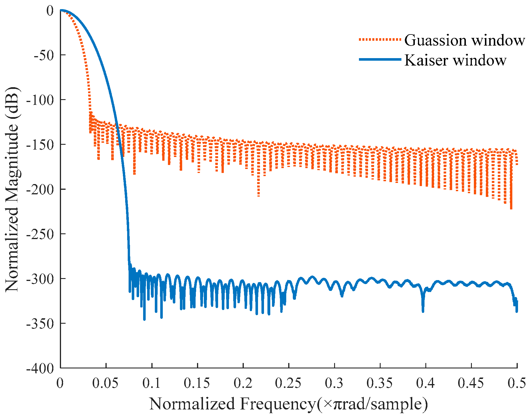
To validate the enhanced time-frequency performance of the improved Kaiser window S-transform in detecting power quality disturbances, the frequency responses of the modified Kaiser window function (11) and the Gaussian window were analyzed. The results are shown in Figure 6.

Figure 6. Spectral characteristics of different window functions.

As shown in Figure 6, at the same detection frequency, the Kaiser window demonstrates superior side lobe suppression performance compared with the Gaussian window, significantly reducing spectral leakage effects. This characteristic enhances the temporal localization accuracy of time-frequency analysis, thereby providing a more precise quantitative basis for signal amplitude detection.

To validate the superiority of the modified Kaiser window S-transform in detecting power quality disturbances, both the modified Kaiser window S-transform and the Gaussian window S-transform were used to identify seven types of power quality disturbance signals (N1–N7) under noise-free conditions. The recognition accuracy rates of the two methods were then compared. The results are shown in Table 4.

Table 4. Recognition results of ST using different window functions.

Category	Accuracy/%
	Improved Kaiser Window S-Transform	Gaussian Window S-Transform
N1	100	98.7
N2	99.7	98.4
N3	99.7	98.6
N4	100	98.3
N5	99.7	97.8
N6	100	98.5
N7	99.8	97.1

The results indicate that the improved Kaiser window S-transform achieves higher accuracy in identifying power quality disturbances compared with the Gaussian window S-transform.

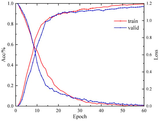
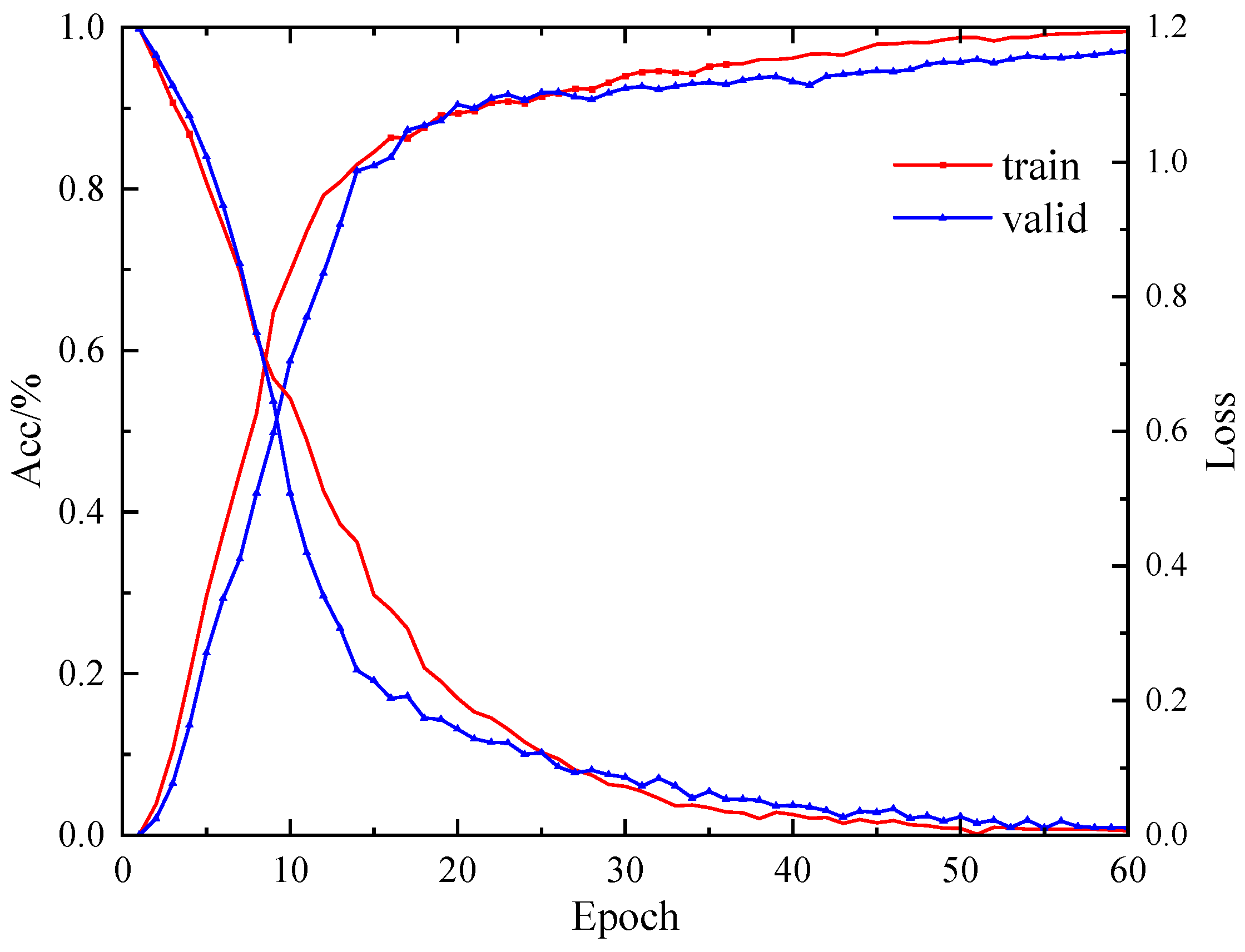
To evaluate the model’s performance in classifying power quality disturbance signals, Figure 7 displays the training process curves for accuracy and loss values. The training results indicate that the model converged after 55 iterations, achieving 99.1% accuracy with a loss value of 0.09. The accuracy curves for the training and validation sets nearly overlap, demonstrating that the model exhibits no overfitting and possesses strong generalization capabilities.

Figure 7. Accuracy and loss value curve.

4.3. Analysis of Classification Performance

4.3.1. Analysis of Classification Performance Under Different Noise Conditions

The signal-to-noise ratio is a metric used to quantify the relative relationship between signal strength and background noise levels. It represents the ratio of useful signal to noise, typically measured in decibels (dB). The fundamental formula for calculating the signal-to-noise ratio is as follows

$$S_{NR}=10\cdot \lg \left({\displaystyle \frac{P_{signal}}{P_{noise}}}\right)$$

(17)

where $S_{NR}$ represents the signal-to-noise ratio, $P_{signal}$ represents the average power of the signal, and $P_{noise}$ represents the average power of the noise.

The signal-to-noise ratio directly impacts signal quality. A high signal-to-noise ratio indicates that the signal is stronger than the noise, making processing easier; a low signal-to-noise ratio may lead to signal distortion. To validate the effectiveness of the model proposed in this paper under different power quality disturbances, we evaluated its noise resistance in extreme noise scenarios such as 40 dB, 30 dB, and 20 dB, as shown in Table 5.

Table 5. Classification accuracy under different noise conditions.

Category	Accuracy/%
	No Noise	40 dB	30 dB	20 dB
N1	100	100	100	100
N2	99.7	99.56	99.43	99.36
N3	99.7	99.65	99.33	99.25
N4	100	99.83	99.43	99.29
N5	99.7	99.53	99.36	99.3
N6	100	99.75	99.47	99.35
N7	99.8	99.66	99.63	99.49
N8	99.75	99.5	99.32	99.17
N9	99.76	99.61	99.35	99.17
N10	99.98	99.75	99.03	98.89
N11	99.83	98.8	98.79	98.71
N12	99.69	99.42	99.31	99.26
N13	99.78	99.59	99.31	99.17
N14	99.7	99.26	99.16	99.04
N15	99.65	98.51	98.47	98.38
N16	99.84	99.41	99.26	99.08
N17	99.57	99.18	98.89	98.73
N18	99.85	99.68	99.51	99.39
N19	99.65	99.46	99.4	99.27
N20	99.62	99.48	99.33	99.15
N21	99.33	99.26	99.14	99.05
N22	99.7	99.54	99.35	99.19

The results indicate that the model’s classification performance is superior in noise-free conditions compared with noisy conditions, and its classification accuracy for single disturbance signals is higher than for composite signals.

To verify the stability of the proposed model, Table 6 presents the variance and standard deviation under different noise conditions.

Table 6. Variance and standard deviation under different noise conditions.

Category	Variance				Standard Deviation
	No Noise	40 dB	30 dB	20 dB	No Noise	40 dB	30 dB	20 dB
N1	0.00021	0.000441	0.001731	0.001239	0.0145	0.021	0.0416	0.0352
N2	0.000306	0.00064	0.000751	0.002323	0.0175	0.0253	0.0274	0.0482
N3	0.00011	0.000713	0.000767	0.001274	0.0105	0.0267	0.0277	0.0357
N4	0.000253	0.00119	0.000841	0.001576	0.0159	0.0345	0.029	0.0397
N5	0.000353	0.001369	0.001592	0.002016	0.0188	0.037	0.0399	0.0449
N6	0.000562	0.000357	0.002172	0.001739	0.0237	0.0189	0.0466	0.0417
N7	0.000144	0.000416	0.001116	0.003306	0.012	0.0204	0.0334	0.0575
N8	0.000156	0.000876	0.001706	0.001954	0.0125	0.0296	0.0413	0.0442
N9	0.000313	0.000372	0.000751	0.001537	0.0177	0.0193	0.0274	0.0392
N10	0.00038	0.000708	0.001122	0.00256	0.0195	0.0266	0.0335	0.0506
N11	0.000266	0.000576	0.002034	0.002916	0.0163	0.024	0.0451	0.054
N12	0.00018	0.00087	0.00149	0.003516	0.0134	0.0295	0.0386	0.0593
N13	0.000408	0.000566	0.00245	0.001332	0.0202	0.0238	0.0495	0.0365
N14	0.000253	0.001096	0.000876	0.002275	0.0159	0.0331	0.0296	0.0477
N15	0.00011	0.000986	0.001962	0.00252	0.0105	0.0314	0.0443	0.0502
N16	0.000497	0.00059	0.001823	0.002581	0.0223	0.0243	0.0427	0.0508
N17	0.000328	0.000734	0.002134	0.003758	0.0181	0.0271	0.0462	0.0613
N18	0.000276	0.00098	0.000756	0.002916	0.0166	0.0313	0.0275	0.054
N19	0.000365	0.001436	0.002088	0.001722	0.0191	0.0379	0.0457	0.0415
N20	0.000237	0.000986	0.000702	0.0022	0.0154	0.0314	0.0265	0.0469
N21	0.000154	0.000412	0.000751	0.003136	0.0124	0.0203	0.0274	0.056
N22	0.000139	0.000529	0.001253	0.003493	0.0118	0.023	0.0354	0.0591

The statistical results show that the standard deviation and variance across all noise conditions are generally low, indicating that the model’s outputs are concentrated and exhibit strong repeatability and consistency. The dispersion is exceptionally low under noise-free and high SNR conditions, confirming stable recognition performance in ideal and mildly noisy environments.

Moreover, the standard deviations for most categories remain low regardless of the noise background, demonstrating the model’s adaptability to external disturbances and its overall noise robustness. Despite minor variations between categories, the limited overall fluctuation proves that the model delivers not only high average recognition accuracy but also reliable and consistent results.

To further validate the superiority of the proposed method within deep learning frameworks, comparative experiments were conducted using two typical models widely applied in power quality disturbance recognition: a CNN-LSTM hybrid model and a temporal convolutional network (TCN). To ensure experimental fairness, all models shared the exact same dataset, training–testing partitions, and input features. Specifically, the feature vectors extracted by the proposed KST algorithm served as inputs for all models, which were subsequently trained and tested under identical parameter configurations. The classification experiments were performed on 22 classes of power quality disturbance signals across different signal-to-noise ratio (SNR) levels, with the accuracy results detailed in Table 7.

Table 7. Classification accuracy across models.

Category	Accuracy/%
	40 dB	30 dB	20 dB
SVM	92.9	92.3	90.2
ELM	95.2	94.7	93.6
kNN	95.6	94.4	93.2
DT	95.9	94.8	93.6
CNN-LSTM	98.7	98.2	97.6
TCN	98.3	97.8	97.2
This Model	99.5	99.4	99.1

To ensure a fair and rigorous comparison, all baseline models (SVM, ELM, kNN, and DT) were carefully optimized to achieve their optimal performance before being compared with the proposed model. We used a five-fold cross-validation combined with a grid search to fine-tune the hyperparameters of each baseline algorithm. Specifically, for SVM, the radial basis function kernel was utilized. The penalty parameter C and kernel coefficient gamma were searched and optimized within $\left\{{10}^{-2},{10}^{-1},1,10,100\right\}$ and $\left\{{10}^{-3},{10}^{-2},{10}^{-1},1\right\}$, respectively. For kNN, the optimal number of neighbors (k) was dynamically tuned within the range of [3,15], and the Euclidean distance metric was selected. For ELM, the number of hidden layer nodes was incrementally searched from 50 to 500 to find the best balance between accuracy and training time, utilizing the Sigmoid activation function. For the DT (Decision Tree), the Gini impurity was used as the splitting criterion, and the maximum depth of the tree was tuned to prevent overfitting. With these equivalent optimization efforts applied to all comparison methods, the intrinsic advantages of the proposed KST-CNN approach in handling complex noisy environments can be fully and objectively shown.

The proposed model is compared with SVM, ELM, kNN, and DT in terms of classification accuracy. The results indicate that when confronted with up to 22 complex power quality disturbances and strong noise interference, the accuracy of traditional SVM and KNN models declines. In contrast, the proposed model maintains high classification accuracy under 20–40 dB noise conditions and demonstrates superior noise robustness. In a 20 dB noisy environment, the accuracy of the proposed model decreased by only 0.4% compared with the noise-free condition, whereas the decline in the comparison methods was at least 1.6%. This demonstrates that the proposed model exhibits superior noise robustness and outperforms other comparison models.

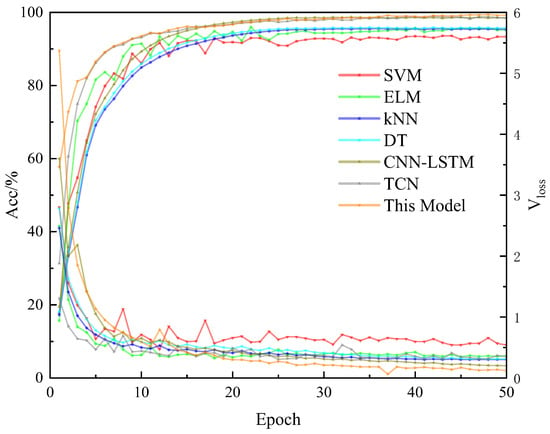
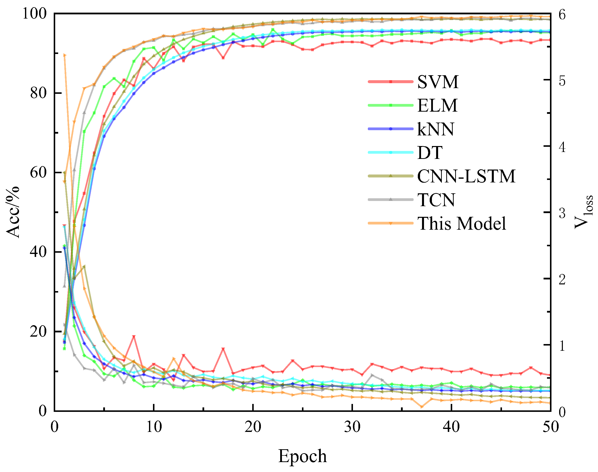
In the experimental phase, all models shared the identical network architecture and training dataset, utilizing a learning rate of 0.00001, a batch size of 128, and a maximum of 50 training epochs. The evaluations were performed under a 40 dB signal-to-noise ratio (SNR). Figure 8 depicts the training processes of the respective models.

Figure 8. Training curves of different models.

As shown in the figure, the proposed KST-CNN model achieved the highest classification accuracy when compared with other methods. These results indicate that by leveraging KST time-frequency feature optimization and a deep CNN structural design, the proposed method effectively improves the recognition of complex power quality disturbance signals while demonstrating superior anti-noise performance.

4.3.2. Comparative Analysis of Different Feature Sets

To verify the optimality of the selected 6D feature set, we conducted comparative experiments against a simplified 3D set (amplitudes only) and an expanded 12D set (including skewness, kurtosis, and energy concentration). The results are shown in Table 8.

Table 8. Comparison of classification performance with different feature dimensions.

Feature Set	Dimensions	Accuracy (20 dB)	Training Time (s)
Amplitude-only set	3	92.5%	42
Proposed set	6	99.1%	48
Extended statistical set	12	99.2%	75

As shown in Table 8, while the 12D set offers a marginal accuracy improvement (0.1%), it nearly doubles the computational time. The proposed 6D feature vector achieves 99.1% accuracy with significantly lower complexity, proving that it is the most efficient choice for real-time power quality monitoring in new power systems.

4.4. Accuracy at Different Training Sample Sizes

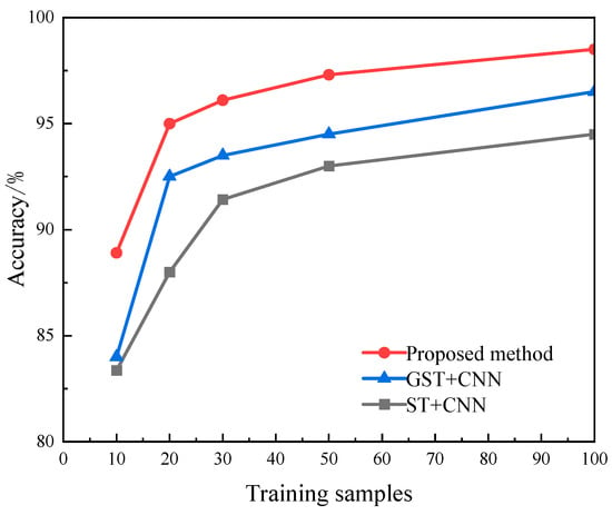
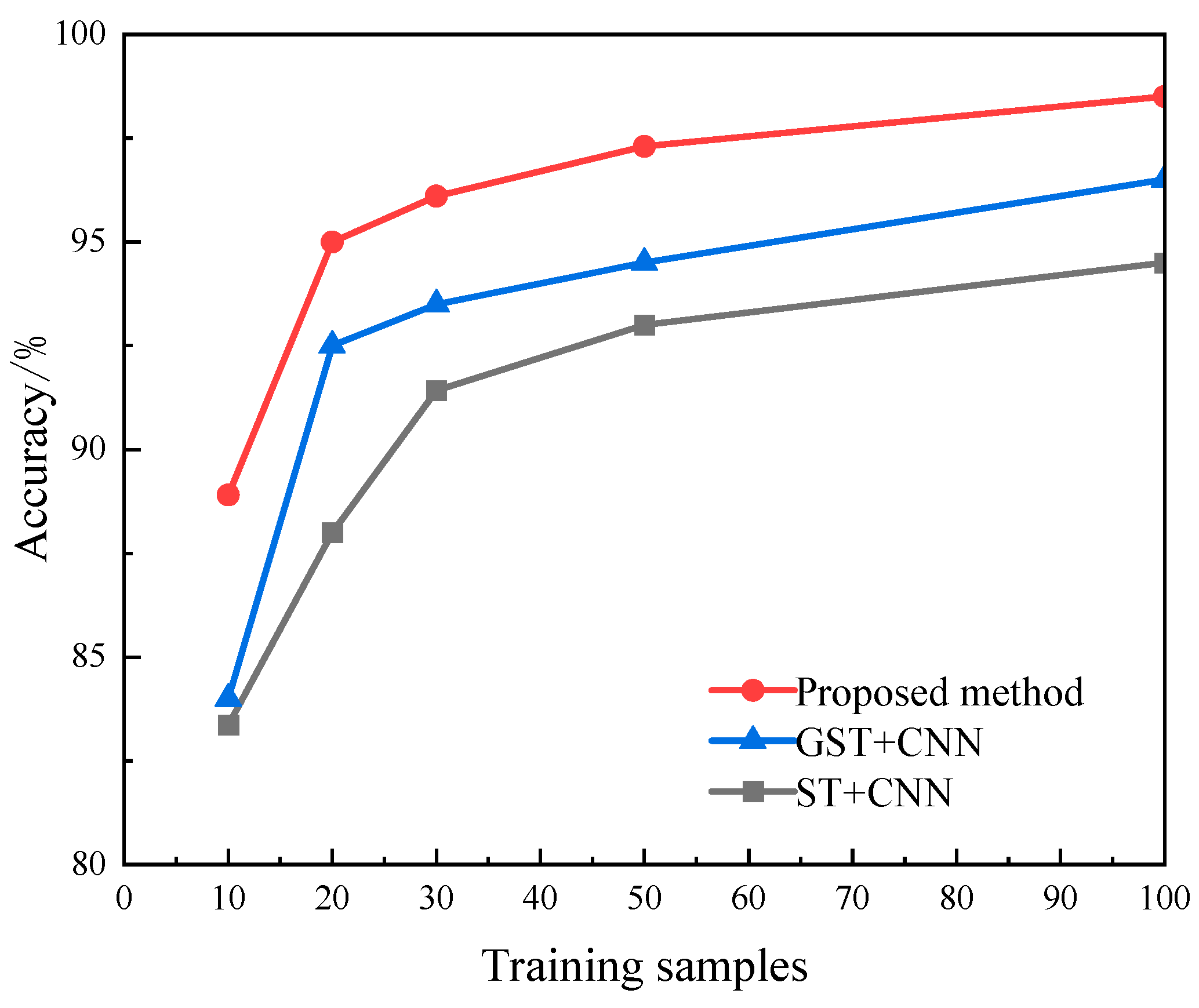
To validate the generalization performance of the proposed model, a multi-scale training set was constructed on the MATLAB platform for comparative experiments. The experimental design is as follows: multiple training sets were constructed, each containing 10 to 100 samples per class (sample sizes set in an arithmetic progression of 10, 20, 30, 50, 100, etc.). Gaussian white noise interference with a 20 dB signal-to-noise ratio was introduced into both the training and testing data. During the testing phase, a test set comprising 22,000 samples (1000 samples per class) was used to evaluate the model’s robustness. The results are shown in Figure 9.

Figure 9. Accuracy with different sizes of training sample.

The results demonstrate that as the training sample size expands, the model’s classification performance exhibits a systematic improvement trend. Notably, this method significantly outperforms the other two classification models across all training scales. When the single-category training sample reaches 50 instances, the model achieves a classification accuracy of 97.3%. Even under under-training conditions with only 10 samples per category, it maintains an accuracy of 88.9%, surpassing the baseline model by 9.5 percentage points. These comparative results fully demonstrate that our approach effectively enhances the model’s feature recognition capability and data efficiency in noisy environments through time-frequency feature optimization and network architecture improvements.

4.5. Actual Data Analysis

To evaluate the algorithm’s performance in real-world scenarios, this study conducted an experimental analysis using power quality disturbance data from the IEEE PES database. This dataset was specifically constructed for power quality disturbance analyses and includes multiple typical disturbance categories. The original sample length comprised 1536 data points. Since the simulation data contained only 1280 data points, this paper used cubic spline interpolation [22] to resample the original 1536 data points to 1280 points. Compared with simple downsampling or end-point copying, interpolation better preserves the original signal morphology, facilitating the retention of high-frequency transient features. Following resampling, all data underwent holistic normalization to eliminate dimensional differences. Four types of typical disturbance signals were extracted from the experiments: 25 voltage swells, 25 voltage dips, 30 harmonics, and 20 transient pulse disturbances. Table 9 presents the experimental results obtained using the model proposed in this paper.

Table 9. Analysis of actual measurement data.

Category	Sample Size	Number of Correctly Classified	Accuracy/%
Voltage surge	25	24	96
Voltage dip	25	25	100
Harmonics	30	29	97
Transient pulses	20	19	98
All	100	97	97

The experimental results indicate that among 25 voltage transient samples, 1 misclassification occurred; among 20 transient pulse samples, 1 misclassification was present; and among 30 harmonic samples, 1 recognition error was identified. The overall recognition accuracy reached 97%.

5. Conclusions

This paper proposes a PQD classification method based on KST and deep neural networks. Through simulation and experimentation, the following conclusions are drawn.

(1)

By improving the control function of the Kaiser window, the adaptability and detection accuracy of the Kaiser window S-transform for power quality disturbance signals are enhanced.

(2)

Under various noise conditions, the model achieves over 98% accuracy in disturbance classification. Furthermore, results from identifying 15 types of composite disturbances generated by the simulation platform demonstrate that the proposed classification model exhibits high accuracy and robust noise immunity for complex power quality disturbances.

(3)

The classification model presented in this paper achieves a comprehensive identification accuracy of 97% for typical disturbances encountered in real-world scenarios. This research holds significant implications for enhancing disturbance identification capabilities in complex electromagnetic environments and preventing relay protection malfunctions caused by power quality issues. The model may provide novel technical support for power quality sensing and early warning in new power systems.

References

- Oubrahim, Z.; Choqueuse, V.; Amirat, Y.; Benbouzid, M.E.H. Disturbances classification based on a model order selection method for power quality monitoring. IEEE Trans. Ind. Electron. 2017, 64, 9421–9432. [Google Scholar] [CrossRef] [Scilit]
- Luo, Y.; Li, K.; Li, Y.; Cai, D.; Zhao, C.; Meng, Q. Three-layer Bayesian network for classification of complex power quality disturbances. IEEE Trans. Ind. Inform. 2017, 14, 3997–4006. [Google Scholar] [CrossRef] [Scilit]
- Valtierra-Rodriguez, M.; Romero-Troncoso, R.D.J.; Osornio-Rios, R.A.; Garcia-Perez, A. Detection and classification of single and combined power quality disturbances using neural networks. IEEE Trans. Ind. Electron. 2013, 61, 2473–2482. [Google Scholar] [CrossRef] [Scilit]
- Achlerkar, P.D.; Samantaray, S.R.; Manikandan, M.S. Variational mode decomposition and decision tree based detection and classification of power quality disturbances in grid-connected distributed generation system. IEEE Trans. Smart Grid 2016, 9, 3122–3132. [Google Scholar] [CrossRef] [Scilit]
- Bai, W.; Zhuang, G.; Zhao, X.; Wei, Z. High-precision intelligent identification of complex power quality disturbances based on improved KST and CNNs. IEEE Access 2024, 12, 86434–86443. [Google Scholar] [CrossRef] [Scilit]
- Cho, S.H.; Jang, G.; Kwon, S.H. Time-frequency analysis of power-quality disturbances via the Gabor–Wigner transform. IEEE Trans. Power Deliv. 2009, 25, 494–499. [Google Scholar]
- Satpathi, K.; Yeap, Y.M.; Ukil, A.; Geddada, N. Short-time Fourier transform based transient analysis of VSC interfaced point-to-point DC system. IEEE Trans. Ind. Electron. 2017, 65, 4080–4091. [Google Scholar] [CrossRef] [Scilit]
- Kawady, T.A.; Elkalashy, N.I.; Ibrahim, A.E.; Taalab, A.-M.I. Arcing fault identification using combined Gabor Transform-neural network for transmission lines. Int. J. Electr. Power Energy Syst. 2014, 61, 248–258. [Google Scholar] [CrossRef] [Scilit]
- Borrás, M.D.; Bravo, J.C.; Montaño, J.C. Disturbance ratio for optimal multi-event classification in power distribution networks. IEEE Trans. Ind. Electron. 2016, 63, 3117–3124. [Google Scholar] [CrossRef] [Scilit]
- Thirumala, K.; Pal, S.; Jain, T.; Umarikar, A.C. A classification method for multiple power quality disturbances using EWT based adaptive filtering and multiclass SVM. Neurocomputing 2019, 334, 265–274. [Google Scholar] [CrossRef] [Scilit]
- Ma, J.; Jiang, J. Analysis and design of modified window shapes for S-transform to improve time–frequency localization. Mech. Syst. Signal Process. 2015, 58, 271–284. [Google Scholar] [CrossRef] [Scilit]
- Wang, Y.; Li, Q.; Zhou, F.; Zhou, Y.; Mu, X. A new method with Hilbert transform and slip-SVD-based noise-suppression algorithm for noisy power quality monitoring. IEEE Trans. Instrum. Meas. 2018, 68, 987–1001. [Google Scholar] [CrossRef] [Scilit]
- Singh, N.; Pradhan, P.M. Efficient discrete S-transform based on optimally concentrated window. IEEE Signal Process. Lett. 2018, 26, 14–18. [Google Scholar] [CrossRef] [Scilit]
- Kumar, R.; Singh, B.; Shahani, D.T.; Chandra, A.; Al-Haddad, K. Recognition of power-quality disturbances using S-transform-based ANN classifier and rule-based decision tree. IEEE Trans. Ind. Appl. 2014, 51, 1249–1258. [Google Scholar] [CrossRef] [Scilit]
- Thirumala, K.; Prasad, M.S.; Jain, T.; Umarikar, A.C. Tunable-Q wavelet transform and dual multiclass SVM for online automatic detection of power quality disturbances. IEEE Trans. Smart Grid 2016, 9, 3018–3028. [Google Scholar] [CrossRef] [Scilit]
- Liang, C.; Teng, Z.; Li, J.; Yao, W.; Hu, S.; Yang, Y.; He, Q. A Kaiser window-based S-transform for time-frequency analysis of power quality signals. IEEE Trans. Ind. Inform. 2021, 18, 965–975. [Google Scholar] [CrossRef] [Scilit]
- Wang, S.; Chen, H. A novel deep learning method for the classification of power quality disturbances using deep convolutional neural network. Appl. Energy 2019, 235, 1126–1140. [Google Scholar] [CrossRef] [Scilit]
- Ren, Z.; Liu, D.; Liu, Y.; Zhang, S.; Hu, H.; Jiang, A. A new parallel PQDs classification method based on an optimized NLM and an improved DRSN-TCN model. Comput. Electr. Eng. 2025, 124, 110326. [Google Scholar] [CrossRef] [Scilit]
- Zaharis, Z.D.; Gravas, I.P.; Yioultsis, T.V.; Lazaridis, P.I.; Glover, I.A.; Skeberis, C.; Xenos, T.D. Exponential log-periodic antenna design using improved particle swarm optimization with velocity mutation. IEEE Trans. Magn. 2017, 53, 1–4. [Google Scholar] [CrossRef] [Scilit]
- IEEE Std 1159-2019 (Revision of IEEE Std 1159-1995); IEEE Recommended Practice for Monitoring Electric Power Quality. IEEE: Piscataway, NJ, USA, 2009; pp. c1–c81.
- Li, J.; Liu, H.; Wang, D.; Bi, T. Classification of power quality disturbance based on S-transform and convolution neural network. Front. Energy Res. 2021, 9, 708131. [Google Scholar] [CrossRef] [Scilit]
- Reda, M.; Onsy, A.; Haikal, A.Y.; Ghanbari, A. A novel reinforcement learning-based multi-operator differential evolution with cubic spline for the path planning problem. Artif. Intell. Rev. 2025, 58, 142. [Google Scholar] [CrossRef] [Scilit]
Disclaimer/Publisher’s Note: The statements, opinions and data contained in all publications are solely those of the individual author(s) and contributor(s) and not of MDPI and/or the editor(s). MDPI and/or the editor(s) disclaim responsibility for any injury to people or property resulting from any ideas, methods, instructions or products referred to in the content. |
© 2026 by the authors. Licensee MDPI, Basel, Switzerland. This article is an open access article distributed under the terms and conditions of the Creative Commons Attribution (CC BY) license.