


Abstract
Smart learning systems are designed to analyze the context, needs, and progress of each student. These are becoming increasingly common, but they present challenges, such as predicting student performance and automatically managing learning activities. In this context, Large Language Models (LLMs) can be useful, as they are capable of understanding word relationships and analyzing their context. They are often associated with chatbots, which are computationally expensive, thereby complicating their integration. Instead, in this work, we propose to leverage the capabilities of LLMs through a semantic graph of activities created from sentence embeddings. This representation is a lightweight and explainable alternative. On the one hand, it requires a lower computational cost. On the other hand, it allows us to observe which activities are most similar directly. On this basis, we propose two problems to validate our proposal. In the first, we use the graph to classify new activities. In the second, we extend this representation with the temporal dimension to formulate a spatio-temporal problem and predict student performance. The results show that the semantic graph not only provides an accurate representation for the organization and classification of activities, but also offers practical advantages and improves explainability.
1. Introduction
Artificial Intelligence (AI) is transforming the educational landscape by enabling more personalized learning experiences through its ability to analyze data, recognize patterns, and support decision-making [1,2]. AI supports a wide range of educational applications on smart learning platforms [3,4], even estimating student performance [5]. Therefore, by integrating it into educational platforms, educators can better understand students’ needs and adapt the learning process. To do this, these platforms need to identify each student and the activities available to them, to characterize students based on their specific characteristics [6]. By characterizing activities, smart learning platforms can characterize students and thus tailor content to them, improving the use of the wide variety of content available in these systems [7]. In addition, it is particularly useful to have a representation that not only describes each activity individually but also enables it to be related to other activities in the system, identifies which ones are most similar, and reuses this information across tasks. However, designing representations that are both computationally efficient and explainable remains a challenge in smart learning systems.
In this work, we propose using embeddings derived from textual activity descriptions as a starting point for constructing a semantic graph of activities. Instead of using embeddings directly as input for each problem, we propose a graph-based representation constructed from a k-nearest neighbors (KNNs) graph and a measure of similarity between activities. This representation offers several advantages for integration into smart learning systems. On the one hand, it is a lightweight alternative to using LLMs via prompting [8,9,10], since embeddings can be computed once and reused. On the other hand, it adds explainability, since the relationship between activities is made explicit in the edges of the graph and can be observed directly through the similarity between nodes. Thus, embeddings are no longer merely numerical representations but also give rise to a reusable relational structure within the system. On this basis, we propose two problems to validate the capabilities of this approach.
In the first, we use the semantic graph to classify new activities, analyzing different methods of semantic space partitioning and showing which one is most suitable for automatically organizing activities. In the second step, we extend this spatial information with the temporal progression of each student’s activities to formulate a spatio-temporal problem. In this context, we seek to predict student performance by considering both an activity’s score and completion time. In both cases, the objective is to verify whether the structure built from embeddings provides a useful, accurate, and explainable representation for relevant tasks within smart learning systems.
This approach differs from the more common ones in AI applied to education, where embeddings are typically used directly as input for each task [11]. In this work, however, they are transformed into a reusable relational structure through a semantic graph of activities. Furthermore, in our work, the graph is constructed directly from the semantic similarity between textual descriptions of activities. This differs from other graph-based approaches, which start from predefined relationships or existing educational structures [12]. Thus, the main novelty of the manuscript lies not only in the use of embeddings or graphs separately, but in their integration as a lightweight, explainable, and reusable representation. In addition, we demonstrate how this can be used both for the classification of activities and for the subsequent formulation of downstream tasks. In our case, this corresponds to a spatio-temporal performance prediction problem.
The main contributions of this work can be summarized as follows:
- A semantic graph representation of learning activities constructed from sentence embeddings, enabling the transformation of semantic similarity into a reusable relational structure.
- An evaluation of graph-based and clustering-based approaches for automatically organizing learning activities within this semantic space.
- A spatio-temporal formulation of student performance prediction, integrating temporal progression with semantic relationships between activities.
- An empirical analysis of different embedding methods, showing how their semantic structure affects graph quality and downstream tasks.
To this end, we first present the theoretical foundations in Section 2. Then, in Section 3, we define the construction of the semantic graph and analyze its use in the classification of new learning activities. Next, in Section 4, we pose the spatio-temporal problem and study the effect of incorporating the semantic structure of the graph into temporal data to predict student performance. Then, in Section 5, we analyze the role of the embedding generation method in the quality of the constructed representation. It also improves explainability by allowing us to visualize how the latent space is structured under different embedding methods. Finally, in Section 6, we present the conclusions from the work carried out.
2. Preliminaries
In this section, we introduce the theoretical foundations necessary to understand the components of the problems and the models that have been used throughout this work.
2.1. Characterization in Smart Learning
A smart learning system is designed to dynamically analyze each student’s context, needs, and progress, with the aim of providing a personalized and adaptive experience [13,14,15]. Typically, the core of a smart learning system consists of one or more algorithms capable of selecting the most appropriate learning activity for each student at a given time, based on their specific characteristics [16]. To do this, both students and activities must be described, typically using a feature vector [17]. This consists of a data structure containing a set of variables that define an entity. In this case, one is used for the activity and another for the student, which is normally updated throughout the learning process. In this way, the system learns about the student through the activities they perform and can analyze which is most appropriate for them at any given time. It is therefore crucial to define these vectors correctly, which can be done in different ways.
These vectors may contain variables representing specific characteristics. For instance, one characteristic could be learning style, which can be defined within different frameworks, such as Kolb’s Learning Style Inventory 4.0 [18] or Gardner’s theory of multiple intelligences [19]. The former establishes nine types of learning styles (i.e., initiating, experiencing, imagining, reflecting, analyzing, thinking, deciding, acting, and balancing). The latter identifies eight types of intelligences, corresponding to eight distinct learning styles (i.e., visual–spatial, linguistic–verbal, logical–mathematical, body–kinesthetic, musical, interpersonal, intrapersonal, naturalistic). These categories denote the possible values a variable can take, corresponding to the learning style in the feature vector.
Additionally, in systems that use deep learning models, it is common to perform this process using embeddings. In the case of text, they are capable of representing semantic meaning and the relationships between words, phrases, or paragraphs. Unlike one-hot encoding, which represents tokens as binary vectors, embeddings assign each element to a continuous vector space, in which similar elements are closer to each other. In the case of Natural Language Processing (NLP), embeddings are learned by models from large amounts of textual data and form the basis of many tasks, as they allow models to work with text in a way that reflects its meaning. In addition, text embeddings provide smart learning systems with tools such as automatic activity classification, enabling faster processing of the large volume of activities that can be entered into these systems.
In addition to representing activities, a smart learning system should include a structure that enables them to be related to one another, identify similar activities, and reuse this information across different tasks within the system. In this sense, a relational representation based on similarity can provide both operational capacity and greater explainability of the system’s behavior.
2.2. Time Series and Spatio-Temporal Problems
Time series are sequences of data recorded over time, often at regular intervals, such as weather data, sensor readings, or records of activities performed by a student. This type of data often involves temporal dependencies, meaning that previous values influence each observation. This makes time series data particularly useful for prediction and for detecting patterns that develop over time.
In deep learning [20], handling time series data requires models that effectively capture temporal dependencies. Traditional methods, such as Auto-Regressive Integrated Moving Average (ARIMA) or Vector Auto-regressive (VAR) [21], often struggle with complex, non-linear patterns. For this reason, models based on Recurrent Neural Networks (RNNs) [22], which process sequential data using a hidden state updated at each time step, have been widely used.
However, standard RNNs have limitations in modeling long-range dependencies due to vanishing and exploding gradients. To address these limitations, more robust recurrent architectures have been proposed, notably the Long Short-Term Memory (LSTM) [23], which incorporates memory cells and gate mechanisms to regulate information flow. Another widely used architecture is the Gated Recurrent Unit (GRU) [24], which simplifies the LSTM architecture by using fewer gates while maintaining the ability to model temporal dependencies effectively with lower computational complexity. Therefore, GRU is a particularly useful alternative when seeking a balance between predictive power and efficiency.
Nevertheless, in certain problems, the temporal dimension is insufficient to describe the data fully. There are scenarios in which each temporal observation is also related to other entities through a spatial or relational structure. In these cases, spatio-temporal problems arise, necessitating the integration of temporal progression with information derived from the existing structure among entities. In our case, this structure is given by the semantic relationships among activities, represented as a graph.
Graphs allow us to model sets of interconnected entities, where nodes represent entities and edges represent relationships between them. To process these types of structures, Graph Neural Networks (GNNs) [25] are used, which extend deep learning to the relational domain by allowing each node to aggregate information from its neighbors. In this way, the learned representations do not depend solely on the characteristics of each node, but also on its context within the graph. Among these architectures, GraphSAGE [26] stands out for learning node representations from aggregating local information, which is particularly suitable for exploiting the connectivity between similar activities.
When temporal models are combined with GNNs, we obtain spatio-temporal architectures capable of simultaneously modeling temporal dynamics and relational structure in data. These architectures, called Spatio-Temporal Graph Neural Networks (STGNNs) [27], allow both dimensions to be integrated into the same model. In this work, this is achieved through an architecture that combines a GRU to model the student’s temporal progression with a 1-hop GraphSAGE aggregation to incorporate the structure of the semantic activity graph. In this way, the problem can be formulated not only as a temporal-sequence problem but also as a spatio-temporal one in which the similarity between activities and the student’s evolution is modeled jointly.
2.3. Communities, Clusters and Activity Classification
In the context of smart learning systems, it is useful to have mechanisms that automatically organize activities based on their descriptions. This is useful both for classifying them and for facilitating their exploration or detecting relationships between them. When embeddings represent activities, this organization can be approached based on the structure of the semantic space. In this case, semantically similar activities tend to be located close together, allowing them to be grouped using various approaches.
One possibility is to construct a graph of activities, where each node represents an activity and the edges represent similarity relationships between nearby activities. Community detection methods, such as Louvain and Leiden [28], can be applied to this type of structure. Both seek partitions of the graph into groups of nodes that are strongly connected to each other and weakly connected to the rest. In this way, they allow the identification of communities of activities that share a high semantic proximity within the constructed relational structure.
A second possibility consists of directly grouping embeddings in a vector space using clustering methods. This work considers k-means, Gaussian Mixture Models (GMMs), and HDBSCAN [29,30]. Although these methods do not operate on a graph, they pursue a similar objective, as they also seek to organize activities into groups based on their proximity in latent space. Therefore, although communities and clusters are obtained in different ways, both can be used later to associate new activities with a semantic category or group.
The main difference between the two approaches is that community methods explicitly exploit the relational structure between activities, while clustering methods work solely with the geometry of the vector space. This makes communities particularly suitable when a structural interpretation of the relationships between activities is desired, while clusters provide a direct partitioning of the latent space without the need to first construct a graph.
In addition to their usefulness for grouping activities, these approaches offer several practical advantages over conventional supervised classification methods, such as Support Vector Machines (SVMs) [31], fine-tuned models on LLMs, or other end-to-end classifiers. First, they allow working with a more scalable representation of the set of activities. Instead of comparing a new activity with all available instances, it can be compared with communities, clusters, or representations associated with them. This reduces the cost of the process as the number of activities grows. Second, these methods do not necessarily depend on a closed set of categories fixed during training. This makes it easier to incorporate new activities and analyze whether they are part of existing groups or give rise to new groupings. This property is especially useful when the activity repository evolves over time and not all categories are fully defined from the beginning.
Another significant advantage is that they allow ambiguous, atypical, or distant activities to be identified more naturally. In these cases, an activity may appear weakly connected to a community, located far from the center of a cluster, or even remain without a clear assignment. This property is especially useful in real-world scenarios, as it allows activities to be flagged for manual review or labeling before being incorporated into the system. In this way, grouping not only serves to automate content organization but also as a support mechanism for the discovery and validation of new activities.
In the context of this work, these properties are particularly relevant because they enable a shift from a representation based solely on embeddings to a structured and reusable organization of activities. Thus, communities and clusters can be used not only to group and classify new activities. They also facilitate exploration of the repository, detect dense or sparse areas of the semantic space, and provide a more explainable basis for their integration into smart learning systems.
2.4. Large Language Models
Large Language Models (LLMs) are models designed to understand and generate human-like text. Built using deep learning techniques, these models are trained on large amounts of textual data from books, websites, and other written sources. Through this training, they learn to predict and generate coherent sequences of words, as well as to understand context and relationships between words. In this way, these models can perform a wide variety of language-based tasks, such as translation, summarization, or question answering [32].
The powerful capabilities of LLMs are made possible by a neural network architecture known as the Transformer [33]. These models revolutionized natural language processing by being able to process entire text sequences efficiently and in parallel, rather than one word at a time. This architecture uses a mechanism called self-attention, which allows the model to weigh the importance of different words within a sentence in relation to each other. As a result, it captures context more efficiently than previous methods, such as RNNs. This architectural strength directly contributes to the adaptability and versatility of LLMs. Because transformers excel at capturing long-range dependencies and context, LLMs can perform complex tasks such as summarizing lengthy documents or generating an embedding that represents the semantic characteristics of a text.
Thus, recent work in time series modeling has begun to incorporate transformer-based architectures [34], which handle long-range dependencies more efficiently and are better suited to large datasets. However, RNNs and LSTMs remain important fundamental models, especially when computational resources are limited or when datasets are relatively small. They offer a good balance between complexity and performance, and their intuitive structure continues to make them valuable tools within the broader landscape of deep learning for time series analysis [35].
2.5. Sentence Embeddings
Sentence embeddings are numerical representations of complete sentences or short paragraphs in a continuous vector space, designed to capture the semantic meaning of the text as a whole. Unlike word embeddings, which represent individual words, sentence embeddings take into account the context and relationships between words in the text, allowing for more accurate comparisons between different sentences. These embeddings are especially useful in tasks such as semantic search or text clustering, where understanding the overall meaning of a sentence is more important than the specific words used.
To generate sentence embeddings, several approaches have been developed, ranging from averaging pre-trained word vectors to using transformer-based models. These models encode the sentence in such a way that similar meanings are assigned to similar vectors, even if the sentences use different words. As a result, sentence embeddings are a powerful tool for processing and comparing natural language at a higher level of abstraction, enabling more accurate and context-sensitive language understanding.
In this work, three approaches have been used to obtain embeddings that encode the descriptions of the activities: CLS tokens, mean pooling of embeddings, and sentence transformers. In the latter case, two different pre-trained models were used: MiniLM and MPNet. The CLS token, short for “classification”, is a special token introduced in transformer-based models to represent a complete input sequence. When a sentence or text is fed into the model, the CLS token is added to the beginning of the sequence. During training, the model learns to use the hidden state corresponding to this token, after passing through the transformer layers, as a summary representation of the entire input. This summary vector captures the contextual information of the entire sentence, due to the self-attention mechanism that allows the CLS token to attend to all other tokens in the input.
An alternative to the CLS token is mean pooling of embeddings, which consists of averaging the embeddings of all tokens in the input sequence to produce a fixed-size vector representation. This method treats the representation of each token equally, combining their contributions to form an embedding representative of the sentence. Mean pooling can be useful because it captures semantic information distributed throughout the sentence rather than relying on a single token. It also avoids potential biases or limitations associated with the CLS token. This token may not always be the most representative feature, especially in models that were not originally designed with this task in mind. In this work, BERT [36] was used to obtain CLS tokens and to perform mean pooling of embeddings.
Sentence Transformers are a specialized class of models designed to produce higher-quality sentence embeddings. Unlike traditional transformer models, such as BERT, which were originally built for token-level tasks, sentence transformers, such as Sentence-BERT (SBERT) [37], modify the architecture to optimize sentence-level representations.
SBERT uses a Siamese architecture, in which two sentences are encoded separately and compared using their embeddings. These models are trained on tasks such as sentence similarity or paraphrase identification, allowing them to learn embeddings that capture detailed semantic relationships. In this work, we have made use of SBERT, using two pre-trained models, one based on MiniLM [38] and the other based on MPNet [39]. In this way, we also seek to examine whether there is a significant difference when varying the models.
Based on these sentence embeddings, activities can be compared with each other in the vector space. This can be done either explicitly using a similarity measure, or implicitly using methods that operate directly on the geometry of the latent space. In this work, the similarity between embeddings is used explicitly to construct the semantic graph of activities. To do this, each activity is connected to those closest to it, thus defining a relational structure on which community detection and spatio-temporal modeling methods are subsequently applied.
On the other hand, some clustering methods, such as k-means, GMMs, or HDBSCAN, work directly on the distribution of embeddings in the vector space. In these cases, proximity between activities remains relevant, but it is not always used through the same explicit similarity formulation as in graph construction. Instead, these methods exploit the geometry of the latent space to cluster activities that are close to each other.
In the case of graph construction, the similarity between two embeddings can be expressed using cosine similarity, which measures the angular proximity between two vectors in vector space. This metric takes the value 1 when both vectors point in the same direction, 0 when they are orthogonal, and −1 when they point in opposite directions. Cosine similarity is defined as:
where A and B are the sentence embeddings, · is the scalar product, and is the magnitude.
Based on these foundations, the following sections present the experimental evaluation of the proposed semantic graph representation.
3. Semantic Graph for Activity Classification
This section introduces the first problem addressed in this work, which focuses on constructing a semantic graph of activities and using it to classify new activities. To this end, we present the dataset used, the process of building the graph from embeddings, the methods evaluated, and the experimental results obtained.
3.1. Dataset for Activity Classification
The EduQG [40] dataset was used for the activity classification problem. This is an educational dataset containing multiple-choice questions, their correct answers, and excerpts from teaching materials used as sources. The dataset was constructed by education experts, ensuring the pedagogical quality of the questions, and is divided into train and test partitions.
For this problem, the field question_text was used for each question, which corresponds to the question statement. Each instance in the dataset also includes a topic identifier, called bname. This indicates the book or topic unit from which the question comes, for example, biology or u.s._history. As these identifiers correspond to specific topics, they have been grouped into academic subjects to approach classification from a knowledge area perspective. This perspective is closer to the reality of smart learning systems.
This grouping was not done with the aim of reducing the number of classes, but rather to better align the task with the objective of the work. The original bname identifiers correspond to specific books or thematic units, whereas in many smart learning scenarios it is more useful to distinguish between broader areas of knowledge. Furthermore, several of the original labels share thematic affinity and semantic proximity. Therefore, their aggregation allows us to analyze whether the relational structure induced by the embeddings and the graph is capable of identifying patterns at the level of academic subjects, and not just differences between specific materials. From this perspective, reformulating the problem across four broad subject areas allows us to evaluate the method’s performance on a task more aligned with real-world educational contexts.
The grouping of the different identifiers into academic subjects has been as follows:
- Biological And Health Sciences
- –
- biology
- –
- microbiology
- –
- anatomy_and_physiology
- History And Government
- –
- u.s._history
- –
- american_government
- Social And Behavioral Sciences
- –
- psychology
- –
- introduction_to_sociology
- Business And Accounting
- –
- business_ethics
- –
- principles_of_accounting,_volume_1:_financial_accounting
- –
- principles_of_accounting,_volume_2:_managerial_accounting
- –
- business_law_i_essentials
- –
- introduction_to_intellectual_property
After applying this grouping process, the resulting class distribution shows some imbalance. In the train partition, the dataset consists of 1373 instances belonging to Biological And Health Sciences, 525 toBusiness And Accounting, 458 to Social And Behavioral Sciences, and 359 to History And Government.
Similarly, in the test partition, there are 302 instances of Biological And Health Sciences, 174 of Social And Behavioral Sciences, 105 of History And Government, and 88 of Business And Accounting. This distribution reflects the heterogeneity of the original dataset and highlights the need to use appropriate metrics and evaluation strategies for multi-class classification scenarios with unbalanced classes.
From the question_text field, representations of the activities have been generated using sentence embeddings. These representations allow each question to be projected onto a continuous vector space in which texts with similar semantic meaning tend to be located close to each other.
To analyze the impact of the representation method, four variants of the dataset were considered based on the technique used to obtain the embeddings: CLS, mean pooling, MiniLM, and MPNet. In this way, all instances share the same text and the same labels. They vary only in the way the activity is encoded in the vector space, which allows us to evaluate the influence of the type of embedding on the performance of the different methods.
3.2. Graph Construction
Based on the set of activities represented by embeddings, a KNN graph was constructed from their proximity in the semantic space. First, the embeddings were normalized using the L2 norm [41], so that the comparison between activities is performed in terms of angular similarity. Next, for each activity, its k nearest neighbors were identified using cosine distance, excluding the node itself from the search.
The initial graph is defined as a directed KNN structure, in which each node is connected to its k nearest neighbors. The edge weights are calculated based on the measure defined in Equation (1), where A and B are the embeddings corresponding to the learning activities. In this way, the activities closest in the semantic space receive higher weights. Subsequently, this directed structure is transformed into an undirected weighted graph through a symmetrization process. Specifically, an undirected edge is included between two nodes whenever at least one of them appears among the other’s k-nearest neighbors. When the relationship exists in both directions, the final weight of the edge is defined as the maximum corresponding similarity value.
The graph construction parameters are selected from the training data through a hyperparameter search using validation. Specifically, the value of k is adjusted in conjunction with the resolution parameter of the community detection algorithm using a stratified train-validation split. The final configuration is selected based on the highest Macro F1 score in the validation set. Likewise, the effect of different values of k was analyzed. This analysis showed that very low values, such as , can result in more fragmented graphs. However, for intermediate and medium-high values in the analyzed range between and , predictive performance remains stable.
This construction transforms the continuous embedding space into a discrete and reusable structure, suitable for clustering, classification, and subsequent modeling tasks. First, it allows the activities most similar to a given activity to be directly retrieved through its edges. Second, it provides a structured basis on which community detection methods, such as Louvain or Leiden, can be applied, while maintaining explicit local connectivity between activities. This representation offers practical scaling advantages, as a new activity can be compared to communities, prototypes, or areas of the graph, rather than requiring exhaustive comparison with all available instances.
In addition, this structure also facilitates the detection of ambiguous or atypical activities. When an activity is weakly connected, has few similarities with its neighbors, or is located in low-density regions of the graph, it can be identified as a case that should be reviewed manually before its final incorporation into the system. Finally, the graph adds explainability, since the relationships between activities are defined by observable similarities and by their position within an explicit relational structure. This representation also improves explainability, since the relationships between activities are explicitly encoded as edges in the graph. As a result, the influence of previous activities can be interpreted through their semantic neighbors and the similarity weights connecting them. This provides a transparent mechanism to understand how activities are related within the system.
3.3. Graph Partitioning Methods
To address this problem, different methods capable of automatically organizing activities based on their semantic representation were evaluated. First, Louvain and Leiden were considered as two community detection methods applied to the weighted graph derived from the local neighborhoods between activities. Both allow the identification of groups of nodes that are strongly connected to each other and weakly connected to the rest, explicitly exploiting the relational structure of the semantic graph. Although the two methods pursue the same objective, Leiden tends to show more robust behavior by generating better-connected partitions.
In addition, several clustering methods were included as a reference: k-means, Gaussian Mixture Models (GMM), and HDBSCAN. Unlike Louvain and Leiden, these methods do not operate on the explicit structure of the graph or on the edges derived from the similarity between activities. Instead, they operate directly on the distribution of embeddings in the latent space. This allows us to compare whether the construction of the semantic graph provides a real advantage over approaches based solely on the geometry of the vector space.
3.4. Metrics for Activity Classification
We used Accuracy, Balanced Accuracy, Macro Precision, and Macro F1 to compare the performance of the methods evaluated on the activity classification problem. Accuracy measures the total proportion of correctly classified instances. By contrast, macro metrics allow for a more balanced evaluation of the model’s behavior across classes, which is particularly relevant in unbalanced scenarios such as the present one. Macro Recall was not included as a separate metric, since in this single-label multi-class classification setting it is equivalent to Balanced Accuracy.
The definition of the metrics is as follows:
where , , , and represent, respectively, the number of true positives, false positives, true negatives, and false negatives for class c. In the case of Accuracy, , , , and correspond to the global counts for all classes, and K represents the total number of classes.
3.5. Training for Activity Classification
For the evaluation, the original train and test partitions of the EduQG dataset were maintained. Hyperparameter selection was performed only on the training partition, generating a stratified train/validation split in each run, with 20% of the data reserved for validation. On this split, the different methods were compared by optimizing Macro F1.
Once the best configuration was identified in validation, each method was adjusted again using the complete training partition and evaluated on the test partition. This process was repeated 10 times, varying the seed in each run, in order to analyze the stability of the results against the randomness of the process. The final result reported for each combination of method and embedding corresponds to the aggregation of the metrics obtained in the test throughout the 10 runs.
3.6. Comparison for Activity Classification
Table 1 shows the results obtained by the different methods when used together with different types of embeddings in the activity classification problem. When comparing these, it can be seen that the best results are obtained by Leiden when combined with MPNet embeddings. Specifically, this configuration obtains the best results in Accuracy, Balanced Accuracy, Macro Precision, and Macro F1, reaching values of 87.23% ± 0.94%, 84.28% ± 1.68%, 86.80% ± 1.01%, and 84.71% ± 1.49%, respectively.
Table 1.
Comparison of the results obtained by the methods in different datasets in the activity classification problem. The best result for each metric is shown in bold.
These results suggest that exploiting the relational structure induced by embeddings provides advantages over approaches that rely solely on the geometry of the embedding space. In particular, the combination of Leiden and MPNet embeddings achieves the best overall performance, reaching an Accuracy of 87.23%, a Balanced Accuracy of 84.28% and a Macro F1 score of 84.71%. In addition, a paired permutation test was performed to assess whether the improvement achieved by Leiden with MPNet embeddings over the other models was consistent. Statistically significant improvements were observed for the Leiden with MPNet version in the comparisons conducted.
If we observe the behavior of the different embeddings, we can see that the best results are consistently concentrated in MiniLM and MPNet, regardless of the method used. This indicates that embeddings generated with sentence transformers provide a better semantic space for organizing activities. This can be observed both in clustering methods and in community detection methods. In contrast, CLS and mean pooling perform significantly worse in all methods, suggesting that the semantic structure they create is less useful for this problem.
Among the methods evaluated, Leiden and Louvain show particularly competitive performance when applied to graphs constructed from MiniLM and MPNet. In the case of MPNet, Leiden outperforms Louvain in all four metrics considered, while in MiniLM, both methods produce very similar results. These results indicate that the semantic graph provides an effective representation for automatically organizing learning activities, and that Leiden is particularly effective at exploiting this structure.
On the other hand, k-means and GMM also obtain competitive results when combined with MiniLM and MPNet, although they generally remain below the best results obtained with graph-based methods. This suggests that the geometry of the latent space already contains useful information for organizing activities, but that this information can be better exploited when transformed into a graph. In contrast, HDBSCAN shows clearly inferior performance in all cases, especially with CLS and mean pooling, indicating that it is not suitable for this problem. This behavior may be related to the relatively uniform density of the embedding space, which limits the ability of density-based methods to identify stable clusters.
To complement the above comparison, we have analyzed in greater detail the configuration that achieved the best results, which corresponds to Leiden with MPNet. Table 2 shows the precision, recall, and F1 score for each class, while Figure 1 presents the confusion matrix for the best run of this configuration. This analysis provides a better understanding of the model’s performance across different classes and helps identify the main error patterns.
Table 2.
Per-class metrics obtained using Leiden with MPNet on the activity classification problem.
Figure 1.
Confusion matrix for the best run of Leiden with MPNet on the activity classification problem.
Table 2 shows the results for each class. From these, we can see that Biological And Health Sciences is the category with the best performance, achieving the highest F1 score and nearly perfect recall. Business And Accounting also performs well and has balanced metrics. In contrast, History And Government achieves a relatively high recall but lower precision. This suggests that the model tends to overpredict this class in some cases. The most challenging category is Social And Behavioral Sciences, which achieves the highest precision but a considerably lower recall. This indicates that many of its actual instances are classified as other classes.
This pattern can also be observed in Figure 1, which shows the model’s confusion matrix. In this matrix, it can be observed that a significant number of instances of Social And Behavioral Sciences are classified as Biological And Health Sciences or as History And Government. In contrast, Biological And Health Sciences appears to be classified better than the other categories. These results show that there are differences in prediction performance across classes. However, despite these differences, in the class with the highest number of errors, the model achieves an F1 score of 79.29%. Therefore, even in the worst-case scenario, the classification performance remains strong.
Thus, these results show that semantic graphs allow activities to be classified with high accuracy. In this way, their use combines all the advantages associated with graph-based representations with high predictive power. At the same time, the results also show the relevance of the embedding used, as can be seen from its impact on the results obtained by Louvain and Leiden.
3.7. Performance Comparison
The previous comparison demonstrates how the use of graphs with Leiden can outperform clustering methods and achieve effective classification. This approach provides an effective classification method while leveraging the advantages of the graph structure. However, to complement the previous evaluation and compare it with other models focused solely on classification, Leiden was compared with supervised classification methods. Specifically, it was compared with SVM, Random Forest, Residual MLP and KNN. Furthermore, all methods use the same embeddings obtained with MPNet as input. Thus, the observed differences can be attributed to the classification method and not to changes in the semantic representation. In addition, a hyperparameter search was conducted to identify the optimal settings.
However, this comparison aims to go beyond simply comparing the predictive performance of the models, as our proposal does not focus solely on that. For this reason, we have designed a simulation of a real production environment. In this simulation, all models are initially trained on the original EduQG dataset. Next, a loop is performed, in which 1000 additional learning activities are predicted so they can be classified. Then, the model is retrained, but using their actual labels rather than the predicted ones. This simulates a cycle of prediction and model retraining in which the smart learning system accumulates data.
The experiment starts with the original EduQG training dataset and progressively expands it with new synthetically generated activities. To do this, each original activity was automatically reformulated using a sequence-to-sequence generative model, specifically Flan-T5 [42]. Generation was approached as a controlled paraphrasing task, using various prompts designed to produce semantically equivalent reformulations while preserving the question’s meaning, its intended response, and its interrogative form. In particular, prompts were used to obtain alternative versions of the same activity through changes in wording, reformulation for students, lexical variation, and rephrasing while maintaining the same semantic constraints. Additionally, different sampling-based generation configurations were combined, modifying parameters such as temperature, top-p, and repetition penalty, with the aim of increasing the linguistic diversity of the generated variants.
Based on this procedure, a set of synthetic variants was constructed for each original activity. In this incremental experiment, the dataset was progressively expanded up to a maximum of twenty times the original size of the training set. New activities were incorporated in a nested manner. That is, in each round, a new reformulation was added per activity before moving on to the next. This allows us to simulate a gradual influx of new content while preserving the structure of the original dataset. Starting from the base dataset, the system incorporates successive blocks of 1000 new activities. It then retrains on all supervised classification models, or updates the model with all available data in the case of Leiden. The process is then repeated until the number of iterations specified in the experiment is completed. However, it is important to note that the expansion was not performed on the test data. Therefore, the accuracy and Macro F1 scores obtained in each iteration are based on the original test set.
In the case of Leiden, HNSW [43] was used to approximate the k-nearest neighbors graph. This method trades some accuracy in identifying the nearest neighbors for faster performance and the ability to dynamically insert new data into the index. In the initial iteration, the model is trained in the usual way. Thus, the graph is constructed over the training set, and Leiden is applied to detect communities. From these communities, both the distribution of labels per community and the cluster centroids in the embedding space are obtained. However, in subsequent iterations, the complete graph is not reconstructed, nor is the community detection algorithm re-run on all nodes. Instead, the embeddings already in use are stored in an HNSW index, and each new activity is inserted by querying its nearest neighbors among the existing nodes. The new activity is assigned to the most frequent cluster among the retrieved neighbors, and when no reliable assignment based on proximity exists, the nearest cluster centroid is used as a fallback. Once the new node is assigned, the label counts of its cluster and the corresponding centroid are incrementally updated. The centroid is recalculated based on the cumulative sum of normalized embeddings and the updated cluster size. In this way, the method preserves the initial community structure and adapts its internal representation through successive insertions, avoiding the cost of recomputing the graph and re-running Leiden in each iteration.
This is particularly relevant for interpreting computational cost. This incremental variant of Leiden shifts the computational effort to the update phase. Subsequent prediction is performed by assigning nodes to the nearest centroid and consulting the label distribution of the corresponding cluster. This keeps the inference cost very low even as the total number of activities increases. Therefore, the time complexity of the method depends not only on the use of Leiden as a community detection algorithm, but also on this incremental strategy based on the insertion of new nodes and the updating of centroids. This demonstrates the flexibility provided by the graph architecture.
The accuracy and Macro F1 results are shown in Figure 2 and Figure 3. In terms of predictive performance, SVM achieves the best average results throughout the incremental process. However, Leiden maintains competitive and stable performance, with average accuracy and Macro F1 scores very close to those obtained by the best supervised classifiers and superior to those of Residual MLP. Furthermore, Leiden remains stable throughout the iterations. In contrast, when observing KNN, its performance declines significantly as the size of the training set increases. These results indicate that the graph structure allows for the preservation of high predictive capability even in an incremental context. Although this is a limited result, given the use of synthetic data, it does demonstrate Leiden’s ability to maintain its predictive performance with the proposed method.
Figure 2.
Evolution of the accuracy in the incremental simulation for the various methods evaluated.
Figure 3.
Evolution of the Macro F1 in the incremental simulation for the various methods evaluated.
Figure 4 and Figure 5 show the temporal evolution of the different methods. These figures display the training time and prediction time for each iteration, respectively. Additionally, Figure 6 shows the total accumulated time across the different iterations. When comparing these, it can be seen that Leiden performs particularly well. Its training time remains low across all iterations, and its prediction time is practically constant and very low. In contrast, SVM and Random Forest show a very significant increase in training time as the dataset grows. In the case of SVM, moreover, prediction time increases the most, becoming particularly slow compared to the other alternatives. In the case of Residual MLP, it can be seen that while the training time is more moderate, it still significantly exceeds Leiden’s. Furthermore, when comparing accuracy and macro F1, Residual MLP obtains worse results, so it offers no advantage. It is important to note that the more abrupt changes in Residual MLP’s training time are due to the fact that an early stop has been set during its training to try to optimize the training time.
Figure 4.
Evolution of training time per iteration in the incremental simulation for the various methods evaluated. The results from KNN and Leiden overlap, as they obtain similar values.
Figure 5.
Evolution of prediction time per iteration in the incremental simulation for the various methods evaluated. The results from Residual MLP and Leiden overlap, as they obtain similar values.
Figure 6.
Evolution of total accumulated time, taking into account training and prediction in the incremental simulation.
In the case of KNN, it has a very low training cost. However, its inference time increases progressively with the number of activities, which limits its applicability in scenarios where prediction latency is a critical factor and the amount of data is increasing. Even so, KNN and Leiden remain the two methods with the lowest total time in Figure 6. Therefore, a specific comparison of the two has been conducted to better evaluate them.
A more detailed comparison between KNN and Leiden can be seen in Figure 7. In KNN, the prediction time and, consequently, the total time per iteration, increase steadily as new activities are added. In contrast, Leiden maintains a virtually constant prediction time. As a result, it achieves a low and stable total time per iteration, concentrating the computational cost primarily on updating the graph structure during training. This is particularly relevant in production contexts where predictions must be made frequently on a growing volume of activities.
Figure 7.
Comparison between KNN and Leiden in terms of training time, prediction time, and total time per iteration in the incremental simulation.
Overall, the results of this simulation allow us to draw two conclusions. First, a comparison with supervised classifiers trained on the same embeddings shows that Leiden delivers competitive and stable results. On the other hand, performance metrics confirm that this is a computationally lightweight approach, especially when considering the balance between training, inference, and progressive scaling of the system. In this regard, Leiden offers a favorable performance-to-cost ratio, which reinforces its potential in smart learning systems.
4. Spatio-Temporal Modeling of Student Performance
This section presents the second problem used to validate our approach. In this case, the spatial information obtained from the semantic graph is combined with the student’s temporal progression to formulate a spatio-temporal problem. In our case, the objective is to predict the score obtained in an activity and the time taken to complete it. To this end, both the student’s historical information and the semantic relationships between activities have been incorporated.
4.1. Dataset for Student Performance Prediction
For this problem, we used a proprietary dataset obtained from a smart learning system. It captures the progression of scores and the time, in seconds, taken by different students to complete the activities. The dataset collects the interaction of 79 students with 582 different learning activities, resulting in 18,989 completed attempts. Therefore, each student completed about 240 attempts on average. Figure 8 and Figure 9 show the distributions of the variables Score and Seconds, respectively. Five new datasets have been generated from this dataset.
Figure 8.
Visualization of the distribution of the variable Score.
Figure 9.
Visualization of the distribution of the variable Seconds.
The first of these datasets, called No similarity, consists of time series constructed independently for each student based on their chronological activity history. To generate these sequences, interactions were sorted by start date, and sliding windows of 11 time steps were created. Of these, the first 10 correspond to the input provided to the model, and the last one corresponds to the values to be predicted. Thus, each input time step represents the score obtained on an activity and the time the student took to complete it, while the target corresponds to the next activity in the sequence. In this way, each sample is constructed solely from information available prior to the target activity, avoiding the use of future interactions regarding the student’s progress.
In addition, four more versions of the dataset were used: CLS, mean pooling, MiniLM, and MPNet. These versions incorporate a spatial dimension derived from the semantic graph, including three variables obtained from the relationship between the activity of that timestep and the target activity in each timestep. The first of these variables is similarity, which corresponds to the weight of the graph edge between the two activities. The second represents the maximum similarity observed up to that point in the sequence. The third corresponds to the average of the three highest similarities observed up to that timestep. In this way, the student’s temporal sequence is enhanced with structural information from the semantic graph.
Thus, the problem can be formulated by integrating two complementary dimensions. The first is a temporal dimension, defined by the student’s progression through the activity sequence. The second is a spatial dimension, determined by the relative position of activities within the semantic graph. By combining these two perspectives, the task can be modeled as a spatio-temporal problem in which the semantic relationships between activities contribute to improving performance prediction. Moreover, the use of similarity across graph edges enhances explainability, as it makes it possible to trace the relevance of different activities through their connections in the graph.
4.2. Models for Student Performance Prediction
This combination of spatial structure and temporal progression can be approached in two ways. The first consists of extracting spatial information from the graph beforehand and then adding it as variables within a conventional time series. The second consists of directly integrating the graph structure into the model. In this case, the spatial and temporal dimensions are processed together. This work considers both perspectives to analyze the added value of explicitly modeling the structure of the semantic graph.
In the first approach, BiLSTM and Transformer are used on different versions of the sequential dataset. Although these models are temporal architectures, in the enriched versions they do not operate solely on the original sequence, but also on the three spatial variables derived from the semantic graph. In this way, spatial information is integrated into the input prior to training. Thus, the problem is formulated as a two-phase spatio-temporal problem: first, the relational information is extracted manually and then entered into a standard temporal model.
The first of these models uses a Bidirectional LSTM (BiLSTM) [44]. These extend the capabilities of standard LSTMs by processing the input sequence both forward and backward. This means that, at each timestep, the model has access not only to past information, but also to future context within the sequence. In several tasks, BiLSTMs have been shown to outperform unidirectional models because they capture broader contextual information. This dual perspective improves the model’s ability to understand dependencies that might be overlooked when looking at data in only one direction.
The second model is based on the Transformer architecture. In time series problems, transformers have demonstrated strong performance by effectively modeling long-range dependencies and capturing complex temporal patterns. Unlike traditional sequential models, transformers can simultaneously process the entire time series input, allowing them to learn relationships between distant timesteps without the limitations of step-by-step processing. The version used in this work makes use of a single Transformer layer adapted to the problem and does not incorporate the positional embeddings present in the original implementation.
The second approach corresponds to the STGNN model. In this case, the spatial structure is not introduced through previously calculated variables, but directly through the connections of the semantic graph. The model combines a 1-hop GraphSAGE aggregation on the activity graph with a GRU that models the temporal evolution of the sequence. For each activity in the sequence, the representation obtained from its neighbors in the graph is concatenated with the numerical variables of the corresponding timestep. This enriched sequence is then further processed by the GRU layer. In this way, the spatial and temporal dimensions are integrated within the same architecture, allowing the connectivity between activities and student progression to be modeled jointly.
4.3. Metrics for Student Performance Prediction
To compare the different models, we used Mean Absolute Error (MAE), Root Mean Square Error (RMSE), and Symmetric Mean Absolute Percentage Error (SMAPE). MAE and RMSE are two of the most commonly used metrics for comparing the accuracy of models in time series and spatio-temporal problems. In addition, SMAPE was used. This is a modified version of Mean Absolute Percentage Error (MAPE) that eliminates MAPE’s limitation when values can be 0. The definition of the metrics is:
where N is the number of cases, is the actual value, and is the prediction.
4.4. Training for Student Performance Prediction
For training, the dataset was divided into training, validation, and test sets using a fixed split of 80%, 10%, and 10%, respectively, at the student level. Thus, all sequences generated from a single student’s history were assigned to a single subset. This decision prevents closely related time windows from the same student from appearing simultaneously in training and evaluation, which would artificially reduce the difficulty of the prediction task. This partition remained constant across runs, so that any observed differences in results were due to training randomness and not to changes in the composition of the subsets. In all models, an early stop based on validation loss was used, with a patience of 100 epochs, and RAdam [45] as the optimizer. Table 3 summarizes the hyperparameters used during training.
Table 3.
Hyperparameters used during model training.
In the case of BiLSTM and Transformer, training was carried out on different versions of the sequential dataset. The No similarity version contains only the original temporal variables, while the embedding-based versions also incorporate spatial variables derived from the graph. Therefore, although the architectures used are temporal, in these configurations training is already performed on a sequence with previously extracted relational information.
For STGNN, the data explicitly incorporates both the temporal sequence and the structure of the semantic graph. To do this, the model uses the nodes, edges, and weights of the previously constructed graph. It then generates a representation of the activity at each timestep based on its neighbors using a 1-hop GraphSAGE aggregation. This representation is concatenated with the numerical variables of the sequence and processed by a GRU, allowing the temporal information and spatial structure of the graph to be integrated into a single architecture.
It should be noted that this strategy does not involve a global temporal partition based on dates, but rather a student-level partition of sequences that are internally ordered chronologically. Therefore, the evaluation mainly measures the ability to generalize to unseen students while keeping the set of activities fixed. In this sense, the same activity may appear in different subsets associated with different students.
Each configuration was trained 10 times, varying the seed in each run, in order to analyze the stability of performance in the face of the randomness of the training process. The final result reported for each combination of model and dataset corresponds to the aggregation of the metrics obtained in the test partition throughout the 10 runs.
4.5. Comparison for Student Performance Prediction
Table 4 summarizes the results obtained by the different models in the task of predicting student performance, considering both target variables together. Each configuration was trained 10 times with varying seed values in order to analyze the stability of performance given the randomness of the training process. The reported values correspond to the aggregation of the metrics obtained on the test set across these runs.
Table 4.
Comparison of the average results obtained by the models across different datasets, taking both target variables into account. The best result for each metric is shown in bold.
Table 4 shows that incorporating semantic information across activities generally improves results compared to the No similarity version. This trend is observed in both the temporal models and the spatio-temporal model. Thus, it is shown that spatial variables derived from the graph provide useful information for predicting the outcome of an activity based on the student’s prior progress. In the temporal models, both BiLSTM and Transformer improve their results when incorporating information derived from embeddings. In the case of BiLSTM, the best configuration corresponds to MiniLM, which achieves the best RMSE within this model. In the case of Transformer, the best performance is also achieved with MiniLM, with consistent improvements over No similarity across all three metrics. However, the best overall result is achieved with STGNN and MiniLM, which obtains the lowest MAE and the lowest SMAPE in the table, in addition to a competitive RMSE.
These results suggest that combining the semantic structure of the graph with the student’s temporal progression allows for the construction of a more informative representation for prediction. In addition, a paired permutation test was performed to assess whether the improvement achieved by STGNN with MiniLM embeddings over the other models was consistent. Statistically significant improvements were observed for the STGNN with MiniLM version in the comparisons conducted.
Although these results provide an overview of the performance of the models, this problem involves predicting two different variables: score and time. For this reason, Table 5 and Table 6 have been added. These tables present the results broken down by each variable. This analysis allows us to verify whether the incorporation of semantic information derived from embeddings affects both variables similarly or whether its impact depends on the prediction target.
Table 5.
Comparison of the metrics obtained by the models across different datasets when predicting the score variable. The best result for each metric is shown in bold.
Table 6.
Comparison of the metrics obtained by the models across different datasets when predicting the time variable. The best result for each metric is shown in bold.
When analyzing both target variables separately, it becomes clear that the effect of embeddings is not uniform. In Table 5, the differences between configurations are very small. In particular, the results for the Transformer vary only slightly between the No similarity version and the versions that incorporate embeddings. In STGNN, the metrics are practically identical for all semantic representations considered. Even in BiLSTM, where small variations do appear, the improvements are limited. Taken together, these results indicate that the prediction of score is barely affected by the incorporation of semantic information.
In contrast, Table 6 shows a distinctly different pattern. In this case, the incorporation of embeddings yields notable improvements across all models, and these are particularly evident in the Transformer. The difference between the No similarity version and the configurations with embeddings is pronounced across all three metrics. This indicates that semantic information across activities is particularly relevant for predicting the time spent by the student. BiLSTM also improves consistently when embeddings are incorporated, although to a lesser extent. Once again, the best overall result corresponds to STGNN with MiniLM, which achieves the lowest values for MAE, RMSE, and SMAPE. Therefore, the broken-down results show that the gain observed in the overall comparison comes mainly from the improvement in the prediction of time, whereas for score the effect of embeddings is much smaller.
Taken together, these results indicate that the semantic information derived from the graph does not contribute equally to the two target variables. While its effect on score is limited, its contribution to the prediction of time is clear and consistent. This reinforces the idea that semantic relationships between activities capture information that is particularly useful for modeling the time effort associated with task completion.
5. Embeddings Analysis
Although the different results obtained show the capacity of MiniLM and MPNet to obtain better embeddings, to improve the explainability of our approach, we have analyzed the embeddings obtained from the EduQG dataset. This analysis allows us to better explain our approach and understand where the differences observed between embeddings arise.
5.1. Embeddings and Communities Visualization
To this end, CLS and MPNet embeddings are visualized using UMAP [46] projections in two and three dimensions. These visualizations serve as an analysis tool to observe how the semantic space induced by each method is organized. They also help assess how this organization can influence the subsequent construction of the graph and the detection of communities. In all the visualizations in this section, each point represents an activity in the dataset, and the color indicates its academic subject. The axes correspond to the UMAP components and thus reflect a low-dimensional projection of the original semantic space. In this projection, the proximity between points indicates greater semantic similarity between activities.
Figure 10 and Figure 11 show that CLS embeddings present a strong overlap between classes, both in two-dimensional and three-dimensional projections. The different activities appear to be highly mixed, without a clearly separated distribution. This suggests that, although these embeddings may contain useful information, that information is not organized in a particularly favorable way for tasks that depend on local semantic proximity or a well-defined relational structure. In contrast, Figure 12 and Figure 13 show greater separation between classes in MPNet embeddings, where samples tend to cluster more compactly according to academic subject.
Figure 10.
2D visualization using UMAP of the CLS embeddings for the activities in the EduQG dataset. Each point represents an activity, and the color indicates its academic subject. There is considerable overlap between classes and limited separation between regions of the space. This suggests a less well-defined semantic organization for this type of representation.
Figure 11.
3D visualization of CLS embeddings using UMAP. The spatial distribution confirms the pattern observed in two dimensions. Activities from different subjects appear heavily mixed and do not form clearly distinct clusters. This makes it difficult to identify a compact semantic structure.
Figure 12.
2D visualization using UMAP of the MPNet embeddings for the activities in the EduQG dataset. Each point represents an activity, and the color indicates its academic subject. In this case, a clearer separation between various classes is observed, along with a tendency to form more compact clusters. This suggests a more coherent semantic organization than that observed with CLS.
Figure 13.
3D visualization of MPNet embeddings using UMAP. This visualization reinforces the greater separability between classes observed in 2D and reveals more compact and better structured regions. This facilitates subsequent tasks based on semantic proximity.
This difference can be explained by the training objectives of each type of embedding. Sentence transformer models are trained to produce sentence-level representations in which semantically similar texts tend to be located close to each other. In contrast, CLS embeddings obtained from BERT [36] are not specifically optimized to directly preserve this type of global semantic structure in the latent space. As a result, the space generated by MPNet favors a more coherent organization for tasks based on proximity and clustering.
This difference can also be observed when analyzing the communities detected on the graph constructed from both types of embeddings. Figure 14 and Figure 15 show the same 2D UMAP projections as above, but adding the communities obtained using Leiden. In addition, visualizations created with Leiden display the graph connections and the centroids of the detected communities. The larger and numbered nodes represent these communities, while the edges reflect proximity relationships between activities in the semantic graph.
Figure 14.
2D projection using UMAP of the CLS embeddings together with the communities detected by Leiden in the semantic graph. The colored points represent activities based on their academic subject. The edges show proximity relationships in the graph. The larger and numbered nodes correspond to the community centroids, with each number representing the community ID. A more mixed distribution is observed, with communities that do not align clearly with homogeneous semantic regions.
Figure 15.
2D projection using UMAP of the MPNet embeddings together with the communities detected by Leiden in the semantic graph. The colored points represent activities according to their academic subject. The edges show proximity relationships in the graph. The larger and numbered nodes correspond to the community centroids, with each number representing the community ID. Compared to CLS, the communities show a clearer correspondence with compact regions of the semantic space. This facilitates a more coherent relational structure.
In the case of CLS, communities appear in a much more mixed distribution, making it difficult for the graph structure to reflect clean and consistent semantic groupings. In contrast, in MPNet, communities correspond better to compact regions of space. This helps to understand why this type of embedding produces better results in graph construction and in subsequent methods that depend on it. This is consistent with the results obtained in Table 1, where configurations based on MPNet achieve the best performance, especially when combined with Leiden.
Thus, this analysis not only allows us to visualize differences between embeddings, but also to gain a better understanding of the results of the work. In particular, it helps explain why some embeddings favor a clearer organization of semantic space, facilitating the detection of more coherent communities. In this way, they give rise to a relational representation that is more useful for classification and spatio-temporal modeling. Thus, the analysis of embeddings also provides explainability about the functioning of our approach, by allowing us to relate the behavior of the models to the semantic structure induced by the embeddings.
5.2. Prediction Analysis
Visualizing embeddings and communities provides a better understanding of the proposed method. However, the graph architecture also allows for local explainability of predictions. To illustrate this, the local neighborhoods of different activities in the semantic graph were analyzed. Since nodes are connected based on the similarity of their embeddings, the explanation for the classification of a specific activity can be obtained by observing which nodes are its closest neighbors, what class they belong to and how strongly they are related. In this way, the model’s decision does not depend solely on a vector representation that is difficult to interpret, but rather on explicit relationships between nearby activities in the semantic space.
Figure 16, Figure 17 and Figure 18 show three representative cases using Leiden and MPNet. In each case, the left side shows the position of the target node within the global context of the graph and the right side shows its immediate local neighborhood. This dual visualization allows us to correlate the global structure of the semantic space to the local evidence surrounding each activity.
Figure 16.
Example of local explainability for a correctly classified activity. The target node belongs to business and accounting, and its nearest neighbors are semantically consistent and belong to the same class. The node number corresponds to its rank.
Figure 17.
An example of local explainability for a misclassified activity with ambiguous wording. Although the target node belongs to business and accounting, its text is semantically closer to activities in other classes. This explains the inconsistent composition of its neighborhood. The node number corresponds to its rank.
Figure 18.
An example of local explainability for a misclassified activity with limited semantic information. The target node belongs to biological and health sciences, but its short text does not generate a coherent neighborhood. Its closest neighbors belong to different classes, with lower similarity scores. The node number corresponds to its rank.
Figure 16 and Table 7 correspond to a correctly classified instance. In this example, the target node belongs to the class business and accounting and its five nearest neighbors also belong to that same class. Furthermore, the texts of the neighbors show clear thematic coherence, as they all refer to concepts specific to accounting, such as financial accounting, management accounting, or accounting information systems. This indicates that the local structure of the graph is semantically consistent. It also provides a clear justification for the assignment made.
Table 7.
Nearest neighbors for a correctly classified instance. The target activity is “Accounting is sometimes called the language of ____”.
Figure 17 and Table 8 show a case of problematic classification associated with an ambiguous activity. Although the target node belongs to business and accounting, its text, “The middle class in the United States ____.”, does not contain terms specific to the accounting domain. Thus, it is semantically closer to activities in history and government and social and behavioral sciences. Consequently, its closest neighbors belong to these classes rather than the correct class. This case illustrates that graph explainability also allows us to identify when an error is due to the ambiguity of the text itself rather than an arbitrary failure of the method.
Table 8.
Nearest neighbors for an ambiguous activity. The target activity is “The middle class in the United States ____”.
Figure 18 and Table 9 illustrate a second problematic classification case, though for different reasons. In this example, the target node belongs to biological and health sciences. Its text, “ESTs are ____.”, is extremely short and uninformative. As a result, no clear semantic neighborhood of the same class appears, and the similarities with the nearest neighbors are significantly lower than in the previous cases. Furthermore, these neighbors belong to different classes. This pattern suggests that, when the available text does not provide sufficient semantic content, the graph loses its ability to place the activity within a coherent local region. As a result, the reliability of the prediction is reduced.
Table 9.
Nearest neighbors for an activity with limited semantic information. The target activity is “ESTs are ____”.
Together, these examples show that the explainability of the proposal is not limited to a global visualization of the space. It can also be analyzed at the local level through specific neighbors and measurable relationships. This makes it possible to justify both correct predictions, when there is a homogeneous and semantically coherent neighborhood, and errors, when the text is ambiguous or insufficient and the node is surrounded by activities of other classes. Therefore, the graph not only provides a useful representation for classification and modeling tasks, but also a direct way to inspect the semantic information underlying each case.
6. Conclusions
This work proposes the construction of a semantic graph of learning activities based on embeddings obtained from LLMs as a lightweight and explainable representation for integration into smart learning systems. Instead of directly using embeddings in each task, the proposed graph transforms semantic similarity between activities into a relational structure. In this way, relationships between activities can be observed directly through the graph, and their importance is reflected in the weights of the edges.
In the first problem, this representation was used to address the classification of new activities. The results show that graph-based methods, particularly Leiden, more accurately capture the semantic organization of the activity space. These findings indicate that the local connectivity induced by embeddings can be effectively exploited not only to represent activities, but also to automatically organize them in a consistent and meaningful way.
In the second problem, the semantic graph was integrated with the temporal progression of students to formulate a spatio-temporal prediction problem. In this context, the semantic relationships between activities provide relevant information for predicting performance. The results show that combining temporal modeling with graph structure improves predictive performance. Moreover, this integration can be implemented in two ways. First, through a two-phase spatio-temporal formulation based on spatial variables derived from the graph. Second, through a unified formulation represented by an STGNN architecture that directly incorporates the graph structure.
Additionally, the experiments highlight the importance of the embedding method used to construct the graph. Sentence-transformer-based embeddings, such as MiniLM and MPNet, produce higher-quality semantic spaces, leading to more coherent graphs and improved performance in downstream tasks. This confirms that the quality of the semantic representation directly affects the usefulness of the resulting relational structure.
Overall, the proposed semantic graph representation provides a lightweight, explainable, and reusable mechanism for incorporating semantic information into smart learning systems. This approach facilitates the organization of learning activities and supports predictive modeling tasks while maintaining computational efficiency and explainability.
Despite these promising results, the proposed approach depends on the quality of the embeddings and the textual descriptions of the activities. Future work will explore the use of more advanced embedding models and larger educational datasets, as well as the integration of multimodal information to further improve the semantic structure of the activity graph.
Author Contributions
Conceptualization, J.G.-S., A.R.-F., F.L.-L., J.F.V. and R.M.-C.; validation, J.G.-S. and A.R.-F.; investigation, J.G.-S.; writing—original draft, J.G.-S. and A.R.-F.; writing—review and editing, J.G.-S., A.R.-F., F.L.-L., J.F.V. and R.M.-C.; visualization, J.G.-S.; and supervision, A.R.-F., F.L.-L., J.F.V. and R.M.-C. All authors have read and agreed to the published version of the manuscript.
Funding
This research received no external funding.
Data Availability Statement
The data presented in the first problem are available in the EduQG Dataset at https://github.com/hadifar/question-generation (accessed on 3 December 2025).
Conflicts of Interest
The authors declare no conflicts of interest.
References
- Chiu, T.K.; Xia, Q.; Zhou, X.; Chai, C.S.; Cheng, M. Systematic literature review on opportunities, challenges, and future research recommendations of artificial intelligence in education. Comput. Educ. Artif. Intell. 2023, 4, 100118. [Google Scholar] [CrossRef] [Scilit]
- Halkiopoulos, C.; Gkintoni, E. Leveraging AI in e-learning: Personalized learning and adaptive assessment through cognitive neuropsychology—A systematic analysis. Electronics 2024, 13, 3762. [Google Scholar] [CrossRef] [Scilit]
- López-Javaloyes, J.L.; Real-Fernández, A.; García-Sigüenza, J.; Llorens-Largo, F.; Molina-Carmona, R. Tools to support the design of network-structured courses assisted by AI. In International Conference on Human-Computer Interaction; Springer: Cham, Switzerland, 2024; pp. 53–64. [Google Scholar]
- Kasneci, E.; Seßler, K.; Küchemann, S.; Bannert, M.; Dementieva, D.; Fischer, F.; Gasser, U.; Groh, G.; Günnemann, S.; Hüllermeier, E.; et al. ChatGPT for good? On opportunities and challenges of large language models for education. Learn. Individ. Differ. 2023, 103, 102274. [Google Scholar] [CrossRef] [Scilit]
- García-Sigüenza, J.; Real-Fernández, A.; Molina-Carmona, R.; Llorens-Largo, F. Two-phases AI model for a smart learning system. In International Conference on Human-Computer Interaction; Springer: Cham, Switzerland, 2023; pp. 42–53. [Google Scholar]
- Real-Fernández, A.; Molina-Carmona, R.; Llorens Largo, F. Characterization of learners from their learning activities on a smart learning platform. In International Conference on Human-Computer Interaction; Springer: Cham, Switzerland, 2020; pp. 279–291. [Google Scholar]
- Terzieva, V.; Ivanova, T.; Ivanova, M.; Ilchev, S.; Djambazova, E.; Petrov, I. Intelligent educational environments: Recent trends, modeling, and applications. Appl. Sci. 2025, 15, 3800. [Google Scholar] [CrossRef] [Scilit]
- Al Faraby, S.; Romadhony, A. Analysis of LLMs for educational question classification and generation. Comput. Educ. Artif. Intell. 2024, 7, 100298. [Google Scholar] [CrossRef] [Scilit]
- Cibu, B.R.; Crăciun, L.; Molănescu, A.G.; Cotfas, L.A. Exploring the Educational Applications of Large Language Models: A Systematic Review and Topic Analysis. Electronics 2025, 14, 4683. [Google Scholar] [CrossRef] [Scilit]
- AlGhamdi, E.; Li, Y.; Gašević, D.; Chen, G. Leveraging prompt-based LLMs for automated scoring and feedback generation in higher education. Comput. Educ. 2025, 243, 105511. [Google Scholar] [CrossRef] [Scilit]
- Fernandez, N.; Ghosh, A.; Liu, N.; Wang, Z.; Choffin, B.; Baraniuk, R.; Lan, A. Automated scoring for reading comprehension via in-context bert tuning. In International Conference on Artificial Intelligence in Education; Springer: Cham, Switzerland, 2022; pp. 691–697. [Google Scholar]
- Qu, K.; Li, K.C.; Wong, B.T.; Wu, M.M.; Liu, M. A survey of knowledge graph approaches and applications in education. Electronics 2024, 13, 2537. [Google Scholar] [CrossRef] [Scilit]
- Gros, B.; García-Peñalvo, F.J. Future trends in the design strategies and technological affordances of e-learning. In Learning, Design, and Technology: An International Compendium of Theory, Research, Practice, and Policy; Springer: Cham, Switzerland, 2023; pp. 345–367. [Google Scholar]
- Guerrero-Sosa, J.D.; Romero, F.P.; Menéndez-Domínguez, V.H.; Serrano-Guerrero, J.; Montoro-Montarroso, A.; Olivas, J.A. A comprehensive review of multimodal analysis in education. Appl. Sci. 2025, 15, 5896. [Google Scholar] [CrossRef] [Scilit]
- Bernasconi, E.; Redavid, D.; Ferilli, S. Enhancing personalised learning with a context-aware intelligent question-answering system and automated frequently asked question generation. Electronics 2025, 14, 1481. [Google Scholar] [CrossRef] [Scilit]
- Hwang, G.J. Definition, framework and research issues of smart learning environments—A context-aware ubiquitous learning perspective. Smart Learn. Environ. 2014, 1, 4. [Google Scholar] [CrossRef] [Scilit]
- Real-Fernández, A.; Molina-Carmona, R.; Llorens-Largo, F. Computational characterization of activities and learners in a learning system. Appl. Sci. 2020, 10, 2208. [Google Scholar] [CrossRef] [Scilit]
- Kolb, D.A. The Kolb Learning Style Inventory; Hay Resources Direct: Boston, MA, USA, 2007. [Google Scholar]
- Gardner, H. Multiple Intelligences: Reflections After Thirty Years; National Association of Gifted Children Parent and Community Network Newsletter: Washington, DC, USA, 2011. [Google Scholar]
- LeCun, Y.; Bengio, Y.; Hinton, G. Deep learning. Nature 2015, 521, 436–444. [Google Scholar] [CrossRef] [Scilit]
- Hamilton, J.D. Time Series Analysis; Princeton University Press: Princeton, NJ, USA, 2020. [Google Scholar]
- Rumelhart, D.E.; Hinton, G.E.; Williams, R.J. Learning representations by back-propagating errors. Nature 1986, 323, 533–536. [Google Scholar] [CrossRef] [Scilit]
- Graves, A. Long short-term memory. In Supervised Sequence Labelling with Recurrent Neural Networks; Springer: Berlin/Heidelberg, Germany, 2012; pp. 37–45. [Google Scholar]
- Cho, K.; Van Merriënboer, B.; Gulçehre, Ç.; Bahdanau, D.; Bougares, F.; Schwenk, H.; Bengio, Y. Learning phrase representations using RNN encoder–decoder for statistical machine translation. In Proceedings of the 2014 Conference on Empirical Methods in Natural Language Processing (EMNLP), Doha, Qatar, 25–29 October 2014; pp. 1724–1734. [Google Scholar]
- Wu, Z.; Pan, S.; Chen, F.; Long, G.; Zhang, C.; Yu, P.S. A comprehensive survey on graph neural networks. IEEE Trans. Neural Netw. Learn. Syst. 2020, 32, 4–24. [Google Scholar] [CrossRef] [Scilit]
- Hamilton, W.; Ying, Z.; Leskovec, J. Inductive representation learning on large graphs. Adv. Neural Inf. Process. Syst. 2017, 30, 1025–1035. [Google Scholar]
- Sahili, Z.A.; Awad, M. Spatio-temporal graph neural networks: A survey. arXiv 2023, arXiv:2301.10569. [Google Scholar] [CrossRef] [Scilit]
- Traag, V.A.; Waltman, L.; Van Eck, N.J. From Louvain to Leiden: Guaranteeing well-connected communities. Sci. Rep. 2019, 9, 5233. [Google Scholar] [CrossRef] [Scilit] [PubMed]
- Ikotun, A.M.; Ezugwu, A.E.; Abualigah, L.; Abuhaija, B.; Heming, J. K-means clustering algorithms: A comprehensive review, variants analysis, and advances in the era of big data. Inf. Sci. 2023, 622, 178–210. [Google Scholar] [CrossRef] [Scilit]
- McInnes, L.; Healy, J.; Astels, S. hdbscan: Hierarchical density based clustering. J. Open Source Softw. 2017, 2, 205. [Google Scholar] [CrossRef] [Scilit]
- Cortes, C.; Vapnik, V. Support-vector networks. Mach. Learn. 1995, 20, 273–297. [Google Scholar] [CrossRef] [Scilit]
- Brown, T.; Mann, B.; Ryder, N.; Subbiah, M.; Kaplan, J.D.; Dhariwal, P.; Neelakantan, A.; Shyam, P.; Sastry, G.; Askell, A.; et al. Language models are few-shot learners. Adv. Neural Inf. Process. Syst. 2020, 33, 1877–1901. [Google Scholar]
- Vaswani, A.; Shazeer, N.; Parmar, N.; Uszkoreit, J.; Jones, L.; Gomez, A.N.; Kaiser, Ł.; Polosukhin, I. Attention is all you need. Adv. Neural Inf. Process. Syst. 2017, 30, 6000–6010. [Google Scholar]
- Wen, Q.; Zhou, T.; Zhang, C.; Chen, W.; Ma, Z.; Yan, J.; Sun, L. Transformers in time series: A survey. arXiv 2022, arXiv:2202.07125. [Google Scholar]
- Lim, B.; Zohren, S. Time-series forecasting with deep learning: A survey. Philos. Trans. R. Soc. A Math. Phys. Eng. Sci. 2021, 379, 20200209. [Google Scholar] [CrossRef] [Scilit]
- Devlin, J.; Chang, M.W.; Lee, K.; Toutanova, K. Bert: Pre-training of deep bidirectional transformers for language understanding. In Proceedings of the 2019 Conference of the North American Chapter of the Association for Computational Linguistics: Human Language Technologies, Volume 1 (Long and Short Papers); Association for Computational Linguistics: Stroudsburg, PA, USA, 2019; pp. 4171–4186. [Google Scholar]
- Reimers, N.; Gurevych, I. Sentence-bert: Sentence embeddings using siamese bert-networks. In Proceedings of the 2019 Conference on Empirical Methods in Natural Language Processing and the 9th International Joint Conference on Natural Language Processing (EMNLP-IJCNLP); Association for Computational Linguistics: Stroudsburg, PA, USA, 2019; pp. 3982–3992. [Google Scholar]
- Wang, W.; Wei, F.; Dong, L.; Bao, H.; Yang, N.; Zhou, M. Minilm: Deep self-attention distillation for task-agnostic compression of pre-trained transformers. Adv. Neural Inf. Process. Syst. 2020, 33, 5776–5788. [Google Scholar]
- Song, K.; Tan, X.; Qin, T.; Lu, J.; Liu, T.Y. Mpnet: Masked and permuted pre-training for language understanding. Adv. Neural Inf. Process. Syst. 2020, 33, 16857–16867. [Google Scholar]
- Hadifar, A.; Bitew, S.K.; Deleu, J.; Develder, C.; Demeester, T. EduQG: A multi-format multiple-choice dataset for the educational domain. IEEE Access 2023, 11, 20885–20896. [Google Scholar] [CrossRef] [Scilit]
- Anastasiu, D.C.; Karypis, G. L2knng: Fast exact k-nearest neighbor graph construction with l2-norm pruning. In Proceedings of the 24th ACM International on Conference on Information and Knowledge Management, Melbourne, Australia, 18–23 October 2015; pp. 791–800. [Google Scholar]
- Chung, H.W.; Hou, L.; Longpre, S.; Zoph, B.; Tay, Y.; Fedus, W.; Li, Y.; Wang, X.; Dehghani, M.; Brahma, S.; et al. Scaling instruction-finetuned language models. J. Mach. Learn. Res. 2024, 25, 1–53. [Google Scholar]
- Malkov, Y.A.; Yashunin, D.A. Efficient and robust approximate nearest neighbor search using hierarchical navigable small world graphs. IEEE Trans. Pattern Anal. Mach. Intell. 2018, 42, 824–836. [Google Scholar] [CrossRef] [Scilit]
- Graves, A.; Fernández, S.; Schmidhuber, J. Bidirectional LSTM networks for improved phoneme classification and recognition. In International Conference on Artificial Neural Networks; Springer: Berlin/Heidelberg, Germany, 2005; pp. 799–804. [Google Scholar]
- Liu, L.; Jiang, H.; He, P.; Chen, W.; Liu, X.; Gao, J.; Han, J. On the variance of the adaptive learning rate and beyond. arXiv 2019, arXiv:1908.03265. [Google Scholar]
- McInnes, L.; Healy, J.; Melville, J. Umap: Uniform manifold approximation and projection for dimension reduction. arXiv 2018, arXiv:1802.03426. [Google Scholar]
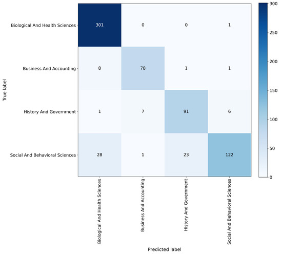
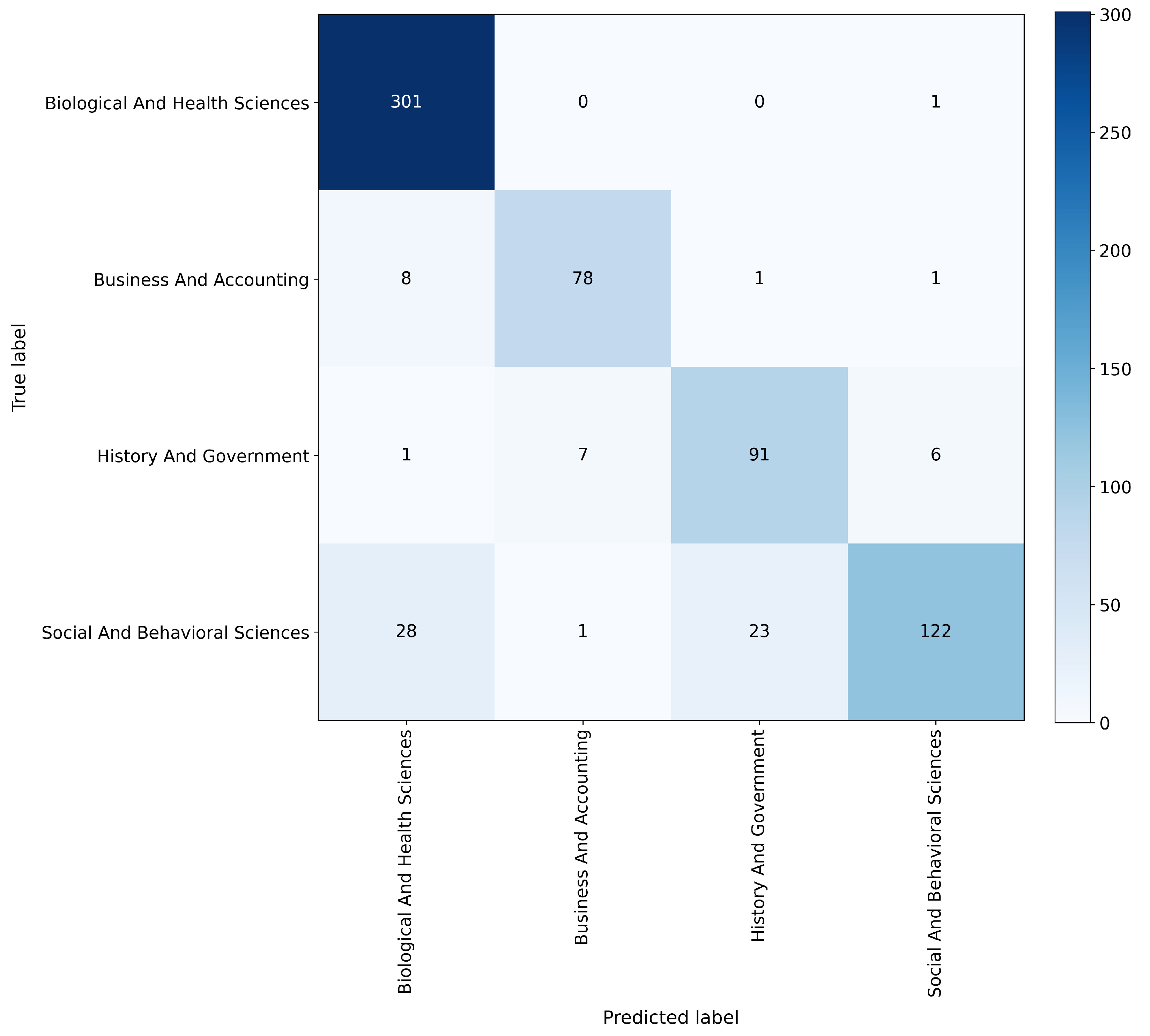
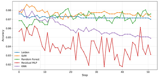
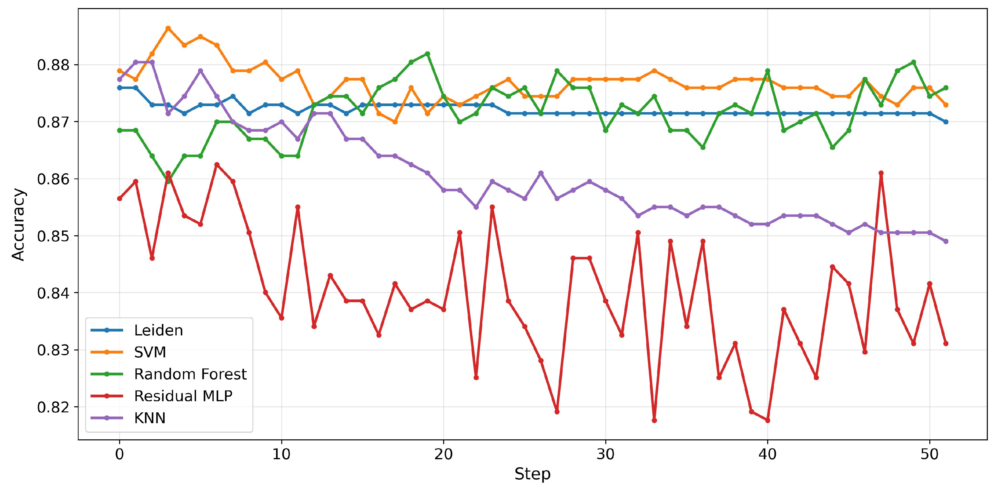
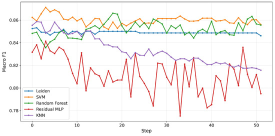
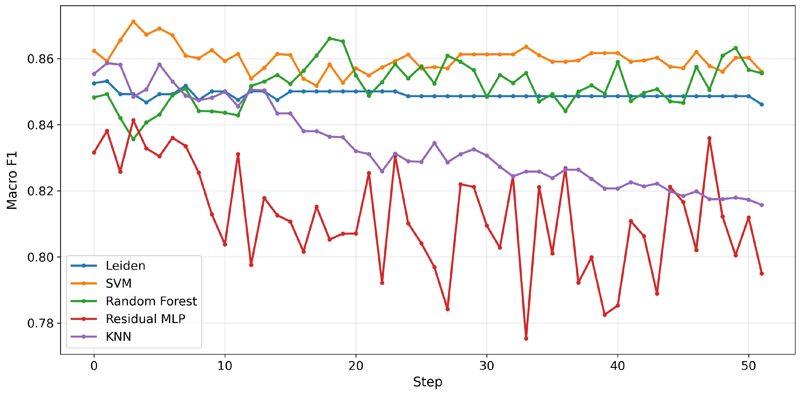
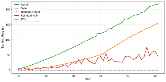
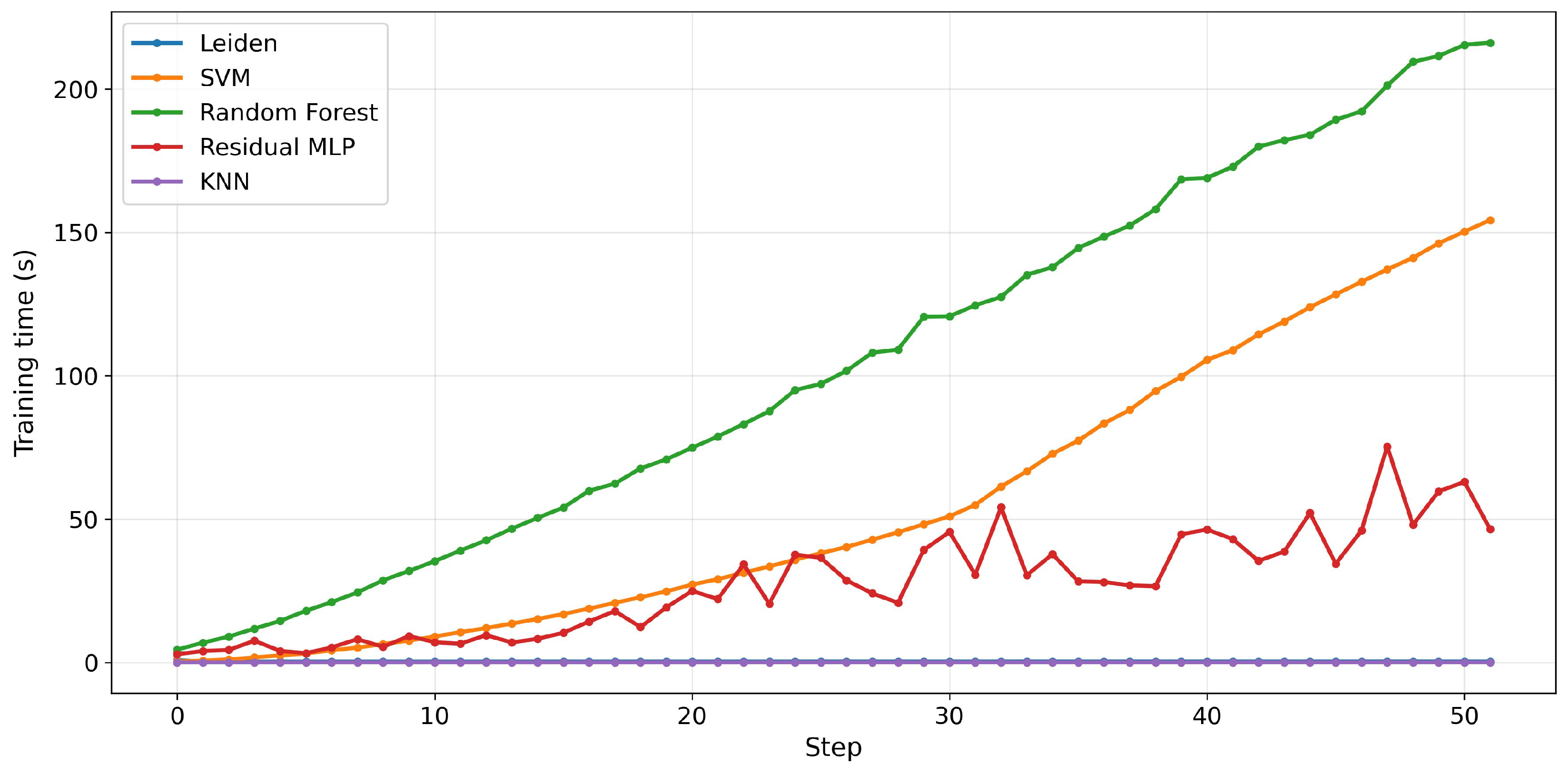
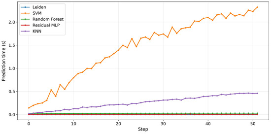
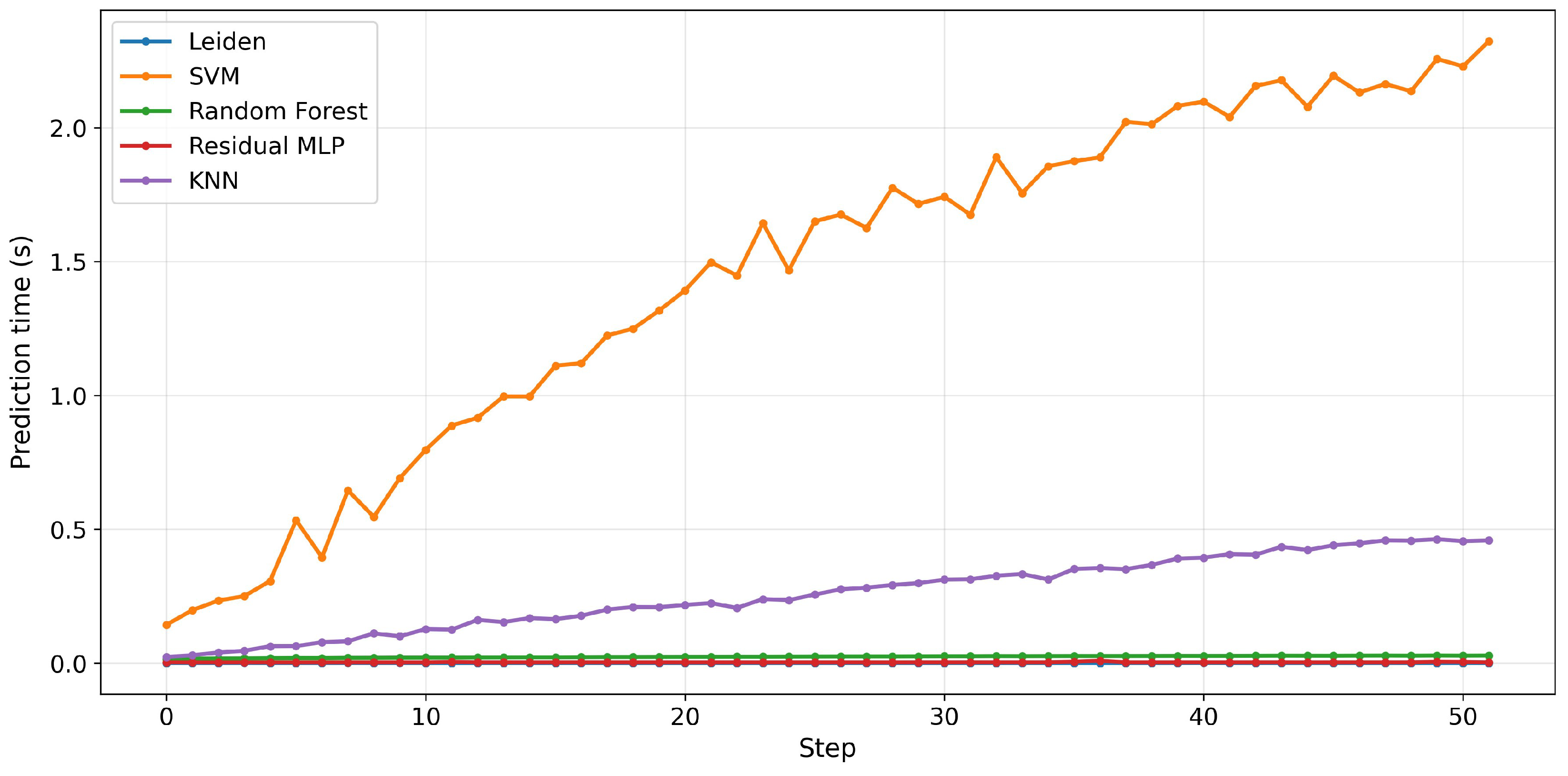
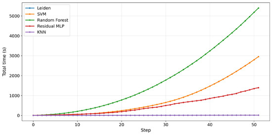
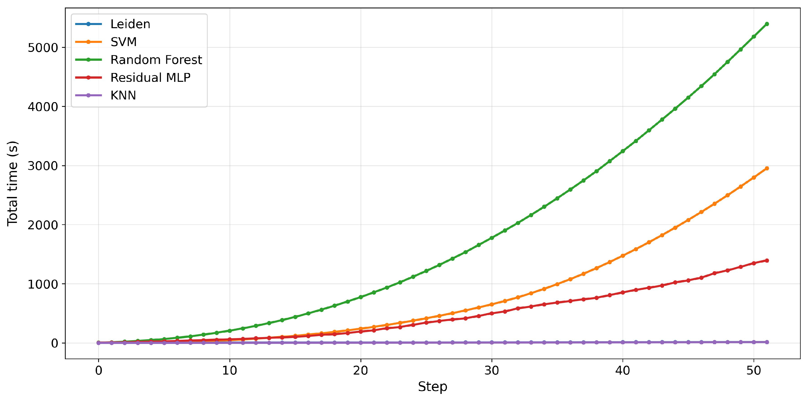
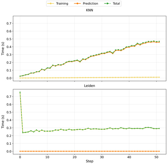
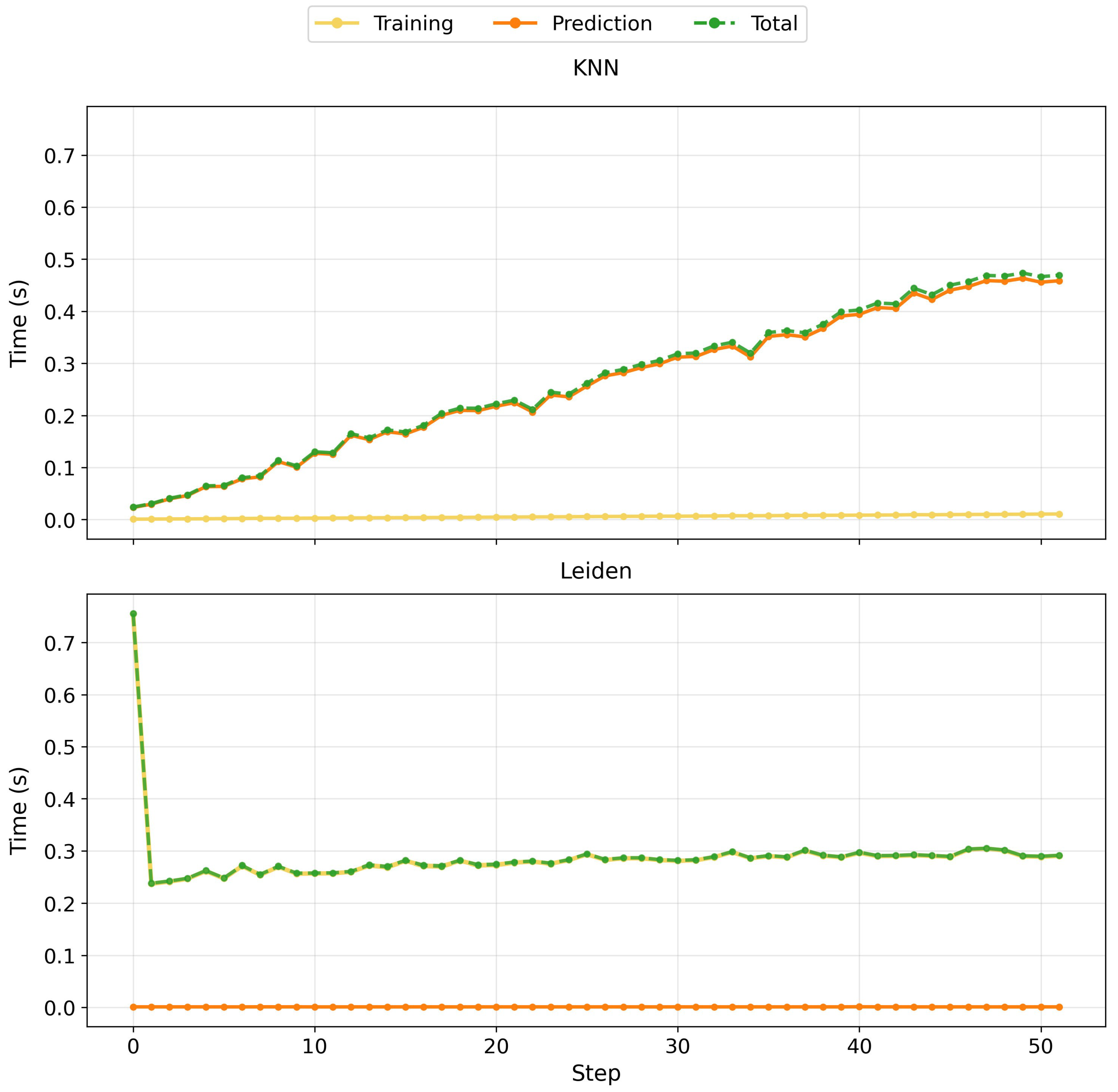
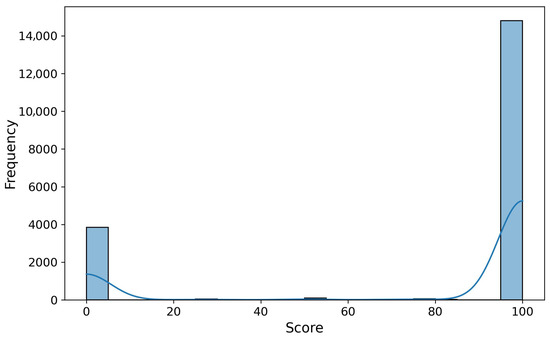
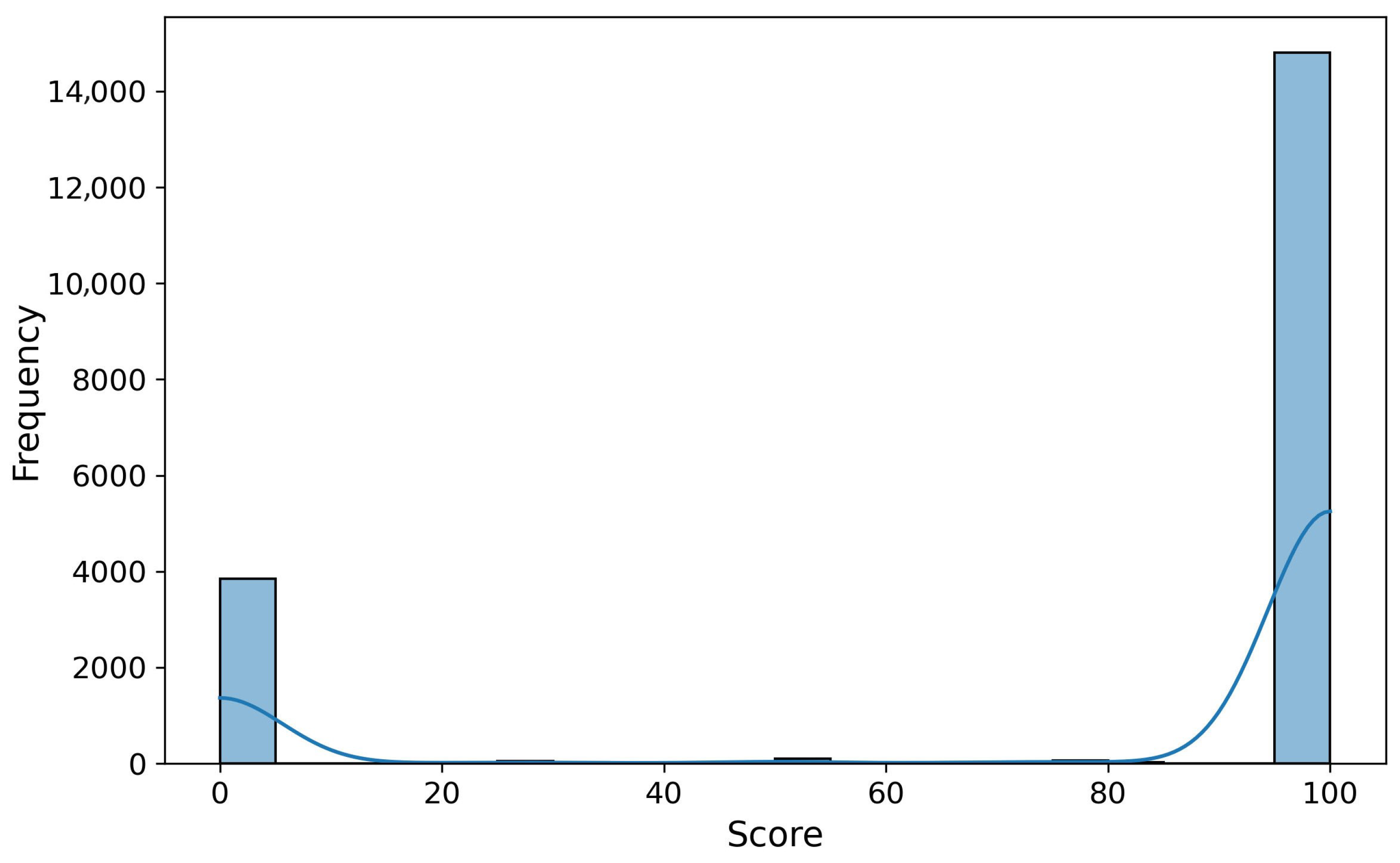
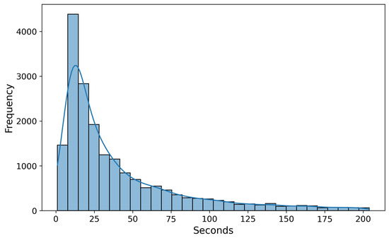
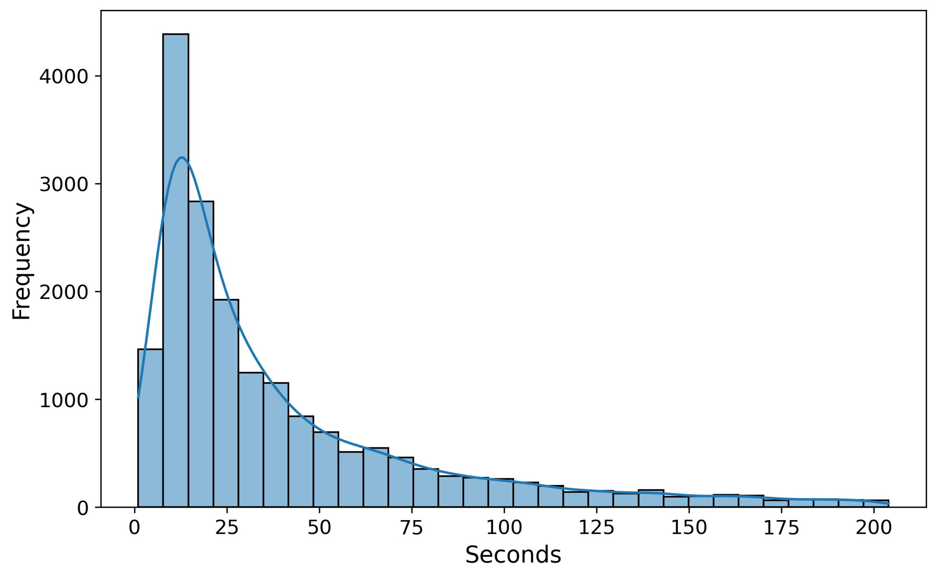
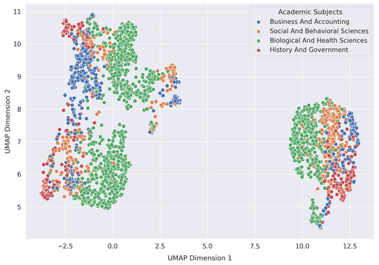
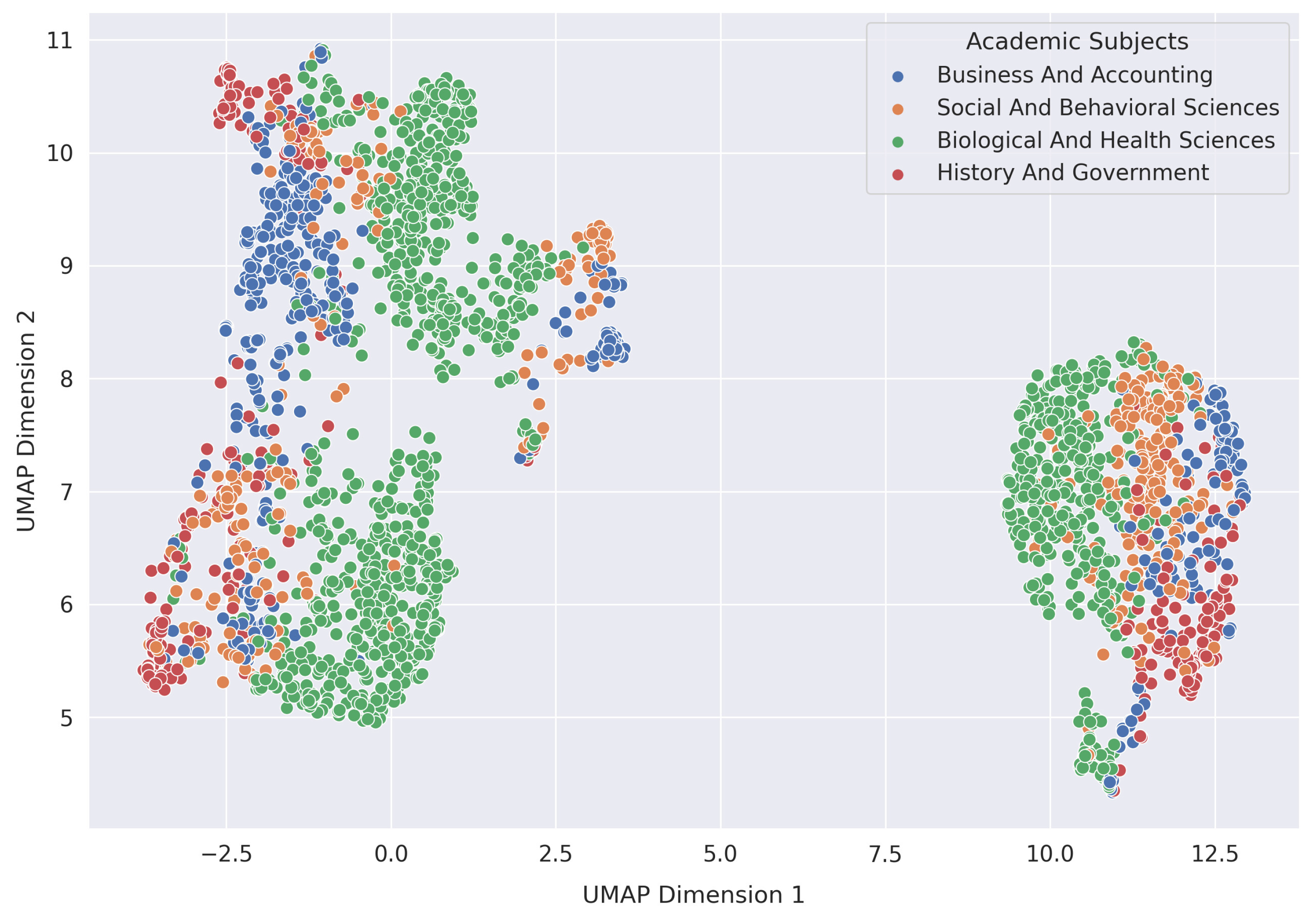
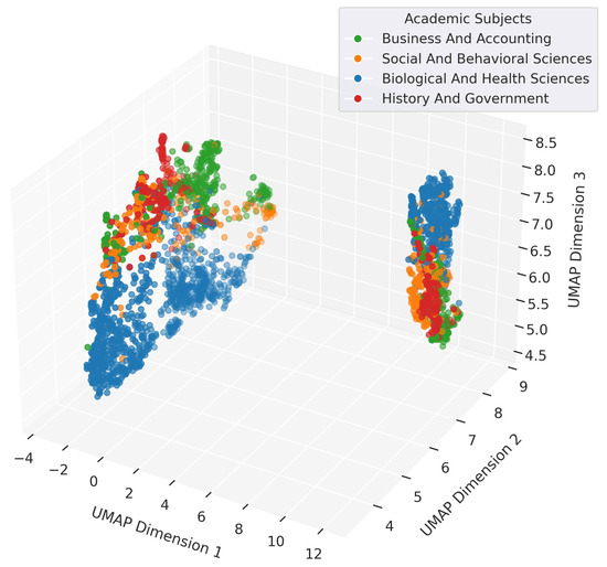
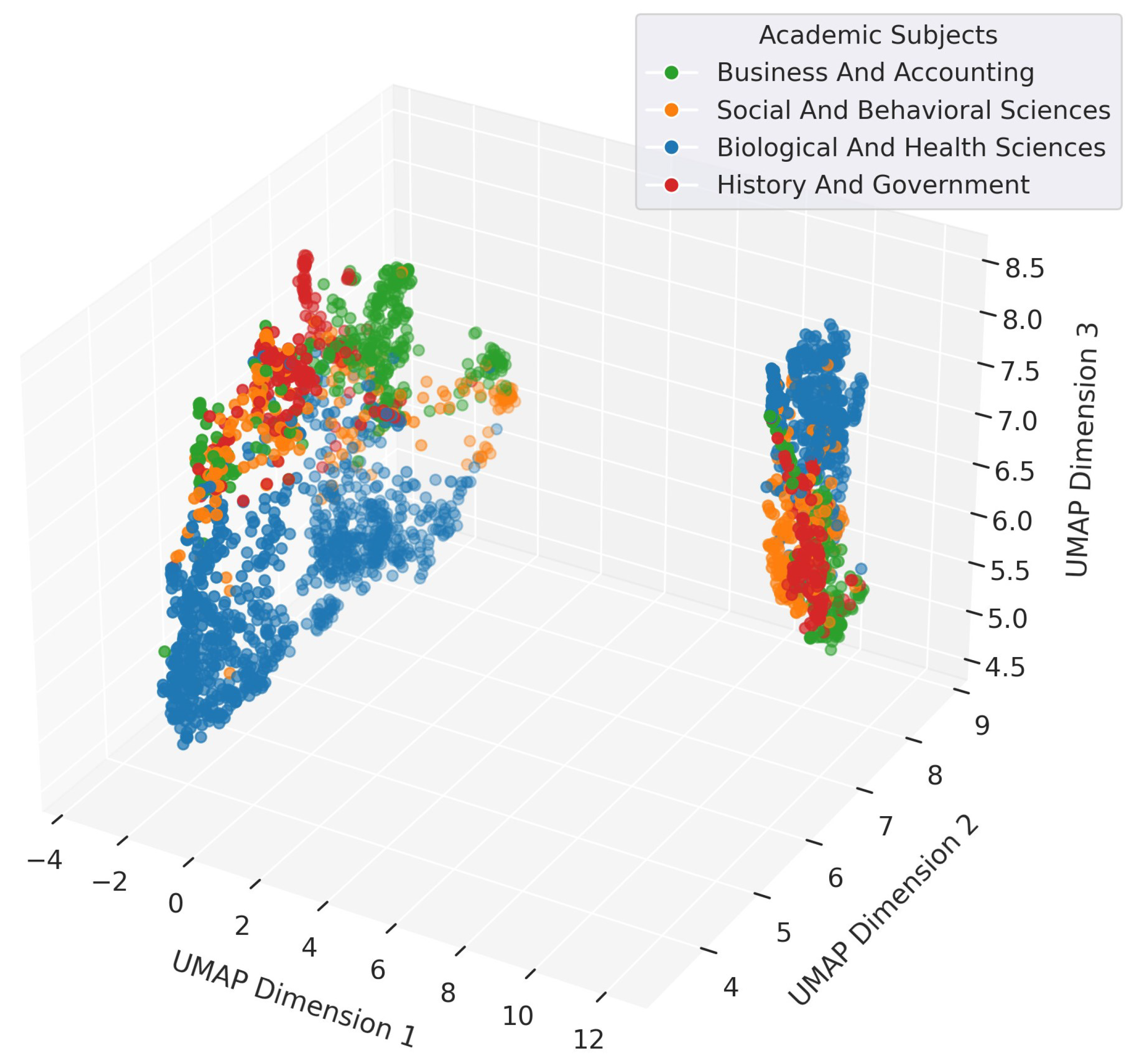
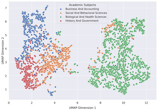
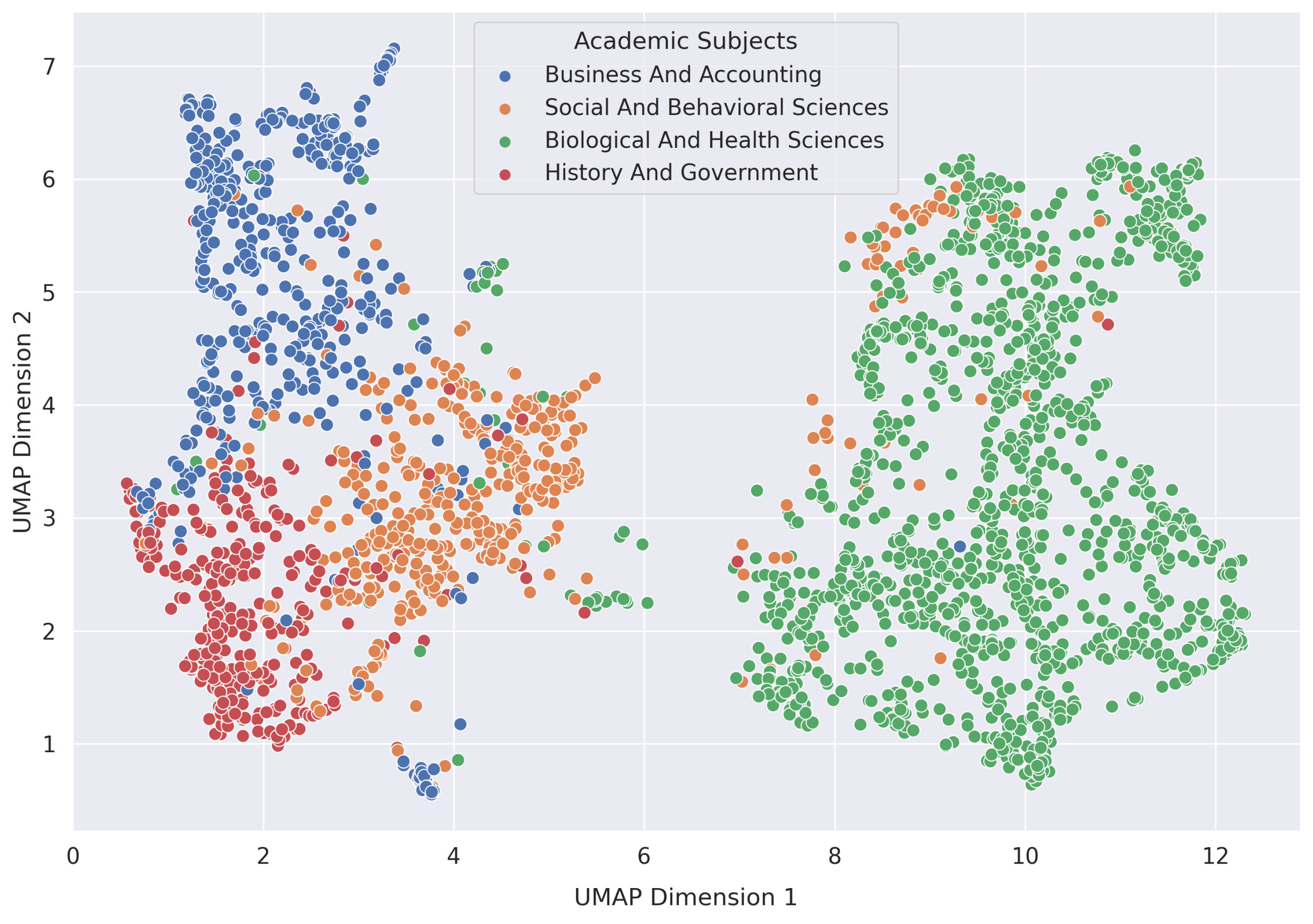
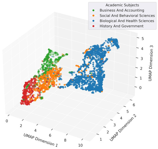
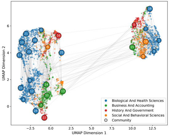
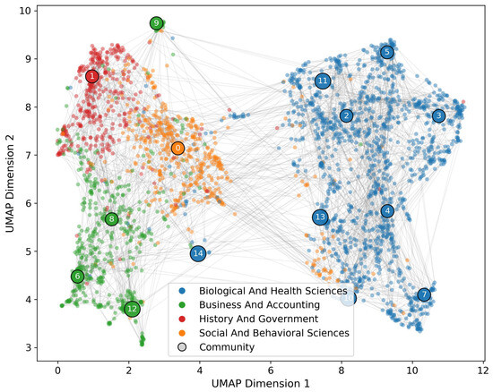
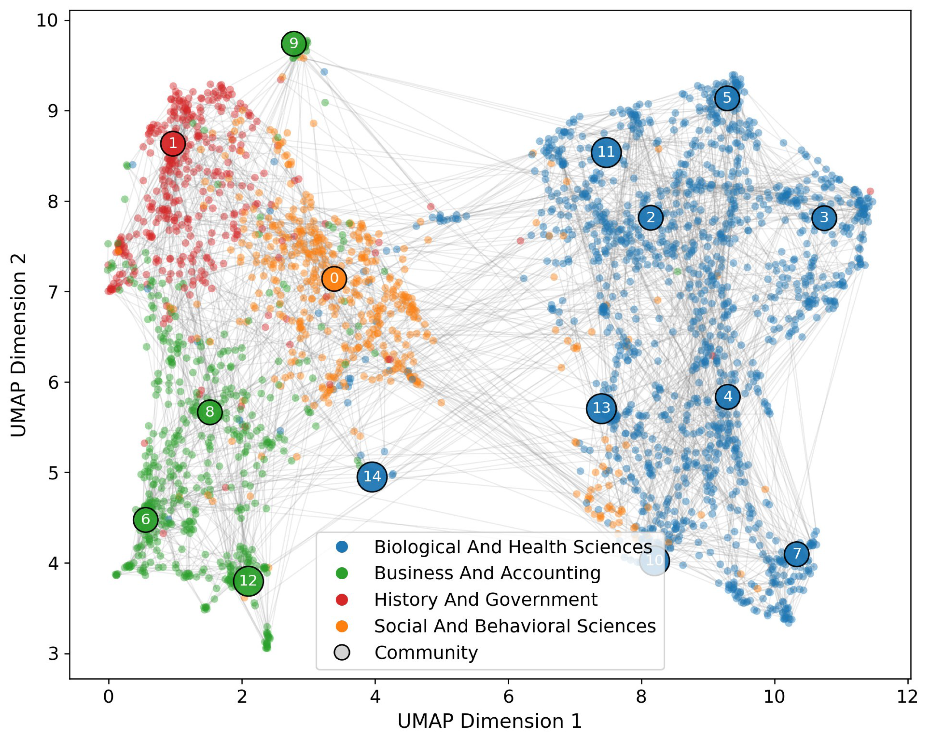
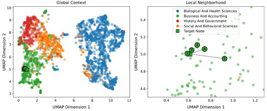
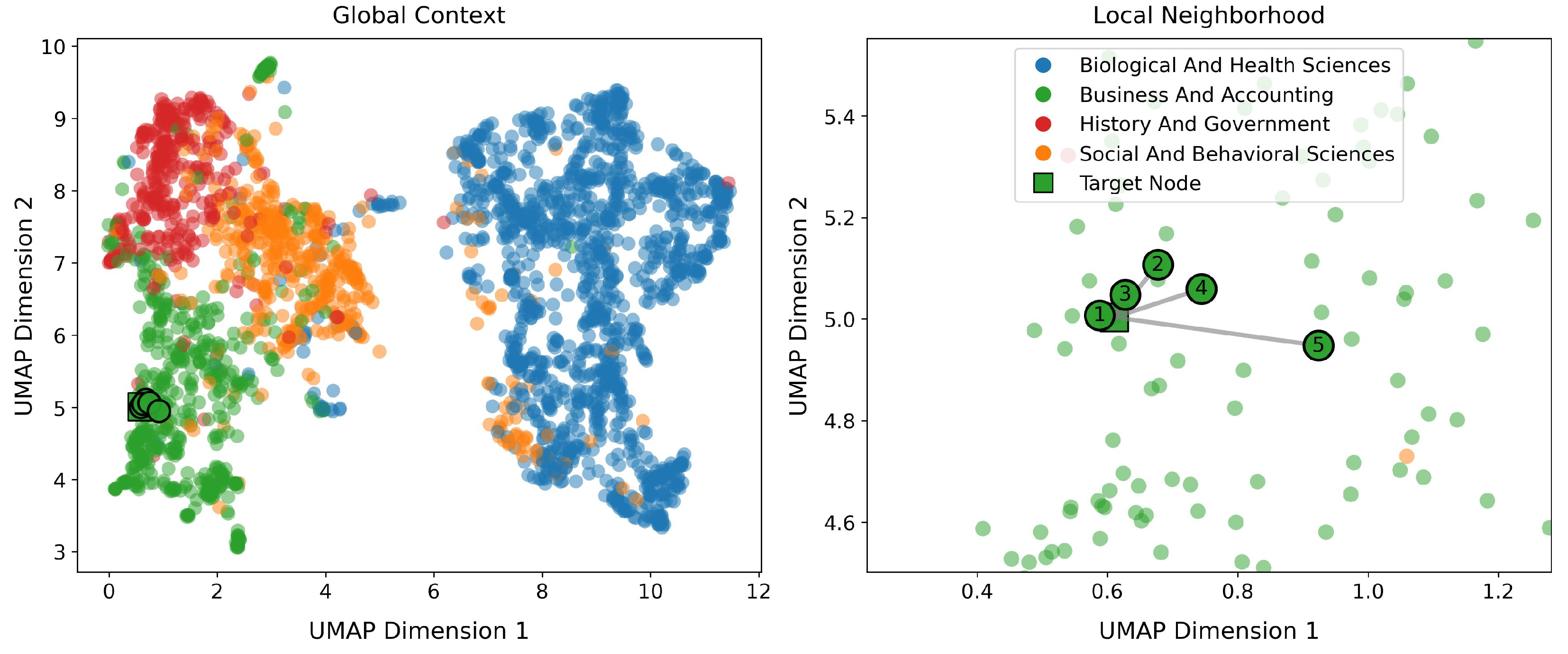
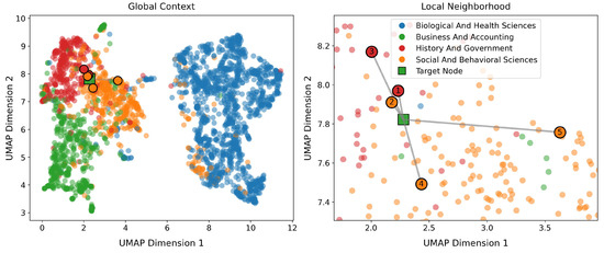
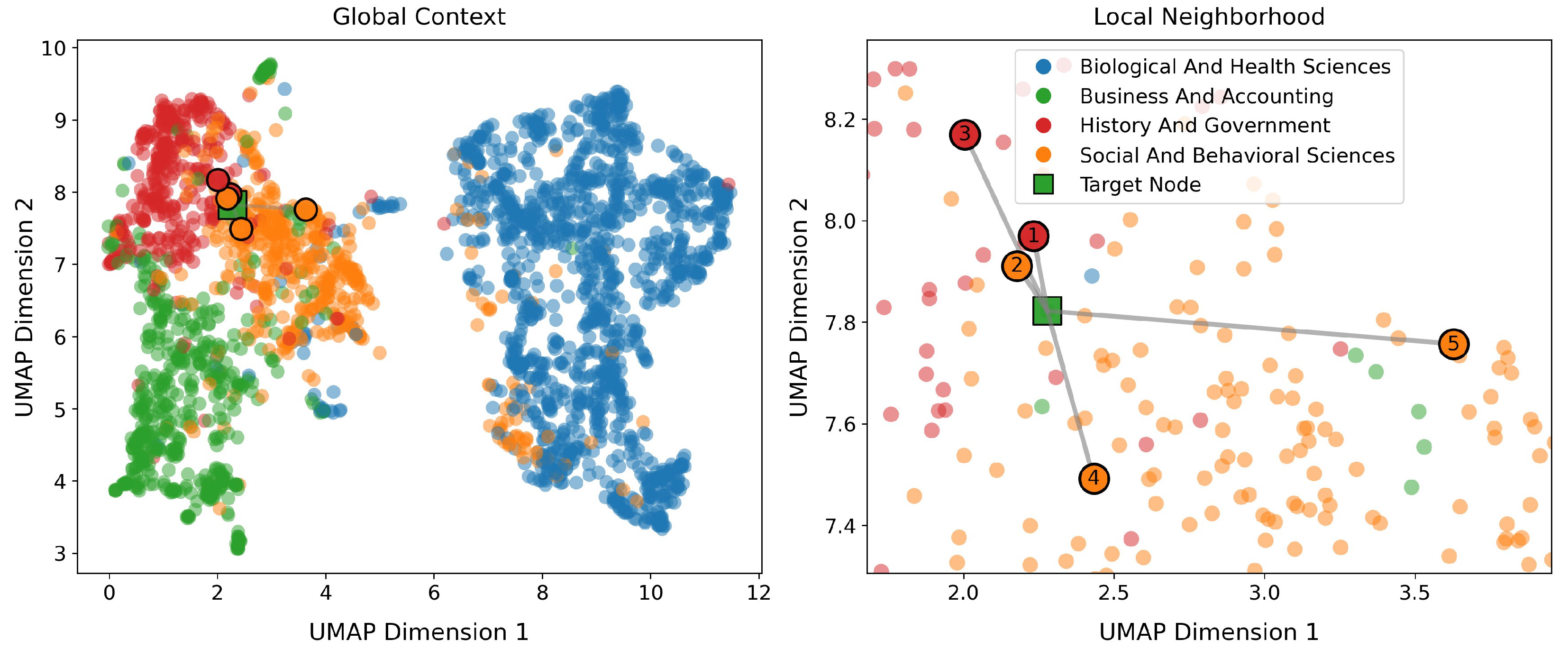
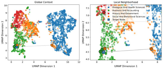
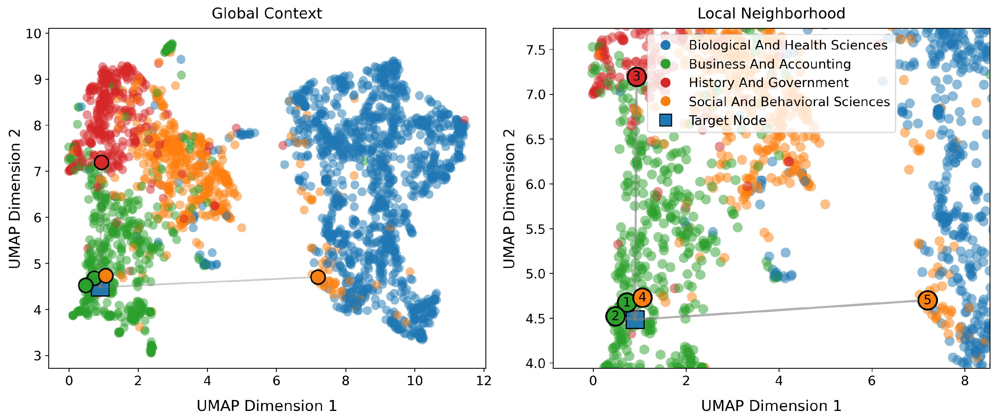

Disclaimer/Publisher’s Note: The statements, opinions and data contained in all publications are solely those of the individual author(s) and contributor(s) and not of MDPI and/or the editor(s). MDPI and/or the editor(s) disclaim responsibility for any injury to people or property resulting from any ideas, methods, instructions or products referred to in the content. |
© 2026 by the authors. Licensee MDPI, Basel, Switzerland. This article is an open access article distributed under the terms and conditions of the Creative Commons Attribution (CC BY) license.