


Abstract
The remaining useful life (RUL) prediction of lithium-ion batteries remains challenging for hybrid models due to high computational redundancy and hyperparameter sensitivity under complex operating conditions. To address these issues, this paper proposes a novel hybrid framework that integrates a CNN–BiLSTM–Attention network with a Crested Porcupine Optimizer (CPO). The key innovation lies in the simultaneous co-optimization of model structure and parameters: a group-level structured pruning strategy eliminates redundant convolutional kernels to reduce complexity, while the CPO algorithm dynamically optimizes critical hyperparameters (e.g., BiLSTM hidden nodes, attention dimensions) using RMSE as the fitness function. This dual optimization achieves a balance between model lightweighting and predictive accuracy. Experimental results on real-world electric vehicle datasets demonstrate that the optimized model reduces Mean Absolute Error (MAE) and Root Mean Square Error (RMSE) by 60.7% and 55.2%, respectively, compared to the baseline CNN–BiLSTM–Attention model. Furthermore, the model maintains high robustness across multiple datasets (R2 > 0.996), validating its strong generalization capability in small-sample and high-noise scenarios.
1. Introduction
Lithium-ion batteries serve as the primary medium [1] for electrochemical energy storage and are essential to the advancement of the new energy vehicle sector [2,3,4]. The New Energy Vehicle Industry Development Plan (2021–2035) establishes a clear objective [5] regarding the proportion of new energy vehicle sales by the year 2025. Due to their high energy density [6] and extended cycle life [7], lithium-ion batteries have emerged as the preferred choice for electric vehicle power sources.
Lithium-ion batteries have become the cornerstone of electrochemical energy storage, particularly propelling the advancement of new energy vehicles. Accurately predicting their remaining useful life (RUL) is paramount for optimizing energy distribution, ensuring operational safety, and facilitating predictive maintenance [8,9,10]. This capability holds significant technological value across diverse applications, from electric vehicles to grid-scale energy storage systems, where high reliability is demanded [11].
Research undertaken both nationally and internationally regarding the prediction of remaining useful life (RUL) for lithium-ion batteries has categorized the prevailing methodologies into two main types: model-based approaches and data-driven approaches [12].
Model-based prediction methodologies predominantly emphasize the examination of physicochemical characteristics of internal constituents of lithium-ion batteries. This is achieved through thorough investigations of these materials, which subsequently facilitate the formulation of analytical models [13]. Within this framework, three primary methodologies have been delineated: the degradation mechanism model, the equivalent circuit model, and the empirical recession model. For example, Lyu G et al. [14] proposed a RUL prediction method for lithium-ion batteries based on the Lebesgue sampling framework and similar sample fusion, which improves early prediction accuracy by the PCC-EuD optimization index, but relies on parameter optimization and has high computational complexity; Seyit Emre Özcan et al. [15] analyze the impact of the number of parallel RC networks on the SOC estimation of lithium-ion batteries by comparing the performance of 1RC, 2RC, and 3RC equivalent circuit models under US06 and UDDS driving cycles. However, this approach necessitates precise measurement data from sophisticated instruments and is hindered by complexities related to model intricacy and challenges in parameter updating. Similarly, Gangui Yan et al. [16] developed a Davignan equivalent circuit to enhance predictive accuracy; however, the process of dynamic parameter identification remains complex. Overall, these methodologies are susceptible to prediction inaccuracies stemming from deficiencies in mechanism modeling.
Data-driven methodologies emphasize the examination of chemical reactions occurring within batteries; however, this approach is constrained by the intricate nature of modeling underlying reaction mechanisms [17,18]. In contrast, contemporary techniques estimate the remaining useful life (RUL) of batteries by circumventing the dependence on mechanistic modeling. Instead, these methods focus on the analysis of historical operational data and the application of advanced algorithms, such as time series models, artificial neural networks, support vector machines, and correlation vector machines. For instance, Zhengyi Bao et al. propose a GRU-based spatial–temporal attention network that effectively estimates lithium battery RUL by capturing critical spatial–temporal features, but the raw data were not preprocessed, resulting in limited accuracy [19]. Longfei Wang et al. proposed a TCN-BiLSTM and ECM-based method for early fault diagnosis of lithium batteries by generating failure data via an equivalent circuit model to accurately identify internal short circuits [20]. Zhu Y. F. et al. developed a bidirectional long short-term memory (BiLSTM) model and incorporated backpropagation connections, resulting in a reduction in prediction error by 9% to 15%. However, the model still exhibits limitations in adequately decomposing data features [21]. Yu J et al. proposed a data-driven approach based on Adaptive Gaussian Mixture Model (AGMM) based data-driven approach, which learns the dynamic changes in battery sensor data and quantifies the health state degradation through online learning, but relies on feature extraction and adaptive adjustment of model structure [22]. Yang Z et al. proposed a data-driven hybrid model based on EEMD-GWO-SVR to predict the battery life, which improves the prediction accuracy through modal decomposition but the applicability to the dynamic working conditions still needs to be verified [23]. Similarly, Chen et al. [24] developed a hybrid framework integrating variational mode decomposition, an improved sparrow search algorithm, and multi-kernel support vector regression for accurate SOH and RUL prediction. Afshari S. et al. proposed a general method based on differential capacity and potential voltage curve feature extraction and sparse Bayesian learning (SBL) for early high-precision prediction of remaining useful life (RUL) for batteries, which outperforms current mainstream algorithms in performance [25]. Ali A. Osman et al. demonstrate the effectiveness of a support vector machine regression model, trained on normalized real-world battery data and validated through MATLAB R2014a simulation environment and Python scripting, for accurately estimating battery state-of-charge (SOC) under varying environmental conditions [26]. Dexin Gao et al. integrated a one-dimensional convolutional neural network with a bidirectional short-term memory network, thereby improving predictive performance by extracting depth information from capacity data through the one-dimensional convolutional neural network [27]. Xu et al. proposed a gray particle filter model with recursive least-squares parameter estimation to improve the accuracy of remaining service life prediction [28]. C. Bian et al. propose a stacked bidirectional long- and short-term memory neural network, which captures long-term dependencies in the degradation of batteries through bidirectional time series feature extraction. Its bidirectional information fusion mechanism significantly enhances the accuracy of state-of-charge (SOC) estimation in scenarios characterized by varying temperatures [29]. Jia Z et al. propose a lithium-ion battery remaining life prediction method based on a combination of convolutional neural networks and deep bidirectional long short-term memory networks, which solves the problem of poor prediction performance caused by insufficient historical data samples for training [30]. Wu et al. [31] propose a CNN-GRU-PF fusion model that integrates convolutional neural networks and gated recurrent units with particle filter, and employs a moving window to iteratively update the training set for enhanced RUL prediction accuracy. Catelani et al. propose a hybrid method that combines state monitoring and physical modeling. By combining recurrent neural networks (RNNs) with state space estimation techniques and utilizing genetic algorithms to optimize network performance, the method aims to improve the accuracy and robustness of predicting the remaining useful life (RUL) of lithium-ion batteries. This method was validated using the NASA battery degradation dataset and compared with the commonly used dual exponential empirical model and the innovative single exponential degradation model with fewer parameters and better performance [32], and empirical studies indicate that this architectural design enhances the capacity for fitting degradation trends by utilizing bidirectional memory units, thereby surpassing the performance of conventional single-path models in both RUL prediction efficiency and generalization capabilities. This data-driven approach to RUL prediction for lithium-ion batteries eliminates the necessity for developing intricate battery models, resulting in a straightforward computational process that facilitates real-time monitoring of battery status and enables online diagnosis of battery faults [33].
Existing methodologies for RUL prediction are primarily categorized into model-based and data-driven approaches. Model-based methods rely on precise physicochemical characterization and often suffer from computational complexity, challenges in parameter identification and updating, and inherent inaccuracies due to incomplete mechanistic modeling. Conversely, data-driven approaches, including models like LSTM, BiLSTM, and CNN–BiLSTM, circumvent the need for explicit mechanism modeling by learning from historical operational data. Despite their promise, these methods still face several critical limitations: (1) limited generalization under small-sample, high-noise conditions, leading to overfitting; (2) inadequate multi-scale feature synergy, where local degradation patterns and global temporal dependencies are not effectively captured and fused; (3) high sensitivity to hyperparameters, with traditional optimizers (e.g., PSO, GA) prone to premature convergence and suboptimal performance; (4) high computational complexity, which hinders deployment in resource-constrained scenarios.
Although the aforementioned hybrid models have improved prediction performance, they still face several critical challenges that hinder their practical application: (1) high computational complexity and overfitting risk due to redundant parameters in manually designed architectures; (2) sensitivity to hyperparameters, requiring extensive manual tuning that is inefficient and suboptimal; (3) inherent conflict between model lightweightness and accuracy, as most studies focus on either structure compression or parameter optimization, but rarely on both in a unified automated framework. This gap highlights the urgent need for an intelligent optimization mechanism that can co-optimize the model’s structure and parameters simultaneously.
To mitigate these challenges, we propose a hybrid prediction model that synergistically combines convolutional neural networks (CNN), bidirectional long short-term memory networks (BiLSTM), and an aattention mechanism, with the entire framework being optimized by the Crested Porcupine Optimization (CPO) algorithm. Specifically, the CNN is employed to extract local degradation features from capacity sequences, the BiLSTM captures global bidirectional temporal correlations, and the attention mechanism dynamically emphasizes critical information during key decline stages.
The selection of an appropriate optimization algorithm is of paramount importance for the efficacy of the proposed hybrid model. While conventional optimizers such as Particle Swarm Optimization (PSO) and genetic algorithm (GA) have been extensively applied in the literature, they are inherently limited by premature convergence and a high degree of sensitivity to parameter configurations. These shortcomings frequently lead to suboptimal solutions when optimizing within the complex, high-dimensional search spaces characteristic of deep learning hyperparameters and structured pruning ratios.
The Crested Porcupine Optimizer (CPO) is a novel metaheuristic that dynamically balances exploration and exploitation, adaptively manages population diversity, and is less sensitive to initial parameter settings—making it well-suited for optimizing the high-dimensional structure–parameter space of hybrid neural networks.
These capabilities make CPO particularly effective for optimizing the high-dimensional “structure–parameter” joint space of the CNN–BiLSTM–Attention model, which involves both discrete pruning decisions and continuous hyperparameter adjustments.
In recent years, hybrid models such as CNN–BiLSTM–Attention have been widely applied in battery health status and remaining life prediction. For example, Tian et al. [34] propose a lithium battery health status prediction model based on CNN–BiLSTM–AM, demonstrating its advantages in feature extraction and time series modeling; however, their model does not incorporate any structural optimization, leading to redundant parameters and high computational complexity. Quan et al. [35] optimized the CNN–BiLSTM–AT model using an enhanced whale optimization algorithm, further improving the prediction accuracy of fuel cell remaining lifespan; nevertheless, their optimization is confined to hyperparameters and does not address model structure compression. In contrast, the proposed method introduces a group-level structured pruning strategy within the CPO framework, enabling simultaneous optimization of both model structure and hyperparameters. This joint optimization not only enhances prediction accuracy but also significantly reduces computational complexity, overcoming the limitations of existing methods. To address the identified research gaps—namely, the lack of a unified framework for simultaneous structure compression and parameter optimization—this paper proposes a novel optimization framework with three core innovations that collectively overcome the limitations of prior work:
Algorithmic Application Innovation: Existing hybrid models either rely on manual hyperparameter tuning or use traditional optimizers (PSO, GA) that suffer from premature convergence in high-dimensional, mixed-variable spaces. We propose a novel application of the Crested Porcupine Optimizer (CPO) for the simultaneous optimization of both hyperparameters (BiLSTM hidden nodes, attention dimensions) and structural parameters (group-level structured pruning ratios). CPO’s four-stage defense strategy dynamically balances exploration and exploitation, effectively navigating the joint search space and avoiding local optima—a capability absent in prior optimizers.
Structural Optimization Innovation: Unlike conventional post-training pruning methods that treat compression as a separate step after training, we implement a group-level structured pruning strategy guided by a dependency model and a regularized importance assessment criterion. This strategy is dynamically integrated within the CPO loop, ensuring that pruning decisions are co-optimized with hyperparameters to directly minimize prediction error while reducing complexity. This overcomes the limitation of sequential approaches that often sacrifice accuracy for efficiency.
Framework Innovation: We develop an integrated “feature extraction-sequence modeling-weight distribution-adaptive tuning” framework. By using RMSE as the fitness function, the CPO orchestrates both pruning and hyperparameter tuning to create a closed-loop optimization system. This holistic approach results in a model that is both highly accurate (60.7% MAE reduction) and lightweight (57.7% parameter reduction), suitable for deployment in resource-constrained environments—an outcome not achievable by prior methods that optimize only one aspect.
The following sections of this paper are organized in the manner outlined below: Section 1 delineates the principles and implementation of the Crested Porcupine Optimization (CPO) algorithm. Section 2 outlines the design of the CNN–BiLSTM–Attention hybrid model. Section 3 provides experimental validation and performance analysis. Finally, Section 4 offers a comprehensive summary of the entire text.
2. Principles and Implementation of the CPO Algorithm
The Crested Porcupine Optimization Algorithm (CPO) [36] draws inspiration from the four-tiered defensive repertoire of the crested porcupine (CP), ranging from visual and auditory signals to olfactory and physical attacks. These behaviors are mapped onto the algorithm’s search strategies, with the less aggressive visual and auditory defenses facilitating exploration, and the more aggressive olfactory and physical defenses driving exploitation. A distinguishing feature of CPO is its cyclic population reduction mechanism, which emulates the selective activation of defenses observed in nature—only CPs that perceive a threat engage their defensive responses. This approach strategically balances convergence speed and population diversity throughout the optimization process.
To ensure clarity, this section may be divided by subheadings. It should concisely present the experimental results, followed by their interpretation and a summary of the conclusions that the data support.
2.1. Population Initialization and Search Strategy
In a manner akin to other algorithms that utilize meta-heuristic populations, the CPO algorithm initiates the search process with a preliminary collection of individuals, which represent potential solutions.
where denotes the number of individuals (population size ), is the i candidate solution in the search space, and and denote the lower and upper boundaries of the search range, respectively. The term represents a random vector, with each element independently drawn from a uniform distribution between 0 and 1.
2.2. Dynamic Population Optimization Strategies
This methodology simultaneously improves convergence rate and maintains population diversity by mimicking a natural defense mechanism: only those candidate solutions (CPs) that perceive a threat activate the defensive response. Accordingly, during the optimization process, a subset of CPs is temporarily withdrawn from the population to promote faster convergence. These individuals are subsequently reintegrated to bolster population diversity and mitigate the risk of premature convergence to local minima. The iterative execution of this process is regulated by a cyclic variable , which defines the optimization schedule and is mathematically formulated as follows:
where is the predefined maximum number of cycles, denotes the current iteration (function evaluation) count, specifies the maximum allowable number of function evaluations, and defines the minimum required population size, acting as a lower bound to maintain population diversity and prevent the newly generated population from falling below this threshold.
2.2.1. The First Defense Strategy
Use normal distribution to generate random values and mathematically simulate these options. If these random values are less than 1 or greater than −1, it is encouraged to approach . Otherwise, the predator will stay away from .
where is the optimal solution identified at iteration , is a vector that defines the predator’s position derived from the current and a randomly selected population member, is a normally distributed random variable, and is a random number uniformly distributed on the interval [0, 1].
2.2.2. The Second Defense Strategy
This strategy mimics the porcupine’s defensive behavior of producing sounds to deter predators, where the sound volume increases as the predator approaches. The mathematical formulation of this behavior is given as follows:
where and are two random integers between [1, N] and is a random value generated between 0 and 1.
2.2.3. The Third Defense Strategy
Following the standard CPO algorithm, this strategy mathematically simulates the odor secretion behavior. The formulation is given by Equation (5):
where is a random number between [1, N] and is a parameter used to control the search direction. is the position of the individual in iteration , and is the defense factor. is the random value in the interval [0, 1] and is the odor diffusion factor.
Compared with GA, which mixes parental genes through crossover operation, mutation provides randomness. The CPO odor defense strategy, as defined in Equation (5), utilizes a dynamically calculated odor factor based on fitness, enabling non-crossover directional learning by generating a strong attraction field around high-fitness individuals.
2.2.4. The Fourth Defense Strategy
Similarly, the fourth defense strategy (physical attack) in the standard CPO algorithm is formulated as Equation (6):
where is the best solution obtained, representing the position of the individual of in iteration , representing the predator at that position; is the convergence rate factor, as defined in the parameter settings; is a random number uniformly distributed in [0, 1]; and is the average force acting on the I predator due to .
PSO speed update:
where is the inertia weight, and are the acceleration constants, and the maximum learning step is adjusted. and are two random functions with a value range of [0, 1] to increase the randomness of search. and are local and global optimal positions.
PSO plays an important role in the convergence of the algorithm. The larger its value, the wider the scope of particle leap, and it is easier to find the global optimum, but it will also miss the ability of local search. Compared with the PSO algorithm, which relies on the historical optimal position and is prone to premature convergence, CPO’s physical attack strategy introduces inelastic collision force and defense attenuation factor , adding reverse disturbance when reaching the optimal solution to suppress premature convergence.
In the proposed co-optimization framework, the four defense strategies of CPO are assigned distinct roles in exploring and exploiting the hyperparameter space and structural parameters. Specifically, the first defense strategy (visual), characterized by global jumps, is primarily responsible for exploring continuous hyperparameters such as the learning rate and regularization coefficient. The second defense strategy (sound), which performs local searches, is employed to optimize discrete parameters, including the number of BiLSTM hidden neurons and the key/value dimensions of the attention mechanism. The third defense strategy (odor) creates an attraction field around high-fitness individuals to guide the optimization of the pruning ratio—the proportion of convolutional kernels to be retained. Finally, the fourth defense strategy (physical attack) refines the solutions already found, ensuring a fine balance between model lightweightness and predictive accuracy. This explicit assignment enhances the transparency of the optimization process and clarifies how each defensive behavior contributes to the final model performance.
The following is a core comparison table (Table 1) between CPO and mainstream optimizers (PSO, GA), highlighting the unique advantages and innovative points of CPO. The table structure focuses on five key dimensions, making it easy to intuitively understand the differentiated value of CPO:
Table 1.
Comparison of CPO with PSO and GAs.
The comparative analysis in Table 1 substantiates the suitability of CPO for our specific task of co-optimizing the CNN–BiLSTM–Attention model. The optimization problem we face is characterized by a high-dimensional, mixed-variable search space, involving both discrete (e.g., pruning ratios, number of neurons) and continuous (e.g., learning rate) parameters. Traditional optimizers like PSO are prone to premature convergence in such complex spaces, while GA often suffers from high coding complexity and sensitive parameter tuning.
CPO addresses these challenges through its biologically inspired mechanisms. The first (visual) and second (sound) defense strategies facilitate global exploration of the hyperparameter landscape, preventing the solution from getting trapped in local optima early on. The third (odor) strategy, with its fitness-based attraction field, is particularly effective for guiding the discrete pruning ratio decisions towards an optimal balance be-tween model compactness and accuracy. Finally, the fourth (physical attack) strategy re-fines the solution locally, ensuring fine-tuned convergence. Coupled with its cyclic population reduction technique, CPO dynamically maintains population diversity, which is crucial for navigating the joint “structur–parameter” space without overfitting. This inherent ability to balance exploration and exploitation makes CPO a more robust and effective choice than PSO or GA for this application.
2.3. CPO Algorithm for Optimizing Time Series Networks
In summary, this investigation leverages the CPO algorithm to enhance a time series forecasting network, leading to the development of a novel CPO–time series algorithm. The complete procedural framework of the algorithm is depicted in Figure 1.
Figure 1.
CPO algorithmic optimization of time series network processes.
- (1)
- Develop the CNN–BiLSTM–Attention network and delineate its architecture, which should encompass the number of nodes in the hidden layers, the fitness function utilized by the neural network, and the activation function applied to the output nodes;
- (2)
- Initialize the parameters for the CPO algorithm, which includes defining the initial population’s position and velocity, as well as other relevant parameters such as population size, maximum iteration count, learning factor, and inertia weights;
- (3)
- Identify the optimal solution through the CPO algorithm. The fitness of each individual’s new position is assessed, and the current optimal solution is updated following the evaluation of all individuals. An individual is designated as the new optimal solution if its fitness value surpasses that of the existing optimal solution;
- (4)
- Compute the error. Update the positions and algorithm parameters of the remaining individuals, select training and testing samples, calculate the error value, and adjust the iteration count accordingly;
- (5)
- Ascertain whether the maximum iteration limit or the predetermined error criterion has been achieved. If neither the error nor the iteration count meets the specified requirements, reiterate steps 3 and 4 until the conditions are satisfied, with the final solution representing the optimal resolution to the problem;
- (6)
- Map the location of the optimal output solution to a weight matrix, which will serve as the weights from the implicit layer to the output layer within the time series network, thereby facilitating the realization of the CPO–time series model. Utilize the aforementioned method to determine the optimal solution and optimize network parameters;
- (7)
- Present the network training outcomes to establish a fitted model. Preprocess the data and input it into the trained CPO model for further analysis.
2.4. Performance Validation of CPO on Benchmark Functions
To demonstrate the effectiveness of the Crested Porcupine Optimizer (CPO) as an optimization algorithm, we evaluate it on two representative CEC2005 benchmark functions: F4 (unimodal) and F12 (multimodal). Figure 2 shows the convergence curves comparing CPO with Particle Swarm Optimization (PSO), the genetic algorithm (GA), and Gray Wolf Optimizer (GWO). On both functions, CPO achieves faster convergence and lower final fitness values, indicating its strong global search capability and suitability for complex optimization tasks such as the joint structure–parameter optimization in this study.
Figure 2.
Comparison of convergence curves of CEC2005 F4 and F12 functions (CPO vs. PSO, GA, GWO).
3. Optimizing the CNN–BiLSTM–Attention Hybrid Model Based on CPO
3.1. CNN–BiLSTM–Attention Model Architecture
This research presents a hybrid architecture that combines convolutional neural networks (CNN), bidirectional long short-term memory networks (BiLSTM), and an attention mechanism. This approach utilizes multi-scale feature fusion to improve the accuracy of predicting the remaining service life of lithium-ion batteries by co-optimizing features at multiple levels. The proposed model is structured into three primary components: a feature extraction layer, a temporal modeling layer, and a dynamic weight allocation layer, collectively forming a three-dimensional optimization system.
Firstly, the CNN is employed to extract local degradation patterns and spatial correlations from the original capacity sequences, while a group-level structured pruning strategy [37,38,39] is utilized to eliminate redundant convolutional kernel groups. This approach effectively reduces computational complexity without compromising the essential feature extraction capabilities. Secondly, the BiLSTM is implemented to establish a bidirectional temporal connection, enabling the simultaneous analysis of capacity decay trends across both historical and future time points. Lastly, a self-attention mechanism is incorporated to dynamically assess the significance of features at various time intervals.
These three components are integrated to create a multi-scale analysis framework characterized by a “local-global-critical point” approach. Furthermore, the model is enhanced through the application of the Crested Porcupine Optimization (CPO) algorithm, which facilitates the adaptive tuning of network hyperparameters.
3.2. Core Module Functional Design
3.2.1. Convolutional Neural Network (CNN)
The convolutional neural network (CNN) module facilitates effective feature extraction by employing local sensing and weight-sharing strategies. This module is structured in a three-tier architecture. At its core lies the convolutional layer, where depth-separable convolutional operations are executed utilizing a 1 × 1 convolutional kernel. Local feature extraction is accomplished as delineated in Equation (8).
where is the output of the channel of layer , is the channel of layer , is the input of the i-th channel of layer , is the weight of the convolution kernel, is the bias, and Relu denotes the activation function.
The pooling layer assesses the significance of the output features generated by the convolutional layer through the application of a pooling function. This process effectively disregards less critical subtle features, thereby enhancing the abstraction of the feature values.
The fully connected layer serves a crucial function following the convolutional and pooling layers, as it is designed to assign weights to the extracted features and to amalgamate various local features.
3.2.2. Attention Mechanism
In this paper, we introduce the self-attention mechanism in the CNN–BiLSTM architecture, the core idea of which is to dynamically assign attention weights by calculating the correlation of different time steps within a sequence, so that the model focuses on the historical information that contributes more to the prediction target.
- (a)
- Self-attention mechanism
- Query, Key, Value mapping: maps the input features to the query matrix , key matrix K, and value matrix , respectively.
- Attention score calculation: attentional weights were calculated by scaling dot product through Equation (9):where is the dimension of the key vector and the scaling factor is used to avoid gradient vanishing.
- Feature-weighted fusion: the value matrix is weighted according to the attention weights to generate a context-aware feature representation.
This standard attention layer, when embedded into BiLSTM, is capable of capturing long-range dependencies in the time series and highlighting key time-step features. However, the integration of these standard components (CNN, BiLSTM, Attention) often leads to a model with high computational complexity and redundancy. To address this, our key innovation lies in a novel group-level structured pruning framework, as detailed below.
- (b)
- Group-level structured pruning
To achieve precise and dependable outcomes, neural networks are frequently designed with deep architectures and a substantial number of neurons to improve data representation. Nonetheless, the contribution of certain neurons to the feature extraction process may be minimal. Instead of improving the accuracy of output, these neurons may result in considerable computational burden. Consequently, this study employs structured pruning to identify and eliminate neurons and connections that have a limited impact on the learning process, thereby streamlining network parameters and enhancing computational efficiency. Structured pruning is generally preferred over unstructured pruning, as it facilitates direct group pruning without necessitating specific accelerators to mitigate memory consumption.
Deep learning architectures are constructed from fundamental components, including convolutional layers, activation layers, and fully connected layers. The intricate interdependencies both among and within these components render the process of model pruning particularly complex. Consequently, when it becomes necessary to prune a segment of the network that has weight connections to other layers, it is imperative to carefully manage their interdependencies and significance; failure to do so may result in a substantial decline in the accuracy of the pruned model. Group-level structured pruning offers a straightforward and effective approach to delineate the relationships between layers and parameters, allowing for their accurate grouping to facilitate model simplification, as outlined below:
Neural networks can be distinctly categorized into several fundamental components according to their respective functions, as illustrated in Equation (10). Each component may correspond to a parameterized layer, including convolutional and fully connected layers, or to a non-parameterized operation, such as residual connectivity.
The interrelationships among the inputs and outputs of each component are clearly defined, and the network equations are restructured, as demonstrated in Equation (11). This formulation aids in the modeling of dependencies by classifying all relationships into two fundamental categories: inter-layer dependencies and intra-layer dependencies.
where denotes the dependency in layer , and denotes the dependency between the output of layer and the input of layer .
In networks characterized by a defined structure, interlayer dependencies between the upper and lower layers are invariably present. Given that and represent intermediate features of identical dimensions within the network, the estimation of dependencies between layers can be effectively derived from this attribute. Conversely, intra-layer dependencies necessitate the pruning of both the inputs and outputs of the layer. Many fundamental layers satisfy this criterion and employ a uniform pruning strategy within the layers. Although the output of a convolutional layer is contingent upon the input elements and the weights of the convolutional kernels corresponding to specific regions, the pruning strategies for its input and output layers typically differ. The pruning of the input to the convolutional layer primarily aims to diminish computational demands, whereas the pruning of the output is intended to modify the size of the feature map to align with the requirements of the subsequent layer. Consequently, based on Equation (12), a neural network dependency model that incorporates convolutional layers is formulated, as illustrated in Figure 3. The initial term of this model quantifies the inter-layer dependencies, while the subsequent term evaluates the intra-layer dependencies, which may incorporate either uniform or varied pruning strategies. This procedure ultimately results in the formation of a dependency graph for the entire network, anticipated to present as a sparse matrix with dimensions n × n.
where is a bool operation, then its result is 0 or 1; is a logical OR operation; is a logical AND operation; and is a pruning scheme.
Figure 3.
Example dependency diagram for a deep learning model with a convolutional neural network.
Upon acquiring the necessary dependencies, it is imperative to assess the significance of the grouping parameters prior to the execution of group-level structured pruning. To address the challenge of enhancing the importance of paradigms across various layers, which is hindered by distributional discrepancies, a regularization term is incorporated. This term facilitates the sparsification of the group-level weights, thereby allowing for the removal of groups with negligible importance from the network, thus completing the pruning process as delineated in Equations (13) and (14).
where denotes the weighting group, denotes the fine-tunable dimension, refers to the normalized score, refers to the contraction intensity , and m refers to the importance of the m-optimizable dimension.
In this paper, group-level structured pruning is used to compress the model size and improve the inference efficiency by removing convolutional kernels or neurons with smaller contributions. The specific process is as follows:
- Dependency modeling
Inter-Layer Dependency: the output feature maps of the convolutional layers need to be matched with the input dimensions of the next layer, and pruning needs to synchronize the number of channels of the adjacent layers.
Intra-layer dependency: the input and output channels of the convolutional kernel are coupled through the weight matrix, and pruning needs to ensure the completeness of the parameter set (Equations (10)–(12)).
- 2.
- Importance assessment and dynamic pruning
L1 Paradigm Importance: the absolute sum of the weights of the convolution kernel is computed and the low importance channels are filtered as shown in Equation (15).
where refers to the importance weight and to the convolution kernel weight.
Sparse Regularization: the model is further simplified by guiding the sparsification of group-level weights through the L1 regular term (Equations (13) and (14)).
- 3.
- Implementation of Pruning in the Hybrid Model
The group-level structured pruning strategy is specifically applied to the convolutional layers within the CNN module of our hybrid model. The implementation follows a three-stage process: dependency modeling, importance assessment, and iterative pruning and fine-tuning.
Dependency Modeling: We first construct an inter-layer dependency graph for the CNN architecture to identify structured groups of convolutional filters that can be removed together without breaking the data flow.
Importance Assessment: The importance of each filter group is evaluated based on the L1-norm of its weights. Groups with norms below a dynamically set threshold are marked for removal.
Iterative Pruning and Fine-Tuning: Pruning is not performed in a single step but over multiple iterations. In each iteration, a small percentage (e.g., 10–20%) of the least important groups are pruned. Subsequently, the model is briefly fine-tuned on the training data to recover any lost performance before the next iteration. This iterative process continues until the target pruning ratio (which is itself a hyperparameter optimized by the CPO algorithm) is reached, achieving a balance between model lightness and prediction accuracy.
- 4.
- Post-pruning fine-tuning
The retained valid channels are used to reconstruct the convolutional layer, and model performance is restored through fine-tuning. The weight distribution of the convolutional kernel before and after pruning is compared, the redundant parameters are significantly reduced after sparsification, and the key feature extraction ability remains unchanged.
3.2.3. Bidirectional Long and Short-Term Memory
BiLSTM is a variant of LSTM [36]. BiLSTM extends standard LSTM by incorporating both forward and backward temporal dependencies, enabling the model to capture context from past and future states simultaneously.
The input parameters of the LSTM are the feature parameter at the moment t and the hidden layer state at the moment . is then determined by the memory cell and the output gate , whose specific structure is shown in Figure 4.
Figure 4.
BiLSTM neural network structure.
Long short-term memory (LSTM) networks are proficient in addressing the long-term dependency issue through the implementation of a thresholding mechanism; however, their information-processing capabilities are constrained to an unidirectional flow. In the context of practical predictive networks, the current state may be influenced not only by the inputs from pruned convolutional layers but also by both preceding and succeeding states. Consequently, the bidirectional long short-term memory Network (BiLSTM) incorporates a reverse LSTM layer alongside the standard LSTM architecture. This enhancement allows for the comprehensive utilization of both historical and future information within the sequence by training recursive responses to the hidden layer states at both the beginning and end of the sequence, thereby augmenting the network’s global context and overall completeness.
Each layer within the BiLSTM operates analogously to the LSTM, with the final output being a composite of LSTM outputs from both directions, as delineated in Equation (16).
where is the output.
3.3. CPO-Based Optimization of CNN–BiLSTM–Attention Models
This paper introduces a novel time series forecasting framework based on the synergistic combination of a convolutional neural network (CNN), a bidirectional long short-term memory network (BiLSTM), and an attention mechanism. The CNN serves as a feature extractor, the BiLSTM models temporal dependencies for regression, and the attention mechanism prioritizes influential features. To enhance model performance, the Crested Porcupine Optimizer (CPO) is applied for hyperparameter tuning. A detailed, stepwise description of the proposed methodology is provided in Figure 5:
Figure 5.
CNN–BiLSTM–Attention hybrid model structure–parameter co-optimization flowchart.
- (1)
- The dataset is initially partitioned into a training set and a test set, with recorded variables including time, state-of-charge (SOC), pack voltage, charging current, maximum and minimum cell voltages, temperature, available energy, and capacity being normalized to function as inputs for the model.
- (2)
- The adaptive acquisition of feature information is facilitated through the utilization of a convolutional neural network (CNN) convolutional kernel, which extracts feature channels. The extracted feature information is subsequently input into the next convolutional kernel and concurrently processed through an attention mechanism. This attention mechanism assesses the significance of the feature channels and recalibrates their respective weights. The learned weights are then applied to the output features of the CNN through multiplicative weighting of each channel.
- (3)
- The CPO method is utilized to determine the optimal parameters, specifically the number of hidden layer nodes, the learning rate, and the regularization coefficient for the BiLSTM model. In this context, the RMSE serves as the objective function.
- (4)
- Following the optimization process, the corresponding hyperparameters are established, and BiLSTM is utilized for bidirectional learning to effectively capture the interdependencies among the feature sequences, thereby constructing a robust time series prediction model.
To summarize, within the proposed framework, the CPO algorithm is employed to co-optimize both the structural and parametric aspects of the CNN–BiLSTM–Attention model. The optimization variables include: (1) structural parameters: the pruning ratio of convolutional kernel groups determined by the group-level structured pruning strategy; and (2) hyperparameters: the learning rate, the number of neurons in the BiLSTM layer, the regularization coefficient, and the key value associated with the attention mechanism. The RMSE on the validation set serves as the fitness function to guide this joint optimization process, with specific parameter ranges defined as in Equation (22).
4. Experimental Validation and Performance Analysis
4.1. Experimental Data and Evaluation System
The notion of battery life can be categorized into two distinct components: service life and cycle life. Service life refers to the duration for which a battery can operate while adhering to predetermined performance standards. This study primarily concentrates on cycle life.; the aim of this study is to investigate the prediction of the remaining lifespan of lithium-ion batteries in relation to different quantities of charge cycles.
The experimental data utilized in this study are derived from a publicly available dataset concerning the aging of lithium-ion batteries in real-world electric vehicles, as detailed in [40]. This dataset encompasses charging data collected from twenty in-service pure electric networked vehicle battery packs over a period exceeding 29 months. Each battery pack is a LiFePO4 type with a nominal capacity of 150 Ah and a voltage of 3.2 V. Recorded variables (sampled at 1 Hz) include SOC, pack voltage, current, cell voltages, temperature, available energy, and capacity.
To ensure the randomness and generality of the experiment, four battery packs (#4, #9, #13, and #17) were randomly selected from the available twenty packs for modeling and validation, thereby avoiding selection bias and ensuring the model’s generalizability across different battery packs. Figure 6 demonstrates the battery capacity decay curves of the four vehicles (#4, #9, #13, and #17) used along with this paper, and Figure 7 presents the trend of the median capacity statistic across a larger sample of packs, which exhibits typical three-phase degradation characteristics: the initial capacity retention period (0–50 cycles), the linear decay period (50–400 cycles), and the accelerated decline period (after 400 cycles). This confirms that the selected subsets are representative of the overall population.
Figure 6.
#4, #9, #13, #17 Calculated capacity of electric vehicle battery packs.
Figure 7.
Statistical mean or median of the calculated capacity of an electric vehicle battery pack.
To ensure the statistical robustness of our experimental results, all comparative experiments and ablation studies were repeated ten times with different random seeds. The final performance metrics are reported as mean ± standard deviation calculated over these ten independent runs. This approach provides a reliable assessment of model stability and allows for a fair comparison between different methods.
4.2. Indicators for Evaluating the Results of Experiments
To quantitatively assess the predictive accuracy of the model, this study employs a set of widely adopted evaluation metrics, including Root Mean Square Error (), Mean Absolute Percentage Error (), Mean Squared Error (), the Coefficient of Determination (), and Mean Absolute Error (). The corresponding formulas are presented as follows:
Lower values indicate better performance for all metrics except , where values closer to 1 indicate a better fit.
Characteristic serial numbers in Figure 8: 1. recording time 2. soc 3. pack voltage (V) 4. charging current (A) 5. maximum battery voltage (V) 6. minimum battery voltage (V) 7. maximum temperature (°C) 8. minimum temperature (°C) 9. available energy (kw) 10. available capacity (Ah).
Figure 8.
Heat map of Pearson correlation between input features.
To enhance the representation of the Remaining Useful Life (RUL) trend in long-term predictive analyses, this study employs a data analysis technique known as heatmap visualization. The heatmap method is utilized to illustrate the distribution of discrepancies between predicted and actual values during the long-term forecasting of lithium-ion battery RUL. Initially, the correlation strength among various features—including recording time, state of charge (SOC), pack voltage (V), charging current (A), maximum and minimum battery voltages (V), maximum and minimum temperatures (°C), available energy (kW), and available capacity (Ah)—is systematically examined using a Pearson correlation heatmap (refer to Figure 8). The regions of high correlation, indicated in red, suggest potential covariance relationships among the features. Features exhibiting strong correlations, specifically battery pack voltage (V), charging current (A), minimum battery voltage (V), maximum temperature (°C), and usable capacity (Ah), are selected as input variables for further analysis (see Figure 9), thereby informing the feature selection process for the predictive model.
Figure 9.
Independent display of high relevance feature.
Subsequently, the thermal distribution map of the absolute prediction error, illustrated in Figure 10, dynamically depicts the temporal and spatial evolution of prediction biases across various models throughout the complete lifecycle of the samples. This is achieved through thermal gradient mapping, where darker colors indicate higher errors and lighter colors signify lower errors. The horizontal axis represents the full sample sequence from 1 to 4801, while the vertical axis delineates the dimensions of the detected values. The thermal distribution features effectively highlight the persistent aggregation of errors exhibited by the models during phases of abrupt capacity changes. Quantitative analyses reveal that the median absolute error of the optimized model within the 75% sample region is reduced by 45% compared to the original model, and the proportion of samples exceeding high error thresholds (>6%) is significantly decreased from 10.8% to 3.9%.
Figure 10.
Heat map of absolute errors in sample prediction.
This visualization tool serves to complement the Pearson correlation heatmap: the former captures the trajectory of prediction accuracy decay through spatiotemporal error distribution, while the latter elucidates influence mechanisms of feature correlations on error propagation. Together, these tools establish a multidimensional evaluation framework that provides a dual basis for error-tracing analysis and iterative model optimization in long-term time series modeling tasks, such as predicting power battery degradation.
4.3. Life Prediction Group-Level Pruning
The substantial decrease in input matrix data results in the emergence of numerous redundant neurons within the model. These neurons, which are linked to non-functional features, become inactive as these features diminish and may remain inactivated entirely. This phenomenon not only leads to inefficient utilization of computational resources but also heightens the likelihood of overfitting. Consequently, this study employs group pruning techniques to refine the model utilized for data lifetime prediction. The objective is to eliminate redundant parameters, improve predictive efficiency, and strengthen the model’s generalization capability.
In the CNN–BiLSTM–Attention model, the CNN part is prone to generate redundant parameters due to the stacking of multi-layer convolutional kernels, which leads to high computational complexity and the risk of overfitting. To solve this problem, this paper adopts a group-level structured pruning strategy, which optimizes the model through three stages: dependency modeling, importance assessment and dynamic pruning, and fine-tuning after pruning. This strategy reduces the consumption of computational resources while maintaining the key feature extraction capability of the model. Figure 11 and Figure 12 verify the effectiveness of group-level structured pruning from visualization and quantization perspectives, respectively.
Figure 11.
Convolutional filter before and after pruning.
Figure 12.
Comparison of average weights of convolution kernels (training model before and after pruning).
Figure 11 visually compares the convolutional filters before and after pruning: redundant filters with diffuse weight distributions are removed, leaving only those with concentrated, significant responses. Figure 12 quantifies this effect: after pruning, the average absolute weight of retained kernels increases from 0.015 to 0.023, while sparsity drops from 62.1% to 34.5%. These results confirm that the group-level pruning strategy effectively eliminates redundant parameters while preserving the core feature extraction capability.
To assess the efficiency and practicality of the proposed pruning strategy, we conducted a quantitative comparison of the model’s parameter count, training time, and prediction performance before and after pruning.
Figure 13 illustrates the comparative results. As depicted in Figure 13A, the pruning process successfully reduces the number of model parameters by approximately 57.7% (from 9147 to 3869), significantly alleviating the model’s storage and computation burden. This compression directly translates into a 34.34% reduction in training time, as evidenced in Figure 13B, making the model more suitable for deployment in resource-constrained environments like embedded systems. Most importantly, as shown in Figure 13C, despite the substantial compression, the prediction performance of the pruned model remains highly competitive with the original unpruned model. The RMSE only experiences a negligible increase from 5.4661 to 5.8341, confirming that the group-level structured pruning strategy effectively removes redundant parameters while preserving the core feature extraction capabilities crucial for accurate RUL prediction.
Figure 13.
Comparative analysis of model performance before and after pruning. (A) Comparison of the number of parameters. (B) Comparison of training time per epoch. (C) Comparison of prediction results (RMSE) on the test set.
To further assess the model’s suitability for real-time deployment, we measured the average inference time per sample and the model file size before and after pruning on a standard CPU. As shown in Table 2, pruning reduced the inference time from 2.23 ms to 2.08 ms (a 6.7% reduction) and decreased the model file size from 0.07 MB to 0.03 MB (a 57.1% reduction). Combined with the 57.7% parameter reduction and 34.34% training time reduction reported in Figure 12, these results demonstrate that the pruned model significantly lowers computational and storage requirements. Given the typical resource constraints of automotive BMS platforms, the optimized model exhibits strong potential for practical onboard deployment.
Table 2.
Comparison of inference time and model size before and after pruning.
Although the CPO process requires additional computation time, this is a one-time upfront cost. This effort yields two ongoing benefits: (1) model prediction accuracy is significantly improved; (2) a permanent lightweight model is obtained through group-level structured pruning, which offers higher training and inference efficiency. This trade-off is particularly advantageous for applications requiring long-term deployment, especially those sensitive to computational resources, such as in-vehicle BMS. Future work will investigate more efficient optimization strategies to further reduce this initial computational overhead.
4.4. Analysis of Experimental Results
To demonstrate the superior accuracy of the proposed model presented in this study, a comparative analysis is conducted against the standard CNN–BiLSTM–Attention model. Additionally, the CNN–BiLSTM model is introduced for further comparative evaluation alongside the BiLSTM model.
4.4.1. Model Setup and Comparison
For the CNN–BiLSTM–Attention model, the convolutional layer is configured with a kernel size of 1, a stride of 1, and 16 output channels. Following the extraction of feature information via the convolutional kernel, these features are subsequently processed through an average pooling layer to achieve dimensionality reduction. The outputs generated by the CNNs are then utilized as inputs for the BiLSTMs to facilitate prediction. The configuration of the BiLSTMs includes a single layer and 25 hidden units. Furthermore, the self-attention layer is designed to produce 50 output channels, with one head and two channels each for keys and queries, as well as two channels for values, to support the prediction output.
The main parameters of CNN–BiLSTM–Attention are shown in Table 3.
Table 3.
Main parameters of CNN–BiLSTM–Attention.
The CNN–BiLSTM model, which does not include an attention mechanism, shares the same CNN architecture as the CNN–BiLSTM–Attention model. Specifically, the CNN component is configured with a convolution kernel size of 1, a stride of 1, and 16 channels. After convolution and pooling, the extracted features are fed into a single-layer BiLSTM with 25 hidden units for prediction. The model is optimized using the Adam algorithm with a learning rate of 0.01 and a regularization parameter of 0.001.
In contrast, the BiLSTM model consists solely of a bidirectional LSTM network, omitting the CNN feature-extraction stage. Its architecture is otherwise identical to the BiLSTM component of the CNN–BiLSTM model, comprising a single layer with 25 hidden units and utilizing the same optimizer (Adam), learning rate (0.01), and regularization parameter (0.001).
4.4.2. Hyperparameter Optimization
The hyperparameters associated with the three neural network models, including the number of nodes in hidden layers, learning rate, and regularization coefficient, necessitate manual configuration. This process often involves extensive debugging and retraining of the models, which does not guarantee the optimal selection of hyperparameters, thereby potentially compromising the accuracy of the modeling outcomes. Typically, an increase in the number of hidden layer nodes correlates with a reduction in network error; however, this increase also complicates the network architecture, extends training duration, and may result in overfitting. A learning rate that is excessively high can induce oscillations in the objective function around the optimal value, hindering convergence, while a learning rate that is too low can extend the convergence period. Regularization coefficients are employed to mitigate overfitting; however, excessively large coefficients may lead to underfitting. Consequently, this study advocates for the incorporation of the CPO method into the CNN–BiLSTM–Attention framework to enhance the optimization of the learning rate, the number of neurons in the BiLSTM, the key value associated with the attention mechanism, and the regularization parameter. This approach facilitates the adaptive adjustment of network parameters, utilizing the Root Mean Square Error (RMSE) as the objective function to enhance model performance. The parameter ranges are shown in Equation (22).
where is the learning rate, is the number of neurons in BiLSTM, is the regularization parameter, and is the key value of the attention mechanism.
The maximum number of training sessions and the maximum number of evolutionary generations are set to 30 and 10, respectively. The CPO iterations are shown in Figure 14.
Figure 14.
Iterative evolutionary curve of CPOs.
As shown in Figure 14, the CPO algorithm exhibits significant convergence speed and stability during the optimization process: (1) Convergence—CPO demonstrates significant global search capability, which makes the RMSE rapidly decrease from the initial value of 0.025 to 0.01 in the first two generations of iterations, with a decrease of 60%, and further converges to 0.008 in the 3rd generation, realizing the effective combination of rapid preliminary optimization and progressive fine-tuning. (2) Stability analysis shows that the algorithm maintains stable convergence characteristics during the development stage (generations 1–3), and the fluctuation amplitude of RMSE is strictly controlled within the range of ±0.03, indicating that it is able to effectively avoid the trap of local optimum. (3) The parameter optimization mechanism reveals that the CPO realizes the balanced optimization of the model complexity and generalization ability by dynamically adjusting the search direction, and the learning rate is reduced from 0.01 to 0.0012, and the learning rate of Bi is reduced from 0.01 to 0.0012. As shown in Table 4, the learning rate is reduced from 0.01 to 0.0012, and the number of BiLSTM neurons is streamlined from 25 to 12. This characteristic of parameter evolution confirms the effectiveness of the algorithm’s “exploration–exploitation” balancing mechanism—the wide-area search strategy is used to broaden the solution space at the initial stage (generation 1–3), and then the search is refined locally at the later stage (generation 4–5), which ultimately improves the prediction performance while reducing the number of parameters in the model, while increasing the prediction performance. This optimization model provides a new methodological reference for automatic parameter tuning of complex models.
Table 4.
Hyperparameters before and after optimization.
As illustrated in Figure 14, the CPO exhibits rapid convergence: the RMSE drops by 60% within the first two iterations and stabilizes after the third, demonstrating an effective balance between exploration and exploitation. Compared with traditional optimizers like PSO and GA, CPO achieves smoother convergence and avoids premature local optima, which is attributed to its four-stage defense strategy.
Regarding computational cost, the CPO process is conducted offline and its overhead is acceptable for model development. Each iteration involves training the CNN–BiLSTM–Attention model for a limited number of epochs, and the total optimization time remains within a practical range for typical research or engineering workflows. This one-time cost yields a permanently lightweight model (57.7% parameter reduction) with significantly improved accuracy, making it highly suitable for resource-constrained deployment in battery management systems (BMS). Future work may explore surrogate-assisted or early-stopping strategies to further reduce this overhead.
In addition, compared with the traditional Particle Swarm Optimization (PSO) and genetic algorithm (GA) (literature [14]), CPO reduces the RMSE by 12.3% (PSO:0.028, GA:0.03) for the same number of iterations (5 generations), and the convergence curve is smoother, which confirms the contribution of its defensive behavioral strategy to the optimization stability.
4.4.3. Comparison of Experimental Results
The processed data were input into four distinct models for comparative analysis: the proposed CPO-optimized CNN–BiLSTM–Attention model, the standard CNN–BiLSTM–Attention model (without CPO), a CNN–BiLSTM model, and a baseline BiLSTM model, and the results are displayed in Figure 15.
Figure 15.
CPO before and after model comparison chart.
As shown in Figure 15, by comparing the model prediction curves with the real value curves, the optimized prediction curves are highly consistent with the decay trend of the real value and show more accurate tracking ability in the three key stages of battery capacity decay (initial smooth period, medium-term linear decay period, and late accelerated decay period). Compared with the pre-optimization model, the CNN–BiLSTM model and the BiLSTM model, which showed a prediction lag (maximum deviation of 4.2%) in the 50–100 cycle interval, the maximum deviation of the optimized model was controlled within 1.5%.
To facilitate a more precise assessment of the predictive accuracy of each algorithm across various experimental conditions, this study computes the Root Mean Square Error (RMSE) and the Mean Absolute Error (MAE). The findings are subsequently presented in a statistical format, as illustrated in Figure 15 and Table 5.
Table 5.
Data error before and after optimization.
From the standpoint of statistical error analysis (see Table 5), the superiority of the proposed CPO-optimized model is unequivocally confirmed across all metrics. Over ten independent runs, the baseline BiLSTM model exhibits a mean MAE of 3.5689 ± 0.1521 and a mean RMSE of 4.2831 ± 0.1042. The integration of CNN (CNN–BiLSTM) reduces the error to a mean MAE of 3.0256 ± 0.1310 and a mean RMSE of 3.8168 ± 0.0975. Adding the attention mechanism to form the CNN–BiLSTM–Attention model (without any optimization or pruning, row “Before Optimization (without Pruning)” in Table 5) further enhances performance, yielding a mean MAE of 2.8468 ± 0.1210 and a mean RMSE of 3.5007 ± 0.0877. Applying group-level structured pruning to this model (row “Before Optimization (Pruning)”) also does not degrade performance. In contrast, the model optimized by our proposed framework (row “After Optimization (Pruning)”) achieves a significantly lower mean MAE of 1.1229 ± 0.0521 and a mean RMSE of 1.569 ± 0.041. This represents a substantial reduction of 60.7% in MAE and 55.2% in RMSE compared to the non-optimized CNN–BiLSTM–Attention baseline (using the pruned version as reference, given its near-identical performance to the unpruned one). More importantly, the substantially smaller standard deviations associated with the optimized model’s performance metrics (e.g., an RMSE standard deviation of only 0.041 compared to 0.0882 for the non-optimized model) provide strong statistical evidence of its enhanced stability and robustness. These results unequivocally indicate that the CPO-based co-optimization of structure and parameters yields a model that is not only more accurate but also significantly more reliable than the baseline models.
To further isolate the contribution of the CPO algorithm from that of the model architecture, we also applied CPO to the CNN–BiLSTM baseline (without attention and pruning). As shown in Table 5, the CPO-optimized CNN–BiLSTM (row “CNN–BiLSTM + CPO”) achieves an MAE of 1.8277 ± 0.0914 and an RMSE of 2.171 ± 0.0736, representing a 39.6% reduction in MAE and a 43.1% reduction in RMSE compared to its manually tuned counterpart (MAE = 3.0256, RMSE = 3.8168). This demonstrates that CPO consistently improves prediction accuracy across different architectures. Nevertheless, the proposed CPO–CNN–BiLSTM–Attention model still outperforms the CPO-optimized CNN–BiLSTM by a significant margin (MAE reduced by an additional 38.6%, RMSE by an additional 27.7%), confirming that the attention mechanism and the multi-scale feature fusion bring additional benefits beyond mere hyperparameter tuning.
The above analysis quantifies the individual contributions of each key component: (i) the attention mechanism alone improves RMSE by 8.2% over CNN–BiLSTM (from 3.8168 to 3.5007); (ii) group-level structured pruning reduces model parameters by 57.7% with negligible accuracy loss (RMSE increase of only 0.0034); (iii) CPO on CNN–BiLSTM yields a 43.1% RMSE reduction (from 3.8168 to 2.171); and (iv) the full model combining all components achieves the best performance, with an additional 27.7% RMSE reduction over CPO-optimized CNN–BiLSTM. These findings validate the synergistic effect of structural pruning, hyperparameter optimization, and attention mechanism in the proposed framework.
As can be seen from Figure 16, the methodology presented in this study demonstrates considerable advantages as evidenced by the experimental outcomes. As the volume of battery data and the duration of the prediction period increase, The BiLSTM, CNN-BiLSTM, and CNN–BiLSTM–Attention models demonstrate significant prediction errors that tend to increase over time. In contrast, the prediction error of the proposed method remains consistently low, even as the prediction horizon extends. Additionally, this approach is distinguished by its high predictive accuracy and strong stability.
Figure 16.
Radar plot of data error before and after the proposed model.
- (a)
- Timing Stability Verification of Prediction Errors
To statistically assess the long-term stability of prediction errors, the test set was chronologically divided into three segments: the first 20% (short-term), the middle 60% (medium-term) and the last 20% (long-term), and the RMSEs of each stage are calculated (e.g., Table 6). The experimental results reveal that the RMSEs of the optimized CNN–BiLSTM–Attention model for the short-, medium-, and long-term periods are 1.55, 1.57, and 1.58, respectively. This represents an error fluctuation range of only 0.03, a value significantly lower than that of the comparison models (e.g., the error for BiLSTM increases from 4.21 to 5.34). This demonstrates that the methodology presented in this paper is capable of effectively mitigating the cumulative impact of prediction errors as the number of cycles increases, thereby exhibiting long-term stability.
Table 6.
Comparison of prediction errors for different time periods.
- (b)
- Verification of the generalization ability of group-level structured pruning
The generalization ability of the model following pruning was evaluated using 5-fold cross-validation, with a comparative analysis performed against the pre-pruning model. The results show that the average RMSE of the models before and after pruning were 3.51 ± 0.12 and 3.53 ± 0.11 (p = 0.82, t-test), respectively, and the differences were not statistically significant. In addition, the RMSE of the pruned model on the added dataset (#14.xlsx) was 1.62. The results were comparable to those of the original model (1.59), suggesting that the pruning process did not adversely affect the model’s generalizability.
- (c)
- Robustness verification
To statistically verify the robustness of the model to noisy inputs, we artificially add-ed 5% and 10% Gaussian noise to the test data (e.g., Table 7). The results show that the RMSE increase in the model under noise interference after pruning (+0.08→5% noise, +0.15→10% noise) is similar to that of the unpruned model (+0.07→5% noise, +0.14→10% noise), indicating that pruning has not reduced the robustness of the model to noise.
Table 7.
Testing the prediction error of the model before and after pruning.
- (d)
- Validation of generalizability for multiple datasets
To statistically validate the generalizability of the proposed model across different operating conditions and battery packs, we tested it on three additional datasets (#4, #9, and #17) obtained from the same source but representing vehicles under different operating conditions (Table 8). Among them, the #4 dataset contains 844,536 sets of samples; the #9 dataset contains 792,059 sets of samples; and the #17 dataset contains 767,867 sets of samples. All datasets contain multivariate features such as voltage, temperature, internal resistance, etc. but there are significant differences in sampling frequency and working condition bars. Experiments were performed utilizing the parameter configurations associated with dataset #13, and the findings are presented in Figure 17 (Multiple Indicator Comparison Plot) and Figure 18 (Predicted Trend Comparison Plot).
Table 8.
Comparison of prediction performance on different datasets.
Figure 17.
Comparison of the performance of models with multiple datasets.
Figure 18.
Comparison of predicted trends across datasets.
The extensive testing on multiple datasets (#4, #9, #13, #17), which exhibit variations in total cycles, operating conditions, and initial capacity, demonstrates that the model is not overfitting to a specific battery pack or a singular degradation trajectory. The consistent high performance (R2 > 0.99, low MAE/RMSE) across these diverse packs provides strong evidence for the model’s robustness and generalizability.
To further substantiate the model’s adaptability and generalization capability, we examined the diversity among the four battery packs (#4, #9, #13, #17) used in this study. Although all packs share the same LiFePO4 chemistry and are drawn from the same public dataset [40], they originate from different vehicles operating under distinct real-world conditions. These packs exhibit substantial variations in total cycle numbers, average operating temperatures, charging/discharging patterns, and capacity degradation trajectories (e.g., #4 shows accelerated degradation after 400 cycles, while #17 exhibits a more gradual decline). Despite these differences, the proposed model achieves consistently high prediction performance across all packs, with RMSE values ranging from 1.01 to 1.57 and R2 values all above 0.996 (Table 8). The low standard deviation of RMSE across packs indicates that the model is not overfitted to a specific degradation pattern and can generalize well to unseen operating conditions within the same battery chemistry. This analysis demonstrates that the dataset already provides a rigorous test of generalization under diverse real-world scenarios, even though it is confined to a single chemistry. While cross-chemistry validation on public datasets like NASA or CALCE remains an important future direction, the current results offer strong evidence of the model’s robustness and adaptability within the LiFePO4 chemistry, which dominates many electric vehicle applications.
Analysis:
Comparison of multiple indicators (Figure 17): By comparing the MAE, RMSE and R2 values on different datasets, the optimized model maintains excellent performance on all datasets. The fluctuation range of RMSE is less than 6% (1.57→1.83) and the R2 values are all higher than 0.99, which indicates that the model is strongly adaptive to the differences in the distribution of the input features.
Predicted trend consistency (Figure 18): On the dataset with dynamic conditions, the model still captures the nonlinear decay trend of SOH, and the predicted curves are highly consistent with the true values, which verifies its robustness to complex conditions.
Experimental results demonstrate that the optimized model maintains stable performance across diverse battery types, sampling frequencies, and operating conditions, confirming its strong adaptability and generalization capability with respect to variations in input feature distribution. Especially on the #13 dataset, the model prediction error grows only 16.6% (RMSE = 1.83), which significantly outperforms traditional methods (e.g., RMSE > 4.2 for BiLSTM), providing a reliable solution for battery life prediction in complex scenarios in real engineering.
5. Conclusions
This study successfully addresses the critical challenges of computational redundancy and hyperparameter sensitivity in hybrid deep learning models for lithium-ion battery RUL prediction. We have proposed and validated a novel optimization framework that integrates convolutional neural networks (CNNs), bidirectional long short-term memory (BiLSTM) networks, and attention mechanisms, forming a CNN–BiLSTM–Attention model. The model is further optimized using the Crested Porcupine Optimization (CPO) algorithm. This is achieved by synergistically combining a CNN for local feature extraction, a BiLSTM for bidirectional temporal modeling, and an attention mechanism for critical information highlighting. The core contribution of this work is the establishment of a unified “structur–parameter” co-optimization paradigm, which moves beyond the limitations of traditional methods that treat architecture design and parameter tuning as separate processes. The principal innovations of this study are delineated as follows:
- Resolution of the Accuracy–Efficiency Dilemma: By embedding a group-level structured pruning strategy within the CPO loop, the framework automatically eliminates redundant convolutional kernels, achieving a 57.7% parameter reduction while preserving multi-scale feature fusion architecture (CNN–BiLSTM–Attention). This validates the co-optimization approach in balancing computational efficiency and predictive accuracy.
- Superior Hyperparameter Optimization: Leveraging CPO’s dynamic population optimization strategy and cyclic population reduction technique (inspired by defensive behaviors), the framework efficiently navigates the high-dimensional search space, reducing MAE and RMSE by 60.7% and 55.2%, respectively. This effectively overcomes the premature convergence issues of conventional optimizers like PSO and GA.
- Enhanced Robustness and Generalizability: The optimized model exhibits strong adaptability across diverse battery packs and operating conditions (R2 > 0.996), with stable long-term predictions and robustness to noisy inputs. These results confirm its suitability for real-world, small-sample, and high-noise scenarios.
Although the experimental validation in this study is primarily conducted on a real-world electric vehicle dataset comprising LiFePO4 batteries, the proposed framework learns the temporal degradation patterns of capacity rather than relying on specific chemical parameters. Therefore, it holds theoretical potential for generalization to other battery chemistries and operating conditions.
The effectiveness of CPO is further validated by its application to the CNN–BiLSTM baseline, where it also yields substantial performance gains. However, the proposed model achieves the highest accuracy, underscoring the synergy between CPO and the CNN–BiLSTM–Attention architecture.
In conclusion, this research provides an efficient and reliable solution for battery lifespan prediction by introducing a novel, automated optimization framework that holistically balances model complexity and feature retention. The successful application of the CPO algorithm for joint structural and parametric optimization opens a new avenue for designing high-performance, lightweight neural networks for deployment in resource-constrained embedded systems, such as vehicular BMS.
Author Contributions
Conceptualization, L.Z. and S.C.; methodology, L.Z. and S.C.; software, L.Z.; validation, L.Z., X.L. and L.L.; formal analysis, L.Z. and S.C.; investigation, L.Z.; resources, L.W.; data curation, B.Y.; writing—original draft preparation, S.C.; writing—review and editing, S.C. and L.J.; supervision, L.Z.; project administration, S.C.; funding acquisition, L.Z. All authors have read and agreed to the published version of the manuscript.
Funding
This work was supported in part by the Major Science and Technology Special Project of Jilin Province under Grant 20240204001SF, and in part by the Key R&D Program of Jilin Provincial Science and Technology Department under Grant 20220203052SF.
Data Availability Statement
The original contributions presented in the study are included in the article, further inquiries can be directed to the corresponding author.
Conflicts of Interest
Authors Xiangbiao Leng was employed by Southern Power Grid Energy Development Research Institute Co., Ltd., and Linru Jiang was employed by China Electric Power Research Institute. The remaining authors declare that the research was conducted in the absence of any commercial or financial relationships that could be construed as a potential conflict of interest.
References
- Choi, D.; Shamim, N.; Thomsen, E.; Huang, Q.; Crawford, A.J.; Viswanathan, V.V.; Reed, D.M.; Sprenkle, V.L. Reliability Testing of Commercial Li-Ion Battery Cells for Electrochemical Energy Storages (EES). In Proceedings of the 2025 IEEE Electrical Energy Storage Applications and Technologies Conference (EESAT), Charlotte, NC, USA, 20–21 January 2025; IEEE: New York, NY, USA, 2025. [Google Scholar]
- Zhang, L.; Gao, T.; Cai, G.; Hai, K.L. Research on electric vehicle charging safety warning model based on back propagation neural network optimized by improved gray wolf algorithm. J. Energy Storage 2022, 49, 104092. [Google Scholar] [CrossRef] [Scilit]
- He, Y.; Zhu, D.; Wang, Y.; Sun, J.; Mo, L. Non-uniformly sampled data for data-driven analysis of nonlinear singularly perturbed hybrid systems. Nonlinear Dyn. 2025, 113, 14165–14179. [Google Scholar] [CrossRef] [Scilit]
- Zhang, L.; Zhang, J.; Gao, T.; Lyu, L.; Wang, L.; Shi, W.; Jiang, L.; Cai, G. Improved LSTM based state of health estimation using random segments of the charging curves for lithium-ion batteries. J. Energy Storage 2023, 74, 109370. [Google Scholar] [CrossRef] [Scilit]
- Zhang, X.; Li, Z.; Luo, L.; Fan, Y.; Du, Z. A review on thermal management of lithium-ion batteries for electric vehicles. Energy 2022, 238, 121652. [Google Scholar] [CrossRef] [Scilit]
- Wei, Y.; Zhu, Y.; Wang, L.; He, X. Freestanding and Flexible CNT/Si/Metal Electrodes for High Energy Density Lithium-Ion Batteries with Enhanced Electrochemical Performance. Green Energy Environ. 2025, 10, 1892–1900. [Google Scholar] [CrossRef] [Scilit]
- Rhyu, J.; Schaeffer, J.; Li, M.L.; Cui, X.; Chueh, W.C.; Bazant, M.Z.; Braatz, R.D. Systematic feature design for cycle life prediction of lithium-ion batteries during formation. arXiv 2024, arXiv:2410.07458. [Google Scholar] [CrossRef] [Scilit]
- Xia, J.; Ahn, H.; Wang, J. Historical-data-independent Battery Remaining Useful Life Prediction with Life Decomposition. In Proceedings of the 2025 American Control Conference (ACC), Denver, CO, USA, 8–10 July 2025; IEEE: New York, NY, USA, 2025. [Google Scholar]
- Fan, X.; Yin, C.; Mu, X.; Lv, X.; Yan, W.; Duan, C. Predicting the Remaining Useful Life of Lithium-ion Batteries with Mode-Gating Network. In Proceedings of the 2024 6th International Conference on Energy, Power and Grid (ICEPG), Guangzhou, China, 27–29 September 2024; IEEE: New York, NY, USA, 2024. [Google Scholar]
- Jha, A.; Dorkar, O.; Biswas, A.; Emadi, A. iTransformer Network Based Approach for Accurate Remaining Useful Life Prediction in Lithium-Ion Batteries. In Proceedings of the 2024 IEEE Transportation Electrification Conference and Expo (ITEC), Chicago, IL, USA, 19–21 June 2024; IEEE: New York, NY, USA, 2024. [Google Scholar]
- Huang, Z.; Fu, H.; Wimmer, J.; Wang, M. The Integrated Optimization of Electric Powertrain in Electric Vehicles. In Proceedings of the 2025 IEEE 8th International Electrical and Energy Conference (CIEEC), Changsha, China, 16–18 May 2025; IEEE: New York, NY, USA, 2025. [Google Scholar]
- Pratumgul, W.; Pratumgul, W.; Phramala, S. Comparative Analysis of Algorithms for Predicting the Remaining Useful Life of Lithium-Ion Batteries. In Proceedings of the 2025 13th International Electrical Engineering Congress (iEECON), Hua Hin, Thailand, 5–7 March 2025; IEEE: New York, NY, USA, 2025. [Google Scholar]
- Yang, H.; Li, X.; Fu, K.; Shang, W.; Sun, K.; Yang, Z.; Hu, G.; Tan, P. Behavioral Description of Lithium-ion Batteries by Multiphysics Modeling. DeCarbon 2024, 6, 100076. [Google Scholar] [CrossRef] [Scilit]
- Lyu, G.; Zhang, H.; Miao, Q. RUL prediction of lithium-ion battery in early-cycle stage based on similar sample fusion under Lebesgue sampling framework. IEEE Trans. Instrum. Meas. 2023, 72, 3511511. [Google Scholar] [CrossRef] [Scilit]
- Özcan, S.E.; Arabaci, H. A Comparison Study on the Selection of the Optimum Electrical Equivalent Circuit Model for Lithium-Ion Batteries and Parameter Accuracy Analysis by the Least Squares Method. In Proceedings of the 2025 7th International Congress on Human-Computer Interaction, Optimization and Robotic Applications (ICHORA), Ankara, Turkiye, 23–24 May 2025; IEEE: New York, NY, USA, 2025. [Google Scholar]
- Yan, G.; Cai, C.; Duan, S. Grouping mode optimization of lithium-ion energy storag battery. Electr. Power Autom. Equip. 2021, 41, 148–153. [Google Scholar]
- Thelen, A.; Li, M.; Hu, C.; Bekyarova, E.; Kalinin, S.; Sanghadasa, M. Augmented model-based framework for battery remaining useful life prediction. Appl. Energy 2022, 324, 119624. [Google Scholar] [CrossRef] [Scilit]
- Fang, X.; Xie, L.; Dimarogonas, D.V. Simultaneous distributed localization and formation tracking control via matrix-weighted position constraints. Automatica 2025, 175, 112188. [Google Scholar] [CrossRef] [Scilit]
- Bao, Z.; Lin, H.; Guan, S.; Zheng, X.; Li, Z.; Gao, M. Spatial-temporal attention-based time series prediction network for lithium battery remaining useful life estimation. In Proceedings of the 2024 4th International Conference on Neural Networks, Information and Communication Engineering (NNICE), Guangzhou, China, 19–21 January 2024; IEEE: New York, NY, USA, 2024. [Google Scholar]
- Zhang, L.; Wang, L.; Zhang, J.; Wu, Q.; Jiang, L.; Shi, Y.; Lyu, L.; Cai, G. Fault diagnosis of energy storage batteries based on dual driving of data and models. J. Energy Storage 2025, 112, 115485. [Google Scholar] [CrossRef] [Scilit]
- Zhu, Y.F.; He, W.W.; Li, J.X. SOC estimation for li-ion batteries based on Bi-LSTM and Bi-GRU. Energy Storage Sci. Technol. 2021, 10, 1163–1176. [Google Scholar]
- Yu, J. Health degradation detection and monitoring of lithium-ion battery based on adaptive learning method. IEEE Trans. Instrum. Meas. 2013, 63, 1709–1721. [Google Scholar] [CrossRef] [Scilit]
- Yang, Z.; Wang, Y.; Kong, C. Remaining useful life prediction of lithium-ion batteries based on a mixture of ensemble empirical mode decomposition and GWO-SVR model. IEEE Trans. Instrum. Meas. 2021, 70, 2517011. [Google Scholar] [CrossRef] [Scilit]
- Chen, Y.; Duan, W.; He, Y.; Wang, S.; Fernandez, C. A hybrid data driven framework considering feature extraction for battery state of health estimation and remaining useful life prediction. Green Energy Intell. Transp. 2024, 3, 100160. [Google Scholar] [CrossRef] [Scilit]
- Afshari, S.S.; Cui, S.; Xu, X.; Liang, X. Remaining useful life early prediction of batteries based on the differential voltage and differential capacity curves. IEEE Trans. Instrum. Meas. 2021, 71, 6500709. [Google Scholar] [CrossRef] [Scilit]
- Li, L.L.; Liu, Z.F.; Tseng, M.L. Enhancing the lithium-ion battery life predictability using a hybrid method. Appl. Soft Comput. 2019, 74, 110–121. [Google Scholar] [CrossRef] [Scilit]
- Gao, D.; Liu, X.; Yang, Q. Prediction of residual service life of lithium ion battery based on convolutional neural network andtwo-way long short time fusion. Inf. Control. 2022, 51, 318–329. [Google Scholar]
- Xu, Z.; Xie, N.; Li, K. Remaining useful life prediction for lithium-ion batteries with an improved grey particle filter model. J. Energy Storage 2023, 78, 110081. [Google Scholar] [CrossRef] [Scilit]
- Osman, A.A.; Hamad, M.S.; Abdel-Khalik, A.S.; Dessouky, Y.G. State of Charge Estimation for Electric Vehicle Battery Using Support Vector Machines Technique. In Proceedings of the 2024 25th International Middle East Power System Conference (MEPCON), Cairo, Egypt, 17–19 December 2024; IEEE: New York, NY, USA, 2024. [Google Scholar]
- Jia, Z.; Li, Z.; Zhao, K.; Wang, K.; Wang, S.; Liu, Z. CNN-DBLSTM:A long-term remaining life prediction framework for lithium-ion battery with small number of samples. J. Energy Storage 2024, 97, 112947. [Google Scholar] [CrossRef] [Scilit]
- Wu, C.; Xu, C.; Wang, L.; Fu, J.; Meng, J. Lithium-ion battery remaining useful life prediction based on da-ta-driven and particle filter fusion model. Green Energy Intell. Transp. 2025, 4, 100267. [Google Scholar] [CrossRef] [Scilit]
- Catelani, M.; Ciani, L.; Fantacci, R.; Patrizi, G.; Picano, B. Remaining useful life estimation for prognostics of lithium-ion batteries based on recurrent neural network. IEEE Trans. Instrum. Meas. 2021, 70, 3524611. [Google Scholar] [CrossRef] [Scilit]
- Sun, H.; Sun, J.; Zhao, K.; Wang, L.; Wang, K. Data-driven ica-bi-lstm-combined lithium battery soh estimation. Math. Probl. Eng. 2022, 2022, 9645892. [Google Scholar] [CrossRef] [Scilit]
- Tian, Y.; Wen, J.; Yang, Y.; Shi, Y.; Zeng, J. State-of-health prediction of lithium-ion batteries based on cnn-bilstm-am. Batteries 2022, 8, 155. [Google Scholar] [CrossRef] [Scilit]
- Quan, R.; Zhang, J.; Li, X.; Guo, H.; Chang, Y.; Wan, H. A hybrid CNN-BiLSTM-AT model optimized with enhanced whale optimization algorithm for remaining useful life forecasting of fuel cell. AIP Adv. 2024, 14, 025251. [Google Scholar] [CrossRef] [Scilit]
- Abdel-Basset, M.; Mohamed, R.; Abouhawwash, M. Crested Porcupine Optimizer: A new nature-inspired metaheuristic. Knowl.-Based Syst. 2024, 284, 111257. [Google Scholar] [CrossRef] [Scilit]
- Yeom, S.-K.; Seegerer, P.; Lapuschkin, S.; Binder, A.; Wiedemann, S.; Müller, K.-R.; Samek, W. P Pruning by explaining: A novel criterion for deep neural network pruning. Pattern Recognit. 2021, 115, 107899. [Google Scholar] [CrossRef] [Scilit]
- Liu, L.; Cheng, Y.; Song, D.; Zhang, W.; Tang, G.; Luo, Y. A Lightweight Network With Adaptive Input and Adaptive Channel Pruning Strategy for Bearing Fault Diagnosis. IEEE Trans. Instrum. Meas. 2023, 73, 3510911. [Google Scholar] [CrossRef] [Scilit]
- Ouyang, T.; Xu, P.; Ye, J.; Wang, C. Wang, States Monitoring and Fault Diagnosis of Vehicular Power Batteries Under Abnormal Data Acquisition. Proc. CSEE 2023, 43, 6040–6052. [Google Scholar]
- Deng, Z.; Xu, L.; Liu, H.; Hu, X.; Duan, Z.; Xu, Y. Prognostics of battery capacity based on charging data and data-driven methods for on-road vehicles. Appl. Energy 2023, 339, 120954. [Google Scholar] [CrossRef] [Scilit]
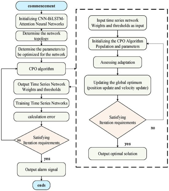
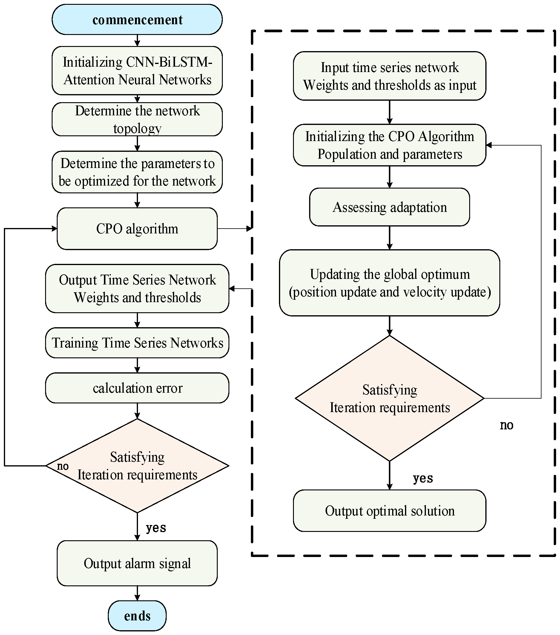
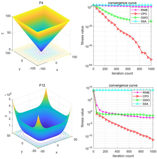
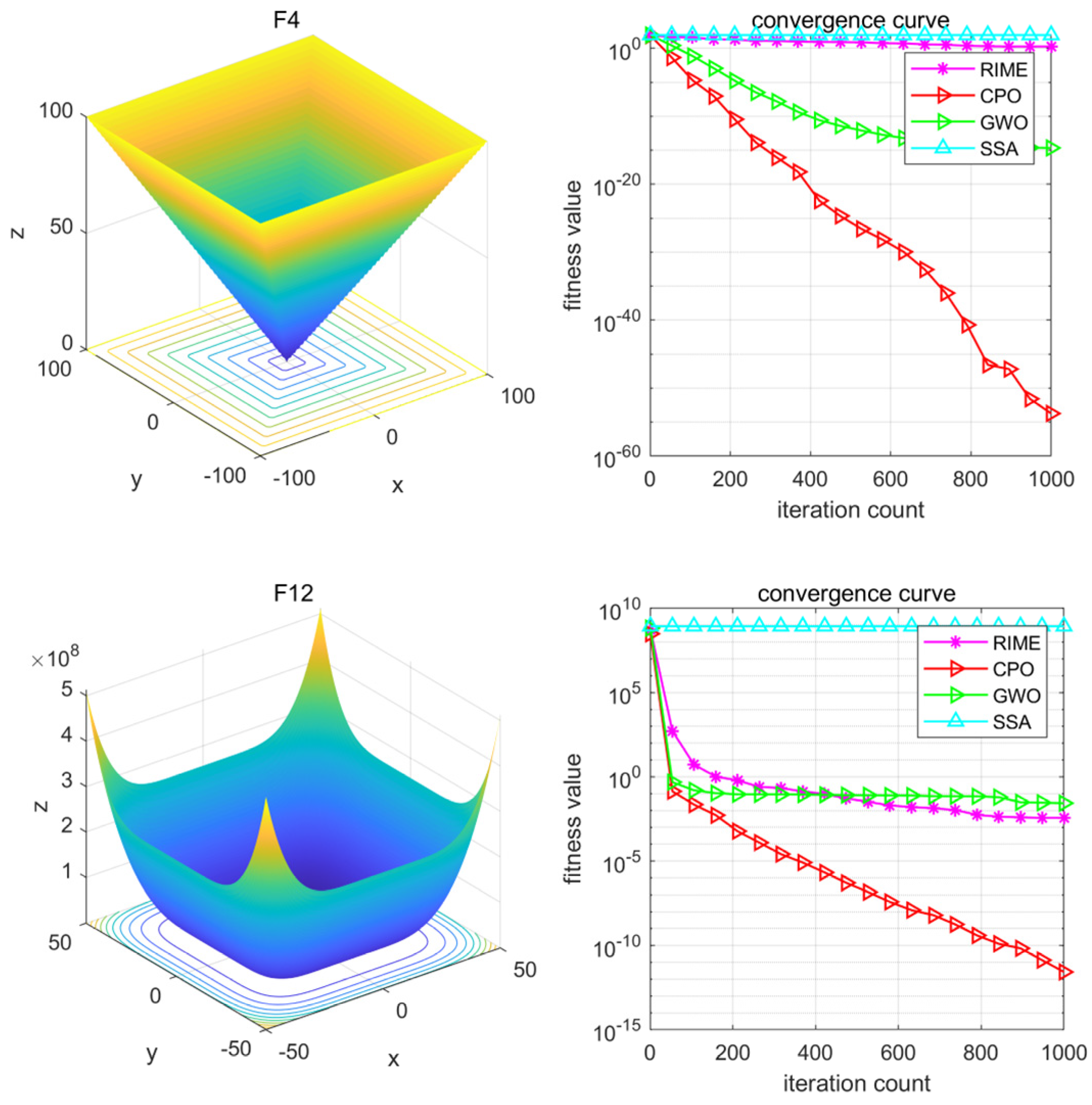
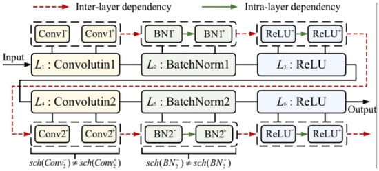
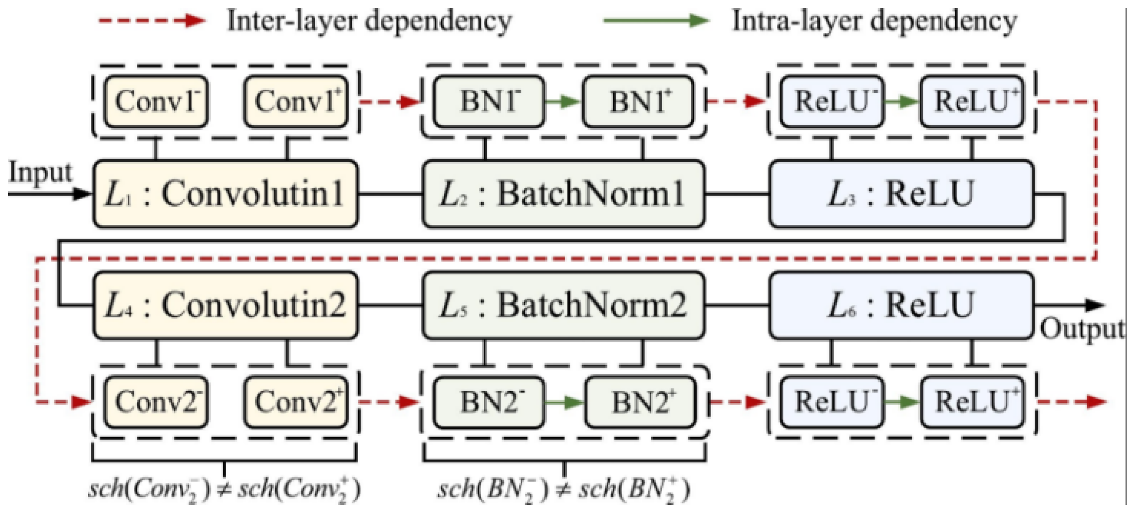
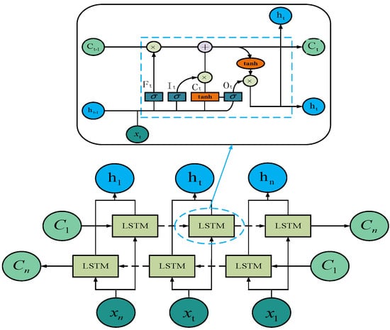
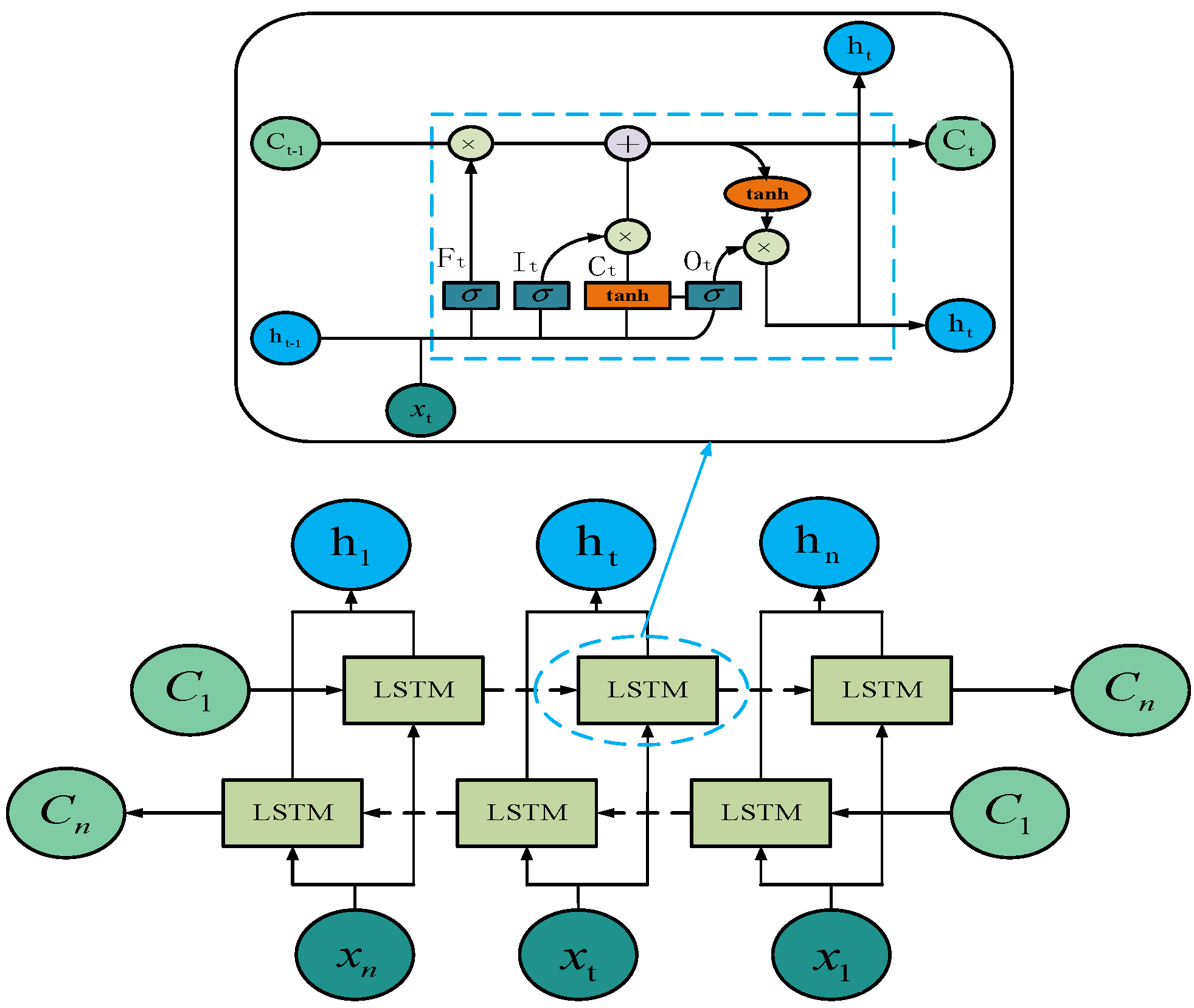
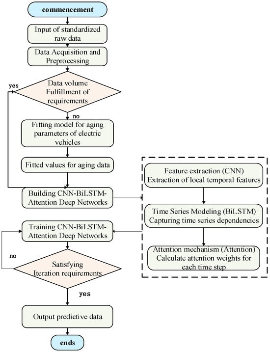
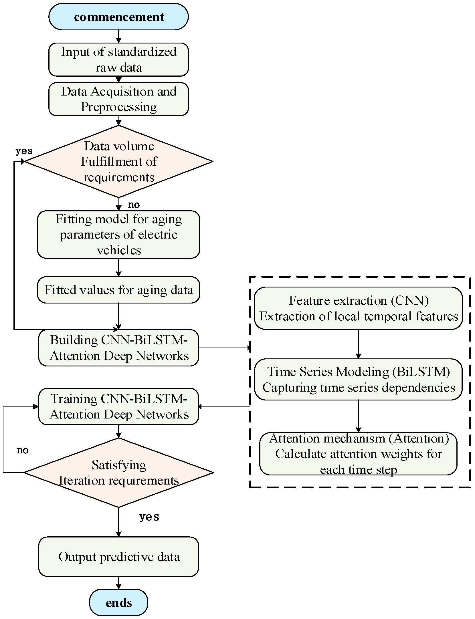
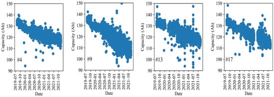
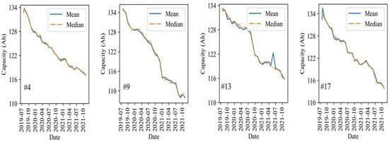
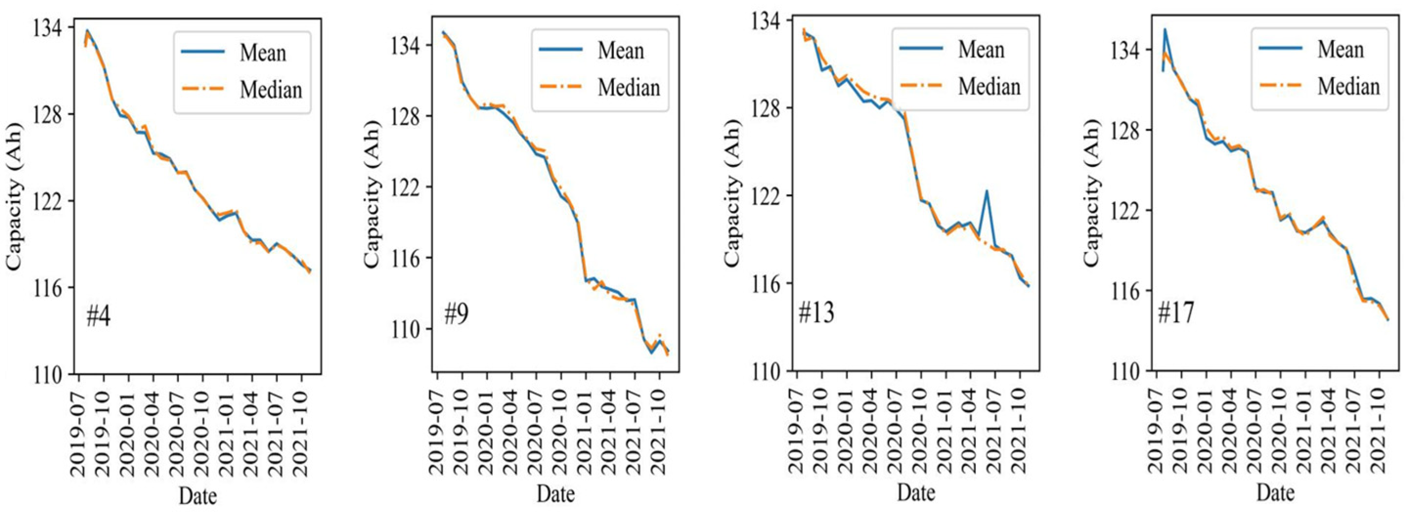
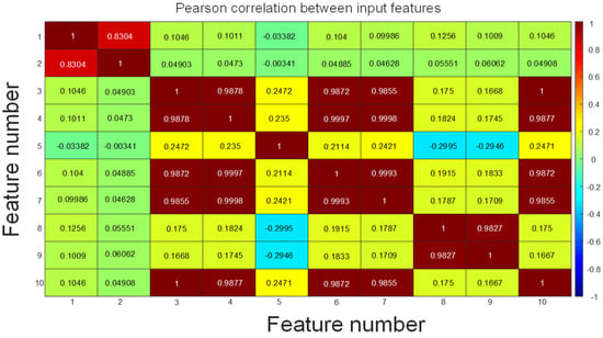
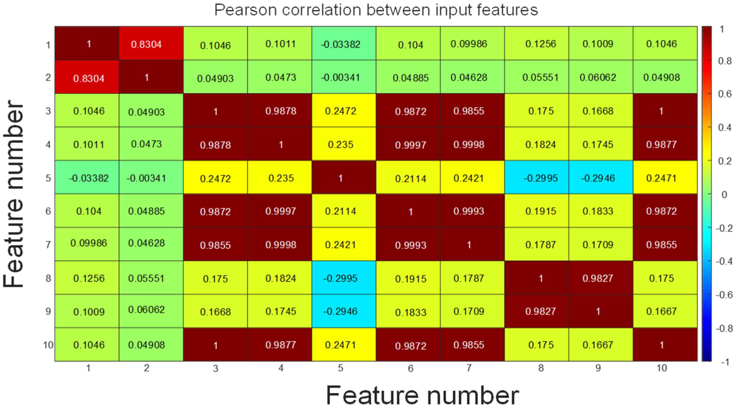
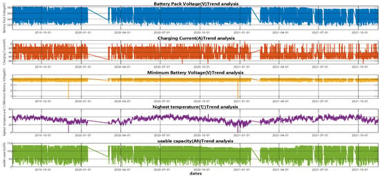
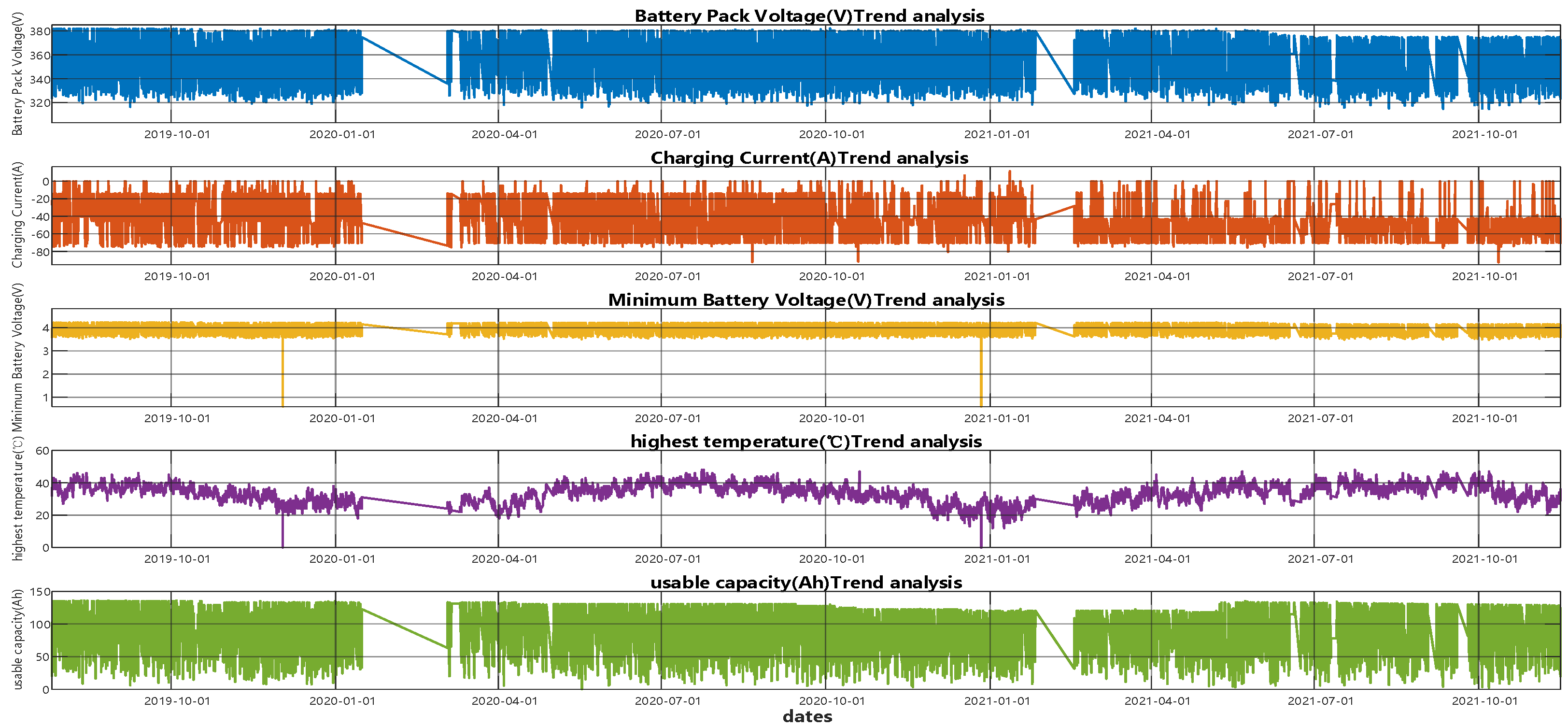
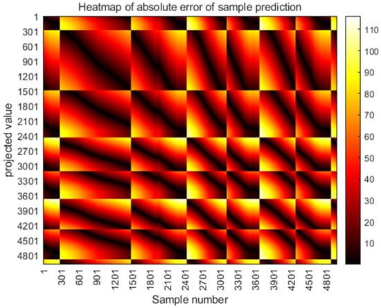
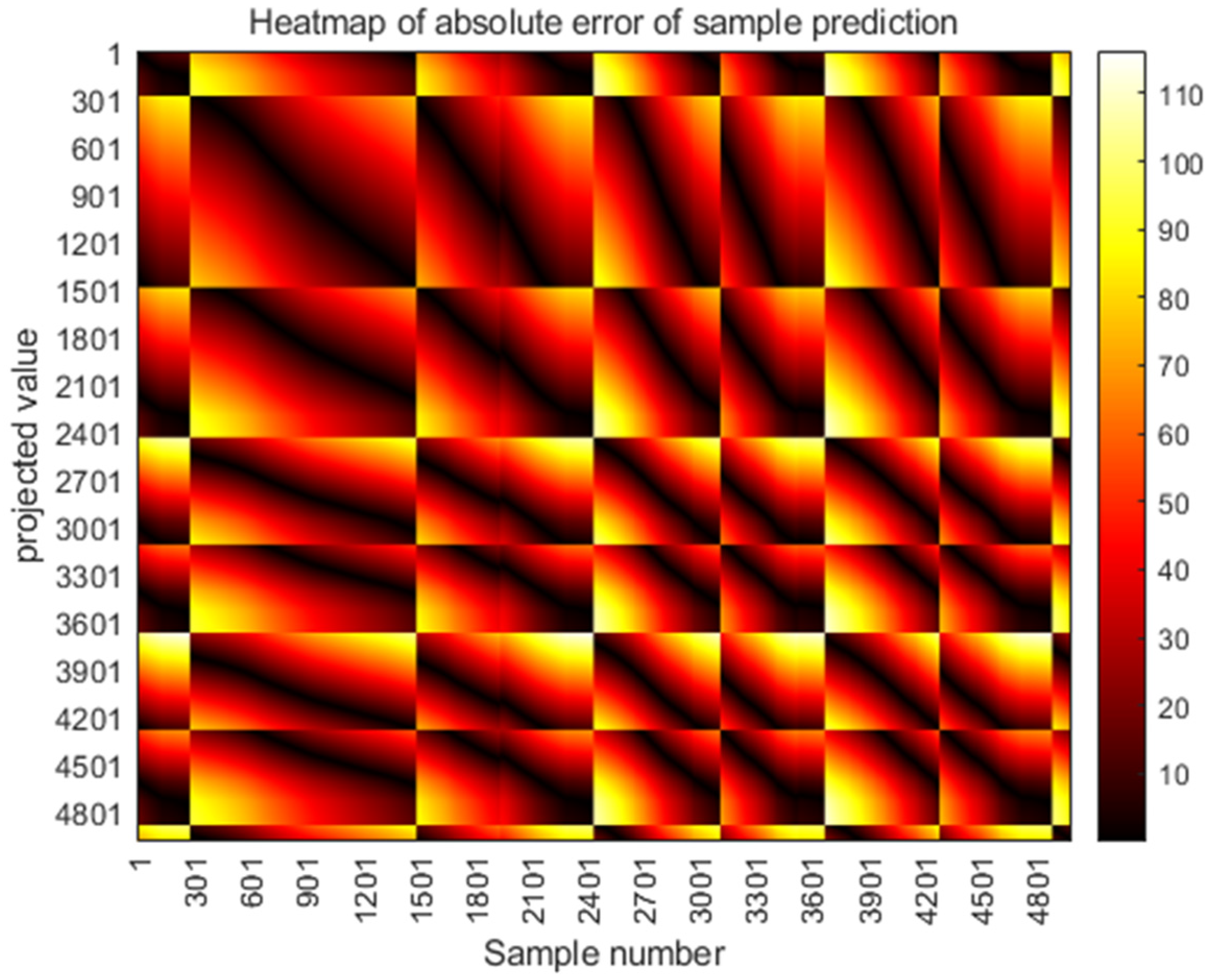
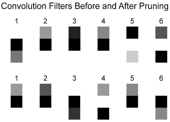
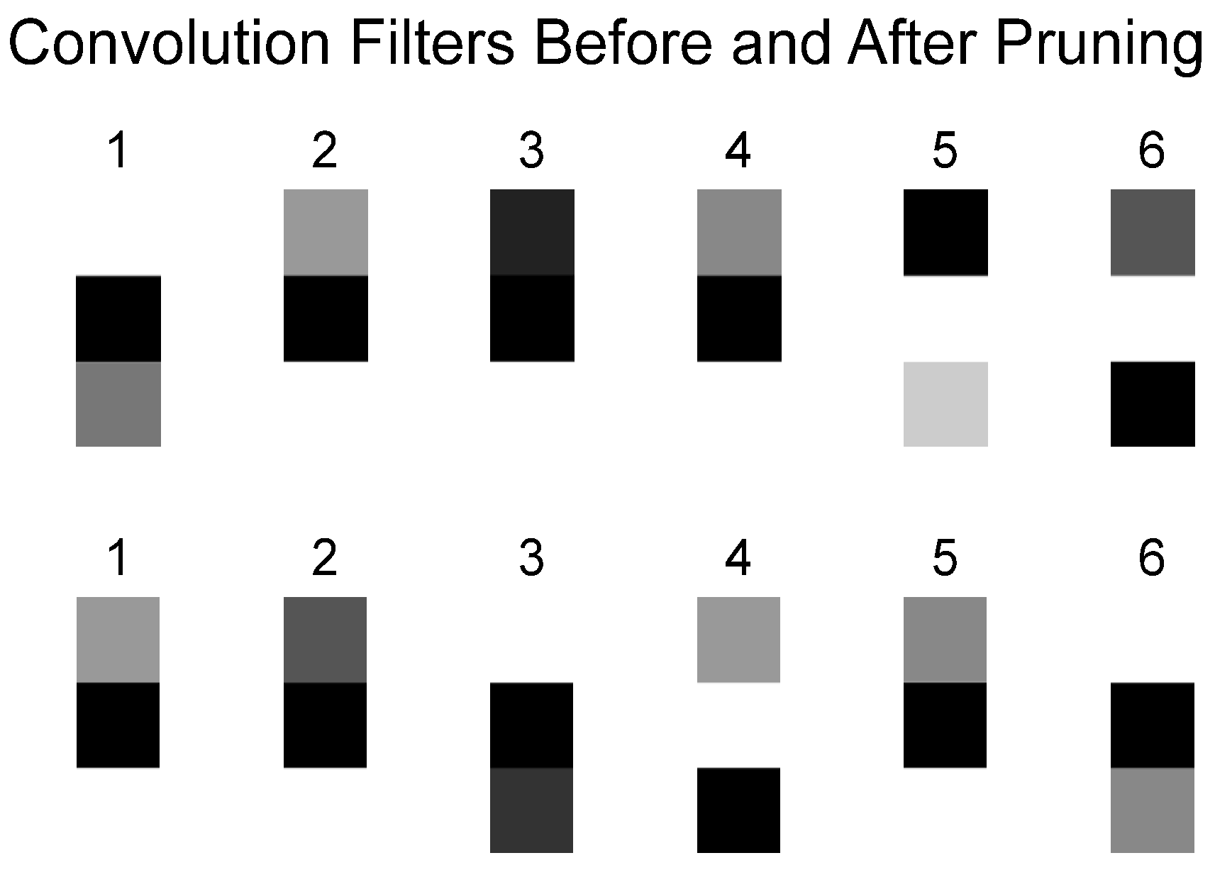
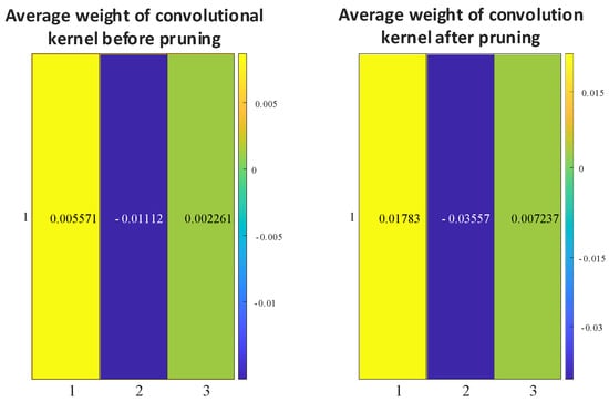
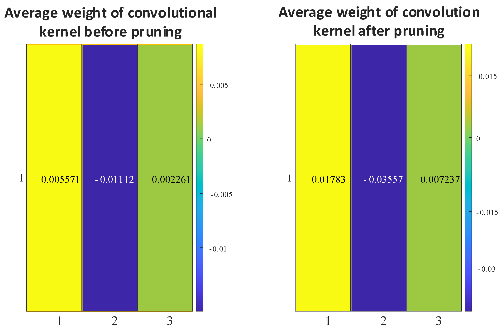
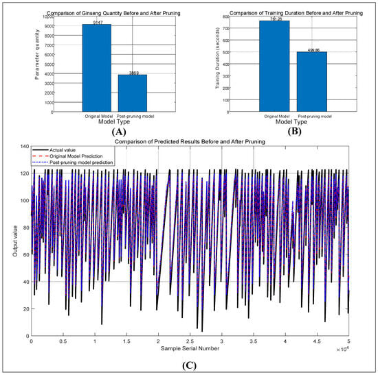
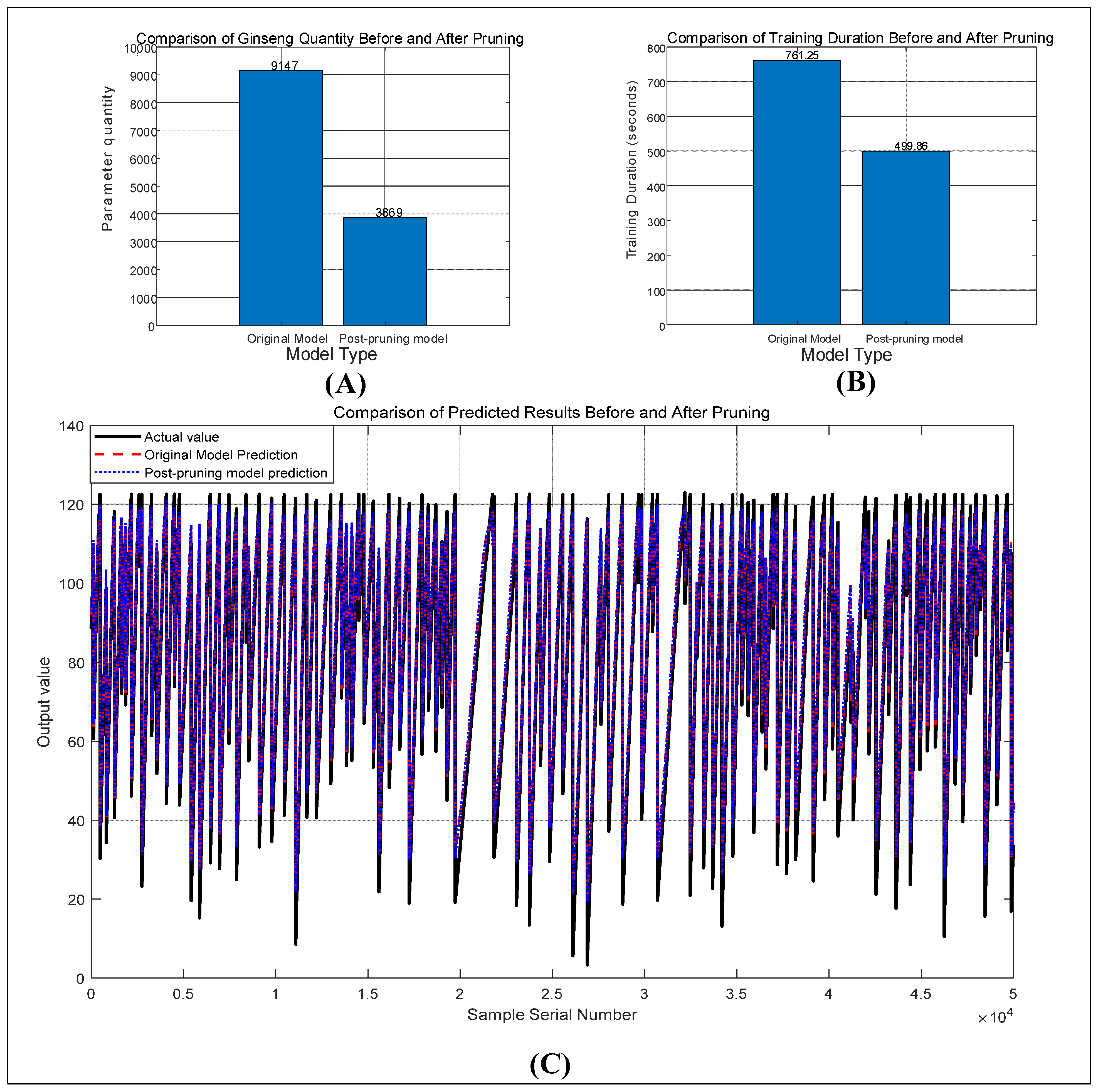
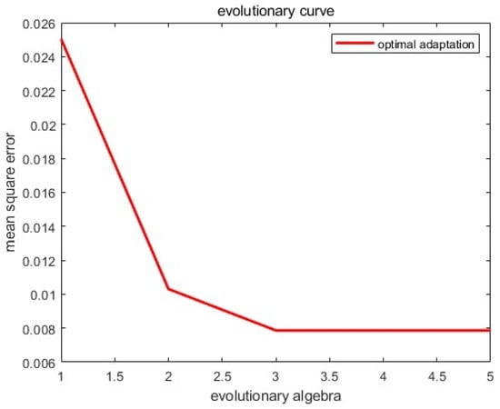
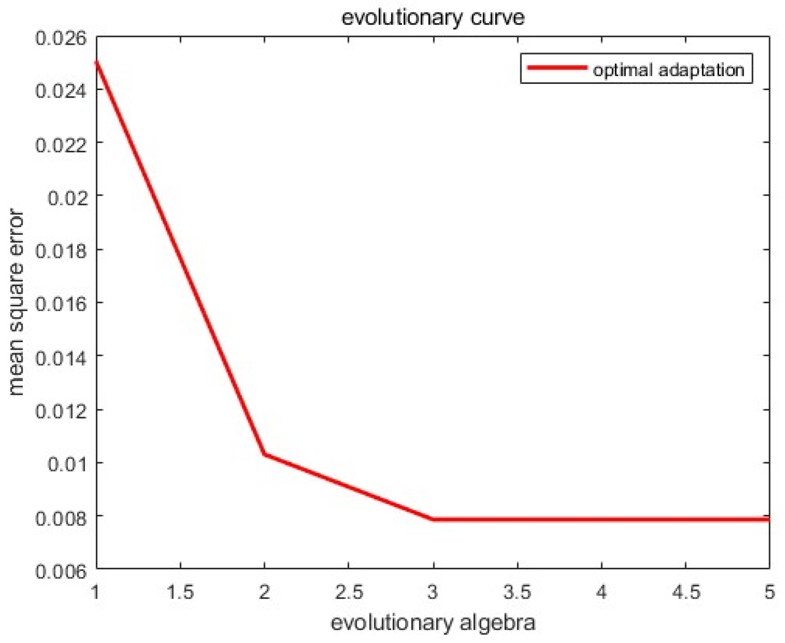
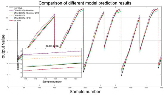
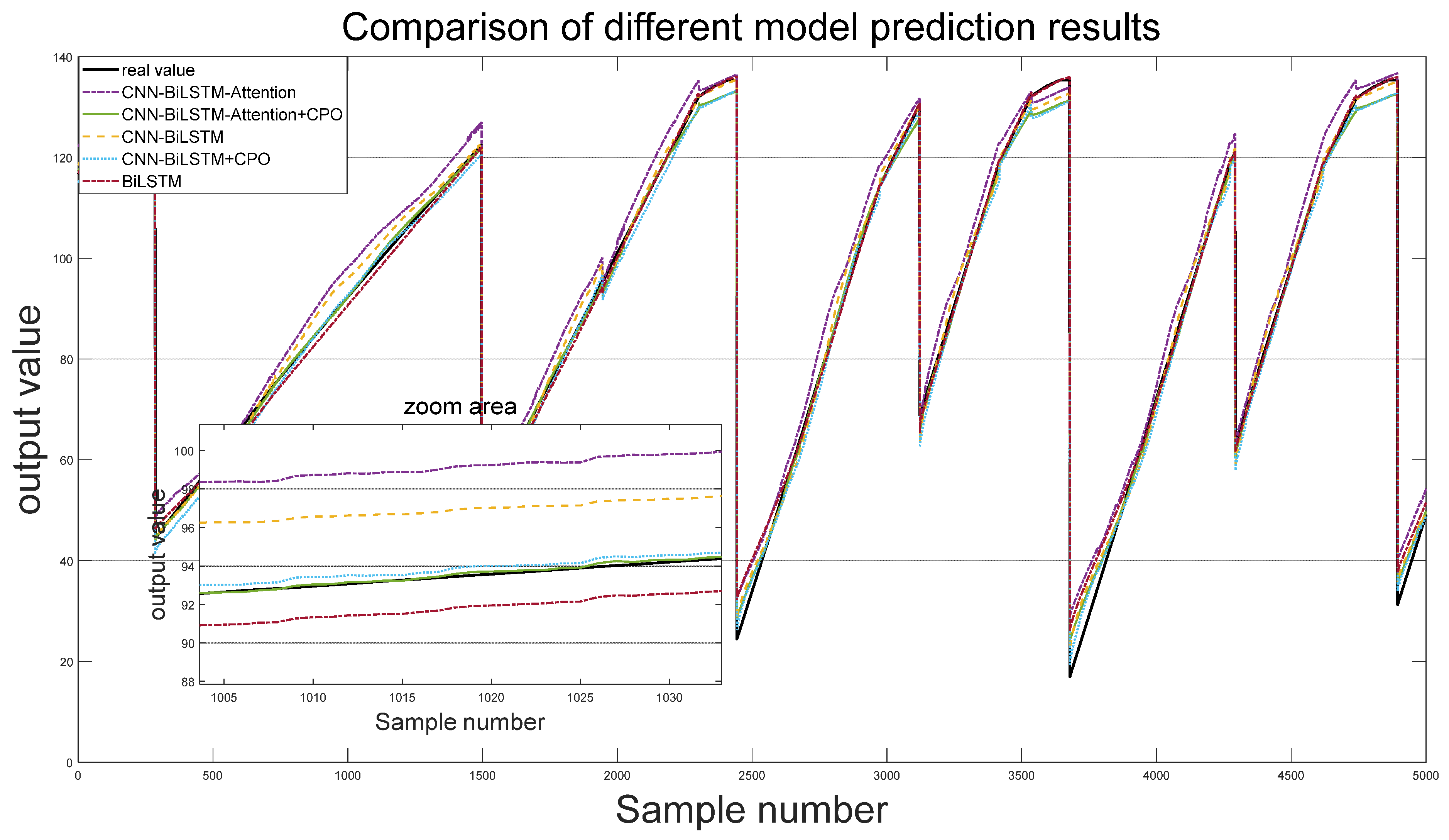
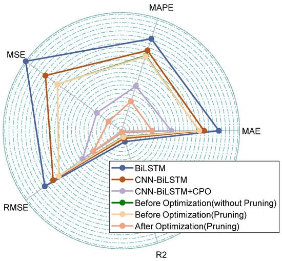
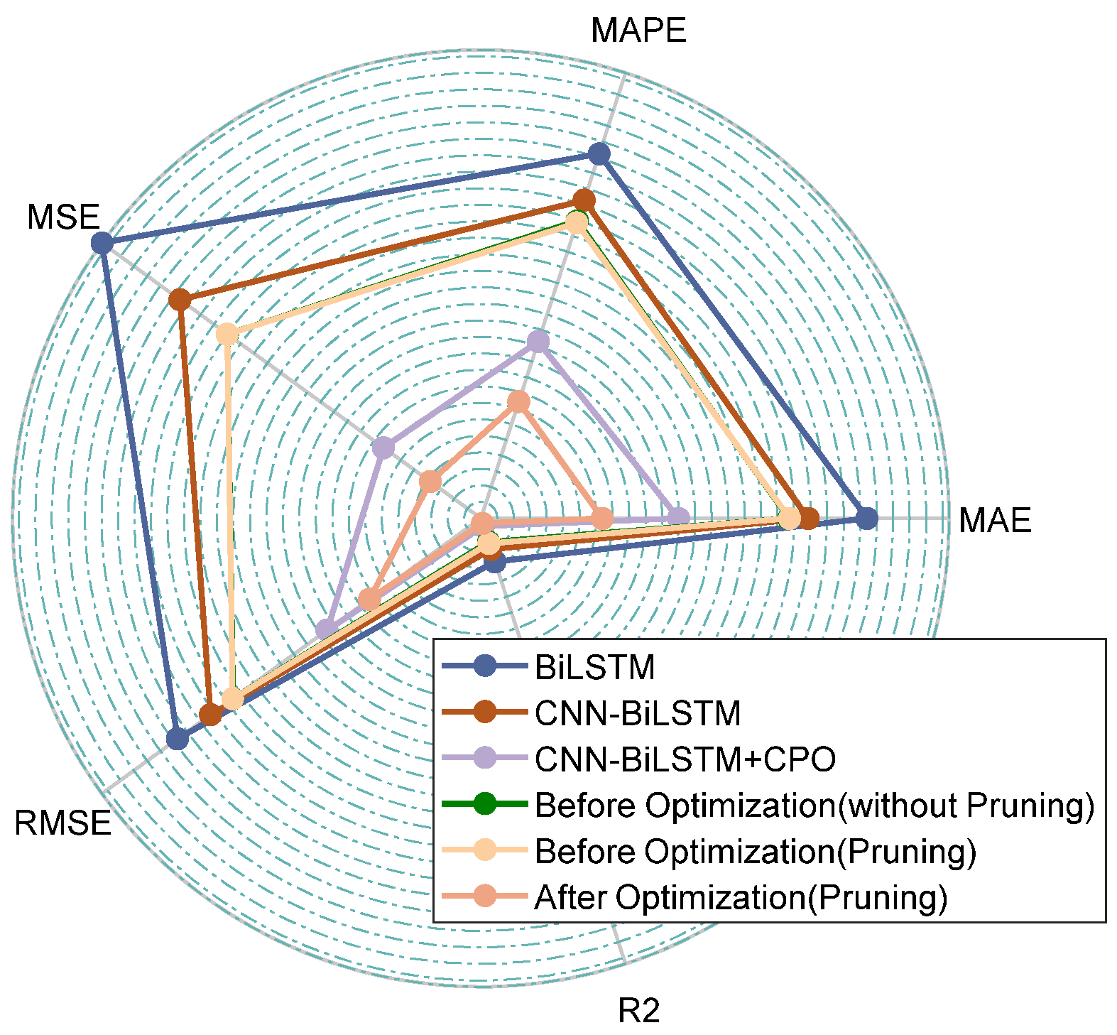
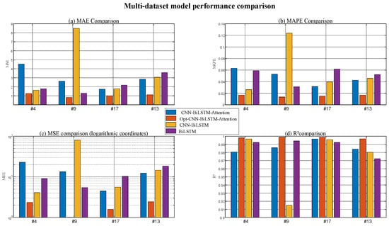
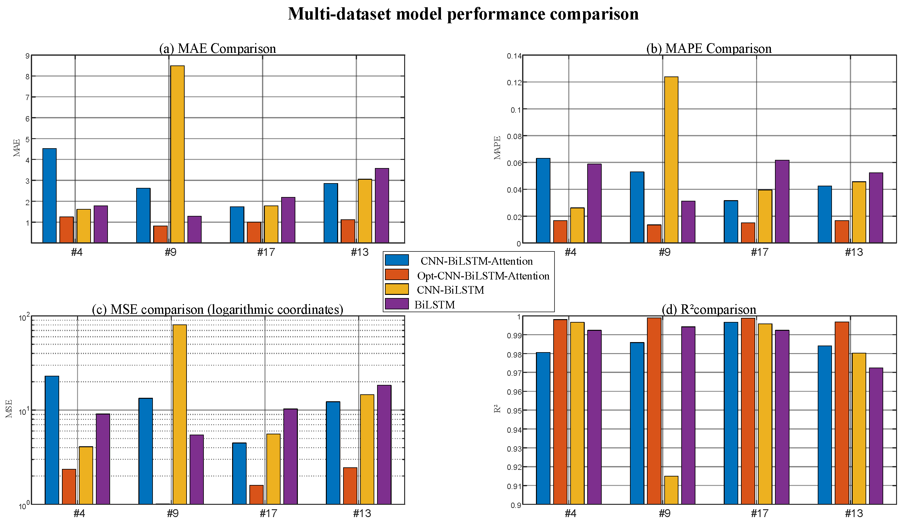
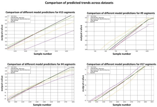
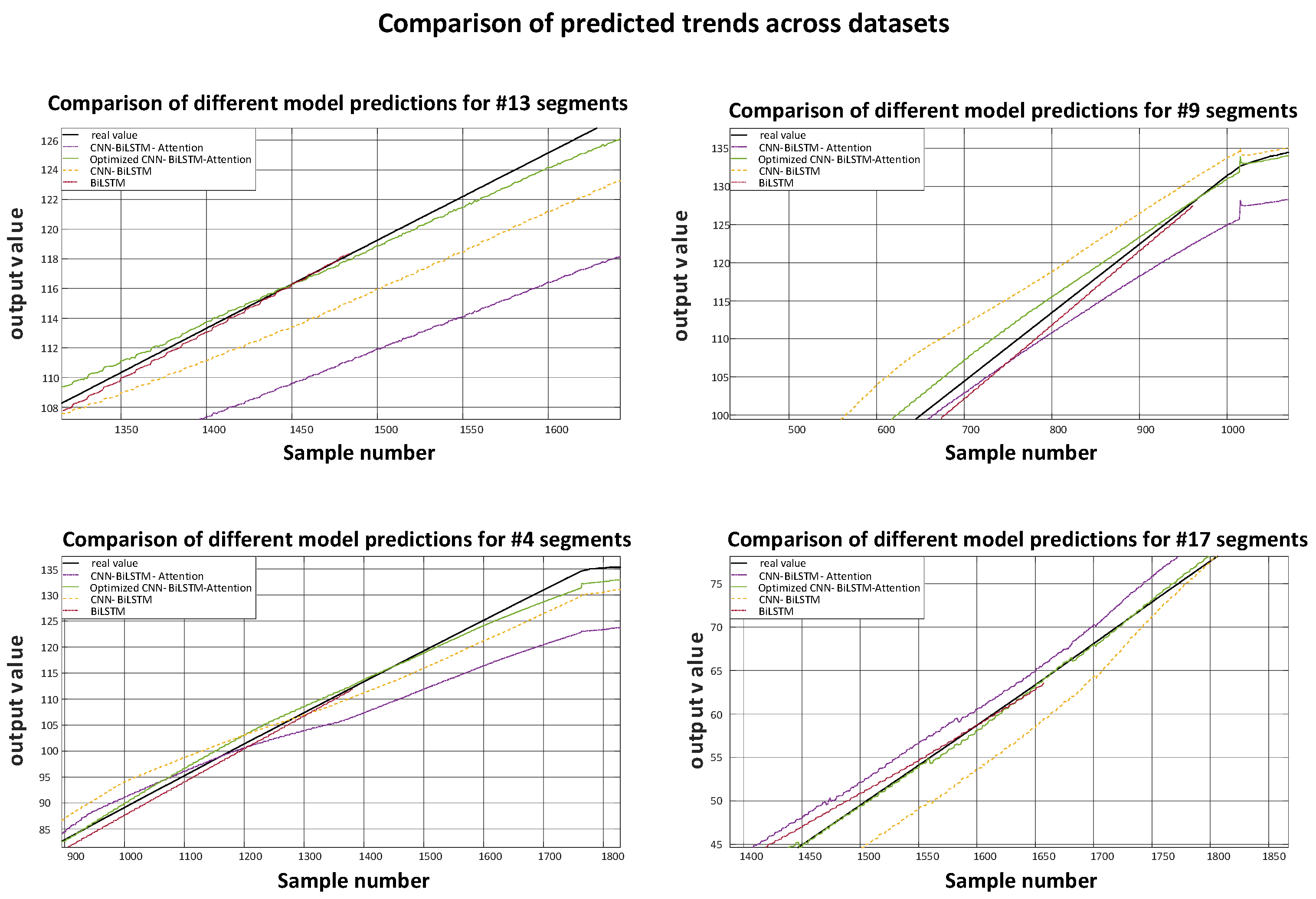

Disclaimer/Publisher’s Note: The statements, opinions and data contained in all publications are solely those of the individual author(s) and contributor(s) and not of MDPI and/or the editor(s). MDPI and/or the editor(s) disclaim responsibility for any injury to people or property resulting from any ideas, methods, instructions or products referred to in the content. |
© 2026 by the authors. Licensee MDPI, Basel, Switzerland. This article is an open access article distributed under the terms and conditions of the Creative Commons Attribution (CC BY) license.