Dynamic Graph-Based Cross-City Traffic Prediction Framework with Domain-Level Feature Alignment and Node-Level Personalization

Abstract

The deployment of intelligent transportation systems (ITS) in emerging urban areas faces significant challenges due to the scarcity of historical data. Knowledge transfer across cities has shown exciting potential in addressing this issue, yet existing methods typically rely on predefined or static graphs, neglecting dynamic spatio-temporal relationships. Moreover, they handle data distribution discrepancies solely at the domain or node level, neglecting the multi-granularity heterogeneity inherent in urban data distributions. In this paper, we propose a Dynamic Graph-based Cross-city Traffic Prediction Framework (DGCTF), which introduces an adaptive graph structure learner to capture dynamic spatio-temporal relationships and complex interdependencies among cities. Besides, DGCTF addresses data discrepancy issue at multiple granularities. At the domain-level, DGCTF reduces data distribution differences across cities through a cross-domain feature alignment training method with Cross-Domain Feature Alignment Loss (CDFAL). At the node-level, DGCTF enables fine-grained adaptation via a Residual-enhanced GRU with Node-level Parameter-Matching strategy (RGRU-NodePM) by generating node-specific parameters to model node correlations across cities. Experimental results on multiple real-world datasets demonstrate that DGCTF significantly outperforms state-of-the-art methods in both short-term and long-term predictions. Notably, in several cross-city prediction tasks, DGCTF outperforms the second-best methods by up to 5.78% in MAE, 2.39% in RMSE, and 8.65% in MAPE.

1. Introduction

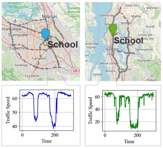
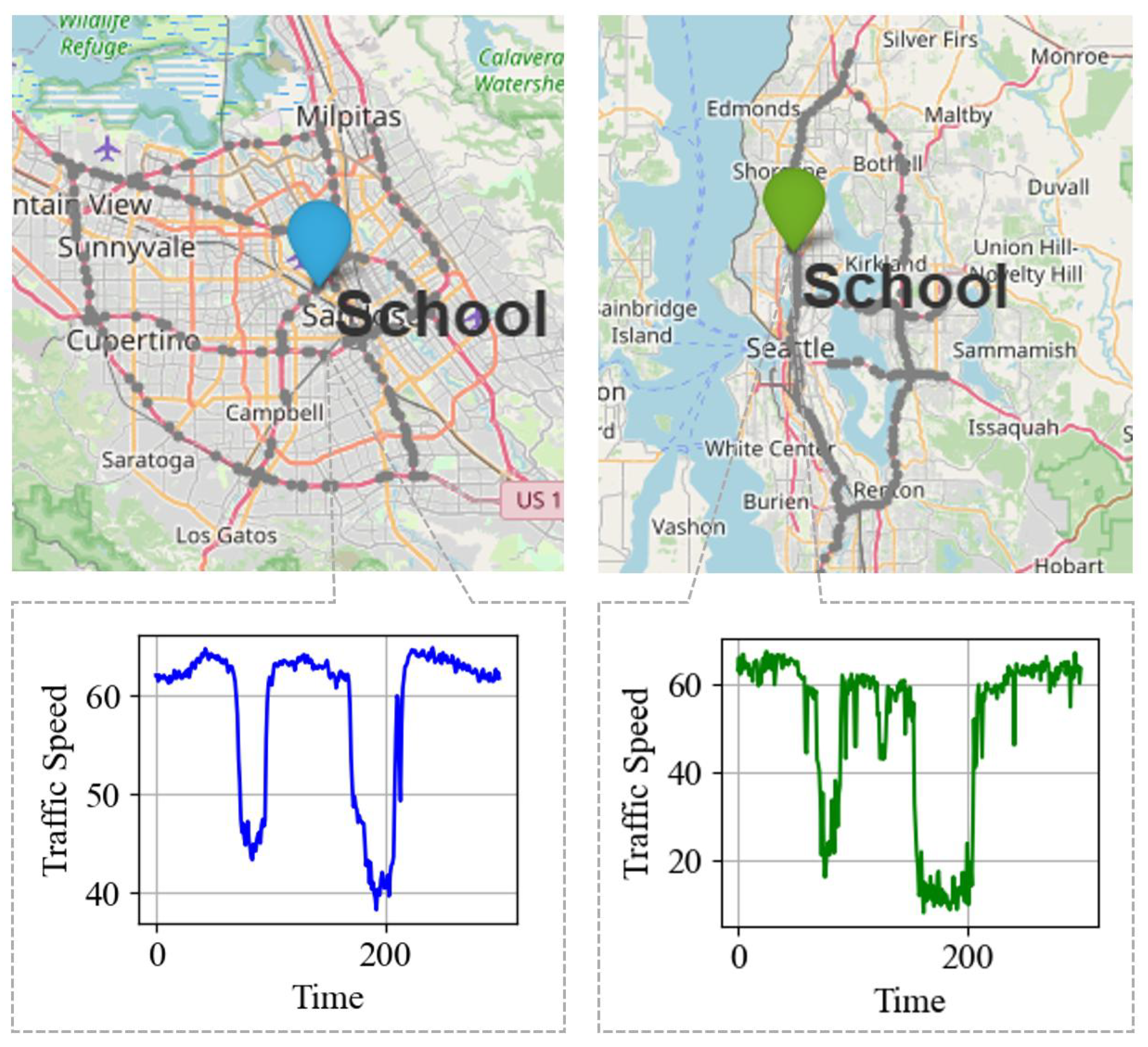
Traffic prediction is a key service in intelligent transportation systems (ITS). Detailed and timely traffic prediction not only helps city policy-makers in decision-making and resource allocation, but also assists urban residents in travel planning. Furthermore, precise traffic prediction is essential for V2X-enabled cooperative control to effectively mitigate aperiodic congestion in mixed traffic environments [1]. In recent years, deep learning models such as convolutional neural networks (CNNs) [2] and graph neural networks (GNNs) [3], with their powerful computational capabilities that surpass traditional methods, have been widely applied to traffic tasks. However, the success of these deep learning models is heavily dependent on large-scale traffic data, which is not always available in real-world scenarios, especially when predicting emerging regions that lack historical data. Notably, cities tend to share similar underlying patterns in traffic dynamics. As an example shown in Figure 1, functionally similar areas across cities, e.g., schools, exhibit comparable traffic patterns, suggesting that the fundamental dynamics of traffic can be generalized across cities. In this context, transfer learning offers a possible solution to the problem of data scarcity by transferring knowledge from data-rich cities to data-scarce cities [4], thereby reducing the burden of data collection and improving the efficiency of smart city development.

Figure 1. The illustration of spatio-temporal patterns of San Francisco (left) and Seattle (right).

In transfer learning research, some methods divide cities into grids with fixed sizes and spatial relationships to capture regional spatio-temporal characteristics and employ sophisticated techniques to understand the relationships between the source and target domains [5,6,7]. However, grid-based data are not suitable for describing topology structures with irregular and flexible node connections. With the development of GNNs, some researchers [4,8,9] propose graph-based methods using meta-learning and domain adaptation to transfer knowledge. These works rely on pre-defined graphs that are manually designed and may include noise, missing data, and biases [10], which increase the risk of negative transfer between the source and target cities. Recognizing these limitations, some researchers employ graph learners to acquire learnable static graphs and utilize regularization techniques with joint training of the source and target cities to transfer knowledge [10]. Although these methods have improved cross-city traffic prediction to some extent, transfer learning methods used for traffic prediction still face the following two challenges.

(1) Capturing dynamic spatio-temporal dependencies in transfer learning: Due to factors such as weather, pedestrian density, traffic control, and traffic accidents, the spatial dependencies in traffic networks change dynamically over time, with cities exhibiting periodic spatio-temporal patterns. Previous transfer learning methods use predefined graphs [4,8,9] or adaptive static graphs [10] for knowledge transfer as they assume that the data are static and identically distributed. However, static graph structures are incapable of encapsulating the inherent complex dynamic spatial dependencies in cities characterized by intricate and interwoven spatial attributes and temporal patterns. Recently, substantial studies have been conducted on dynamic graphs [11,12,13], which generate task-specific dynamic graphs. However, these methods are typically designed for single-city scenarios and involve extensive parameters, limiting their applicability in transfer learning. Therefore, exploring flexible, dynamic, and transferable graph structure learner to capture similar spatio-temporal patterns between cities or nodes and improve cross-city prediction performance remains an area for further research.

(2) Exploring data discrepancy at both domain and node level: Due to differences in infrastructure, socio-economic factors, population density, and local policies, the domain-level traffic data distribution varies significantly across cities. Existing methods such as TransGTR [10] and CityTrans [4] reduce spatio-temporal feature differences between source and target cities through adversarial learning or metric learning, and share model parameters between cities. However, simply reducing data distribution differences at the domain-level risks overlooking unique node-level features in the target domain, especially for functional nodes such as schools or hospitals, which exhibit distinct temporal patterns. There are methods that focus on transferring node-specific knowledge. TPB [14], MTPB [15], NodeTrans [16] and ST-GFSL [8] transfer node-level knowledge through clustering or parameter sharing. However, focusing solely on the transfer of node-level knowledge overlooks global data distribution differences, obscuring an understanding of the overall traffic dynamics. Therefore, a reasonable strategy that simultaneously reduces domain-level data distribution differences and incorporates node-level adaptive personalization remains an imperative area for further investigation.

In this paper, our goal is to achieve cross-city knowledge transfer based on dynamic graphs for the target city with limited data and to handle data distribution differences at both domain-level and node-level granularities. We propose a Dynamic Graph-based Cross-city Traffic Prediction Framework (DGCTF), which pioneers the integration of dynamic graphs into multi-source transfer learning, capturing time-varying spatial features through a dynamic adaptive graph convolution network. In addition, Cross-Domain Feature Alignment Loss (CDFAL) is designed to make graph structure learner transferable by ensuring that the features the learner extracts follow a similar distribution among cities at domain-level. In addition, a Residual-enhanced Gated Recurrent Unit with Node-level Parameter-Matching strategy (RGRU-NodePM) is designed to achieve node-level knowledge transfer by establishing associations between nodes across cities and generating node-specific parameters through the Node-Aware Parameter Generator (NAPG). We manage data discrepancies at both domain-level and node-level granularities by reducing domain-level data distribution differences and enabling node-level personalized adaptation. This design allows the model to effectively address both inter-city and intra-city differences in cross-domain traffic prediction. The main contributions of this paper are summarized as follows:

• A dynamic adaptive graph convolution network with adaptive graph structure learner and multi-graph fusion convolutional layer is proposed to extract the dynamic features across cities.
• A residual-enhanced gated recurrent unit with node-level parameter-matching strategy (RGRU-NodePM) is designed to transfer node-level knowledge by customizing node-specific model parameters through NAPG.
• A cross-domain feature alignment loss (CDFAL) is designed to reduce domain-level data distribution differences in multi-source scenarios and make graph structure learner transferable.
• Extensive experiments on seven public datasets verify the effectiveness of our method. Compared to other state-of-the-art models, our method significantly and consistently improves prediction accuracy for both long-term and short-term forecasts.

The rest of the paper is organized as follows: Section 2 briefly reviews related work. Section 3 presents the definition of the research problem in this study. The general framework of our DGCTF and the specific solutions are detailed in Section 4. In Section 5, we design several experiments to evaluate our model. Our work and directions for future research are summarized in Section 6.

2. Related Work

2.1. Graph Structure Learning

Pre-defined graph: Traffic networks exhibit a strong graph structure, making them well-suited for graph convolution [17], which excels in capturing complex spatial relationships. STGCN [18], TGCN [19] and DCRNN [20] are representative works that use pre-defined explicit graph structures to capture spatial features of nodes. However, pre-defined graph structures cannot handle the dynamic relationships between nodes.

Learnable static graph: Some researchers attempt using learnable static graphs to capture the task-relevant node association. For example, Graph WaveNet [21] and MTGNN [22] construct adaptive adjacency matrices using node embeddings and external information to capture hidden spatial dependencies. AGCRN [23] introduces adaptive modules to capture node-specific patterns, while ASTGCRN [24] enhances it with an attention mechanism. STGODE [25] employs dynamic time warping to build a semantic adjacency matrix, addressing the limitations of predefined graphs in capturing similar spatio-temporal patterns of distant nodes. Recently, TransGTR [10] applies a learnable static graph to transfer learning by training the structure generator via a temporal decoupled regularization. Experimental results show that effective graph structure learning better uncovers latent spatio-temporal relationships and facilitates knowledge transfer more effectively than predefined graphs. However, traffic data exhibit strong dynamic spatio-temporal correlations, which cannot be expressed by static graphs.

Dynamic graph: Recognizing that the static graph is not capable of representing the temporal variations in node connectivity, some studies work on building dynamic graphs. ST-GDN [26] utilizes multi-resolution transition information and local-global regional dependencies for prediction. DSTAGNN [27] learns the dynamic spatial-temporal awareness graph through the cosine distance and an improved self-attention mechanism. AGFCRN [11] adaptively learns dynamic and static graphs and utilizes graph fusion convolution to integrate static and dynamic features. DyHSL [28] proposes a dynamic hypergraph structure learning block to model dynamic non-pairwise relationships by constructing hypergraphs. DMGAN [29] introduces multi-hop neighbors when calculating dynamic spatial dependencies, which expands the receptive field of the target node and adaptively captures changes in network connectivity. DDGCRN [30] designs a spatio-temporal embedding generator that fully considers periodic changes in the traffic network to construct a dynamic graph that includes temporal periodicity information. Previous studies suggest that dynamic graph learning effectively captures the evolving spatio-temporal interactions in traffic networks.

While the aforementioned approaches have demonstrated impressive performance in traffic prediction, they are typically tailored to individual cities and are dependent on substantial quantities of parameters and training samples, making them prone to overfitting when deployed in cross-domain scenarios with limited data [10]. Therefore, in this paper, we are committed to investigating the means of integrating dynamic graphs into cross-city transfer learning to improve the prediction accuracy for the target city with scarce data.

2.2. Transfer Learning for Traffic Forecasting

Due to high data collection costs and stringent privacy regulations, data scarcity has become a common challenge for data-driven methods. Transfer learning has been applied to alleviate the problem of data scarcity in prediction by transferring knowledge from source cities with rich data to target cities with scarce data. Early approaches such as RegionTrans [6] and MetaST [7] transfer spatial or spatio-temporal features via region matching or meta-learning. Later works like ARG-STNet [31] and CrossTReS [5] introduced attention and weighting mechanisms to enhance transfer effectiveness.

However, these methods ignore data distribution differences between cities, leading to negative transfer when there is a significant data distribution difference between the source and the target cities. Methods addressing data distribution differences can generally be categorized into two types: domain-level approaches and node-level approaches.

Domain-level methods: They focus on the overall characteristics of a city. For example, ST-DAAN [32] utilizes Maximum Mean Discrepancy (MMD) to reduce the data distribution differences between the source and target domains, while STAN [33] employs adversarial learning to obtain domain-invariant spatio-temporal features. However, these methods are designed for grid data and are not compatible with graph-structured spatio-temporal data. With the development of GNNs, several models based on graph data have emerged, such as DASTNET [9], CityTrans [4], and Ada-STGCN [34], which achieve knowledge transfer through adversarial learning and domain adaptation techniques. TransGTR [10] combines graph structure learning with metric learning and proposes the use of a learnable adaptive static graph structure for traffic prediction. STGP [35] introduces domain prompting to dynamically adapt the target domain data. Domain-level methods merely transfer graph embeddings or features of source cities as a whole and reduce the overall distribution differences between different cities, ignoring heterogeneity and correlations among nodes.

Node-level methods: They focus on the specific characteristics of nodes, capturing interactions among nodes. For instance, NodeTrans [16] clusters spatio-temporal patterns of nodes in the source domain and selectively transfers the parameters to the target city. ST-GFSL [8] generates non-shared feature extractor parameters using node-specific feature, essentially proposing a parameter initialization strategy for transfer learning. TPB [14] and MTPB [15] employ clustering techniques to construct a traffic pattern library in the source cities and generate node-level meta-knowledge by querying the traffic pattern library to guide downstream predictions. However, these methods transmit node-level knowledge through parameter sharing or parameter matching, overlooking global feature differences and data distribution variations, which can hinder effective knowledge transfer when data distributions vary significantly between different cities [36].

Research that simultaneously considers domain-level and node-level data distribution differences for traffic prediction transfer learning is relatively rare. DGCN [36] captures node-level correlations by constructing cross-city node adjacency relationships and reduces domain-level data distribution differences by using domain adversarial learning. However, the joint training strategy used in this method limits its applicability to scenarios with multiple source cities.

In this paper, we propose DGCTF, a novel cross-city traffic prediction framework which introduces the graph structure learner to construct dynamic graphs that effectively capture evolving spatio-temporal relationships. Unlike existing approaches that learn the dynamic graph structures in a single city, our method focuses on developing dynamic graph structures that encode transferable knowledge across cities. Meanwhile, instead of merely incorporating domain-level global information or node-level local details, we address data distribution discrepancies at both domain-level and node-level granularities to ensure both global consistency and local adaptability.

3. Preliminary

Definition 1

(Traffic Spatio-Temporal Graph). A traffic spatio-temporal graph can be denoted as $\mathcal{G}=(V,\mathcal{E},\mathit{A},\mathit{X})$ [8]. V is the set of nodes and $N=\left|V\right|$ is the number of nodes. $\mathcal{E}$ is the set of edges, and each edge can be denoted as $e_{ij}=(v_i,v_j)$. $\mathit{A}\in {\mathbb{R}}^{N\times N}$ is the adjacency matrix of $\mathcal{G}$, where $a_{ij}=1$ indicates that there is an edge between $v_i$ and $v_j$. $\mathit{X}\in {\mathbb{R}}^{N\times T\times C}$ is the node feature matrix, referring to the message that passes through the graph. We take the node feature at time t as a graph signal ${\mathit{X}}_t\in {\mathbb{R}}^{N\times C}$, where C is the dimension of node feature.

Definition 2

(Multi-source Cross-city Few-Shot Traffic Forecasting). Given M source cities ${\mathcal{G}}^{\mathcal{S}}=\{{\mathcal{G}}^{{\mathcal{S}}_1},\cdots ,{\mathcal{G}}^{{\mathcal{S}}_M}\}$ with rich data and a target city ${\mathcal{G}}^{\mathcal{T}}$ with only limited data, the goal of multi-source cross-city few-shot traffic forecasting is to learn a model based on the available data of both ${\mathcal{G}}^{\mathcal{S}}$ and ${\mathcal{G}}^{\mathcal{T}}$ to perform traffic forecasting on future data of ${\mathcal{G}}^{\mathcal{T}}$ [8].

Definition 3

(Transferable Structure Learning for Traffic Forecasting). In the pre-training stage, given multiple source cities and a target city with graph-based traffic data ${\mathcal{G}}^{{\mathcal{S}}_i}=\left(V^{{\mathcal{S}}_i},{\mathcal{E}}^{{\mathcal{S}}_i},{\mathit{A}}^{{\mathcal{S}}_i},{\mathit{X}}^{{\mathcal{S}}_i}\right)$ and ${\mathcal{G}}^{\mathcal{T}}=\left(V^{\mathcal{T}},{\mathcal{E}}^{\mathcal{T}},{\mathit{A}}^{\mathcal{T}},{\mathit{X}}^{\mathcal{T}}\right)$, for task sampling, ${\mathit{X}}^{{\mathcal{S}}_i}\in {\mathbb{R}}^{N_{{\mathcal{S}}_i}\times T_{{\mathcal{S}}_i}\times C}$, ${\mathit{X}}^{\mathcal{T}}\in {\mathbb{R}}^{N_{\mathcal{T}}\times T_{\mathcal{T}}\times C}$, where $T_{\mathcal{T}}\ll T_{{\mathcal{S}}_i}$, we aim to learn a well-initialized graph structure learner $f_{\varphi }$ and a forecasting model $f_{\theta }$. Suppose that we have T historical spatio-temporal graph signals and we want to predict future P graph signals:

$${\mathit{X}}^{S_i},{\mathit{X}}^T\stackrel{f_{\varphi }(·;\varphi )}{\to }{\mathit{A}}^{S_i}\left(\varphi \right),{\mathit{A}}^T\left(\varphi \right),$$

(1)

$$\begin{array}{c}\hfill \begin{array}{c}\hfill \left[{\mathit{X}}_{t-T+1:t}^{S_i};{\mathit{X}}_{t-T+1:t}^T;{\mathit{A}}^{S_i}\left(\varphi \right);{\mathit{A}}^T\left(\varphi \right);{\epsilon }^{S_i};{\epsilon }^T\right]\\ \hfill \stackrel{f_{\theta }(·;\theta )}{\to }\left[{\mathit{X}}_{t+1:t+P}^{S_i};{\mathit{X}}_{t+1:t+P}^T\right],\end{array}\end{array}$$

(2)

where ϕ and θ denote the learned function parameters.

In the fine-tuning stage, the same function initialized with parameters ϕ, θ shared from the pretrained function is fine-tuned to predict graph signals on the target road network:

$${\mathit{X}}^T\stackrel{f_{\varphi }(·;{\varphi }_{*}\left(\varphi \right))}{\to }{\mathit{A}}^T\left(\varphi \right),$$

(3)

$$[{\mathit{X}}_{t-T+1:t}^T;{\mathit{A}}^T\left(\varphi \right),{\epsilon }^T]\stackrel{f_{\theta }(·;{\theta }_{*}\left(\theta \right))}{\to }\left[{\mathit{X}}_{t+1:t+P}^T\right],$$

(4)

where ${\varphi }_{*}\left(\varphi \right)$ and ${\theta }_{*}\left(\theta \right)$ denote the function parameters adjusted from ϕ and θ to fit the target domain.

4. Methodology

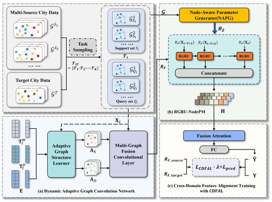
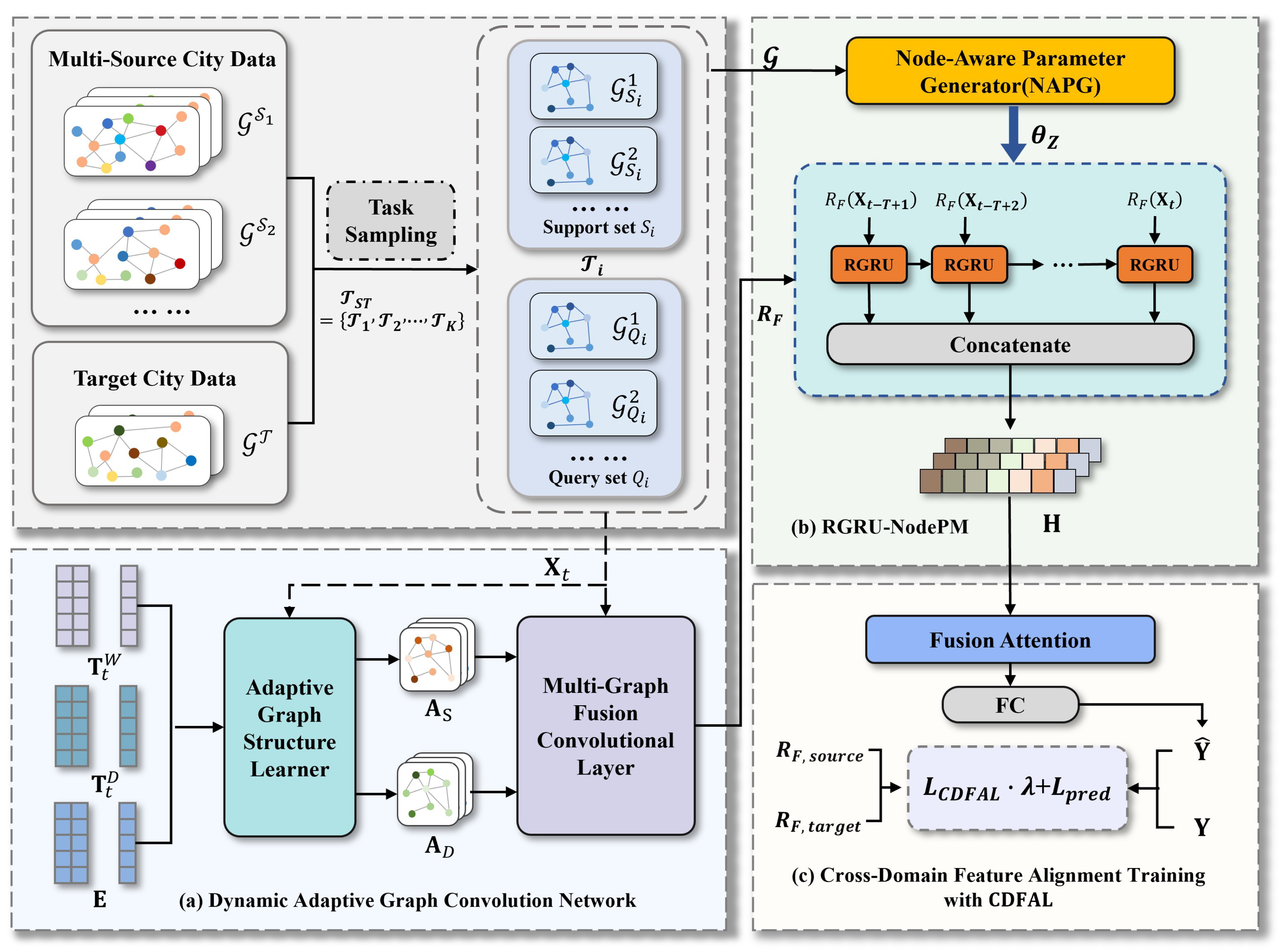
In this section, a detailed description of our proposed method, DGCTF, is presented. As shown in Figure 2, DGCTF consists of a dynamic spatio-temporal graph convolution network, a RGRU-NodePM module, and is trained through a cross-domain feature alignment training method with CDFAL. The learning process of DGCTF follows MAML [37]. During the pre-training stage, the current flow ${\mathbf{X}}_t$ is used as input to the dynamic adaptive graph convolution network, as shown in Figure 2a. This network includes a adaptive graph structure learner and a multi-graph convolutional fusion layer. The initial node embedding $\mathbf{E}$ as well as the daily embedding ${\mathbf{T}}_t^D$ and the weekly embedding ${\mathbf{T}}_t^W$ are fed into the adaptive graph structure learner to generate both the dynamic adjacency matrix ${\mathbf{A}}_D$ and the static adjacency matrix ${\mathbf{A}}_S$, capturing both time-varying and stable spatial dependencies. The multi-graph convolutional fusion layer fuses the graph convolution results of ${\mathbf{A}}_S$ and ${\mathbf{A}}_D$ to generate the fused results $R_F$, which are then fed into the RGRU-NodePM module for further extraction of spatio-temporal dependencies. As shown in Figure 2b, RGRU-NodePM is designed to transfer knowledge across nodes through a node-level parameter matching strategy. Specifically, NAPG maps raw traffic inputs $\mathcal{G}$ to node-specific parameters ${\theta }_Z$ for the RGRU, which guaranties that nodes exhibiting analogous characteristics obtain comparable model parameters. In addition, as shown in Figure 2c, we design cross-domain feature alignment loss ${\mathcal{L}}_{CDFAL}$ based on covariance regularization for cross-domain feature alignment training to reduce global distribution differences among different cities at the domain level and ensure the transferability of the graph structure learner. Meanwhile, updated results $\mathbf{H}$ from the RGRU-NodePM are passed through the fusion attention module with both global and local attention to produce prediction loss ${\mathcal{L}}_{pred}$. The model is trained by the combination of ${\mathcal{L}}_{pred}$ and ${\mathcal{L}}_{CDFAL}$. In the fine-tuning phase, the model is trained with the target dataset ${\mathcal{G}}^{\mathcal{T}}$ to achieve parameter update with ${\mathcal{L}}_{pred}$.

Figure 2. The overall framework of DGCTF. (a) The architecture of the dynamic adaptive graph convolution network in DGCTF. (b) The architecture and the node-level parameter matching strategy of RGRU-NodePM. (c) The detail of the cross-domain feature alignment training with CDFAL.

4.1. Dynamic Adaptive Graph Convolution Network

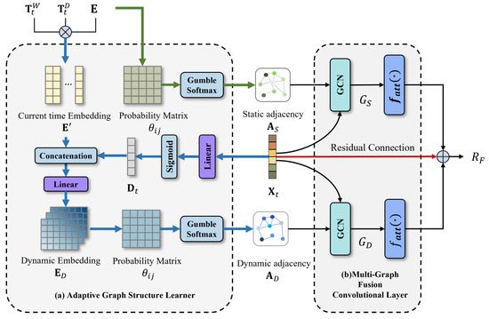
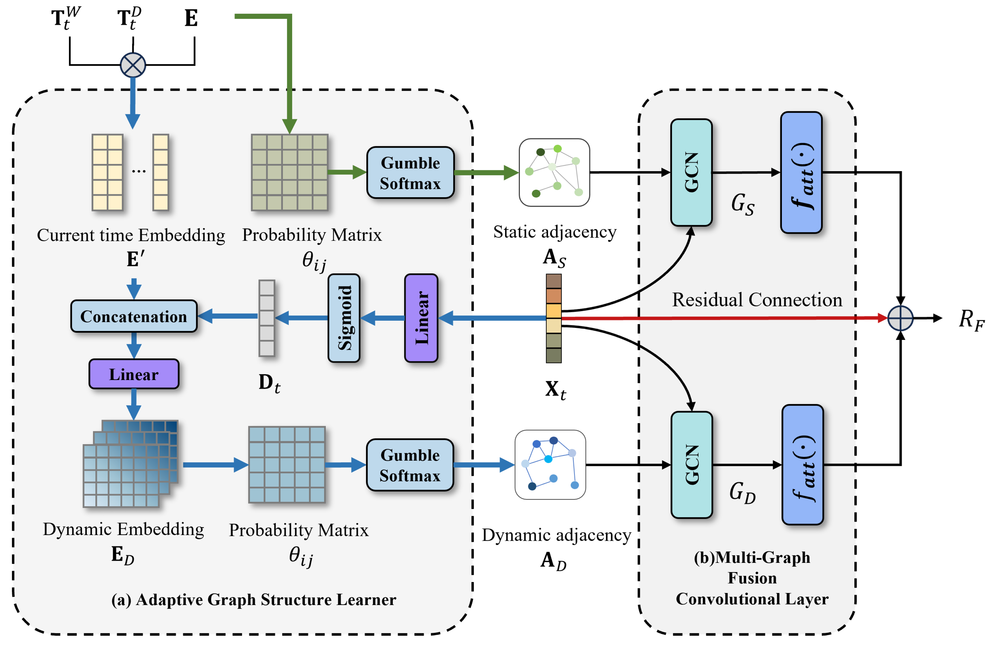
Most existing works [12,13,38] require a significantly large amount of parameters to learn evolving graph structures, which are prone to overfitting in cross-domain scenarios where the target city usually only has limited data [10]. To prevent overfitting and enhance feature retention, an adaptive graph structure learner and a multi-graph fusion convolutional layer with residual connection are designed to improve the model’s transferability and stability, as depicted in Figure 3. We will detail the two parts in the following sections.

Figure 3. Architecture of the (a) Adaptive Graph Structure Learner and (b) Multi-Graph Fusion Convolutional Layer. The green arrows indicate the construction process of the static adjacency matrix, where the initial node embedding $\mathbf{E}$ is used to construct ${\mathbf{A}}_S$. The blue arrows indicate the construction process of the dynamic adjacency matrix, where the initialize node embedding $\mathbf{E}$, daily embedding ${\mathbf{T}}_t^D$ and weekly embedding ${\mathbf{T}}_t^W$ are combined into the current time embedding ${\mathbf{E}}^{\prime }$. The current flow ${\mathbf{X}}_t$ is processed by a linear, then concatenated with ${\mathbf{E}}^{\prime }$ to generate the dynamic embedding ${\mathbf{E}}_D$ which is applied to construct ${\mathbf{A}}_D$.

4.1.1. Adaptive Graph Structure Learner

In order to enable the model to extract periodic and dynamic features of traffic signals and prevent overfitting in cross-domain scenarios, the adaptive graph structure learner leverages simple linear layers to directly capture inherent characteristics from time series $\mathbf{X}$ and guide the construction of a dynamic adjacency matrix.

Frist, to fully capture the periodic nature of traffic information, we fuse the initial node embedding $\mathbf{E}$ with daily embeddings ${\mathbf{T}}_t^D\in {\mathbb{R}}^{T\times N\times d_e}$ and weekly embeddings ${\mathbf{T}}_t^W\in {\mathbb{R}}^{T\times N\times d_e}$ by Hadamard product operation ⊙ to obtain the current time embedding ${\mathbf{E}}^{\prime }\in {\mathbb{R}}^{T\times N\times d_e}$:

$${\mathbf{E}}^{\prime }=\mathbf{E}\odot {\mathbf{T}}_t^D\odot {\mathbf{T}}_t^W.$$

(5)

At time step t, the current flow ${\mathbf{X}}_t\in {\mathbb{R}}^{N\times C}$ is processed through a linear transformation with sigmoid activation to obtain the dynamic signal ${\mathbf{D}}_t\in {\mathbb{R}}^{N\times d_e}$, which is then concatenated with the current time embedding ${\mathbf{E}}_t^{\prime }\in {\mathbb{R}}^{N\times d_e}$ to generate the dynamic embedding ${\mathbf{E}}_D\in {\mathbb{R}}^{N\times d_e}$:

$${\mathbf{D}}_t=\sigma \left(Linear\left({\mathbf{X}}_t\right)\right),$$

(6)

$${\mathbf{E}}_D=tanh\left(Linear(\mathbf{D}t\parallel {\mathbf{E}}_t^{\prime })\right),$$

(7)

where ‖ denotes the feature-wise concatenation along the embedding dimension.

As indicated by the flow of the blue arrows in Figure 3, then we use ${\mathbf{E}}_D$ which contains temporal information as input to derive the spatial probability matrix $\theta \in {\mathbb{R}}^{N\times N}$:

$$\theta ={\mathbf{E}}_D{\mathbf{E}}_D^T,$$

(8)

where ${\theta }_{ij}\in \theta$ represents the probability of preserving the edge between node i and node j.

Then, we apply Gumbel reparameterization trick [39] to learn the binary dynamic adjacency matrix ${\mathbf{A}}_D$ through ${\theta }_{ij}$, which is defined as:

$$\begin{array}{c}\hfill \begin{array}{c}\hfill {\mathbf{A}}_D=\sigma \left(\left(log\left({\theta }_{ij}/\left(1-{\theta }_{ij}\right)\right)+(g_{ij}^1-g_{ij}^2)\right)/s\right)\\ \hfill s.t.g_{ij}^1,g_{ij}^2\sim Gumbel(0,1),\end{array}\end{array}$$

(9)

where ${\mathbf{A}}_D\in {\mathbb{R}}^{N\times N}$, $\sigma$ denotes the sigmoid activation function, and s is the temperature parameter. Following the implementation in [39], s is set to 0.5, and hard sampling is used in the forward pass to obtain a binary ${\mathbf{A}}_D$, while the straight-through estimator is integrated to maintain backward differentiability via continuous gradients.

As indicated by the flow of the green arrows in Figure 3, then we use $\mathbf{E}$ as input to construct the static adjacency matrix ${\mathbf{A}}_S\in {\mathbb{R}}^{N\times N}$ in the same way as ${\mathbf{A}}_D$, which allows the model to capture stable spatial dependencies.

4.1.2. Multi-Graph Fusion Convolutional Layer

To prevent the smoothing effect in spatial feature extraction from impairing the model’s ability to predict peak values, we design a residual connection in the multi-graph fusion convolutional layer, as depicted in Figure 3b.

Firstly, we employ the first-order approximation of Chebyshev graph convolution to extract spatial features. The graph convolution operations are conducted on the static adjacency matrix ${\mathbf{A}}_S$ and ${\mathbf{A}}_D$ as follows:

$$G_S\left({\mathbf{X}}_t\right)=\left(\mathbf{I}+{\mathbf{D}}^{-{\displaystyle \frac{1}{2}}}{\mathbf{A}}_S{\mathbf{D}}^{-{\displaystyle \frac{1}{2}}}\right){\mathbf{X}}_t{\mathbf{W}}_S+{\mathbf{b}}_S,$$

(10)

$$G_D\left({\mathbf{X}}_t\right)=\left(\mathbf{I}+{\mathbf{D}}^{-{\displaystyle \frac{1}{2}}}{\mathbf{A}}_D{\mathbf{D}}^{-{\displaystyle \frac{1}{2}}}\right){\mathbf{X}}_t{\mathbf{E}}_S{\mathbf{W}}_D+{\mathbf{E}}_S{\mathbf{b}}_D,$$

(11)

where $G_S\left({\mathbf{X}}_t\right)\in {\mathbb{R}}^{B\times N\times F}$, $G_D\left({\mathbf{X}}_t\right)\in {\mathbb{R}}^{B\times N\times F}$, and ${\mathbf{W}}_S\in {\mathbb{R}}^{C\times F}$ and ${\mathbf{W}}_D\in {\mathbb{R}}^{d_e\times C\times F}$ are learnable weight matrices, ${\mathbf{b}}_S\in {\mathbb{R}}^F$ and ${\mathbf{b}}_D\in {\mathbb{R}}^{d_e\times F}$ are learnable bias matrices, F is the hidden layer dimension. $\mathbf{D}$ is the degree matrix. $\mathbf{I}$ is the unit matrix.

To further enhance the model’s ability to extract key features, we introduce a feature-recalibration operator $f_{att}(·)$ to refine the convolutional outputs. This module adaptively recalibrates feature responses by modeling inter-dependencies between channels. The operation of $f_{att}(·)$ is defined as:

$$f_{att}\left(\mathbf{H}\right)=\mathbf{H}\odot \sigma \left({\mathbf{W}}_2·\mathrm{ReLU}({\mathbf{W}}_1·\mathrm{Pool}\left(\mathbf{H}\right))\right)$$

(12)

where $\mathbf{H}\in {\mathbb{R}}^{B\times N\times F}$ represents the input hidden features, ${\mathbf{W}}_1\in {\mathbb{R}}^{F\times (F/r)}$ and ${\mathbf{W}}_2\in {\mathbb{R}}^{(F/r)\times 1}$. Here, r is the reduction ratio used to compress and then project the feature dimensions, which is set to 4 in our implementation, $\sigma (·)$ represent the Hardsigmoid function.

Then, we design a residual connection between the raw input and the graph convolution results to ensure the integration of low-level detail information with high-level semantic information, as shown in Figure 3b. The calculation could be formulated as:

$$R_F\left({\mathbf{X}}_t\right)=f_{\mathrm{att}}\left(G_S\left({\mathbf{X}}_t\right)\right)+f_{\mathrm{att}}\left(G_D\left({\mathbf{X}}_t\right)\right)+{\alpha }_F{\mathbf{X}}_t{\mathbf{W}}_F,$$

(13)

where $R_F\left({\mathbf{X}}_t\right)\in {\mathbb{R}}^{B\times N\times F}$ denotes the result of the fusion, ${\alpha }_F$ is a hyperparameter, ${\mathbf{W}}_F\in {\mathbb{R}}^{C\times F}$ is a training parameter matrix.

4.2. Residual-Enhanced GRU with Node-Level Parameter Matching Strategy

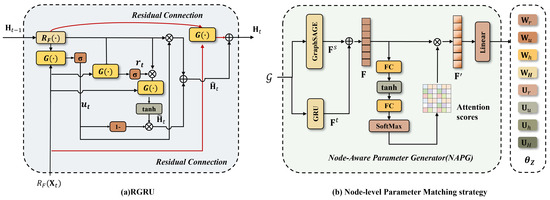
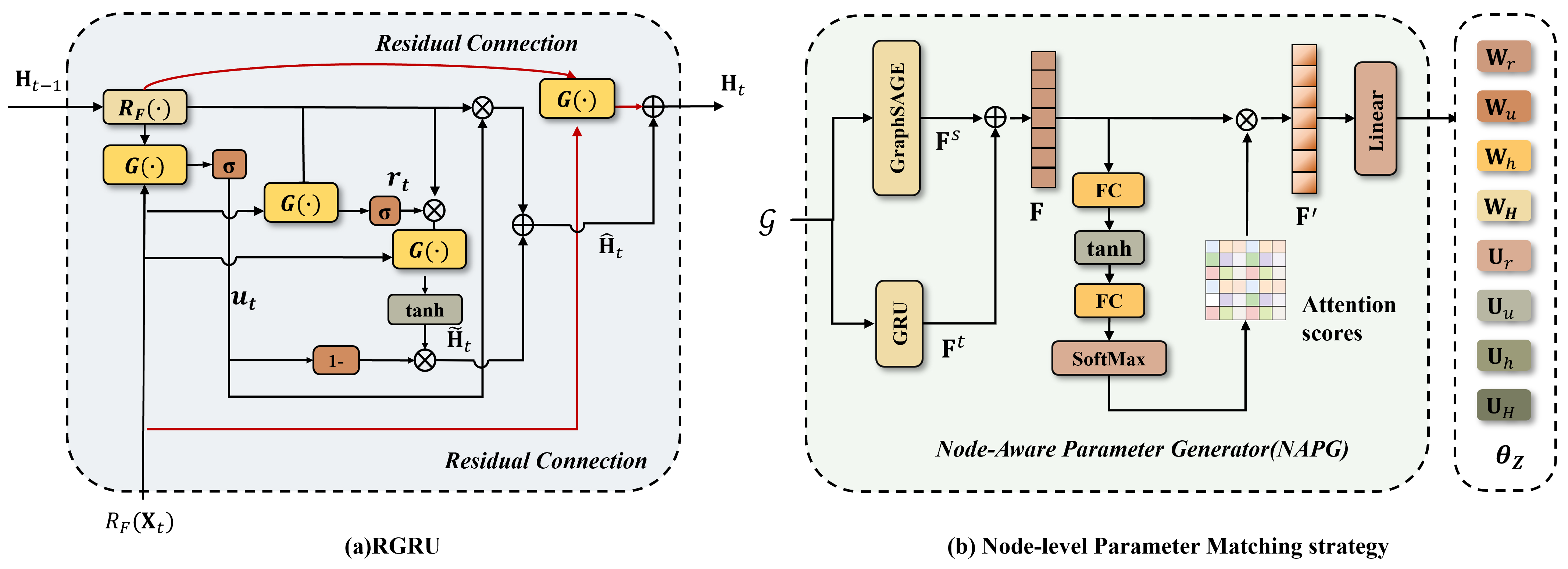
Previous transfer learning approaches [4,9,10] globally share the parameters of the feature extractors, which overlook the underlying correlations among nodes across source and target domains. To enable fine-grained knowledge transfer between similar nodes, an RGRU-NodePM is designed, as depicted in Figure 4, which integrates a residual-enhanced GRU with a node-level parameter matching strategy powered by a unified generator named NAPG.

Figure 4. Architecture of RGRU-NodePM. (a) RGRU with NP-LCU. (b) Details of the Node-level Parameter Matching strategy via NAPG. The weight matrices ${\theta }_Z=\{{\mathbf{W}}_r,{\mathbf{W}}_u,{\mathbf{W}}_h,{\mathbf{W}}_H,{\mathbf{U}}_r,{\mathbf{U}}_u,{\mathbf{U}}_h,{\mathbf{U}}_H\}$ in RGRU are node-specific and generated through the NAPG.

4.2.1. Architecture of RGRU

Unlike traditional GRU, where the weight matrices ${{\mathbf{W}}_0\in \mathbb{R}}^{B\times d_{\mathrm{in}}\times d_{\mathrm{out}}}$ and ${{\mathbf{U}}_0\in \mathbb{R}}^{B\times d_{\mathrm{in}}\times d_{\mathrm{out}}}$ in the linear layer are shared across all nodes and randomly initialized, we introduce a Node-level Parameter-matching Linear Combination Unit (NP-LCU) to replace the standard linear layer, as shown in Figure 4a.

The NP-LCU employs node-specific weight matrices ${\mathbf{W}\in \mathbb{R}}^{B\times N\times d_{\mathrm{in}}\times d_{\mathrm{out}}}$ and ${\mathbf{U}\in \mathbb{R}}^{B\times N\times d_{\mathrm{in}}\times d_{\mathrm{out}}}$, which are generated through NAPG, detailed later in Section 4.2.2. NP-LCU performs as:

$$G\left(x_1;x_2;\mathbf{W};\mathbf{U}\right)=\mathbf{W}·x_1+\mathbf{U}·x_2,$$

(14)

where ${x_1\in \mathbb{R}}^{B\times N\times d_{\mathrm{in}}}$, ${x_2\in \mathbb{R}}^{B\times N\times d_{\mathrm{in}}}$, ${G\in \mathbb{R}}^{B\times N\times d_{\mathrm{out}}}$.

To alleviate the decay effect of long-term modeling and enhance the feature-extraction ability, we design a residual connection to construct a residual GRU (RGRU), whose structure is shown in Figure 4a. The fusion convolutional results $R_F\left({\mathbf{X}}_t\right)$ and $R_{\mathrm{F}}\left({\mathbf{H}}_{t-1}\right)$ are passed through an NP-LCU and subsequently fused with the updated hidden state ${\widehat{\mathbf{H}}}_t$.

The RGRU takes the fusion result as input to dynamically update and integrate the information and extract both spatial and temporal dependencies. The update formula for RGRU is as follows:

$$r_t=\sigma \left(G\left(R_F\left({\mathbf{X}}_t\right);R_F\left({\mathbf{H}}_{t-1}\right);{\mathbf{W}}_r;{\mathbf{U}}_r\right)\right),$$

(15)

$$u_t=\sigma \left(G\left(R_F\left({\mathbf{X}}_t\right);R_F\left({\mathbf{H}}_{t-1}\right);{\mathbf{W}}_u;{\mathbf{U}}_u\right)\right),$$

(16)

$${\tilde{\mathbf{H}}}_t=tanh\left(G\left(R_F\left({\mathbf{X}}_t\right);r_t\odot R_F\left({\mathbf{H}}_{t-1}\right);{\mathbf{W}}_h;{\mathbf{U}}_h\right)\right),$$

(17)

$${\widehat{\mathbf{H}}}_t=u_t\odot R_F\left({\mathbf{H}}_{t-1}\right)+\left(1-u_t\right)\odot {\tilde{\mathbf{H}}}_t,$$

(18)

$${\mathbf{H}}_t={\widehat{\mathbf{H}}}_t+G\left({\alpha }_x{R}_F\left({\mathbf{X}}_t\right);{\alpha }_h{R}_F\left({\mathbf{H}}_{t-1}\right);{\mathbf{W}}_H;{\mathbf{U}}_H\right),$$

(19)

where ${\mathbf{X}}_t$ and ${\mathbf{H}}_t$ are input and output at step t, $\sigma$ denotes the sigmoid activation. ${\alpha }_h$ and ${\alpha }_x$ are the hyperparameters.

4.2.2. Node-Level Parameter Matching Strategy via NAPG

The node-level parameter matching strategy is designed to transfer knowledge at the node-level by enabling nodes with similar spatio-temporal features to receive similar model parameters. Here, “transferable knowledge” refers not to an explicit, human-readable knowledge bank, but to an abstract, data-driven parameterization transferable across domains. To achieve this, we design NAPG, as shown in Figure 4b, which maps raw traffic inputs $\mathcal{G}$ to node-specific parameters ${\theta }_Z{\in \mathbb{R}}^{B\times N\times d_{\mathrm{in}}\times d_{\mathrm{out}}}$ in two steps.

Firstly, we obtain the functional node representation for each node, denoted as $\mathbf{F}$. We employ GRU to capture temporal dynamics, and GraphSAGE to extract spatial dependencies. The two representations are fused through a weighted combination to form $\mathbf{F}$:

$${\mathbf{F}}^t=FC\left(GRU\left(\mathbf{X}\right)\right),$$

(20)

$${\mathbf{F}}^s=FC\left(GraphSAGE\left(\mathbf{X};\mathcal{E}\right)\right),$$

(21)

$$\mathbf{F}=a_z{\mathbf{F}}^t+\left(1-a_z\right)·{\mathbf{F}}^s,$$

(22)

where ${\mathbf{F}}^t\in {\mathbb{R}}^{B\times N\times d_m}$, ${\mathbf{F}}^s\in {\mathbb{R}}^{B\times N\times d_m}$, $\mathbf{F}\in {\mathbb{R}}^{B\times N\times d_m}$, $d_m$ represents the dimension of functional node representation, $a_z$ is a learnable ratio.

Then, we design an attention mechanism to emphasize task-relevant feature dimensions of functional node representation. We generate attention scores and apply them to $\mathbf{F}$ by the following formula:

$${\alpha }_i={\displaystyle \frac{exp\left({FC\left(tanh\right(FC(\mathbf{F}}_i\right)\left)\right))}{{\sum }_{j=1}^{d_m}exp({FC(tanh(FC(\mathbf{F}}_j)\left)\right))}},$$

(23)

$${\mathbf{F}}^{\prime }=\sum _{i=1}^{d_m}{\alpha }_i{\mathbf{F}}_i,$$

(24)

where ${\alpha }_i\in {\mathbb{R}}^{B\times N\times 1}$ is the attention score, ${\mathbf{F}}^{\prime }\in {\mathbb{R}}^{B\times N\times d_m}$ is the weighted representation of the functional node.

Subsequently, we generate parameters based on ${\mathbf{F}}^{\prime }$ through a linear transformation: ${\mathbb{R}}^{B\times N\times d_m}\to {\mathbb{R}}^{B\times N\times d_{\mathrm{in}}·d_{\mathrm{out}}}$, then reshape it to ${\mathbb{R}}^{B\times N\times d_{\mathrm{in}}\times d_{\mathrm{out}}}$.

$${\theta }_Z=\mathrm{Reshape}\left(Linear\left({\mathbf{F}}^{\prime }\right)\right).$$

(25)

Functional node representation $\mathbf{F}$ encompasses the unique spatio-temporal features of each node. By generating node-specific parameters from ${\mathbf{F}}^{\prime }$, the node-level parameter matching strategy directly bridges the spatio-temporal knowledge of the data with the model parameters, allowing nodes with similar spatio-temporal characteristics to share similar model parameters in a shared latent space, even without node semantic identities or equal graph sizes. This facilitates knowledge transfer between similar nodes across different cities.

4.3. Cross-Domain Feature Alignment Training

4.3.1. CDFAL Calculation

In transfer learning, the distribution differences between the source and target domains are a major challenge. Traditional adaptive transfer learning methods [4,10,36] aim to address these differences by constructing a shared feature space with metric loss or adversarial loss. However, in multi-source scenarios, adversarial-based methods require auxiliary domain discriminators, and the dynamic alternation of source domains across various meta-tasks often leads to training instability and mode collapse. Meanwhile, approaches based on MMD are heavily constrained by sensitive kernel selection and the complexities of parameter tuning. Consequently, these traditional approaches are frequently ineffective for robust knowledge transfer in multi-source settings. To overcome these limitations and facilitate effective domain-level knowledge transfer in multi-source city settings, we propose the CDFAL:

$${\mathcal{L}}_{CDFAL}={\displaystyle \frac{1}{4F^2}}{∥C\left(R_{F,source}\right)-C\left(R_{F,target}\right)∥}_F^2,$$

(26)

where ${\Vert ·\Vert }_F^2$ denotes the squared matrix Frobenius norm. $C(·)$ represents the covariance matrix calculation, as adopted from [40]. CDFAL explicitly optimizes the second-order statistics of feature distributions through parameter-free covariance alignment, offering high computational efficiency and stability. It is particularly well-suited for multi-batch sampling in meta-training, eliminating the complexity of kernel selection.

During each task ${\mathcal{T}}_i$ of the pre-training stage, a source city is randomly selected. We measure the covariance distance between the fused graph convolution results $R_{F,source}$ of the selected source city and $R_{F,target}$ of the target city through CDFAL. This process of random sampling and feature alignment reduces the feature distance between the source and target cities in a systematic, incremental fashion, and ensures the transferability of the graph structure learner. Crucially, this transferability resides in the learner’s universal mapping logic for capturing spatio-temporal correlations rather than the specific numerical values of the generated adjacency matrix. Specifically, the gradients from CDFAL propagate back to the adaptive graph structure learner through the backpropagation path, effectively regularizing its structural mapping logic to prioritize adjacency matrices that yield domain-invariant feature representations across heterogeneous urban layouts. As the model progresses through the pre-training stage, it gradually decreases the domain-level feature differences among all the pre-trained cities.

4.3.2. Fusion Attention Module

The traffic state at a certain moment is influenced by the traffic conditions of multiple preceding moments and is relatively more affected by recent time steps [27]. Motivated by this intuition, we design a task-specific fusion attention module consisting of global attention and local attention, which is placed after the RGRU-NodePM to handle hidden states, as shown in Figure 2c. Specifically, the hidden representations from the previous $T_g$ steps are used in global attention to capture long-term patterns, while the most recent $T_l$ steps are used in local attention to focus on short-term dynamics. Since the structure of the traffic network and traffic condition contribute to predicting future states [41], we incorporate the intrinsic network information and traffic condition information by concatenating the initial node embedding $\mathbf{E}$ with hidden states $\mathbf{H}$ to obtain the attention score. The attention scores of the global attention and the local attention are obtained through the following formula:

$$o_{i,j}={\displaystyle \frac{⟨{\mathbf{W}}_q\left[{\mathbf{H}}_i^o·{\mathbf{E}}_i\right],{\mathbf{W}}_k\left[{\mathbf{H}}_j^o·{\mathbf{E}}_j\right]⟩}{\sqrt{d}}},$$

(27)

$${\gamma }_{i,j}={\displaystyle \frac{exp\left(o_{i,j}\right)}{{\sum }_{k\le N}exp\left(o_{i,j}\right)}},$$

(28)

where $⟨,⟩$ denotes the inner product, ${\mathbf{E}}_i$ is the node embedding of node i,${\mathbf{H}}_i^o$ represents the concatenated hidden states of node i over $T_g=12$ steps (for local attention, $T_l=3$ steps). ${\mathbf{W}}_q$ and ${\mathbf{W}}_k$ are the linear projection parameters, and d is the dimension of the query and key.

The attention scores are used as weights to compute the weighted sum of the hidden states of each node in the network:

$${\mathbf{H}}_i^{\prime }=\sum _{j\le N}{\gamma }_{i,j}·{\mathbf{H}}_j^o.$$

(29)

Then, we obtain the weighted sums ${\mathbf{H}}_{\mathrm{global}}^{\prime }\in {\mathbb{R}}^{N\times T_g\times C}$, ${\mathbf{H}}_{\mathrm{local}}^{\prime }\in {\mathbb{R}}^{N\times T_l\times C}$ of the global hidden states and the local hidden states for the nodes. By applying a linear transformation, we respectively convert them to ${\mathbf{H}}_{\mathrm{global}}^{″}\in {\mathbb{R}}^{N\times P\times C}$, ${\mathbf{H}}_{\mathrm{local}}^{″}\in {\mathbb{R}}^{N\times P\times C}$, to obtain the traffic predictions for P time steps for all nodes. Finally, we fuse the attention results to get the final prediction:

$$\widehat{\mathbf{Y}}={\lambda }_f{\mathbf{H}}_{\mathrm{global}}^{″}+\left(1-{\lambda }_f\right){\mathbf{H}}_{\mathrm{local}}^{″},$$

(30)

where ${\lambda }_f\in \left(0,1\right)$ is a hyperparameter, $\widehat{\mathbf{Y}}=\left[{\widehat{\mathbf{X}}}_{t+1},{\widehat{\mathbf{X}}}_{t+2},\cdots ,{\widehat{\mathbf{X}}}_{t+P}\right]\in {\mathbb{R}}^{N\times P\times C}$ is the forecasting result. Given the ground truth $\mathbf{Y}=\left[{\mathbf{X}}_{t+1},{\mathbf{X}}_{t+2},\cdots ,{\mathbf{X}}_{t+P}\right]\in {\mathbb{R}}^{N\times P\times C}$, the mean squared error (MSE) is utilized as the prediction loss ${\mathcal{L}}_{pred}$, which is defined as:

$${\mathcal{L}}_{pred}={\displaystyle \frac{1}{NPC}}\sum _{i=1}^N\sum _{j=1}^P\sum _{k=1}^C{({\widehat{\mathbf{Y}}}_{i,j,k}-{\mathbf{Y}}_{i,j,k})}^2.$$

(31)

4.4. DGCTF Learning Process

Recent studies have explored the integration of meta-learning with unsupervised domain adaptation (UDA) to mitigate distribution shifts and migration noise by incorporating unlabeled target domain information during the pre-training process [42]. Inspired by this, we adopt an unsupervised meta-adaptation strategy for DGCTF. The learning process can be divided into pre-training and fine-tuning stages. The pre-training stage is summarized in Algorithm 1.

The objective of the pre-training stage is to learn a well-generalized initialization $\theta$. To achieve this, we construct a meta-task pool ${\mathcal{T}}_{ST}=\{{\mathcal{T}}_1,{\mathcal{T}}_2,\dots ,{\mathcal{T}}_K\}$ based on the following task sampling and partitioning protocol.

In each training iteration, a meta-task ${\mathcal{T}}_i$ is formed by randomly sampling a source city ${\mathcal{G}}^{{\mathcal{S}}_j}$ from the source city pool ${\mathcal{G}}^{\mathcal{S}}$ and pairing it with the target city ${\mathcal{G}}_u^{\mathcal{T}}$. Crucially, ${\mathcal{G}}_u^{\mathcal{T}}$ is strictly composed of unlabeled graph sequences sampled from the target city’s few-shot training pool. Each task consists of 2m graph sequences drawn from both the sampled source city and the target city training pool. The sequences from the source and target domains are symmetrically partitioned into a support set ${\mathcal{S}}_i$ and a query set ${\mathcal{Q}}_i$. Specifically, in the source domain, both the support set ${\mathcal{G}}_{S_i}^{{\mathcal{S}}_j}$ and the query set ${\mathcal{G}}_{Q_i}^{{\mathcal{S}}_j}$ are fully labeled to provide supervised guidance. Conversely, in the target domain, the labels for the support set ${\mathcal{G}}_{S_i}^{\mathcal{T}}$ and the query set ${\mathcal{G}}_{Q_i}^{\mathcal{T}}$ are strictly hidden. This setup ensures that the model is meta-trained to adapt in an “unsupervised” manner. For each task ${\mathcal{T}}_i$, the model first performs inner-loop updates using the support set $S_i$, and then evaluates the adapted parameters on the corresponding query set $Q_i$ for outer-loop meta-optimization. During this stage, the model considers a combined loss that incorporates both prediction error loss ${\mathcal{L}}_{pred}$ and the proposed cross-domain feature alignment loss ${\mathcal{L}}_{CDFAL}$. Consequently, the joint loss funtion $\mathcal{L}$ is:

$$\mathcal{L}={\mathcal{L}}_{pred}+\lambda {\mathcal{L}}_{CDFAL},$$

(32)

where $\lambda$ is a hyperparameter.

In the fine-tuning stage, the model undergoes multiple gradient descents on the target dataset to achieve parameter updating. In this stage, the optimization objective focuses solely on the prediction error:

$$\mathcal{L}={\mathcal{L}}_{pred}.$$

(33)

Algorithm 1 DGCTF Pre-training Stage

Require:  Source cities ${\mathcal{G}}^{\mathcal{S}}=\{{\mathcal{G}}^{{\mathcal{S}}_1},\dots ,{\mathcal{G}}^{{\mathcal{S}}_M}\}$; Unlabeled target city sequences ${\mathcal{G}}_u^{\mathcal{T}}$; Learning rates $\alpha ,\beta$; Alignment weight $\lambda$. Ensure:  Well-generalized initialization parameters $\theta$.  1: Randomly initialize $\theta$;  2: while not done do  3:    Sample a source city ${\mathcal{G}}^{{\mathcal{S}}_j}\sim {\mathcal{G}}^{\mathcal{S}}$ and pair it with ${\mathcal{G}}_u^{\mathcal{T}}$ to form meta-tasks ${\mathcal{T}}_{ST}$;  4:    for each task ${\mathcal{T}}_i\in {\mathcal{T}}_{ST}$ do  5:      Form $S_i=\{{\mathcal{G}}_{S_i}^{\mathcal{S}},{\mathcal{G}}_{S_i}^{\mathcal{T}}\}$ and $Q_i=\{{\mathcal{G}}_{Q_i}^{\mathcal{S}},{\mathcal{G}}_{Q_i}^{\mathcal{T}}\}$;  6:      Compute inner loss: $\mathcal{L}(\theta ,S_i)={\mathcal{L}}_{pred}(\theta ,{\mathcal{G}}_{S_i}^{\mathcal{S}})+\lambda {\mathcal{L}}_{CDFAL}(\theta ,{\mathcal{G}}_{S_i}^{\mathcal{S}},{\mathcal{G}}_{S_i}^{\mathcal{T}})$;  7:      Update ${\varphi }_i\leftarrow \theta -\alpha {\nabla }_{\theta }\mathcal{L}(\theta ,{\mathcal{S}}_i)$;  8:      Compute outer loss: $\mathcal{L}({\varphi }_i,Q_i)={\mathcal{L}}_{pred}({\varphi }_i,{\mathcal{G}}_{Q_i}^S)+\lambda {\mathcal{L}}_{CDFAL}({\varphi }_i,{\mathcal{G}}_{Q_i}^{\mathcal{S}},{\mathcal{G}}_{Q_i}^{\mathcal{T}})$;  9:     end for 10:    Update $\theta \leftarrow \theta -\beta {\nabla }_{\theta }{\sum }_i\mathcal{L}({\varphi }_i,Q_i)$; 11: end while 12: eturn $\theta$;

5. Experiments

In this section, we evaluate DGCTF in various aspects through extensive experiments. Specifically, we try to answer the following research questions through our evaluation:

• RQ1: How well does DGCTF perform against other baselines on different datasets under conditions of target domain data scarcity?
• RQ2: How well does each proposed component of the model contribute to the performance of DGCTF?
• RQ3: How does the amount of training data affect the performance of DGCTF?
• RQ4: How does each major hyperparameter affect the performance of DGCTF?
• RQ5: How robust is DGCTF when the source–target distribution gap becomes larger?

5.1. Datasets

We evaluate the performance of DGCTF on seven popular public real-world datasets of two categories: (1) traffic flow and (2) traffic speed. The traffic flow datasets are PEMS04, PEMS07, and PEMS08 [43]. The traffic speed datasets are METR-LA, PEMS-BAY [20], Chengdu, Shenzhen [44]. Detailed information of these datasets is shown in Table 1.

Table 1. Statistics of the seven datasets used in this paper.

Dataset		Nodes	Edges	Days	Interval
Traffic Flow	PEMS04	307	340	59	5 min
	PEMS07	883	866	98	5 min
	PEMS08	170	295	62	5 min
Traffic Speed	METR-LA	207	1515	119	5 min
	PEMS-BAY	325	2369	180	5 min
	Chengdu	524	596	120	10 min
	Shenzhen	627	4218	120	10 min

In transfer learning, there are source datasets and a target dataset. We use a similar few-shot traffic forecasting setting to [8]. Taking PEMS04 as an example, when it is set as the target city, ten days of data from PEMS04 are selected as the target data for fine-tuning, and the remaining data of PEMS04 constitutes the test data. The other two datasets (PEMS07, PEMS08) are used as source datasets for training with the full data, as shown in Table 1. For traffic flow prediction tasks, we set PEMS04, PEMS07 and PEMS08 respectively as target city, with the other two serving as source datasets. For traffic speed prediction tasks, we set METR-LA and PEMS-BAY respectively as target city, with the other three serving as source datasets. Z-score normalization is applied for data preprocessing.

5.2. Experimental Settings

For traffic flow data, we use ten-day data from the target city for fine-tuning and utilize one-hour historical data to forecast for the next 15, 30, and 60 min (horizon = 3, 6, and 12, respectively). For traffic speed datasets, we use three-day data from the target city to fine-tune and predict traffic speed for the next 6 time steps using 12 historical time steps. All experiments are executed on a Linux server (CPU: Intel^® Xeon^® Gold 5317 CPU@3.0 GHz, GPU: NVIDIA A100). The task learning rate $\alpha$ = 0.01, the meta-training rate $\beta$ = 0.001, the number of task batches m is set to 4, and the number of pre-training tasks K is set to 200. The residual connection weights ${\alpha }_F$, ${\alpha }_h$, and ${\alpha }_x$ are all set to 0.1. The hidden layer dimension F is set to 16. The Adam optimizer of the fine-tuning has a learning rate of 0.001 and weight decay of 0.01. The early stopping is adopted with a patience setting of 20 to avoid overfitting. We evaluate the prediction performance using root mean squared error (RMSE), mean absolute error (MAE), and mean absolute percentage error (MAPE).

5.3. Baselines

To ensure a rigorous and unbiased evaluation, we select representative baseline models that are extensively utilized in the field of traffic forecasting. Our objective is to assess the effectiveness of DGCTF under an equivalent information budget, specifically within the context of limited target domain data. Following established paradigms in cross-city traffic forecasting research [4,36], we categorize the selected baselines into three major categories: traditional, non-transfer deep learning-based, and transfer deep learning-based methods.

(1) Traditional baselines:

• HA [45]: Historical Average method uses the average value of historical traffic data to predict future traffic flow.

(2) Non-transfer deep learning-based baselines:

• GRU [46]: Gated Recurrent Unit, a variant of RNN with strong capability to capture temporal dependencies.
• GCN [47]: Graph Convolutional Network, with strong capability to capture spatial dependencies.
• TGCN [19]: Temporal Graph Convolutional Network, known for its excellent short-term prediction capability.
• STGCN [18]: Spatial-Temporal Graph Convolutional Network, uses CHEBNET and 2D convolution for traffic prediction.
• DCRNN [20]: Diffusion Convolutional Recurrent Neural Network, combines GNN and RNN with diffusion convolution.
• AGCRN [23]: Adaptive Graph Convolutional Recurrent Network, learns node patterns through node adaptive parameter learning and adaptive graph learning.
• STGODE [25]: Spatial-Temporal Graph Ordinary Differential equation Network, captures spatial-temporal dynamics using tensor-based ODE.
• DDGCRN [30]: Decomposition Dynamic Graph Convolutional Recurrent Network, captures spatial-temporal dynamics through the combination of dynamic graph convolution and GRU.
• TimeMixer [48]: Decomposable multiscale mixing for time series forecasting, demonstrates powerful predictive capabilities in data-scarce scenarios through a fully MLP-based lightweight architecture.

(3) Transfer deep learning-based baselines (including fine-tuning and state-of-the-art transfer learning methods):

• Fine-tuning Methods: The model is first pre-trained on the source city with sufficient data, and then fine-tuned on the target city with limited data. We select TGCN, AGCRN, and DDGCRN as fine-tuning baselines, respectively denoted as TGCN-FT, AGCRN-FT, and DDGCRN-FT.
• MAML [37]: Model-Agnostic, an excellent meta-learning method that pre-trains a well-generalized initial model, which can quickly adapt to new tasks in the target domain.
• ST-GFSL [8]: Spatio-Temporal Graph Few-Shot Learning, enhances feature extraction by learning node-level knowledge, which is a cross-city knowledge transfer framework based on MAML.
• DASTNET [9]: Domain Adversarial Spatial-Temporal Network, learns domain-invariant node embeddings across multiple source and target domains through domain adversarial learning.
• TPB [14]: Traffic Pattern Bank, forms a traffic pattern bank by clustering the knowledge of source cities to guide the learning of the target city.
• MTPB [15]: Multi-scale Traffic Pattern Bank, an improvement on TPB, uses clustering techniques to generate a multi-scale traffic pattern bank.
• STGP [35]: Spatio-Temporal Graph Prompting, a prompt-based framework capable of adapting to multi diverse tasks in a data-scarce domain.
• MC-HSTA [49]: Multi-source Cross-domain Hybrid Spatio-Temporal Attention network, captures inter-domain dependencies via attention and mitigates domain shift with an adversarial domain-adaptive classifier.

5.4. Performance Comparison and Analysis

We implement DGCTF and compare it with different methods on traffic flow and traffic speed datasets. We repeat the experiments five times and report the average results along with their standard deviations. The performance results are illustrated in Table 2 and Table 3. According to the results, we have the following observations.

Table 2. Performance comparison of different methods for traffic flow prediction. (The best results are marked in bold and the second-best results are underlined).

Models		PEMS04
		15 min			30 min			60 min
		MAE	RMSE	MAPE (%)	MAE	RMSE	MAPE (%)	MAE	RMSE	MAPE (%)
Traditional	HA [45]	28.36	40.55	20.14	31.75	45.14	22.84	38.52	54.45	28.48
Non-Transfer	GRU [46]	20.96	31.08	14.78	22.71	33.77	16.54	26.25	38.87	18.66
	GCN [47]	48.65	68.89	40.53	49.49	69.97	41.42	51.63	72.65	44.03
	TGCN [19]	24.09	34.31	18.26	25.22	36.09	19.34	27.16	38.76	20.84
	STGCN [18]	27.03	38.26	25.16	27.91	39.65	25.33	35.55	49.12	37.74
	DCRNN [20]	23.73	34.27	18.84	26.68	37.63	21.39	33.79	46.70	29.68
	AGCRN [23]	24.58	42.30	14.93	26.53	48.05	15.30	30.06	52.19	16.67
	STGODE [25]	20.73	31.97	15.79	23.14	35.55	17.66	27.24	41.05	23.86
	DDGCRN [30]	20.22	34.68	12.44	21.14	36.28	13.86	23.34	38.96	14.87
	TimeMixer [48]	18.97	29.67	12.33	19.81	32.11	13.28	21.94	33.88	15.12
Transfer	TGCN-FT [19]	20.22	32.58	13.07	21.63	34.42	14.03	24.67	38.51	16.14
	AGCRN-FT [23]	19.40	31.04	12.76	20.88	33.29	13.68	22.70	36.03	14.69
	DDGCRN-FT [30]	18.99	30.44	12.58	19.70	32.58	13.07	21.87	34.72	13.91
	ST-GFSL [8]	20.32	31.78	13.92	22.07	34.30	14.70	26.36	39.63	19.07
	DASTNET [9]	19.25	28.98	13.30	20.67	30.78	14.56	22.82	33.77	16.10
	TPB [14]	19.80	31.26	13.84	21.34	33.76	14.44	24.59	36.70	17.99
	MTPB [15]	18.96	30.61	13.48	20.60	32.40	15.23	23.04	35.72	16.77
	STGP [35]	19.92	30.68	13.50	21.28	32.28	14.12	22.57	33.87	15.14
	MC-HSTA [49]	18.97	28.41	12.67	20.24	30.41	13.76	22.17	33.46	15.67
	MAML [37]	19.05	30.15	12.60	20.26	31.82	13.65	22.42	34.74	14.66
	DGCTF (proposed)	18.03	27.91	11.91	19.21	29.97	12.01	20.61	32.76	13.07
	Std.Dev.	0.09	0.11	0.14	0.07	0.13	0.16	0.08	0.14	0.22
Models		PEMS07
		15 min			30 min			60 min
		MAE	RMSE	MAPE (%)	MAE	RMSE	MAPE (%)	MAE	RMSE	MAPE (%)
Traditional	HA [45]	32.85	46.56	15.10	37.09	52.38	17.26	45.43	63.90	21.66
Non-Transfer	GRU [46]	23.77	34.49	11.21	25.31	37.84	12.87	29.39	43.89	13.12
	GCN [47]	50.81	71.67	36.47	51.94	73.18	39.10	55.09	77.15	41.46
	TGCN [19]	30.18	42.11	15.74	30.84	43.58	16.19	33.25	47.24	16.58
	STGCN [18]	34.14	48.58	19.67	39.50	49.37	20.03	43.45	60.67	27.57
	DCRNN [20]	26.66	37.66	16.68	31.06	43.38	19.94	51.06	66.26	48.29
	AGCRN [23]	35.15	64.08	11.88	35.10	63.78	11.98	39.00	68.44	13.98
	STGODE [25]	22.30	33.89	10.92	26.02	38.52	14.23	30.87	45.27	17.21
	DDGCRN [30]	22.97	41.12	8.88	25.48	43.83	9.77	28.09	48.49	11.00
	TimeMixer [48]	21.17	33.53	9.28	24.25	36.87	11.44	29.96	44.41	14.01
Transfer	TGCN-FT [19]	23.38	39.39	9.40	25.39	41.87	10.27	29.70	47.13	12.27
	AGCRN-FT [23]	21.89	35.62	9.12	24.13	39.14	10.19	27.72	44.90	11.53
	DDGCRN-FT [30]	20.46	33.14	8.57	22.98	38.28	9.58	25.24	41.49	10.93
	ST-GFSL [8]	21.74	33.40	9.39	24.48	37.45	10.96	29.87	44.46	13.37
	DASTNET [9]	20.91	31.85	8.95	22.96	34.90	9.87	26.88	40.12	11.75
	TPB [14]	20.54	32.08	9.02	22.33	35.09	11.02	25.75	39.72	12.83
	MTPB [15]	20.34	31.69	9.29	21.92	34.02	9.75	24.67	38.14	11.82
	STGP [35]	20.85	32.17	10.40	22.22	33.95	11.13	24.69	38.20	12.72
	MC-HSTA [49]	20.31	31.64	8.82	22.04	34.69	9.51	26.75	39.22	11.40
	MAML [37]	20.23	32.21	8.70	22.68	35.76	9.81	26.44	41.12	11.38
	DGCTF (proposed)	19.32	30.92	8.01	21.13	32.79	8.89	23.85	37.63	10.01
	Std.Dev.	0.04	0.14	0.13	0.10	0.13	0.19	0.07	0.22	0.50
Models		PEMS08
		15 min			30 min			60 min
		MAE	RMSE	MAPE (%)	MAE	RMSE	MAPE (%)	MAE	RMSE	MAPE (%)
Traditional	HA [45]	23.12	33.03	14.61	26.12	37.16	16.55	32.15	45.41	20.60
Non-Transfer	GRU [46]	16.69	24.72	11.05	18.89	28.14	13.45	20.94	31.32	15.20
	GCN [47]	64.63	87.30	90.30	65.09	87.87	91.64	66.24	89.21	94.01
	TGCN [19]	20.65	28.77	15.06	21.60	30.40	15.97	24.33	34.20	17.91
	STGCN [18]	25.59	35.58	18.91	26.20	36.52	17.73	31.89	43.94	20.99
	DCRNN [20]	20.61	29.30	20.36	23.23	32.76	24.53	39.14	51.97	47.92
	AGCRN [23]	18.50	30.76	10.77	19.45	32.34	11.30	23.44	37.55	13.71
	STGODE [25]	20.42	37.92	17.82	23.41	36.41	21.00	26.86	39.85	24.43
	DDGCRN [30]	16.14	26.26	9.94	18.35	30.09	10.91	20.80	34.13	12.45
	TimeMixer [48]	15.52	24.48	9.44	18.50	29.40	10.81	20.89	32.65	12.68
Transfer	TGCN-FT [19]	16.81	26.29	10.52	18.09	29.27	11.01	22.00	35.84	13.74
	AGCRN-FT [23]	15.88	24.49	10.17	17.57	27.18	10.77	20.34	31.81	12.12
	DDGCRN-FT [30]	14.62	22.85	9.10	16.97	26.66	10.44	18.91	30.34	11.50
	ST-GFSL [8]	16.08	24.59	9.91	18.14	28.08	11.03	21.72	33.29	13.31
	DASTNET [9]	15.26	22.70	9.64	16.41	24.57	10.46	18.84	28.06	11.72
	TPB [14]	14.94	23.55	10.45	16.99	26.58	10.88	19.41	30.75	12.44
	MTPB [15]	14.63	22.13	10.07	15.82	24.68	10.61	18.51	29.38	12.31
	STGP [35]	15.82	22.96	10.33	16.74	24.91	10.54	18.85	28.30	12.35
	MC-HSTA [49]	14.90	22.01	9.11	16.02	24.34	10.47	18.64	28.03	11.44
	MAML [37]	14.83	22.93	10.14	16.40	25.49	10.50	18.63	28.99	11.79
	DGCTF (proposed)	13.42	21.05	8.31	15.01	23.47	9.30	17.44	27.36	10.45
	Std.Dev.	0.11	0.17	0.21	0.15	0.23	0.25	0.12	0.17	0.28

Table 3. Performance comparison of different methods for traffic speed prediction. (The best results are marked in bold and the second-best results are underlined).

Models		METR-LA
		5 min			15 min			30 min
		MAE	RMSE	MAPE (%)	MAE	RMSE	MAPE (%)	MAE	RMSE	MAPE (%)
Traditional	HA [45]	3.97	7.37	8.34	4.27	8.05	9.61	4.66	8.76	12.55
Non-Transfer	GRU [46]	2.45	4.14	6.00	3.01	5.63	7.93	3.73	6.97	10.29
	GCN [47]	2.48	4.66	6.17	3.07	6.19	8.04	3.70	7.62	9.96
	TGCN [19]	2.55	4.27	6.00	3.11	5.87	7.82	3.76	7.46	9.74
	STGCN [18]	2.33	4.11	5.82	2.92	5.78	7.68	3.59	7.31	9.90
	DCRNN [20]	2.63	4.98	6.43	3.43	7.07	8.88	4.34	8.91	11.62
	AGCRN [23]	2.52	4.33	6.39	3.04	5.80	8.06	3.64	7.22	10.00
	STGODE [25]	2.51	4.08	5.98	3.14	5.61	8.01	3.83	6.88	10.45
	DDGCRN [30]	2.49	4.25	6.24	3.10	5.73	8.13	3.64	7.12	9.94
	TimeMixer [48]	2.38	4.23	5.82	2.99	5.69	7.67	3.64	7.11	9.78
Transfer	TGCN-FT [19]	2.51	4.31	6.64	3.06	5.82	8.35	3.68	7.29	10.26
	AGCRN-FT [23]	2.49	4.28	6.16	3.03	5.78	7.87	3.63	7.22	9.84
	DDGCRN-FT [30]	2.45	4.23	6.22	3.01	5.66	7.91	3.61	7.07	9.88
	ST-GFSL [8]	2.43	4.23	6.30	3.03	5.72	8.11	3.87	7.28	10.39
	DASTNET [9]	2.44	4.33	6.57	3.03	5.88	8.48	3.63	7.29	10.43
	TPB [14]	2.39	4.13	6.28	2.90	5.55	8.09	3.69	6.91	10.35
	MTPB [15]	2.31	4.10	5.62	2.83	5.51	7.09	3.54	6.89	9.96
	STGP [35]	2.34	4.12	6.21	2.87	5.57	7.70	3.52	6.96	10.04
	MC-HSTA [49]	2.36	4.20	5.57	2.84	5.62	7.28	3.44	6.90	9.48
	MAML [37]	2.29	4.11	5.82	2.81	5.53	7.13	3.50	6.92	8.99
	DGCTF (proposed)	2.12	3.87	5.39	2.47	5.33	6.89	3.14	6.76	8.55
	Std.Dev.	0.01	0.03	0.01	0.02	0.04	0.03	0.02	0.03	0.02
Models		PEMS-BAY
		5 min			15 min			30 min
		MAE	RMSE	MAPE (%)	MAE	RMSE	MAPE (%)	MAE	RMSE	MAPE (%)
Traditional	HA [45]	2.67	5.49	5.19	2.95	6.01	6.34	3.23	6.56	7.01
Non-Transfer	GRU [46]	1.11	2.04	2.65	1.62	3.31	3.75	2.13	4.70	4.95
	GCN [47]	1.62	4.73	4.67	2.07	4.73	4.67	2.45	5.65	5.55
	TGCN [19]	1.21	2.11	2.38	1.68	3.48	3.48	2.19	4.91	4.76
	STGCN [18]	1.20	1.95	2.29	1.73	3.45	3.44	2.33	5.00	4.86
	DCRNN [20]	1.67	3.32	3.92	2.03	4.18	4.48	2.43	5.12	5.91
	AGCRN [23]	1.25	2.34	2.79	1.64	3.58	3.82	2.17	4.88	5.02
	STGODE [25]	1.06	1.80	2.14	1.61	3.22	3.55	2.17	4.59	5.07
	DDGCRN [30]	1.14	2.05	2.59	1.62	3.34	3.64	2.12	4.68	4.91
	TimeMixer [48]	1.09	2.09	2.19	1.63	3.45	3.51	2.19	4.79	5.09
Transfer	TGCN-FT [19]	1.18	2.16	2.57	1.67	3.45	3.67	2.18	4.83	4.92
	AGCRN-FT [23]	1.16	2.09	2.53	1.62	3.39	3.60	2.11	4.73	4.83
	DDGCRN-FT [30]	1.13	2.03	2.54	1.59	3.32	3.62	2.08	4.66	4.85
	ST-GFSL [8]	1.18	2.01	2.34	1.73	3.19	3.41	2.22	4.57	4.63
	DASTNET [9]	1.04	2.04	2.10	1.62	3.55	3.46	2.17	4.97	4.85
	TPB [14]	1.07	1.88	2.30	1.57	3.13	3.30	2.06	4.27	4.50
	MTPB [15]	1.02	1.76	1.97	1.51	3.10	3.28	2.02	4.24	4.47
	STGP [35]	1.12	1.85	2.09	1.59	3.09	3.33	2.12	4.28	4.79
	MC-HSTA [49]	0.96	1.72	1.92	1.47	3.14	3.24	2.11	4.21	4.53
	MAML [37]	1.12	1.73	1.99	1.52	3.11	3.31	2.08	4.19	4.44
	DGCTF (proposed)	0.91	1.63	1.84	1.32	3.01	2.89	1.90	4.02	4.11
	Std.Dev.	0.01	0.01	0.02	0.02	0.03	0.02	0.04	0.01	0.02

For short-term and long-term predictions on all datasets under multiple source cities, our proposed DGCTF has the best performance. For example, in the PEMS04, PEMS07→PEMS08 task, DGCTF achieves average improvements of 5.78%, 2.39%, and 8.65% in the evaluation metrics compared to the second-best baseline in MAE, RMSE, and MAPE, respectively.

Compared to deep learning methods based on non-transfer learning, traditional methods like HA exhibit less powerful performance. GRU performs comparably with more complex deep learning methods in some cases due to its strong ability to capture traffic data periodicity and its lower complexity. The performance of GCN is poor because it ignores the temporal patterns in the data. TimeMixer outperforms most non-transfer learning models due to its efficient lightweight architecture, which effectively avoids overfitting on small datasets.

Among the three fine-tuning methods based on transfer learning, it can be seen that the dynamic graph-based model DDGCRN-FT outperforms the learnable static graph-based model AGCRN-FT, which in turn outperforms the pre-defined graph-based model TGCN-FT. By leveraging dynamic graphs to infer spatial relationships, DDGCRN achieves notable performance in both non-transfer learning settings for single-city scenarios and fine-tuned transfer learning tasks. This highlights the importance of capturing dynamic spatio-temporal dependencies in improving traffic prediction accuracy. Whether applied to transfer learning or single-city settings, pre-defined graph and learnable static graph prove suboptimal as they fail to adapt to dynamic changes in the data and cannot accommodate cross-domain topological variations inherent in transfer learning.

It can be seen that fine-tuning transfer learning methods, namely TGCN-FT, AGCRN-FT, and DDGCRN-FT, outperform their corresponding non-transfer learning methods, i.e., TGCN, AGCRN, and DDGCRN. These results indicate that transferring knowledge from data-rich source cities can improve the prediction performance in the target city. Compared to these fine-tuning methods, the proposed DGCTF fully considers differences in data distribution at multiple granularities, achieving more effective knowledge transfer between cities and producing optimal performance.

Furthermore, we conducted a two-sample t-test to compare DGCTF with the most competitive baseline for each prediction horizon. The results show that all improvements achieved by DGCTF are statistically significant with p-values consistently less than 0.05 (and in most cases $p<0.01$), confirming that the superior performance of our framework is not due to random initialization but stems from its architectural innovations.

5.5. Ablation Study

To verify the effects of our key components and strategies of the proposed model, the following variants are designed:

• w/o DA: eliminates dynamic adjacency matrix in the process of adaptive graph structure learning to test whether the dynamic features affect the model’s performance.
• w/o SA: removes the static adjacency matrix generated in the adaptive graph structure learner to measure the impact of static spatial dependencies on model performance.
• w/o CL: removes the CDFAL to evaluate its role in addressing domain-level data distribution discrepancies.
• w/o PM: removes the node-level parameter matching strategy to evaluate the role of modeling interactions among nodes.
• w/o CL&PM: removes both cross-domain feature alignment loss and node-level parameter matching strategy to assess the impact of data distribution differences.
• w/o LA: removes the local attention module in fusion attention module to analyze its effect on short-term predictions.
• w/o GA: eliminates the global attention module in fusion attention module to investigate its impact on long-term predictions.
• w/o LA&GA: excludes both the local and global attention modules to determine the influence of combined attention on forecasting results.

As shown in Table 4, w/o DA shows poor performance compared with DGCTF. This indicates that dynamic features play an essential role in the model. Incorporating dynamic graphs enables the model to better capture evolving spatio-temporal dependencies, which are crucial for accurate predictions. w/o SA performs relatively close but inferior to DGCTF, which proves that the static spatial dependencies are worthy of consideration. The poor results of w/o CL suggest that reducing domain-level data distribution differences with proposed CDFAL is beneficial for the model. CDFAL helps in aligning the distributions across different domains, thereby improving the model’s generalization capability. The worse results of w/o PM underscore the importance of modeling interactions among nodes. By mapping functional node representations to specific model parameters, RGRU-NodePM acts as a fine-grained bridge for knowledge transfer, and enables nodes with similar traffic dynamics to share comparable parameterizations across different cities. The worst results of w/o CL&PM show the importance of reducing domain-level data distribution differences and focusing on node adaptive personalization. Removing the local attention module (w/o LA) leads to a decline in performance, especially for short-term predictions. Removing the global attention module (w/o GA) results in worse performance across all metrics. This indicates the importance of global attention in capturing broader patterns and dependencies. DGCTF integrates global and local attention modeling, which can capture both long-term and short-term temporal dependencies, achieving optimal performance in three metrics.

Table 4. Ablation studies of DGCTF on PEMS08.

Models	PEMS08
	15 min			30 min			60 min
	MAE	RMSE	MAPE (%)	MAE	RMSE	MAPE (%)	MAE	RMSE	MAPE (%)
DGCTF (proposed)	13.42	21.05	8.31	15.01	23.47	9.30	17.44	27.36	10.45
w/o DA	14.28	21.75	8.94	15.78	24.39	9.91	18.31	28.62	11.14
w/o SA	14.09	21.49	8.40	15.23	23.64	9.36	17.74	28.11	10.50
w/o CL	14.26	21.94	8.62	15.55	23.95	9.40	17.90	28.02	10.53
w/o PM	14.36	21.92	8.65	15.56	24.13	9.41	18.20	28.34	10.85
w/o CL&PM	14.49	22.04	8.77	15.77	24.31	9.88	18.27	28.49	10.91
w/o LA	14.04	21.54	8.39	15.51	23.86	9.31	17.67	27.75	10.52
w/o GA	14.02	21.48	8.35	15.38	23.75	9.32	17.78	27.78	10.56
w/o LA&GA	14.13	21.57	8.40	15.52	23.93	9.38	17.79	27.76	10.57

5.6. Effects of Training Days

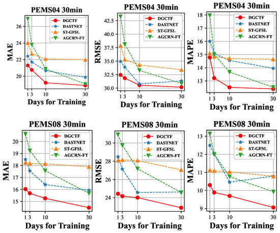
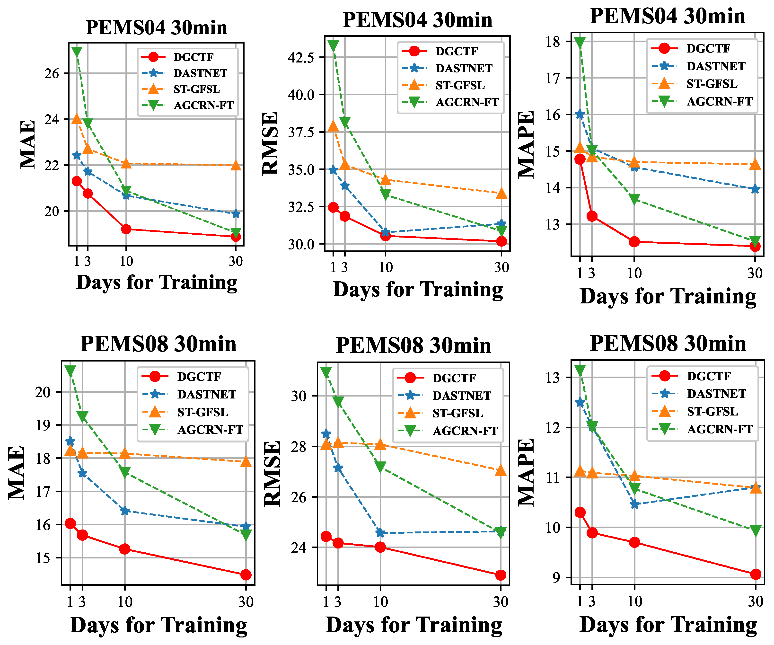
To further explore the robustness of our proposed DGCTF, we conduct experiments on PEMS04 and PEMS08 with different sizes of training sets. We use 1-day, 3-day, 10-day, and 30-day data for training, and use the same amount of test data as in previous experiments for testing. We compare DGCTF with the following transfer learning-based methods: AGCRN-FT, ST-GFSL, and DASTNET. As Figure 5 shows, when the training data are limited (i.e., 1-day and 3-day), these baseline models perform poorly. However, as training data increases, most baseline models show significant improvement. This supports our hypothesis that many existing spatio-temporal prediction methods heavily rely on large training datasets. In contrast, DGCTF consistently outperforms all other models in forecasting future time across different training data sizes. Notably, performance gains over baseline methods are most pronounced in few-shot settings (small training sets). Specifically, the decreases in MAE are 22.30%/18.55%/14.26%/7.65% on PEMS08 for 1/3/10/30 days for training compared with AGCRN-FT and 13.40%10.66%/7.43%/9.10% compared with DASTNET.

Figure 5. Prediction performance under different size of training sets on PEMS04 and PEMS08.

5.7. Parameter Analysis

We also conduct parameter analysis experiments on PEMS04 and PEMS08 to investigate how the key hyper-parameters (the node embedding dimension $d_e$, the functional node representation dimension $d_m$, $T_l$, ${\lambda }_f$ and $\lambda$) in the proposed DGCTF affect the prediction performance.

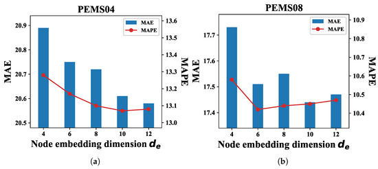
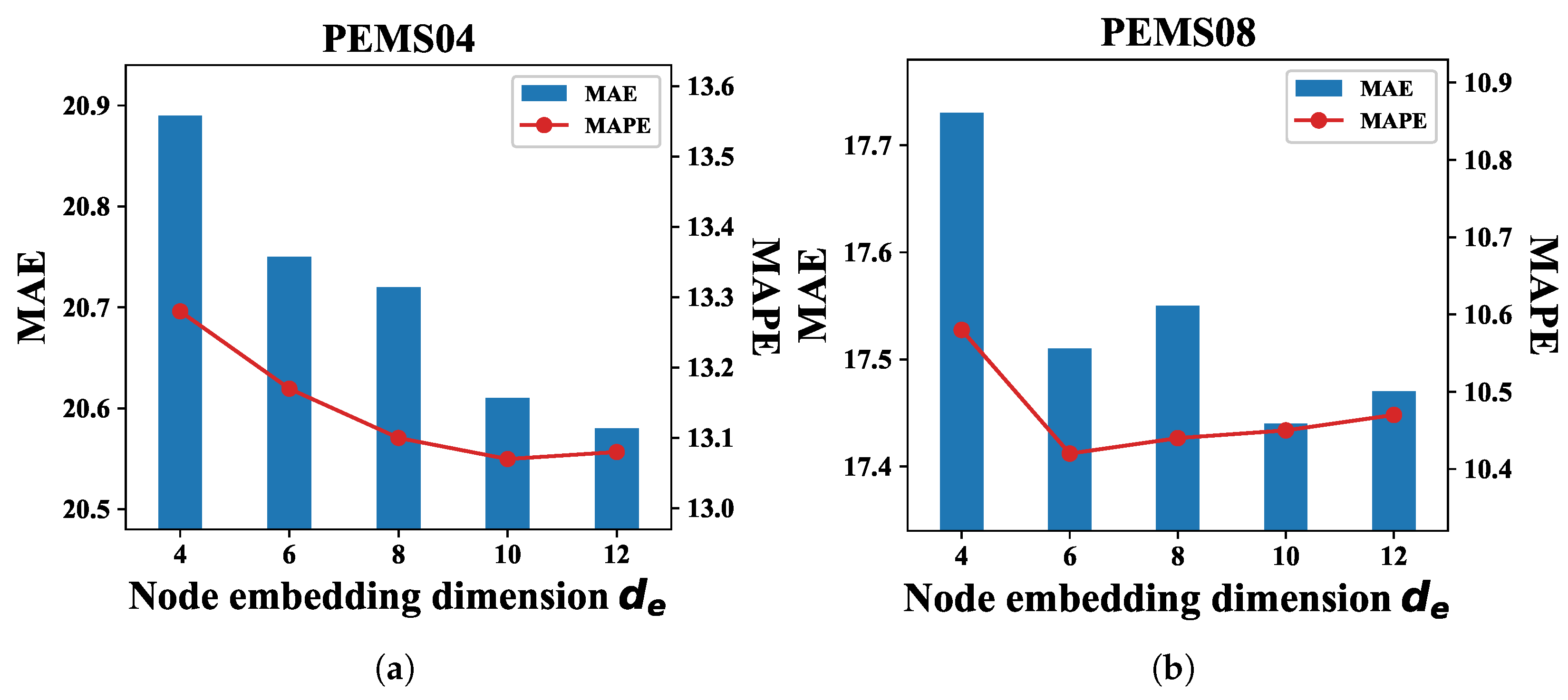
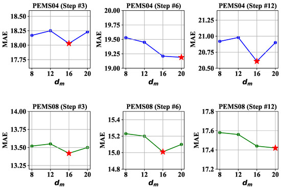
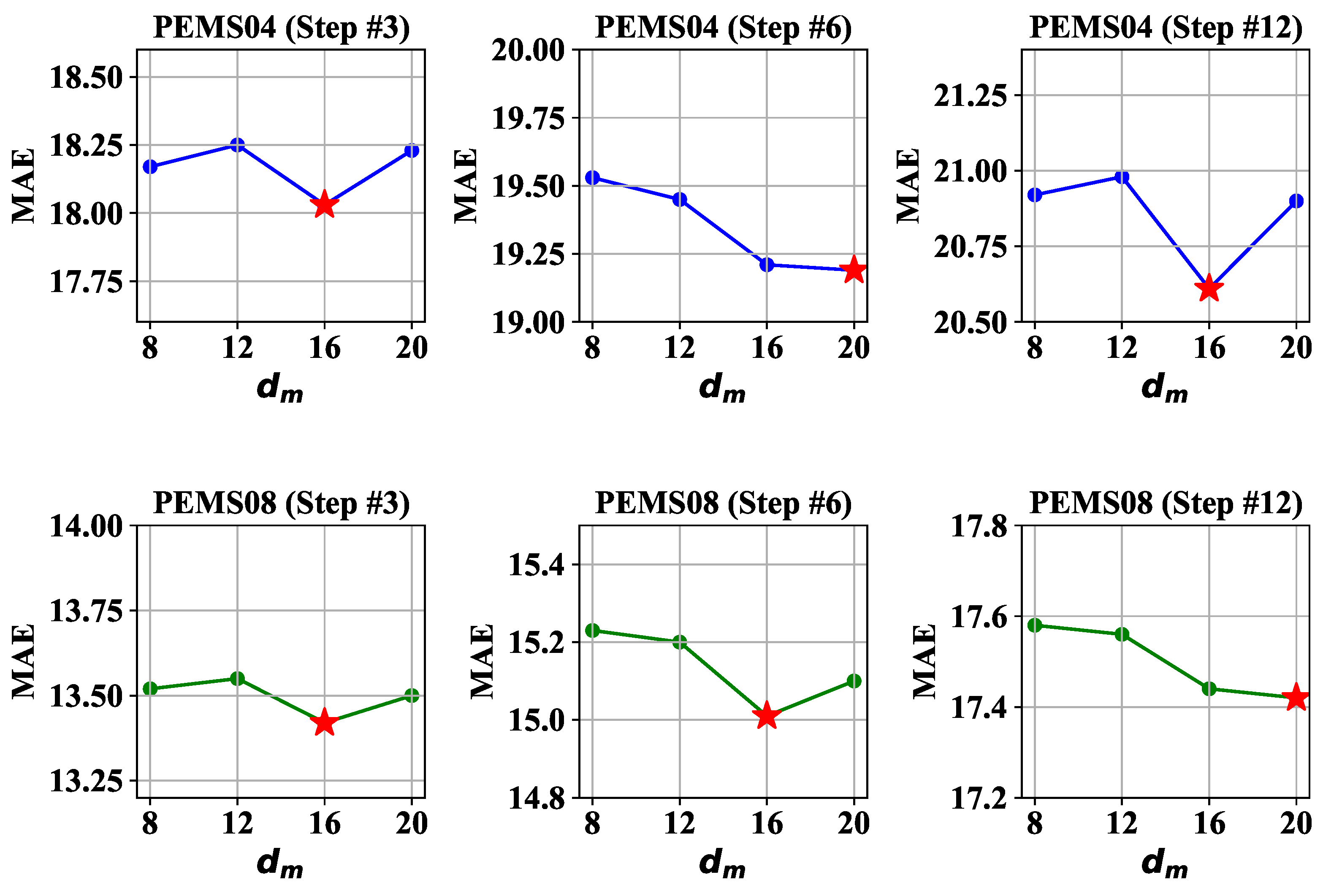
Specifically, we tune $d_e$ in the grid of {4, 6, 8, 10, 12} and tune $d_m$ in the grid of {8, 12, 16, 20}. Figure 6 presents the results for the different node embedding dimensions $d_e$. We can see that smaller $d_e$ fails to capture complex spatio-temporal patterns, while larger values increase computational cost and risk overfitting. For $d_m$, Figure 7 shows that $d_m$ = 16 achieves the best prediction performance across all time steps by balancing expressiveness and efficiency in parameter generation.

Figure 6. Effects of the node embedding dimension $d_e$ on (a) PEMS04 and (b) PEMS08.

Figure 7. Prediction performance under embedding dimension of $d_m$ on PEMS04 and PEMS08. The minimal values of MAE in different steps of PEMS04 and PEMS08 are marked with red stars.

Additionally, we tune $T_l$ in the grid of {1, 3, 6} to investigate the impact of the temporal window size of local attention on the model’s performance. As shown in Table 5, smaller values of $T_l$ fail to capture the necessary short-term temporal features, while larger values overemphasize long-term trends, leading to poorer performance. When $T_l=3$, the model exhibits optimal performance.

Table 5. Effects of $T_l$ on PEMS04 and PEMS08 datasets.

Datasets	${\mathit{T}}_{\mathit{l}}$	MAE	RMSE	MAPE
PEMS04	1	21.32	33.14	13.95
	3	20.61	32.76	13.07
	6	21.11	33.01	13.79
PEMS08	1	17.69	27.78	10.89
	3	17.44	27.36	10.45
	6	17.53	27.77	10.94

Besides, we change ${\lambda }_f$ from 0.1 to 0.7 to explore the trade-off between the two attention, as shown in Table 6, when ${\lambda }_f$ is too large or too small, the model tends to rely excessively on either global or short-term features, neglecting the other type.

Table 6. Effects of ${\lambda }_f$ on PEMS04 and PEMS08 datasets.

Datasets	${\mathit{\lambda }}_{\mathit{f}}$	MAE	RMSE	MAPE
PEMS04	0.1	20.90	32.94	13.64
	0.3	20.83	32.87	13.59
	0.5	20.61	32.76	13.07
	0.7	20.85	32.84	13.61
PEMS08	0.1	17.57	27.54	10.83
	0.3	17.49	27.40	10.77
	0.5	17.44	27.36	10.45
	0.7	17.55	27.41	10.81

Moreover, we change $\lambda$ from 0.1 to 10 to explore the trade-off between the two losses, as shown in Table 7, when $\lambda$ is too small, the impact of CDFAL on the model is limited, leading to suboptimal performance. On the other hand, when $\lambda$ is too large, the model overemphasizes feature alignment, potentially losing focus on the main task. When $\lambda =1$, as it effectively balances the prediction error loss and CDFAL.

Table 7. Effects of $\lambda$ on PEMS04 and PEMS08 datasets.

Datasets	$\mathit{\lambda }$	MAE	RMSE	MAPE
PEMS04	0.1	20.87	32.92	13.66
	1	20.61	32.76	13.07
	5	20.85	32.87	13.63
	10	20.94	32.91	13.71
PEMS08	0.1	17.55	27.49	10.78
	1	17.44	27.36	10.45
	5	17.52	27.42	10.78
	10	17.58	27.49	10.92

Consequently, to balance the performance and cost, we set $d_e$ to 10, and $d_m$ to 16, and $T_l$ to 3, and set ${\lambda }_f$ and $\lambda$ to 0.5, 1 respectively.

5.8. Robustness Analysis

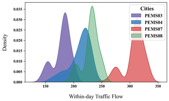
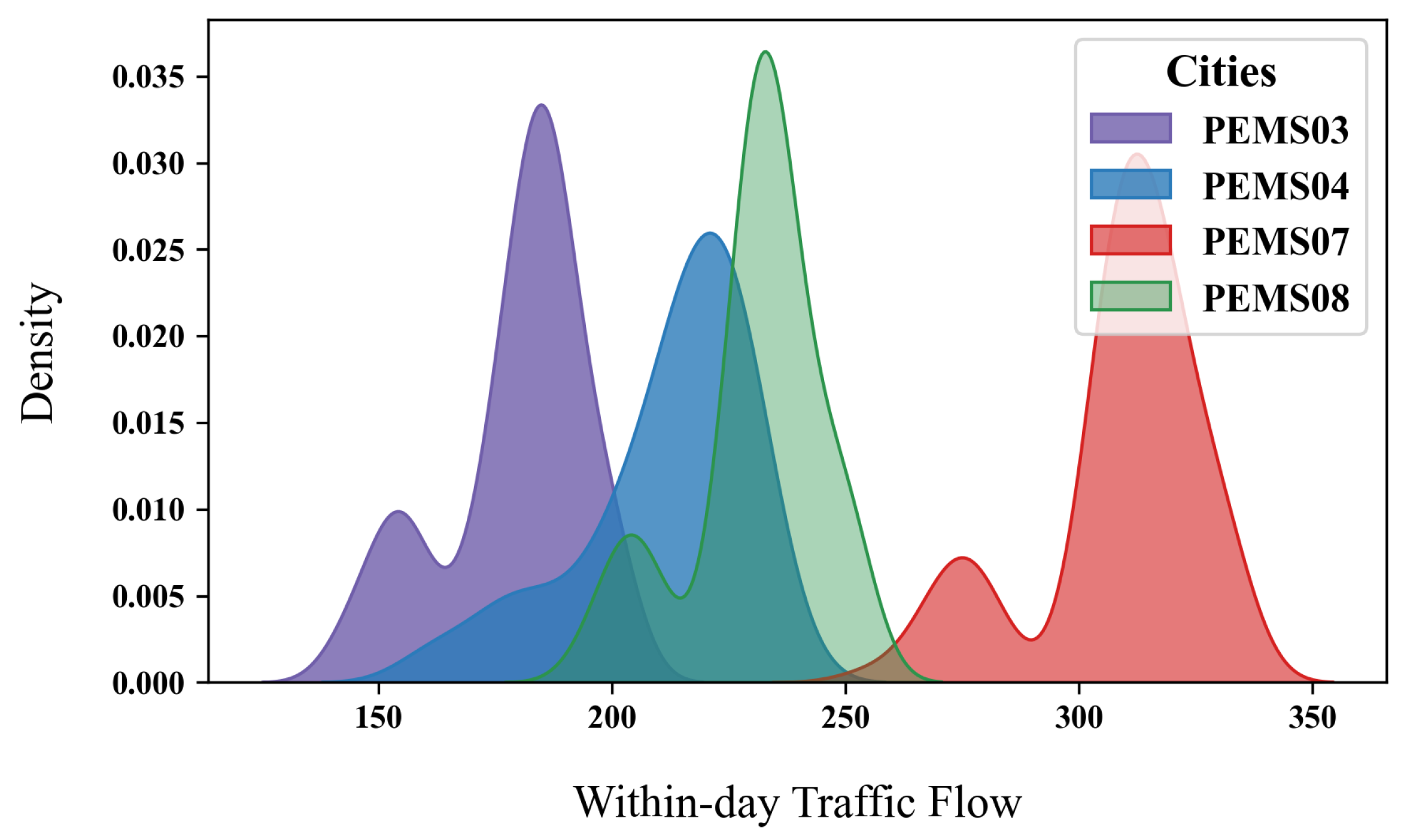
When the source and target domains differ markedly, cross-city knowledge transfer may become less effective and even suffer from negative transfer. To systematically evaluate the robustness of DGCTF under varying distribution shifts, we construct two transfer tasks with the same target city (PEMS08) but different source cities, as shown in Table 8. We measure the source and target discrepancy using MMD in the feature space and visualize the within-day traffic-flow distributions via density curves, as shown in Figure 8. Both the density plots and MMD scores indicate that Task 2 (PEMS03, PEMS07→PEMS08) exhibits a larger distribution gap than Task 1 (PEMS04, PEMS07→PEMS08), and is therefore more challenging.

Table 8. Cross-Domain tasks and corresponding MMD distances.

Task	Source	Target	MMD
Task 1	PEMS04, PEMS07	PEMS08	0.486
Task 2	PEMS03, PEMS07	PEMS08	0.627

Figure 8. Distribution differences across cities.

Table 9 reports the performance of DGCTF and representative transfer-learning baselines on both tasks. As the distribution gap increases from Task 1 to Task 2, most baselines experience a noticeable degradation, whereas DGCTF remains highly stable with only marginal changes in MAE/RMSE/MAPE, demonstrating strong transfer robustness under larger shifts. Moreover, removing CDFAL (DGCTF w/o CL) amplifies the performance drop in Task 2, while the full model consistently mitigates the degradation. This suggests that CDFAL effectively aligns domain-level representations and reduces reliance on source-specific patterns, thereby improving robustness in cross-city transfer.

Table 9. Performance comparison of different transfer-learning models.

Models	Task 1			Task 2			$\mathbf{\Delta }$ Performance (Task 2 vs. Task 1)
	MAE	RMSE	MAPE	MAE	RMSE	MAPE	MAE	RMSE	MAPE
DDGCRN-FT [30]	18.91	30.34	11.50%	19.69	32.17	12.39%	↑ 4.12%	↑ 6.03%	↑ 7.74%
DASTNET [9]	18.84	28.06	11.72%	21.77	33.05	15.80%	↑ 15.55%	↑ 17.78%	↑ 23.02%
TPB [14]	19.41	30.75	12.44%	20.69	32.92	14.21%	↑ 7.99%	↑ 7.06%	↑ 14.23%
DGCTF (proposed)	17.44	27.36	10.45%	17.52	27.55	10.73%	↑ 0.45%	↑ 0.69%	↓ 2.68%
DGCTF w/o CL	17.90	28.02	10.53%	18.27	28.45	10.92%	↑ 2.06%	↑ 1.53%	↓ 3.70%

5.9. Efficiency Analysis

To compare our model with transfer learning baselines, we present the number of tunable parameters and floating-point operations (FLOPs) for forecasting. We set the batch size to 1 and report FLOPs for a single iteration. As shown in Table 10, MTPB incurs the highest computational cost due to its complex multi-module architecture, multi-scale traffic pattern generation, graph reconstruction, and aggregation. ST-GFSL also shows high computational demand as it uses a generator for parameter prediction. In contrast, STGP, achieves the lowest computational demand among the baseline models with its two-stage prompting strategy and task-agnostic architecture. It is worth noting that DGCTF not only surpasses the performance of these baseline methods but also greatly reduces the number of required parameters and FLOPs.

Table 10. Comparison of Tunable Parameters and FLOPs on PEMS08 Dataset.

Method	Parameters	FLOPs $\mathbf{\times }{\mathbf{10}}^{\mathbf{9}}$
DDGCRN-FT [30]	296,242	0.14
ST-GFSL [8]	198,062	8.89
DASTNET [9]	114,331	8.64
TPB [14]	567,110	7.20
MTPB [15]	3,899,852	39.98
STGP [35]	1,248,000	0.33
DGCTF (proposed)	68,410	0.07

6. Conclusions and Future Works

In this paper, we propose a novel framework DGCTF to address the challenges of traffic prediction in data-scarce environments. Our method leverages the similarities in spatio-temporal patterns across different cities to enhance the predictive capabilities of the model. Specifically, DGCTF focuses on capturing the dynamics of traffic networks in cross-domain scenarios. Additionally, we address data discrepancies at multiple granularities, including domain-level and node-level through CDFAL and RGRU-NodePM. These methods effectively mitigate the effects of data distribution differences between cities while achieving node-level personalized adaptation. Through extensive experiments on real-world datasets, we demonstrate that DGCTF consistently outperforms other methods.

However, there is still room for further improvement in DGCTF. For instance, the current model relies primarily on traffic data itself and has not fully taken into account other external factors, such as weather conditions, holidays, and special events, all of which can influence traffic flow. Furthermore, while emergent paradigms like Foundation Models (FM) and Physics-Informed Neural Networks (PINNs) represent prominent frontiers, they were not included in our primary comparison to ensure a rigorous evaluation under equal information constraints. Additionally, as the existing framework is validated exclusively through offline historical datasets, it lacks a direct link to and verification within real-world traffic control scenarios.

Future research could explore how to model these heterogeneous spatio-temporal data to further enhance prediction accuracy. Moreover, inspired by recent advances in large-scale pre-trained architectures, we are also interested in exploring how large language models (LLMs) can be incorporated into the cross-city traffic forecasting pipeline. In addition, we seek to investigate the integration of weak physical priors, such as consistency constraints, together with explicit node-level regularization strategies, to bolster the robustness of the transfer learning process against significant domain discrepancies. Finally, we plan to evaluate the framework within dynamic simulation environments to investigate how DGCTF-based predictions can explicitly inform real-time traffic control strategies and congestion mitigation within active traffic management systems.

References

- Peng, J.; Shangguan, W.; Chai, L.; Chen, J.; Peng, C.; Cai, B. V2X-Enabled Platoon Control for Aperiodic Congestion Mitigation via Moving Bottlenecks in Mixed Traffic Environments. In IEEE Transactions on Vehicular Technology; IEEE: New York, NY, USA, 2025; pp. 1–13. [Google Scholar] [CrossRef] [Scilit]
- Yao, H.; Wu, F.; Ke, J.; Tang, X.; Jia, Y.; Lu, S.; Gong, P.; Ye, J.; Li, Z. Deep multi-view spatial-temporal network for taxi demand prediction. In Proceedings of the 32th AAAI Conference on Artificial Intelligence, New Orleans, LA, USA, 2–7 February 2018; pp. 2588–2595. [Google Scholar]
- Zhou, J.; Cui, G.; Hu, S.; Zhang, Z.; Yang, C.; Liu, Z.; Wang, L.; Li, C.; Sun, M. Graph neural networks: A review of methods and applications. AI Open 2020, 1, 57–81. [Google Scholar] [CrossRef] [Scilit]
- Ouyang, X.; Yang, Y.; Zhou, W.; Zhang, Y.; Wang, H.; Huang, W. Citytrans: Domain-adversarial training with knowledge transfer for spatio-temporal prediction across cities. IEEE Trans. Knowl. Data Eng. 2023, 36, 62–76. [Google Scholar] [CrossRef] [Scilit]
- Jin, Y.; Chen, K.; Yang, Q. Selective cross-city transfer learning for traffic prediction via source city region re-weighting. In Proceedings of the 28th ACM SIGKDD Conference on Knowledge Discovery and Data Mining, Washington, DC, USA, 14–18 August 2022; pp. 731–741. [Google Scholar] [CrossRef] [Scilit]
- Wang, L.; Geng, X.; Ma, X.; Liu, F.; Yang, Q. Cross-city transfer learning for deep spatio-temporal prediction. In Proceedings of the 28th International Joint Conference on Artificial Intelligence, Macao, China, 10–16 August 2019; pp. 1893–1899. [Google Scholar]
- Yao, H.; Liu, Y.; Wei, Y.; Tang, X.; Li, Z. Learning from multiple cities: A meta-learning approach for spatial-temporal prediction. In Proceedings of the World Wide Web Conference, San Francisco, CA, USA, 13–17 May 2019; pp. 2181–2191. [Google Scholar] [CrossRef] [Scilit]
- Lu, B.; Gan, X.; Zhang, W.; Yao, H.; Fu, L.; Wang, X. Spatio-temporal graph few-shot learning with cross-city knowledge transfer. In Proceedings of the 28th ACM SIGKDD Conference on Knowledge Discovery and Data Mining, Washington, DC, USA, 14–18 August 2022; pp. 1162–1172. [Google Scholar] [CrossRef] [Scilit]
- Tang, Y.; Qu, A.; Chow, A.H.; Lam, W.H.; Wong, S.C.; Ma, W. Domain adversarial spatial-temporal network: A transferable framework for short-term traffic forecasting across cities. In Proceedings of the 31st ACM International Conference on Information and Knowledge Management, Atlanta, GA, USA, 17–21 October 2022; pp. 1905–1915. [Google Scholar] [CrossRef] [Scilit]
- Jin, Y.; Chen, K.; Yang, Q. Transferable graph structure learning for graph-based traffic forecasting across cities. In Proceedings of the 29th ACM SIGKDD Conference on Knowledge Discovery and Data Mining, Long Beach, CA, USA, 6–10 August 2023; pp. 1032–1043. [Google Scholar] [CrossRef] [Scilit]
- Xu, Y.; Lu, Y.; Ji, C.; Zhang, Q. Adaptive graph fusion convolutional recurrent network for traffic forecasting. IEEE Internet Things J. 2023, 10, 11465–11475. [Google Scholar] [CrossRef] [Scilit]
- Ji, C.; Xu, Y.; Lu, Y.; Huang, X.; Zhu, Y. Contrastive Learning-Based Adaptive Graph Fusion Convolution Network with Residual-Enhanced Decomposition Strategy for Traffic Flow Forecasting. IEEE Internet Things J. 2024, 11, 20246–20259. [Google Scholar] [CrossRef] [Scilit]
- Ye, J.; Liu, Z.; Du, B.; Sun, L.; Li, W.; Fu, Y.; Xiong, H. Learning the evolutionary and multi-scale graph structure for multivariate time series forecasting. In Proceedings of the 28th ACM SIGKDD Conference on Knowledge Discovery and Data Mining, Washington, DC, USA, 14–18 August 2022; pp. 2296–2306. [Google Scholar] [CrossRef] [Scilit]
- Liu, Z.; Zheng, G.; Yu, Y. Cross-city few-shot traffic forecasting via traffic pattern bank. In Proceedings of the 32st ACM International Conference on Information and Knowledge Management, Birmingham, UK, 21–25 October 2023; pp. 1451–1460. [Google Scholar] [CrossRef] [Scilit]
- Liu, Z.; Zheng, G.; Yu, Y. Multi-scale Traffic Pattern Bank for Cross-city Few-shot Traffic Forecasting. ACM Trans. Knowl. Discov. Data 2025, 19, 1–24. [Google Scholar] [CrossRef] [Scilit]
- Yin, X.; Li, F.; Shen, Y.; Qi, H.; Yin, B. Nodetrans: A graph transfer learning approach for traffic prediction. arXiv 2022, arXiv:2207.01301. [Google Scholar] [CrossRef] [Scilit]
- Yin, X.; Wu, G.; Wei, J.; Shen, Y.; Qi, H.; Yin, B. Deep learning on traffic prediction: Methods, analysis, and future directions. IEEE Trans. Intell. Transp. Syst. 2021, 23, 4927–4943. [Google Scholar] [CrossRef] [Scilit]
- Yu, B.; Yin, H.; Zhu, Z. Spatio-temporal graph convolutional networks: A deep learning framework for traffic forecasting. In Proceedings of the 27th International Joint Conference on Artificial Intelligence, Stockholm, Sweden, 13–19 July 2018; pp. 3634–3640. [Google Scholar]
- Zhao, L.; Song, Y.; Zhang, C.; Liu, Y.; Wang, P.; Lin, T.; Deng, M.; Li, H. T-GCN: A temporal graph convolutional network for traffic prediction. IEEE Trans. Intell. Transp. Syst. 2019, 21, 3848–3858. [Google Scholar] [CrossRef] [Scilit]
- Li, Y.; Yu, R.; Shahabi, C.; Liu, Y. Diffusion convolutional recurrent neural network: Data-driven traffic forecasting. In Proceedings of the 2018 International Conference on Learning Representations, Vancouver, BC, Canada, 30 April–3 May 2018; pp. 1–16. [Google Scholar]
- Wu, Z.; Pan, S.; Long, G.; Jiang, J.; Zhang, C. Graph WaveNet for Deep Spatial-Temporal Graph Modeling. In Proceedings of the 28th International Joint Conference on Artificial Intelligence, Macao, China, 10–16 August 2019; pp. 1907–1913. [Google Scholar]
- Wu, Z.; Pan, S.; Long, G.; Jiang, J.; Chang, X.; Zhang, C. Connecting the dots: Multivariate time series forecasting with graph neural networks. In Proceedings of the 26th ACM SIGKDD Conference on Knowledge Discovery and Data Mining, Virtual Event, 23–27 August 2020; pp. 753–763. [Google Scholar] [CrossRef] [Scilit]
- Bai, L.; Yao, L.; Li, C.; Wang, X.; Wang, C. Adaptive graph convolutional recurrent network for traffic forecasting. Adv. Neural Inf. Process. Syst. 2020, 33, 17804–17815. [Google Scholar]
- Liu, H.; Zhu, C.; Zhang, D.; Li, Q. Attention-based spatial-temporal graph convolutional recurrent networks for traffic forecasting. In Proceedings of the Advanced Data Mining and Applications, Shenyang, China, 21–23 August 2023; pp. 630–645. [Google Scholar]
- Fang, Z.; Long, Q.; Song, G.; Xie, K. Spatial-temporal graph ode networks for traffic flow forecasting. In Proceedings of the 27th ACM SIGKDD Conference on Knowledge Discovery and Data Mining, Virtual Event, 14–18 August 2021; pp. 364–373. [Google Scholar] [CrossRef] [Scilit]
- Zhang, X.; Huang, C.; Xu, Y.; Xia, L.; Dai, P.; Bo, L.; Zhang, J.; Zheng, Y. Traffic flow forecasting with spatial-temporal graph diffusion network. In Proceedings of the 35th AAAI Conference on Artificial Intelligence, Virtually, 19–21 May 2021; pp. 15008–15015. [Google Scholar]
- Lan, S.; Ma, Y.; Huang, W.; Wang, W.; Yang, H.; Li, P. Dstagnn: Dynamic spatial-temporal aware graph neural network for traffic flow forecasting. In Proceedings of the 39th International Conference on Machine Learning, Baltimore, MD, USA, 17–23 July 2022; pp. 11906–11917. [Google Scholar]
- Zhao, Y.; Luo, X.; Ju, W.; Chen, C.; Hua, X.S.; Zhang, M. Dynamic hypergraph structure learning for traffic flow forecasting. In Proceedings of the 2023 IEEE 39th International Conference on Data Engineering, Anaheim, CA, USA, 3–7 April 2023; pp. 2303–2316. [Google Scholar]
- Li, R.; Zhang, F.; Li, T.; Zhang, N.; Zhang, T. DMGAN: Dynamic multi-hop graph attention network for traffic forecasting. IEEE Trans. Knowl. Data Eng. 2022, 35, 9088–9101. [Google Scholar] [CrossRef] [Scilit]
- Weng, W.; Fan, J.; Wu, H.; Hu, Y.; Tian, H.; Zhu, F.; Wu, J. A decomposition dynamic graph convolutional recurrent network for traffic forecasting. Pattern Recognit. 2023, 142, 109670. [Google Scholar] [CrossRef] [Scilit]
- Tian, C.; Zhu, X.; Hu, Z.; Ma, J. A transfer approach with attention reptile method and long-term generation mechanism for few-shot traffic prediction. Neurocomputing 2021, 452, 15–27. [Google Scholar] [CrossRef] [Scilit]
- Wang, S.; Miao, H.; Li, J.; Cao, J. Spatio-temporal knowledge transfer for urban crowd flow prediction via deep attentive adaptation networks. IEEE Trans. Intell. Transp. Syst. 2021, 23, 4695–4705. [Google Scholar] [CrossRef] [Scilit]
- Fang, Z.; Wu, D.; Pan, L.; Chen, L.; Gao, Y. When Transfer Learning Meets Cross-City Urban Flow Prediction: Spatio-Temporal Adaptation Matters. In Proceedings of the 31st International Joint Conference on Artificial Intelligence, Vienna, Austria, 23–29 July 2022; Volume 22, pp. 2030–2036. [Google Scholar]
- Yao, Z.; Xia, S.; Li, Y.; Wu, G.; Zuo, L. Transfer learning with spatial–temporal graph convolutional network for traffic prediction. IEEE Trans. Intell. Transp. Syst. 2023, 24, 8592–8605. [Google Scholar] [CrossRef] [Scilit]
- Hu, J.; Liu, X.; Fan, Z.; Yin, Y.; Xiang, S.; Ramasamy, S.; Zimmermann, R. Prompt-Based Spatio-Temporal Graph Transfer Learning. In Proceedings of the 33rd ACM International Conference on Information and Knowledge Management, Boise, ID, USA, 21–25 October 2024. [Google Scholar] [CrossRef] [Scilit]
- Ouyang, X.; Yang, Y.; Zhang, Y.; Zhou, W.; Wan, J.; Du, S. Domain adversarial graph neural network with cross-city graph structure learning for traffic prediction. Knowl.-Based Syst. 2023, 278, 110885. [Google Scholar] [CrossRef] [Scilit]
- Finn, C.; Abbeel, P.; Levine, S. Model-agnostic meta-learning for fast adaptation of deep networks. In Proceedings of the 34th International Conference on Machine Learning, Sydney, Australia, 6–11 August 2017; pp. 1126–1135. [Google Scholar]
- Shao, Z.; Zhang, Z.; Wang, F.; Xu, Y. Pre-training Enhanced Spatial-temporal Graph Neural Network for Multivariate Time Series Forecasting. In Proceedings of the 28th ACM SIGKDD Conference on Knowledge Discovery and Data Mining, Washington, DC, USA, 14–18 August 2022; pp. 1567–1577. [Google Scholar] [CrossRef] [Scilit]
- Yu, H.; Li, T.; Yu, W.; Li, J.; Huang, Y.; Wang, L.; Liu, A. Regularized Graph Structure Learning with Semantic Knowledge for Multi-variates Time-Series Forecasting. In Proceedings of the 31th International Joint Conference on Artificial Intelligence, Vienna, Austria, 23–29 July 2022; pp. 2362–2368. [Google Scholar]
- Sun, B.; Saenko, K. Deep CORAL: Correlation Alignment for Deep Domain Adaptation. In Proceedings of the 14th European Conference on Computer Vision, Amsterdam, The Netherlands, 8–16 October 2016; pp. 443–450. [Google Scholar]
- Tian, C.; Chan, W.K.V. Spatial-temporal attention wavenet: A deep learning framework for traffic prediction considering spatial-temporal dependencies. IET Intell. Transp. Syst. 2021, 15, 549–561. [Google Scholar] [CrossRef] [Scilit]
- Vettoruzzo, A.; Bouguelia, M.R.; Rögnvaldsson, T. Meta-learning for efficient unsupervised domain adaptation. Neurocomputing 2024, 574, 127264. [Google Scholar] [CrossRef] [Scilit]
- Chen, C.; Petty, K.; Skabardonis, A.; Varaiya, P.; Jia, Z. Freeway performance measurement system: Mining loop detector data. Transp. Res. Rec. 2001, 1748, 96–102. [Google Scholar] [CrossRef] [Scilit]
- Didi-Chuxing. Didi Chuxing Gaia Initiative. 2020. Available online: https://gaia.didichuxing.com (accessed on 14 February 2020).
- Liu, J.; Guan, W. A summary of traffic flow forecasting methods. J. Highway Transp. Res. Dev. 2004, 21, 82–85. [Google Scholar]
- Cho, K.; van Merriënboer, B.; Bahdanau, D.; Bengio, Y. On the Properties of Neural Machine Translation: Encoder–Decoder Approaches. In Proceedings of the 8th Workshop on Syntax, Semantics and Structure in Statistical Translation, Doha, Qatar, 25 October 2014; pp. 103–111. [Google Scholar]
- Kipf, T.N.; Welling, M. Semi-Supervised Classification with Graph Convolutional Networks. In Proceedings of the 2017 International Conference on Learning Representations, Toulon, France, 24–26 April 2017; pp. 1–14. [Google Scholar]
- Wang, S.; Wu, H.; Shi, X.; Hu, T.; Luo, H.; Ma, L.; Zhang, J.Y.; Zhou, J. Timemixer: Decomposable multiscale mixing for time series forecasting. In Proceedings of the 2024 International Conference on Learning Representations, Vienna Austria, 7–11 May 2024. [Google Scholar]
- Zhang, Z.; Cheng, Q.; Li, Z.; Fang, Y.; Li, Y. MC-HSTA: A multi-source cross-domain hybrid spatio-temporal attention network for traffic flow prediction. Neural Netw. 2026, 196, 108358. [Google Scholar] [CrossRef] [Scilit] [PubMed]
Disclaimer/Publisher’s Note: The statements, opinions and data contained in all publications are solely those of the individual author(s) and contributor(s) and not of MDPI and/or the editor(s). MDPI and/or the editor(s) disclaim responsibility for any injury to people or property resulting from any ideas, methods, instructions or products referred to in the content. |
© 2026 by the authors. Licensee MDPI, Basel, Switzerland. This article is an open access article distributed under the terms and conditions of the Creative Commons Attribution (CC BY) license.