Low Carbon Economic Dispatch of IES Considering Flexibility and Multi-Entity Participation Based on Improved PSO

Abstract

To address the significant scheduling challenges arising from high-penetration renewable integration and coupled multi-energy loads, this study examines the operational scheduling of an integrated energy system (IES) that incorporates system operators, user aggregators, electric vehicles, and other stakeholders. First, the flexibility demand and supply resources in the IES were analyzed, and flexibility indicators were quantified. Subsequently, a multi-objective bi-level optimization model considering flexibility and multi-entity participation was established for the IES’s low-carbon economic dispatch. The upper-level model considered the IES operator’s revenue and system flexibility, incorporating a green certificate carbon trading mechanism, while the lower-level model accounted for user aggregator costs and electric vehicle self-benefits, with interactions between the two levels through energy prices and purchase quantities. Finally, an improved Particle Swarm Optimization (PSO) algorithm was employed to solve the proposed upper-level model, and CPLEX 12.10 software was used for the lower-level model. A typical scenario in northern China was selected to validate the proposed model. The results demonstrated that the proposed model balanced system economy and flexibility compared to the traditional single-objective economic dispatch. Compared with only considering the benefits of operators, the proposed model can balance the interests of multiple parties. Additionally, compared to the traditional PSO algorithm, the improved PSO algorithm reduced the number of iterations at convergence by 52.0%, improved the closeness of the obtained optimal solution to the ideal solution by 7.5%, and had better convergence and optimization performance.

1. Introduction

Compared to traditional separate energy systems, integrated energy systems consider the production, transmission, conversion, and consumption of different energy forms (electricity, heat, gas, cooling, etc.) in a unified manner, offering significant advantages such as higher flexibility and better complementarity. As an integral mechanism for energy conservation, emission reduction, and improved energy utilization efficiency, integrated energy systems provide robust support for achieving the “Dual Carbon” goals [1,2]. In [3], the stepped carbon trading cost is incorporated within the carbon emission framework, with case studies demonstrating that the stepped carbon trading mechanism further reduces carbon emissions compared to the traditional Carbon Emissions Trading (CET) mechanism. In [4], Fan examines how carbon quota and trading policies affect carbon emissions, demonstrating that appropriately calibrated institutional coefficients in the carbon trading mechanism can lead to a win–win outcome for both economic efficiency and low-carbon sustainability. In [5], an integrated scheduling model combining green certificate trading (GCT) and carbon trading is proposed. The inherent synergy and convertibility between these two mechanisms drive higher renewable energy accommodation and lower carbon emissions. Li [6] established a low-carbon scheduling model for IES incorporating wind power, PV, and hydrogen storage. By introducing P2G technology and carbon capture equipment to achieve multi-energy coupling, the model effectively enhances the accommodation of wind and PV power while promoting deep decarbonization of the system. Yang [7] proposed an optimization scheduling model for low-carbon community IES considering resource flexibility and segmented control of solid oxide fuel cells. The proposed method effectively promoted low-carbon economic operation of the system by mobilizing different types of energy storage equipment and load-side flexible resources. A novel modular distributed framework, introduced in [8], serves as a key solution for unlocking greater flexibility and enhanced profitability in nuclear-renewable hybrid energy systems.

However, as the proportion of renewable energy increases, its output uncertainty amplifies the difficulty of system regulation [9]. Concurrently, fluctuations on the load side increase supply–demand uncertainty. This presents a substantial challenge to the secure and stable operation of IES, thereby necessitating enhanced flexible regulation capacities. In [10], IES flexibility is defined as the system’s ability to regulate energy supply, demand, and power flows effectively within a designated area while ensuring stable operation. Flexibility resources are the prerequisite for system flexibility. In [11], flexibility resources are defined as adjustable generating units, energy storage devices, responsive flexible loads, electric vehicles, and other resources within the power system. Demand response, as a critical measure for regulating load power and promoting supply–demand balance, additionally plays a significant role in enhancing system flexibility [12]. In [13], a multi-objective optimization model simultaneously considering electricity and gas demand response is established. The objective functions include the economic cost of the IES and user satisfaction, effectively reducing end-user load fluctuations and enhancing load-shifting efficiency. In [14], the enhancement effect of multiple flexibility resources on overall system flexibility is analyzed; fully leveraging and integrating diverse flexibility resources boosts wind power accommodation and reduces carbon emissions. To address system flexibility demands, reference [15] quantifies demands via segmented renewable outputs. Similarly, a multi-agent deep reinforcement learning-based strategy for distributed energy hubs is proposed to enable safe scheduling under carbon trading costs while protecting sensitive data through differential privacy. This approach enhances operational flexibility by coordinating hydrogen, gas, and storage resources in a decentralized manner [16]. In [17], a low-carbon economic scheduling framework for multi-microgrids is introduced. By minimizing both operating cost and carbon emissions, this work demonstrated the potential of advanced learning-based strategies to improve flexibility and sustainability. Arvanitidis [18] focused on a novel nuclear integrated energy system configuration that combines small modular reactors, renewable energy sources, energy storage, and a thermal network coupled with the IEEE-30 Bus system for security-constrained economic dispatch. By integrating nuclear base load generation with intermittent RES, the approach enhanced operational flexibility and efficiency in complex energy configurations.

Electric vehicles (EVs) serve as flexibility resources, offering new possibilities for optimizing demand response and electricity markets. In [19], a two-stage optimization strategy for EV charging and discharging based on the PSO algorithm is proposed. This strategy comprehensively considers EV charging demands and grid operational conditions, optimizing EV charging behavior through demand response mechanisms. It enhances grid stability and improves economic benefits for EV users. In [20], the flexibility of large-scale electric buses is quantified, effectively evaluating both their upward and downward flexibility. Additionally, it demonstrates the potential for fleet operators to generate additional economic revenue by providing such flexibility to the flexibility market.

An integrated energy system is a comprehensive platform that spans energy production, transmission, and consumption, involving multiple stakeholders such as system operators and end-users. In [21], power grids and gas networks are treated as distinct entities, with game-theoretic interactions between them fully considered to balance their interests. In [22], a Stackelberg game-based IES scheduling optimization framework is established to reconcile interests between IES operators and users, effectively coordinating their relationship. A non-cooperative game and multi-energy pricing strategy is employed in [23] for IES demand-side management. The results demonstrate successful coordinated optimization between users and suppliers, leading to reduced peak–valley load ratios and lower energy costs. In [24], a virtual power plant optimization configuration method considering multi-entity participation of electric vehicles and load aggregators is proposed; through this coordinated mechanism, enhanced operational sustainability with improved power supply reliability, reduced charging disorderliness, and low-carbon economic operation is achieved.

To solve the scheduling model, various methods have been employed. In [25], an IES optimization operation model incorporating stochastic robust optimization for electric vehicles and the participation of user aggregators is established. By considering the uncertainty of EV charging behaviors and user demand response, this model optimizes the economic operation of IES, reduces economic losses for users, and lowers the system’s total operational costs. In [26], a bi-level game dispatch model is proposed for the park integrated energy system (PIES), where the synergy of electricity-carbon market decision-making is explicitly considered. The improved alternating direction method of multipliers (ADMM) is used to solve the distributed optimization problem. Liu [27] constructs a hybrid game architecture with the energy system operator as the main body and the RIES alliance as the slave, and the hybrid game process is solved using Genetic Algorithm. The Particle Swarm Optimization (PSO) algorithm is well-suited for solving the optimal scheduling problem of an IES due to its concise implementation and fast convergence [28]. However, the scheduling model itself presents a significant challenge, as it is a nonlinear problem characterized by numerous constraints and a complex objective function. The scheduling problem of IES contains many equality constraints relating to the balance of IES, which makes the particles fall into the local optimal solution easily during the iterative process, and thus cannot obtain the proper optimal solution.

In summary, research on integrated energy system optimization scheduling has achieved notable advancements in model development, providing diverse operational solutions for such systems. However, existing studies primarily emphasize economic optimization among multiple entities while overlooking flexibility objectives; alternatively, they consider flexibility objectives but tend to prioritize the interests of a single participant. In response to this issue, a low-carbon optimization model is established in this work, which explicitly accounts for flexibility requirements and multi-entity involvement, thereby achieving a trade-off between economic efficiency and system flexibility. An improved Particle Swarm Optimization algorithm is applied to solve the multi-objective optimization model, which helps to prevent convergence to local optima.

In contrast to the existing literature, this work offers the following original contributions:

(1)

The flexibility resources on both the supply and demand sides are fully utilized, and the calculation formula for flexibility evaluation indicators is provided.

(2)

With the objectives of economy and flexibility, a two-layer optimization model for IES economic dispatch considering multi-entity participation is established to balance multiple operational objectives and effectively reconcile stakeholders’ interests.

(3)

An improved PSO algorithm with adaptive weights, optimized learning factors and distinct position updated formulas is employed to reduce the probability of particles falling into local optimal solution, demonstrating superior convergence and optimization performance compared to traditional PSO algorithm.

The research is structured as follows: first, it gives a review of the current research and research gap, followed by the proposal of quantitative indicators for flexibility. Subsequently, a low-carbon economic dispatch model for integrated energy systems (IESs) is established, incorporating both flexibility considerations and multi-entity participation. Finally, an improved Particle Swarm Optimization algorithm is employed to solve the model, verifying its validity and feasibility.

2. IES Flexibility Indicators

2.1. Flexibility Demand Situation

The flexibility demand of IES mainly originates from the volatility and uncertainty of wind energy, solar energy, and load. In addition, the anti-peak shaving characteristics of wind and solar power output may cause the net load curve to fluctuate in the opposite trend to the load curve.

The relationship between net load and flexibility resource output usually falls into three scenarios: When the net load fluctuation exceeds the upper limit of flexibility resource output, the system cannot meet the upward flexibility demand, which may lead to energy supply interruption or unstable system operation. When the net load remains between the upper and lower limits of flexibility resource output, the system can better meet the flexibility demand and achieve supply–demand balance. When the net load fluctuation is lower than the lower limit of flexibility resource output, the system faces the inability to meet the downward flexibility demand, resulting in resource surplus, which may cause waste of idle resources and economic losses.

According to the directional characteristics of flexibility, the upward and downward flexibility demands of IES can be expressed by the following equations:

$$\left\{\begin{array}{l}{P}_{\mathrm{u}}^t=\max (P_{\mathrm{NL}}^{t+1}-P_{\mathrm{NL}}^t,0)\\ P_{\mathrm{d}}^t=-\min (P_{\mathrm{NL}}^{t+1}-P_{\mathrm{NL}}^t,0)\end{array}\right.$$

(1)

where $P_{\mathrm{u}}^t$ and $P_{\mathrm{d}}^t$ are the upward and downward flexibility demands of IES at time t; $P_{\mathrm{NL}}^{t+1}$ and $P_{\mathrm{NL}}^t$ are the net loads at time t + 1 and t, respectively.

2.2. Flexibility Supply Situation

Flexibility resources on the source and energy storage sides have the characteristics of convenient control and flexible scheduling. As a special flexibility resource, demand response on the load side provides new ideas and strategies for IES. This demand response mechanism improves the operation efficiency and flexibility of the entire IES by incentivizing users to adjust their power consumption behavior.

1.

Flexibility Supply of Energy Conversion Equipment

The energy conversion equipment contributes an electrical flexibility margin, which is given by:

$$\left\{\begin{array}{l}{S}_{\mathrm{u}}^t={\displaystyle \sum _{j=1}^N\min \left(P^{\max }-P^t,R^{\mathrm{up}}\right)}\\ S_{\mathrm{d}}^t={\displaystyle \sum _{j=1}^N\min \left(P^t-P^{\min },R^{\mathrm{down}}\right)}\end{array}\right.$$

(2)

where $S_{\mathrm{u}}^t$ and $S_{\mathrm{d}}^t$ are the upward and downward flexibility margins provided by energy conversion equipment at time t; $P^{\max }$ and $P^{\min }$ are the upper and lower power limits of the equipment; $P^t$ is the actual power output at time t; $R^{\mathrm{up}}$ and $R^{\mathrm{down}}$ are the upward and downward ramping rates, respectively.

2.

Flexibility Supply of Energy Storage Equipment

Energy storage equipment supplies a flexibility margin, calculated as:

$$\left\{\begin{array}{l}{S}_{\mathrm{u}}^{S,t}=\min \left({\eta }_{\mathrm{chr}}\left(S_{\mathrm{BT}}^t-S^{\min }\right),P_{\mathrm{chr}}^{\max }\right)\\ S_{\mathrm{d}}^{S,t}=\min \left({\eta }_{\mathrm{dis}}\left(S^{\max }-S_{\mathrm{BT}}^t\right),P_{\mathrm{dis}}^{\max }\right)\end{array}\right.$$

(3)

where $S_{\mathrm{u}}^{S,t}$ and $S_{\mathrm{d}}^{S,t}$ are the upward and downward flexibility margins provided by energy storage equipment at time t; $S_{\mathrm{BT}}^t$ is the remaining capacity of the energy storage device at time t; ${\eta }_{\mathrm{chr}}$ and ${\eta }_{\mathrm{dis}}$ are the charging and discharging efficiencies; $P_{\mathrm{chr}}$ and $P_{\mathrm{dis}}$ are the charging and discharging powers; $S^{\max }$ and $S^{\min }$ are the upper and lower limits of energy storage capacity, respectively.

3.

Flexibility Supply of Load Demand Response

The flexibility margin from load demand response is determined by its adjustable capacity and the system operating status, expressed as:

$$\left\{\begin{array}{l}{S}_{\mathrm{u}}^{L,t}=P_{\mathrm{cut}}^{t.\max }-P_{\mathrm{cut}}^t+P_{\mathrm{out}}^{t.\max }-P_{\mathrm{out}}^t\\ S_{\mathrm{d}}^{L,t}=P_{\mathrm{in}}^{t.\max }-P_{\mathrm{in}}^t\end{array}\right.$$

(4)

where $S_{\mathrm{u}}^{L,t}$, $S_{\mathrm{d}}^{L,t}$ are the upward/downward flexibility margins provided by load demand response at time t; $P_{\mathrm{cut}}^t$, $P_{\mathrm{out}}^t$, and $P_{\mathrm{in}}^t$ are the reducible load, transferred-out load, and transferred-in load at time t, respectively; accordingly, $P_{\mathrm{cut}}^{t.\max }$, $P_{\mathrm{out}}^{t.\max }$, and $P_{\mathrm{in}}^{t.\max }$ are the maximum values.

In summary, the upward flexibility $F_{\mathrm{u}}^t$ and downward flexibility $F_{\mathrm{d}}^t$ of the supply of flexibility resources at time t are as shown in the following formula.

$$\left\{\begin{array}{l}{F}_{\mathrm{u}}^t=S_{\mathrm{u}}^t+S_{\mathrm{u}}^{\mathrm{S},t}+S_{\mathrm{u}}^{\mathrm{L},t}\\ F_{\mathrm{d}}^t=S_{\mathrm{d}}^t+S_{\mathrm{d}}^{\mathrm{S},t}+S_{\mathrm{d}}^{\mathrm{L},t}\end{array}\right.$$

(5)

2.3. Flexibility Evaluation Indicators

To more accurately evaluate the flexibility of the system, it is necessary to establish flexibility evaluation indicators. Its physical significance lies in measuring the response capability of the IES to net load fluctuations. A larger indicator value indicates that the system has more sufficient flexibility and stronger adaptability to load fluctuations.

The flexibility evaluation indicator is expressed as follows:

$$\left\{\begin{array}{c}{F}_{\mathrm{e}}={\displaystyle \frac{F_{\mathrm{u}}^{\mathrm{e}}+F_{\mathrm{d}}^{\mathrm{e}}}{2P_L^{\mathrm{e}}}}\\ F_h={\displaystyle \frac{F_{\mathrm{u}}^{\mathrm{h}}+F_{\mathrm{d}}^{\mathrm{h}}}{2P_L^{\mathrm{h}}}}\\ F_{\mathrm{q}}={\displaystyle \frac{F_{\mathrm{u}}^{\mathrm{q}}+F_{\mathrm{d}}^{\mathrm{q}}}{2P_L^{\mathrm{q}}}}\end{array}\right.$$

(6)

where $F_{\mathrm{e}}$, $F_{\mathrm{h}}$ and $F_{\mathrm{q}}$ are flexibility evaluation indicators of electrical energy, thermal energy, and cooling energy; accordingly $F_{\mathrm{u}}^{\mathrm{e}}$, $F_{\mathrm{u}}^{\mathrm{h}}$ and $F_{\mathrm{u}}^{\mathrm{q}}$ are the upward flexibility supplies; $F_{\mathrm{d}}^{\mathrm{e}}$, $F_{\mathrm{d}}^{\mathrm{h}}$ and $F_{\mathrm{d}}^{\mathrm{q}}$ are the downward flexibility supplies; $P_{\mathrm{L}}^{\mathrm{e}}$, $P_{\mathrm{L}}^{\mathrm{h}}$ and $P_{\mathrm{L}}^{\mathrm{q}}$ are the power supplied to the IES.

3. Dispatch Model for IES Considering Flexibility and Multi-Entity Participation

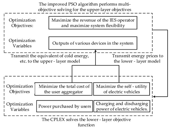
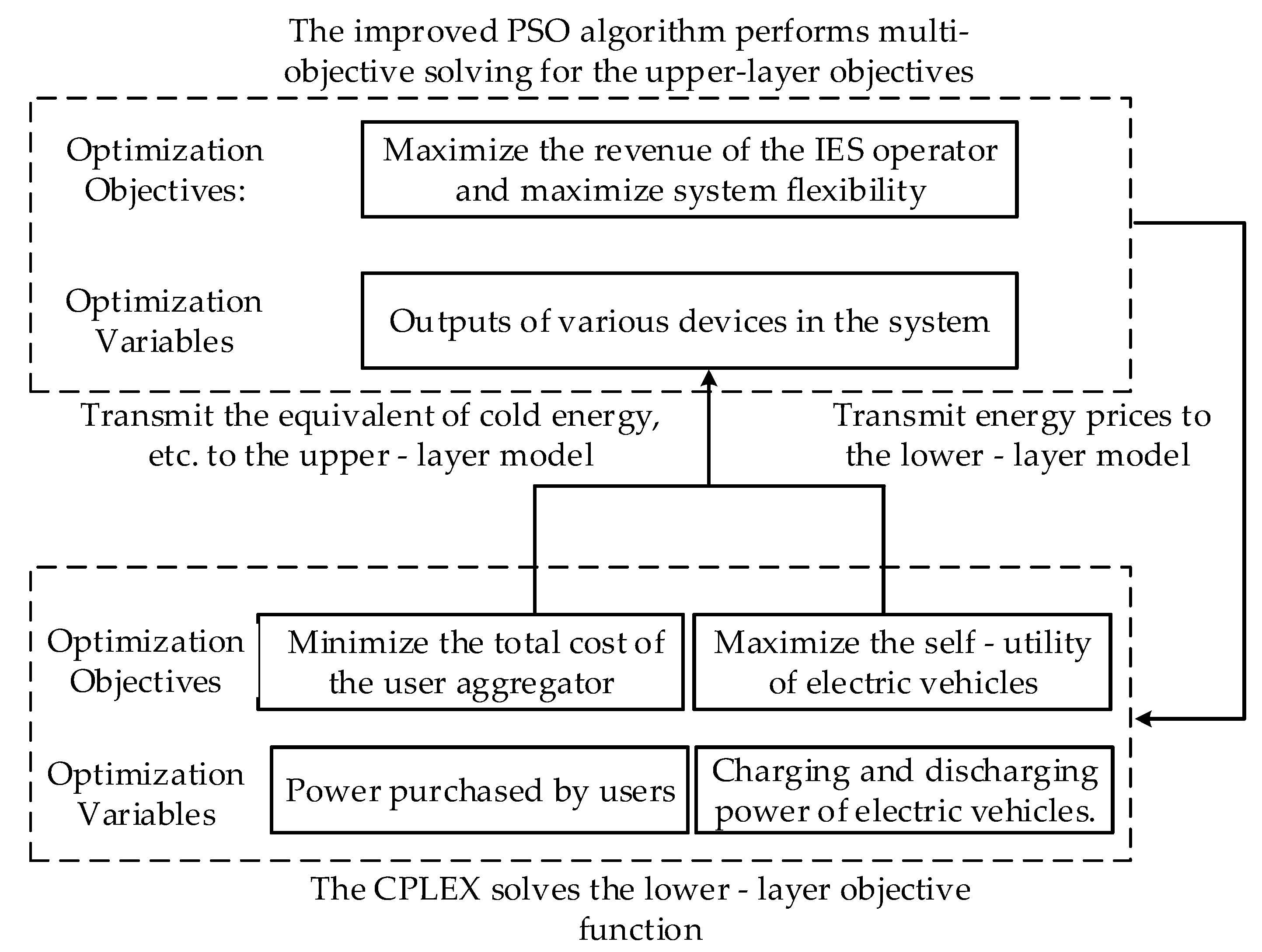
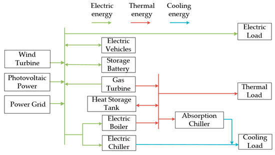
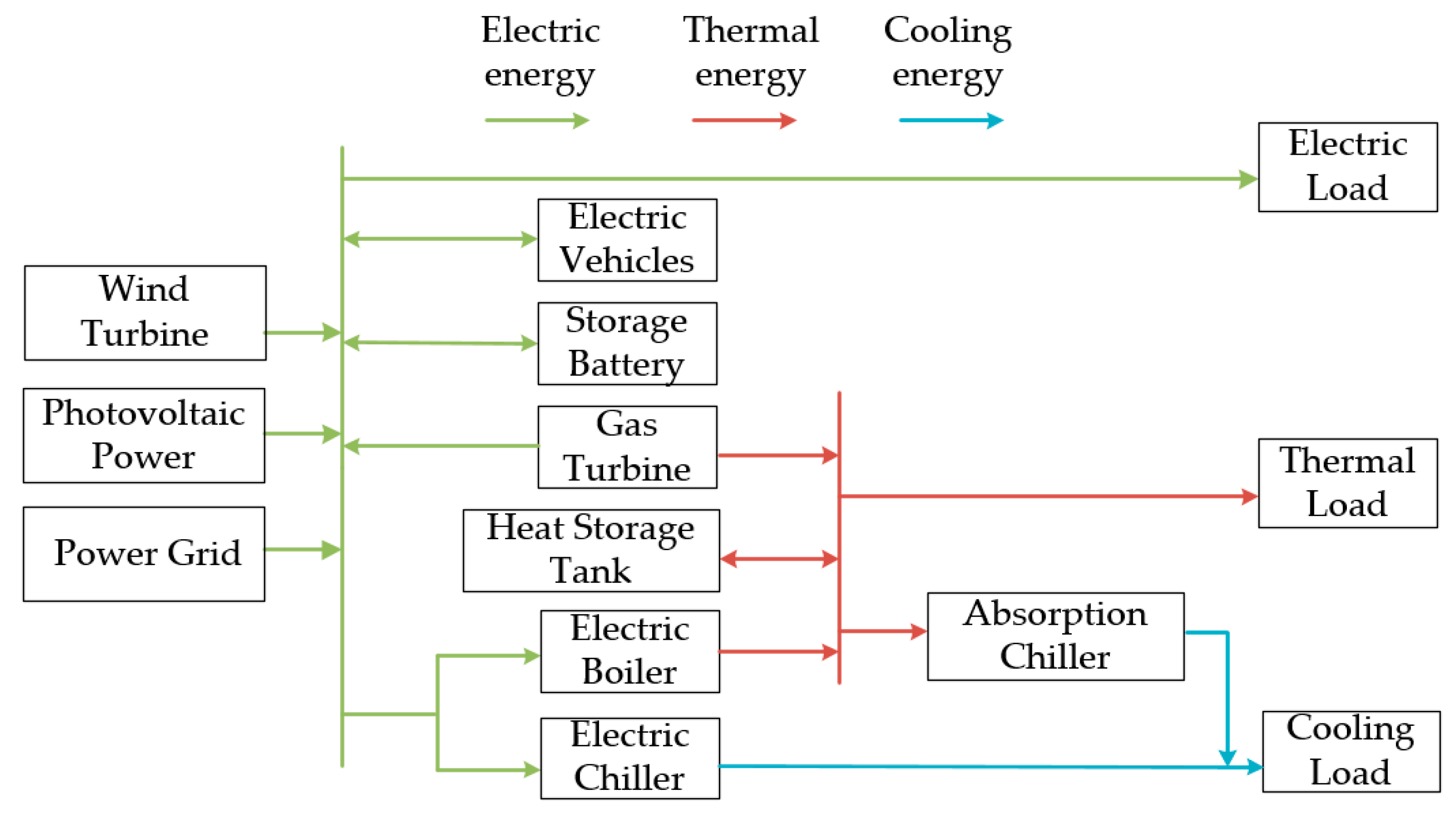
Against the backdrop of steady power market reforms, a new competitive landscape has evolved, marked by the participation of multiple entities such as IES operators and competition among diverse market elements. This paper develops a bi-layer optimal dispatch model featuring multi-entity participation. The upper layer optimizes IES operator revenue and system flexibility while incorporating the GCT-CET mechanism; the lower layer accounts for user aggregator costs and the individual benefits of EVs. As the upper-layer leader, the IES operator can give priority to releasing price strategies for electric energy, thermal energy, and cooling energy; user aggregators and electric vehicles, as lower-layer participants, can implement more reasonable demand response strategies and charging–discharging plans according to changes in energy prices to ensure the optimization of their own goals, and at the same time, promptly feed back their own energy usage adjustments to the IES operator. The two-layer optimization model is shown in Figure 1, and the IES structure diagram is shown in Figure 2.

Figure 1. A two-layer model considering multi-entity participation in IES optimization.

Figure 2. IES structure diagram.

3.1. Upper-Layer Model

3.1.1. Objective Function

The upper-layer objective function includes the economic objective and the flexibility objective of the IES operator. For the economic objective, since user aggregators participate in the optimal operation, the IES operator no longer needs to bear the demand response cost. The IES operator seeks to maximize operating profit, with the corresponding objective function given by:

$$\max F_1=F_{\mathrm{s}.\mathrm{yh}}+F_{\mathrm{s}.\mathrm{EV}}+F_{\mathrm{gri}}-F_{\mathrm{pe}}-F_{\mathrm{em}}-F_{\mathrm{GCT}}-F_{\mathrm{CET}}$$

(7)

In the formula,

$F_{\mathrm{s}.\mathrm{yh}}$ is the revenue from selling energy to user aggregators;

$F_{\mathrm{s}.\mathrm{EV}}$ is the revenue from selling electricity to electric vehicles;

$F_{\mathrm{gri}}$ is the revenue from selling electricity to the large power grid;

$F_{\mathrm{pe}}$ is the operating cost, which includes the energy purchase cost;

$F_{\mathrm{em}}$ is the equipment operation and maintenance cost;

$F_{\mathrm{GCT}}$ is the green certificate trading cost;

$F_{\mathrm{CET}}$ is the carbon trading cost.

The specific expressions of each term in Formula (7) are as follows:

$$\left\{\begin{array}{c}{F}_{\mathrm{pe}}={\displaystyle \sum _{t=1}^T}\left({\alpha }_{\mathrm{g}}^t{P}_{\mathrm{g}}^t+{\alpha }_{\mathrm{e}}^t{P}_{\mathrm{e}}^t\right)\\ F_{\mathrm{em}}={\displaystyle \sum _{i=1}^N}{\displaystyle \sum _{t=1}^T}{C}_i{P}_j^t\\ F_{\mathrm{GCT}}={\lambda }_{\mathrm{GCT}}(Q_{\mathrm{gs}}-Q_{\mathrm{gd}})\\ F_{\mathrm{CET}}={\lambda }_{\mathrm{CET}}(E_{\mathrm{O}}-E_{\mathrm{C}})\\ F_{\mathrm{gri}}={\displaystyle \sum _{t=1}^T}{\alpha }_{\mathrm{se}}^t{P}_{\mathrm{se}}^t\\ F_{\mathrm{s}.\mathrm{yh}}={\displaystyle \sum _{t=1}^T}{\alpha }_{\mathrm{i}.\mathrm{se}}^t\cdot P_{\mathrm{i}.\mathrm{load}}^t\\ F_{\mathrm{s}.\mathrm{EV}}={\displaystyle \sum _{t=1}^T}({\alpha }_{\mathrm{EV}}^t\cdot (P_{\mathrm{e}.\mathrm{EV}.\mathrm{chr}}^t-P_{\mathrm{e}.\mathrm{EV}.\mathrm{dis}}^t\left)\right)\end{array}\right.$$

(8)

In the formula:

${\alpha }_{\mathrm{g}}^t$, ${\alpha }_{\mathrm{e}}^t$, ${\alpha }_{\mathrm{se}}^t$, ${\alpha }_{\mathrm{i}.\mathrm{se}}^t$, ${\alpha }_{\mathrm{EV}}^t$ are the prices of purchasing gas, purchasing electricity, selling electricity to the large power grid, selling energy to user aggregators, and the electricity price for electric vehicles at time t respectively;

$P_{\mathrm{g}}^t$, $P_{\mathrm{e}}^t$, $P_{\mathrm{se}}^t$, $P_{\mathrm{i}.\mathrm{load}}^t$, $P_{\mathrm{e}.\mathrm{EV}.\mathrm{chr}}^t$, $P_{\mathrm{e}.\mathrm{EV}.\mathrm{dis}}^t$ are the quantities of gas purchased, electricity purchased, electricity sold to the large power grid, energy sold to user aggregators, and the charging/discharging power of electric vehicles at time t respectively;

$C_i$ is the equipment maintenance cost, $P_j^t$ is the operating power of the equipment at time t, ${\lambda }_{\mathrm{GCT}}$ and ${\lambda }_{\mathrm{CET}}$ are the green certificate trading price and carbon trading price respectively, $Q_{\mathrm{gs}}$ and $Q_{\mathrm{gd}}$ are the number of green certificate quotas of the IES operator and the number of green certificates obtained by the system respectively, and $E_{\mathrm{O}}$ and $E_{\mathrm{C}}$ are the actual carbon emissions and initial carbon quotas respectively.

The calculation method of the number of green certificates is as follows [29]:

$$\left\{\begin{array}{l}{Q}_{\mathrm{gs}}={\alpha }_{\mathrm{GCT}}{\displaystyle \sum _{t=1}^T}{P}_{\mathrm{load}}^t\\ Q_{\mathrm{gd}}={\kappa }_{\mathrm{GCT}}{\displaystyle \sum _{t=1}^T}{P}_{\mathrm{ge}}^t\end{array}\right.$$

(9)

In the formula, ${\alpha }_{\mathrm{GCT}}$, ${\kappa }_{\mathrm{GCT}}$ are the conversion coefficient of green certificate quotas and the green certificate conversion coefficient obtained from renewable energy power generation respectively; $P_{\mathrm{load}}^t$, $P_{\mathrm{ge}}^t$ are the total system electricity demand and renewable energy power generation at time t.

The calculation method of carbon emission quotas is as follows:

$$\left\{\begin{array}{c}{E}_{\mathrm{O}}={\mathsf{\sigma }}_1{\displaystyle \sum _{t=1}^T}{P}_{\mathrm{grid}}^t+{\mathsf{\sigma }}_2{\displaystyle \sum _{t=1}^T}{P}_{\mathrm{GT}.\mathrm{g}}^t\\ E_{\mathrm{C}}={\mathsf{\sigma }}_3{\displaystyle \sum _{t=1}^T}{P}_{\mathrm{grid}}^t+{\mathsf{\sigma }}_4{\displaystyle \sum _{t=1}^T}{P}_{\mathrm{GT}.\mathrm{g}}^t\end{array}\right.$$

(10)

where $P_{\mathrm{grid}}^t$ and $P_{\mathrm{GT}.\mathrm{g}}^t$ are the net power purchased from the large power grid and the gas consumption of the gas turbine within IES at time t, respectively; ${\mathsf{\sigma }}_1$ and ${\mathsf{\sigma }}_3$ are the carbon quota for purchased power and the actual carbon emission coefficient respectively; ${\mathsf{\sigma }}_2$ and ${\mathsf{\sigma }}_4$ are the carbon quota per unit of natural gas for the gas turbine and the actual carbon emission coefficient respectively [29].

Flexibility objective function:

$$\max F_2={\omega }_{\mathrm{e}}{F}_{\mathrm{e}}+{\omega }_{\mathrm{h}}{F}_{\mathrm{h}}+{\omega }_{\mathrm{q}}{F}_{\mathrm{q}}$$

(11)

where ${\omega }_{\mathrm{e}}\in (0,1)$, ${\omega }_{\mathrm{h}}\in (0,1)$, ${\omega }_{\mathrm{q}}\in (0,1)$ are the weight of flexibility indicators, and ${\omega }_{\mathrm{e}}+{\omega }_{\mathrm{h}}+{\omega }_{\mathrm{q}}=1$.

3.1.2. Constraints

In the IES, various supply–demand relationships such as electric energy and thermal energy are mutually constrained, and its operation is restricted by various constraints. These constraints include electric power balance constraints, cold and heat power balance constraints, as well as equipment output and ramping constraints. These constraints jointly act on the operating state of the IES, ensuring that the system maintains stable and efficient overall operation while meeting various load demands.

1.

Electric power balance constraint

$$P_{\mathrm{e}}^t+P_{\mathrm{e}.\mathrm{WT}}^t+P_{\mathrm{e}.\mathrm{PV}}^t+P_{\mathrm{e}.\mathrm{GT}}^t+P_{\mathrm{e}.\mathrm{BT}.\mathrm{dis}}^t+P_{\mathrm{e}.\mathrm{EV}.\mathrm{dis}}^t=P_{\mathrm{e}.\mathrm{load}}^t+P_{\mathrm{e}.\mathrm{EC}}^t+P_{\mathrm{e}.\mathrm{EH}}^t+P_{\mathrm{e}.\mathrm{BT}.\mathrm{chr}}^t+P_{\mathrm{e}.\mathrm{EV}.\mathrm{chr}}^t$$

(12)

where $P_{\mathrm{e}}^t$, $P_{\mathrm{e}.\mathrm{WT}}^t$, $P_{\mathrm{e}.\mathrm{PV}}^t$, $P_{\mathrm{e}.\mathrm{GT}}^t$ and $P_{\mathrm{e}.\mathrm{BT}.\mathrm{dis}}^t$ are the interactive power with the large power grid, wind turbine power, photovoltaic power, gas turbine power, and battery discharge power at time t respectively; $P_{\mathrm{e}.\mathrm{load}}^t$, $P_{\mathrm{e}.\mathrm{EC}}^t$, $P_{\mathrm{e}.\mathrm{EH}}^t$ and $P_{\mathrm{e}.\mathrm{BT}.\mathrm{chr}}^t$ are the electric load, power consumption by electric refrigeration, power consumption by electric boiler, and battery charging power at time t respectively.

2.

Thermal power balance constraint

$$P_{\mathrm{h}.\mathrm{GT}}^t+P_{\mathrm{h}.\mathrm{EB}}^t+P_{\mathrm{h}.\mathrm{HST}.\mathrm{dis}}^t=P_{\mathrm{h}.\mathrm{load}}^t+P_{\mathrm{h}.\mathrm{AC}}^t+P_{\mathrm{h}.\mathrm{HST}.\mathrm{chr}}^t$$

(13)

where $P_{\mathrm{h}.\mathrm{GT}}^t$, $P_{\mathrm{h}.\mathrm{EB}}^t$ are the thermal power of the gas turbine and electric boiler; $P_{\mathrm{h}.\mathrm{load}}^t$, $P_{\mathrm{h}.\mathrm{AC}}^t$ are the thermal load, heat consumption power of the absorption electric refrigerator; $P_{\mathrm{h}.\mathrm{HST}.\mathrm{dis}}^t$ and $P_{\mathrm{h}.\mathrm{HST}.\mathrm{chr}}^t$ are heat release/storage power of the heat storage tank at time t respectively.

3.

Cooling power balance constraint

$$P_{\mathrm{q}.\mathrm{AC}}^t+P_{\mathrm{q}.\mathrm{EC}}^t=P_{\mathrm{q}.\mathrm{load}}^t$$

(14)

where $P_{\mathrm{q}.\mathrm{AC}}^t$ and $P_{\mathrm{q}.\mathrm{EC}}^t$ are the cooling power of the absorption refrigerator and the cooling power of the electric refrigerator at time t respectively; $P_{\mathrm{q}.\mathrm{load}}^t$ is the cooling load at time t.

4.

Operational power constraints

Operational power constraints of equipment mainly include their output constraints and ramping constraints. The output constraints of renewable energy equipment are as follows:

$$\left\{\begin{array}{c}0\le P_{\mathrm{e}.\mathrm{WT}}^t\le P_{\mathrm{e}.\mathrm{WT}}^{t.\max }\\ 0\le P_{\mathrm{e}.\mathrm{PV}}^t\le P_{\mathrm{e}.\mathrm{PV}}^{t.\max }\end{array}\right.$$

(15)

where $P_{\mathrm{e}.\mathrm{WT}}^{t.\max }$ and $P_{\mathrm{e}.\mathrm{PV}}^{t.\max }$ are the maximum electric power of wind turbines and photovoltaic power generation at time t respectively.

Output constraints and ramping power constraints for gas turbines, electric boilers, absorption refrigerators, electric chillers, batteries, and heat storage tanks:

$$\left\{\begin{array}{c}-P_j^{\mathrm{down}}\le P_j^t-P_j^{t-1}\le P_j^{\mathrm{up}}\\ P_j^{\min }\le P_j^t\le P_j^{\max }\end{array}\right.$$

(16)

where $P_j^{\mathrm{down}}$ and $P_j^{\mathrm{up}}$ are the upward and downward ramping power of the j-th equipment respectively; $P_j^{\min }$ and $P_j^{\max }$ are the minimum and maximum output power of the j-th equipment respectively; $P_j^t$ is the operating power of the j-th equipment at time t.

3.2. Lower-Layer Model

3.2.1. Electric Vehicle Model

For multiple electric vehicles, their travel plans are random and uncertain, resulting in randomness in their grid-connection/disconnection times and battery state of charge (SoC). In addition, different brands of electric vehicles have varying battery performance, leading to differences in their charging and discharging powers.

In this paper, electric vehicles (EVs) within the IES region are categorized into several distinct classes based on factors such as grid-connection time, off-grid time, battery state of charge, and maximum charging/discharging power. The aggregated charging/discharging power of electric vehicle clusters can be expressed as:

$$\left\{\begin{array}{c}{P}_{\mathrm{e}.\mathrm{EV}.\mathrm{chr}}^t=N_{\mathrm{EV}}{\displaystyle \sum _{i\in N_{\mathrm{EV}}^i}}{\rho }_i{p}_{\mathrm{e}.\mathrm{EV}.\mathrm{i}.\mathrm{chr}}^t\\ P_{\mathrm{e}.\mathrm{EV}.\mathrm{dis}}^t=N_{\mathrm{EV}}{\displaystyle \sum _{i\in N_{\mathrm{EV}}^i}}{\rho }_i{p}_{\mathrm{e}.\mathrm{EV}.\mathrm{i}.\mathrm{dis}}^t\end{array}\right.$$

(17)

where $N_{\mathrm{EV}}$ is the number of electric vehicles participating in scheduling; $N_{\mathrm{EV}}^i$ is the set of the i-th category of electric vehicles; ${\rho }_i$ is the proportion of the i-th category of electric vehicles; $p_{\mathrm{e}.\mathrm{EV}.\mathrm{i}.\mathrm{chr}}^t$ and $p_{\mathrm{e}.\mathrm{EV}.\mathrm{i}.\mathrm{dis}}^t$ are the charging power and discharging power of the i-th category of electric vehicles.

Electric vehicles, serving as flexible resources, can supply flexibility to the IES once connected. The flexibility margin they provide is as follows:

$$\left\{\begin{array}{c}{S}_u^{\mathrm{EV},t}=N•{\rho }_i\min \left({\eta }_{\mathrm{EV}.\mathrm{i}.\mathrm{chr}}(S_{\mathrm{EV}.\mathrm{i}}^t-S_{\mathrm{EV}.\mathrm{i}}^{\min }),p_{\mathrm{e}.\mathrm{EV}.\mathrm{i}.\mathrm{chr}}^{\max }\right)\\ S_d^{\mathrm{EV},t}=N•{\rho }_i\min \left({\eta }_{\mathrm{EV}.\mathrm{i}.\mathrm{dis}}(S_{\mathrm{EV}.\mathrm{i}}^{\max }-S_{\mathrm{EV}.\mathrm{i}}^t),p_{\mathrm{e}.\mathrm{EV}.\mathrm{i}.\mathrm{dis}}^{\max }\right)\end{array}\right.$$

(18)

where $S_u^{\mathrm{EV},t}$ and $S_d^{\mathrm{EV},t}$ are the upward flexibility and downward flexibility provided by EVs at time t; $S_{\mathrm{EV}}^t$ is the battery capacity of electric vehicles at time t; ${\eta }_{\mathrm{EV}.\mathrm{i}.\mathrm{chr}}$ and ${\eta }_{\mathrm{EV}.\mathrm{i}.\mathrm{dis}}$ are the charging/discharging efficiencies of the i-th category of electric vehicles at time t; $S_{EV}^{\max }$ and $S_{\mathrm{EV}}^{\min }$ are the maximum and minimum values of electric vehicle battery capacity, respectively; $p_{\mathrm{e}.\mathrm{EV}.\mathrm{chr}}^{\max }$ and $p_{\mathrm{EV}.\mathrm{dis}}^{\max }$ are the upper limits of electric vehicle charging/discharging power, respectively.

1.

Objective Function

Electric vehicles will formulate their charging and discharging strategies based on the electricity prices set by the IES operator to maximize their own utility. The objective function is:

$$\max F_{\mathrm{EV}}={\displaystyle \sum _{i=1}^n}{\rho }_i{\displaystyle \sum _{t=1}^T}({\omega }_{\mathrm{EV}}^t\cdot ({\eta }_{\mathrm{EV}.\mathrm{chr}}\cdot p_{\mathrm{e}.\mathrm{EV}.\mathrm{chr}}^t-{\displaystyle \frac{p_{\mathrm{e}.\mathrm{EV}.\mathrm{dis}}^t}{{\eta }_{\mathrm{EV}.\mathrm{dis}}}})-{\alpha }_{\mathrm{EV}}^t(p_{\mathrm{e}.\mathrm{EV}.\mathrm{chr}}^t-p_{\mathrm{e}.\mathrm{EV}.\mathrm{dis}}^t))$$

(19)

where $F_{\mathrm{EV}}$, ${\omega }_{\mathrm{EV}}^t$ is the self-utility and unit utility of the EV; ${\eta }_{\mathrm{EV}.\mathrm{chr}}$ and ${\eta }_{\mathrm{EV}.\mathrm{dis}}$ are the efficiencies of charging/discharging; $p_{\mathrm{e}.\mathrm{EV}.\mathrm{chr}}^t$ and $p_{\mathrm{e}.\mathrm{EV}.\mathrm{dis}}^t$ are the charging power and discharging power of the vehicles.

2.

Constraints

The constraints for electric vehicle charging and discharging are as follows:

$$\left\{\begin{array}{c}{S}_{\mathrm{EV}}^t=S_{\mathrm{EV}}^{t-1}\left(1-{\gamma }_{\mathrm{EV}}\right)+({\eta }_{\mathrm{EV}.\mathrm{chr}}{p}_{\mathrm{e}.\mathrm{EV}.\mathrm{chr}}^t\\ -p_{\mathrm{e}.\mathrm{EV}.\mathrm{dis}}^t/{\eta }_{\mathrm{EV}.\mathrm{dis}})\\ S_{\mathrm{EV}}^{\min }\le S_{\mathrm{EV}}\le S_{\mathrm{EV}}^{\max }\\ I_{\mathrm{EV}.\mathrm{chr}}{p}_{\mathrm{e}.\mathrm{EV}.\mathrm{chr}}^{\min }\le p_{\mathrm{e}.\mathrm{EV}.\mathrm{chr}}\le I_{\mathrm{EV}.\mathrm{chr}}{p}_{\mathrm{e}.\mathrm{EV}.\mathrm{chr}}^{\max }\\ I_{\mathrm{EV}.\mathrm{dis}}{p}_{\mathrm{e}.\mathrm{EV}.\mathrm{dis}}^{\min }\le p_{\mathrm{e}.\mathrm{EV}.\mathrm{dis}}\le I_{\mathrm{EV}.\mathrm{dis}}{p}_{\mathrm{e}.\mathrm{EV}.\mathrm{dis}}^{\max }\hfill \end{array}\right.$$

(20)

where ${\gamma }_{\mathrm{EV}}$ is the loss coefficient of the EV; $I_{\mathrm{EV}.\mathrm{chr}}$ and $I_{\mathrm{EV}.\mathrm{dis}}$ are charging/discharging identifiers; $p_{\mathrm{e}.\mathrm{EV}.\mathrm{chr}}^{\min }$ and $p_{\mathrm{e}.\mathrm{EV}.\mathrm{dis}}^{\min }$ are the lower limits of electric vehicle charging/discharging power, respectively.

3.2.2. User Aggregator Model

1.

Objective Function

The user aggregator’s objective function includes energy purchase costs and demand response compensation costs paid to users, expressed as:

$$\min F^L=F_{\mathrm{buy}}+F_{\mathrm{com}}$$

(21)

where $F_{\mathrm{buy}}$ is the energy purchase cost; $F_{\mathrm{com}}$ is the demand response cost. The expressions for each cost are as follows:

$$\left\{\begin{array}{c}{F}_{\mathrm{buy}}={\displaystyle \sum _{t=1}^T}({\alpha }_{\mathrm{i}.\mathrm{se}}^t\cdot P_{\mathrm{i}.\mathrm{load}}^t)\\ F_{\mathrm{com}}={\displaystyle \sum _{t=1}^T}(C_{\mathrm{tran}}\times P_{\mathrm{i}.\mathrm{tran}}^t+C_{\mathrm{cut}}\times P_{\mathrm{i}.\mathrm{cut}}^t+C_{\mathrm{re}}\times P_{\mathrm{i}.\mathrm{re}}^t)\end{array}\right.$$

(22)

where $P_{\mathrm{i}.\mathrm{load}}^t$ is the electricity, heating, and cooling loads after demand response at time t; $P_{\mathrm{i}.\mathrm{tran}}^t$, $P_{\mathrm{i}.\mathrm{cut}}^t$, $P_{\mathrm{i}.\mathrm{re}}^t$, $C_{\mathrm{tran}}$, $C_{\mathrm{cut}}$ and $C_{\mathrm{re}}$ are the substitutable electricity, heating, and cooling load powers and their compensation coefficients, respectively.

2.

Constraints

The constraints for translatable loads participating in scheduling are as shown in the equation:

$$\left\{\begin{array}{l}{P}_{\mathrm{i}.\mathrm{in}}^t\le k_1{P}_{\mathrm{i}.\mathrm{pri}}^t\\ P_{\mathrm{i}.\mathrm{out}}^t\le k_2{P}_{\mathrm{i}.\mathrm{pri}}^t\end{array}\right.$$

(23)

where $P_{\mathrm{i}.\mathrm{in}}^t$ and $P_{\mathrm{i}.\mathrm{out}}^t$ are the transferred-in and transferred-out powers at time t; $k_1$ and $k_2$ are the proportions of transferred-in and transferred-out powers to the original load, respectively. Additionally, the overall energy consumption remains unchanged within an operation cycle.

The constraints for reducible electric loads participating in scheduling are as shown in the equation:

$$P_{\mathrm{i}.\mathrm{cut}}^t\le k_3{P}_{\mathrm{i}.\mathrm{pri}}^t$$

(24)

where $P_{\mathrm{i}.\mathrm{cut}}^t$ is the reducible electricity, heating, and cooling load at time t; $k_3$ is the proportion of reducible load.

The constraints for substitutable electric loads participating in scheduling are as shown in the equation:

$$P_{\mathrm{i}.\mathrm{cut}}^t\le k_3{P}_{\mathrm{i}.\mathrm{pri}}^t$$

(25)

where $P_{ij}^t$ is the power of converting i-type load to j-type load at time t; $\phi$ is the conversion ratio.

3.3. Formatting of Mathematical Components

The optimized dispatch model considering multi-entity participation proposed in this paper is a two-layer optimization model. Compared with the single-level model, both the upper and lower layer of the model have their own objective functions, constraints, and independent decision variable outputs. In this model, the charging/discharging power and state of charge of electric vehicles, as well as the purchased energy of user aggregators from the lower-layer model, are transmitted as decision variables to the upper-layer model to re-solve the upper-layer objective. Through the mutual iteration between the upper and lower layers, the global optimal solution of the two-layer model is finally obtained.

To reduce the probability of particles falling into local optimal, the PSO algorithm with improved parameters by the Dung Beetle Optimizer (DBO) is selected to solve the upper-layer model, while the lower-layer model is solved using CPLEX 12.10 software.

The solution obtained by the improved PSO algorithm is not unique but forms a Pareto front. In this paper, the Technique for Order Preference by Similarity to Ideal Solution (TOPSIS) is used to select a compromise solution from the Pareto front for subsequent analysis [24].

To select a final compromise dispatch scheme from the Pareto optimal solution set, this study use the objective function values (i.e., the operating profit of the IES operator and the system flexibility index) corresponding to each solution in the Pareto set as evaluation criteria, this method calculates the relative closeness of each solution to both the positive ideal solution and the negative ideal solution. The solution with the highest closeness is then selected as the final scheme.

3.3.1. Improved PSO Algorithm

1.

Improvement of Inertia Weight

At the initial stage of the solution process, a larger inertia weight $w$ endows the algorithm with strong global search ability to explore the entire solution space comprehensively. As the solution process progresses, the inertia weight $w$ decreases gradually, which enhances the local search ability to focus on the region near the current high-quality solution. The inertia weight $w$ is calculated as follows:

$$w=w_{\max }{\left({\displaystyle \frac{t-1}{T-1}}\right)}^{\cos \left(t/T\right)}(w_{\max }-w_{\min })$$

(26)

where $w_{\max }$ and $w_{\min }$ are the maximum and minimum values of $w$, respectively; t is the current iteration number; $T$ is the maximum number of iterations.

2.

Improvement of Learning Factors

A larger individual cognition factor $c_1$ enhances the global search ability of the particle swarm algorithm, while a larger social cognition factor $c_2$ improves the local search ability. Therefore, sine functions are used to construct the learning factors as follows:

$$\left\{\begin{array}{c}{c}_1=2\sqrt{1-\left|\sin ({\displaystyle \frac{\pi }{2}}\times {\displaystyle \frac{t}{T}})\right|}\\ c_2=2\sqrt{\left|\sin ({\displaystyle \frac{\pi }{2}}\times {\displaystyle \frac{t}{T}})\right|}\end{array}\right.$$

(27)

3.

Improvement of Particle Position Update

In this paper, the particle population is divided into four subpopulations, each adopting a different position update formula:

The first subpopulation uses the standard PSO position update formula:

$$\left\{\begin{array}{c}{v}_i^{t+1}=w{v}_i^t+c_1{r}_1(p_{i.best}^t-x_i^t)+c_2{r}_2(g_{i.best}^t-x_i^t)\\ x_i^{t+1}=x_i^t+v_i^{t+1}\end{array}\right.$$

(28)

where $x_i^t$ is the position of the i-th particle in iteration t; $p_{i.best}^t$ and $g_{i.best}^t$ are the individual and global best positions, respectively; $r_1$ and $r_2$ are random numbers in [0, 1].

The second subpopulation’s velocity update is based on the local best solution:

$$v_i^{t+1}=w{v}_i^t+c_1{r}_1(p_{i.best}^t-x_i^t)$$

(29)

The third subpopulation’s velocity update is related to the global best solution:

$$v_i^{t+1}=w{v}_i^t+c_2{r}_2(g_{i.best}^t-x_i^t)$$

(30)

The fourth subpopulation uses the following position update formula:

$$x_i^{t+1}=(1+a\sin ({\displaystyle \frac{\pi }{2}}\times {\displaystyle \frac{t}{T}}))x_i^t$$

(31)

where $a$ is a random number in (0, 1).

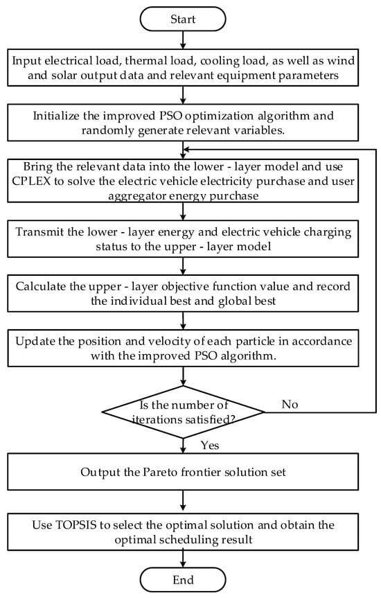
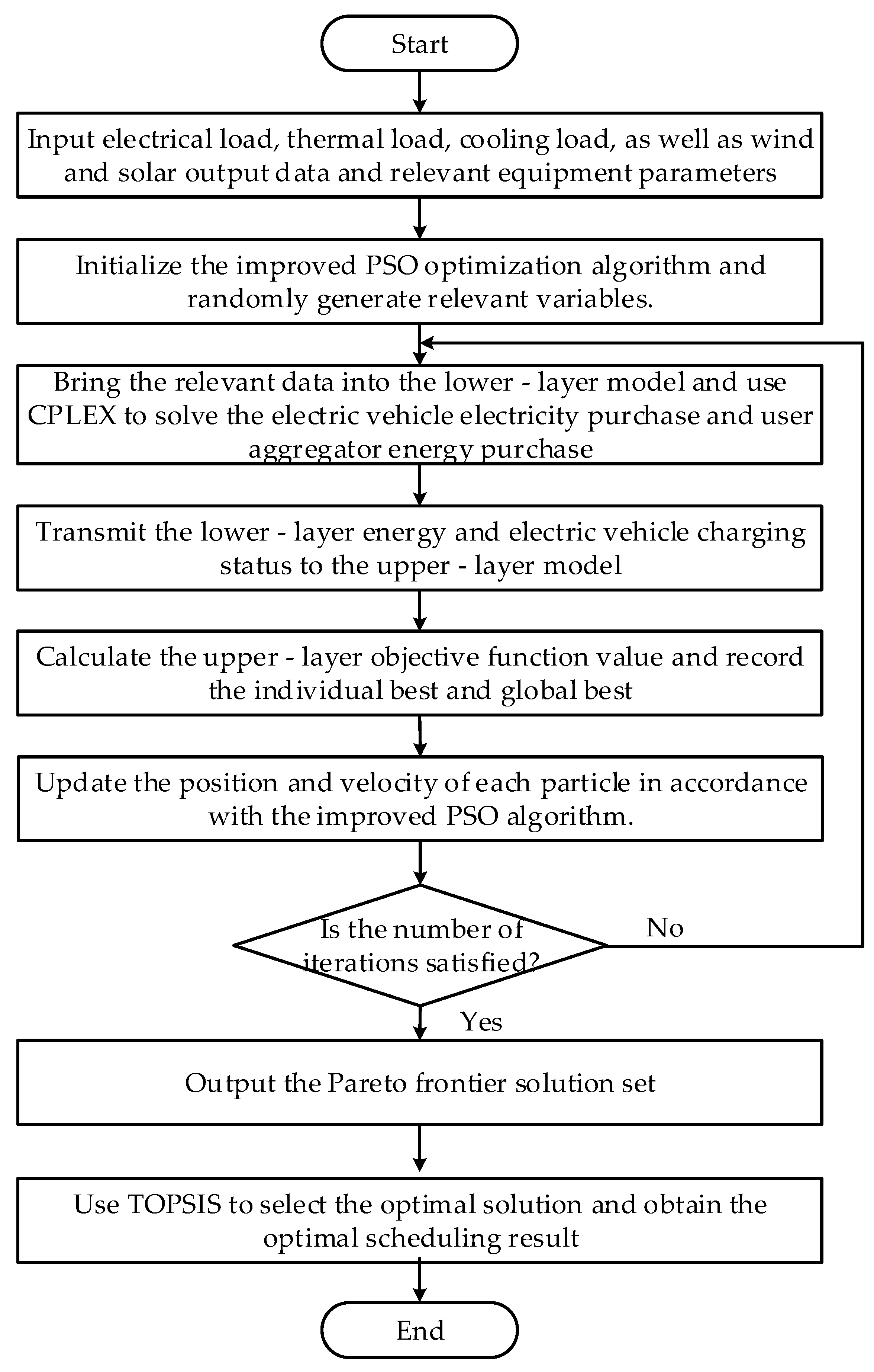
3.3.2. The Solution Procedure

The solution procedure of this paper is as follows:

• Input typical daily electric, thermal, and cooling load data, as well as wind and solar power output data, and relevant device parameters.
• Initialize the improved PSO algorithm, randomly generate relevant variables, and set the population size and maximum number of iterations.
• Solve the lower-level model using CPLEX 12.10 software to obtain the optimal values and transmit variables such as purchased energy to the upper-level model.
• Calculate the upper-level objective function values and record the individual best and global best solutions.
• Check if the maximum number of iterations is reached. If not, update the velocity and position of each particle according to the improved PSO algorithm, and transmit relevant energy price variables to the lower-level model. If yes, output the Pareto front solution set.
• Apply TOPSIS to select the optimal solution from the upper-level model and obtain the final dispatch results.

The solution process is shown in Figure 3.

Figure 3. Solution process of the bi-level optimization model.

4. Numerical Example and Result Analysis

4.1. Numerical Example Description

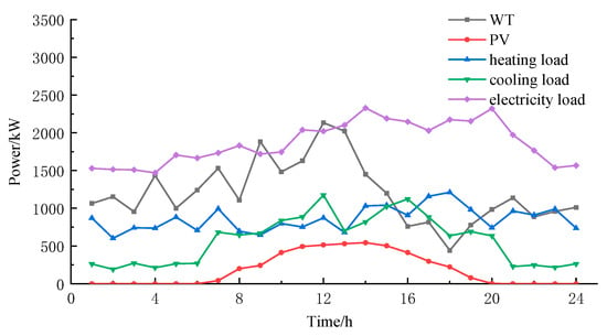
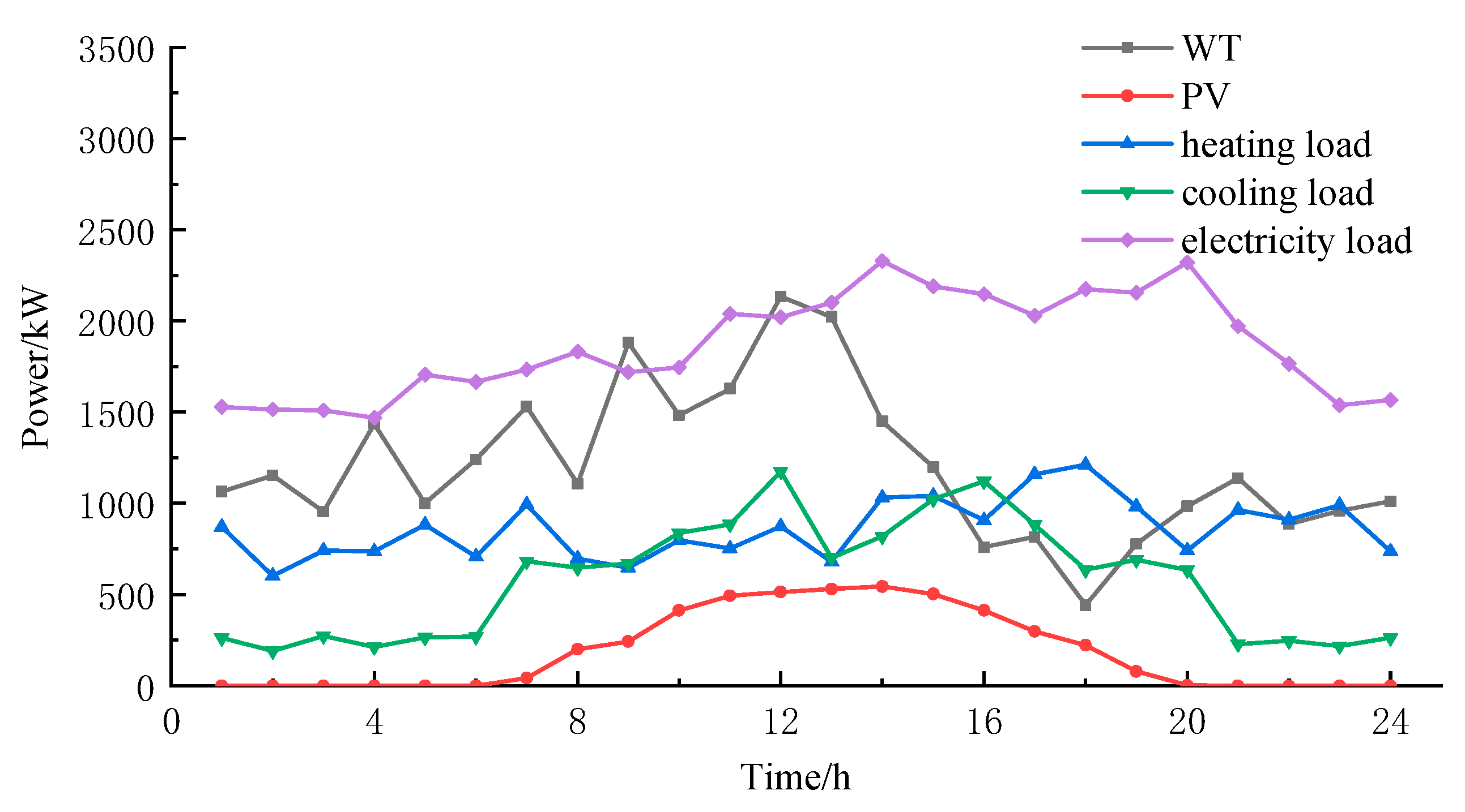
The Numerical example study selects a typical scenario in northern China. The predicted values of wind–solar combined power output, electricity, cooling, and heating loads are shown in Figure 4 [30]. The parameters of each device and energy storage in the IES are shown in Table 1 [30]. The demand response compensation prices are shown in Table 2. The interactive electricity prices between the IES and the large power grid are shown in Table 3 [31]. The parameters of electric vehicles are shown in Table 4 [30].

Figure 4. Output of renewable energy and load forecast curve.

Table 1. Parameters of various flexibility resources.

Equipment Name	Parameter	Value
Gas Turbine	Capacity (kW)	1000
	Electrical Efficiency	0.3
	Thermal Efficiency	0.45
	Ramping Constraint	25%
Electric Boiler	Capacity (kW)	500
	Thermal Efficiency	0.95
	Ramping Constraint	20%
Absorption Chiller	Capacity (kW)	1000
	Conversion Efficiency	0.7
	Ramping Constraint	20%
Electric Chiller	Capacity (kW)	500
	Conversion Efficiency	3.5
	Ramping Constraint	20%
Storage Battery	Capacity (kW)	500
	Capacity Upper/Lower Limit Constraint	0.95/0.1
	Ramping Constraint	25%
Heat Storage Tank	Capacity (kW)	500
	Capacity Upper/Lower Limit Constraint	0.95/0.1
	Ramping Constraint	25%

Table 2. Parameters related to demand response.

Load Type	Compensation Price/(yuan/kW·h)
Transferable Load	0.1
Curtailable Load	0.5
Substitutable Load	0.1

Table 3. Time-of-use electricity prices.

	Time Periods	Electricity Price/(yuan/kW·h)
Power Purchase	1:00–7:00, 23:00–24:00	0.4
	8:00–11:00, 15:00–18:00	0.75
	12:00–14:00, 19:00–22:00	1.2
Power Sale	1:00–7:00, 23:00–24:00	0.2
	8:00–11:00, 15:00–18:00	0.4
	12:00–14:00, 19:00–22:00	0.6

Table 4. Parameters of electric vehicles.

Category	Grid-Connection Time	Battery Capacity	Initial Electricity	Proportion
1	19:00–07:00	64	25	13%
2	9:00–17:00	40	25	20.2%
3	21:00–06:00	24	12	19.4%
4	10:00–17:00	32	16	26.4%
5	18:00–08:00	40	15	21%

The specific parameter settings are as follows: the population size was 50, and the maximum number of iterations was 200. A linearly decreasing inertia weight was adopted, decreasing from an initial value of 0.9 to 0.4 over the course of the iterations. The learning factors were set to $c_1=2$ and $c_2=1.5$. In multiple independent simulation runs, the algorithm consistently achieved stable convergence before reaching 200 iterations, thereby validating the effectiveness of the parameter configuration.

4.2. Scene Setting and Analysis of Scheduling Results

The effectiveness of the proposed flexibility-aware, multi-entity low-carbon economic scheduling model for IES was tested through five scenarios, as follows:

Scenario 1: Single economic objective at the upper level; multi-entity optimization with only aggregators at the lower level; no green certificate or carbon trading.

Scenario 2: Multi-objective optimization at the upper level; lower level unchanged from Scenario 1.

Scenario 3: Adds electric vehicles as participating entities to the lower-level optimization of Scenario 2.

Scenario 4: Introduces the carbon trading mechanism to Scenario 3.

Scenario 5: Further incorporates the green certificate mechanism, forming the complete green certificate carbon trading scheme within Scenario 4.

4.2.1. Analysis of IES Operator’s Operation Results

The scheduling results are shown in Table 5.

Table 5. Scheduling results of each Scenario.

	Scenario	1	2	3	4	5
IES Operator	Revenue	25,059	23,926	24,282	18,695	18,890
	Operating Cost	11,189	12,427	12,723	17,857	17,632
	Carbon Trading Cost	-	-	-	4867	4565
	Green Certificate Trading Cost	-	-	-		298
	Carbon Emissions	19,272	19,931	19,062	18,073	16,964
Electrical Energy Flexibility		0.25	0.30	0.35	0.36	0.36
Thermal Energy Flexibility		0.70	0.72	0.70	0.69	0.68
Cooling Energy Flexibility		0.73	0.83	0.82	0.76	0.77
System Flexibility		0.56	0.62	0.62	0.6	0.6
User Aggregator	Total Cost	39,735	39,795	39,799	39,801	39,809
	Energy Purchase Cost	36,248	36,292	36,297	35,986	35,949
	Demand Response Cost	3487	3503	3502	3815	3859
Electric Vehicles	Self-utility	-	-	6.24	6.26	6.27
	Charging Cost	-	-	569	566	573

As can be seen from Table 5, Scenario 2 conducts multi-objective optimization considering both economy and flexibility on the basis of Scenario 1. A balance between economic efficiency and system flexibility is achieved, with the IES operator incurring a revenue loss of 1133 yuan in exchange for a 10.7% enhancement in flexibility. The IES operator in Scenario 1 focused solely on economic goals, leading to a relaxation of flexibility demands in the pursuit of cost efficiency. Scenario 2, however, adopted a multi-objective approach that balanced economic and flexibility targets. Consequently, through targeted energy pricing policies, it effectively incentivized the demand-response resources and aggregated EV clusters to activate their regulatory capabilities. This coordinated response ultimately led to a quantifiable improvement in system flexibility. When electric vehicles are introduced as a flexibility resource in Scenario 2, the system incurs an additional 296 yuan in operating costs to meet their electricity demand. However, this investment yields a greater profit increase of 356 yuan. After electric vehicles are connected to the system as a flexibility resource, the system’s electrical energy flexibility is improved by 16.7%, indicating that electric vehicles play an important role in enhancing system flexibility as a flexibility resource.

Scenario 4 considers carbon trading costs based on Scenario 3, resulting in a decrease of 5587 yuan in the total profit of the IES operator and a reduction of 989 kg in carbon emissions. This reveals an inherent trade-off within the system, where the low-carbon objective and operational economic efficiency cannot be optimized simultaneously. Building upon Scenario 4, Scenario 5 introduces a green certificate trading mechanism. By offsetting a portion of carbon emissions through this mechanism, the system achieves an additional reduction of 1109 kg in carbon emissions. Consequently, carbon trading costs decrease by 302 yuan, while the system incurs an additional 298 yuan in green certificate trading costs. The introduction of carbon trading in Scenario 4 leads to a 5.19% reduction in system carbon emissions relative to Scenario 3. Subsequently, the incorporation of green certificate trading in Scenario 5 drives a further 6.19% decrease. The cross-scenario comparison of carbon emissions provides compelling evidence for the effectiveness of the green certificate carbon trading mechanism in mitigating emissions.

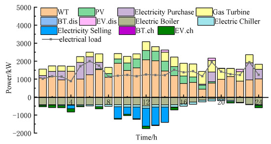
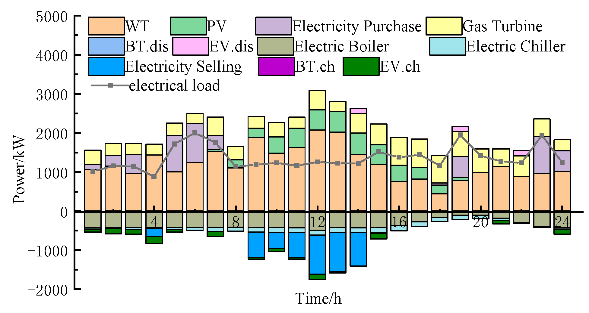
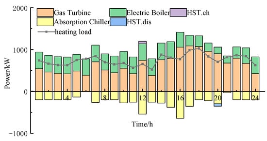
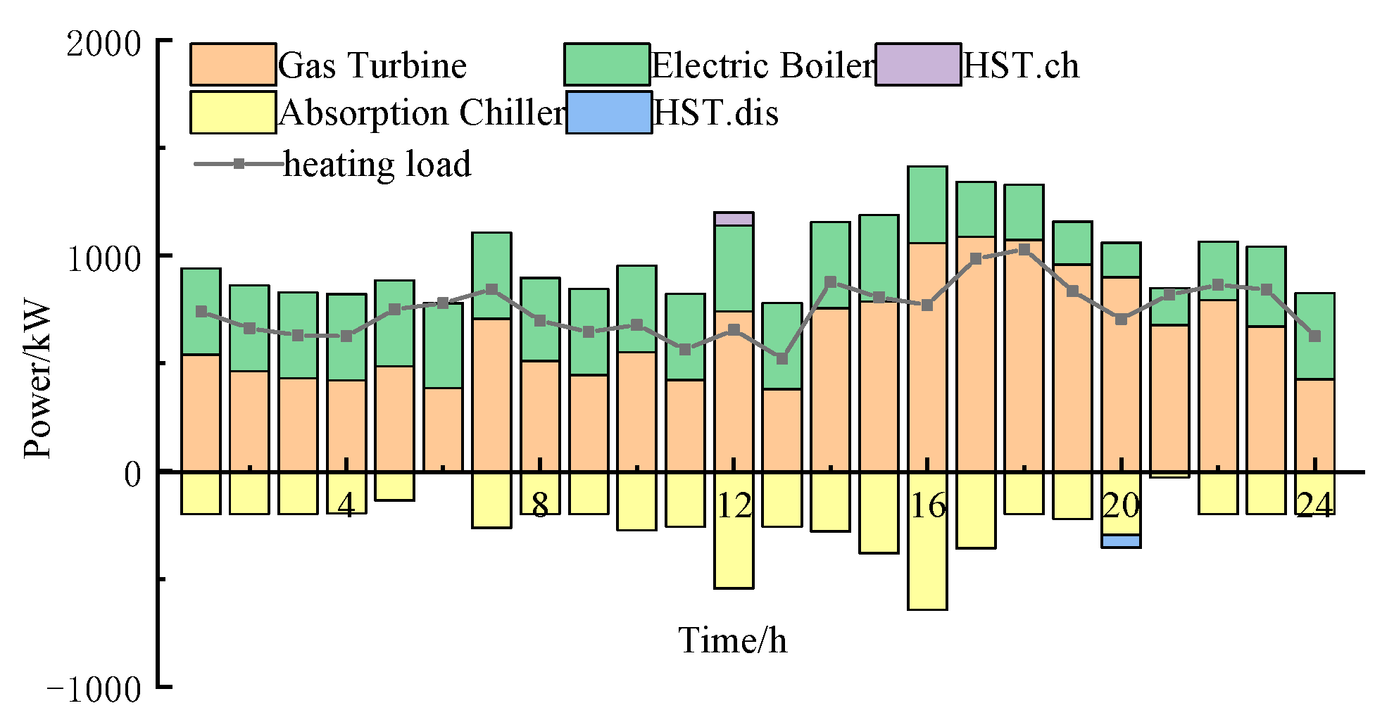
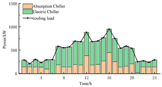
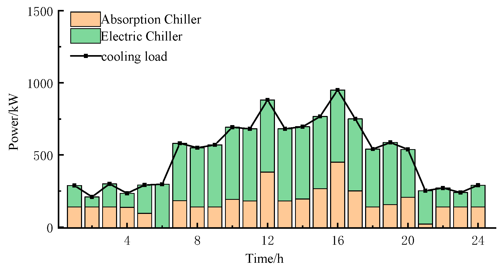
Figure 5, Figure 6, Figure 7 and Figure 8 show the optimization results of IES’s electricity, heat, and cooling power in Scenario 5. From the electricity power optimization results, it can be seen that the system tends to purchase electricity from the large power grid to reduce carbon emissions. Electric vehicles exert their energy storage characteristics, and on the premise of meeting their own charging needs, they replace batteries for charging and discharging to balance the system’s electricity power. From the heat power optimization, it can be observed that in the optimized operation considering the carbon trading mechanism, the system reduces the output of gas turbines and uses more electric boilers for power output; the heat storage tank releases heat at 12:00 when the heat supply is insufficient to meet the power balance. For cooling power, it is mainly provided by electric refrigerators, and the remaining cooling power is supplemented by absorption refrigerators.

Figure 5. Optimized electrical power results in Scenario 5.

Figure 6. Optimized heating power results in Scenario 5.

Figure 7. Optimized cooling power results in Scenario 5.

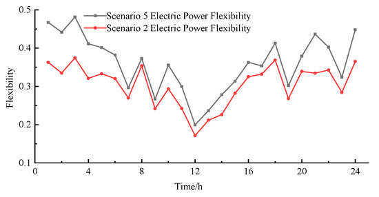
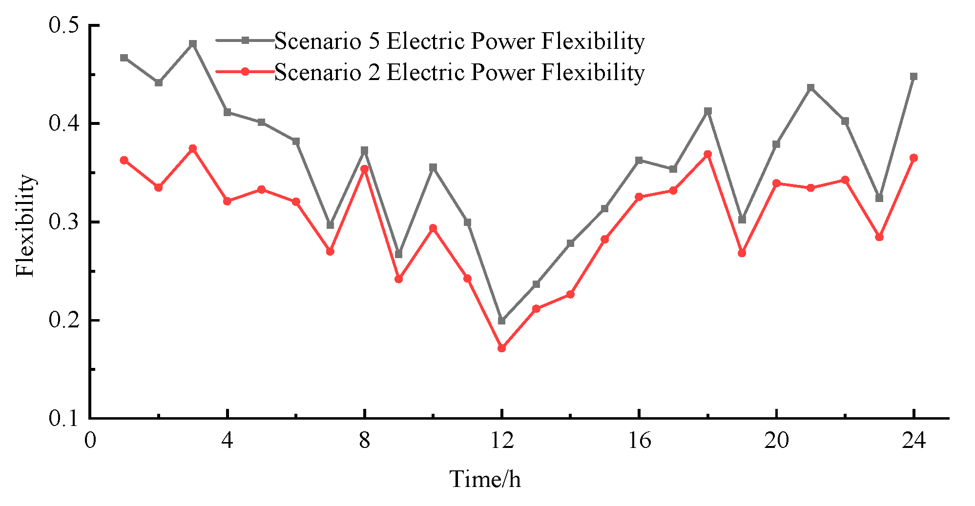
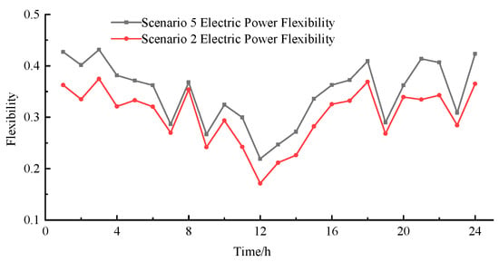
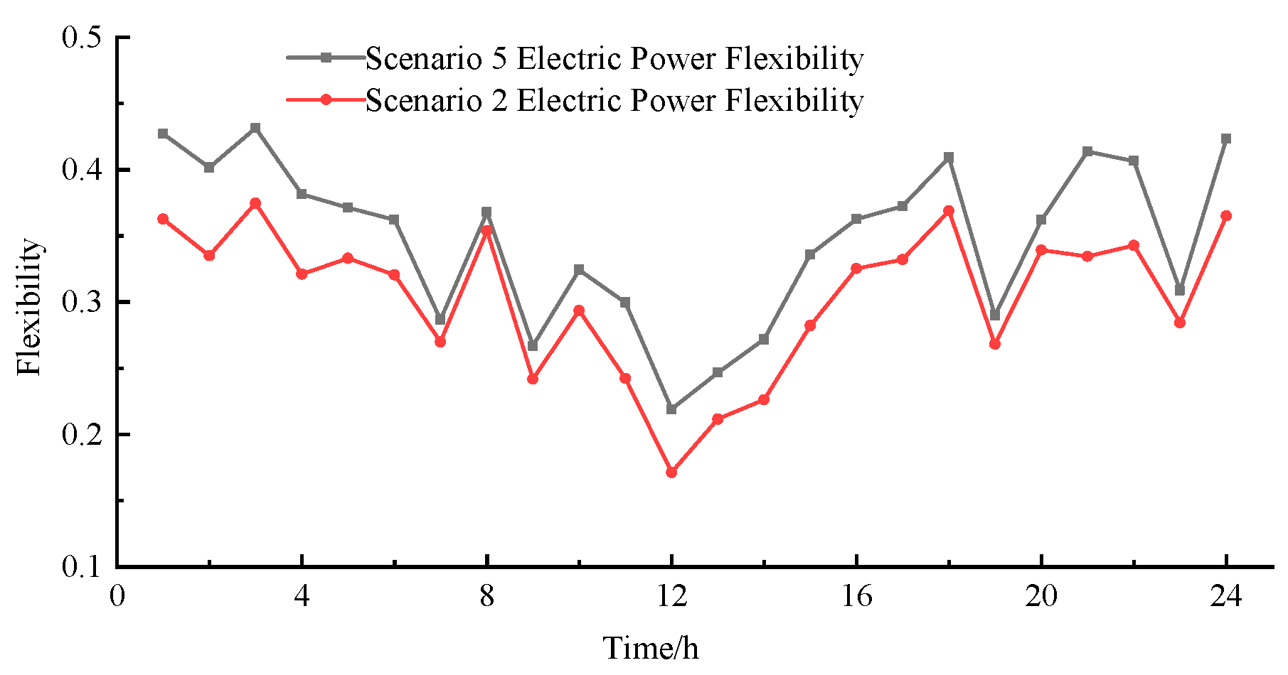
Figure 8. Electrical energy flexibility in Scenario 5 and Scenario 2.

Figure 8 shows the comparison results of system flexibility between Scenario 5 and Scenario 2. The flexibility provided by electric vehicles to the system is affected by their grid-connection time. Since most electric vehicles are in the grid-connection state from 18:00 to 8:00, it can be seen from the figure that the system flexibility is significantly improved during this period.

4.2.2. Analysis of User Aggregator’s Operation Results

As a primary participant in the IES optimal scheduling, the user aggregator’s cost performance across the five scenarios can be observed in Table 5. The highest total cost is 39,809 yuan, while the lowest is 39,735 yuan, resulting in a narrow range of only 74 yuan. This demonstrates that the user aggregator is able to keep its overall costs relatively stable by leveraging the demand response mechanism to adapt to variations in system resources. For instance, when comparing Scenario 3 with Scenario 5—where the IES operator faces reduced revenue due to the inclusion of green certificate-carbon trading costs—the user aggregator raises its demand response expenditure by 357 yuan to counteract the operational cost increase driven by energy price fluctuations, thereby preserving cost stability.

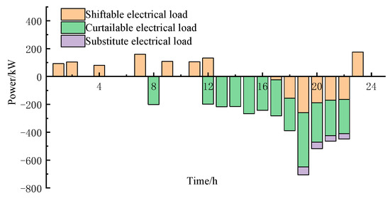
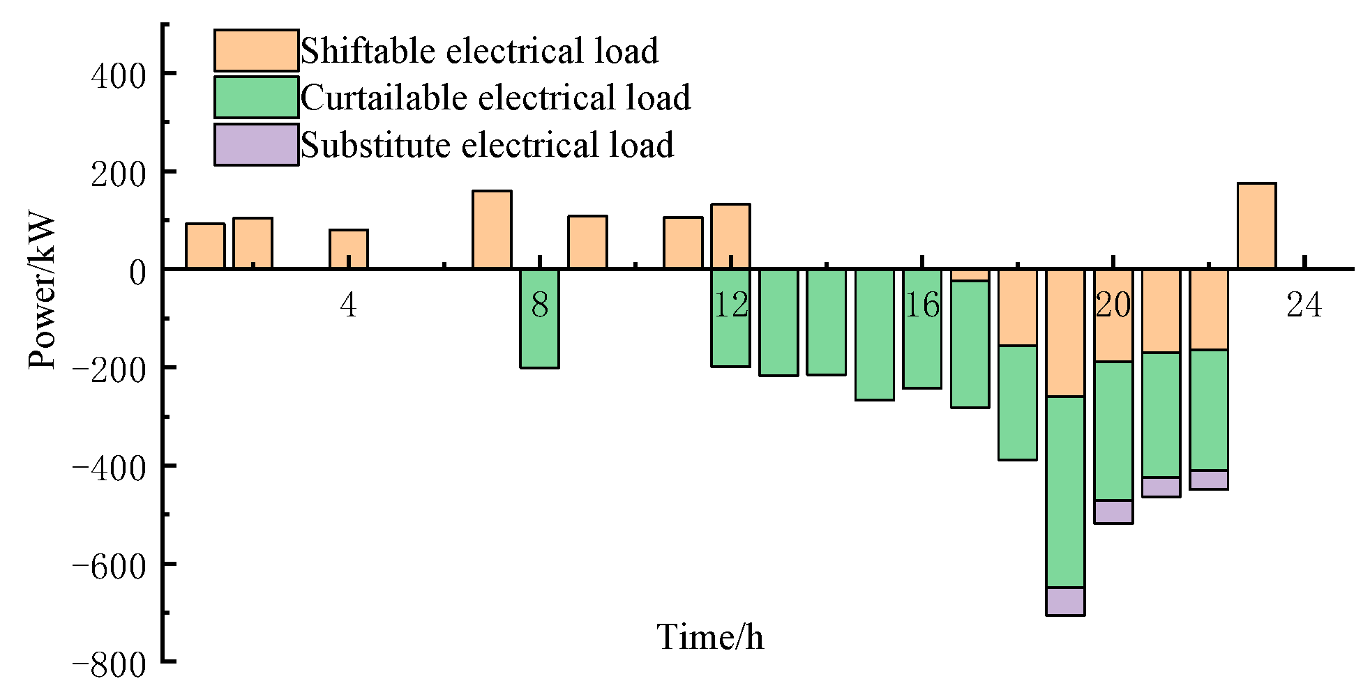
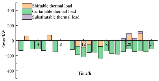
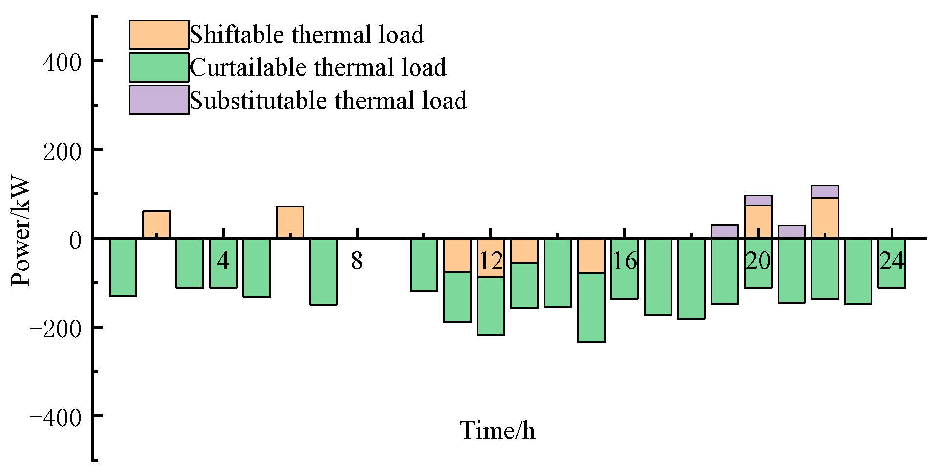
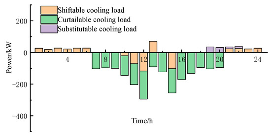
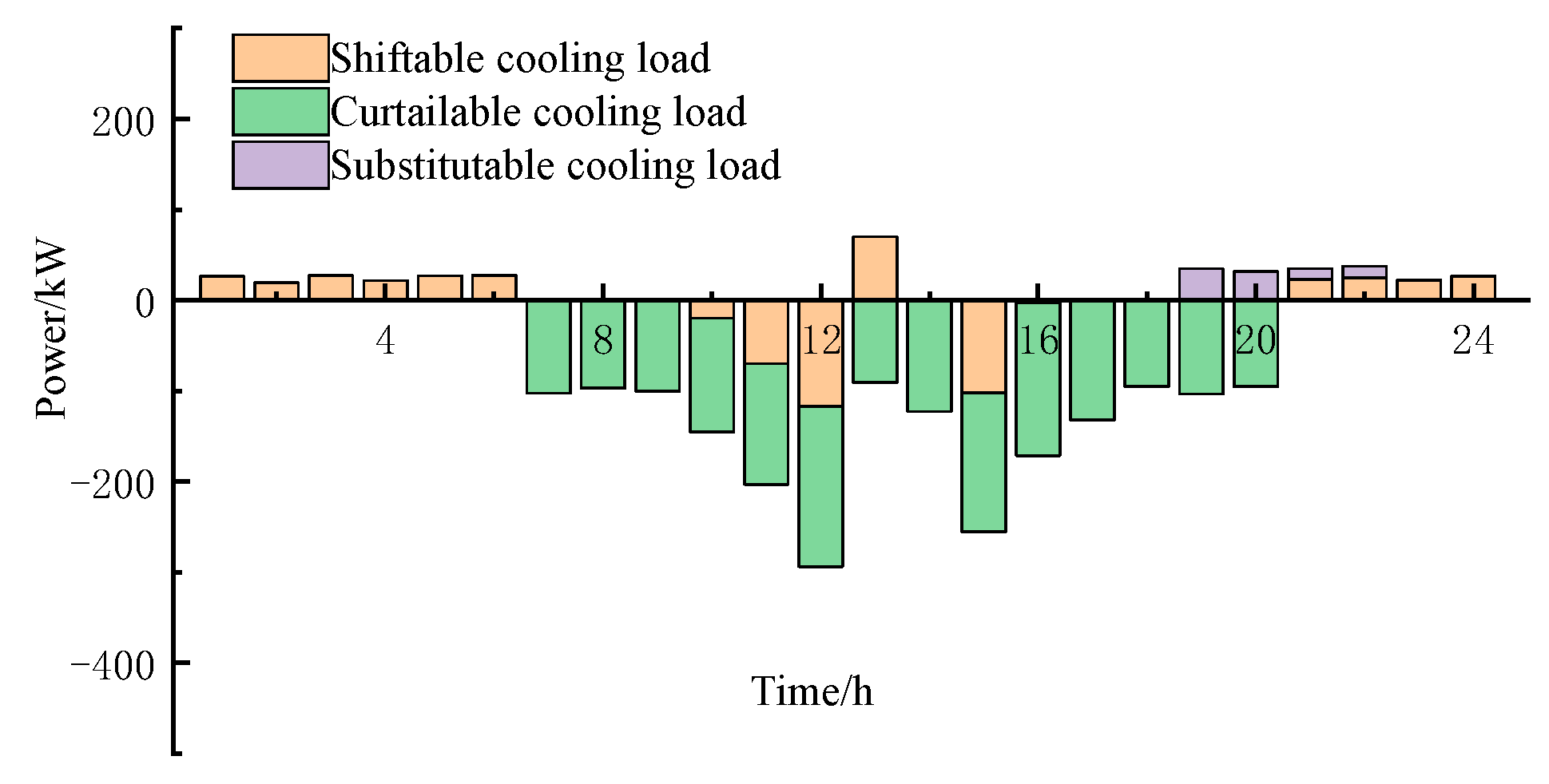
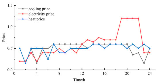
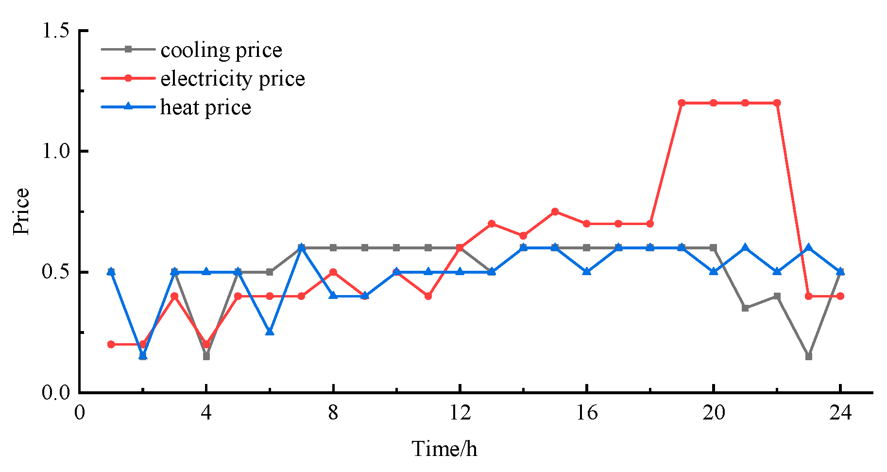
Figure 9, Figure 10, Figure 11 and Figure 12 show the demand response results and energy purchase prices of the user aggregator. The optimization results indicate that the maximum prices of cooling energy, electricity, and thermal energy are 0.6 yuan, 1.2 yuan, and 0.6 yuan respectively, and the minimum prices are 0.15 yuan, 0.2 yuan, and 0.15 yuan. When there are significant differences between the electricity price and the thermal/cooling prices, such as from 19:00 to 22:00, energy substitution is carried out to reduce energy purchase costs.

Figure 9. Electricity demand response results in Scenario 5.

Figure 10. Thermal power demand response results in Scenario 5.

Figure 11. Cooling power demand response results in Scenario 5.

Figure 12. Power price in Scenario 5.

4.2.3. Analysis of Electric Vehicle Operation Results

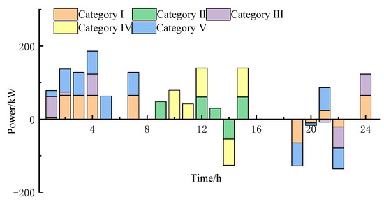
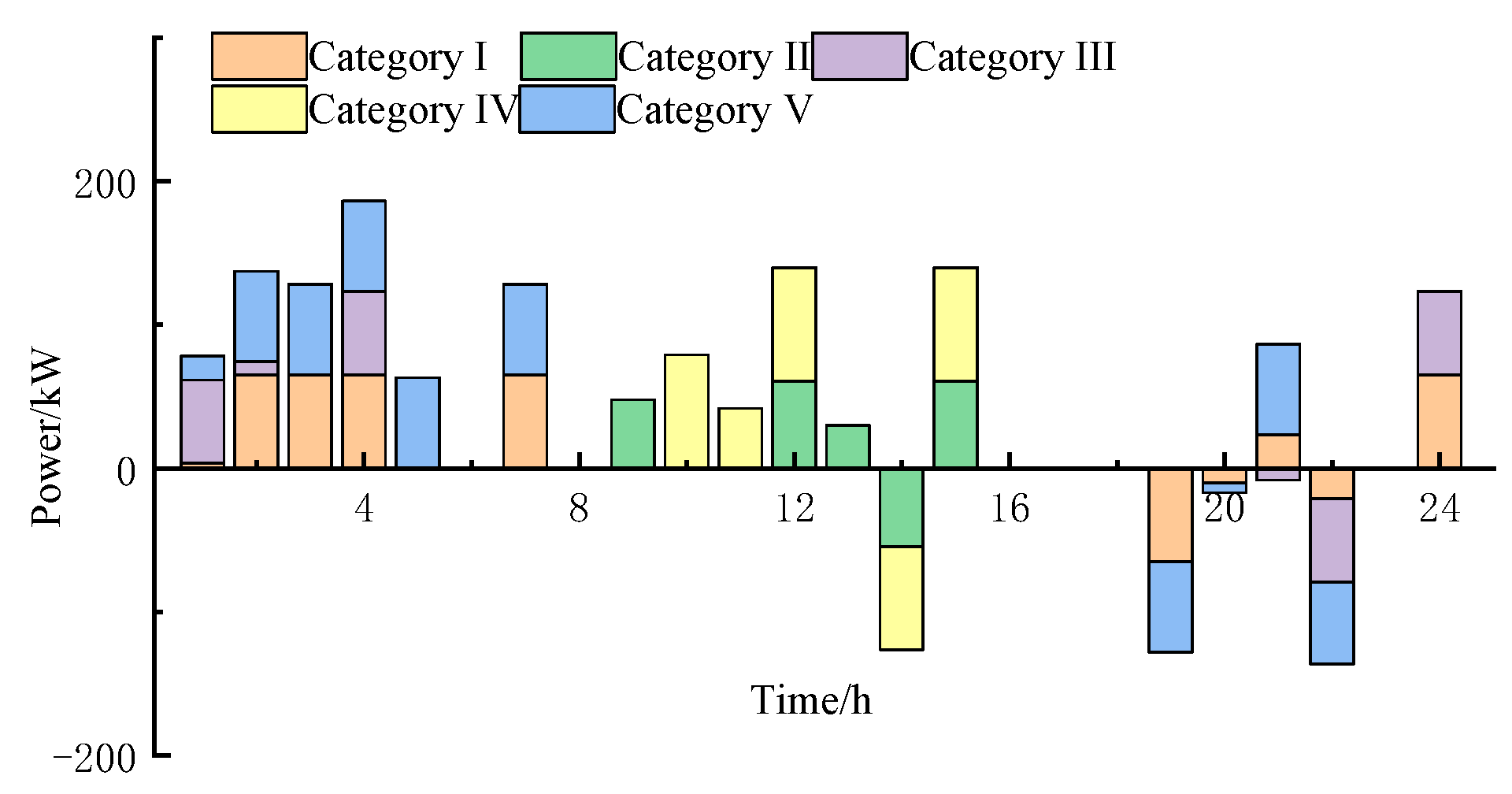
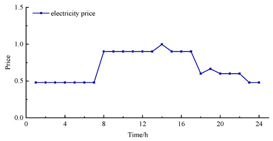
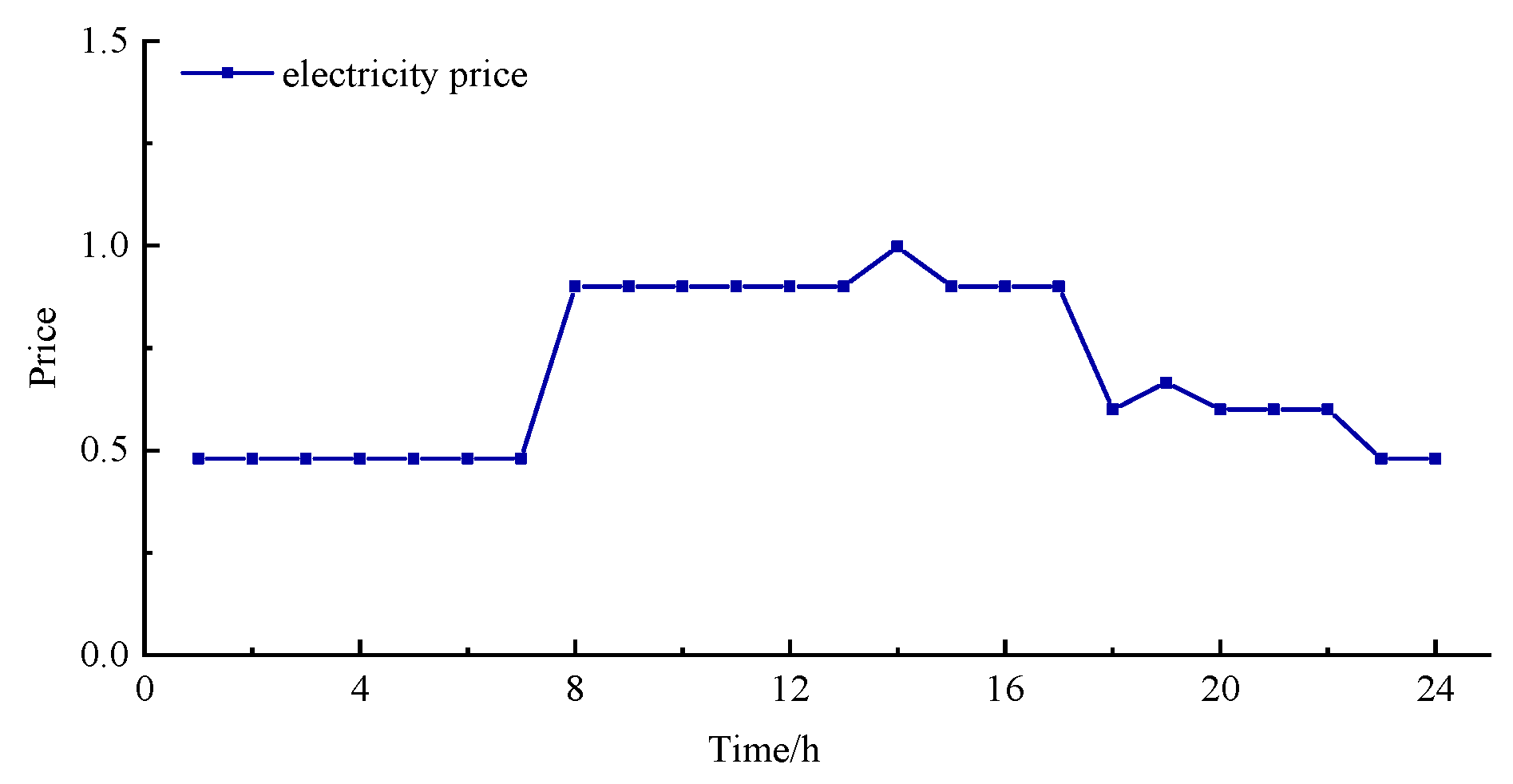
As indicated in Table 5, in scenarios where electric vehicles participate, both their own utility functions and charging costs can retain stable levels. The charging and discharging powers and prices of the five categories of electric vehicles in Scenario 5 are shown in Figure 13 and Figure 14. It can be seen from Figure 14 that the charging and discharging prices of electric vehicles fluctuate between 0.48 and 1 yuan/kWh, providing a flexible space for electric vehicles to choose charging and discharging. Electric vehicles choose appropriate times to charge and discharge to maximize their own utility functions. Taking the first category of electric vehicles as an example, they do not choose to charge immediately after being connected to the grid, but instead choose to discharge during periods with relatively high prices. Upon reaching 21:00, they initiate charging but discharge again at 22:00. Subsequently, they recharge prior to disconnection to ensure a fully charged state when leaving the grid, thus satisfying travel demands.

Figure 13. Electric vehicle charging and discharging power.

Figure 14. Electric vehicle charging and discharging prices.

4.2.4. Parameter Sensitivity Analysis

To investigate the impact of different carbon trading prices on scheduling results, while keeping other parameters unchanged, the carbon trading base price is increased to 1.05 times and 1.1 times the original value, respectively. The system carbon emissions and IES operator revenue results are shown in Table 6.

Table 6. Scheduling results under different carbon trading base prices.

Carbon Price Multiples Relative to the Base Price	1.0	1.05	1.1
Carbon Emissions/(t)	16,964	16,645	16,372
Revenue of IES operator/(yuan)	18,890	18,552	18,215

Adjustments to the carbon trading base price reveal that as the price increases, the system preferentially adopts low-carbon scheduling strategies. This shift leads to a continuous decline in overall carbon emissions, thereby enhancing carbon reduction effectiveness. This is accompanied by a rise in carbon trading costs, which directly increases the system’s operational expenses and consequently reduces its revenue. This dynamic clearly illustrates the classic trade-off between carbon reduction benefits and economic profitability.

As can be seen from Figure 8, the power flexibility of electric vehicles has significantly improved after participating in system optimization scheduling, but the flexibility at 12:00 is 0.2, which is still relatively low. To enhance the power flexibility at this specific time, the access ratios of various types of electric vehicles in Table 4 are adjusted to 13%, 30.2%, 9.4%, 36.4%, and 11%, respectively. The resulting flexibility outcomes are presented in Figure 15.

Figure 15. Electrical energy flexibility in Scenario 5 and Scenario 2 (under the new ratio of EV type).

As observed in Figure 15, the power flexibility index of the IES in Scenario 5 demonstrates a notable rise from 0.2 to 0.22 at 12:00, reflecting a 10% improvement and a marked enhancement in flexibility performance. Such improvement can be primarily explained by the strategic involvement of electric vehicles in coordinated charging and discharging within the dispatch framework, which reinforces the system’s capability to counteract power fluctuations and strengthens its reserve capacity. These results highlight the essential function of electric vehicles as flexible and dispatchable resources in broadening the power regulation scope of IES.

4.3. Analysis of the Effect of the Improved Particle Swarm Optimization Algorithm

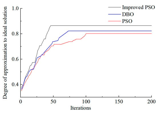
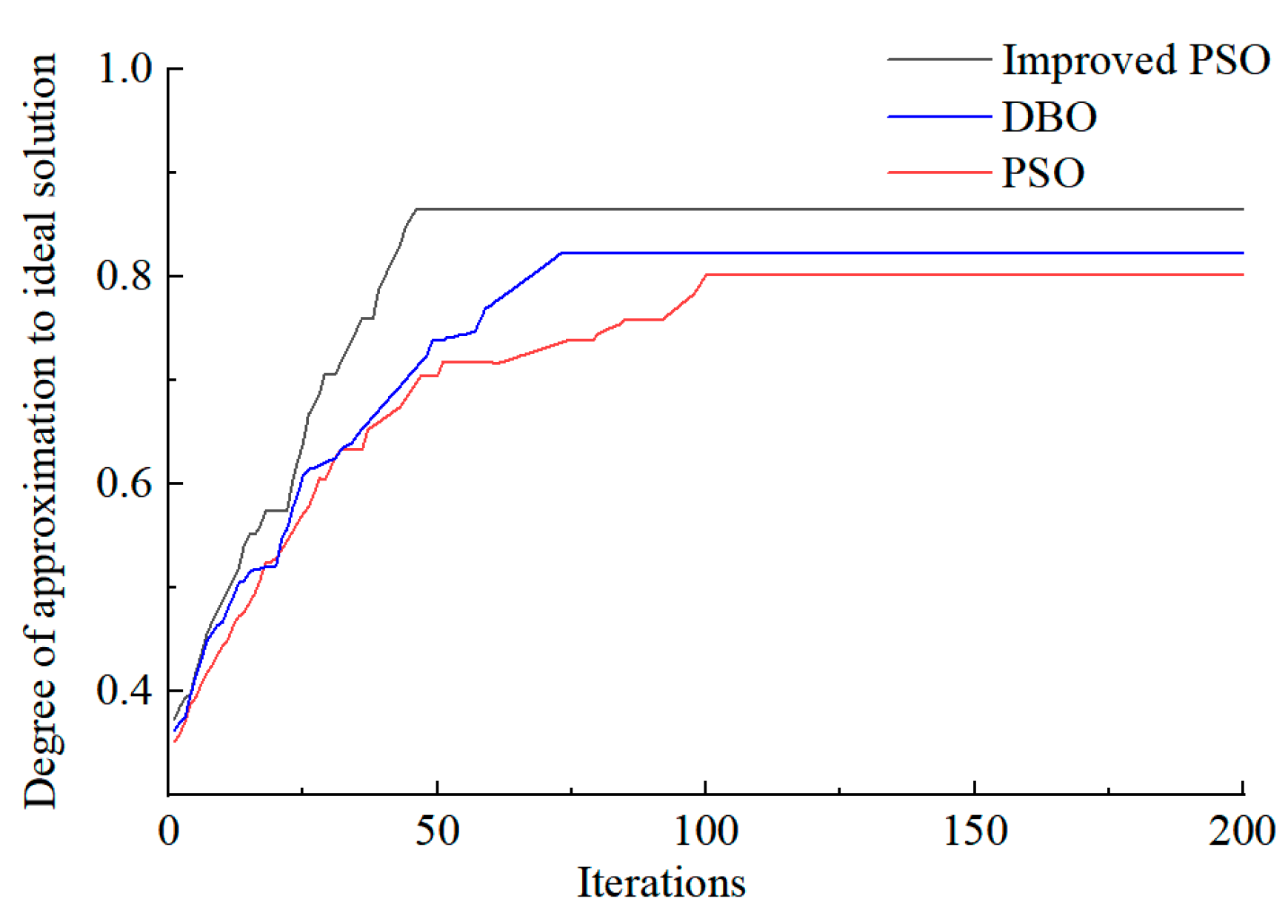
To verify the effectiveness of the improved strategy proposed in this paper, the PSO algorithm, DBO algorithm and the improved PSO algorithm are adopted in solving the upper-layer model of Scenario 5, with the number of iterations set to 200. The Technique for Order Preference by Similarity to Ideal Solution (TOPSIS) is used to calculate the relative proximity between the Pareto optimal solution and the ideal solution for evaluating the optimization results, and the convergence situation is shown in Figure 16.

Figure 16. Comparison of algorithm iterations.

It can be seen from Figure 15 that when the PSO algorithm is adopted, convergence is achieved after 100 iterations, with the proximity to the ideal solution being 0.80; when the DBO algorithm is adopted, convergence is achieved after 73 iterations, with the proximity to the ideal solution being 0.82; when the improved PSO algorithm proposed in this paper is adopted, convergence is achieved after 46 iterations, with the proximity being 0.86. Through comparison, it can be concluded that the improved PSO algorithm adopted in this paper has better convergence and optimization performance compared with the PSO and DBO algorithms. Compared to PSO, the improved PSO algorithm reduced the number of iterations at convergence by 54.0%, improved the closeness of the obtained optimal solution to the ideal solution by 7.5%, and had better convergence and optimization performance.

To evaluate algorithm stability, we further examined the results of multiple independent runs for each algorithm with the population size set to 50 and the number of iterations to 200; each algorithm was independently run 30 times, as presented in Table 7. These results include statistics on the convergence of the obtained results toward the ideal solution along with the runtime.

Table 7. Results of multiple independent runs of various algorithms.

Algorithm	Maximum	Mean	Variance	Runtime/(s)
PSO	0.8	0.786	7.892 × 10−5	134
DBO	0.82	0.808	6.485 × 10−5	117
IPSO	0.86	0.849	5.733 × 10−5	105

As indicated in Table 7, the improved Particle Swarm Optimization (IPSO) exhibits the most favorable comprehensive performance in terms of maximum value, average value, variance, and runtime. Regarding optimization efficacy, IPSO attains a maximum value of 0.86 and an average value of 0.849, both surpassing those achieved by the conventional Particle Swarm Optimization (PSO) and the Dung Beetle Optimizer (DBO). The fact that IPSO consistently yields higher objective function values substantiates its enhanced global search capability and superior optimization precision. In terms of stability, the variance of IPSO is 5.733 × 10⁻⁵, which is lower than that of PSO and DBO. This indicates that the results of the algorithm are more concentrated and have smaller fluctuations across multiple runs, demonstrating higher robustness and solution stability.

5. Conclusions

Focusing on system flexibility, this paper investigates the diverse flexibility resources in IES and develops a corresponding multi-objective optimization model for low-carbon economic dispatch that integrates flexibility requirements and multi-entity participation. The study yields the following conclusions.

(1)

In the case study of this paper, the proposed multi-entity optimal dispatch model successfully balanced the interests among the specific stakeholders modeled, namely the IES operator, user aggregators, and EV clusters. Simulation results demonstrated that under this framework, IES operators can make trade-off choices in scheduling plans between economy and flexibility. Guided by energy prices, the user aggregator manages demand response to achieve cost stability despite resource variability within the system. Furthermore, the integrated EV clusters, managed as flexible resources within the model, their scheduled charging/discharging actions directly enhanced the system’s operational flexibility.

(2)

The proposed mechanism considering the carbon trading and the green certificate trading mechanism can reduce system carbon emissions. The introduction of carbon trading in Scenario 4 leads to a 5.19% reduction in system carbon emissions relative to Scenario 3. Subsequently, the incorporation of green certificate trading in Scenario 5 drives a further 6.19% decrease.

(3)

Compared to PSO, the improved PSO algorithm in this work reduced the number of iterations at convergence by 54.0%, improved the closeness of the obtained optimal solution to the ideal solution by 7.5%, and has better convergence and optimization performance.

The research focus of this paper is the park-level IES, which has a certain reference value for regional-level IES and will also serve as the direction for future work. Future studies should include updated, realistic electricity costs and device parameters to empirically verify the results presented in this paper. Furthermore, flexibility indicators and the aggregation characteristics of electric vehicles can also be expressed using probabilistic indicators to address system randomness.

References

- Zhong, H.; Zhang, N.; Du, E.; Guo, H.; Cai, Y.; Wang, P.; Gao, H.; Li, Y.; Liu, X.; Kang, C. Planning, operation and market of new power system: Research progress and practice. Proc. CSEE 2024, 44, 7084–7104. [Google Scholar]
- Huang, W.; Zhang, N.; Cheng, Y.; Yang, J.; Wang, Y.; Kang, C. Multi energy networks analytics: Standardized modeling, optimization, and low carbon analysis. Proc. IEEE 2020, 108, 1411–1436. [Google Scholar] [CrossRef] [Scilit]
- Zhou, J.; Liang, C.; Shi, L.; Li, Y.; Yi, W. Optimized dispatch of integrated energy systems considering a tiered carbon trading mechanism. China Electr. Power 2025, 58, 77–87. [Google Scholar] [CrossRef]
- Fan, X.; Chen, K.; Chen, Y. Is price commitment a better solution to control carbon emissions and promote technology investment? Manag. Sci. 2023, 69, 325–341. [Google Scholar] [CrossRef] [Scilit]
- Chen, H.; Ma, G.; Qian, D.; Ma, J.; Peng, Y. Optimized dispatch of regional integrated energy systems considering tiered demand response under green certificate-carbon trading mechanism. Integr. Smart Energy 2025, 47, 21–30. [Google Scholar] [CrossRef]
- Li, H.; Wu, J.; Wang, J.; Zhang, Y.; Liu, Y. Low-carbon economic dispatch of a wind, solar, and hydrogen storage integrated energy system considering P2G and carbon capture. Power Syst. Prot. Control 2024, 52, 26–36. [Google Scholar]
- Yang, M.; Wang, Y.; Wang, J.; Liu, D.; Xu, W. Optimal scheduling of integrated energy systems in low-carbon communities considering flexibility of resources and segmental control of solid oxide fuel cells. J. Mod. Power Syst. Clean Energy 2025, 13, 915–927. [Google Scholar] [CrossRef] [Scilit]
- Mahmud, S.; Ponkiya, B.; Katikaneni, S.; Pandey, S.; Mattimadugu, K.; Yi, Z.; Walker, V.; Wang, C.; Westover, T.; Javaid, A.; et al. Design and optimization of a modular hydrogen-based integrated energy system to maximize revenue via nuclear-renewable sources. Energy 2024, 313, 133763. [Google Scholar] [CrossRef] [Scilit]
- Yuan, T.; Zhang, W. A review of research on coordinated planning of source-storage-load in new power systems. Proc. CSEE. 2024, 45, 6664–6682. [Google Scholar] [CrossRef]
- Chicco, G.; Riaz, S.; Mazza, A.; Mancarella, P. Flexibility from distributed multienergy systems. Proc. IEEE 2020, 108, 1496–1517. [Google Scholar] [CrossRef] [Scilit]
- Mohandes, B.; Moursi, M.; Hatziargyriou, N.; Khatib, S. A review of power system flexibility with high penetration of renewables. IEEE Trans. Power Syst. 2019, 34, 3140–3155. [Google Scholar] [CrossRef] [Scilit]
- De, G.; Wang, X.; Tian, X.; Xu, T.; Tan, Z. A collaborative optimization model for integrated energy system considering multi-load demand response. Energies 2022, 15, 2033. [Google Scholar] [CrossRef] [Scilit]
- Zhou, J.; Li, S.; Meng, T.; Liu, S.; Liang, G. Multi-objective optimization of integrated energy systems based on demand response. Energy Sources Part A Recovery Util. Environ. Eff. 2023, 45, 1204–1225. [Google Scholar]
- Pan, C.; Fan, G.; Wang, J.; Xu, X.; Meng, T. Low-carbon optimization of electric-heat integrated energy systems with the participation of flexible resources. Trans. China Electrotech. Soc. 2023, 38, 1633–1647. [Google Scholar]
- Shen, J.; Wang, Y.; Cheng, C.; Zhang, C.; Zhou, B. Quantification of flexibility demand and coordinated optimization model for water-wind-solar complementary systems. J. Hydraul. Eng. 2022, 53, 1291–1303. [Google Scholar]
- Zhang, X.; Wang, Q.; Yu, J.; Sun, Q.; Hu, H.; Liu, X. A multi-agent deep-reinforcement-learning-based strategy for safe distributed energy resource scheduling in energy hubs. Electronics 2023, 12, 4763. [Google Scholar] [CrossRef] [Scilit]
- Nie, L.; Long, B.; Yu, M.; Zhang, D.; Yang, X.; Jing, S. A low-carbon economic scheduling strategy for multi-microgrids with communication mechanism-enabled multi-agent deep reinforcement learning. Electronics 2025, 14, 2251. [Google Scholar] [CrossRef] [Scilit]
- Arvanitidis, A.I.; Alamaniotis, M. Optimal Security Constrained Economic Dispatch in Nuclear Integrated Energy Systems. In Proceedings of the 2025 IEEE Texas Power and Energy Conference (TPEC), College Station, TX, USA, 10–11 February 2025; pp. 1–6. [Google Scholar]
- Zhang, L.; Sun, C.; Cai, G.; Koh, L. Charging and discharging optimization strategy for electric vehicles considering elasticity demand response. ETransportation 2023, 18, 100262. [Google Scholar] [CrossRef] [Scilit]
- Jahic, A.; Heider, F.; Plenz, M.; Schulz, D. Flexibility quantification and the potential for its usage in the case of electric bus depots with unidirectional charging. Energies 2022, 15, 3639. [Google Scholar] [CrossRef] [Scilit]
- Ma, Y.; Guo, X.; Chen, R.; Xie, X.; Wang, R.; Shen, D.; Wang, F.; Zhou, D. Coordinated planning of electricity-gas integrated energy systems based on multi-agent benefits. Smart Power 2021, 49, 1–6. [Google Scholar]
- Li, Y.; Wang, C.; Li, G.; Chen, C. Optimal scheduling of integrated demand response-enabled integrated energy systems with uncertain renewable generations: A Stackelberg game approach. Energy Convers. Manag. 2021, 235, 113996. [Google Scholar] [CrossRef] [Scilit]
- Yang, J.; Xu, W.; Ma, K.; Chen, J.; Guo, W. Integrated demand-side management for multi-energy system based on non-cooperative game and multi-energy pricing. Sustain. Energy Grids Netw. 2023, 34, 101047. [Google Scholar] [CrossRef] [Scilit]
- Wang, Y.; Dou, W.; Tong, Y.; Yang, B.; Zhu, H.; Xu, R.; Yan, N. Optimal configuration method of electric vehicle’s participating in Load Aggregator’s VPP low-carbon economy. Energy Rep. 2023, 9, 1093–1100. [Google Scholar] [CrossRef] [Scilit]
- Zheng, J.; Zhai, L.; Li, F.; Wang, D.; Li, Y.; Li, Z.; Wu, Q. Multi-objective optimization and multi-attribute decision-making support for optimal operation of multi stakeholder integrated energy systems. Appl. Soft Comput. 2024, 167, 112426. [Google Scholar] [CrossRef] [Scilit]
- Zhang, Y.; Li, J.; Ji, X.; Wu, H.; Li, S.; Wen, F. Bi-level Game Dispatch of Park Integrated Energy System Considering Decision-making Synergy of Electricity-Carbon Markets. Autom. Electr. Power Syst. 2025, 49, 45–59. [Google Scholar]
- Liu, Y.; Xin, M.; Qin, H.; Shan, H. Hybrid Game-based Optimal Scheduling of Energy System Operator and Regional Integrated Energy System Alliance Considering Risk of Carbon Emission Right Trading. Electr. Power Autom. Equip. 2025, 45, 15–22. [Google Scholar]
- Liu, X.; Xie, S.; Tian, J.; Wang, P. Two-stage scheduling strategy for integrated energy systems considering renewable energy consumption. IEEE Access 2022, 10, 83336–83349. [Google Scholar] [CrossRef] [Scilit]
- Xie, J. Low-Carbon Economic Dispatch of Park Integrated Energy System Considering the Green Certificate-Carbon Joint Trading Mechanism. Master’s Thesis, Yanshan University, Qinhuangdao, China, 2025. [Google Scholar]
- Du, H. Research on Collaborative Optimization Configuration of Integrated Energy Systems Considering Electricity Heating Cooling Demand Response. Master’s Thesis, Northeast Electric Power University, Jilin, China, 2025. [Google Scholar]
- Lu, J.; Liang, N.; Xu, H.; Xu, Y.; Tian, Y.; Shang, Y. Coordinated optimal dispatch of multiple Integrated energy systems under dynamic car-bon-green certificate trading interaction mechanism. Autom. Electr. Power Syst. 2025, 49, 52–60. [Google Scholar] [CrossRef]
Disclaimer/Publisher’s Note: The statements, opinions and data contained in all publications are solely those of the individual author(s) and contributor(s) and not of MDPI and/or the editor(s). MDPI and/or the editor(s) disclaim responsibility for any injury to people or property resulting from any ideas, methods, instructions or products referred to in the content. |
© 2026 by the authors. Licensee MDPI, Basel, Switzerland. This article is an open access article distributed under the terms and conditions of the Creative Commons Attribution (CC BY) license.