Tunnel-SLAM: Low-Cost LiDAR/Vision/RTK/Inertial Integration on Vehicles for Roadway Tunnels

Abstract

Reliable positioning and mapping in roadway tunnels are crucial for vehicle-based monitoring and inspection, especially considering the challenging environmental conditions such as rapidly changing illumination, low-texture environments, and repetitive structural elements. While general LiDAR-inertial odometry (LIO) frameworks and loop-closure detection methods are effective in general scenarios, they often suffer from severe drift or incorrect loop constraints under these specific conditions. These challenges are further exacerbated by the inherent uncertainties associated with low-cost sensors. This paper introduces a narrow field-of-view LiDAR-centric RTK-visual-inertial SLAM system enhanced by three key modules: semantic-assisted loop detection and matching, two-stage RTK quality control, and adaptive factor graph optimization (FGO). In the first module, the proposed semantic loop descriptor (SLD) matching is used to determine the potential loop closure locations and then integrates the corresponding constraint as graph nodes. The quality control module addresses RTK outlier rejection during tunnel entry and exit, employing an event-driven stochastic model to characterize the uncertainty between RTK and the other sensors, effectively suppressing RTK-induced errors. FGO module performs optimization by incorporating LIO, RTK, and loop closure factors, employing a keyframe-based strategy to produce globally optimized poses while continuously updating the map. The proposed Tunnel-SLAM was evaluated against state-of-the-art SLAM algorithms in four extended roadway tunnels, ranging in traveling distance approximately from 5 to 10 km. Experimental results demonstrate that the proposed SLAM achieved a final drift of less than 2 m with loop closure, demonstrating significantly reducing the drift, while other existing SLAM frameworks fail catastrophically or have large drift.

1. Introduction

Pose estimation and map construction of the surrounding environment are fundamental components for roadway tunnel inspection and monitoring [1]. Traditional methods often rely on RTKs (real-time kinematics) or GNSSs (global navigation satellite system) integrated with inertial sensors to provide pose information and geodetic coordinate references. However, in GNSS-denied roadway tunnels, the reliance shifts to high-precision but costly inertial sensors such as fiber-optic gyroscopes to ensure continuous trajectory tracking. This is because consumer-grade GNSS/INSs are highly susceptible to significant drift over time. Even with advanced inertial navigation systems (INSs), drift remains a persistent challenge in long tunnels environments, posing a critical barrier to the widespread deployment of intelligent tunnel inspection technologies and potentially increasing risks in tunnel management.

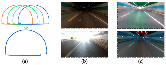
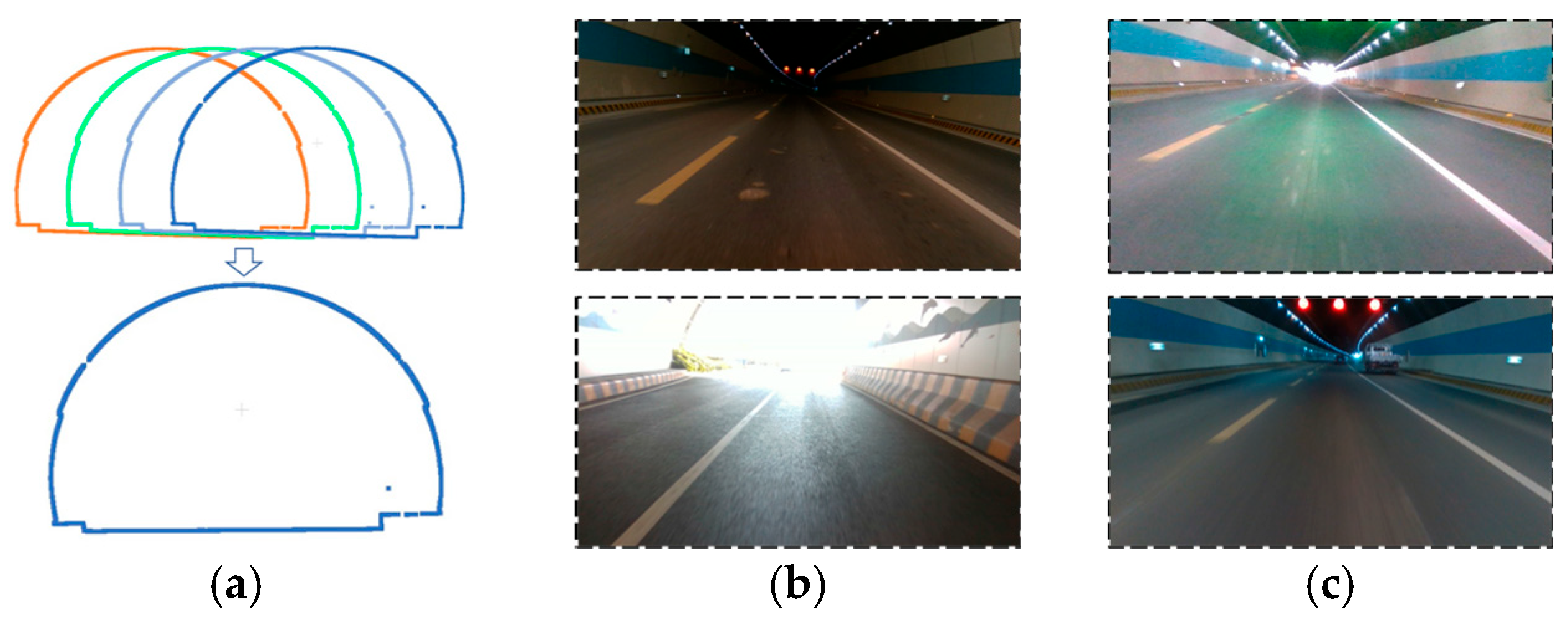
While an RTK-integrated SLAM (simultaneous localization and mapping) system, utilizing a low-cost consumer-level inertial sensor and a hybrid solid-state, narrow field-of-view LiDAR (light detection and ranging), can offer pose and map information in a geodetic coordinate frame, it still exhibits degraded performance in tunnel scenarios [2]. These environments are characterized by repetitive local structures, complex lighting variations, and extensive weak-texture areas as illustrated in Figure 1. These conditions hinder the ability of general SLAM systems to achieve accurate and robust pose estimation and map construction. Furthermore, due to signal loss, the unavailability of absolute RTK measurements within tunnels negatively impacts the overall performance of such systems. Although some research has investigated SLAM algorithms specifically tailored for tunnel environments [3,4], there remains a notable gap in the literature concerning low-cost SLAM solutions employing multi-source sensor fusion for these unique scenarios.

Figure 1. Challenging factors in tunnel environments. (a) Repetitive local structures, Different colored curves represent similar tunnel cross-sectional profiles at different locations (b) complex lighting changes, and (c) large weak-texture areas.

The intelligent exploitation and design of all available perception information remains an open challenge. Three key configurable modules that significantly affect accuracy and robustness are loop closure [5], quality control [6], and factor graph optimization [7]. In roadway tunnel inspection, configuring the inspection vehicle to follow a closed-loop route offers a beneficial constraint. For example, the inspection vehicle is designed to traverse one side of the tunnel first and then return along the opposite direction to complete the inspection process. However, ensuring robust loop closure remains difficult [8], as the high structural similarity between point cloud frames often leads to erroneous loop detections. However, semantic information offers a clear and intuitive description of specific tunnel sections, which need to be further explored.

A further limitation arises from the challenges of quality control inherent in processing the increased volume of potentially ambiguous sensor data. Effective quality control strategies must be specifically tailored to the distinct phases of the inspection process: tunnel entry, in-tunnel operation, and tunnel exit. During tunnel entry, the RTK receiver experiences signal degradation and a corresponding increase in drift error [9]. Within the tunnel, LiDAR and vision sensors are susceptible to the environmental challenges. Finally, upon exiting the tunnel, the RTK receiver reacquires satellite signals, allowing for drift mitigation. Designing and implementing a robust quality control strategy for multi-sensor integrated SLAM [10], one that comprehensively addresses the unique characteristics of each stage, remains a significant area for future research.

In the back-end factor graph optimization of the SLAM system, appropriate weights need to be assigned to all factors involved [11]. If the weights are set inappropriately, errors may be introduced into the trajectory estimation and map construction results. The construction method of weights and their related measurement values needs to be adjusted according to the specific application scenario.

With this motivation, we propose Tunnel-SLAM for multi-source fusion positioning and mapping in roadway tunnel scenarios, which is applicable to on-board road-way tunnel inspection and monitoring systems. The main contributions of this paper can be summarized as follows:

(1)

We propose a semantic-assisted hybrid coupling SLAM framework for LiDAR/vision/RTK/inertial sensors, offering a simple yet effective solution for roadway tunnel inspection. Compared to state-of-the-art SLAM methods, this framework significantly enhances positioning and mapping consistency.

(2)

Three componentized modules are integrated in this SLAM framework. A histogram-based semantic descriptor is designed to describe common infrastructures in roadway tunnels for loop closing detection; a quality control and stochastic model for various stages of roadway tunnel inspection is proposed to enhance SLAM feasibility. An adaptive factor graph optimization module is developed to involve LIO, RTK and loop closure factors to generate globally consistent trajectory estimation and mapping.

(3)

We collected data in various roadway tunnels using a low-cost hybrid solid-state LiDAR/vision/RTK/inertial on a self-assembled SLAM device. The effectiveness of the proposed framework was evaluated in real-world tunnel environments. Comparative experiments with state-of-the-art SLAM frameworks were conducted. Additionally, we performed ablation experiments to validate the performance of loop closure and quality control module.

The structure of the remainder of this paper is as follows: firstly, we discussed the related work, then sorted out the overall framework of the proposed algorithm, detailing the coordinate frame definition and transformation, LiDAR-inertial odometry, loop-closure detection and mapping, two-stage quality control on RTK, and backend optimization modules. Subsequently, the experimental platform was briefly introduced, and the experiments and corresponding analyses were conducted. Finally, we concluded the paper with future research direction.

2. Related Work

2.1. Multi-Sensor LiDAR Based SLAM Framework

With the development of various sensors in recent years, the evolution from single-source SLAM to multi-source SLAM has become a prominent trend. Mainstream SLAM algorithms are generally categorized into filtering-based and optimization-based methods. Within the filtering-based category, the LiDAR-only real-time odometry and mapping (LOAM) framework [12] was an early contribution, though its reliance solely on LiDAR data rendered it susceptible to drift. The LeGO-LOAM algorithm [13] addressed this limitation by integrating IMU data and a loop closure module into LOAM, leveraging ground plane information for optimization. These frameworks relied on mechanical LiDAR. Solid-state or semi-solid-state alternatives, such as Livox, offer enhanced reliability and faster scanning rates, albeit with a narrower field of view. LOAM-Livox [14] was a real-time, robust LiDAR LOAM algorithm specifically designed for small field-of-view and irregular sampling patterns, significantly promoting the adoption of cost-effective solid-state LiDAR and circumventing the traditional reliance on mechanical LiDAR. Furthermore, FAST-LIO2 [15] introduced a computationally efficient and robust tightly coupled LiDAR-inertial odometry framework, employing an efficient iterative Kalman filter (IKF) for direct raw point registration to the map, thereby enhancing mapping and localization efficiency without feature extraction. Optimization-based methods have also gained widespread adoption. LIO-SAM [16] was a tightly coupled LiDAR-inertial odometry through a sliding window approach. It incorporated RTK measurements, IMU data, and loop-closure features as factors for global optimization. The LVIO-SAM framework [17], building upon the LIO prototype [18] and further developed by LIO-SAM [16], integrated binocular cameras with LiDAR and IMU to achieve multi-sensor fusion odometry.

Visual measurements have also been explored to augment LiDAR-based SLAM or odometry. LIC-fusion 2.0 [19] realized efficient 6-DOF pose estimation through the multimodal sensor fusion of edge and face feature points, visual features, IMU data, and tracked LiDAR scans. It leveraged an efficient multi-state constraint Kalman filter (MSCKF) approach with a sliding window for planar feature tracking across multiple LiDAR scans. Super odometry [20] comprised visual odometry and LiDAR odometry components, providing attitude constraints for IMU and receiving motion predictions from IMU. R3LIVE [21] incorporated a LIO subsystem (FAST-LIO) that utilized LiDAR and inertial sensor measurements to construct map geometry, and a VIO subsystem that efficiently fused visual data by minimizing frame-to-map photometric errors. These modules collaborated to generate an accurate, dense, RGB-colored 3D map of the surrounding environment. LAMV-SLAM [22] combined LiDAR and visual data in the tracking thread to provide accurate depth values for visual features, estimating the real-scale camera transformation using fused LiDAR-visual data, followed by loop closure to minimize cumulative errors. Recent research, such as Refs. [23,24] has also focused on addressing LiDAR degradation through dynamic thresholds and adaptive settings. However, many of the aforementioned SLAM systems do not specifically address the challenges of tunnel environments, where a richer understanding of the surrounding environment is crucial. Furthermore, the design of a system with multiple modularity that can mitigate the impact of the degradation remains an open area of research.

Despite these advancements, applying general-purpose SLAM frameworks to roadway tunnels with low-cost sensors remains highly challenging. Tunnels often constitute geometrically degenerate environments, such as long and feature-sparse corridors, where methods struggle to maintain sufficient constraints along the travel direction. This issue is further aggravated by the limited field of view of low-cost solid-state LiDARs, which capture fewer distinctive structural features. Visual-augmented approaches also face significant difficulties in tunnel scenarios. Severe illumination variations at tunnel ingress and egress, together with repetitive visual patterns, frequently lead to tracking failures caused by perceptual aliasing. Moreover, existing loosely coupled multi-sensor fusion strategies often lack effective outlier rejection mechanisms for unstable GNSS signals in tunnel transition zones, resulting in abrupt trajectory jumps when erroneous RTK measurements are incorporated.

2.2. Loop-Closure Detection

In recent years, a variety of loop-closure detection algorithms with distinct descriptors for loop identification have been proposed. For instance, M2DP [25] projected a 3D point cloud onto multiple 2D planes, generating a compact 192-dimensional global representation. However, this projection necessitates the prior computation of the centroid and principal direction. SegMatch [26] offered robust performance in large-scale, unstructured environments, but required training and the representation of points within a global reference frame. Scan Context [27] encoded 3D scans into matrices, preserving absolute position information within each bin, and implemented a two-step search method for efficient and accurate matching. Successors to Scan Context, SSC [28] and SC++ [29], have further refined this approach. SC++ incorporated two sub-descriptors to enhance topological position retrieval and one degree-of-freedom semi-metric localization. SSC [28] integrated semantic information to improve descriptor representation. Similarly, GOSMatch [30] was a semantic-level approach that achieved reliable position identification by exploiting spatial relationships among semantic features to generate novel descriptors, and then employed a coarse-to-fine strategy for effective search. Deep learning-based Local 3D Depth (L3D) descriptors [31] offered a compact representation of point cloud patches learned from data. OverlapNet [32] utilized neural networks to analyze depth, normal vector, and intensity information from laser point clouds, estimating both the overlap and relative yaw angle between 3D scans. Overlap Transformer [33], a lightweight neural network, compressed LiDAR distance images into global descriptors. Semantic Graph [34] processes point clouds by preserving semantic and topological information through a semantic graph representation, facilitating efficient matching via a graph similarity network. STD [35] extracted key points from 3D point clouds and encoded them as stable triangular descriptors.

Despite these advancements, loop-closure detection in roadway tunnels remains challenging due to high structure similarity. The limited viewing field and sparse scanning lines of low-cost LiDAR systems further complicate the extraction of semantic objects from point clouds. A potential solution involves leveraging aligned LiDAR/vision data to provide additional semantic information, thereby enhancing loop-closure performance.

Despite the success of existing algorithms in general environments, loop-closure detection in roadway tunnels remains an open challenge. Geometry-centric methods (e.g., M2DP [25] and Scan Context [27]) are particularly vulnerable to perceptual aliasing in such scenarios, where highly repetitive structural elements (e.g., tunnel walls and lighting fixtures) produce nearly indistinguishable descriptors. Moreover, semantic approaches that rely solely on point clouds are often limited by the narrow field of view and sparse scan lines of low-cost LiDAR sensors, which hinder the reliable extraction of meaningful semantic objects.

2.3. Quality Control Strategies for GNSS-Denied Environments

While multiple sensor-based positioning and mapping has advanced considerably, challenges persist in mitigating the impact of environmental conditions, inadequate stochastic models, and flawed functional models on data quality. Robustness and accuracy in challenging environments are widely acknowledged as key technical hurdles [36]. Quality control strategies can be implemented from various perspectives, including pre-processing, stochastic model refinement, and functional model improvement. For example, UWNet module [37] enhances underwater image processing by extracting both local and global features, thereby improving tracking and loop-closure detection. Furthermore, a robust SLAM [38] aimed to create globally consistent maps by maximizing measurement inclusion through integrated consistency checking. To address the issue of moving objects, a geometric SLAM framework [39] integrating K-means clustering from epipolar constraints was proposed. In addition, a dual static map-point-detection strategy [40] has been proposed to exclude moving objects by analyzing both current and previous frames.

Adaptive stochastic models also offer a pathway to enhance estimation quality, as demonstrated by a stochastic sub-scene model [6] that analyzing GNSS signal characteristics and influencing factors in urban environments. In another SLAM system [41], the authors addressed rank deficit constraints in graph optimization through approximate null space analysis, enabling online map updates to accommodate trajectory changes. Additionally, DT-SLAM [42] incrementally tracks 2D features and estimates camera pose using matched features without baseline length constraints, delaying 3D triangulation until feature-specific baseline thresholds are met. These methods collectively enhance feature tracking, loop-closure detection, and back-end optimization to improve overall system robustness. However, while these advancements optimize pre-processing and estimation steps, they often lack comprehensive quality analysis and adaptive mechanisms specifically designed to handle the scenario of roadway tunnels.

3. System and Method

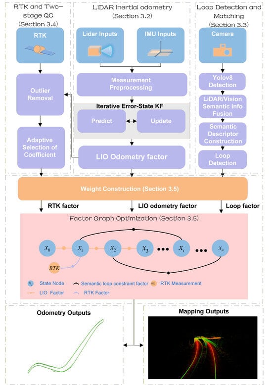
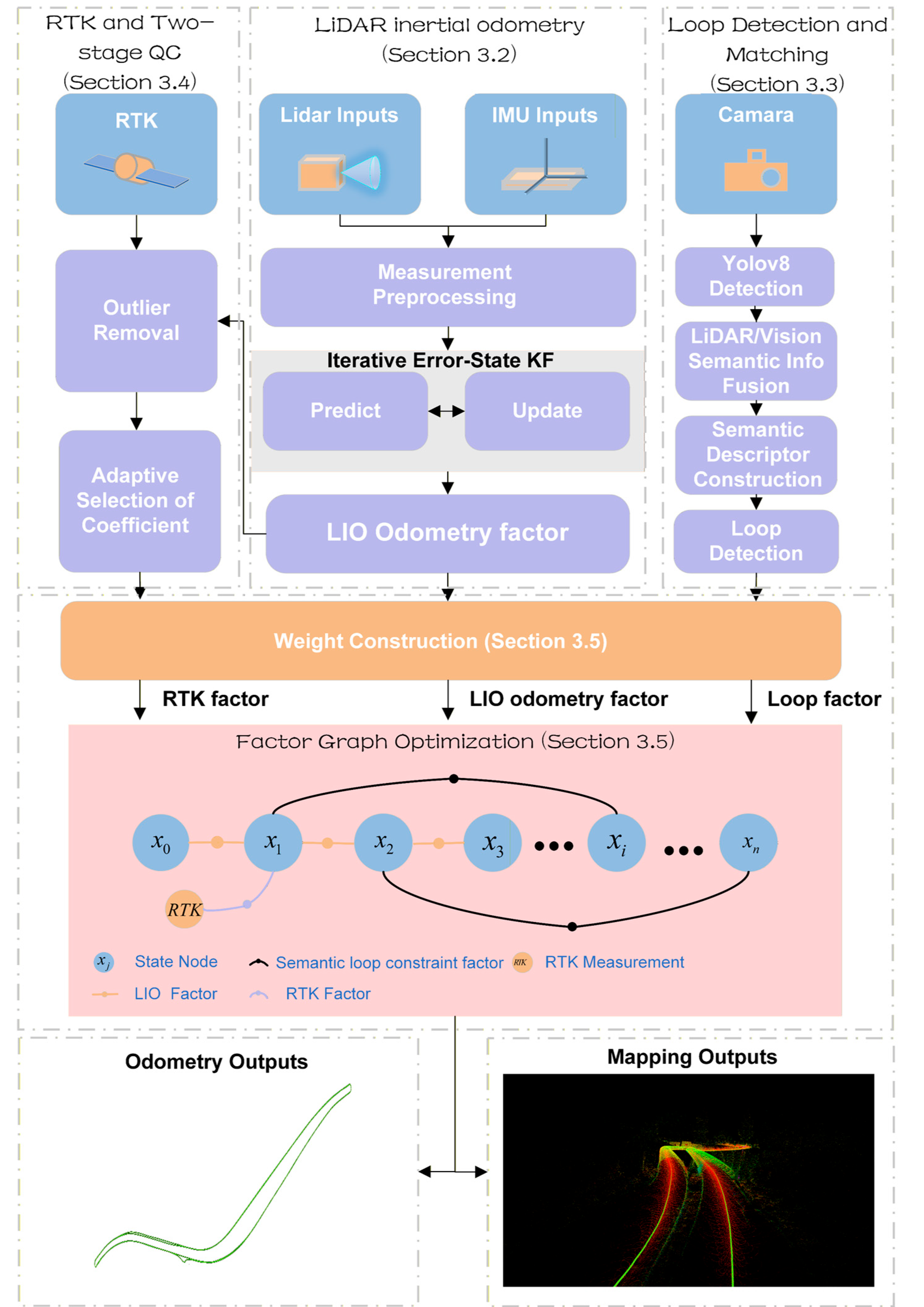
The overall framework of Tunnel-SLAM is illustrated in Figure 2. The LiDAR/IMU-based IESKF (iterative error state Kalman filter) serves as the primary odometry module, whose estimates are further refined through FGO (factor graph optimization). Rather than directly incorporating raw RTK and image measurements, factors derived from these measurements are integrated into the factor graph for global optimization. Finally, Tunnel-SLAM outputs both the positioning and mapping results. The main components can be described as follows:

Figure 2. Tunnel-SLAM framework.

• LiDAR-inertial odometry and mapping (Section 3.2). A tightly coupled IESKF fuses the LiDAR point cloud with IMU data, merging the newly scanned point cloud at the odometry rate and dynamically performing mapping. This module provides odometry factors for joint optimization.
• Loop detection and matching module (Section 3.3). The semantic loop module performs semantic object recognition on the input image, primarily for identifying tunnel appendages. It then fuses the semantic information from point cloud to construct SLD (semantic loop descriptor) for matching. Finally, it contributes the loop factor in joint optimization.
• Two-stage quality control on RTK module (Section 3.4). This module processes acquired RTK data to generate reliable positioning results after a two-stage processing including outlier detection and exclusion and noise covariance matrix reconstruction.
• Adaptive factor graph optimization (Section 3.5). This module incorporates LIO factor, RTK factor and loop factors derived from other modules, employs a key-frame strategy to construct the factor graph for global optimization, and outputs the globally optimized position estimate while updating the map.

3.1. Coordinate Definition

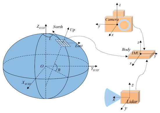
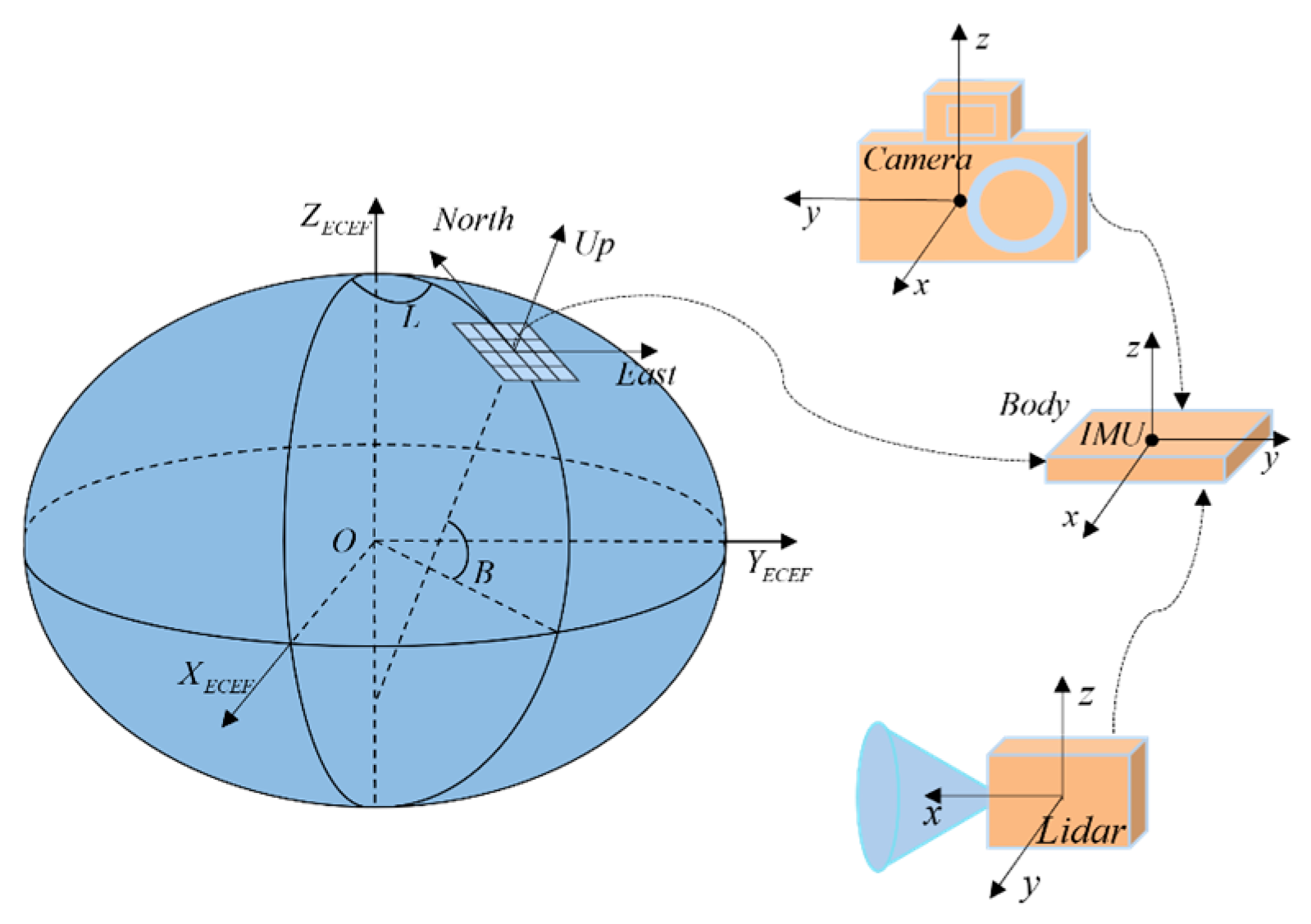
In Tunnel-SLAM, the WGS-84, Cartesian Earth-centered Earth-fixed (ECEF), local east-north-up (ENU), the local coordinate and the global coordinate frameworks are utilized. The relationship between the frameworks is shown in Figure 3:

Figure 3. Coordinate frame conversion.

For computational reasons, the IMU coordinate frame is designated as the global coordinate frame ${}^G\left(\cdot \right)$. Consequently, state estimation and map construction are performed and output within this global frame. The sensor suite of Tunnel-SLAM comprises a LiDAR, an IMU, a camera, and a RTK receiver, each possessing its own coordinate frame. These sensor frames are LiDAR coordinate frame ${\left(\cdot \right)}_L$, IMU coordinate frame ${\left(\cdot \right)}_{\mathrm{I}}$, Camera coordinate frame ${\left(\cdot \right)}_{\mathrm{C}}$, and RTK coordinate frame ${\left(\cdot \right)}_{\mathrm{g}}$ respectively. ${}^{\mathrm{b}}\left(\cdot \right)$ stands for the local coordinate frame of the whole device, which is aligned with the IMU coordinate frame. RTK raw positioning results are normalized to the geodetic coordinates under the WGS-84 coordinate system (latitude B, longitude L, height H), then it is transformed to the global coordinate system ${}^G\left(\cdot \right)$ through the ECEF frame ${}^{\mathrm{E}}\left(\cdot \right)$ and the ENU coordinate system ${}^{\mathrm{N}}\left(\cdot \right)$.

3.2. LiDAR/Inertial/Odometry

Tunnel-SLAM uses an iterative Kalman filter to tightly couple LiDAR measurements with inertial measurements, which is the main sub-system in the proposed SLAM framework. With reference to the state estimation section of FAST-LIO [15], we briefly describe the basic formulation and workflow of the filter below.

• Notations and Pose Representations. We use a rotation matrix ${\mathrm{R}}_{\mathrm{A}}^{\mathrm{B}}$ to represent the rotation from frame to frame and a translation vector ${\mathrm{p}}_{\mathrm{A}}^{\mathrm{B}}$ to represent the translation from frame to frame, ${\mathrm{T}}_{\mathrm{L}}^{\mathrm{I}}=\left({\mathrm{R}}_{\mathrm{L}}^{\mathrm{I}},{\mathrm{p}}_{\mathrm{L}}^{\mathrm{I}}\right)$ for the external parameter matrix between the LiDAR and the IMU.
• Kinematic Model. The continuous kinematic model can be discretized at the IMU sampling period $\Delta t$:

  $$x_{i+1}=x_i⊞\Delta tf\left(x_i,u_i,w_i\right)$$

  (1)

  where $i$ is the index of the IMU measurement and $⊞$ is the generalized plus sign, the function $f\left(\cdot \right)$, state $x$, input $u$ and noise $w$ are defined as follows

  $$x\triangleq {\left[{{}^{G}R}_I^T\hspace{1em}{}^{G}p_I^T\hspace{1em}{}^{G}V_I^T\hspace{1em}{b}_{\omega }^T\hspace{1em}{b}_a^T\hspace{1em}{}^{G}g^T\hspace{1em}{R}_L^{I^T}\hspace{1em}{p}_L^{I^T}\right]}^T$$

  (2)

  $$u\triangleq {\left[{\omega }_m^T\hspace{1em}{a}_m^T\right]}^T,w\triangleq {\left[n_{\omega }^T\hspace{1em}{n}_a^T\hspace{1em}{n}_{b\omega }^T\hspace{1em}{n}_{ba}^T\right]}^T$$

  (3)

  where ${{}^{G}R}_I,{{}^{G}p}_I,{{}^{G}V}_I$ are defined as the attitude, position and velocity of the IMU in the global coordinate system, ${}^{G}g$ is the gravity vector in the global coordinate system, $a_m$ and ${\omega }_m$ are the IMU acceleration measurements, and $n_{b\omega }$ are white noise in IMU measurements, $b_a$ and $b_{\omega }$ are the IMU biases modeling the random wandering process driven by $n_{ba}$ and $n_{b\omega }$, $R_L^{I^T}$ and $p_L^{I^T}$ represent the rotation and displacement from the LiDAR frame to the IMU frame, respectively.

  $$f\left(x,u,w\right)=\left[\begin{array}{c}\begin{array}{c}{\omega }_m-b_{\omega }-n_{\omega }\\ {}^{G}V_I+\left(1/2\right){(}^G{R}_I\left(a_m-b_a-n_a\right)+{}^{G}g\Delta t\end{array}\\ {}^{G}R_I\left(a_m-b_a-n_a\right)+{}^{G}g\\ n_{\omega }\\ n_a\\ 0_{3\times 1}\\ 0_{3\times 1}\\ 0_{3\times 1}\end{array}\right]$$

  (4)
• Measurement Model. Based on IMU measurements to compensate for the motion of the point cloud in a single scan, a planar fit is performed on the nearest neighbor points after de-distortion, and the measurement model is constructed as follows:

  $${}^{G}u_j^T{(}^G{T}_{Ik}{T}_L^I\left(p_{Lj}+n_{Lj}\right)-{}^{G}q_j=0$$

  (5)

  where ${}^{G}u_j^T$ is the normal vector of the fitting plane, ${}^{G}T_{\mathit{Ik}}$ is the LiDAR’s position in the global coordinate frame, ${}^{G}q_j$ is a point in the fitting plane, $T_L^I$ is the external reference matrix, $p_{Lj}$ is a point in the LiDAR system for the point cloud indexed by, and $n_{Lj}$ is the LiDAR measurement noise.

Based on the state propagation model and the measurement model, the iterative Kalman filter (IKF) is applied for estimation. This process involves IMU forward propagation, residual computation and iterative state updating. Finally it outputs the estimated poses. The estimated poses are used as the factor in FGO. Incremental mapping is then performed based on the estimated poses.

3.3. Semantic-Assisted Loop Detection and Matching Module

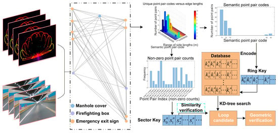
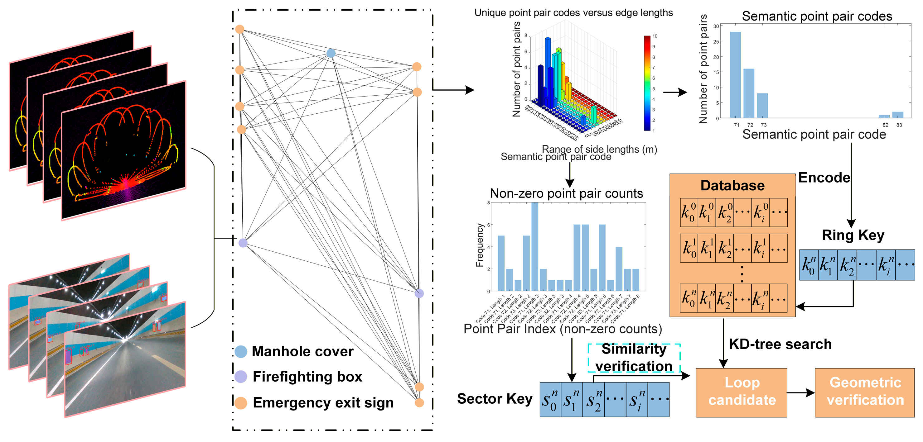
The loop detection flow, which is a key module in Tunnel-SLAM, is illustrated in Figure 4. Each tunnel appurtenance (e.g., traffic signs, fire boxes, etc.) can be detected by images and its distance can be calculated by the corresponding point clouds. The appurtenances are represented by a graph, which describes a certain area of tunnels (e.g., A 50 m-long section). How to describe the graph and find the most similar graph is described in the following sub-sections.

Figure 4. Flow of generating semantic loop closure descriptors generation and matching.

• Semantic Loop Descriptors. Given the point cloud from a keyframe, images with corresponding timestamps are processed using YOLOv8 [43], this process identifies various tunnel appurtenances, identifying 15 semantic classes including fans, illuminated lamps, traffic signs, emergency exit, emergency indicator lights, fire boxes, manhole covers, trash cans, triangular signages, rectangular signages, circular signages, fire hydrants, navigation signages, traffic surveillance cameras, and street lamps. These semantic categories are predetermined during model training.

The resulting recognition data is mapped onto the point cloud. Since these objects are detected in multiple frames, a multi-target tracking algorithm is employed to track and cluster semantic points of these objects as illustrated in Algorithm 1. This algorithm extracts high-confidence semantic points by fusing image and LiDAR data. The point cloud is projected onto 2D detection bounding boxes, and the valid point closest to the center of each box is selected as the semantic anchor point. Leveraging label consistency and coordinate transformations across multiple frames, these semantic points are tracked and clustered. Therefore it effectively extracts anchor points corresponding to specific tunnel appurtenances. Each semantic point, representing an individual instance, is treated as a single node in a graph, facilitating the construction of a semantic graph for instantiated objects (e.g., exhaust fans, fire hydrants). Each node in this graph contains the global coordinates of the object instance and its associated semantic label. This algorithm extracts high-confidence semantic points in keyframes by fusing image and LiDAR data.

Algorithm 1: Semantic Point Extraction

$\mathbf{Input}: 2\mathrm{D} \mathrm{detection} \mathrm{boxes} B_t$$\mathrm{with} \mathrm{timestamp} t_c$$;$ $\mathrm{LiDAR} \mathrm{point} \mathrm{cloud} {\mathcal{P}}_{\mathcal{t}}$$\mathrm{at} \mathrm{keyframe} t_k$; $\mathrm{Keyframe} \mathrm{poses} T_{k-1}$$, T_k$; Camera intrinsic and distortion model; $\mathrm{Extrinsic} \mathrm{parameters} T_{CL}$$, T_{IL}$; $\mathbf{Output}: \mathrm{Semantic} \mathrm{base} \mathrm{point} \mathrm{set} S_k$ $\mathbf{Variable}: \mathsf{\gamma }$$: \mathrm{Time} \mathrm{interpolation} \mathrm{factor} \mathrm{for} \mathrm{sensor} \mathrm{pose} \mathrm{synchronization}; T_c$$: \mathrm{Interpolated} \mathrm{camera} \mathrm{pose} \mathrm{at} \mathrm{image} \mathrm{time}; R_{CL}$$,t_{CL}$$: \mathrm{rotation} \mathrm{and} \mathrm{translation} \mathrm{of} \mathrm{the} \mathrm{LiDAR}\text{-}\mathrm{to}\text{-}\mathrm{camera} \mathrm{extrinsic} \mathrm{calibration}; \mathsf{\pi }\left(\cdot \right)$$: \mathrm{Camera} \mathrm{projection} \mathrm{model} \mathrm{mapping} 3\mathrm{D} \mathrm{points} \mathrm{to} \mathrm{the} 2\mathrm{D} \mathrm{image} \mathrm{plane}; p_L^j$: the $j$$\text{-}\mathrm{th} \mathrm{LiDAR} \mathrm{point} \mathrm{expressed} \mathrm{in} \mathrm{the} \mathrm{LiDAR} \mathrm{frame}; u_j$: The projection of the $j$$\text{-}\mathrm{th} \mathrm{LiDAR} \mathrm{point} \mathrm{onto} \mathrm{the} \mathrm{image} \mathrm{plane}; c_i^j$: Geometric center of the $i$$\text{-}\mathrm{th} \mathrm{detection} \mathrm{box} b_t^i$$; d$$,d_{min}$$: \mathrm{Current} \mathrm{and} \mathrm{minimum} \mathrm{Euclidean} \mathrm{distance} \mathrm{between} \mathrm{a} \mathrm{projected} \mathrm{point} \mathrm{and} \mathrm{the} \mathrm{box} \mathrm{center}; d_{max}$$: \mathrm{Maximum} \mathrm{valid} \mathrm{LiDAR} \mathrm{range} \mathrm{for} \mathrm{semantic} \mathrm{association}; p_k^{i*}$$: \mathrm{The} \mathrm{candidate} \mathrm{semantic} \mathrm{base} \mathrm{point} (\mathrm{closest} \mathrm{to} \mathrm{the} \mathrm{box} \mathrm{center}) \mathrm{for} \mathrm{a} \mathrm{specific} \mathrm{detection} \mathrm{box}; p_{k\to k-1}^{i*}$$: \mathrm{The} \mathrm{semantic} \mathrm{base} \mathrm{point} \mathrm{from} \mathrm{keyframe} k$$\mathrm{transformed} \mathrm{into} \mathrm{the} \mathrm{coordinate} \mathrm{frame} \mathrm{of} \mathrm{keyframe} k-1$$; \mathsf{\tau }$: Confidence threshold for filtering valid detection boxes. 1: Compute interpolation factor $\mathsf{\gamma }\leftarrow {\displaystyle \frac{t_c-t_{k-1}}{t_k-t_{k-1}}}$ 2: $\mathrm{Estimate} \mathrm{sensor} \mathrm{pose} \mathrm{at} \mathrm{image} \mathrm{time} T_c\leftarrow T_k\cdot \exp \left(\mathsf{\gamma }\cdot \log \left(T_k^{-1}\cdot T_{k-1}\right)\right)$ 3: $\mathrm{for} \mathrm{each} \mathrm{point} p_L\in {\mathcal{P}}_{\mathcal{t}}$ do 4:   ${ p}_c\leftarrow R_{CL}{p}_L+t_{CL}$ 5:   $\mathrm{if} z_c>0$ then 6:    $u\leftarrow \mathsf{\pi }\left(p_c\right)$ 7: $\mathrm{for} \mathrm{each} \mathrm{detection} \mathrm{box} b_t^i\in B_t$ do 8:   $\mathrm{if} \mathrm{confidence} (b_t^i$$) \text{<} \mathsf{\tau }$ or label is ignored then 9:     continue 10:   $\mathrm{Compute} \mathrm{box} \mathrm{center} c_t^i$ 11:   $\mathrm{Initialize} \mathrm{minimum} \mathrm{distance} d_{min}$ 12:   $\mathrm{For} \mathrm{each} \mathrm{projected} \mathrm{point} u_j$$\mathrm{inside} b_t^i$ do 13:    $\mathrm{if} \Vert p_L^j\Vert <d_{max}$ then 14:     $d\leftarrow \Vert u_j-c_t^i\Vert$ 15:     $\mathrm{if} d<d_{min}$ then 16:     $d_{min}\leftarrow d$ 17:     $p_k^{i\mathrm{*}}\leftarrow p_L^j$ 18:    $\mathrm{if} \mathrm{valid} p_k^{i\mathrm{*}}$ exists then 19:     $\mathrm{Add} p_k^{i\mathrm{*}}$$\mathrm{to} S_t$ 20: $\mathrm{if} \mathrm{previous} \mathrm{semantic} \mathrm{set} S_{t-1}$ exists then 21: $\mathrm{for} \mathrm{each} p_k^{i\mathrm{*}}\in S_k$ do 22: $p_{k\to k-1}^{i\mathrm{*}}\leftarrow T_{k-1}^{-1}{T}_k{p}_k^{i\mathrm{*}}$ 23:  $\mathrm{if} \mathrm{projected} \mathrm{point} \mathrm{lies} \mathrm{in} \mathrm{a} \mathrm{box} b_{t-1}^j$ with same label then 24:  $S_k\leftarrow S_k\setminus \left\{p_k^{i\mathrm{*}}\right\}$ 25: $\mathrm{return} S_k$

Within the roadway tunnel environment, a sliding window is employed to traverse the semantic nodes. The sliding window must contain at least a minimum number of nodes $N_{min}\ge 10$, and the Euclidean distance between any two nodes within the window must not exceed a predefined threshold $D_{max} \le 50$ m. A fully connected, undirected graph is then constructed using these nodes, where each edge is characterized by the semantic labels of the two connected nodes and the edge length. This process yields a set of node pairs and associated graph edges derived from the overarching semantic graph.

Having established the semantic graph, a semantic descriptor is designed to facilitate subsequent descriptor similarity matching. The node pairs within the semantic graph are first classified and encoded. For example, a node pair with semantic labels $l_1$ and $l_2$ is mapped to a unique integer code using a triangular-number-based encoding scheme.

$$code={\displaystyle \frac{l_{max}\left(l_{max}+1\right)}{2}}+l_{min}$$

(6)

where $l_{min}=\min \left(l_1,l_2\right)$ and $l_{max}=\max \left(l_1,l_2\right)$. This ensures a consistent and repetition-free integer representation for unordered semantic pairs. For example, consider a node pair with label $l_1=3$. (e.g., “traffic sign”) and $l_2=9$ (e.g., “fire box”). we compute $l_{\mathrm{m}\mathrm{i}\mathrm{n}}=\min \left(\mathrm{3,9}\right)=3$ and $l_{max}=\max \left(\mathrm{3,9}\right)=9$. The corresponding code is given by 48.

The lengths of all graph edges are then quantized to construct a 2D histogram-based semantic descriptor. Each edge is jointly binned by its length (uniformly discretized into 10 bins over [0, 50] m) and its semantic type encoded as a unique integer from the unordered node label pair. For example, an edge of length 12.4 m between labels 3 and 7 maps to the bin (length bin 2, semantic index 31).

• Semantic Descriptor Search and Matching. A primary limitation of the semantic descriptor is the inefficient memory usage caused by sparse descriptor arising from zero entries. This occurs because edge lengths may not span all quantization intervals.

To facilitate efficient loop closure retrieval, we introduce a novel global descriptor and a two-phase search method inspired by Scan Context [27]. First, a ring key comprising head and tail elements is generated. The head encodes the occurrence of semantic point pair types, while the tail records their corresponding frequencies. For example, if the head contains encoded labels such as [1,3,7] representing distinct semantic pairs (e.g., traffic sign-lamp, traffic sign-rectangular signages, traffic sign-circular signages), and the tail holds their observed frequencies [5,10,12], the resulting ring key is formed by concatenating these two parts into a fixed-length vector. With denoting the descriptor index $n$ in element $K_i^n$, this ring key is stored in a database. Once the number of stored ring keys reaches a predefined threshold, a k-d tree is constructed to enable efficient KNN search [44]. The newly generated ring key then undergoes a KNN search to identify similar loop closure candidates with the number of candidates being customizable. Subsequently, the corresponding sector key undergoes similarity computation based on the index. The sector key comprises a vector of edge lengths associated with the candidate loop closures, where each element represents the point pair length derived from the 2D histogram frequency. If the similarity score exceeds a predefined threshold, geometric verification between the current scan and the local map is performed, and the resulting loop-closure constraints are integrated into the back-end optimization module.

3.4. Two-Stage Quality Control on RTK

RTK results and IMU measurements are loosely coupled to provide global constraints for the system. The RTK positioning results, given in geodetic coordinates under the WGS-84 coordinate system (latitude $B$, longitude $L$, height $H$), are transformed into the ENU coordinate system, as detailed in [45]. With extrinsic calibration using hand–eye calibration, the RTK positioning results are then integrated into the global coordinate system. A constant time offset is applied between the clocks of IMU and RTK to achieve unified time reference. Given the RTK output frequency of 10 Hz, a time threshold is applied to identify the nearest RTK measurement for each keyframe, after which linear interpolation is employed to softly synchronize the RTK data with the keyframes.

In roadway tunnel scenarios, RTK positioning faces complete signal loss inside the tunnel and substantial jumps in the estimated position when entering or exiting the tunnel. To address these issues, anomalous positioning results must be accurately rejected. We propose a hierarchical outlier detection strategy comprising a directional pre-check followed by a B-spline trajectory verification.

• Directional consistency Pre-check. LiDAR-inertial odometry, which provides precise local position estimates, is employed to filter out such anomalous RTK localization results. The position coordinates ${(}^G{p}_{pre},{{}^{G}p}_{cur})$ of the two keyframes before and after are used to form the direction vector ${\overrightarrow{n}}_{lio}$, each keyframe is associated with a RTK positioning result (if available) based on the uniform time base. The associated RTK positioning results of the same two frames are used to form the direction vector ${\overrightarrow{n}}_{rtk}$, and cosine similarity is employed to quantify the directional similarity between the two vectors.

  $$\cos \left({\overrightarrow{n}}_{lio},{\overrightarrow{n}}_{rtk}\right)={\displaystyle \frac{{\overrightarrow{n}}_{lio}\cdot {\overrightarrow{n}}_{rtk}}{‖{\overrightarrow{n}}_{lio}‖‖{\overrightarrow{n}}_{rtk}‖}}$$

  (7)

  If $\cos \left({\overrightarrow{n}}_{lio},{\overrightarrow{n}}_{rtk}\right)$ is less than a preset threshold of 0.96, the RTK positioning result is considered unreliable and thus rejected.
• B-Spline Trajectory Verification. RTK measurements that pass the directional pre-check undergo a secondary, fine-grained assessment using cubic B-spline interpolation to evaluate temporal consistency. A sliding window of the five most recent valid poses is maintained, and outliers are identified through a two-step residual analysis, as illustrated in Algorithm 2. Anomaly detection is performed on RTK positioning data within a sliding window by fitting the trajectory with cubic B-splines and evaluating residuals. A B-spline is first fitted to all points in the window to assess overall trajectory consistency; if any residual exceeds a dynamically adjusted threshold, the window is flagged as anomalous. The latest point is then predicted using preceding points, and is marked as an anomaly if either the temporal extrapolation is excessive or its residual exceeds the threshold.

Algorithm 2: B-Spline Trajectory Verification for RTK results

$\mathbf{Input}: \mathrm{A} \mathrm{sliding} \mathrm{window} \mathrm{of} \mathrm{RTK} \mathrm{measurements} \{\left(p_i,t_i\right){\}}_{i=0}^4$$, \mathrm{where} p_i\in R^3$$\mathrm{denotes} \mathrm{the} \mathrm{RTK} \mathrm{position} \mathrm{at} \mathrm{time} t_i$$; \mathrm{an} \mathrm{optional} \mathrm{residual} \mathrm{threshold} \mathsf{\tau }$ $\mathbf{Output}: \mathrm{is}\text{\_}\mathrm{outlier}\in \{\mathrm{true},\mathrm{false}\}$ $\mathbf{Variable}: s_i,u_i$: Time parameters normalized to [0, 1]; $r_i$: residual for each RTK point; ${\mathsf{\tau }}_L,{\mathsf{\tau }}_W$: Threshold for window and latest-point checks;$e_i$: Residual between actual and predicted position at time $i$$; \overline{r}$$: \mathrm{average} \mathrm{residuals}; \overline{e}$$: \mathrm{Mean} \mathrm{of} \mathrm{previous} \mathrm{residuals}; S\left(\cdot \right)$: Cubic approximating B-spline function; window_outlier, is_outlier: Boolean flags (initialized as false) 1: $\mathrm{Extract} \mathrm{RTK} \mathrm{position} p_i\in R^3$$\mathrm{and} \mathrm{timestamps} t_i$$\mathrm{for} i = 0 \dots 4$ 2: $s_i\leftarrow \left(t_i-t_0\right)/\left(t_4-t_0\right)$ // normalize time to [0, 1] 3: $S_5\left(s\right)\leftarrow \mathrm{Construct} \mathrm{Cubic} \mathrm{Approximating} \mathrm{BSpline} \left(p_0,\dots ,p_4\right)$ 4: $\widehat{p_i}\leftarrow S_5\left(s_i\right)$$//\mathrm{predicted} \mathrm{position} \mathrm{at} s_i$ 5: $r_i\leftarrow \Vert p_i-\widehat{p_i}\Vert$ // calculate residuals 6: $\overline{r}\leftarrow {\displaystyle \frac{1}{5}}{\sum }_{i=0}^4{r}_i$ // average residual 7: ${\tau }_W\leftarrow \left\{\begin{array}{c}\tau \hspace{1em}\mathrm{i}\mathrm{f} \tau >0\\ 2\overline{r}\hspace{1em}\mathrm{o}\mathrm{t}\mathrm{h}\mathrm{e}\mathrm{r}\mathrm{w}\mathrm{i}\mathrm{s}\mathrm{e}\end{array}\right.$ 8: $\mathrm{if} \mathrm{any} r_i>{\tau }_W$ then 9:  window_outlier  $\leftarrow$ true 10: $S_4\left(u\right)\leftarrow \mathrm{Construct} \mathrm{Cubic} \mathrm{Approximating} \mathrm{BSpline} \left(p_0,\dots ,p_3\right)$ // fit first 4 points 11: $u_i\leftarrow \left(t_i-t_0\right)/\left(t_3-t_0\right)$$\mathrm{for} i=0\dots 3$ 12: $u_4\leftarrow \left(t_4-t_0\right)/\left(t_3-t_0\right)$ 13: $\mathrm{if} u_4>1+$ time_extrapolation_limit then //default: 0.5 14:  return true 15: ${\tilde{p}}_4\leftarrow S_4\left(u_4\right)$ // predict latest RTK position 16: $e_4\leftarrow \Vert p_4-{\tilde{p}}_4\Vert$ // latest residual 17: $\overline{e}\leftarrow {\displaystyle \frac{1}{4}}{\sum }_{i=0}^3{e}_i$ // mean of previous residuals 18: ${\mathsf{\tau }}_{\mathrm{L}}\leftarrow \left\{\begin{array}{c}\tau \\ 2\overline{\mathrm{e}}\end{array}\right.$ // latest-point threshold 19: $\mathrm{if} e_4>{\tau }_L$ or window_outlier then 20:  is_outlier $\leftarrow$ true 21: return is_outlier

After erroneous RTK positioning results are accurately rejected, its results can be used in the following adaptive FGO process.

3.5. Adaptive Factor Graph Optimization

If abnormal measurements are included in FGO, the trajectory will experience significant drift, thereby degrading the global consistency. In this module, we use adaptive factor graphs to address weighting issues in roadway tunnel scenarios. These graphs assign different weights based on different scenarios.

• LiDAR-Inertial Odometry Factor. Degradation direction detection is employed to assess the quality of the estimates for 6 DoF (degree of freedom) pose estimation. By linearizing the point-to-plane measurement equation in [15], we obtain:

  $$z = Hx + v$$

  (8)

  where $z$ is the measurement vector, $H$ is the Jacobian matrix of the LiDAR measurement model, $x\in SO\left(3\right)\times R^3$ is the status vector, and $v\in \mathcal{N}\left(0,R\right)$ represents measurement noise. The LiDAR measurement equations were transformed using the weighted linear least squares method to obtain:

  $$H^T{R}^{-1}H\widehat{x}=H^T{R}^{-1}z$$

  (9)

  First, redefine the LiDAR measurement linearization equation:

  $$H_I=H^T{R}^{-1}H,\tilde{z}=H^T{R}^{-1}z$$

  (10)

  $$H_I\widehat{x}=\tilde{z}$$

  (11)

  where H is the $m \times 6$ dimensional Jacobian matrix with respect to the measurement model in [15], $m$ is the number of point-to-plane measurement equations, and $R$ is the covariance matrix of the LiDAR measurement noise.

The matrix $H_I$ is expressed in terms of chunked matrices as follows:

$$H_I=\left[\begin{array}{cc}{H}_{rr}& H_{rt}\\ H_{tr}& H_{tt}\end{array}\right]$$

(12)

where $H_{rr}$,${ H}_{rt}$,$H_{tr}$,$H_{tt}$ denote the rotation-rotation (rr), rotation-translation (rt), translation-rotation (tr), and translation-translation (tt) blocks of the $H_I$, respectively. The goal is to determine the estimation accuracy in terms of rotation and translation using the method described in [46], thereby assigning different weights to obtain the covariance matrix of the state variables $\mathsf{\Sigma }$ as follows:

$$\mathsf{\Sigma }=H_I^{-1}=\left[\begin{array}{cc}{\mathsf{\Sigma }}_{rr}& {\mathsf{\Sigma }}_{rt}\\ {\mathsf{\Sigma }}_{tr}& {\mathsf{\Sigma }}_{tt}\end{array}\right]$$

(13)

$${\mathsf{\Sigma }}_{rr}={\left(H_{rr}-H_{rt}{H}_{tt}^{-1}{H}_{tr}\right)}^{-1}$$

(14)

$${\mathsf{\Sigma }}_{tt}={\left(H_{tt}-H_{tr}{H}_{rr}^{-1}{H}_{rt}\right)}^{-1}$$

(15)

Eigenvalue decomposition is obtained for ${\mathsf{\Sigma }}_{rr}$ and ${\mathsf{\Sigma }}_{tt}$:

$${\mathsf{\Sigma }}_{rr}=V_r\left[\begin{array}{cc}{\lambda }_{r1}& \begin{array}{cc}0& 0\end{array}\\ \begin{array}{c}0\\ 0\end{array}& \begin{array}{cc}{\lambda }_{r2}& 0\\ 0& {\lambda }_{r3}\end{array}\end{array}\right]V_r^T$$

(16)

$${\mathsf{\Sigma }}_{tt}=V_t\left[\begin{array}{cc}{\lambda }_{t1}& \begin{array}{cc}0& 0\end{array}\\ \begin{array}{c}0\\ 0\end{array}& \begin{array}{cc}{\lambda }_{t2}& 0\\ 0& {\lambda }_{t3}\end{array}\end{array}\right]V_t^T$$

(17)

Here the unit of ${\mathsf{\lambda }}_{ri}$ $\left(i=\mathrm{1,2},3\right)$ is the square of the angular unit $\left(\mathrm{r}\mathrm{a}{\mathrm{d}}^2\right)$, the unit of ${\lambda }_{tj} \left(j=\mathrm{1,2},3\right)$ is the square of the unit of length, ${\lambda }_{ri}$ and ${\lambda }_{tj}$ are able to determine more accurately the degree of degradation of the respective directions they represent.

We use $\{{\omega }_r,{\omega }_t\}$ to characterize the reliability of LiDAR-inertial odometry rotation and translation estimates.

$${\omega }_r=c_1\cdot {\displaystyle \frac{1}{\max \left({\lambda }_{r1},{\lambda }_{r2},{\lambda }_{r3}\right)}},{\omega }_t=c_2\cdot {\displaystyle \frac{1}{\min \left({\lambda }_{t1},{\lambda }_{t2},{\lambda }_{t3}\right)}}$$

(18)

where $c_1,c_2$ is a coefficient that is modified based on the scenario. We define $W_{lio}$ as a $6\times 6$ diagonal matrix, $W_{lio}=diag\left({\omega }_r\hspace{1em}{\omega }_r\hspace{1em}{\omega }_r\hspace{1em}{\omega }_t\hspace{1em}{\omega }_t\hspace{1em}{\omega }_t\right)$. In the scenarios we are targeting, there are two main categories: inside the tunnel and outside the tunnel. In the tunnel interior, the coefficients $c_1$ and $c_2$ are set to ${10}^{-8}$ and ${10}^{-6}$, respectively. In contrast, for the exterior tunnel environment, $c_1$ and $c_2$ are adjusted to${ 10}^{-6}$ and ${10}^{-4}$, respectively.

By integrating RTK data, LiDAR measurements, and IMU measurements, we can determine the current state of the carrier. The availability of RTK positioning results, after removing outliers, can be used to assess which of the aforementioned scenarios the carrier is in, as illustrated in Algorithm 3, to determine the appropriate constants, where these constants are obtained empirically.

Algorithm 3: Adaptive Selection of coefficient

Input: RTK measurements $Z_{rtk}$, LiDAR measurement $Z_{lidar}$, IMU measurement $Z_{imu}$ Output: $W_c=\{c_1,c_2\}$ Variable: RTK positioning results $P_{rtk}$, LiDAR-inertial odometry results $O_{lio}$. 1: $P_{rtk},O_{lio}\leftarrow CalculateAndExtract\left(Z_{rtk},Z_{lidar},Z_{imu}\right)$ 2: $S_{cur}\leftarrow JudgeScenario\left(P_{rtk},O_{lio}\right)$ 3: if $S_{cur}$ is Inside Tunnel then 4:  $W_c\leftarrow Param{s}_{tunnel}$ 5: else 6:  $W_c\leftarrow Param{s}_{outside}$ 7: end 8: return $W_c$

And the a priori residual of the LiDAR-inertial odometry can be expressed as:

$${\delta }_{lio}=\left[\begin{array}{c}\log \left({\left({\widehat{R}}_k^{lio}\right)}^{-1}{R}_k\right)\\ p_k-{\widehat{p}}_k^{lio}\end{array}\right]$$

(19)

where $\left({\widehat{R}}_k^{lio},{\widehat{p}}_k^{lio}\right)$ is the pose output by LiDAR-inertial odometry at keyframe, $k$. denotes the state estimate in the update phase and $x_{k|k-1}$ denotes the prediction estimate in the prediction phase.

• RTK Factor. Given the loose coupling at the RTK position output level and the absence of an associated noise covariance matrix, a suitable weighting matrix is essential for accurate estimation in FGO. We propose an adaptive RTK factor weighting strategy based on joint temporal and spatial consistency evaluation. Tunnel-SLAM dynamically adjusts the confidence of each RTK measurement by assessing its agreement with both recent RTK history and an independent local odometry estimate. The temporal inconsistency is defined as:

  $$d_{temporal}={\displaystyle \frac{‖p_t^{rtk}-{\widehat{y}}_t‖}{{\sigma }_{temp}}},\hspace{1em}{\widehat{y}}_t=S\left(p_{t-4:t-1}^{rtk}\right)$$

  (20)

  Let $p_t^{rtk}\in R^3$ denote the position measurement at $t$, ${\widehat{y}}_t$ denotes the extrapolated RTK position at time $t$, $S\left(\cdot \right)$ denotes the prediction function that extrapolates historical RTK positions using a cubic B-spline model. ${\sigma }_{temp}$ represents the expected short-term smoothness error of the B-spline model.

Let $p_t^{lio}$ denote the position estimated by LiDAR-inertial odometry at time $t$ in the same global reference frame. The spatial inconsistency is defined as:

$$d_{spatial}={\displaystyle \frac{‖p_t^{rtk}-p_t^{lio}‖}{{\sigma }_{lio}}}$$

(21)

Here, ${\sigma }_{lio}$ is the standard deviation of LiDAR-inertial odometry, derived from its covariance matrix.

The overall inconsistency score is computed as a weighted combination of temporal and spatial inconsistency terms:

$$D_t={\omega }_1{d}_{temporal}+{\omega }_2{d}_{spatial}$$

(22)

$$Q_{rtk}={\sigma }_{base}^2\cdot \min \left(f_{\mathrm{m}\mathrm{a}\mathrm{x}},\mathrm{e}\mathrm{x}\mathrm{p}\left({\displaystyle \frac{D_t}{D_0}}\right)\right)\cdot I$$

(23)

$$W_{rtk}=Q_{rtk}^{-1}$$

(24)

The weight coefficients satisfy ${\omega }_1+{\omega }_2=1$. In our system, we set ${\omega }_1=0.6$ and ${\omega }_2=0.4$, Here, ${\sigma }_{base}^2$ denotes the nominal RTK variance, $D_0$ controls the sensitivity of the scaling function, and $f_{max}=100$ is used to prevent numerical instability caused by excessively large residuals.

The RTK residuals can be expressed as:

$${\delta }_{rtk}=E_{lio}-P_{rtk}$$

(25)

Here, $E_{lio}$ denotes the LiDAR-inertial odometry estimate, and $P_{rtk}$ denotes the RTK position measurement

• Loop Factor. The relative pose constraints between loop-matching pair indices obtained by the loop detection module are derived through scan-to-local map matching. The residual equation for constructing the loop constraints is:

  $${\delta }_{loop}=T_{rel}\left(T_i{\xi }_i\right)-T_j{\xi }_j$$

  (26)

${\delta }_{loop}$ is the residual obtained from scan-to-local map matching, $\left({\xi }_i,{\xi }_j\right)$ are corresponding matched points from the source and target point clouds, $T_i$ and $T_j$ are the global poses of the source and target point clouds estimated by LiDAR-inertial odometry, respectively, and $T_{rel}$ is the loop closure relative pose constraint obtained through scan-to-local map matching.

Regarding the loop-closure constraints in Equation (27), the weight matrix $W_{loop}$ is constructed as a $6\times 6$ diagonal matrix to balance the global consistency within the joint optimization. Specifically, we employ a constant Gaussian noise model where $W_{loop}=diag{\left({\sigma }_r^2\hspace{1em}{\sigma }_r^2\hspace{1em}{\sigma }_r^2\hspace{1em}{\sigma }_t^2\hspace{1em}{\sigma }_t^2\hspace{1em}{\sigma }_t^2\right)}^{-1}$. The variances for the rotation and translation components are empirically set to ${\sigma }_r^2=0.2$ and ${\sigma }_t^2=0.05$, respectively.

With the aforementioned factors, joint optimization is performed as follows:

$$\arg \min \left(\sum |{\delta }_{lio}{|}^2{W}_{lio}+\sum |{\delta }_{rtk}{|}^2{W}_{rtk}+\sum |{\delta }_{loop}{|}^2{W}_{loop}\right)$$

(27)

where ${\delta }_{lio}$, ${\delta }_{rtk}$ and ${\delta }_{loop}$ denote the residuals from LiDAR-inertial odometry, RTK, and loop-closure constraints, respectively; $W_{lio}$, $W_{rtk}$ and$W_{loop}$ denote their corresponding weight matrices.

4. Experiment and Results

In this section, we validate Tunnel-SLAM and compare it with other state-of-the-art methods using datasets collected by a low-cost SLAM device, and conduct ablation experiments and time consumption tests to verify the effectiveness and efficiency of the proposed modules. All experiments are performed on a PC equipped with an Intel i5-12400F @ 2.5 GHz with 16 GB memory.

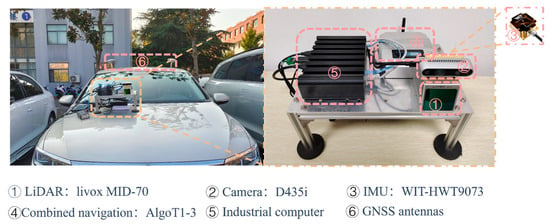
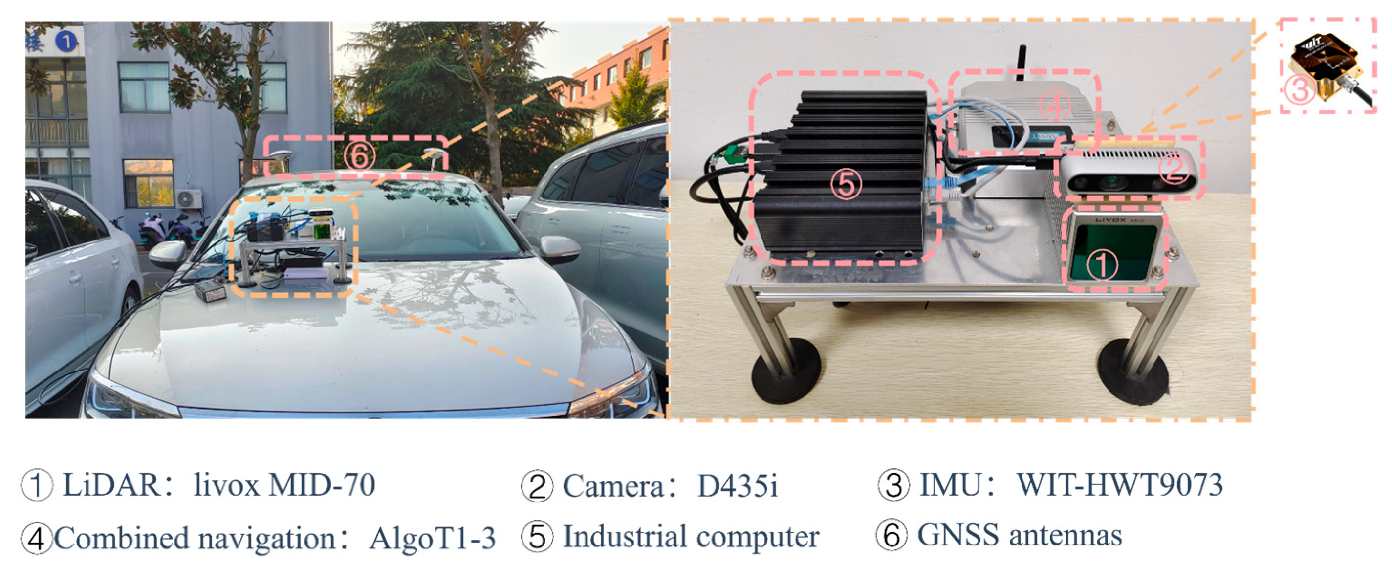
Experiments are conducted using measured data from four scenes. The independently constructed multi-sensor integrated data collection device, as shown in Figure 5, is employed to collect point cloud data using the LIVOX MID70 (Livox Technology Co., Ltd., Shenzhen, China. approximately 850 US dollars), IMU data using low-cost WIT-HWT9073 (WitMotion Shenzhen Co., Ltd., Shenzhen, China. approximately 280 US dollars) with a static zero drift of ±0.5~1°/s when placed horizontally. Images come from D435i (Intel Corporation, Santa Clara, USA. approximately 380 US dollars), and RTK outcome from the AlgoT1 (Shanghai Algebra Rhythm Technology Co., Ltd., Shanghai, China.) with a frequency of 10 Hz (approximately 1150 US dollars). The whole equipment cost less than 2800 dollars. Time reference for each sensor is unified by ROS (Robot Operation System) without time synchronization devices; extrinsic calibration was conducted beforehand.

Figure 5. Overview of sensor configuration on the hardware platform.

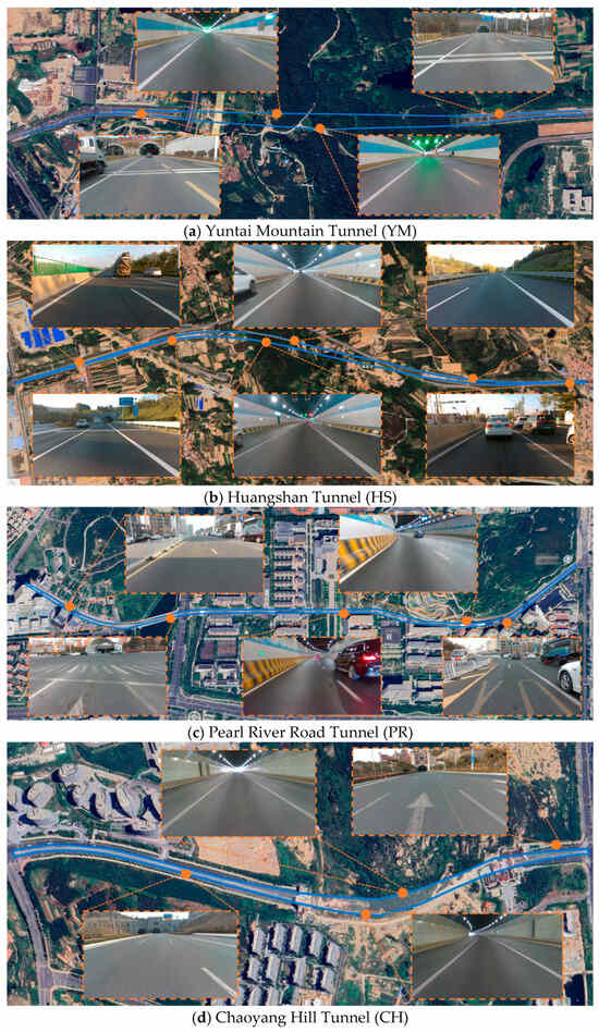
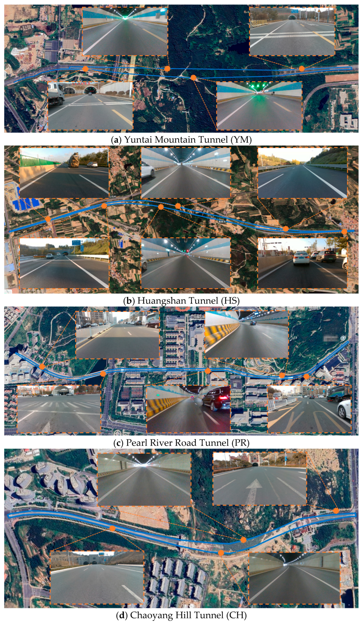
Four datasets were collected in different tunnel environments as shown in Table 1. The first dataset, YM, was acquired in the Yuntai Mountain Tunnel (Figure 6a), an open roadway tunnel equipped with high/low-voltage power systems, fire protection systems, and bilateral ventilation systems. The second one, HS, was gathered in the Huangshan Tunnel (Figure 6b), a bidirectional, double-hole tunnel with four lanes per direction and complete infrastructure. The third dataset, PR, was collected in the Pearl River Road Tunnel (Figure 6c), a two-way, four-lane tunnel extending underground with a significant elevation difference relative to the ground surface. The final dataset, CH, was obtained in the Chaoyang Hill Tunnel (Figure 6d), a six-lane structure. The data collection process involved driving through the tunnel from an open area, turning around, returning via the opposite lane, repeating the process within the same tunnel.

Table 1. Parameters of four tunnel data collection sequences.

Dataset	Tunnel Length (m)	Total Length (m)	Duration (s)
Yuntai Mountain Tunnel	1076	7399	705
Huangshan Tunnel	1467	10,778	1060
Pearl River Road Tunnel	998	7562	1075
Chaoyang Hill Tunnel	515	5480	629

Figure 6. Bird view of the dataset collection scene. (a–d) illustrate the data acquisition scenarios for the Yuntai Mountain Tunnel (YM), Huangshan Tunnel (HS), the Pearl River Road Tunnel (PR), and the Chaoyang Hill Tunnel (CH), respectively.

4.1. Performance Comparison on Loop Closing Module and RTK Processing and Quality Control Module

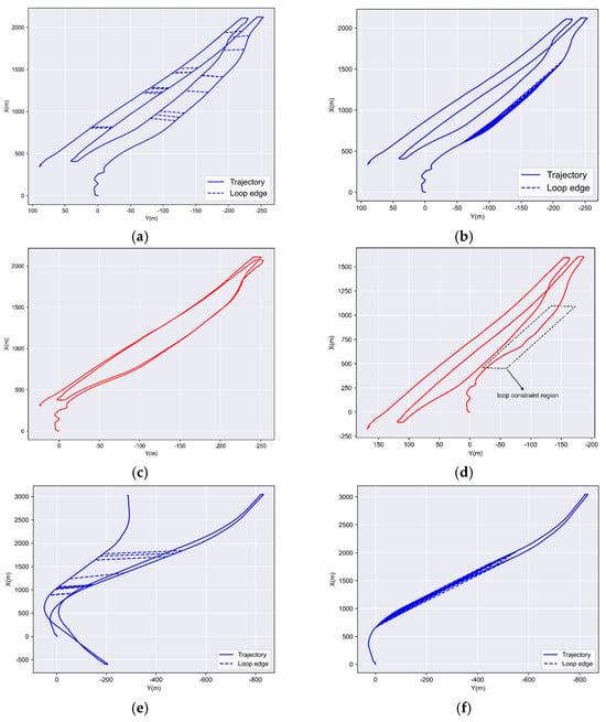
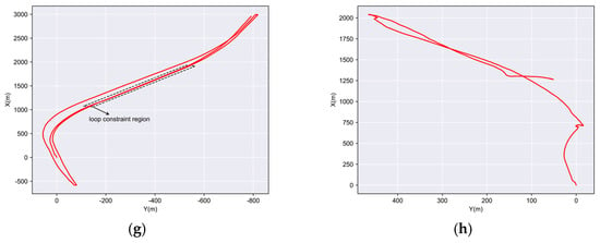
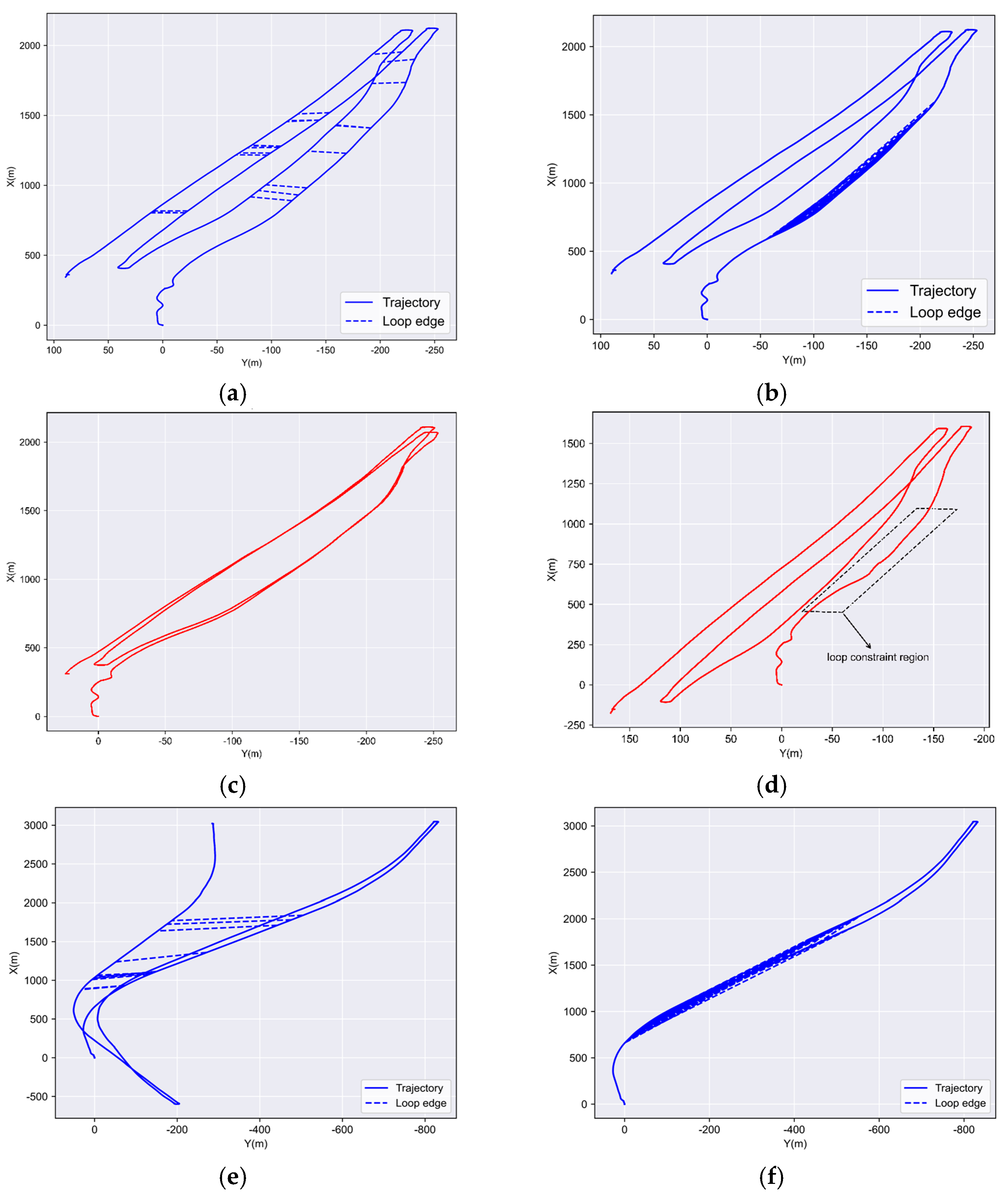
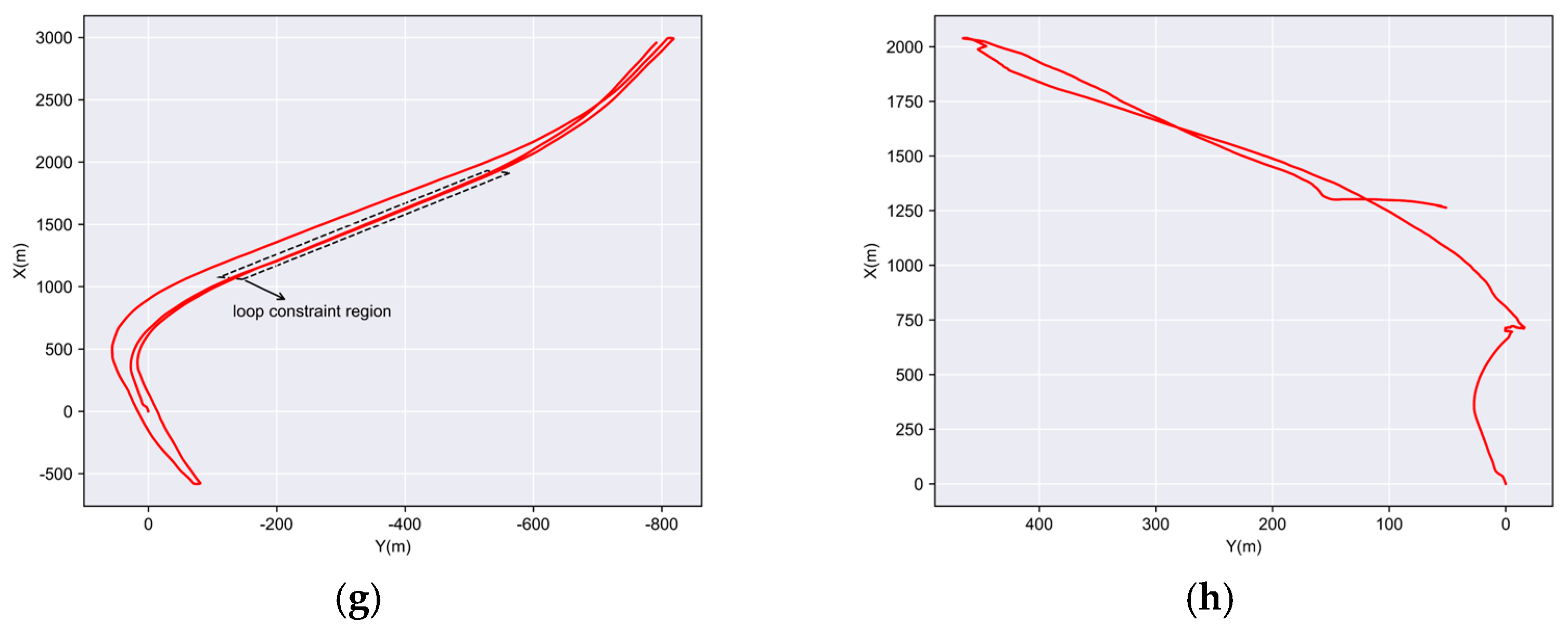
We used the YM and HS datasets to validate the proposed loop detection method due to their complete tunnel infrastructure. A comparison was conducted between the proposed descriptor and Scan Context. The blue trajectories in Figure 7a,e represented the LIO trajectory without RTK and loop constraints, where the blue line segments connecting the trajectories indicate detected loop closures. Figure 7c,g showed the trajectories after loop constraints are added, demonstrating that repeated data acquisition is constrained to align with the same trajectory. We compared our method with Scan Context in Figure 7b,f, which revealed a large number of false loop detections in the tunnel sections when using Scan Context. These erroneous loop constraints significantly degrade the consistency of pose estimation, as shown in Figure 7d,h. This was due to the single geometry in the tunnel and limited field of view of the solid-state LiDAR. The proposed loop-closure detection and matching method effectively mitigates accumulated drift, ensuring global trajectory consistency.

Figure 7. The proposed loop closing method vs. Scan Context on the YT and HS datasets. (a,e): The LIO trajectory and the loop edges identified by SLD based loop detection method. (b,f): The LIO trajectory and the loop edges detected by the Scan Context method. (c,g): Trajectory after adding the proposed loop constraints from SLD to the LIO. (d,h): Trajectory after adding Scan Context loop constraints to the LIO.

As shown in Table 2, the descriptor generation time of the proposed method (0.0354 ms) is comparable to that of Scan Context (0.0416 ms). In the matching stage, however, the proposed method reduces the matching time to 0.0045 ms, achieving nearly two orders of magnitude speed improvement compared with Scan Context (0.3739 ms). The efficiency gain mainly arises because, unlike Scan Context which performs dense encoding on the raw point cloud of each frame, the proposed method constructs descriptors based on sparse semantic points within a local range, thereby effectively reducing data redundancy and accelerating the retrieval process.

Table 2. Runtime analysis of descriptor generation and matching modules.

Method	Generation Time (ms)	Matching Time (ms)
Scan Context	0.0416	0.3739
Ours	0.0354	0.0045

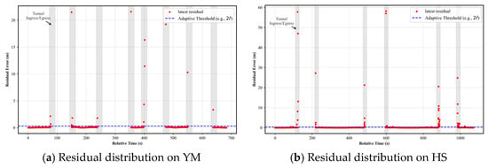
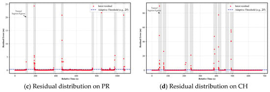
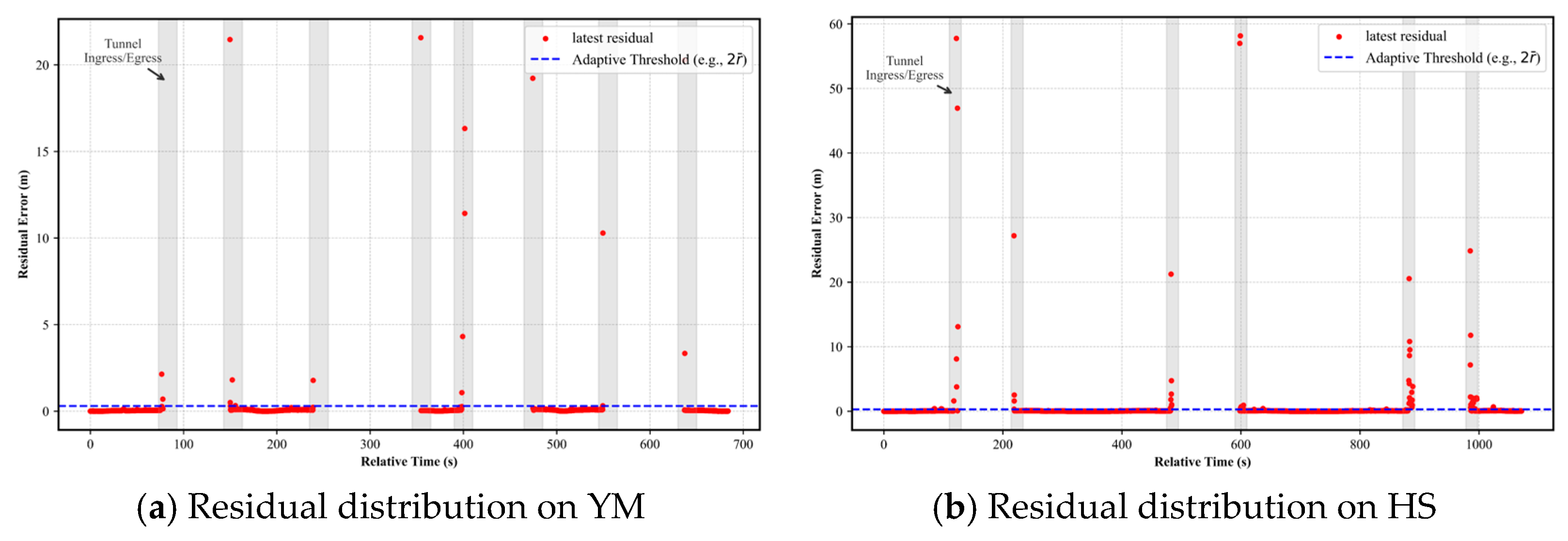
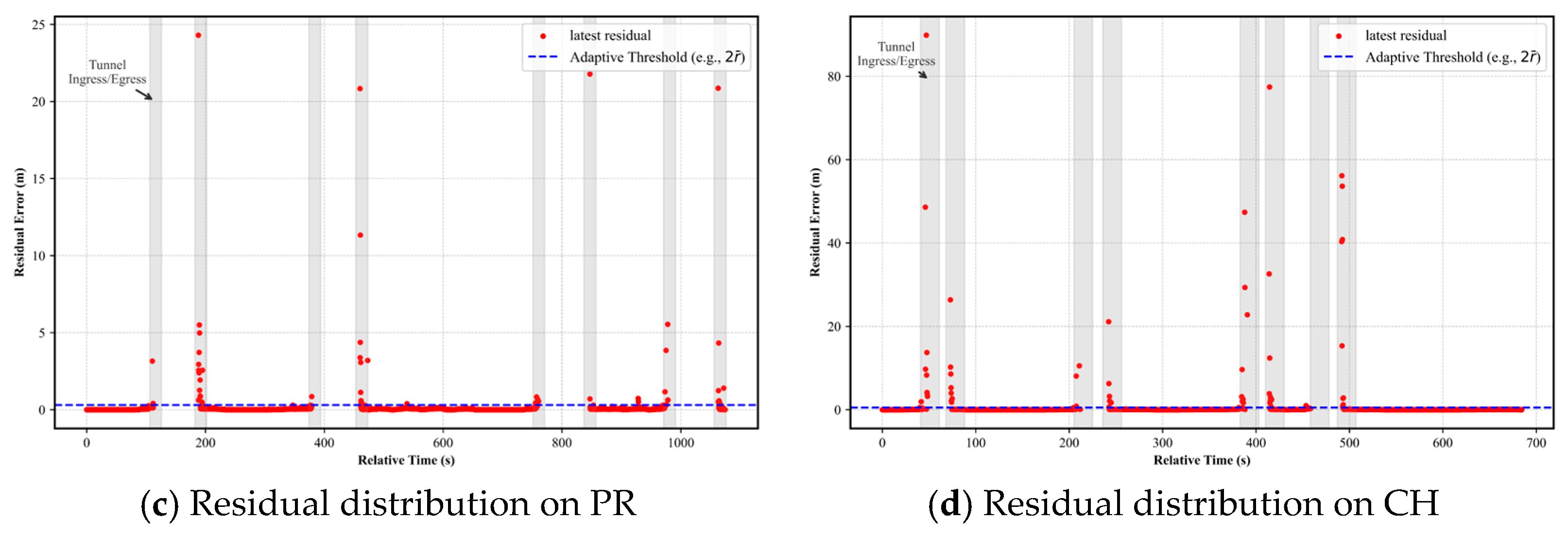
To validate the effectiveness of the proposed two-stage RTK quality control mechanism, we analyzed the statistical distribution of residuals computed using Algorithm 2. Figure 8 illustrates the temporal evolution of these residuals across four tunnel sequences collected during the experiments. As shown in the figure, the statistical results indicate that when driving in open environments, the residuals exhibit an extremely low mean and a stable distribution. In contrast, during tunnel ingress and egress, the residuals increase sharply due to the presence of abnormal RTK measurements. This distinct distribution pattern validates the effectiveness of the adopted outlier rejection strategy. Moreover, the clear separation between the two regimes demonstrates that the system is highly robust to the choice of threshold.

Figure 8. Distribution of B-spline fitting residuals calculated via Algorithm 2 and evaluation of the adaptive thresholding strategy. (a–d) correspond to four distinct experimental sequences. The blue dots denote the residuals ($r_i=‖p_i-{\tilde{p}}_i‖$) derived from Algorithm 2. The gray shaded zones indicate tunnel ingress and egress phases; the red dashed line denotes the adaptive threshold.

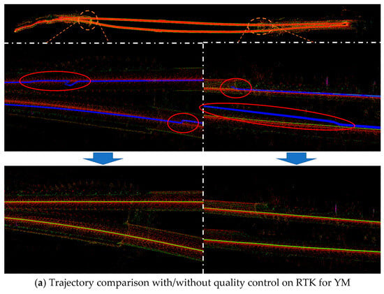
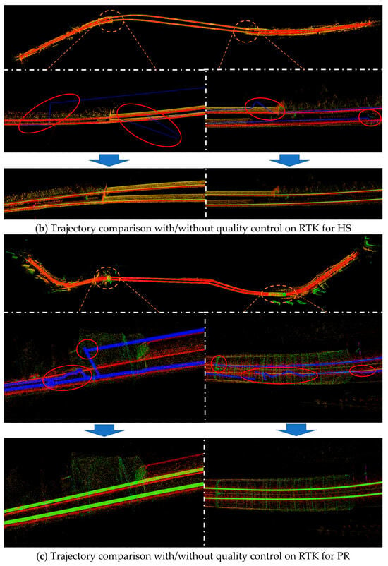
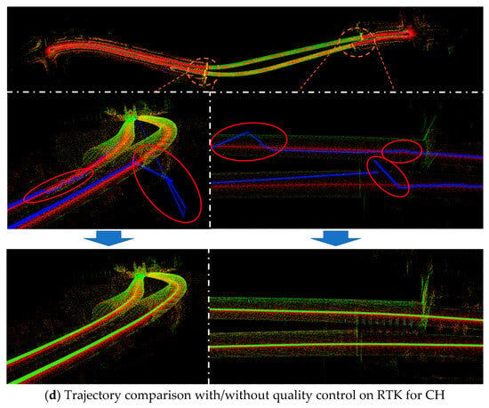
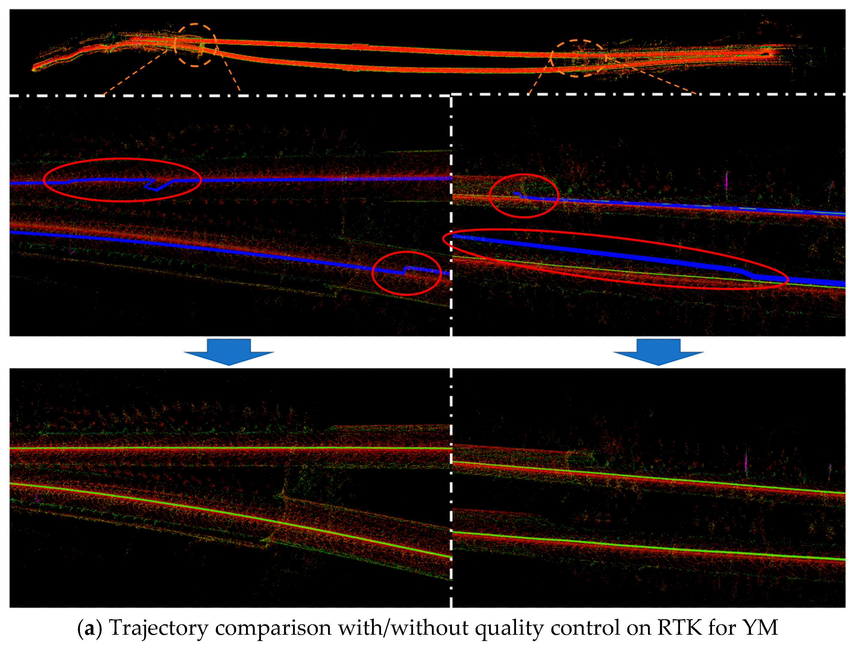
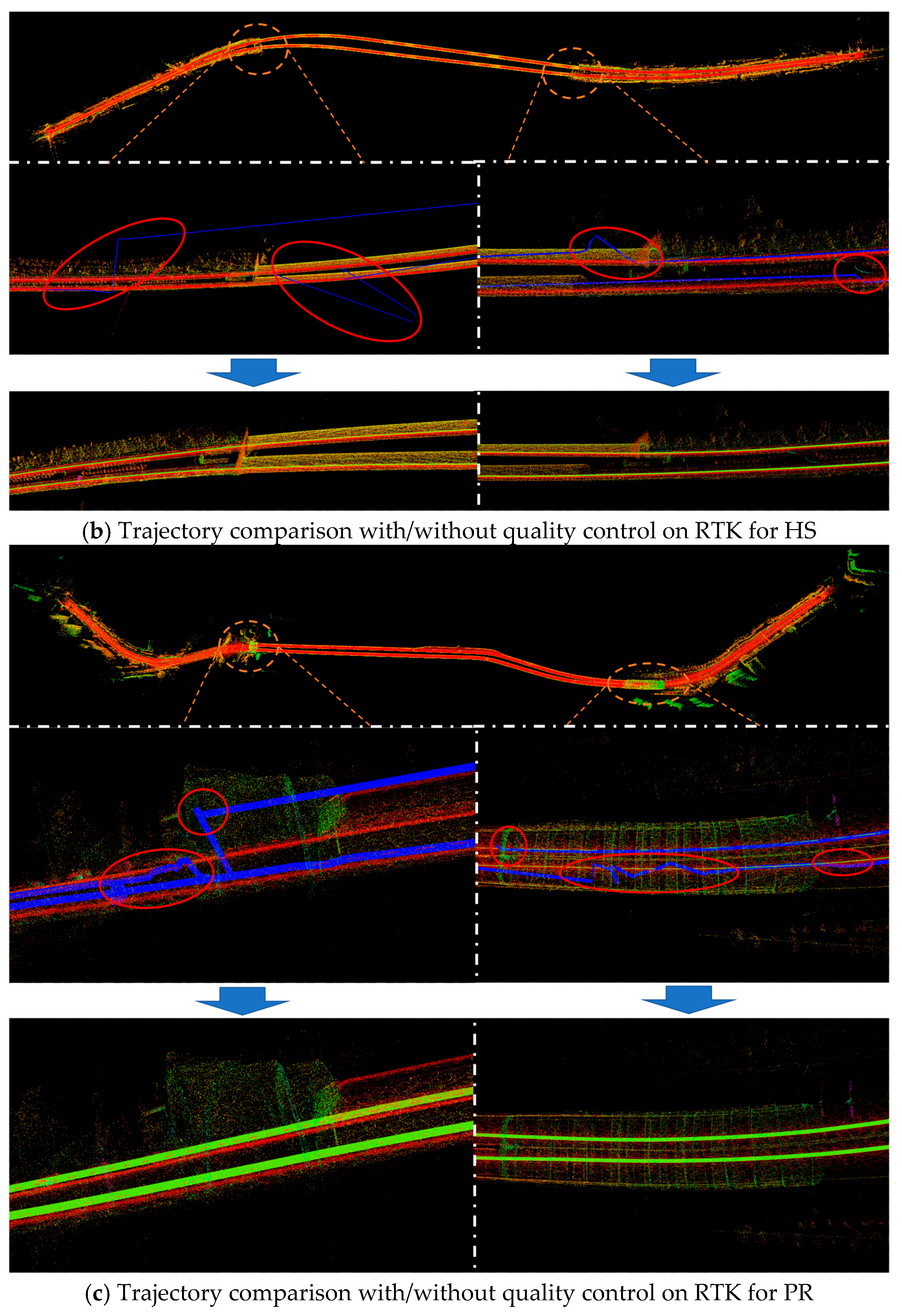
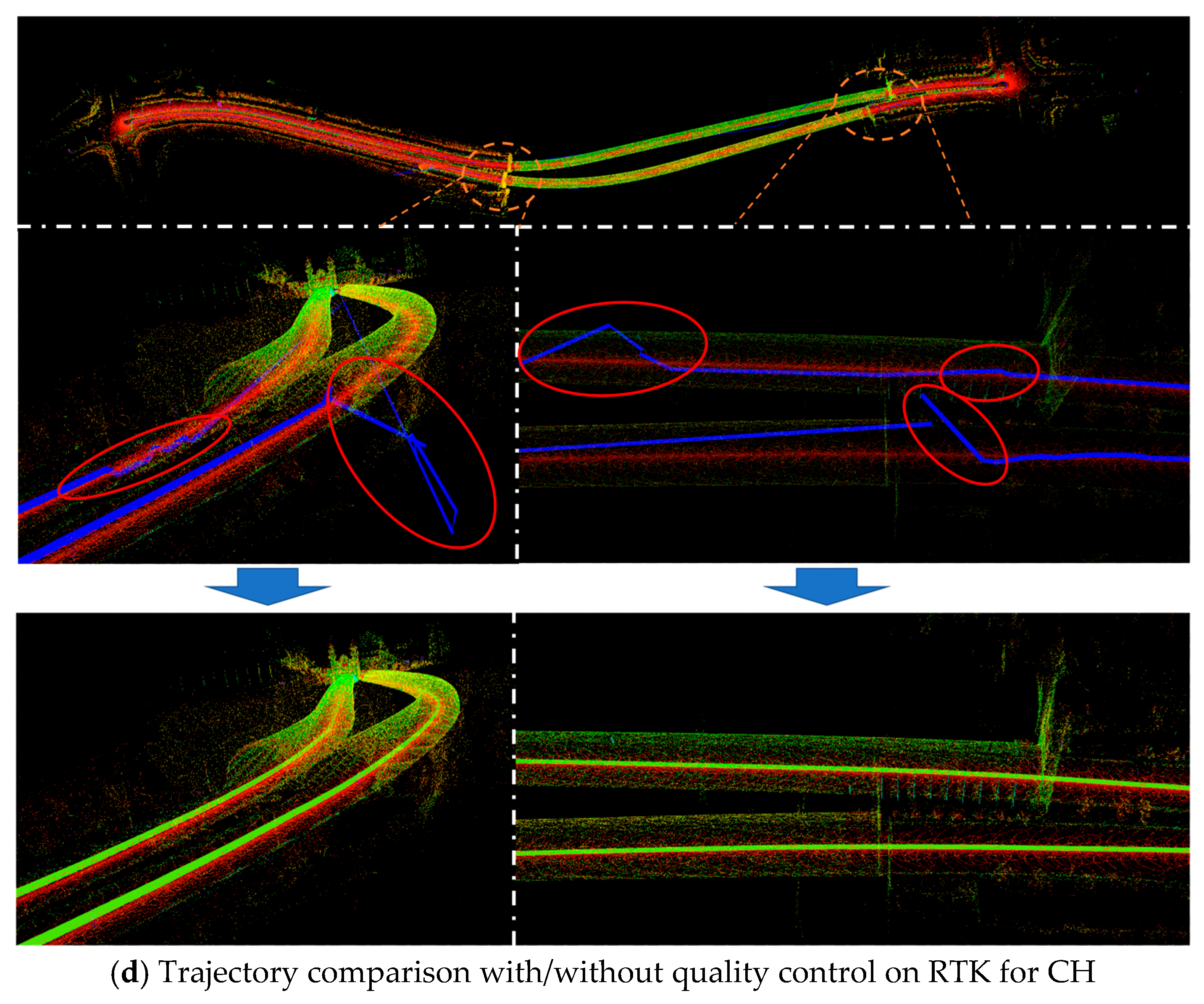
Figure 9a–d illustrated the anomalies in RTK position results when entering and exiting the tunnels for the four datasets, as well as the estimated trajectories of the pose with quality control. The blue line represented the RTK positioning trajectory, while the red circle highlighted the trajectory during RTK positioning anomalies. The proposed quality control strategy was designed to prevent larger erroneous position results from being introduced into the overall localization system, thereby significantly reducing drift and maintaining the consistency of pose estimation. Following the blue arrow, the green trajectory in the lower part of Figure 9a–d is notably smooth and consistent with the strategy of quality control.

Figure 9. RTK position anomalies during entry and exit tunnel scenarios and trajectories following quality control implementation. (a–d) are the Yuntai Mountain Tunnel scene, Huangshan Tunnel scene, Pearl River Road Tunnel scene and Chaoyang Hill Tunnel scene, respectively. Red circles indicate GNSS outliers near tunnel entrances and exits. The blue line denotes the raw GNSS positioning trajectory, while the green line denotes the smoothed trajectory after quality control generated by the proposed system.

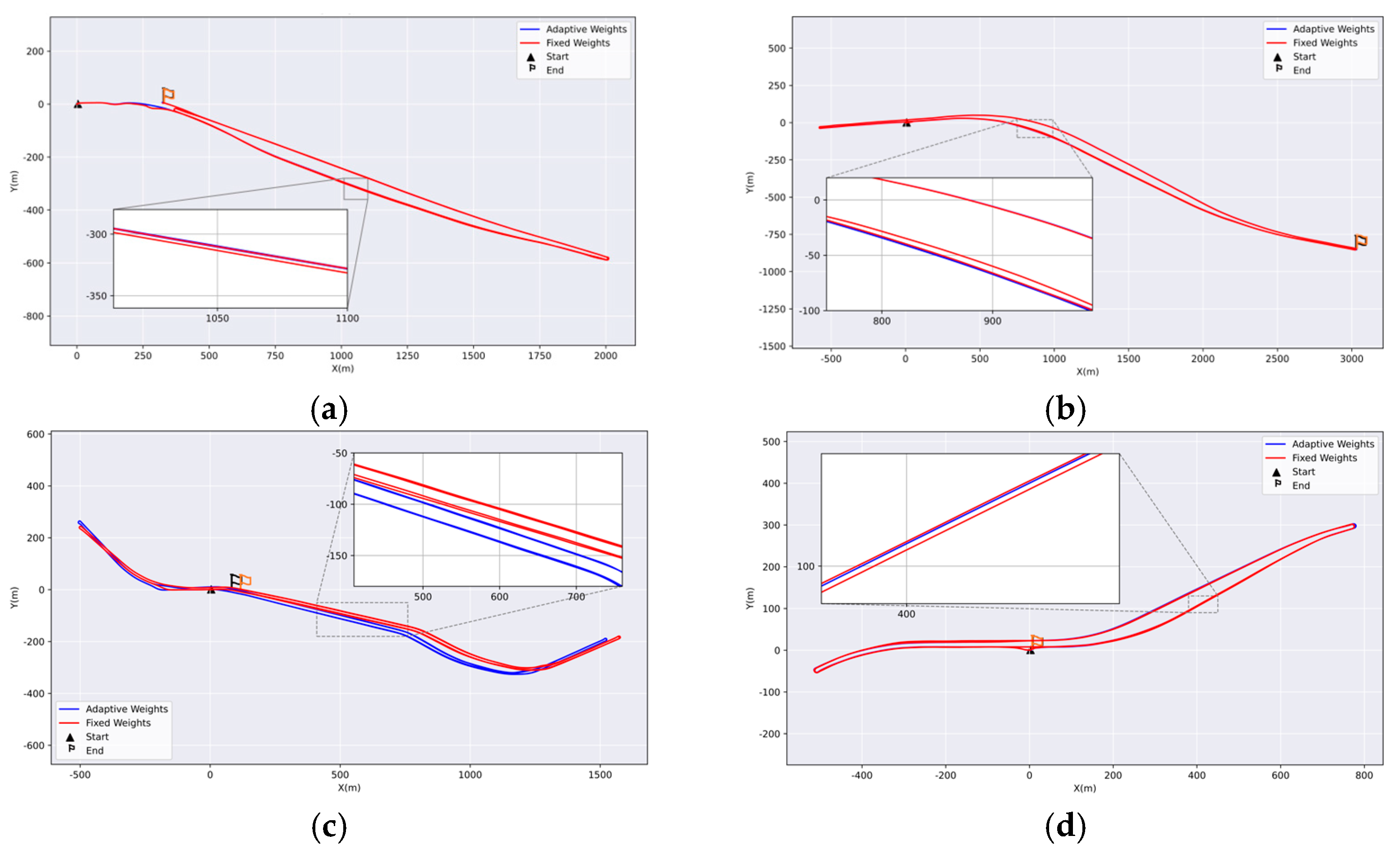
To validate the effectiveness of the proposed adaptive weighting strategy, we conducted comparative experiments using fixed weights. The fixed weight values were empirically selected from within the range determined by the adaptive weighting scheme. As shown in Figure 10, across all four datasets, the red trajectories obtained from repeated runs exhibit significantly larger deviations inside the tunnel than the blue trajectories, resulting in poorer global consistency. This phenomenon mainly arises from the fact that different environmental regions provide varying levels of constraint for pose estimation. Inside tunnels, the corridor-like structure causes geometric information to degenerate along certain directions, reducing observation reliability. In contrast, outside the tunnel or in structurally richer areas, the environment offers stronger geometric constraints, leading to more stable pose estimation. Applying uniform weights to residuals in all directions can therefore introduce improper constraints in degenerate directions and degrade overall optimization consistency. By contrast, the proposed adaptive weighting strategy dynamically adjusts the constraint strength according to the scene and observation conditions, reducing weights in degenerate directions while strengthening them in reliable ones, thereby maintaining more stable global trajectory consistency during transitions across different environments.

Figure 10. Comparison of weighting strategies on four datasets. (a) Trajectory with different weighting strategies on YM; (b) trajectory with different weighting strategies on HS; (c) trajectory with different weighting strategies on PR; (d) trajectory with different weighting strategies on CH.

4.2. Overall Performance Comparison with SOTA Methods

The summary of test results from the current state-of-the-art LIO and Tunnel-SLAM was shown in Table 3. All baseline methods were tested using the official open-source implementations with default parameters as recommended by the authors. Except for necessary modifications to the input data configuration, no additional parameter tuning was performed. FAST-LIO2 [15] experienced position-estimate drift after exiting the tunnel portal in YM and HS. Adaptive-LIO [47] produced erroneous pose estimations when a large truck passes by in HS. DLIO [48] exhibited drift after encountering dynamic objects in the HS sequence, while in the other three datasets it showed significant drift immediately upon entering the tunnel. Point-LIO [49] exhibited drift during the system initialization stage. IG-LIO [50] exhibited drift both after encountering dynamic objects and upon entering the tunnel. In high-speed driving, motion blur and rapid FOV changes degrade FAST-LIVO2’s [51] visual feature tracking, causing rapid trajectory drift at the very beginning of the data sequence. Only Tunnel-SLAM successfully processed all datasets.

Table 3. Performance comparison between Tunnel-SLAM and other SOTA methods.

	FAST-LIO2	Adaptive-LIO	DLIO	FAST-LIVO2	Point-LIO	IG-LIO	Ours
YM	●	✓	▲	✘	✘	✘	✓
HS	●	◆	◆	✘	✘	◆	✓
PR	✓	✓	▲	✘	✘	◆	✓
CH	✓	✓	▲	✘	✘	▲	✓

✓ denotes that the system successfully run the dataset. ✘ denotes that the system failure at the start of the sequence. ▲ denotes that the system failure in the tunnel. ◆ denotes that the system failure in the presence of dynamic objects. ● denotes that the system failure after exiting the tunnel portal.

To evaluate the effectiveness and applicability of the proposed framework, we conducted a comparison of position estimation across four datasets. Moving cars and pedestrians also influenced the system, reflecting the real-world conditions of the road tunnel environment. Consequently, the experiments validated the effectiveness and robustness of the proposed integrated system.

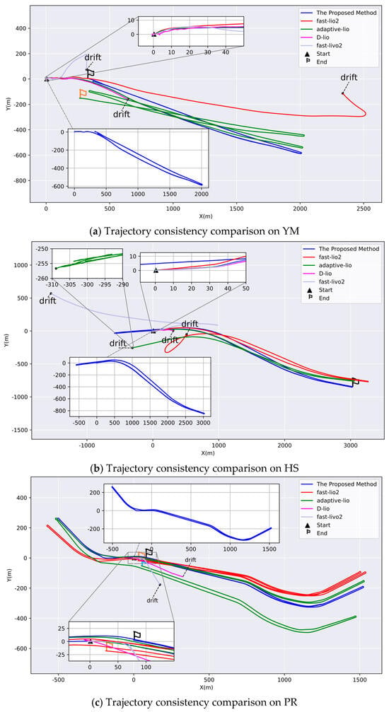
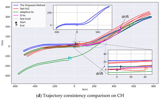
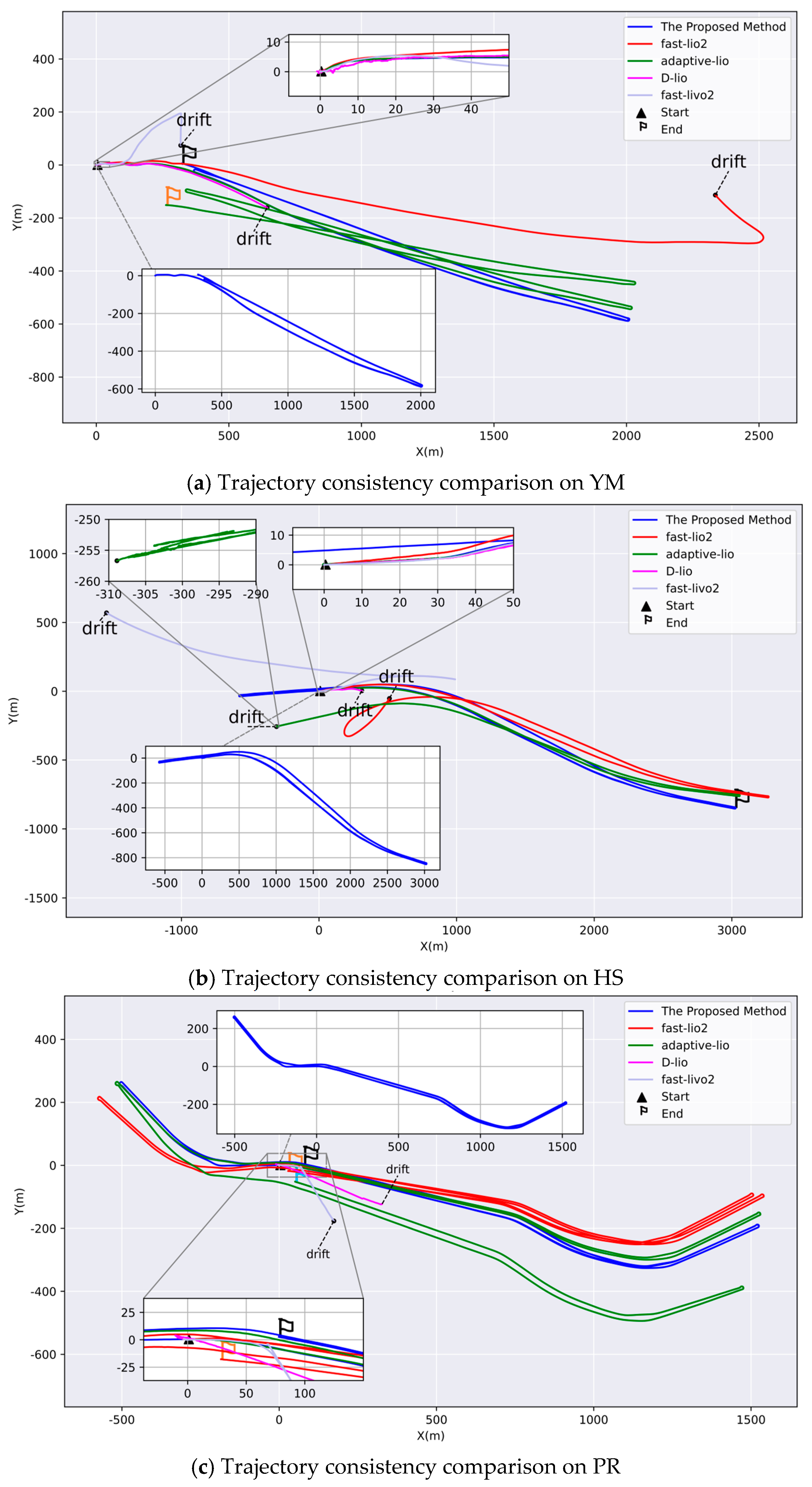
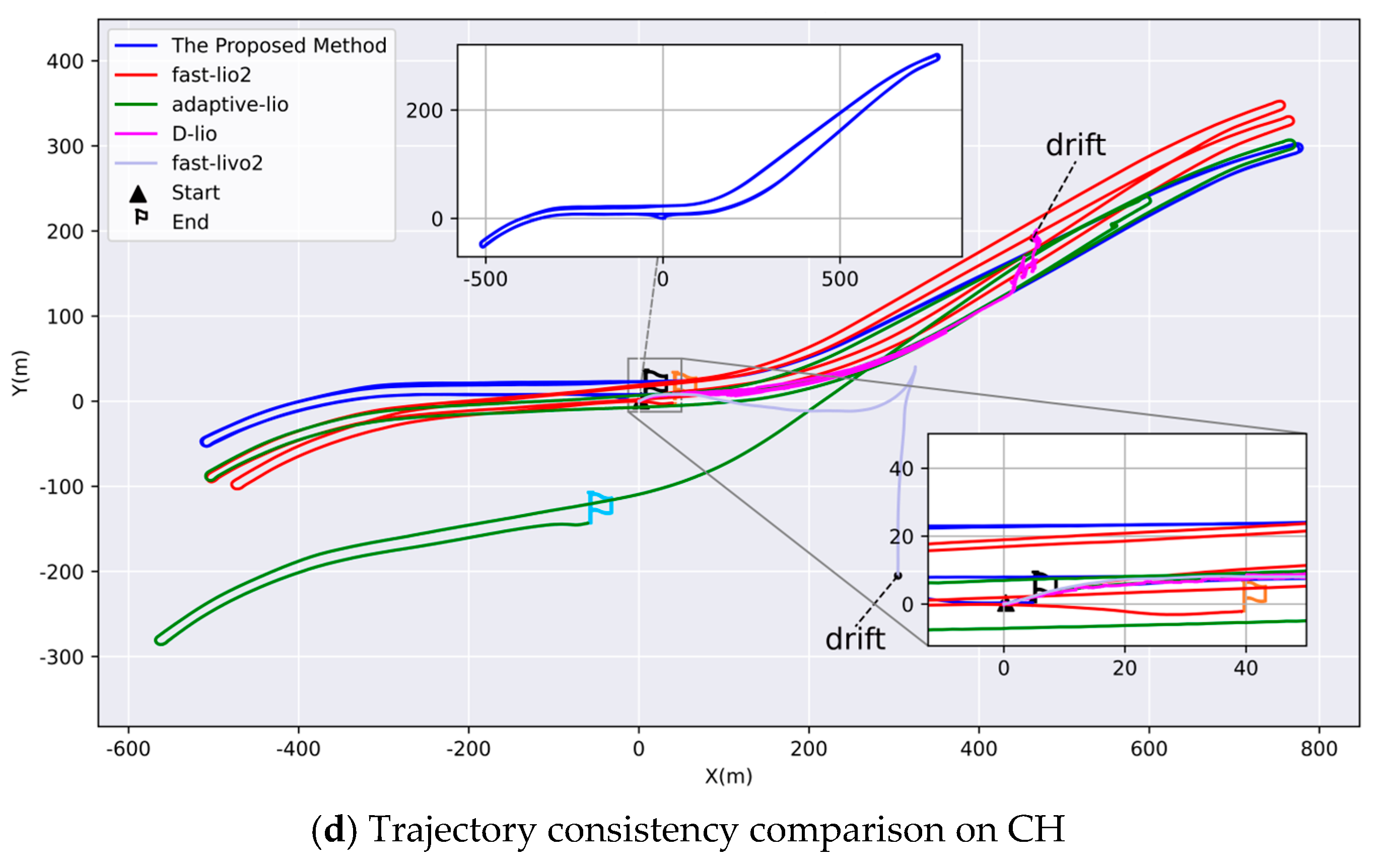
Figure 11 presents a comparative analysis of the results obtained using different methods on four tunnel datasets. From the zoomed-in view, the trajectory of the D-LIO slightly shifted at the beginning. When the vehicle traveled inside the tunnel, the single geometry of the tunnel caused errors in point cloud registration, leading to the trajectory stopping, backing up, and eventually experiencing significant drift. FAST-LIO2 successfully processed the PR and CH datasets in their entirety. However, vehicle motion and accumulated drift over time resulted in significant divergence in trajectory estimates for the same segment. In the YM and HS dataset, a sudden reduction in the number of LiDAR points upon exiting the tunnel decreased the number of residual constraint equations, leading to substantial drift after extended operation. Adaptive-LIO was able to process all datasets except the HS, where pose estimation errors occurred due to the persistent influence of large trucks in adjacent lanes. Additionally, the estimated trajectory exhibited significant drift due to cumulative error effects. FAST-LIVO2 exhibits limitations when operating in highly dynamic vehicular environments. Aggressive platform motion weakens the tracking capability of the visual subsystem, leading to feature association failures or mismatches. The degradation of visual constraints undermines the stability of the entire system, thereby causing rapid localization drift. In contrast, Tunnel-SLAM successfully processed the entire dataset and maintained good global consistency in pose estimation. which are the results from the combined effects of all proposed modules. The loop-closure module can identify accurate loop candidates and add loop constraints in FGO. The RTK processing module can accept or reject RTK measurements, and FGO assigns appropriate measurements and weights at the right time in challenging tunnel scenarios. All these modules contribute to minimizing net drift in the trajectories and ensuring a consistent mapping process.

Figure 11. Comparison of trajectories of different methods in four datasets: (a) Yuntai Mountain Tunnel; (b) Huangshan Tunnel; (c) Pearl River Road Tunnel; (d) Chaoyang Hill.

Table 4 shows the distance between the start point and the end point for each trajectory, which represents the accumulated drift. It is clear that Tunnel-SLAM consistently achieves the lowest drift. The competing algorithms frequently fail or yield large errors. For example, the other four methods fail in Huangshan Tunnel, but our method drifts 1.440 m. In the scenario of Yuntai Mountain, FAST-LIO2, FAST-LIVO2, and DLIO fail. Adaptive-LIO exhibits a drift of 167.898 m, and our method drifts only 1.956 m.

Table 4. Drift comparison of different algorithms in tunnel scenarios (unit: m).

Datasets	FAST-LIO2	Adaptive-LIO	DLIO	FAST-LIVO2	Ours
YM	Fail	167.898	Fail	Fail	1.956
HS	Fail	Fail	Fail	Fail	1.440
PR	53.398	60.917	Fail	Fail	1.468
CH	34.651	157.714	Fail	Fail	1.377

4.3. Ablation Experiment

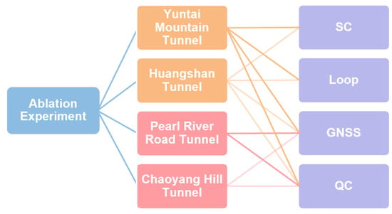
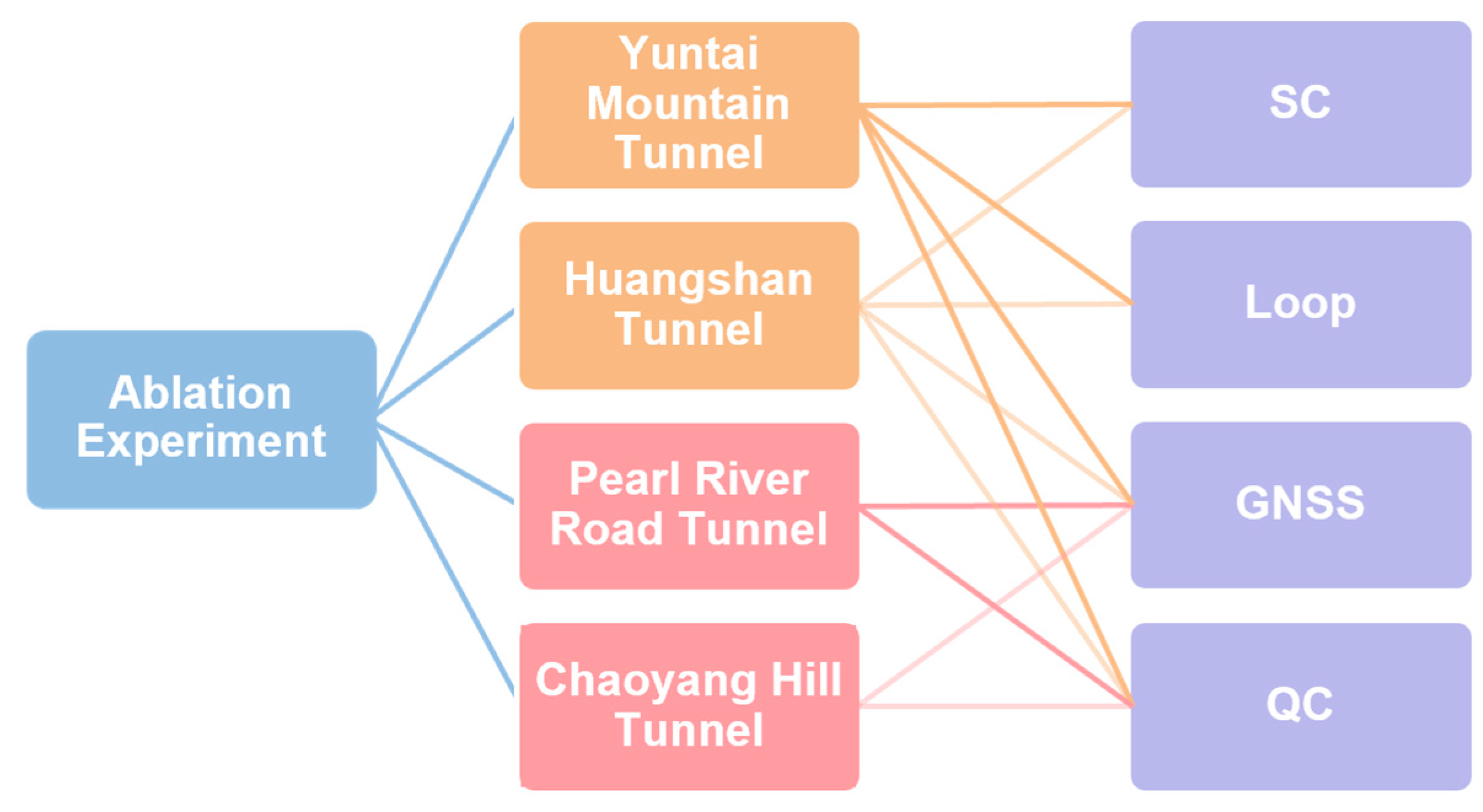
To validate the proposed semantically assisted loop-closure detection module and quality-control (QC) module, we conducted a series of ablation experiments by deactivating the respective modules. The experimental results on four datasets used for the ablation study are shown in Figure 12. It is worth noting that PR and CH datasets are not used for loop-closure detection, as they are small to medium-sized tunnels with limited tunnel facilities, therefore there no SLDs can be generated for them.

Figure 12. Component modules for ablation experiment.

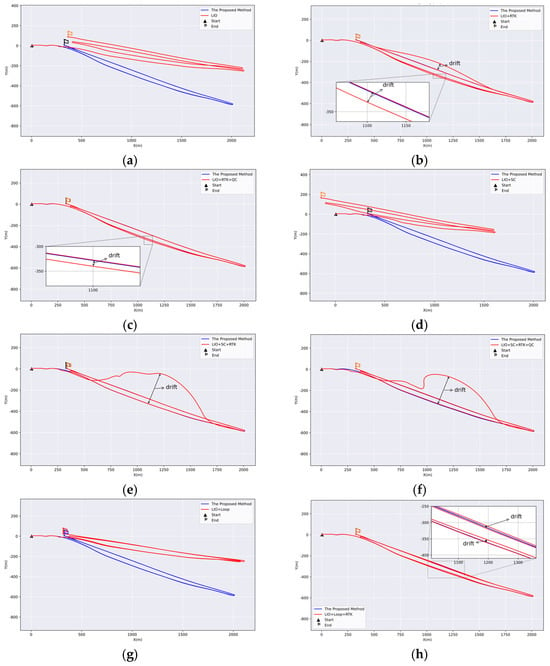
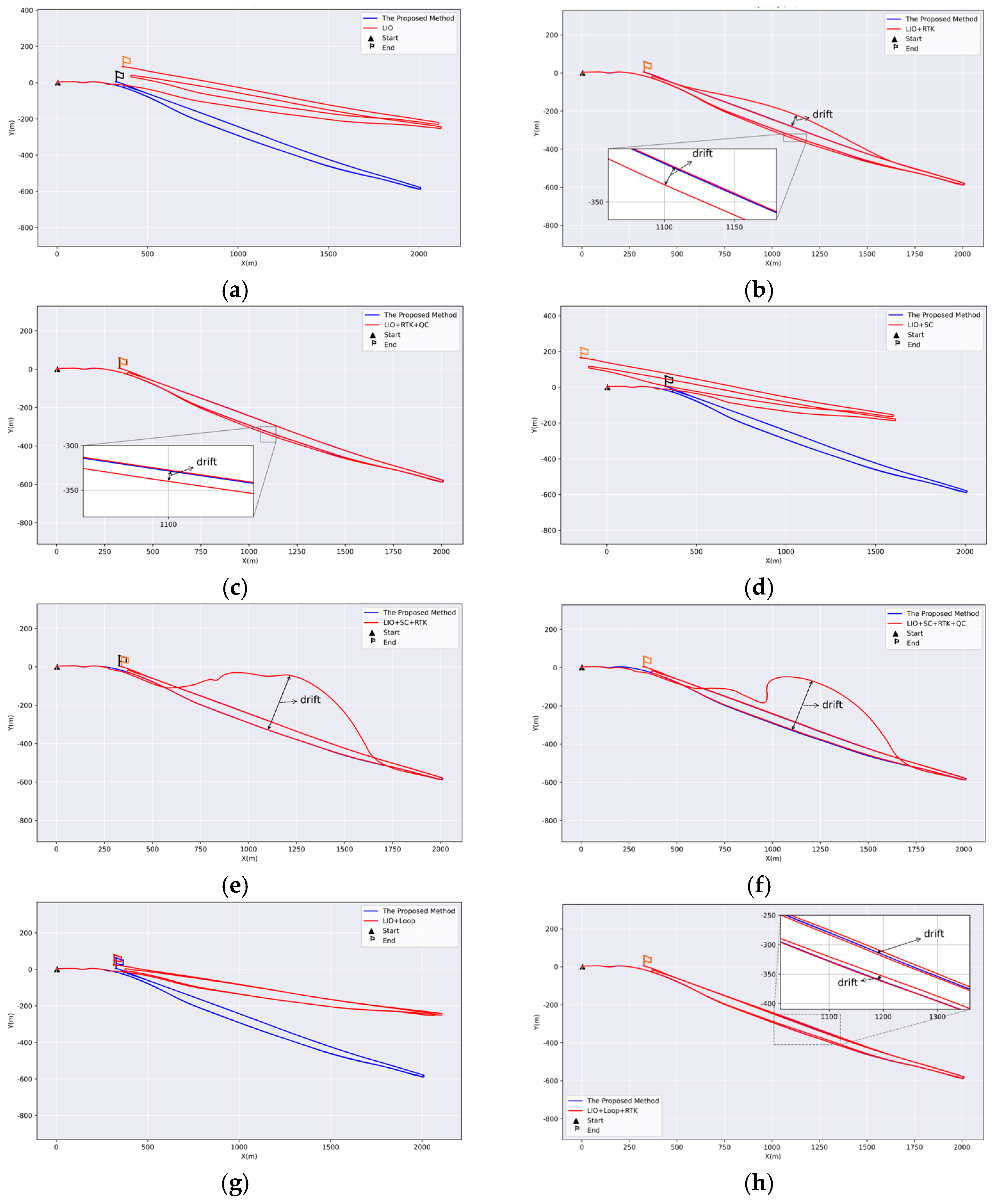
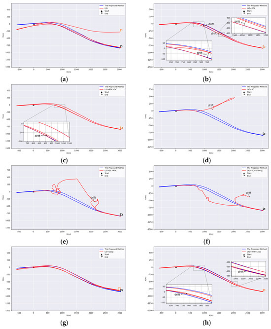
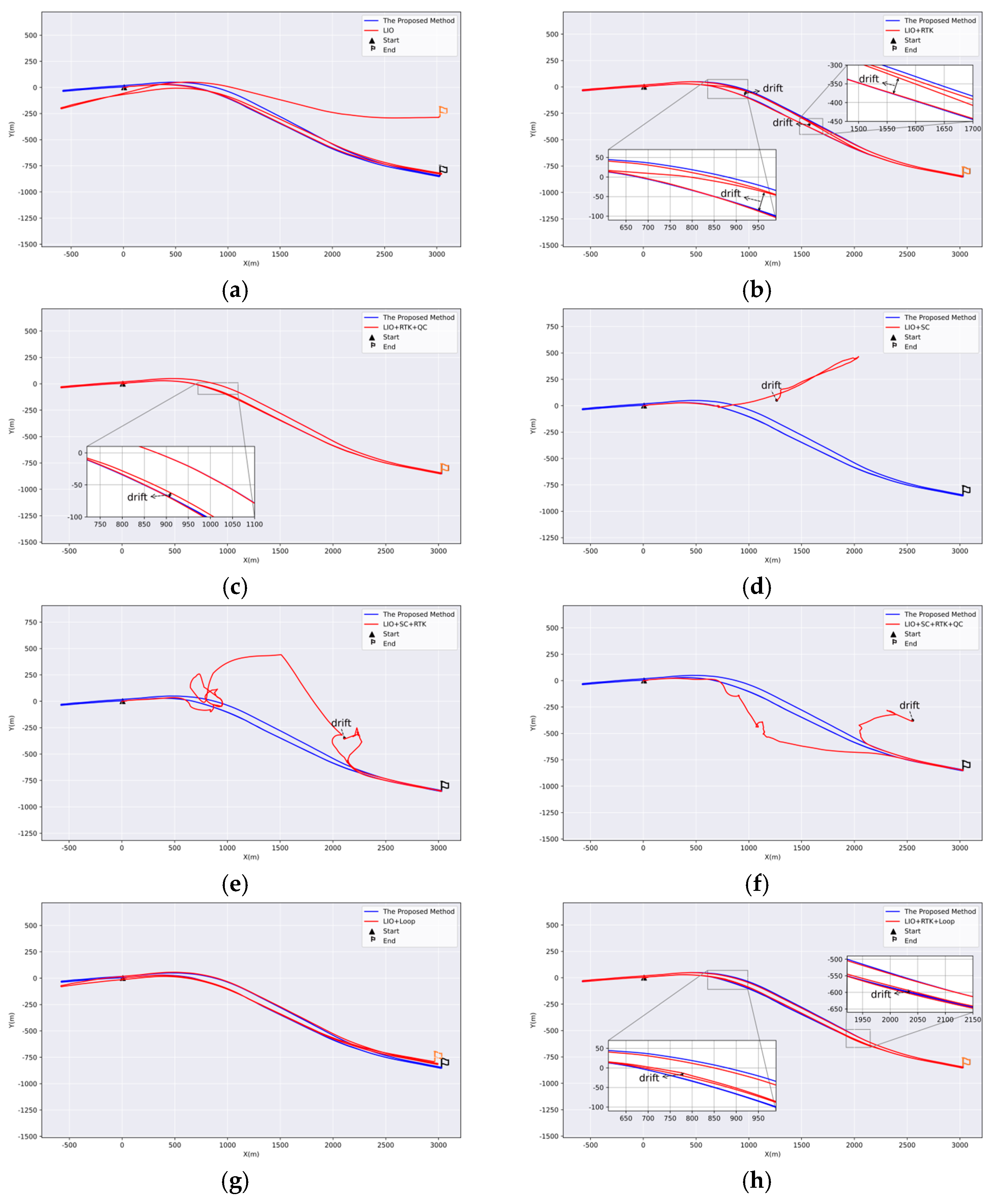
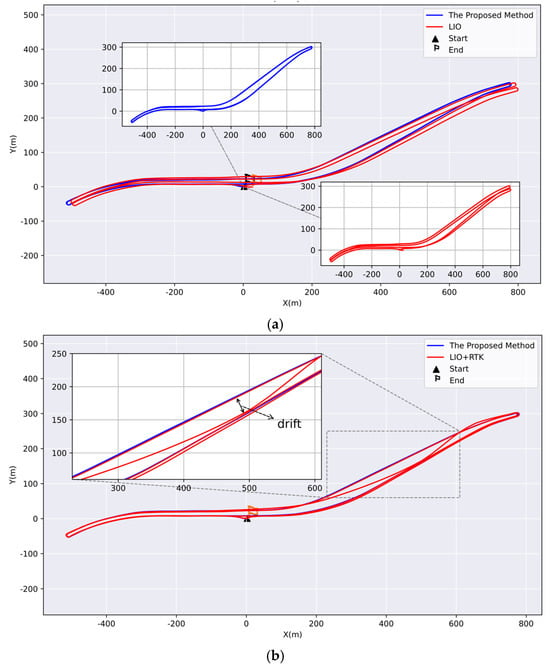
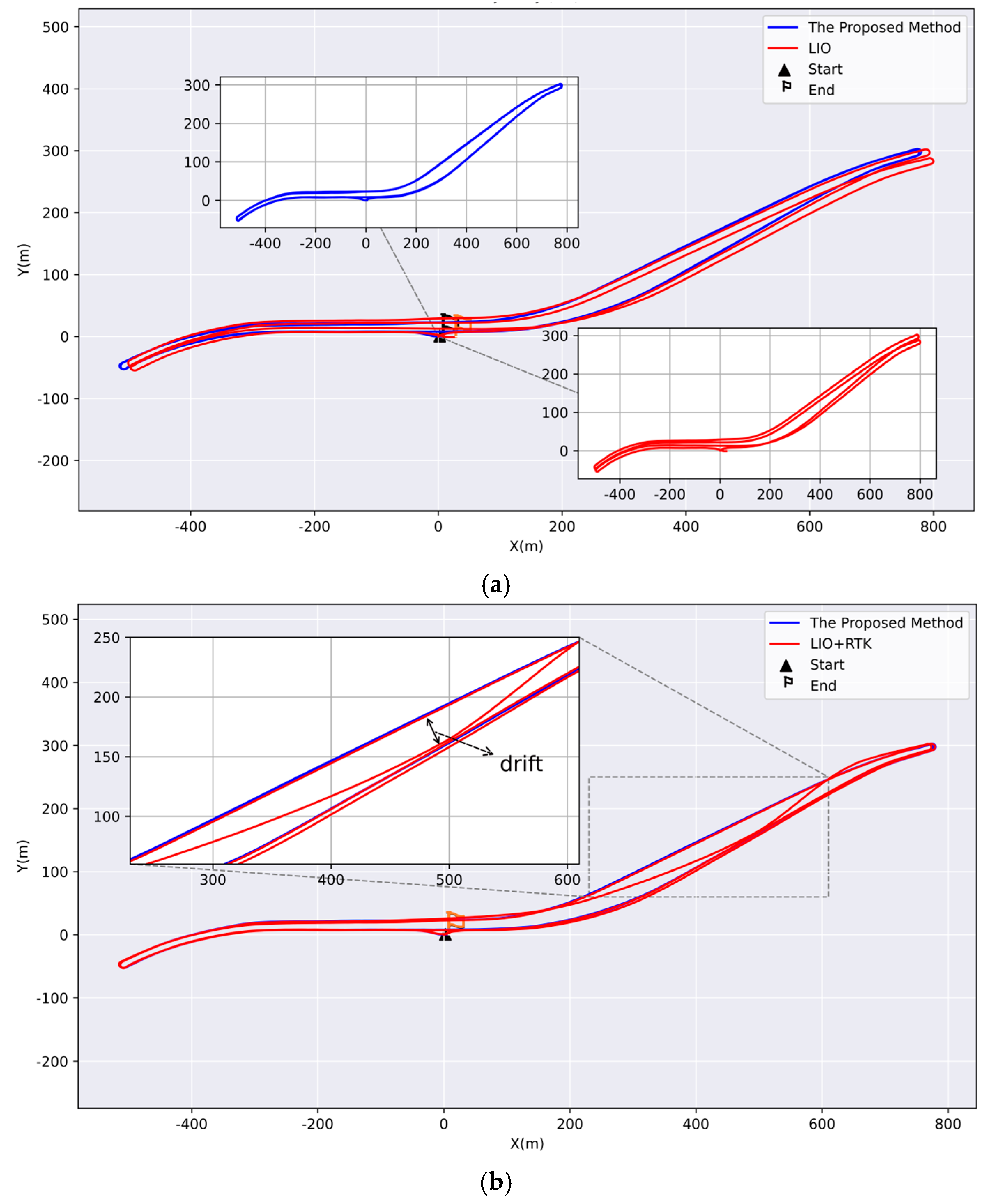
YM Dataset and HS Dataset. Ablation experiments were performed on these two datasets to evaluate four modules: loop closure, RTK, quality control (QC), and Scan Context (SC). When comparing Tunnel-SLAM with pure LIO, it was evident that pure LIO caused a global trajectory shift due to the absence of RTK, which can provide a global coordinate reference. In addition, trajectories corresponding to the same routes were also misaligned, as shown in Figure 13a and Figure 14a. With the assistance of RTK, as illustrated in Figure 13b and Figure 14b, the drift of the overall trajectory was suppressed, but the trajectories of the same paths exhibited a large offset due to RTK anomalies and the absence of loop-closure constraints. After incorporating the QC module, RTK outliers were rejected, and the trajectory drift of the same path was further suppressed to some extent. However, due to the lack of loop constraints, the trajectory was still globally inconsistent, as shown in Figure 13c and Figure 14c. As shown in Figure 13d and Figure 14d, incorporating SC-based loop detection into the pure LIO results in system drift or even collapse when erroneous loop-closure constraints occur, thereby leading to a substantial degradation in overall consistency. As shown in Figure 13e,f, RTK and RTK with QC were incorporated, respectively; however, both exhibited substantial drift in the tunnel region, primarily due to erroneous loop-closure detection. In Figure 14e,f, erroneous loop-closure detection in the tunnel region caused substantial trajectory drift, ultimately leading to the collapse of the entire pose estimation system. In Figure 13g and Figure 14g, we integrated the proposed loop detection module into the pure LIO. The results showed that the trajectories of the same path exhibited better consistency. However, the overall trajectory still exhibited significant drift due to the absence of RTK. Figure 13h and Figure 14h, on the other hand, show the trajectory of the same route with the RTK and loop-detection module active, but with the QC module turned off. The trajectory shifted due to RTK anomalies at the entrance and exit of the tunnel. In contrast, Tunnel-SLAM algorithm demonstrates a globally consistent trajectory with exceptionally low drift.

Figure 13. Shows the results of the ablation experiments on the Yuntai Mountain Tunnel dataset, where each subplot compares the trajectories of TunnelSLAM with those of the other eight methods: (a) LIO; (b) LIO + RTK; (c) LIO + RTK + QC; (d) LIO + SC; (e) LIO + SC + RTK; (f) LIO + SC + RTK + QC; (g) LIO + Loop; and (h) LIO + Loop + RTK.

Figure 14. Shows the results of the ablation experiments on the Huangshan Tunnel dataset, where each subplot compares the trajectories of Tunnel −SLAM with those of the other eight methods: (a) LIO; (b) LIO + RTK; (c) LIO + RTK + QC; (d) LIO + SC; (e) LIO + SC + RTK; (f) LIO + SC + RTK + QC; (g) LIO + Loop; and (h) LIO + RTK + Loop.

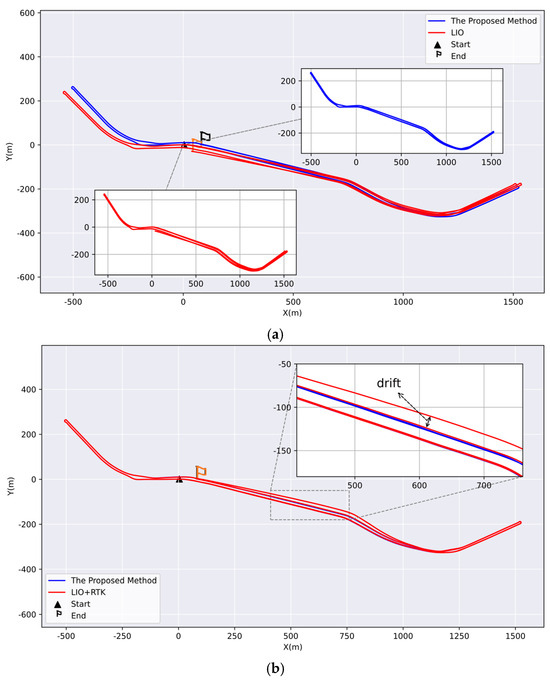
• Pearl River Road dataset. We compared methods with and without the QC module using datasets from Pearl River Road. The red trajectory in Figure 15a represents the result without RTK, and it is evident that the overall path exhibits a noticeable shift. Additionally, trajectory segments along the same route were inconsistent. Figure 15b illustrated that the trajectory of the middle section of the tunnel shifted without QC, with a maximum displacement exceeding 15 m. The trajectory from Tunnel-SLAM maintained a good global consistency.
  

  Figure 15. Validation of RTK module and the QC module in the Pearl River Road dataset. (a) Com-parison of trajectories with and without the RTK Module in LIO. (b) Comparison with and without the QC module integrated into the LIO.
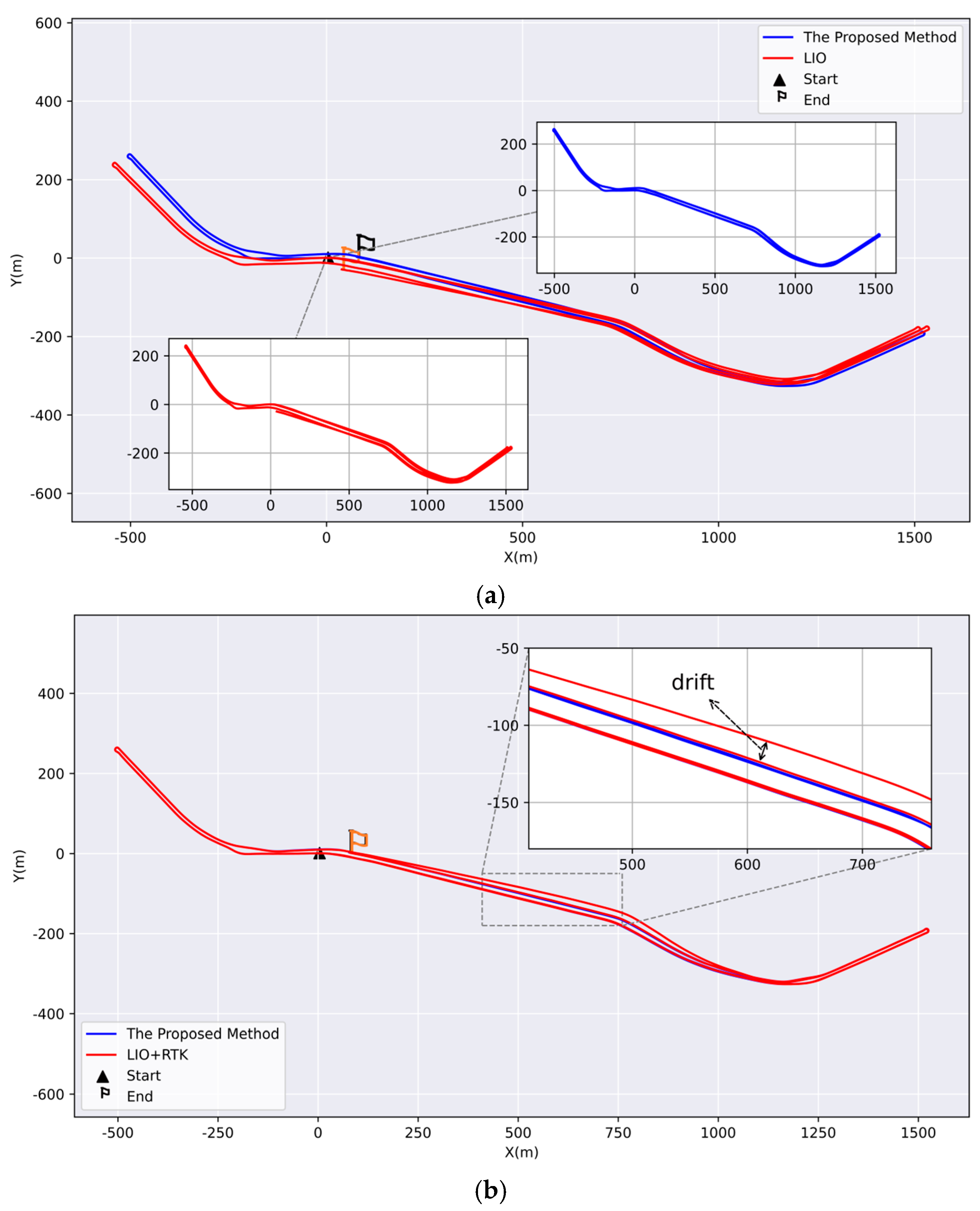
• Chaoyang Hill Tunnel dataset. The same protocol was used for the Pearl River Road dataset. Figure 16a demonstrated that the red trajectory shifted in the region of repeated data acquisition, whereas a globally consistent blue trajectory was obtained in the same region with RTK. The blue and red trajectories correspond to Tunnel-SLAM and the pure LIO method, respectively. Figure 16b depicted the trajectory without the QC module, showing the introduction of outliers and resulting in a red-shifted trajectory. In contrast, the blue trajectory incorporated the RTK and QC modules and maintained global consistency throughout.
  

  Figure 16. Validation of the RTK module and the QC module. (a) Comparison of Trajectories with and without the RTK and QC Module. (b) Comparison of trajectories with and without the QC module.

4.4. Efficiency Evaluation

We conducted an efficiency evaluation to verify the real-time performance of Tunnel-SLAM. Table 5 shows the average runtime breakdown of each Tunnel-SLAM module. Measurement processing dominates the budget at 11.71 ms, followed by graph optimization at around 7.54 ms. Map increment, IESKF correction, and loop-descriptor construction are all sub-millisecond tasks, taking 0.19 ms, 0.83 ms and 0.07 ms respectively. Table 5 demonstrates that Tunnel-SLAM meets real-time requirements for tunnel inspection vehicles. In terms of overall performance, Tunnel-SLAM has a total average execution time of 20.34 ms. Due to the additional computational overhead introduced by modules such as loop closure and factor graph optimization (FGO), this is higher than that of FAST-LIO2 (6.73 ms) and Adaptive-LIO (13.67 ms). However, the corresponding processing frequency of approximately 49 Hz is still higher than the typical LiDAR sampling rate (10–20 Hz). Therefore, Table 5 indicates that Tunnel-SLAM can effectively meet the real-time requirements of tunnel inspection vehicles.

Table 5. Average runtime analysis of tunnel-slam modules and total time comparison with SOTA methods.

	Proc.Meas.	Map Inc.	IESKF	Loop Desc.	Opt.	Tunnel SLAM	FAST_LIO2	Adaptive_LIO
Avg. Time (ms)	11.714	0.186	0.832	0.067	7.537	20.336	6.732	13.668

5. Conclusions

In this paper, we present a robust narrow field-of-view LiDAR-centric RTK-visual-inertial SLAM framework tailored for roadway tunnel inspection using low-cost sensors. To address the limitations of conventional LIO frameworks and geometry-based loop closure methods in degenerate tunnel environments, the proposed system incorporates three key innovations: a semantic-assisted loop detection module that effectively disambiguates repetitive structures where traditional geometric descriptors are prone to perceptual aliasing; a two-stage RTK quality control mechanism that mitigates signal instability during tunnel ingress and egress; and an adaptive factor graph optimization framework that maintains global consistency under varying sensor reliability. Experimental results demonstrate that Tunnel-SLAM achieves low-drift pose estimation and mapping performance comparable to state-of-the-art LIO systems, particularly during vehicle transitions into and out of roadway tunnels. The system is capable of generating geo-referenced 3D point cloud maps, making it well suited for structural comparison and inspection of roadway tunnels. By enabling highly consistent mapping with low-cost hardware, the proposed framework significantly reduces inspection equipment costs and contributes to practical tunnel health monitoring. Future work will explore the integration of emerging sensors, such as event cameras, to further enhance SLAM performance in dynamic and high-speed scenarios.

References

- Li, Y. Constructing the intelligent expressway traffic monitoring system using the internet of things and inspection robot. J. Supercomput. 2024, 80, 8742–8766. [Google Scholar] [CrossRef] [Scilit]
- Chen, Z.; Chen, H.; Qi, Y.; Zhong, S.; Feng, D.; Wu, J.; Wen, W.; Liu, M. Relead: Resilient localization with enhanced lidar odometry in adverse environments. In Proceedings of the 2024 IEEE International Conference on Robotics and Automation (ICRA), Yokohama, Japan, 13–17 May 2024. [Google Scholar]
- Dai, X.; Song, W.; Wang, Y.; Xu, Y.; Lou, Y.; Tang, W. Lidar–inertial integration for rail vehicle localization and mapping in tunnels. IEEE Sens. J. 2023, 23, 17426–17438. [Google Scholar] [CrossRef] [Scilit]
- Filip, I.; Pyo, J.; Lee, M.; Joe, H. Lidar slam comparison in a featureless tunnel environment. In Proceedings of the 2022 22nd International Conference on Control, Automation and Systems (ICCAS), Busan, Republic of Korea, 27–30 November 2022. [Google Scholar] [CrossRef] [Scilit]
- Wang, Y.; An, J.; Qin, C.; Wang, L.; Wang, D. Research on ArUco Marker-based Loop Closure Detection Method in Cable Tunnel Environment. In Proceedings of the 2023 35th Chinese Control and Decision Conference (CCDC), Yichang, China, 20–22 May 2023. [Google Scholar] [CrossRef] [Scilit]
- Li, L.; Zhu, F.; Liu, W.; Zhang, X. GNSS Pseudorange Stochastic Model for Urban Classification Scenes and Its Positioning Performance. Geomat. Inf. Sci. Wuhan Univ. 2025, 50, 545–553. [Google Scholar] [CrossRef]
- Li, X.; Yu, H.; Wang, X.; Li, S.; Zhou, Y.; Chang, H. FGO-GIL: Factor graph optimization-based GNSS RTK/INS/LiDAR tightly coupled integration for precise and continuous navigation. IEEE Sens. J. 2023, 23, 14534–14548. [Google Scholar] [CrossRef] [Scilit]
- Hu, Z.; Wang, S.; Meng, J.; Feng, F.; Zhu, Z.; Li, W. 3D Reconstruction of Metro Tunnel Based on Path Likelihood Model and HMM Sequence Matching Localization. J. Electron. Inf. Technol. 2025, 47, 2273–2284. [Google Scholar] [CrossRef]
- Merkle, D.; Reiterer, A. Automated Method for SLAM Evaluation in GNSS-Denied Areas. Remote Sens. 2023, 15, 5141. [Google Scholar] [CrossRef] [Scilit]
- Shen, Z.; Wang, J.; Pang, C.; Lan, Z.; Fang, Z. A LiDAR-IMU-GNSS fused mapping method for large-scale and high-speed scenarios. Measurement 2024, 225, 113961. [Google Scholar] [CrossRef] [Scilit]
- Lin, X.; Yang, X.; Yao, W.; Wang, X.; Ma, X.; Ma, B. Graph-based adaptive weighted fusion SLAM using multimodal data in complex underground spaces. ISPRS J. Photogramm. Remote Sens. 2024, 217, 101–119. [Google Scholar] [CrossRef] [Scilit]
- Zhang, J.; Singh, S. LOAM: Lidar odometry and mapping in real-time. In Proceedings of the Robotics: Science and Systems, Berkeley, CA, USA, 12–16 July 2014. [Google Scholar]
- Shan, T.; Englot, B. Lego-loam: Lightweight and ground-optimized lidar odometry and mapping on variable terrain. In Proceedings of the 2018 IEEE/RSJ International Conference on Intelligent Robots and Systems (IROS), Madrid, Spain, 1–5 October 2018. [Google Scholar] [CrossRef] [Scilit]
- Lin, J.; Zhang, F. Loam livox: A fast, robust, high-precision LiDAR odometry and mapping package for LiDARs of small FoV. In Proceedings of the 2020 IEEE International Conference on Robotics and Automation (ICRA), Paris, France, 31 May–31 August 2020. [Google Scholar] [CrossRef] [Scilit]
- Xu, W.; Cai, Y.; He, D.; Lin, J.; Zhang, F. Fast-lio2: Fast direct lidar-inertial odometry. IEEE Trans. Robot. 2022, 38, 2053–2073. [Google Scholar] [CrossRef] [Scilit]
- Shan, T.; Englot, B.; Meyers, D.; Wang, W.; Ratti, C.; Rus, D. Lio-sam: Tightly-coupled lidar inertial odometry via smoothing and mapping. In Proceedings of the 2020 IEEE/RSJ International Conference on Intelligent Robots and Systems (IROS), Las Vegas, NV, USA, 25–29 October 2020. [Google Scholar] [CrossRef] [Scilit]
- Zhong, X.; Li, Y.; Zhu, S.; Chen, W.; Li, X.; Gu, J. LVIO-SAM: A multi-sensor fusion odometry via smoothing and mapping. In Proceedings of the 2021 IEEE International Conference on Robotics and Biomimetics (ROBIO), Sanya, China, 27–31 December 2021. [Google Scholar] [CrossRef] [Scilit]
- Zhang, J.; Singh, S. Low-drift and real-time lidar odometry and mapping. Auton. Robot. 2017, 41, 401–416. [Google Scholar] [CrossRef] [Scilit]
- Zuo, X.; Yang, Y.; Geneva, P.; Lv, J.; Liu, Y.; Huang, G.; Pollefeys, M. Lic-fusion 2.0: Lidar-inertial-camera odometry with sliding-window plane-feature tracking. In Proceedings of the 2020 IEEE/RSJ International Conference on Intelligent Robots and Systems (IROS), Las Vegas, NV, USA, 25–29 October 2020. [Google Scholar] [CrossRef] [Scilit]
- Zhao, S.; Zhang, H.; Wang, P.; Nogueira, L.; Scherer, S. Super odometry: Imu-centric lidar-visual-inertial estimator for challenging environments. In Proceedings of the 2021 IEEE/RSJ International Conference on Intelligent Robots and Systems (IROS), Prague, Czech Republic, 27 September–1 October 2021. [Google Scholar] [CrossRef] [Scilit]
- Lin, J.; Zhang, F. R 3 LIVE: A Robust, Real-time, RGB-colored, LiDAR-Inertial-Visual tightly-coupled state Estimation and mapping package. In Proceedings of the 2022 International Conference on Robotics and Automation (ICRA), Philadelphia, PA, USA, 23–27 May 2022. [Google Scholar] [CrossRef] [Scilit]
- Yin, J.; Luo, D.; Yan, F.; Zhuang, Y. A novel LiDAR-assisted monocular visual SLAM framework for mobile robots in outdoor environments. IEEE Trans. Instrum. Meas. 2022, 71, 1–11. [Google Scholar] [CrossRef] [Scilit]
- Xu, J.; Li, T.; Wang, H.; Wang, Z.; Bai, T.; Hou, X. Intermittent VIO-assisted LiDAR SLAM against degeneracy: Recognition and mitigation. IEEE Trans. Instrum. Meas. 2024, 74, 8500613. [Google Scholar] [CrossRef] [Scilit]
- Wang, Y.; Fang, S.; Shen, K.; Liu, Y. A Tightly-Coupled LiDAR-Inertial-Visual SLAM with Enhanced Dual-Subsystem for Limited FoV LiDAR. IEEE Trans. Instrum. Meas. 2025, 74, 8511012. [Google Scholar] [CrossRef] [Scilit]
- He, L.; Wang, X.; Zhang, H. M2DP: A novel 3D point cloud descriptor and its application in loop closure detection. In Proceedings of the 2016 IEEE/RSJ International Conference on Intelligent Robots and Systems (IROS), Daejeon, Republic of Korea, 9–14 October 2016. [Google Scholar] [CrossRef] [Scilit]
- Dubé, R.; Dugas, D.; Stumm, E.; Nieto, J.; Siegwart, R.; Cadena, C. Segmatch: Segment based place recognition in 3d point clouds. In Proceedings of the 2017 IEEE International Conference on Robotics and Automation (ICRA), Vancouver, BC, Canada, 24–28 September 2017. [Google Scholar] [CrossRef] [Scilit]
- Kim, G.; Kim, A. Scan context: Egocentric spatial descriptor for place recognition within 3d point cloud map. In Proceedings of the 2018 IEEE/RSJ International Conference on Intelligent Robots and Systems (IROS), Madrid, Spain, 1–5 October 2018. [Google Scholar] [CrossRef] [Scilit]
- Li, L.; Kong, X.; Zhao, X.; Huang, T.; Li, W.; Wen, F.; Zhang, H.; Liu, Y. SSC: Semantic scan context for large-scale place recognition. In Proceedings of the 2021 IEEE/RSJ International Conference on Intelligent Robots and Systems (IROS), Prague, Czech Republic, 27 September–1 October 2021. [Google Scholar] [CrossRef] [Scilit]
- Kim, G.; Choi, S.; Kim, A. Scan context++: Structural place recognition robust to rotation and lateral variations in urban environments. IEEE Trans. Robot. 2021, 38, 1856–1874. [Google Scholar] [CrossRef] [Scilit]
- Zhu, Y.; Ma, Y.; Chen, L.; Liu, C.; Ye, M.; Li, L. Gosmatch: Graph-of-semantics matching for detecting loop closures in 3d lidar data. In Proceedings of the 2020 IEEE/RSJ International Conference on Intelligent Robots and Systems (IROS), Las Vegas, NV, USA, 25–29 October 2020. [Google Scholar] [CrossRef] [Scilit]
- Zhou, Y.; Wang, Y.; Poiesi, F.; Qin, Q.; Wan, Y. Loop closure detection using local 3D deep descriptors. IEEE Robot. Autom. Lett. 2022, 7, 6335–6342. [Google Scholar] [CrossRef] [Scilit]
- Chen, X.; Läbe, T.; Milioto, A.; Röhling, T.; Vysotska, O.; Haag, A.; Behley, J.; Stachniss, C. OverlapNet: Loop closing for LiDAR-based SLAM. arXiv 2021, arXiv:2105.11344. [Google Scholar] [CrossRef] [Scilit]
- Ma, J.; Zhang, J.; Xu, J.; Ai, R.; Gu, W.; Chen, X. Overlaptransformer: An efficient and yaw-angle-invariant transformer network for lidar-based place recognition. IEEE Robot. Autom. Lett. 2022, 7, 6958–6965. [Google Scholar] [CrossRef] [Scilit]
- Kong, X.; Yang, X.; Zhai, G.; Zhao, X.; Zeng, X.; Wang, M.; Liu, Y.; Li, W.; Wen, F. Semantic graph based place recognition for 3d point clouds. In Proceedings of the RSJ International Conference on Intelligent Robots and Systems (IROS), Las Vegas, NV, USA, 25–29 October 2020; IEEE: Piscataway, NJ, USA, 2020. [Google Scholar] [CrossRef] [Scilit]
- Yuan, C.; Lin, J.; Zou, Z.; Hong, X.; Zhang, F. Std: Stable triangle descriptor for 3d place recognition. In Proceedings of the 2023 IEEE International Conference on Robotics and Automation (ICRA), London, UK, 29 May–2 June 2023. [Google Scholar] [CrossRef] [Scilit]
- Bujanca, M.; Shi, X.; Spear, M.; Zhao, P.; Lennox, B.; Luján, M. Robust SLAM systems: Are we there yet? In Proceedings of the 2021 IEEE/RSJ International Conference on Intelligent Robots and Systems (IROS), Prague, Czech Republic, 27 September–1 October 2021. [Google Scholar] [CrossRef] [Scilit]
- Wang, Z.; Cheng, Q.; Mu, X. RU-SLAM: A Robust Deep-Learning Visual Simultaneous Localization and Mapping (SLAM) System for Weakly Textured Underwater Environments. Sensors 2024, 24, 1937. [Google Scholar] [CrossRef] [Scilit]
- Graham, M.C.; How, J.P.; Gustafson, D.E. Robust incremental SLAM with consistency-checking. In Proceedings of the 2015 IEEE/RSJ International Conference on Intelligent Robots and Systems (IROS), Hamburg, Germany, 28 September–2 October 2015. [Google Scholar] [CrossRef] [Scilit]
- Mahmoud, J.; Penkovskiy, A. Dynamic Environments and Robust SLAM: Optimizing Sensor Fusion and Semantics for Wheeled Robots. In Proceedings of the 2023 33rd Conference of Open Innovations Association (FRUCT), Žilina, Slovakia, 24–26 May 2023. [Google Scholar] [CrossRef] [Scilit]
- Liu, H.; Tian, L.; Du, Q.; Xu, W. Robust RGB: D-SLAM in highly dynamic environments based on probability observations and clustering optimization. Meas. Sci. Technol. 2023, 35, 035405. [Google Scholar] [CrossRef] [Scilit]
- Nashed, S.B.; Park, J.J.; Webster, R.; Durham, J.W. Robust rank deficient slam. In Proceedings of the 2021 IEEE/RSJ International Conference on Intelligent Robots and Systems (IROS), Prague, Czech Republic, 27 September–1 October 2021. [Google Scholar] [CrossRef] [Scilit]
- Herrera, D.C.; Kim, K.; Kannala, J.; Pulli, K.; Heikkilä, J. Dt-slam: Deferred triangulation for robust slam. In Proceedings of the 2014 2nd International Conference on 3D Vision, Tokyo, Japan, 8–11 December 2014. [Google Scholar] [CrossRef] [Scilit]
- Varghese, R.; Sambath, M. Yolov8: A novel object detection algorithm with enhanced performance and robustness. In Proceedings of the 2024 International Conference on Advances in Data Engineering and Intelligent Computing Systems (ADICS), Chennai, India, 18–19 April 2024. [Google Scholar] [CrossRef] [Scilit]
- Qi, Y.; Atallah, M.J. Efficient privacy-preserving k-nearest neighbor search. In Proceedings of the 2008 The 28th International Conference on Distributed Computing Systems, Beijing, China, 7–20 June 2008. [Google Scholar]
- Zhang, H.; Chen, C.-C.; Vallery, H.; Barfoot, T.D. GNSS/Multi-Sensor Fusion Using Continuous-Time Factor Graph Optimization for Robust Localization. IEEE Trans. Robot. 2024, 40, 4003–4023. [Google Scholar] [CrossRef] [Scilit]
- Xu, J.; Huang, G.; Yu, W.; Zhang, X.; Zhao, L.; Li, R.; Yuan, S.; Xie, L. Selective Kalman Filter: When and How to Fuse Multi-Sensor Information to Overcome Degeneracy in SLAM. arXiv 2024, arXiv:2412.17235. [Google Scholar] [CrossRef] [Scilit]
- Zhao, C.; Hu, K.; Xu, J.; Zhao, L.; Han, B.; Wu, K.; Tian, M.; Yuan, S. Adaptive-LIO: Enhancing Robustness and Precision through Environmental Adaptation in LiDAR Inertial Odometry. IEEE Internet Things J. 2024, 12, 12123–12136. [Google Scholar] [CrossRef] [Scilit]
- Chen, K.; Nemiroff, R.; Lopez, B.T. Direct lidar-inertial odometry: Lightweight lio with continuous-time motion correction. In Proceedings of the 2023 IEEE international conference on robotics and automation (ICRA), London, UK, 29 May–2 June 2023. [Google Scholar] [CrossRef] [Scilit]
- He, D.; Xu, W.; Chen, N.; Kong, F.; Yuan, C.; Zhang, F. Point-LIO: Robust high-bandwidth light detection and ranging inertial odometry. Adv. Intell. Syst. 2023, 5, 2200459. [Google Scholar] [CrossRef] [Scilit]
- Chen, Z.; Xu, Y.; Yuan, S.; Xie, L. ig-lio: An incremental gicp-based tightly-coupled lidar-inertial odometry. IEEE Robot. Autom. Lett. 2024, 9, 1883–1890. [Google Scholar] [CrossRef] [Scilit]
- Zheng, C.; Xu, W.; Zou, Z.; Hua, T.; Yuan, C.; He, D.; Zhou, B.; Liu, Z.; Lin, J.; Zhu, F. Fast-livo2: Fast, direct lidar-inertial-visual odometry. IEEE Trans. Robot. 2024, 41, 326–346. [Google Scholar] [CrossRef] [Scilit]
Disclaimer/Publisher’s Note: The statements, opinions and data contained in all publications are solely those of the individual author(s) and contributor(s) and not of MDPI and/or the editor(s). MDPI and/or the editor(s) disclaim responsibility for any injury to people or property resulting from any ideas, methods, instructions or products referred to in the content. |
© 2026 by the authors. Licensee MDPI, Basel, Switzerland. This article is an open access article distributed under the terms and conditions of the Creative Commons Attribution (CC BY) license.