Non-Contact Voltage Measurement Method for Transmission Lines Based on Improved Genetic Algorithm

Abstract

Voltage status monitoring of transmission lines is critical for the safe operation of power systems. Traditional contact-based measurement methods pose safety risks and incur high costs. Therefore, this paper proposes a non-contact voltage Measurement method by inferring the actual voltage level of transmission lines. Firstly, the spatial electric field strength is constructed based on the simulated charge method. Then, the voltage of transmission lines is inverted according to the near-surface electric field strength. By incorporating Tikhonov regularization with multi-physical condition constraints and multi-start optimization strategies into traditional genetic algorithms, the instability issues in electric field inversion methods are resolved. The results indicate that under a 5% measurement noise, the voltage amplitude error is below 5%, and the phase error is less than 5°. The proposed improved genetic algorithm enhances the stability and reliability of the inversion process, providing an effective solution for voltage state monitoring of transmission lines.

1. Introduction

In the context of the energy transition, the large-scale application of low-carbon technologies is profoundly altering the system structure of power grids, posing new challenges to their safe and stable operation [1,2,3]. Transmission lines are a core component of distribution networks, and their operational status directly impacts the overall safety and reliability of the power grid. Continuous and effective condition monitoring of transmission lines is a critical step in enhancing grid operation and maintenance standards and ensuring stable system operation. Traditional contact-based voltage measurement methods, such as electromagnetic voltage transformers, suffer from issues including bulky equipment, complex insulation structures and risks of electromagnetic saturation and ferromagnetic resonance, and pose significant safety hazards when performing live installation or maintenance in high-voltage environments [4,5]. When employing non-contact voltage measurement methods for condition monitoring, while eliminating the safety hazards associated with traditional contact-based measurements, deploying a large number of sensors along the line is typically required. Additionally, the high precision demands for measurement point positioning result in significant deployment, calibration, and maintenance workloads, thereby limiting the efficiency of large-scale application.

To reduce deployment complexity, a viable approach involves using electric field measurements taken at limited positions beneath transmission lines to infer conductor voltages, thereby reconstructing the spatial electric field distribution. This process mathematically constitutes a typical inverse problem in electric field analysis. However, this problem exhibits strong uncertainty: on one hand, the solution is highly sensitive to measurement errors and environmental noise, where even minor data perturbations can cause inversion results to deviate significantly from true values; on the other hand, the inversion process relies heavily on iterative optimization, resulting in substantial computational demands that struggle to meet the real-time requirements of online monitoring [6,7].

To address the indeterminacy of inversion problems, numerous methods have been proposed by scholars both domestically and internationally. In [8], an optimized integration method combining Gaussian integration with genetic algorithms and considering position sensitivity was proposed. However, it suffers from limitations such as restricted measurement positions for catenary curves and complex constraint settings; ref. [9] proposed a non-contact voltage inversion method based on electric field coupling and genetic algorithms, which is difficult to apply in scenarios involving low voltage levels, field asymmetry, or non-adjacent phase coupling where coupling effects cannot be neglected; ref. [10] combined the particle swarm optimization algorithm and genetic algorithm to form an improved algorithm for voltage inversion of transmission lines. Although the improved algorithm enhances accuracy, it involves substantial iterative computation and prolonged convergence time, making it difficult to meet the real-time requirements of online monitoring. Although these studies partially alleviate the indeterminacy of the inversion process, they also reveal the general inadequacies of genetic algorithm-based methods in such problems. This type of method is often sensitive to the initial population and parameter settings, making it prone to getting stuck in local optima. Simultaneously, its iterative convergence speed is limited, particularly evident when dealing with multi-modal and strongly nonlinear problems, resulting in relatively low computational efficiency. Furthermore, due to the failure to systematically incorporate the unique physical constraints inherent to voltage inversion problems, the inversion process often relies heavily on trial-and-error and parameter tuning. Consequently, its applicability in practical engineering applications is significantly constrained [11,12].

Therefore, this paper proposes an improved genetic algorithm incorporating multi-physical constraint regularization to achieve high-precision and fast inversion of transmission line voltages. By systematically introducing voltage balance constraints, 120° phase symmetry constraints, and amplitude prior constraints as regularization terms embedded into the objective function, the proposed method transforms the purely data-driven inversion problem into a physics-informed optimization problem, effectively suppressing numerical oscillations and solution uncertainty caused by measurement noise and model errors. Furthermore, a multi-start collaborative optimization strategy with diversity initialization guided by prior knowledge is designed to overcome the limitations of traditional genetic algorithms, such as susceptibility to local optima and slow convergence, thereby enhancing global search capability, convergence efficiency, and solution stability. The effectiveness and robustness of the proposed method are validated through a 500 kV three-phase horizontal transmission line case study. Under 5% measurement noise, the voltage amplitude error remains below 5% and the phase error less than 5°. Systematic analyses under different noise levels (1%~10%) and varying numbers of observation points further demonstrate the method’s applicability and anti-interference capability in practical engineering environments. In summary, the improved genetic algorithm proposed in this paper provides an efficient, stable, and engineering-feasible technical solution for non-contact voltage monitoring of transmission lines, offering new theoretical support and a technical pathway for digital operation and maintenance in smart grids.

2. Mathematical Model and Method

The numerical calculation of electric fields in transmission lines can be divided into direct and inverse problems. The direct problem involves determining the spatial electric field distribution given known field source parameters such as transmission line coordinates, voltage magnitude, and phase. The inverse problem entails inferring the voltage parameters of the field source by analyzing measured spatial electric field data. Together, these form the core logical loop of electric field measurement technology. The simulated charge method, as a classical numerical approach for solving electrostatic field problems, essentially extends the boundary element method and engineers the application of the mirror method. Often referred to as the simulated mirror method, it has become the preferred solution for the forward problem of electric field modeling in two-dimensional transmission lines due to its high efficiency and applicability.

The theoretical foundation of the simulated charge method lies in the uniqueness theorem of electromagnetic fields. Its core principle involves using discrete virtual charges to equivalently replace free charges continuously distributed on a conductor’s surface or bound charges at the interfaces of different media. Provided boundary conditions within the solution domain are satisfied, the electric field strength at any spatial point can be obtained by superimposing the electric fields generated by all fictitious charges at that point, thereby precisely reconstructing the electric field distribution of the original charge system. A critical prerequisite for this method is that the placement of fictitious charges must strictly conform to boundary constraints, ensuring consistency between the equivalent electric field and the actual electric field throughout the solution domain.

According to the principle of the simulated charge method, the shape of the simulated charge can be arbitrary. However, considering that in practical applications, the simulated charge potential coefficient and field strength coefficient should be expressible by analytical formulas or relatively simple numerical integration methods, simulated charges are primarily categorized into three types: point charges, line charges, and ring charges in axially symmetric fields.

2.1. Electric Field Calculation for Two-Dimensional Transmission Line Models

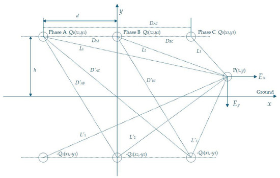
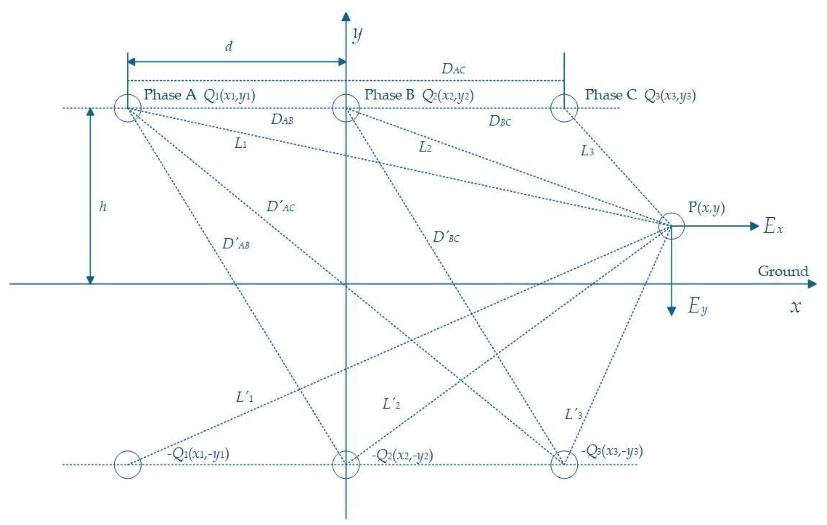
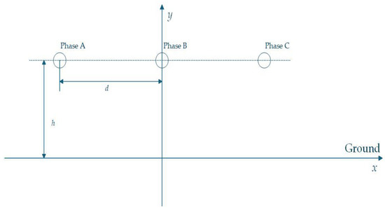
For two-dimensional transmission line models, simulated charges are typically set as infinite-length straight wire charges, with the number of charges generally exceeding one. The model employed in this paper is a two-dimensional three-phase horizontal transmission line. The schematic diagram of the spatial electric field calculated using the simulated charge method for this model is shown in Figure 1. d is the conductor distance. h is the height of the conductor. Q₁, Q₂, Q₃ are simulated charges. −Q₁, −Q₂, −Q₃ are their mirror charges.

$$P_{11}=P_{22}=P_{33}={\displaystyle \frac{1}{2\pi {\epsilon }_0}}ln\left({\displaystyle \frac{2h}{r_{eq}}}\right)$$

(1)

$$P_{12}={\displaystyle \frac{1}{2\pi {\epsilon }_0}}ln\left({\displaystyle \frac{D_{AB}^{\prime }}{D_{AB}}}\right)$$

(2)

$$P_{13}={\displaystyle \frac{1}{2\pi {\epsilon }_0}}ln\left({\displaystyle \frac{D_{AC}^{\prime }}{D_{AC}}}\right)$$

(3)

$$P_{23}={\displaystyle \frac{1}{2\pi {\epsilon }_0}}ln\left({\displaystyle \frac{D_{BC}^{\prime }}{D_{BC}}}\right)$$

(4)

Figure 1. Schematic diagram for solving spatial electric field strength.

[P] is a 3 × 3 potential coefficient matrix, where each element P_ij denotes the potential generated at the i-th (i = 1, 2, 3) boundary matching point by the j-th (j = 1, 2, 3) unit simulated charge. It is a known coefficient matrix completely determined by the geometric configuration of the system, and satisfies P_ij = P_ji. P_ii denotes the self-potential coefficient, and P_ij denotes the mutual-potential coefficient [13]. h is the height of the conductor above the ground. D_AB is the distance between the A-phase conductor and the B-phase conductor. D_AC is the spacing between Phase A conductor and Phase C conductor. D_BC is the distance between Phase B conductor and Phase C conductor. D′_AB is the distance between the mirror image of the A-phase conductor and the B-phase conductor. D′_AC is the distance between the mirror image of the A-phase conductor and the C-phase conductor. D′_BC is the distance between the mirror image of the phase B conductor and the phase C conductor. r_eq is the equivalent radius of conductors.

The horizontal component E_x, vertical component E_y, and spatial electric field strength E generated by each charge at point P are as follows:

$$E_x={\displaystyle \frac{1}{2\pi {\epsilon }_0}}{\displaystyle \sum _{k=1}^3{Q}_k}\left({\displaystyle \frac{x-x_k}{L_k^2}}-{\displaystyle \frac{x+x_k}{L_k^{\prime 2}}}\right)$$

(5)

$$E_y={\displaystyle \frac{1}{2\pi {\epsilon }_0}}{\displaystyle \sum _{k=1}^3{Q}_k}\left({\displaystyle \frac{y-y_k}{L_k^2}}-{\displaystyle \frac{y+y_k}{L_k^{\prime 2}}}\right)$$

(6)

$$E=\sqrt{E_x^2+E_y^2}$$

(7)

In the equation, Q_k denotes the simulated charge on conductor k. x_k is the horizontal coordinate of conductor k. y_k is the vertical coordinate of conductor k. L_k is the distance from conductor k to point P. L′_k is the distance from the mirror image of conductor k to point P.

2.2. Solution Process of the Simulated Charge Method

The main steps for solving the spatial electric field using the simulated charge method are:

(1)

Analyze the characteristics of the research subject, define the computational domain, and place n discrete simulated charges outside the computational domain to equivalently replace the original continuous charge distribution.

(2)

On a conductor with specified boundary conditions, establish matching points equivalent to the simulated charge quantity, where the potential at these matching points is known.

(3)

Based on the principle of electric field superposition, the potential at each matching point equals the sum of the potentials generated by all virtual charges acting upon it, forming a matrix-form system of potential equations:

$$\left[P\right]\left[Q\right]=\left[\phi \right]$$

(8)

(4)

[P] is the potential coefficient matrix and [φ] is the line voltage matrix. Solve the system of equations using mathematical methods to obtain the virtual charge matrices [Q].

(5)

Verify boundary conditions: Select additional monitoring points on the conductor surface to verify calculation accuracy. If precision requirements are not met, adjust the position, number, and configuration of simulated charges. Repeat steps until compliance is achieved.

(6)

Based on the validated simulated charge matrix [Q], determine the potential and electric field strength at any point in space.

3. Solving the Electric Field Inverse Problem with an Improved Genetic Algorithm

The forward problem model constructed using the simulated charge method reveals that the spatial electric field strength beneath a transmission line is determined by the amplitude and phase of its conductor voltage. The objective of the electric field inverse problem is to infer the voltage parameters of the conductors based on measured electric field strength values at several known locations. In practical applications, to better capture the spatial electric field distribution around transmission lines, the number of measurement points is typically greater than the number of simulated charges deployed. According to Equation (8), this is an overdetermined system. Directly solving this problem faces severe instability, manifested as non-uniqueness of solutions and extreme sensitivity to measurement noise [14]. Therefore, this problem can be reformulated as solving the following nonlinear optimization problem:

$$\underset{V}{min}\phi \left(V\right)={\displaystyle \sum _{m=1}^M‖E_m^{meas}-E_m^{cal}}{\left(V\right)‖}^2$$

(9)

In the equation, V = [V₁, θ₁, V₂, θ₂, ..., V_N, θ_N]^T denotes the voltage magnitude and phase vector of the N conductors to be inverted. $E_m^{meas}$ and $E_m^{cal}$ denote the measured electric field strength at the m-th (m = 1, 2, …, M) measurement point and the calculated value based on the simulated charge method, respectively. M is the total number of measurement points. For the least-squares problem in Equation (9), traditional gradient-based optimization algorithms are prone to getting stuck in local optima, making it difficult to obtain globally reliable solutions.

Genetic algorithms are meta-heuristic optimization algorithms that simulate the evolutionary processes found in nature, with their core principle rooted in “survival of the fittest”. Based on the principles of chromosome inheritance and natural selection, they mimic biological genetic evolution. Each numbered individual represents a solution, evaluated for quality by a fitness function. Through iterative rounds involving crossover and mutation operations, the algorithm converges toward an optimal solution [15,16,17]. Despite the advantages of genetic algorithms, such as their strong global search capability and independence from gradient information, they suffer from limitations including low computational efficiency, susceptibility to local optima, and sensitivity to model errors. Therefore, this paper adopts a genetic algorithm with global search capability as the solution framework and implements key improvements to address its shortcomings.

3.1. Constructing a Multi-Physics Constrained Tikhonov Regularization Objective Function

Constructing a priori knowledge of the power system as a regularization term and embedding it into the objective function transforms a purely data-driven problem into a constraint optimization problem guided by physical knowledge. The improved overall objective function is:

$$\underset{V}{min}\Psi \left(V\right)=\varphi \left(V\right)+\lambda R\left(V\right)$$

(10)

$$R\left(V\right)={\alpha }_1{R}_1\left(V\right)+{\alpha }_2{R}_2\left(V\right)+{\alpha }_3{R}_3\left(V\right)$$

(11)

In the equation, λ is the regularization parameter, which balances the weights of the data fitting term ϕ(V) and the regularization term R(V). The regularization term R(V) combines the voltage balance constraint term R₁(V), the phase symmetry constraint term R₂(V), and the magnitude prior constraint term R₃(V). α₁, α₂, and α₃ represent the respective weights of each constraint term.

The voltage balance constraint term R₁(V) is as follows:

$$\overline{U}={\displaystyle \frac{U_A+U_B+U_C}{3}}$$

(12)

$$R_1\left(V\right)={\displaystyle \frac{{\left(U_A-\overline{U}\right)}^2+{\left(U_B-\overline{U}\right)}^2+{\left(U_C-\overline{U}\right)}^2}{{\overline{U}}^2+\epsilon }}$$

(13)

In the formula, $\stackrel{-}{U}$ denotes the arithmetic mean of the three-phase voltage amplitudes. ε is a very small positive number used to prevent numerical instability in the formula when $\stackrel{-}{U}$ approaches zero. The denominator ${\overline{U}}^2$ is normalized to render this term a dimensionless relative error metric, preventing excessively large absolute voltage values from dominating the entire regularization term. For a normally operating three-phase AC system, the voltage amplitudes of each phase should be essentially equal. This constraint penalizes any deviation from the average value, compelling the optimization process to seek a voltage-balanced solution.

The phase symmetry constraint term R₂(V) is defined as follows:

$$\Delta {\phi }_{AB}=mod\left(\left({\phi }_A-{\phi }_B\right)+180,360\right)-180$$

(14)

$$\Delta {\phi }_{BC}=mod\left(\left({\phi }_B-{\phi }_C\right)+180,360\right)-180$$

(15)

$$\Delta {\phi }_{CA}=mod\left(\left({\phi }_C-{\phi }_A\right)+180,360\right)-180$$

(16)

$$R_2\left(V\right)={\displaystyle \frac{{(\Delta {\varphi }_{AB}-120)}^2+{(\Delta {\varphi }_{BC}-120)}^2+{(\Delta {\varphi }_{CA}+240)}^2}{K}}$$

(17)

In the formula, mod(x, y) denotes the modulo operation. The constant K serves as a normalization factor, scaling the phase error—measured in degrees squared—to a magnitude comparable to the dimensionless voltage balance constraint term. This ensures equal weighting of all terms during regularization. The constraint enforces a 120° symmetrical relationship among the three-phase voltages during inversion.

The amplitude prior constraint term R₃(V) is defined as follows:

$$R_3\left(V\right)={\displaystyle \frac{{\left(U_A-U_{rated}\right)}^2+{\left(U_B-U_{rated}\right)}^2+{\left(U_C-U_{rated}\right)}^2}{U_{rated}^2}}$$

(18)

In the formula, U_rated denotes the rated phase voltage of the system. Similar to the voltage balance constraint term, the denominator is normalized with ${\mathrm{U}}_{\mathrm{rated}}^2$ to make it a relative error metric. This constraint utilizes known line rated voltage information to guide the inversion results toward a reasonable engineering range.

λ is determined using trial-and-error combined with the L-curve criterion, aiming to balance the weights between the data fitting term and the physical constraint terms. The weights α₁, α₂, and α₃ are set based on the prior strength of each physical constraint: voltage balance and phase symmetry are strong priors under nominal operation, thus assigned higher weights (0.4). The magnitude prior is a weak prior, permitting actual voltages to deviate from rated values, hence receiving a lower weight (0.2). Specific values are determined through empirical tuning to ensure the objective function remains balanced and is not skewed by any single term’s excessive weight.

3.2. Multi-Start Optimization Strategy

To reduce reliance on a single initial population and avoid premature convergence, this improved algorithm independently executes multiple complete genetic optimization processes. Each iteration generates an initial population using a different random seed, from which the individual with the highest fitness is selected as the output for the global optimal solution.

In multi-start optimization strategies, determining the number of iterations requires striking an optimal balance between computational efficiency and inversion accuracy. Although experiments involve multiple changes in the number of iterations, it was found that when the number of iterations increased from 1 to 3, the runtime increased from 7.34 s to 12.29 s, with an error margin of less than 5%. However, when the number of iterations increased from 3 to 5, the runtime increased from 12.29 s to 17.26 s, with no significant change in inversion accuracy. Moreover, the inverse problem addressed in this paper involves a six-dimensional parameter space, namely the magnitude and phase of the three-phase voltages. Each of these parameters has well-defined physical constraints. The phase constraints satisfy the three-phase symmetry relationship. By designing a differentiated initial population strategy, three independent runs can systematically cover the primary feature regions of the solution space: the first run focuses its search around the rated values, the second run emphasizes exploration of boundary regions, and the third run performs fine-tuning based on the results from the previous searches. Therefore, the number of runs is designed as three.

3.3. Initial Population Generation for Diversity

Abandoning fully random initialization, the initial population is generated within feasible upper and lower bounds of the set voltage amplitude and phase, thereby providing directional guidance for inversion results. For instance, when Phase A of a three-phase transmission line operates normally at 0° phase angle, the initial population is randomly generated within a certain range around this phase angle. This initialization based on prior knowledge enables the algorithm to commence its search from positions closer to real-world physical conditions, enhancing initial search efficiency and convergence speed.

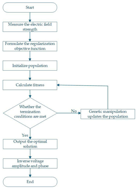
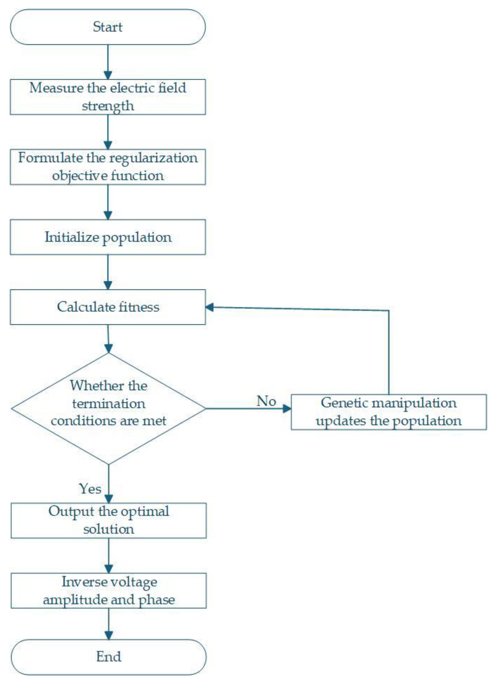
Figure 2 shows the main flowchart of the inversion process.

Figure 2. Main flowchart of inversion.

4. Single-Circuit Three-Phase Horizontal Transmission Line Example

4.1. Nominal Balanced Operation

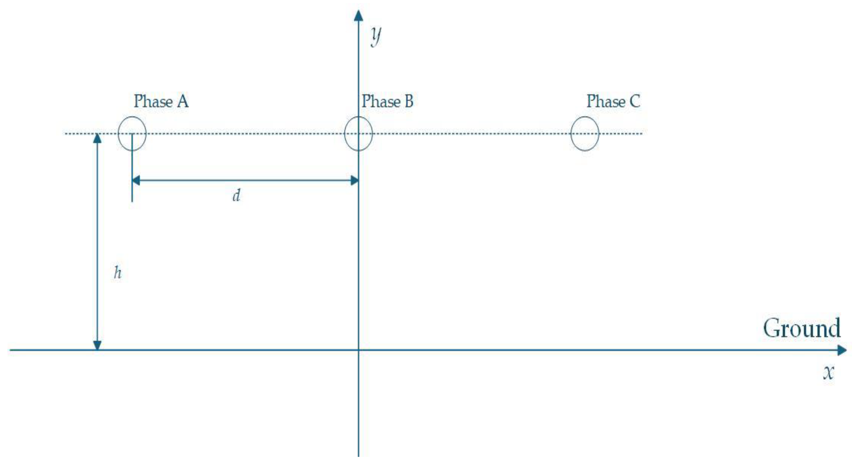
Taking a single-circuit three-phase horizontal transmission line with a two-dimensional line voltage of 500 kV as an example for calculation, the schematic diagram of the model is shown in Figure 3.

Figure 3. Single-circuit three-phase horizontal transmission line model.

The conductor height h and conductor spacing d in Figure 3 are taken as 12.19 m and 13.72 m, respectively. The geometric radius R of the quadruple conductor is 0.323 m, and the secondary conductor radius r is 0.0148 m. With the x-axis representing the ground, calculations neglect the effects of conductor sag and lightning arresters, idealizing the transmission line as an infinitely long straight conductor.

Based on the aforementioned model parameters and Equations (1)–(4), the equivalent radius r_eq and the potential coefficient matrix [P] can be calculated:

$$r_{eq}=R\sqrt[n]{{\displaystyle \frac{nr}{R}}}=0.323\times \sqrt[4]{{\displaystyle \frac{4\times 0.0148}{0.323}}}=0.2113\mathrm{m}$$

(19)

$$\left[P\right]=\left[\begin{array}{ccc}8.5312& 1.2704& 0.5168\\ 1.2704& 8.5312& 1.2704\\ 0.5168& 1.2704& 8.5312\end{array}\right]\times {10}^{10}$$

(20)

The three-phase line voltage is 500 kV. Considering voltage fluctuations in actual scenarios, a certain overvoltage margin must be maintained. Therefore, the three-phase voltages are as follows:

$$U_{\varphi }={\displaystyle \frac{U_L}{\sqrt{3}}}\times 1.05$$

(21)

$$\left[\begin{array}{c}{\dot{U}}_A\\ {\dot{U}}_B\\ {\dot{U}}_C\end{array}\right]=\left[\begin{array}{c}303\angle 0°\\ 303\angle 120°\\ 303\angle -120°\end{array}\right]\mathrm{kV}$$

(22)

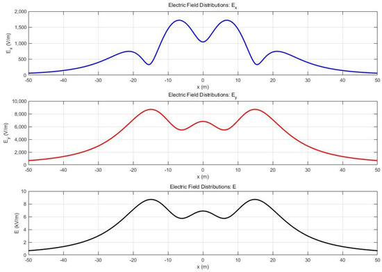
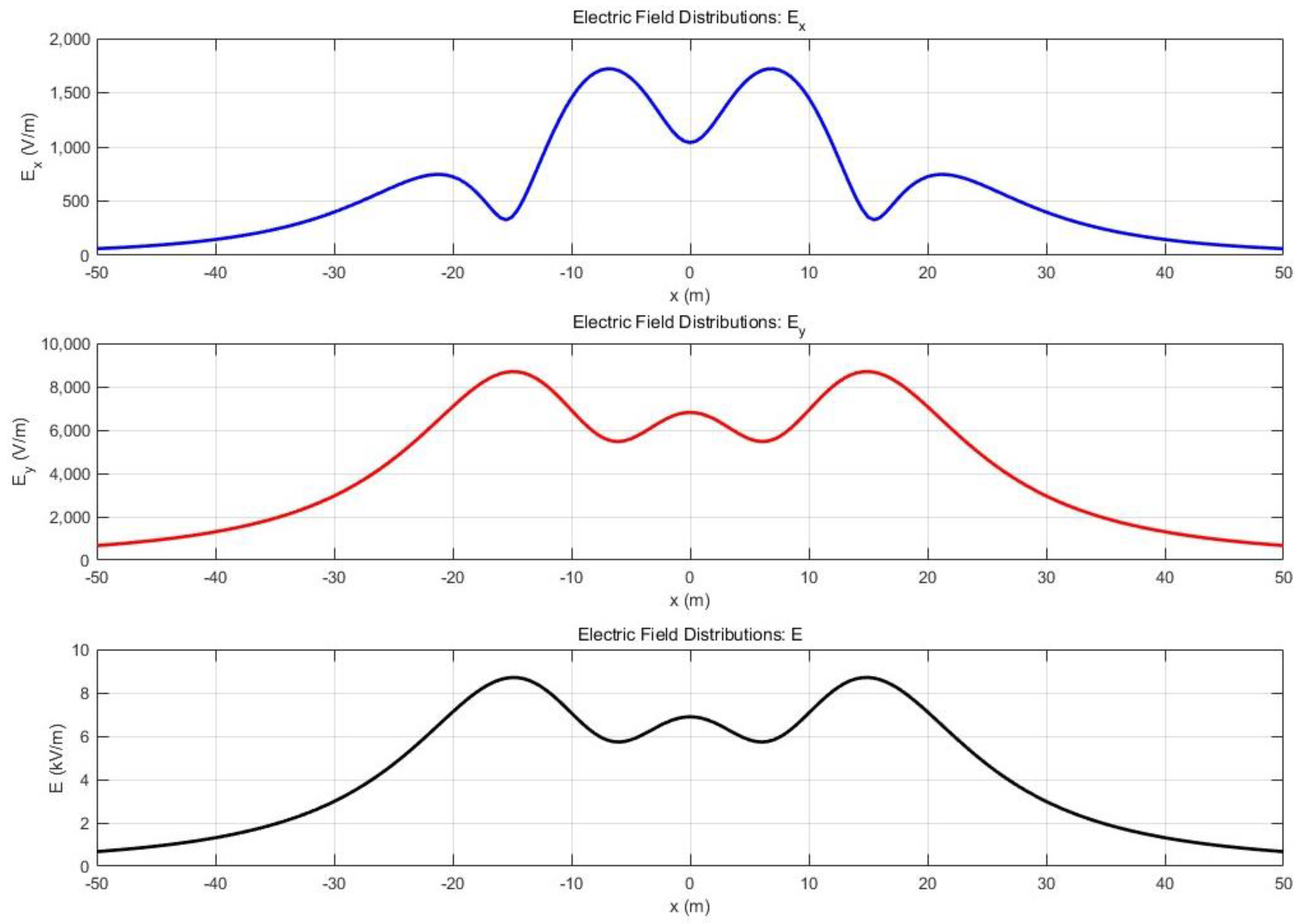
As documented in references [18,19,20], electric fields can impact human health, necessitating attention to the electric field strength near ground level beneath transmission lines. Portable electric field measurement devices can be used during worker operations. Wristband-style devices minimally disrupt work activities. Considering adult height, a height of 1.5 m is deemed appropriate for calculation purposes. Therefore, the spatial electric field strength distribution at this height is computed. Based on Equations (5)–(7), the horizontal coordinate range is set from −50 m to 50 m with a step size of 0.5 m. Figure 4 is the spatial electric field intensity distribution at a height of 1.5 m above ground level that is calculated and plotted by using MATLAB r2024a.

Figure 4. Calculated values of spatial electric field strength distribution.

Using Maxwell 2024r2 software, a two-dimensional model was established as shown in Figure 3. Observation points were set at 5 m intervals from −20 m to 20 m. The simulated electric field strength values measured at these observation points were compared with the calculated values. Table 1 shows the results.

Table 1. Comparison of simulated and calculated electric field strength values at each observation point.

Position	Simulation Value	Calculated Value	Difference
−20 m	7.22 kV/m	7.12 kV/m	1.40%
−15 m	8.79 kV/m	8.71 kV/m	0.92%
−10 m	7.15 kV/m	7.23 kV/m	1.11%
−5 m	5.86 kV/m	5.96 kV/m	1.34%
0 m	7.09 kV/m	7.12 kV/m	0.42%
5 m	5.83 kV/m	5.96 kV/m	2.18%
10 m	7.13 kV/m	7.23 kV/m	1.38%
15 m	8.75 kV/m	8.71 kV/m	0.46%
20 m	7.23 kV/m	7.12 kV/m	1.54%

By comparing the simulated values and calculated values at each observation point, the error is found to be within 5%. Therefore, in the numerical inversion experiments, a 5% random noise is added to the theoretically calculated values to simulate the measurement errors that inevitably exist in actual measurements. This approach tests the stability and engineering applicability of the inversion algorithm.

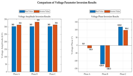
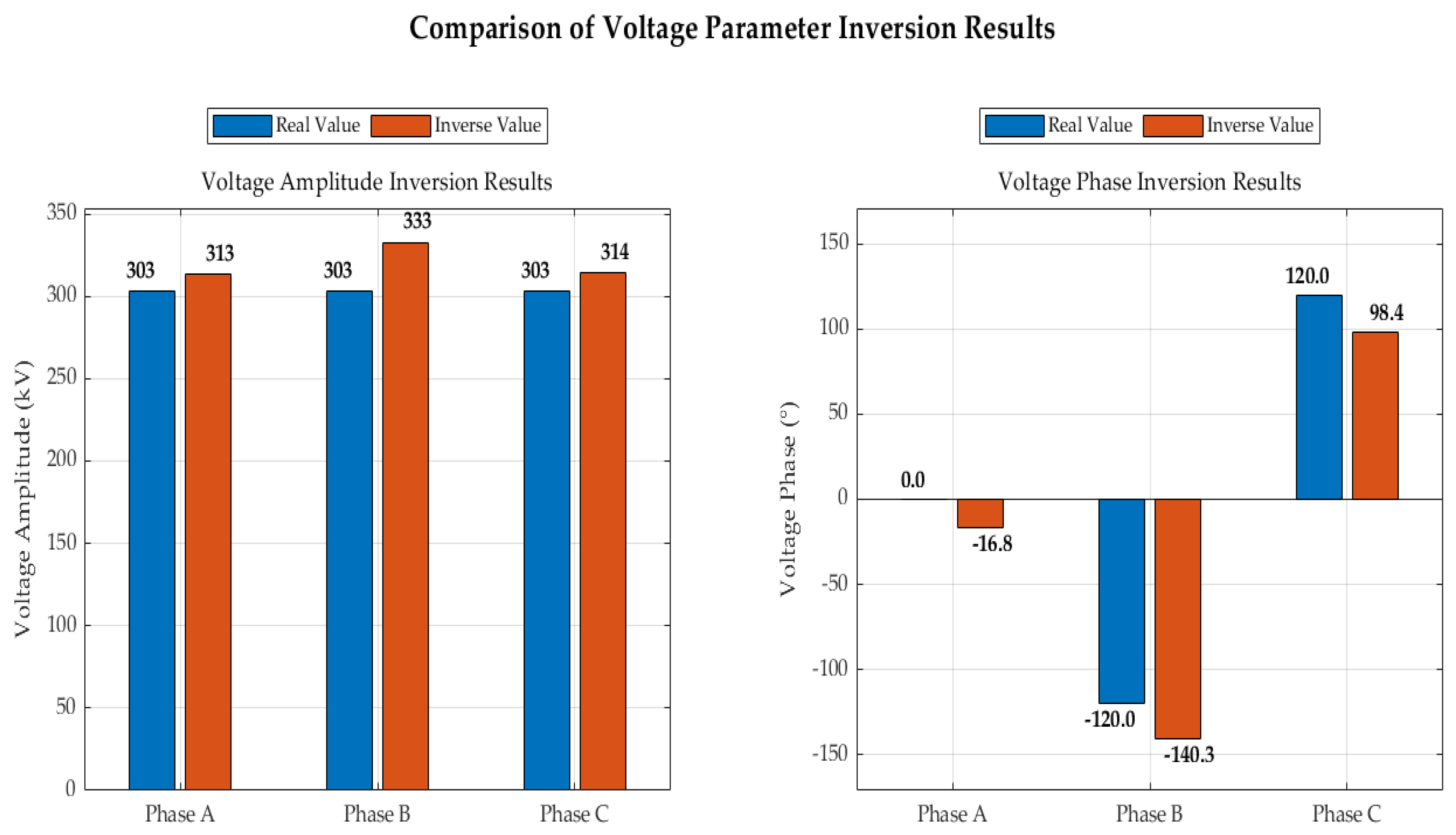
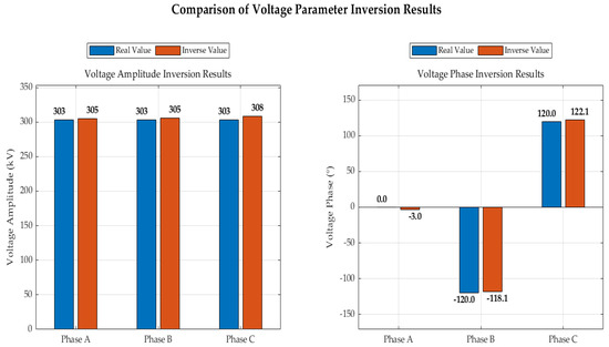
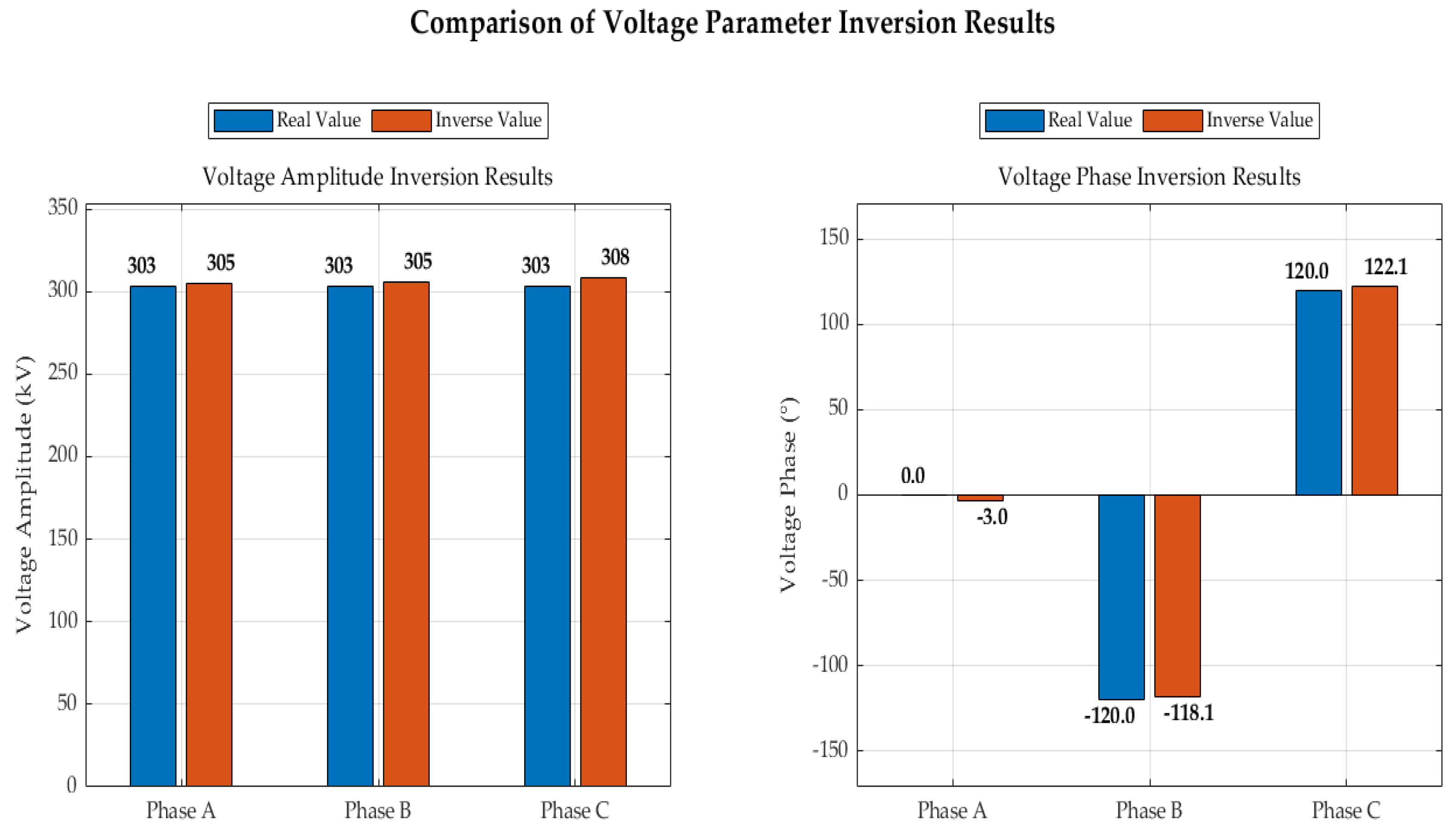
Figure 5 is the traditional genetic algorithm inversion results. Figure 6 is the improved genetic algorithm inversion results. When using traditional genetic algorithms for inversion, voltage amplitude is reliable but phase deviates significantly. In contrast, the improved genetic algorithm delivers reliable voltage amplitude and phase with better stability. The traditional genetic algorithm took 7.34 s, while the improved genetic algorithm took 12.29 s. The improved genetic algorithm significantly increases the probability of finding the global optimum solution at the cost of relatively manageable computational overhead.

Figure 5. Traditional genetic algorithm inversion results.

Figure 6. Improved genetic algorithm inversion results.

Under identical conditions, running the improved genetic algorithm inversion ten times yielded identical amplitude and phase inversion results each time, consistent with those shown in Figure 6.

4.2. Sensitivity Analysis of Regularization Parameters

To evaluate the impact of the regularization parameter λ and constraint weights α₁, α₂, and α₃ on inversion results, a sensitivity analysis was conducted. While keeping other parameters constant, λ was varied within the range of 0.008 to 0.012, and each weight was adjusted within ±50%. Changes in voltage amplitude error and phase error were observed. The results are shown in Table 2. As shown in Table 2, when λ = 0.01, α₁ = 0.4, and α₂ = 0.4, both amplitude and phase errors are relatively small. When only λ or α₁ or α₂ is altered, both amplitude and phase errors increase.

Table 2. Regularization Parameter Sensitivity Analysis Results.

λ	α1	α2	α3	Amplitude Error	Phase Error
0.008	0.4	0.4	0.2	2.31%	4.5°
0.009	0.4	0.4	0.2	1.65%	2.6°
0.01	0.4	0.4	0.2	1.65%	2.1°
0.0011	0.4	0.4	0.2	2.97%	4.1°
0.0012	0.4	0.4	0.2	2.97%	6.8°
0.01	0.2	0.4	0.2	2.97%	6.4°
0.01	0.6	0.4	0.2	1.65%	3.0°
0.01	0.4	0.2	0.2	2.31%	15.2°
0.01	0.4	0.6	0.2	4.95%	2.3°

4.3. Analysis of the Impact of Different Noise Levels

To systematically evaluate the algorithm’s performance under varying noise levels, inversion experiments were conducted under additional Gaussian noise conditions of 1%, 3%, and 10%, supplementing the original 5% noise level. Amplitude errors and phase errors were compared across different noise levels, with results presented in Table 3.

Table 3. Inversion Error at Different Noise Levels.

Noise Level	Amplitude Error	Phase Error
1%	0.33%	3.7°
3%	1.32%	0.8°
5%	1.65%	2.1°
10%	4.95%	8.1°

The results indicate that as the noise level increases from 1% to 10%, the amplitude error rises to 4.95% and the phase error increases to 8.1°. However, even at 10% noise, the errors remained within acceptable limits, demonstrating the method’s robust noise resistance. Notably, the amplitude and phase errors did not strictly increase proportionally with noise level. At just 1% noise, the phase error exceeded the noise level, indicating a need for further optimization in future work.

4.4. Analysis of the Impact of Different Numbers of Observation Points

To systematically evaluate the algorithm’s performance under varying numbers of observation points, inversion results were tested using 5, 7, 9, 11, and 13 observation points, as shown in Table 4.

Table 4. Inversion Error at Different Numbers of Measurement Points.

Number of Observation Points	Amplitude Error	Phase Error
5	1.65%	4.3°
7	1.65%	2.9°
9	1.65%	2.1°
11	1.36%	1.6°
13	0.66%	1.6°

Results indicate that as the number of observation points increases from 5 to 13, both amplitude and phase errors gradually decrease. Beyond a certain threshold, no significant improvement is observed, necessitating practical considerations when determining the optimal sensor configuration.

5. Conclusions

This paper proposes an improved genetic algorithm incorporating multi-physical constraint regularization, effectively addressing the instability and noise sensitivity issues in non-contact voltage inversion for transmission lines under nominal balanced operating conditions. By structuring physical knowledge, such as voltage balance, phase symmetry, and amplitude priors, into regularization terms and integrating a multi-start optimization strategy, the stability and reliability of the inversion algorithm are significantly enhanced. Numerical simulations demonstrate that under 5% measurement noise conditions, this method achieves voltage magnitude inversion errors below 5% and phase errors less than 5°, exhibiting significantly enhanced interference resistance compared to conventional approaches. The current work is specifically validated for balanced three-phase systems. Its applicability to unbalanced or asymmetric scenarios requires further investigation. This technique provides an effective non-contact measurement solution for achieving high-precision, high-reliability transmission line condition monitoring, offering a novel technological pathway for digital operation and maintenance in smart grids. Future research will extend the method to unbalanced conditions, incorporate 3D line geometry effects, and explore adaptive regularization parameter selection.

In subsequent studies, we plan to employ Monte Carlo simulations to conduct a comprehensive uncertainty analysis. This analysis will encompass random variations in sensor locations, conductor sag (modeled using three-dimensional catenary curves), geometric tolerances, and variable geological conditions such as soil electrical conductivity and dielectric constant. We believe these efforts will further enhance the engineering application maturity of the proposed inversion technique.

References

- Zhang, Y.; Li, T.; Liu, X.; Huang, Z.; Li, Q. Multi-Port Collaborative Control Strategy with Smooth Operational Transitions for Photovoltaics, Energy Storage, Direct Current, and Flexibility System. IEEE Trans. Power Electron. 2025, 40, 11715–11724. [Google Scholar] [CrossRef] [Scilit]
- Dong, C.; Wang, J.; Li, X.; Jin, C.; Jiang, W.; Zhang, Z.; Jia, H. Synthetic Resilience Exploration and Economic Defense Strategy for Microgrid-Level AC/DC Hybrid Energy System. IEEE Trans. Power Electron. 2023, 38, 2565–2576. [Google Scholar] [CrossRef] [Scilit]
- Nigam, A.; Lee, D.-C. Enhanced Seamless Transition Control of Grid-Tied Converters Using Dual-eSOGI Vector-Based Synchronization Under Grid Faults. IEEE Trans. Power Electron. 2025, 40, 13952–13964. [Google Scholar] [CrossRef] [Scilit]
- Li, Y.; Chen, W.; Li, K.; Qi, B.; Huang, S.; Xiang, N. A Non-Contact Transient Voltage Inference Method Based on Multi-Fidelity Data Fusion. IEEE Trans. Instrum. Meas. 2025, 74, 9007911. [Google Scholar] [CrossRef] [Scilit]
- Xing, Y.; Liu, J.; Li, F.; Zhang, G.; Li, J. Non-Contact Voltage Reconstruction Method Based on Dual-Pin Type Probes Structure and Measuring Point Optimization for AC Overhead Transmission Lines. IEEE Trans. Instrum. Meas. 2024, 73, 1501312. [Google Scholar] [CrossRef] [Scilit]
- Gao, J.; Wu, S.; Liu, X.; Xu, C.; Ma, H.; Xin, M.; Zhang, H.; Feng, C.; Bi, R.; Hu, J. Research on Non-Contact Voltage Measurement for Insulated Transmission Line. In Proceedings of the 2023 3rd International Conference on Energy Engineering and Power Systems (EEPS), Dali, China, 28–30 July 2023; pp. 624–627. [Google Scholar] [CrossRef] [Scilit]
- Wang, J.; Yan, X.; Zhong, L.; Zhu, X. Simulation and Test of a Contactless Voltage Measurement Method for Overhead Lines Based on Reconstruction of Integral Node Parameters. Sensors 2020, 20, 246. [Google Scholar] [CrossRef] [Scilit] [PubMed]
- Zhang, J.; Tan, Z.; Xu, Z.; Liu, Z.; Tian, B.; Wang, Z.; Lv, Q.; Luo, B.; Liu, X.; Hu, J. A Novel Optimized Gauss Integral for Transmission Line Voltage Measurement. In Proceedings of the 2022 IEEE 6th Conference on Energy Internet and Energy System Integration (EI2), Chengdu, China, 11–13 November 2022; pp. 1638–1643. [Google Scholar] [CrossRef] [Scilit]
- Zhang, Z.; Liu, Z.; Geng, P.; Ma, Y. Research on the Three-Phase Voltage Inversion Algorithm of Transmission Lines Based on Electric Field Coupling. In Proceedings of the 2024 6th Asia Energy and Electrical Engineering Symposium (AEEES), Chengdu, China, 28–31 March 2024; pp. 42–47. [Google Scholar] [CrossRef] [Scilit]
- Xiao, D.; He, T.; Zhao, W.; Du, X.; Xie, Y. Improved Three-Dimension Mathematical Model for Voltage Inversion of AC Overhead Transmission Lines. IEEE Access 2019, 7, 166740–166748. [Google Scholar] [CrossRef] [Scilit]
- Jiao, X.; Huang, M.; Cheng, G.; Liu, Z. An Improved Niche Genetic Algorithm for Solving Job Shop Scheduling Problem. In Proceedings of the 2025 IEEE 13th International Conference on Computer Science and Network Technology (ICCSNT), Harbin, China, 18–19 October 2025; pp. 1–3. [Google Scholar] [CrossRef] [Scilit]
- Xia, Z. Application of Improved Genetic Algorithm in Intelligent Network Technology for Enterprise Financial Security. In Proceedings of the 2024 International Conference on Intelligent Algorithms for Computational Intelligence Systems (IACIS), Hassan, India, 23–24 August 2024; pp. 1–6. [Google Scholar] [CrossRef] [Scilit]
- Chen, W.; Chang, J.; Lin, F.; Song, H.; Wu, X. Improved Charge Simulation Method for Overhaul Robot Energized Maintenance of Disconnect Switches. In Proceedings of the 2023 6th International Conference on Energy, Electrical and Power Engineering (CEEPE), Guangzhou, China, 12–14 May 2023; pp. 196–200. [Google Scholar] [CrossRef] [Scilit]
- Widdershoven, R.; Vervliet, N.; De Lathauwer, L. A Bézoutian-Based Method for Solving Overdetermined Systems of Polynomial Equations. In Proceedings of the 2024 32nd European Signal Processing Conference (EUSIPCO), Lyon, France, 26–30 August 2024; pp. 1352–1356. [Google Scholar] [CrossRef] [Scilit]
- Feng, J.; He, Y.; Pan, Y.; Zhou, Z.; Chen, S.; Gong, W. Enhancing Fitness Evaluation in Genetic Algorithm-Based Architecture Search for AI-Aided Financial Regulation. IEEE Trans. Evol. Comput. 2024, 28, 623–637. [Google Scholar] [CrossRef] [Scilit]
- Yao, Y.; Yang, Y.; Tian, Y.; Song, X.; Yang, M.; Sun, J.; Dai, J. Improved Genetic Algorithm-Based MEP Search Strategy for DSNs Intrusion Detection. IEEE Sens. J. 2024, 24, 33544–33559. [Google Scholar] [CrossRef] [Scilit]
- Souza, M.G.; Vallejo, E.E.; Estrada, K. Detecting Clustered Independent Rare Variant Associations Using Genetic Algorithms. IEEE/ACM Trans. Comput. Biol. Bioinform. 2021, 18, 932–939. [Google Scholar] [CrossRef] [Scilit] [PubMed]
- Chen, K.-L.; Chen, H.-S. Implementation and Feasibility of Environmental Electric Field Measurement Based on Unmanned Aerial Vehicle. IEEE Trans. Power Deliv. 2024, 39, 1877–1888. [Google Scholar] [CrossRef] [Scilit]
- Yang, Z.; He, D.; Ding, L. The Optimization Study for Electromagnetic Radiation with Ultrahigh Voltage Transmission Lines. IEEE Trans. Electromagn. Compat. 2022, 64, 1480–1492. [Google Scholar] [CrossRef] [Scilit]
- Li, X.; He, W.; Tang, Y.; Gao, S.; Xie, Y.; Liu, Y.; Li, Y.; Zhao, H. Research on the Induced Electric Field of Human under EHV AC Transmission Lines Based on BAS-CSM Algorithm. In Proceedings of the 2023 IEEE International Conference on Power Science and Technology (ICPST), Kunming, China, 5–7 May 2023; pp. 1009–1014. [Google Scholar] [CrossRef] [Scilit]
Disclaimer/Publisher’s Note: The statements, opinions and data contained in all publications are solely those of the individual author(s) and contributor(s) and not of MDPI and/or the editor(s). MDPI and/or the editor(s) disclaim responsibility for any injury to people or property resulting from any ideas, methods, instructions or products referred to in the content. |
© 2026 by the authors. Licensee MDPI, Basel, Switzerland. This article is an open access article distributed under the terms and conditions of the Creative Commons Attribution (CC BY) license.