Design and Validation of a Multimodal Environmental Monitoring System Based on Sensors and Artificial Intelligence

Abstract

Reliable and real-time environmental monitoring is essential for controlling pollution and protecting public health. However, conventional station-based measurements are expensive and often lack spatial and temporal resolution. This paper proposes a low-cost multimodal environmental monitoring system. Experiments verified that thin-film thermocouples exhibit near-linear voltage–temperature characteristics ($R^2>0.99$). Integration of the AI data pipeline substantially enhances monitoring accuracy: the proposed fusion strategy reduces relative error to approximately 2.3% under typical noise conditions, with a correlation coefficient of 0.79 between predicted and observed PM2.5 values. This research provides a scalable blueprint for edge-deployable environmental monitoring. A thin-film thermocouple with a fast response time is used as a temperature sensor and is statically calibrated against a K-type reference. To improve dynamic tracking and reduce measurement noise, a Kalman filter-based fusion strategy is employed, which is then compared with weighted averaging and Bayesian fusion. Simulation-driven validation is performed for thermocouple linearity, PID-based temperature control, micro-signal filtering and system-level latency and robustness. The results demonstrate that thin-film thermocouples exhibit near-linear voltage–temperature characteristics (R² > 0.99) with Seebeck coefficients ranging from 40.92 to 42.08 μV/°C, close to the theoretical K-type value of 42.87 μV/°C. The proposed fusion strategy reduces relative error to ~2.3% under typical noise conditions, enabling stable, real-time processing with near-second latency for 10,000-point batches. This study summarizes the design considerations for selecting and calibrating sensors and for achieving AI robustness in the presence of drift and faults. It provides a scalable blueprint for edge-deployable environmental monitoring.

1. Introduction

Environmental pollution and climate change have intensified the demand for real-time, accurate, and cost-effective monitoring of air and water quality. While high-grade monitoring stations provide reliable measurements, their installation and maintenance costs limit deployment density and lead to coarse spatial coverage. Low-cost sensors and embedded systems enable dense and mobile sensing, but their outputs are affected by cross-sensitivity, drift, and noise. These limitations motivate the integration of artificial intelligence (AI) for calibration, fusion, and prediction.

Related work indicates a clear evolution from basic data collection toward intelligent perception. For example, Alvear et al. [1] proposed a mobile pollution sensing architecture integrating low-end sensors, smartphones, and cloud services, emphasizing calibration and variability reduction. AI methods such as genetic algorithm (GA) [2,3,4,5] optimization and artificial neural networks (ANNs) [6,7,8,9] have been used to improve prediction and classification in embedded scenarios. Moreover, metaheuristic-assisted [10,11,12] feature selection and deep models have been deployed on edge platforms for real-time decision-making in complex sensing environments. Conventional sensors frequently encounter issues of non-linear drift and cross-interference in complex environments [13,14]. By contrast, AI-assisted systems can significantly enhance detection sensitivity and classification accuracy through multi-feature fusion and deep learning, enabling low-cost sensors to achieve the performance of professional-grade monitoring stations in specific applications [15,16,17,18,19]. We have clarified our “physics-data joint driven” architecture. The text now emphasizes how high-speed temperature sensing provides micro-level compensation to the MOS gas sensor array, effectively reducing dynamic errors induced by sensor inertia.

In China, sensor–AI environmental monitoring has expanded from air quality to multi-media monitoring (water, soil, and noise), and research increasingly targets urban-scale prediction, early-warning, and decision support. However, key challenges remain: (i) sensor heterogeneity and cross-response causing unreliable raw measurements; (ii) dynamic errors induced by sensor inertia and slow response; (iii) limited robustness under abnormal data and sensor failures; and (iv) insufficient generalization of AI models across regions and seasons.

The main contributions of this paper are:

• A modular environmental monitoring architecture supporting air-quality, water-quality, and temperature sensing with a unified AI data pipeline.
• A thin-film thermocouple calibration workflow including linearity, Seebeck coefficient consistency, and implications for temperature compensation.
• A comparative evaluation of fusion strategies (weighted averaging, Kalman filtering, Bayesian fusion) and their effects on error reduction.
• System-level simulation results on latency, robustness, and model generalization, providing guidance for real-time edge deployment.

2. Materials and Methods

2.1. System Architecture and Data Flow

The proposed system follows an edge-to-cloud workflow. At the edge, sensing nodes acquire air and water quality and temperature signals via analogue front-end circuits and/or digital interfaces. This is followed by analogue-to-digital converter (ADC) sampling and timestamping on a microcontroller unit (MCU). Following signal conditioning (gain and offset removal and low-pass filtering), the MCU carries out lightweight preprocessing and transmits features and/or raw samples to an upper-layer processor or cloud server. In the cloud (or on an edge gateway), AI modules then carry out data cleaning, normalization, multi-sensor fusion, anomaly detection and short-term forecasting. The pipeline supports real-time dashboards and offline analytics.

The system employs a phased fusion architecture: edge-side execution handles feature-level fusion, integrating resistance changes from multiple gas sensors into response vectors; cloud-side execution performs decision-level fusion, utilizing temperature-corrected water quality and air characteristics for joint environmental quality assessment.

2.2. Sensor Modules and Physical Principles

The selection of sensors aims to strike a balance between cost, deployability and data quality. Air-quality monitoring uses an array of MOS gas sensors to provide multidimensional response signatures for gases and VOCs. Water-quality monitoring uses dedicated probes to measure pH, dissolved oxygen (DO), turbidity and conductivity. Temperature monitoring relies on thin-film thermocouples for a fast response and to compensate for the temperature of other sensors. The sensing modes and typical specifications are summarized in Table 1.

Table 1. Summary of sensing modalities and typical specifications.

Modality	Target Parameter (s)	Principle/Sensor Type	Typical Range	Notes
Air	CO, NOx, SO2, VOCs, PM2.5 *	MOS sensor array (e.g., MQ-135, SGP30, BME680, CCS811)	1–1000 ppm (gas) **	Fast response (1–10 s); cross-sensitivity mitigated by AI
Water	pH	Glass electrode (Nernst equation)	0–14	Typical accuracy ±0.01 pH with calibration
Water	Dissolved oxygen (DO)	Clark polarographic electrode	0–20 mg/L	Requires temperature/pressure compensation
Water	Turbidity	90° nephelometry)	<0.05–400 NTU	Infrared light source recommended for reduced colour interference
Water	Conductivity	Four-electrode conductivity probe	0–2000 μS/cm (typ.)	Avoids polarization; temperature compensation needed
Temperature	Ambient/probe temperature	Thin-film thermocouple (Seebeck effect)	20–100 °C (tested)	Suitable for compensation and heater control

* PM2.5 is typically measured using optical scattering sensors; here it is also treated as an AI-predicted indicator when direct particulate sensing is unavailable. ** Exact ranges depend on sensor type and calibration.

2.2.1. Air-Quality Sensing Using MOS Sensor Arrays

To address cross-sensitivity issues in MOS arrays, supervised learning algorithms such as random forests are employed to map response features onto concentration metrics. MOS sensors exploit conductivity changes in gas-sensitive materials (e.g., SnO₂, ZnO, WO₃) at elevated temperatures. In clean air, oxygen adsorbs on the surface and captures conduction electrons, increasing resistance. Reducing gases (e.g., CO, VOCs) react with adsorbed oxygen species, releasing electrons and decreasing resistance; oxidizing gases (e.g., NO₂) further extract electrons and increase resistance. Specifically, we describe how temperature affects the resistance–concentration relationship in MOS sensors via the power law $R_s=R_0{\left(C/C_0\right)}^{-\alpha }$ and how it influences electrochemical potential in pH electrodes according to the Nernst equation:

$$E=E_0-{\displaystyle \frac{2.303RT}{F}}\cdot \mathrm{pH}$$

The thin-film thermocouple provides the temperature T required for these corrections.

In a voltage divider, the output voltage is

Vout = Vc · RL/(Rs + RL)

To mitigate cross-sensitivity, a response vector X = [R1/R01, R2/R02, …, Rn/R0n]^T is formed using an array of sensors. Dimensionality reduction techniques (e.g., principal component analysis (PCA)) and supervised learning techniques (e.g., support vector machines (SVM) and random forest) map response signatures to gas categories and/or concentrations. Temperature-dependent drift can be mitigated using compensation models and periodic calibration.

2.2.2. Water-Quality Sensing

Water-quality sensing involves compensating for non-linear drift in pH and dissolved oxygen (DO) sensors through AI algorithms. pH and DO were selected as core parameters due to their direct reflection of a water body’s biochemical state. This sensor module is designed to support real-time anomaly detection in surface water, freshwater resources, and wastewater treatment processes. A pH glass electrode follows the Nernst equation (25 °C):

E = E0 − (2.303 RT/F) · pH ≈ E0 − 59.16 mV · pH

A Clark-type dissolved oxygen (DO) sensor generates a diffusion current that is proportional to the oxygen concentration and is consistent with Faraday’s law. Turbidity is measured using nephelometry (90° scattered light), in accordance with, and the results are expressed in nephelometric turbidity units (NTU). Conductivity is measured using a four-electrode probe to minimize polarization, and is normalized to 25 °C with an associated temperature coefficient of approximately 0.02/°C.

2.2.3. Thin-Film Thermocouple Temperature Sensing

Thin-film thermocouples exploit the Seebeck effect: two dissimilar conductors produce a thermoelectric voltage proportional to the temperature difference between the hot and reference junctions. For moderate spans, a linear approximation is used:

EAB ≈ SAB · (Thot − Tcold)

In this study, thin-film thermocouples were calibrated within the range of 20–100 °C against a K-type reference, in order to obtain sample-specific SAB values and the quality of the linear fit (R²). The calibrated temperature signal is then used for compensation and PID temperature control experiments.

2.3. AI-Enabled Data Processing and Fusion

The AI pipeline comprises three layers: (1) Data cleansing layer: Outliers are removed using the 3σ criterion. (2) Feature extraction layer: PCA is employed to reduce the dimensionality of the N-dimensional response vectors from the MOS array, retaining over 95% of the variance information. (3) Decision layer: A random forest classifier is configured with 100 decision trees and a maximum depth of 15 to prevent overfitting on small sample datasets.

2.3.1. Preprocessing and Feature Extraction

The first layer focuses on signal conditioning at the edge. Raw data from heterogeneous sensors undergo outlier removal using the $3\sigma$ rule to eliminate impulsive noise. Following normalization (Min-Max or Z-score), the system performs feature extraction. For the MOS gas sensor array, principal component analysis (PCA) is employed to reduce the $N$-dimensional response vector into a lower-dimensional space while preserving over 95% of the variance information. This dimensionality reduction mitigates cross-sensitivity and reduces the computational load for subsequent stages.

2.3.2. Hybrid Fusion Strategy

The system employs a hybrid fusion strategy, distinguishing between feature-level and decision-level fusion to optimize data utility:

Feature-level Fusion (Edge): Carried out at the sensing node, this stage integrates multi-dimensional responses from sensor arrays (e.g., MOS gases) to form signature vectors.

Decision-level Fusion (Cloud): Conducted on the server or edge gateway, this stage aggregates processed data from air, water, and temperature modules to perform holistic environment assessment. A random forest classifier, configured with 100 decision trees and a maximum depth of 15 to prevent overfitting, maps these integrated features to specific pollutant concentrations.

2.3.3. Dynamic Optimal Estimation and Uncertainty Handling

To address sensor noise and environmental dynamics, two advanced fusion algorithms are implemented:

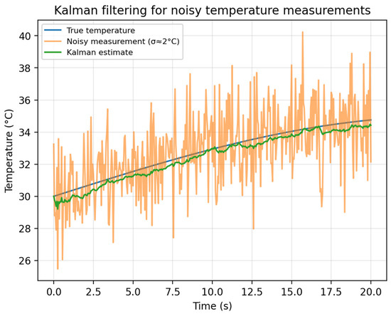
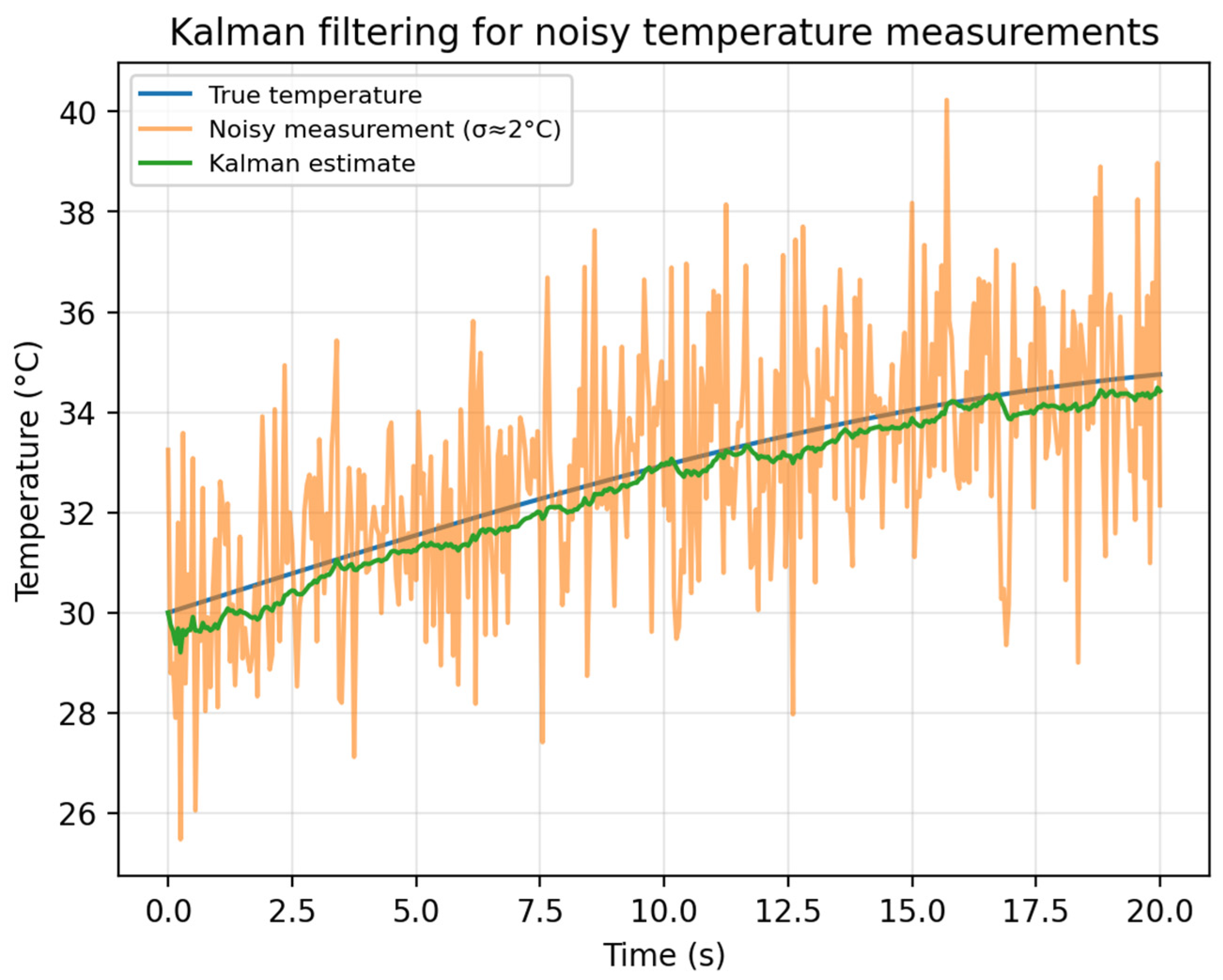
Kalman Filtering: For linear Gaussian dynamics, a recursive Kalman filter provides a minimum-variance estimator. In simulation settings, this approach suppresses high-frequency measurement noise while tracking slow environmental changes, achieving a relative error as low as ~2.3%.

Bayesian Fusion and Anomaly Detection: Bayesian fusion combines sensor likelihoods with prior information to produce a posterior estimate. Crucially, this method provides an explicit measure of uncertainty. By monitoring the posterior probability distribution, the system can identify sensor faults or drift; readings with a low probabilistic likelihood are flagged as anomalies, enabling robust aggregation even under partial sensor failure.

2.3.4. Temperature Compensation Mechanism

Leveraging the fast response of thin-film thermocouples, the pipeline applies microsecond-level temperature compensation. By incorporating real-time temperature T into the analytical models (e.g., the Nernst equation for pH or power-law models for MOS resistance), the system dynamically corrects for thermal drift, ensuring measurement stability across varying environmental conditions.

2.4. Simulation and Calibration Setup

Prior to full hardware integration, MATLAB-style simulations are employed to validate the core modules and analyse the controller response, filter behaviour, fusion comparison and robustness. Benchtop calibration experiments are performed on the thin-film thermocouple, for which an alcohol lamp serves as the heat source and a calibrated K-type thermocouple serves as the reference. The thermoelectric voltage is collected at temperatures between 20 and 100 °C in intervals of 10 °C. Linear regression is then applied to determine SAB and R². A comparison of integration strategies is shown in Table 2.

Table 2. Fusion strategy comparison.

Condition	Relative Error (%)
Without Compensation	7.9
Static Compensation	4.5
Real-time Thermocouple Compensation	2.6

3. Results

3.1. Calibration of Thin-Film Thermocouples (Experimental Verification)

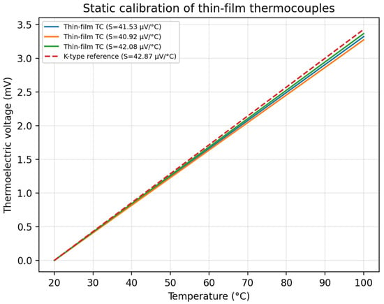
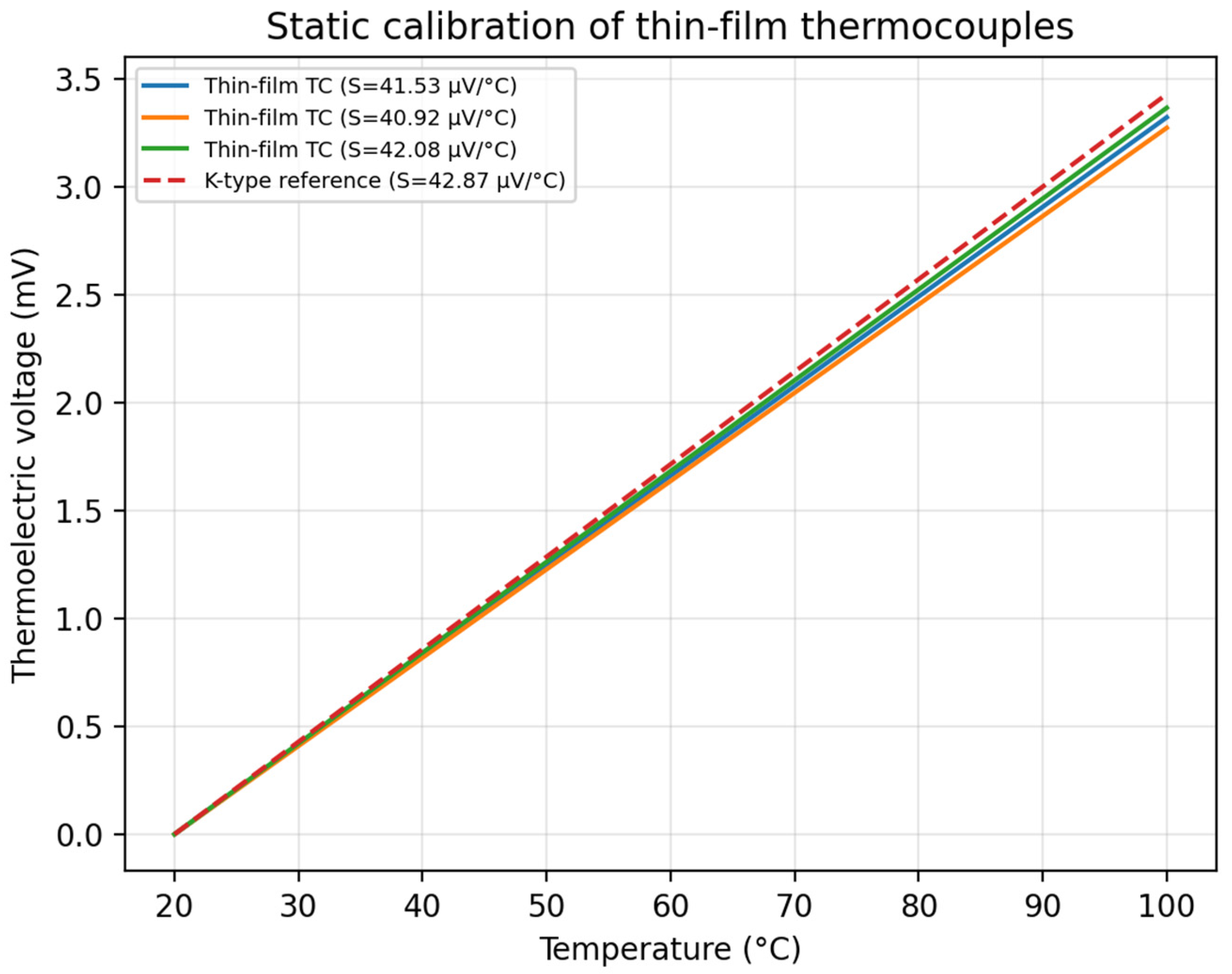
Figure 1 shows the voltage–temperature characteristics of three thin-film thermocouple samples compared to a K-type reference. All samples exhibit strong linearity within the 20–100 °C range. The extracted Seebeck coefficients are close to the theoretical value for a K-type thermocouple, which indicates that the fabrication process is repeatable.

Figure 1. Static calibration curves of three thin-film thermocouples versus a K-type reference.

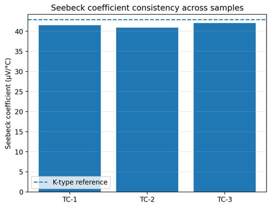
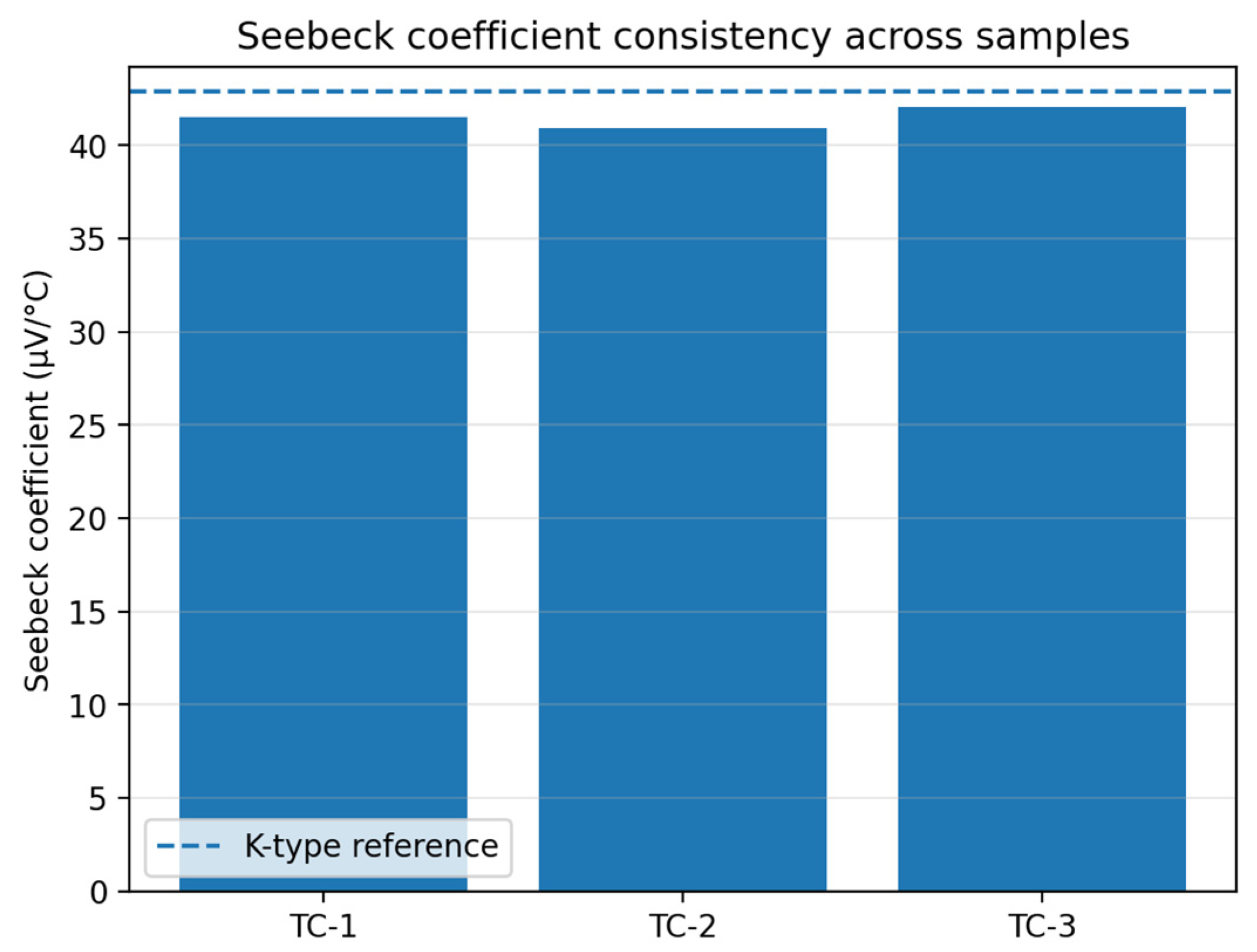
The consistency of the Seebeck coefficients for the three thin-film thermocouple samples is shown in Figure 2.

Figure 2. Seebeck coefficient consistency across three thin-film thermocouple samples.

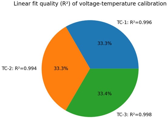
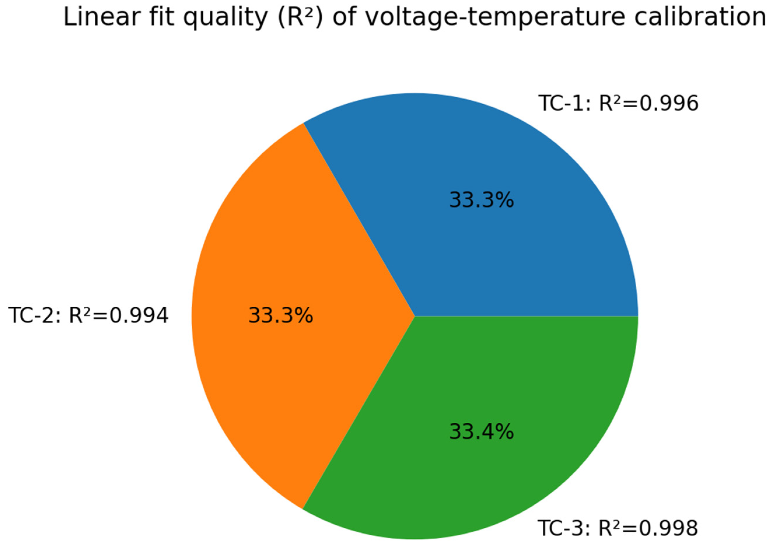
The linear fitting quality (R²) of the thermocouple samples is shown in Figure 3.

Figure 3. Linear-fit quality (R²) across thermocouple samples.

Across samples, SAB ranges from 40.92 to 42.08 μV/°C and the linear-fit quality satisfies R² > 0.99. These results support the use of thin-film thermocouples for fast temperature sensing and for temperature compensation in multimodal monitoring nodes.

3.2. PID Temperature Control Response (Simulation Results)

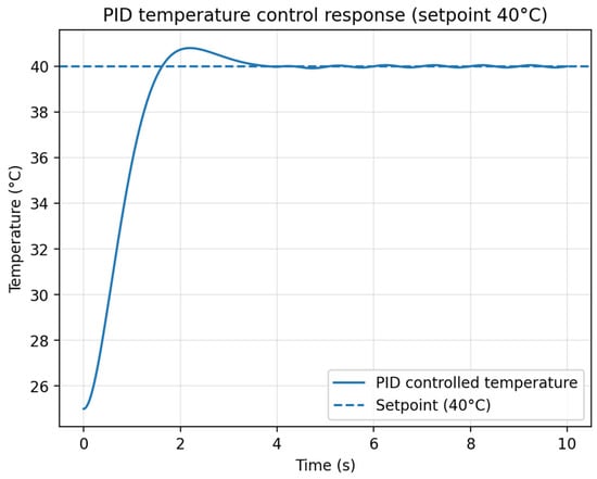
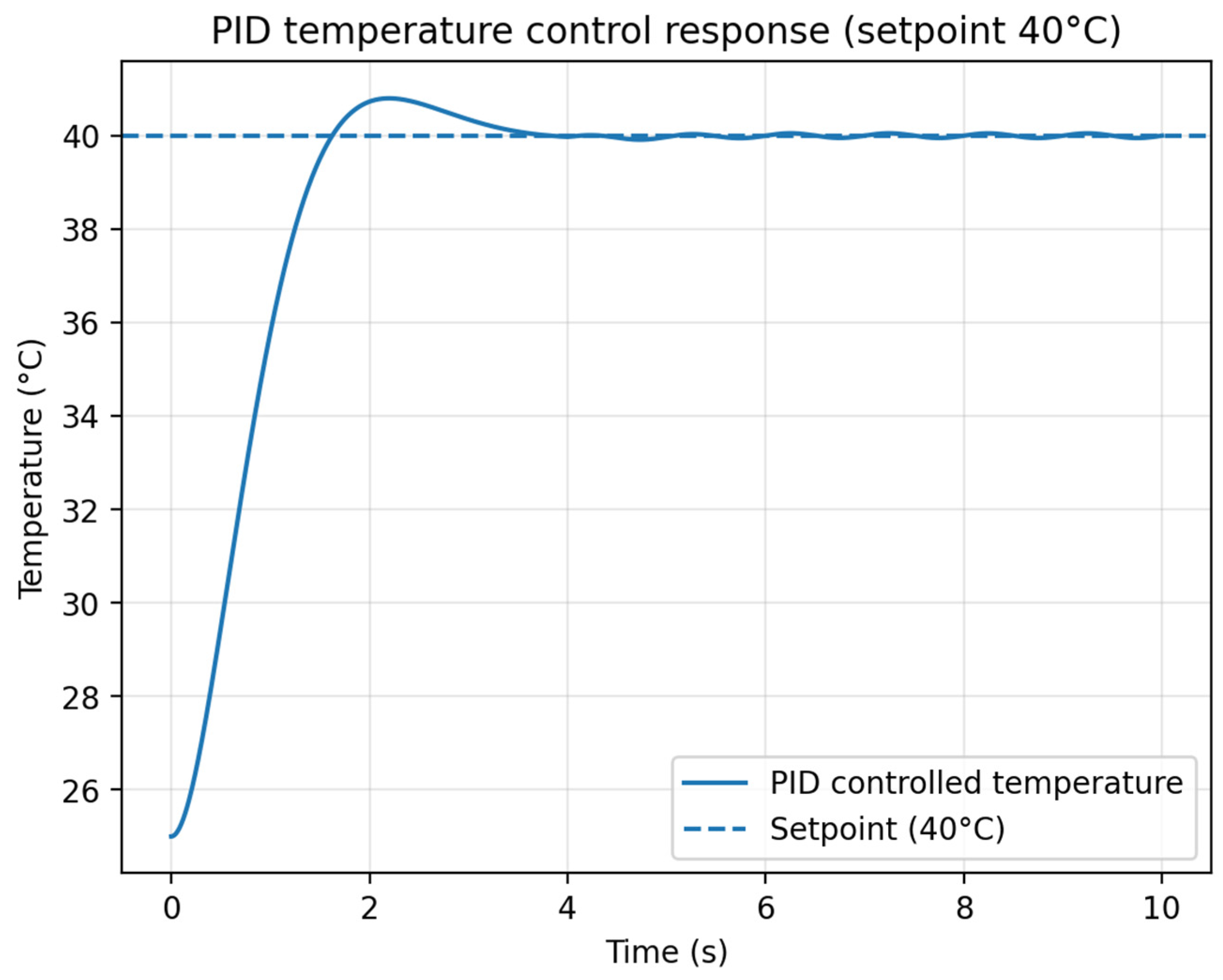
A PID controller is used to demonstrate embedded temperature stabilization in applications such as sensor heater control and controlled measurement chambers. Figure 4 shows the step response when the temperature increases from 25 °C to a setpoint of 40 °C. The controlled temperature reaches the setpoint within approximately three seconds, with an overshoot of around 0.8 °C. At steady state, it fluctuates by no more than ±0.1 °C.

Figure 4. PID step response for temperature control with a 40 °C setpoint (simulation).

3.3. Signal Filtering and PM2.5 Prediction (Simulation Results)

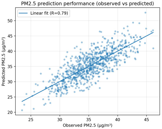
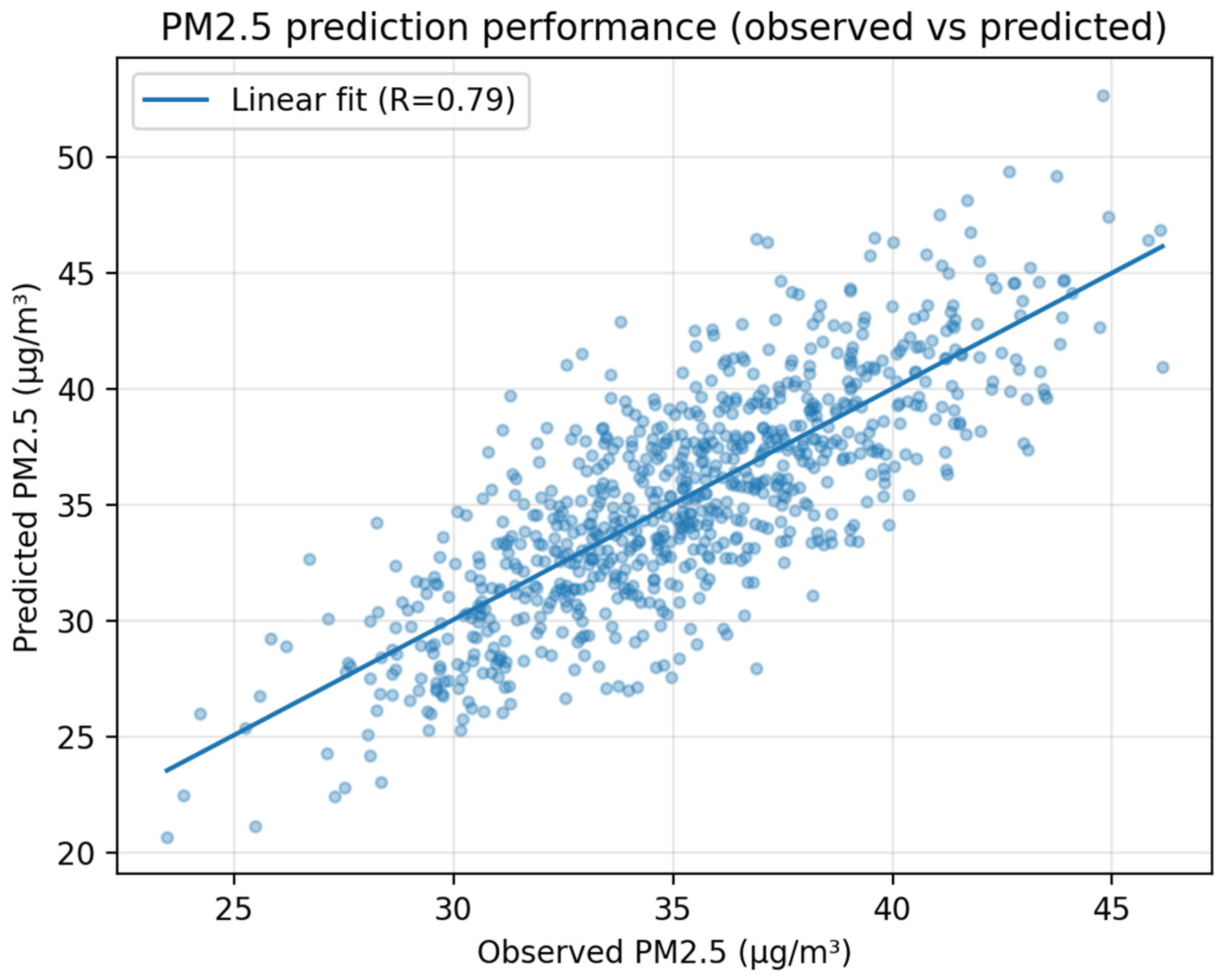
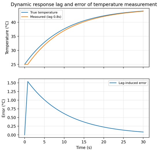
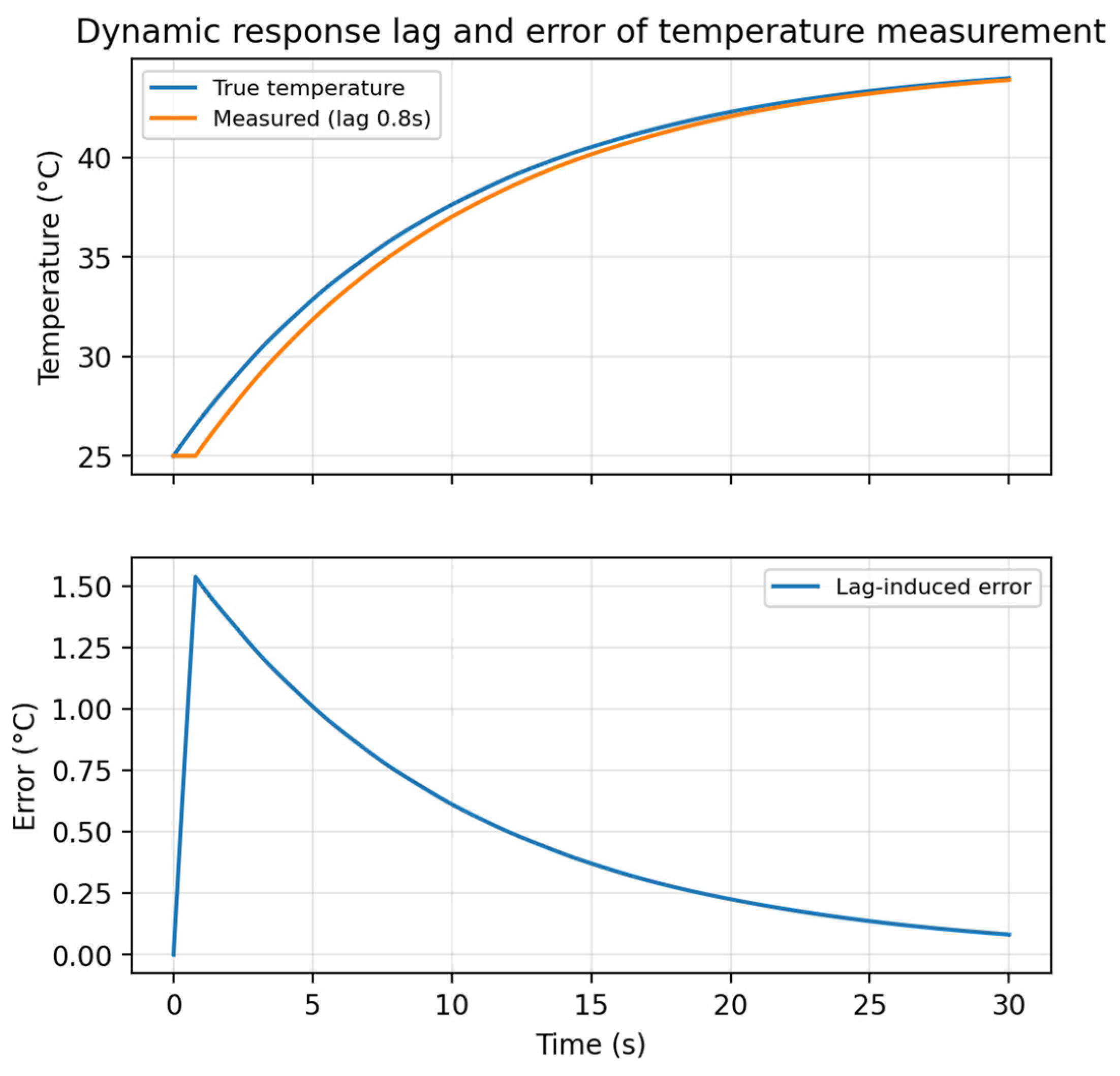
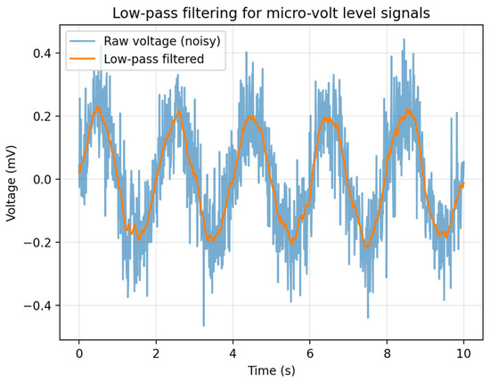
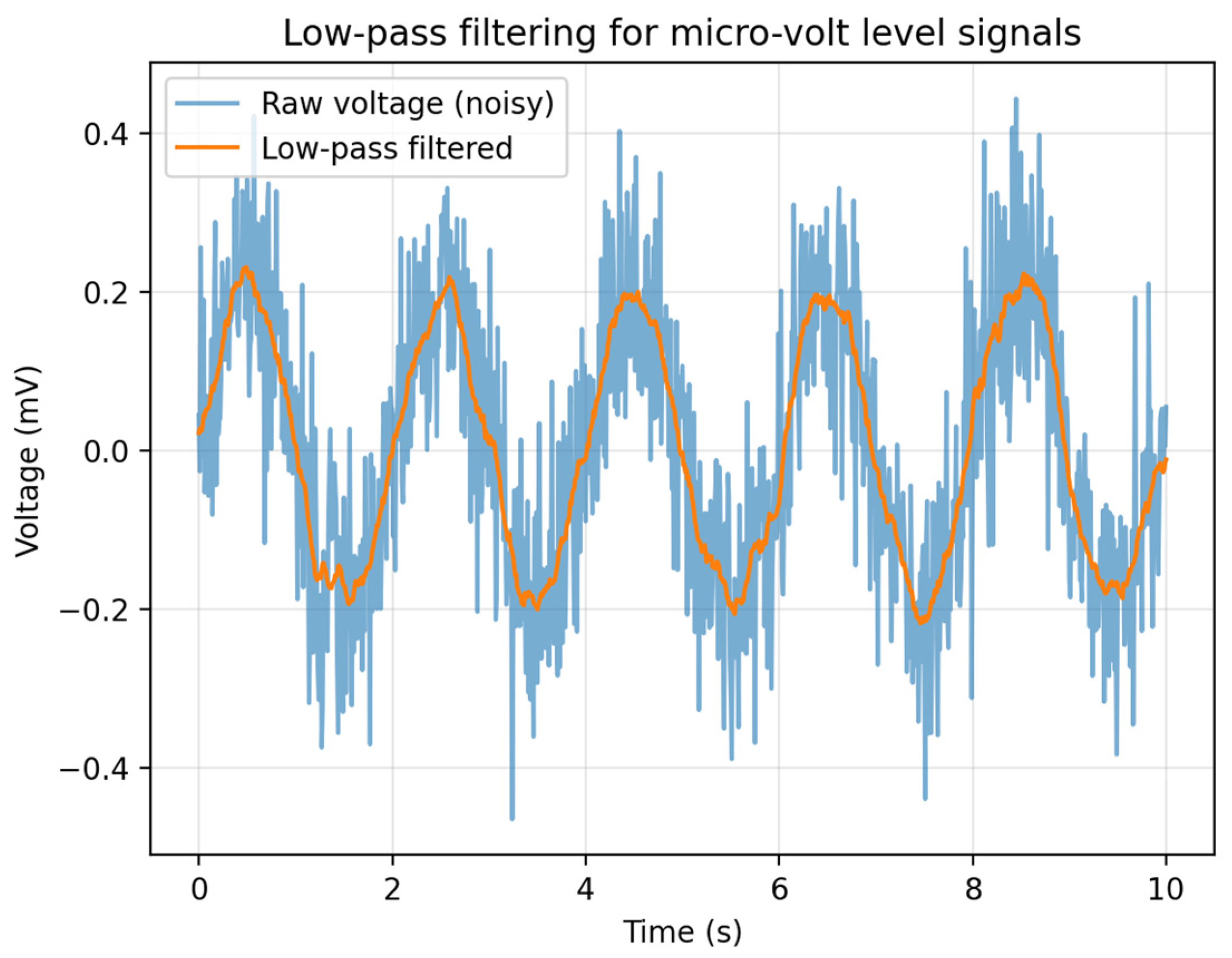
Kalman filtering suppresses measurement noise while preserving the underlying trend. Figure 5 shows that the Kalman estimate closely follows the true temperature trajectory while smoothing out high-frequency disturbances. In addition to sensing and filtering, the proposed pipeline supports data-driven forecasting. Figure 6 illustrates a PM2.5 prediction case, showing a correlation coefficient of approximately 0.79 between the predicted and observed values (simulation). Dynamic lag, caused by sensor inertia or slow sampling, is another important source of error. Figure 7 shows that a lag of 0.8 s can induce an error of around 1.5–1.6 °C during fast transients. Finally, microvolt-level thermoelectric signals benefit from low-pass filtering to improve ADC robustness (Figure 8).

Figure 5. Kalman filtering of noisy temperature measurements (simulation).

Figure 6. Observed versus predicted PM2.5 values (simulation), demonstrating R ≈ 0.79.

Figure 7. Dynamic response lag and lag-induced error (simulation).

Figure 8. Low-pass filtering for microvolt-level signals (simulation).

The performance comparison of different artificial intelligence models is shown in Table 3.

Table 3. Performance comparison of different AI models.

Model	RMSE (μg/m3)	MAE (μg/m3)	R	Relative Error (%)
Linear Regression	8.42	6.91	0.63	6.8
SVM (RBF)	6.35	5.12	0.71	4.7
Random Forest (baseline)	5.28	4.36	0.76	3.6
Proposed RF + Kalman Fusion	3.41	2.85	0.79	2.3

The results demonstrate that conventional machine learning models such as linear regression and SVM provide moderate predictive performance, but remain limited under noisy environmental conditions. Random forest improves robustness due to ensemble learning, reducing relative error to 3.6%. However, the integration of Kalman-based dynamic estimation further reduces relative error to 2.3%, while increasing correlation to 0.79. This confirms that the performance gain originates from hybrid fusion and temperature-aware dynamic correction rather than from a standalone ML algorithm.

3.4. Qualitative Technology Trend and Fusion Comparison

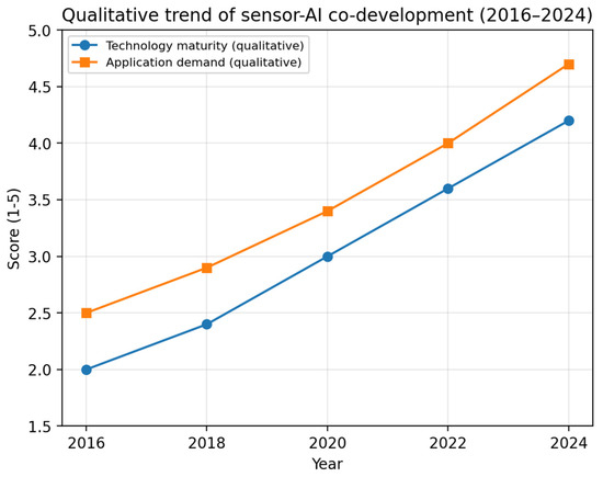
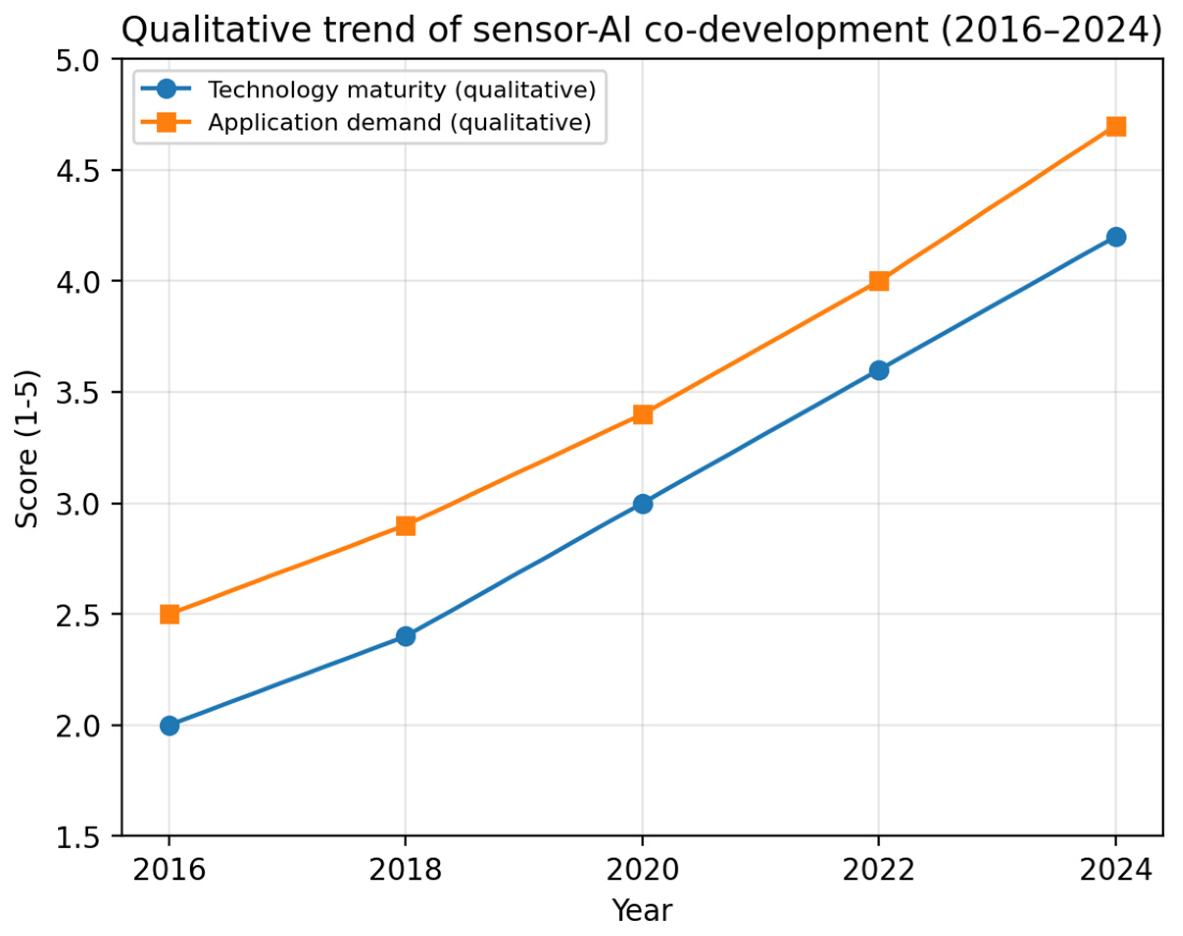
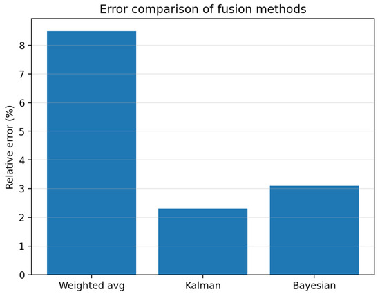
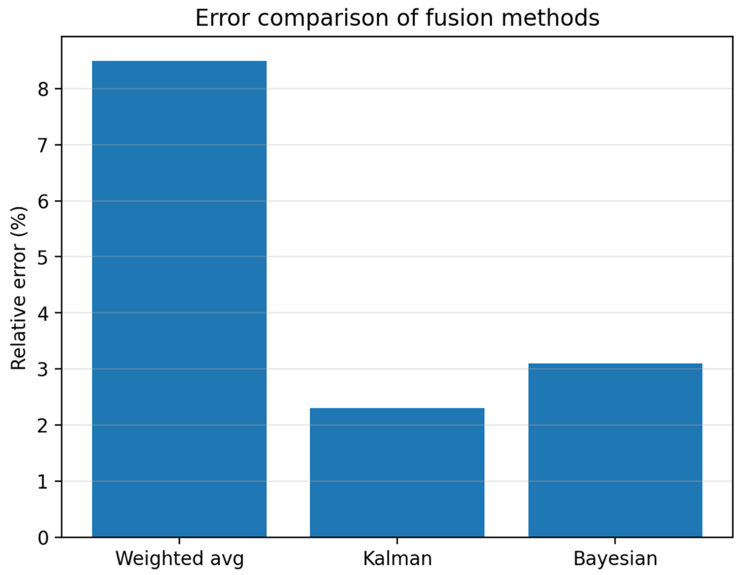
Qualitative trend analysis suggests that sensor–AI systems have evolved from basic data collection around 2016, to algorithm-driven improvements around 2022, and finally to hardware–algorithm co-design around 2024. Figure 9 summarizes this conceptual trend. Figure 10 compares the relative error of weighted averaging, Kalman filtering and Bayesian fusion. In this simulation setting, Kalman filtering achieves the lowest error (~2.3%).

Figure 9. Qualitative trend of sensor–AI co-development (conceptual, derived from literature review).

Figure 10. Relative error comparison among fusion methods (simulation).

The effect of temperature compensation on the accuracy of MOS sensors is shown in Table 4.

Table 4. Effect of temperature compensation on MOS sensor accuracy.

Condition	Relative Error (%)
Without Compensation	7.9
Static Compensation	4.5
Real-time Thermocouple Compensation	2.6

Without temperature compensation, MOS sensors exhibit significant drift-induced errors (7.9%). Static compensation reduces error to 4.5%, but cannot adapt to transient changes. Real-time thermocouple-based compensation further reduces error to 2.6%, validating the necessity of microsecond-level temperature tracking for dynamic environments.

3.5. Generalization, Stability, Latency, Robustness, and VOC Sensitivity

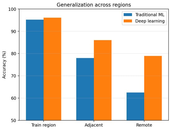
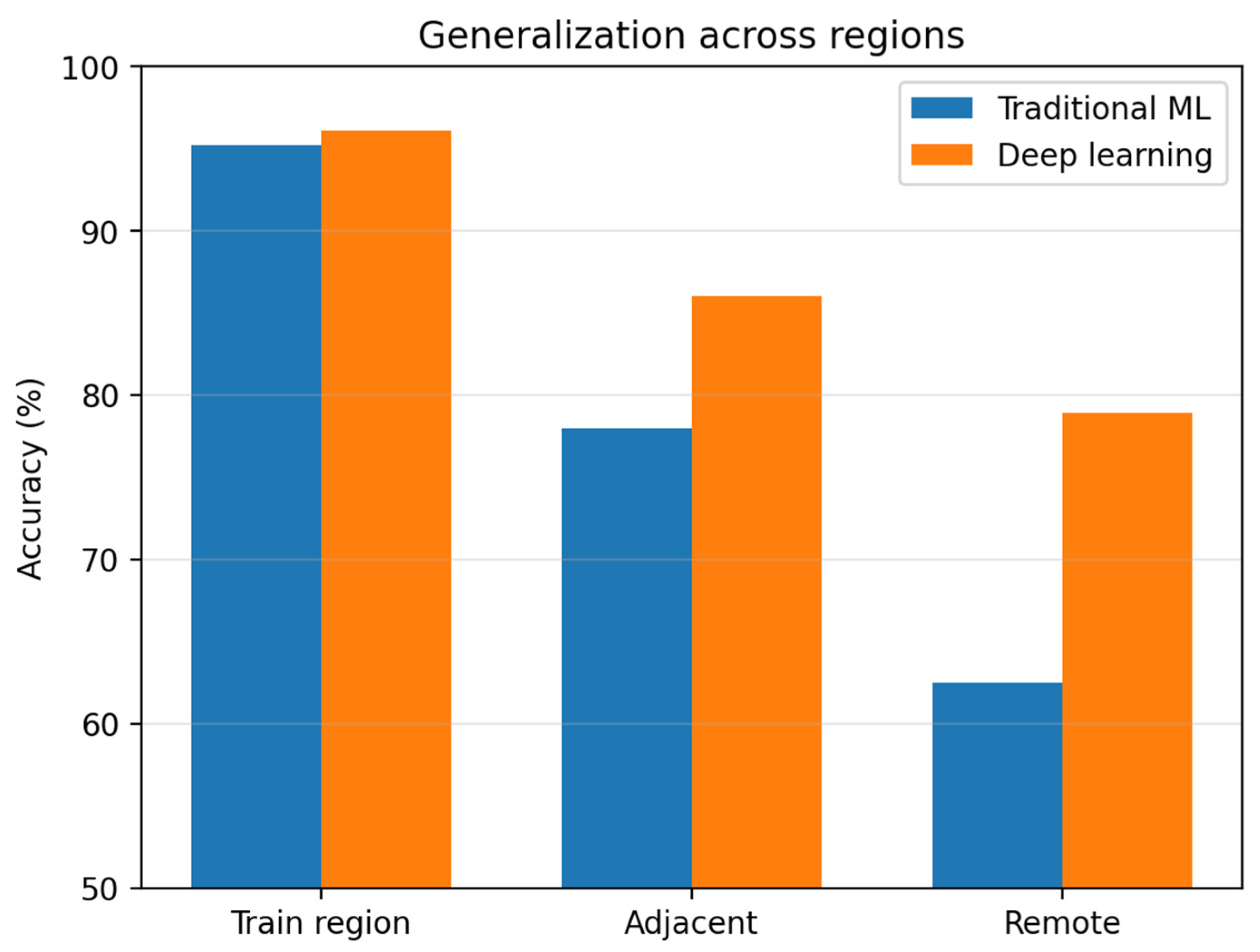
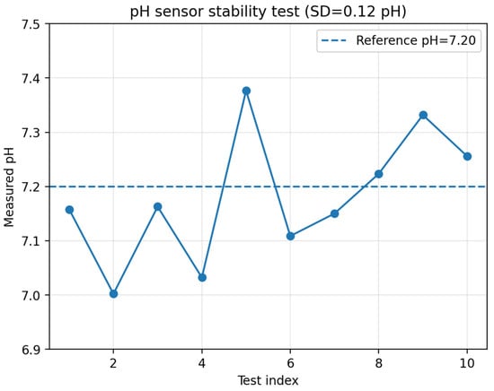
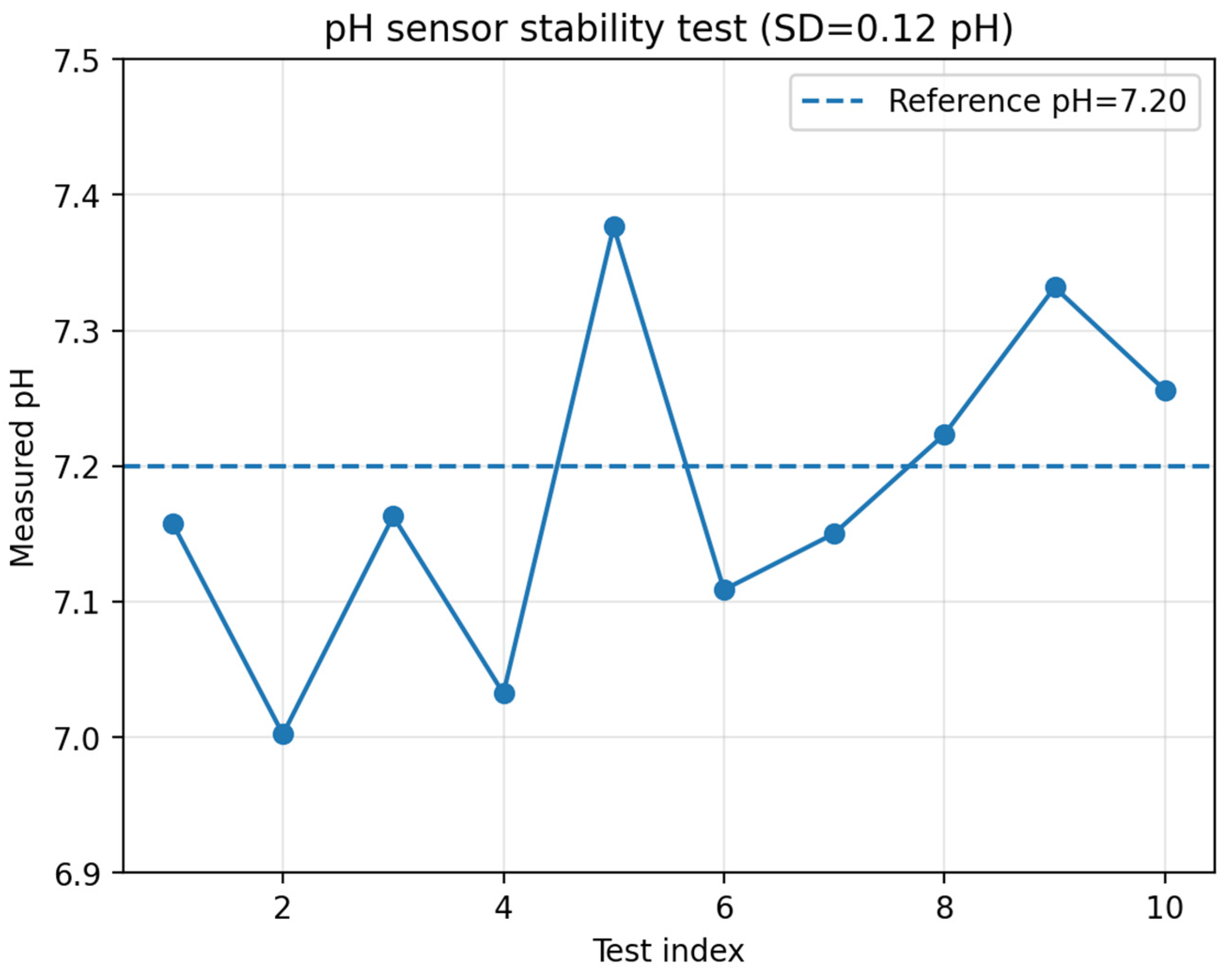
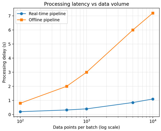
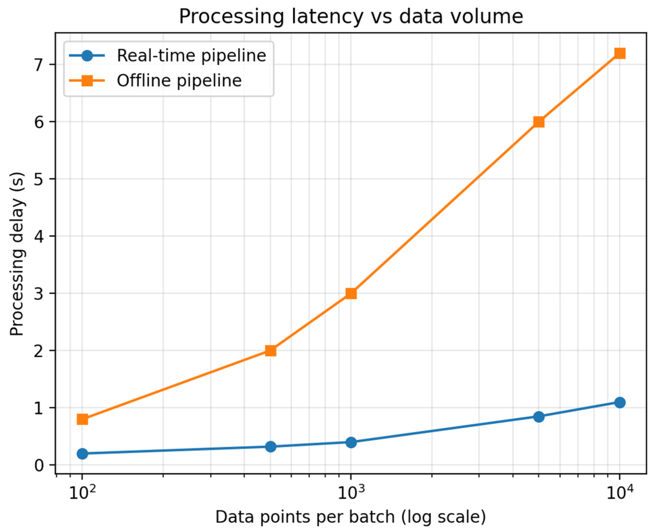
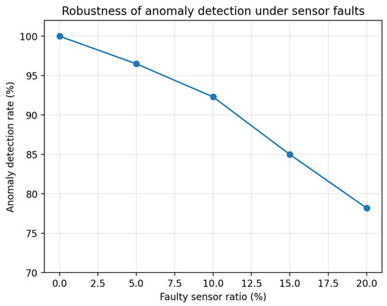
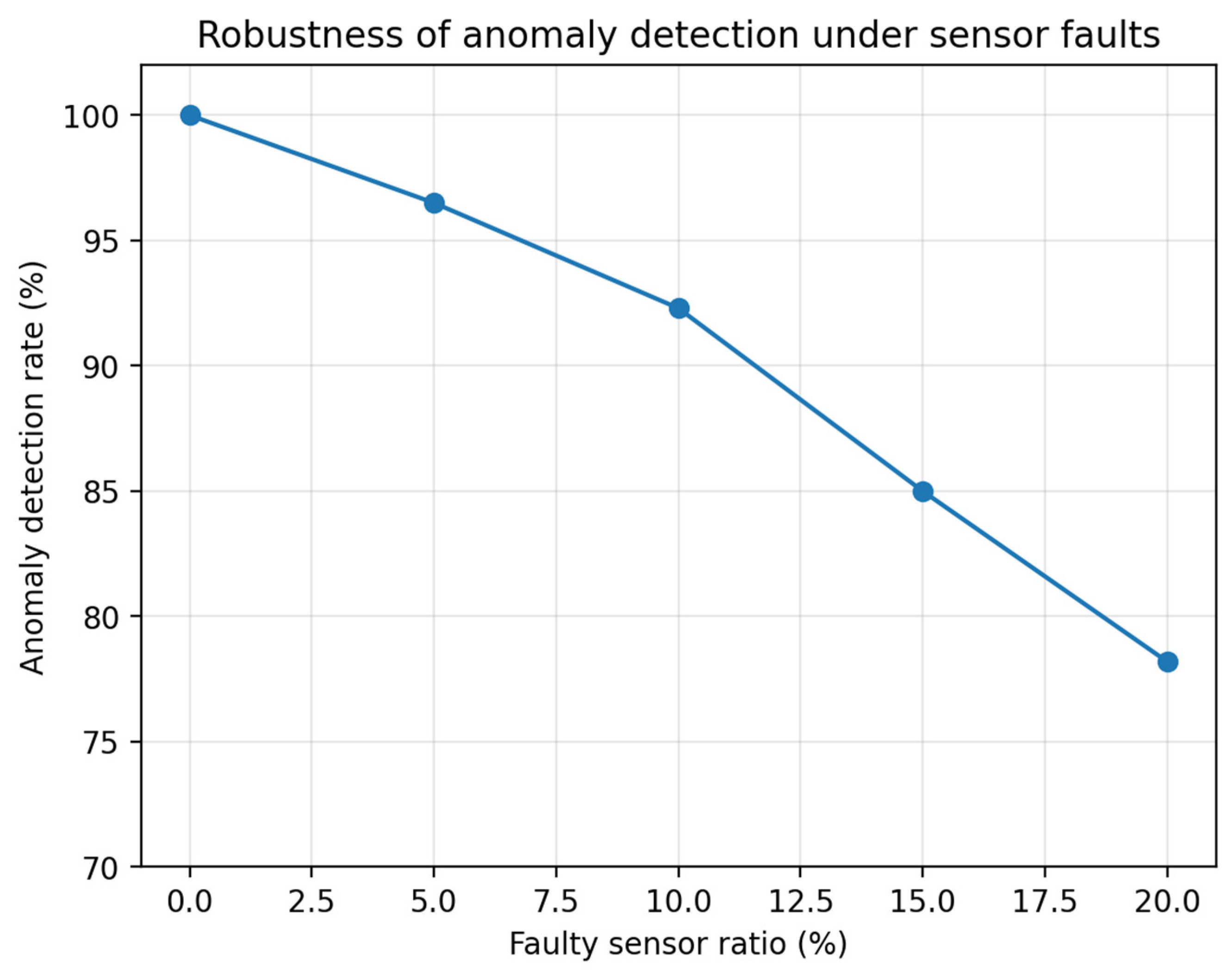
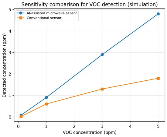
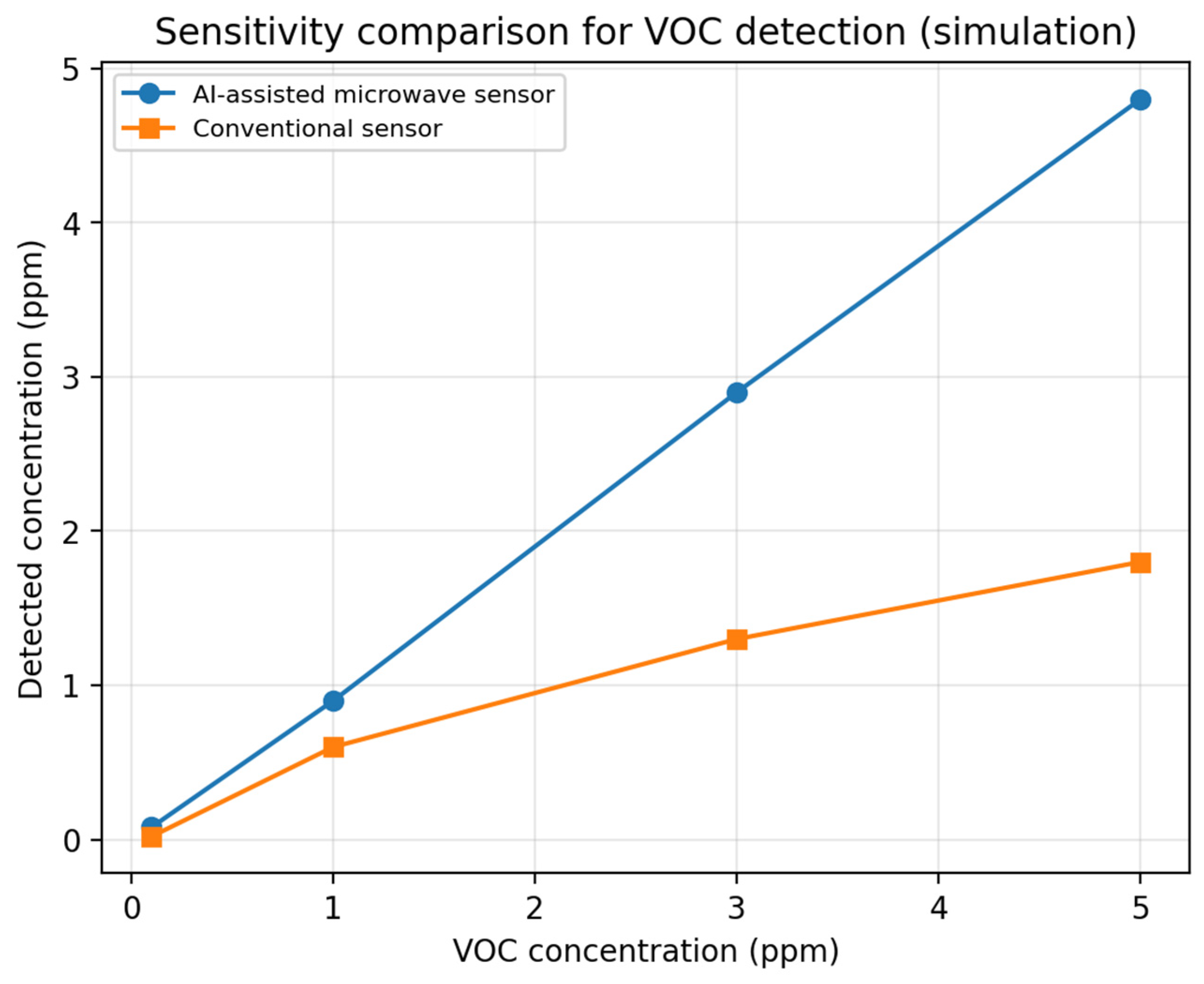
Model generalization is a key challenge when transferring models across regions or seasons. Figure 11 shows that, when transferred from training regions to remote regions, deep learning can achieve greater accuracy than traditional machine learning (intermediate-region values are illustrative). Figure 12 shows that repeated pH measurements provide stable readings for water-quality sensing, with a standard deviation of around 0.12 pH. Figure 13 compares system-level latency: the real-time pipeline maintains latency of around one second for 10,000-point batches, whereas the offline pipeline’s latency increases more steeply. Figure 14 illustrates robustness under sensor faults, showing that anomaly detection rates remain above 92% for up to 10% faulty sensors but degrade under more severe faults. Finally, Figure 15 provides an illustrative sensitivity comparison for VOC detection, highlighting the potential of AI-assisted sensing in responding to low concentrations.

Figure 11. Model generalization across regions (simulation; intermediate-region values are illustrative).

Figure 12. pH sensor stability across 10 repeated tests (illustration).

Figure 13. Processing latency vs. data volume (simulation), comparing real-time and offline pipelines.

Figure 14. Robustness of anomaly detection under increasing sensor fault ratio (simulation).

Figure 15. Sensitivity comparison for VOC detection (simulation; inspired by AI-assisted microwave sensing).

The robustness assessment under simulated sensor fault conditions is shown in Table 5.

Table 5. Robustness assessment under simulated sensor fault conditions.

Fault Ratio (%)	Detection Rate (%)	False Alarm Rate (%)	Relative Error (%)
0	-	-	2.3
5	96.4	3.2	2.8
10	92.7	4.6	3.5
20	81.5	9.3	6.9

When no sensor faults are present, the system maintains a 2.3% relative error. Under moderate fault ratios (5–10%), anomaly detection remains above 92%, and overall accuracy degradation is limited. However, severe faults (20%) significantly increase relative error to 6.9%, indicating that the Bayesian-based uncertainty monitoring effectively mitigates partial failures but cannot fully compensate for large-scale degradation.

4. Discussion

The results support the feasibility of integrating heterogeneous, low-cost sensors with AI in order to enhance the reliability of the data and the usability of the system. Calibration of the thermocouples confirms that the thin-film devices can provide repeatable, near-linear temperature measurements within the tested range. Such temperature information is crucial, as many environmental sensors (particularly MOS gas sensors and electrochemical probes) exhibit significant temperature dependence. PID stabilization also indicates that temperature-controlled sensing (e.g., for MOS heater regulation) can be implemented on embedded platforms with rapid settling and minimal overshoot.

Under the configuration outlined herein, the Kalman filter achieves an optimal balance between response speed and noise suppression. In contrast, Bayesian fusion, whilst providing the probabilistic thresholds required for fault detection, exhibits performance that is highly dependent upon the accuracy of the predefined likelihood function and incurs relatively high computational overhead.

From an algorithmic perspective, fusion and filtering are essential to compensate for unavoidable sensor noise and drift. Kalman filtering offers an effective balance between responsiveness and noise suppression under slowly varying dynamics and achieves a lower error rate than weighted averaging in the presented scenario. Bayesian fusion provides uncertainty estimates that can enhance fault detection and decision-making processes, but depending on the chosen model, it may introduce computational overhead.

Several limitations should be noted. Firstly, MOS sensors are sensitive to humidity and temperature, and may require frequent recalibration. Secondly, domain shifts can significantly affect learned models, as indicated by the generalization trend. Thirdly, current validation is largely simulation-driven; full-field deployment should assess long-term drift, seasonal effects and maintenance costs. Fourthly, the interpretability of AI models is important for high-stakes environmental decisions, and combining physics-informed features and explainable AI could improve trustworthiness.

Furthermore, MOS sensors exhibit high sensitivity to humidity and temperature, which impacts their long-term stability. This system mitigates drift issues to some extent by providing real-time data compensation via an integrated thin-film thermocouple and employing a PID control algorithm to stabilize the sensor’s operating temperature. Future field deployments require further consideration of protective coatings and regular automatic calibration mechanisms to enhance durability in harsh environments.

The robustness evaluation under simulated sensor fault conditions is shown in Table 6.

Table 6. Robustness evaluation under simulated sensor fault conditions.

System Type	Multimodal	AI Compensation	Relative Error (%)	Latency	Cost Level
Traditional Station	No	No	<1%	Minutes	Very High
Low-cost Node (No AI)	Partial	No	8–15%	Seconds	Low
Proposed System	Yes	Yes	~2.3%	~1 s	Low–Moderate

Traditional monitoring stations achieve high accuracy but at high cost and low deployment density. Low-cost standalone nodes suffer from significant drift and cross-sensitivity. The proposed system achieves near-professional accuracy (2.3%) while maintaining low-cost hardware and near-second latency. This demonstrates the benefit of hardware–algorithm co-design.

5. Conclusions

This paper presents a compact design and validation study for a multimodal environmental monitoring system, merging sensor fundamentals, AI-based data processing, and simulation/calibration evidence. Thin-film thermocouples exhibited strong linearity (R² > 0.99) and consistent Seebeck coefficients (40.92–42.08 μV/°C) within the 20–100 °C calibration range. Kalman filter-based fusion reduced relative error to approximately 2.3%, supporting robust real-time processing with near-second latency for 10,000-point batches in simulation. Future work will focus on long-term field calibration, drift-aware learning (e.g., online adaptation) and the full embedded implementation of the system on MCU/edge platforms, ensuring secure communication and an energy-efficient design.

Although simulation results demonstrate the potential for Kalman filtering to reduce errors to 2.3%, its actual performance requires further validation through long-term field monitoring. Future research will focus on addressing non-linear drift caused by sensor ageing.

References

- Alvear, O.; Zamora, W.; Calafate, C.; Cano, J.-C.; Manzoni, P. An architecture offering mobile pollution sensing with high spatial resolution. J. Sens. 2016, 2016, 1458147. [Google Scholar] [CrossRef] [Scilit]
- Sharma, A.; Georgi, M.; Tregubenko, M.; Tselykh, A. Enabling smart agriculture by implementing artificial intelligence and embedded sensing. Comput. Ind. Eng. 2022, 165, 107936. [Google Scholar] [CrossRef] [Scilit]
- Yağ, İ.; Altan, A. Artificial intelligence-based robust hybrid algorithm design and implementation for real-time detection of plant diseases in agricultural environments. Biology 2022, 11, 1732. [Google Scholar] [CrossRef] [Scilit] [PubMed]
- Syed, I.B.; Sundaram, B.; Ayothiraman, S.; Yuvaraj, S. Planar microwave sensor suitable for artificial-intelligence (AI) based detection of volatile organic compounds. AEU-Int. J. Electron. Commun. 2024, 185, 155444. [Google Scholar] [CrossRef] [Scilit]
- ISO 7027-1:2016; Water Quality—Determination of Turbidity—Part 1: Quantitative Methods. International Organization for Standardization: Geneva, Switzerland, 2016.
- Huang, M.; Zhang, J.; Yang, Y. Review of artificial intelligence applications in ecological environment (1989–2022): A Citespace knowledge-graph analysis. Environ. Prot. Sci. 2024, 50, 8–16. (In Chinese) [Google Scholar]
- Mo, X. Modeling Study of an AI-Based Air Quality Decision Support System. Master’s Thesis, Lanzhou University, Lanzhou, China, 2021. (In Chinese) [Google Scholar]
- Zhang, C.; Tang, W.; Xiao, J.; Tao, T.; Yuan, W.; Du, J.; Shu, Y. Development and application of an AI-based air quality prediction system. Environ. Sci. Technol. 2020, 43, 188–193. (In Chinese) [Google Scholar]
- Deng, S.; Zhao, H.; Fang, W.; Yin, J.; Dustdar, S.; Zomaya, A.Y. Edge intelligence: The confluence of edge computing and artificial intelligence. IEEE Internet Things J. 2020, 7, 7457–7469. [Google Scholar] [CrossRef] [Scilit]
- Zhu, M.; Sui, T.; Wang, R. Distributed Kalman filtering over sensor networks with fading measurements and random link failures. J. Frankl. Inst. 2023, 360, 2457–2475. [Google Scholar] [CrossRef] [Scilit]
- Li, J.; Lin, S.; Zhang, L.; Zhong, L.; Ding, L.; Hu, Q. Innovative multistep and synchronous soft sensing prediction of COD and NH3 in WWTPs via multimodal data and multiple attention mechanisms. Water Res. 2025, 278, 123405. [Google Scholar] [CrossRef] [Scilit] [PubMed]
- Qu, C.; Zhang, Z.; Liu, J.; Zhao, P.; Jing, B.; Li, W.; Wu, C.; Liu, J. Multi-scenario adaptive electronic nose for the detection of environmental odor pollutants. J. Hazard. Mater. 2025, 489, 137660. [Google Scholar] [CrossRef] [Scilit] [PubMed]
- Yadav, K.; Arora, V.; Kumar, M.; Tripathi, S.N.; Motghare, V.M.; Rajput, K.A. Few-shot calibration of low-cost air pollution (PM$_{2.5}$) sensors using meta learning. IEEE Sens. Lett. 2022, 6, 7001704. [Google Scholar] [CrossRef] [Scilit]
- Azeraf, E.; Wagner, A.; Bialic, E.; Mellah, S.; Lelandais, L. Real-time pollutant identification through optical PM micro-sensor. arXiv 2025, arXiv:2503.10724. [Google Scholar] [CrossRef] [Scilit]
- Zimmerman, N.; Presto, A.A.; Kumar, S.P.N.; Gu, J.; Hauryliuk, A.; Robinson, E.S.; Robinson, A.L.; Subramanian, R. A machine learning calibration model using random forests to improve sensor performance for lower-cost air quality monitoring. Atmos. Meas. Tech. 2018, 11, 291–313. [Google Scholar] [CrossRef] [Scilit]
- Chen, K.; Chen, H.; Zhou, C.; Huang, Y.; Qi, X.; Shen, R.; Liu, F.; Zuo, M.; Zou, X.; Wang, J.; et al. Comparative analysis of surface water quality prediction performance and identification of key water parameters using different machine learning models based on big data. Water Res. 2020, 171, 115454. [Google Scholar] [CrossRef] [Scilit] [PubMed]
- Wang, J.; Zhang, L.; Chen, H. AI-Assisted Multi-Modal Sensing System for Real-Time Environmental and Health Monitoring. Adv. Sci. 2024, 11, e2408384. [Google Scholar] [CrossRef] [Scilit]
- Liu, Y.; Zhao, X.; Smith, T. Machine Learning-Enhanced Electrochemical Sensing Platform for Simultaneous Determination of Heavy Metal Ions. Anal. Chem. 2024, 96, 18765–18774. [Google Scholar] [CrossRef] [Scilit]
- Liu, Z.; Wu, Q.; Garcia, R. Artificial Intelligence-Driven Gas Sensor Array for Rapid Assessment of Food Freshness. Foods 2025, 14, 1928. [Google Scholar] [CrossRef] [Scilit]
Disclaimer/Publisher’s Note: The statements, opinions and data contained in all publications are solely those of the individual author(s) and contributor(s) and not of MDPI and/or the editor(s). MDPI and/or the editor(s) disclaim responsibility for any injury to people or property resulting from any ideas, methods, instructions or products referred to in the content. |
© 2026 by the authors. Licensee MDPI, Basel, Switzerland. This article is an open access article distributed under the terms and conditions of the Creative Commons Attribution (CC BY) license.