Switched-Inductor DC–DC Converters: Direct Small-Signal Equivalent AC Circuit

Abstract

Switched-inductor converters are ubiquitous in modern electronics. Their switching behavior makes them inherently nonlinear and unsuitable for classical linear frequency-response models, requiring linearization for stability analysis. Common approaches—such as state-space averaging, circuit averaging, and signal-flow graphs—can be algebraically intensive and may offer limited circuit-level interpretability. This paper proposes a direct small-signal AC response model for switched inductors in both CCM and DCM that preserves circuit intuition while maintaining the accuracy of conventional methods. The proposed framework enables the systematic derivation of the duty-cycle-to-output-voltage, duty-cycle-to-output-current, and duty-cycle-to-inductor-current transfer functions within a unified circuit representation. Bode plots of the duty-cycle-to-voltage and duty-cycle-to-current gains confirm that the model accurately captures the LC double pole and associated zeros, including the shift of the load-related zero in the reconstructed inductor-current gain. The resulting model remains straightforward to use, analyze, and simulate and may facilitate control-loop design as well as integration into automated synthesis or optimization tools. In DCM, the model further provides an analytical expression for the duty-cycle-to-inductor-current gain, contributing to a clearer understanding of this relationship in the literature. Results validated in SIMPLIS show excellent agreement with state-space averaging predictions.

1. Modeling the AC Dynamics of Switched Inductors

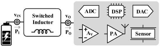
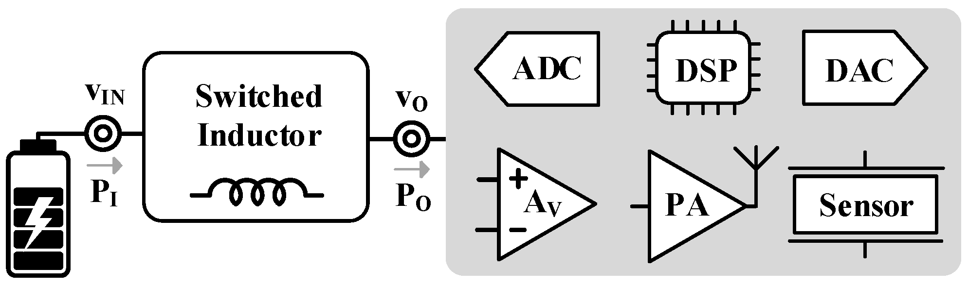
Switched-inductor converters rely on one or more negative feedback loops to regulate their output in response to variations in input voltage (e.g., from a battery) and/or load current (due to diverse load conditions [1], as shown in Figure 1). Modelling their AC dynamics is therefore essential for ensuring stability [2]. Three primary modelling approaches are used: state-space averaging (SSA), circuit averaging, and signal flow graphs [3,4,5,6,7,8,9,10,11].

Figure 1. Electronic system with power supply and load.

Switched-inductor converters alternate between states, each defined by differential equations for current and voltage. Averaging these over a constant switching period t_SW enables small-signal analysis [3,4,5]. SSA also supports matrix representations, which, when combined with digital control, facilitate advanced control techniques [12,13,14,15]. However, modeling linear subcircuits can be algebraically intensive, as this approach requires decomposing each variable into its DC and perturbation components and neglecting higher-order perturbation products for every variable, which can obscure the physical origins of the resulting poles and zeros. Additionally, in DCM, studies [3,4] require the switching period to be divided into three subintervals, with separate sets of equations describing each state; thus, the approach relies on multiple piecewise equations.

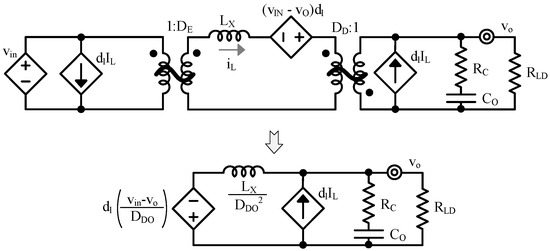
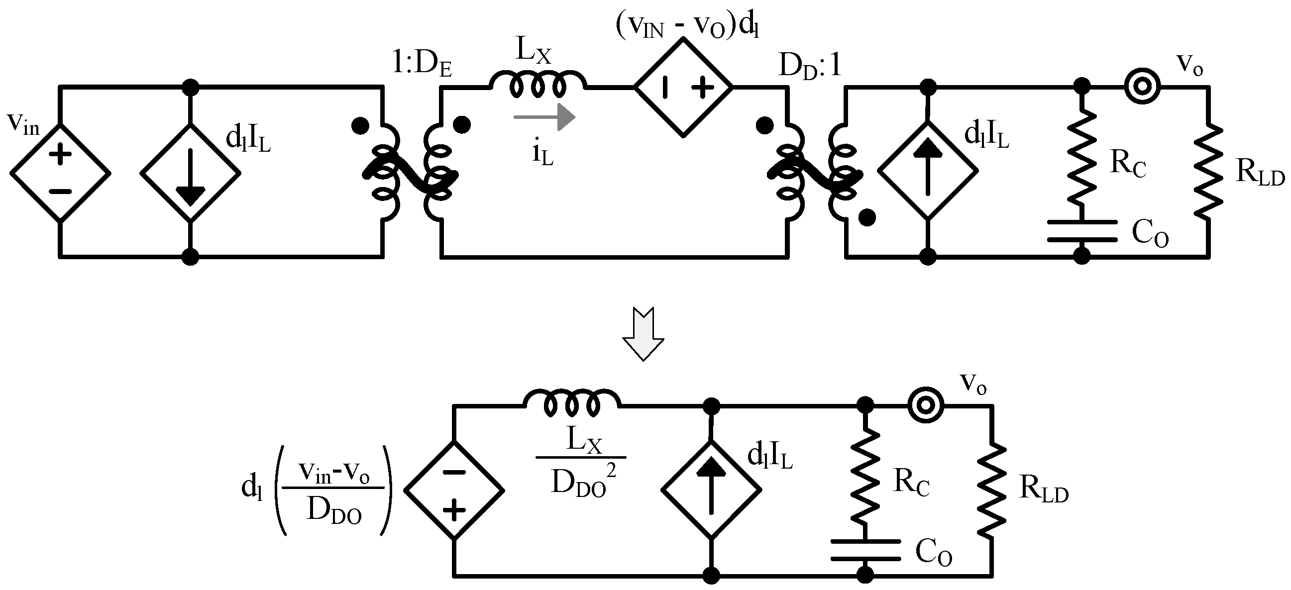
Circuit averaging replaces nonlinear subcircuits with ideal transformers and dependent sources [6,7,8]. These equivalent circuits are derived from SSA-based equations and often provide more intuitive insight. However, the method shares SSA’s mathematical complexity and limitations. Namely, a buck–boost circuit (for instance) must first be converted into its equivalent circuit averaged form, where the switches are replaced by ideal transformers, as illustrated in Figure 2. Additional manipulations are then required to push the inductor and voltage through the transformer, derive the control-to-output transfer function, and superpose the two contributions from the control-signal-dependent current and voltage sources. The inverting zero subsequently appears in the transfer function, but its origin is obscured by all the intermediate steps needed to obtain the equivalent circuit.

Figure 2. Buck–boost circuit SSA equivalent form.

Flow graphs convert SSA equations into visual representations using nodes and branches, where each branch corresponds to a small-signal transfer function [9,10,11]. This method decomposes the overall AC response into identifiable gain stages and does not require several rounds of transformations to obtain its final form. However, as described in [16], the signal flow graph does not resemble a circuit, offering very little insight into the physical meaning of the different sub-transfer functions.

This work presents a new method for modeling the AC response of switched inductors, based entirely on circuit representation. Like signal flow graphs, it derives the transfer function of each component averaged over t_SW. Unlike SSA, it avoids algebraic manipulation and transformer-based modeling to obtain the gains. The method yields equivalent Norton and Thevenin circuits for the switched inductor and its driving network. As with SSA, circuit averaging, and flow-graph approaches, it captures the AC response of converters operating under constant switching-frequency PWM but in the form of a circuit. Specifically, it models the converter’s small-signal response to variations in the duty-cycle command d_L. The model presented in this work is straightforward to use, analyze, and simulate, making it suitable for practical implementation and design studies. Being able to rapidly derive the small-signal gains of a switched inductor without going through multiple translation steps saves significant design time. It is important to note that the model is valid for small perturbations around the operating point and constant-frequency operation; effects such as current-mode control strategies, variable-frequency operation, or switching nonlinearities are out of scope and are not captured by this approach.

The proposed modeling procedure requires the following inputs: the converter topology, the switching intervals for each active switch (energizing and draining duty cycles values), and the relevant circuit variables such as inductance, output capacitor, and load and parasitic resistances. From these inputs, the method produces circuit-level equivalents, such as Norton or Thevenin representations of the converter, along with the key small-signal transfer functions describing the control-to-output voltage, control-to-output current, and control-to-inductor current dynamics. This formalization makes the approach directly verifiable: given a converter and its switching pattern, one can reproduce the equivalent circuits and extract the same transfer functions, ensuring reproducibility and transparency in the analysis.

This paper is structured as follows: Section 2 introduces basic switched inductor circuits and small signal models, Section 3 presents the model and its validation in Continuous-Conduction Mode (CCM), while Section 4 covers the Discontinuous-Conduction Mode (DCM) and its validation. Section 5 concludes this article. Throughout this paper, the notation s_A represents both large- and small-signal quantities, whereas S_A and s_a refer to large-signal and small-signal components, respectively.

2. Switched-Inductor DC–DC

2.1. Variants

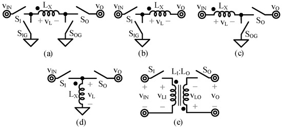
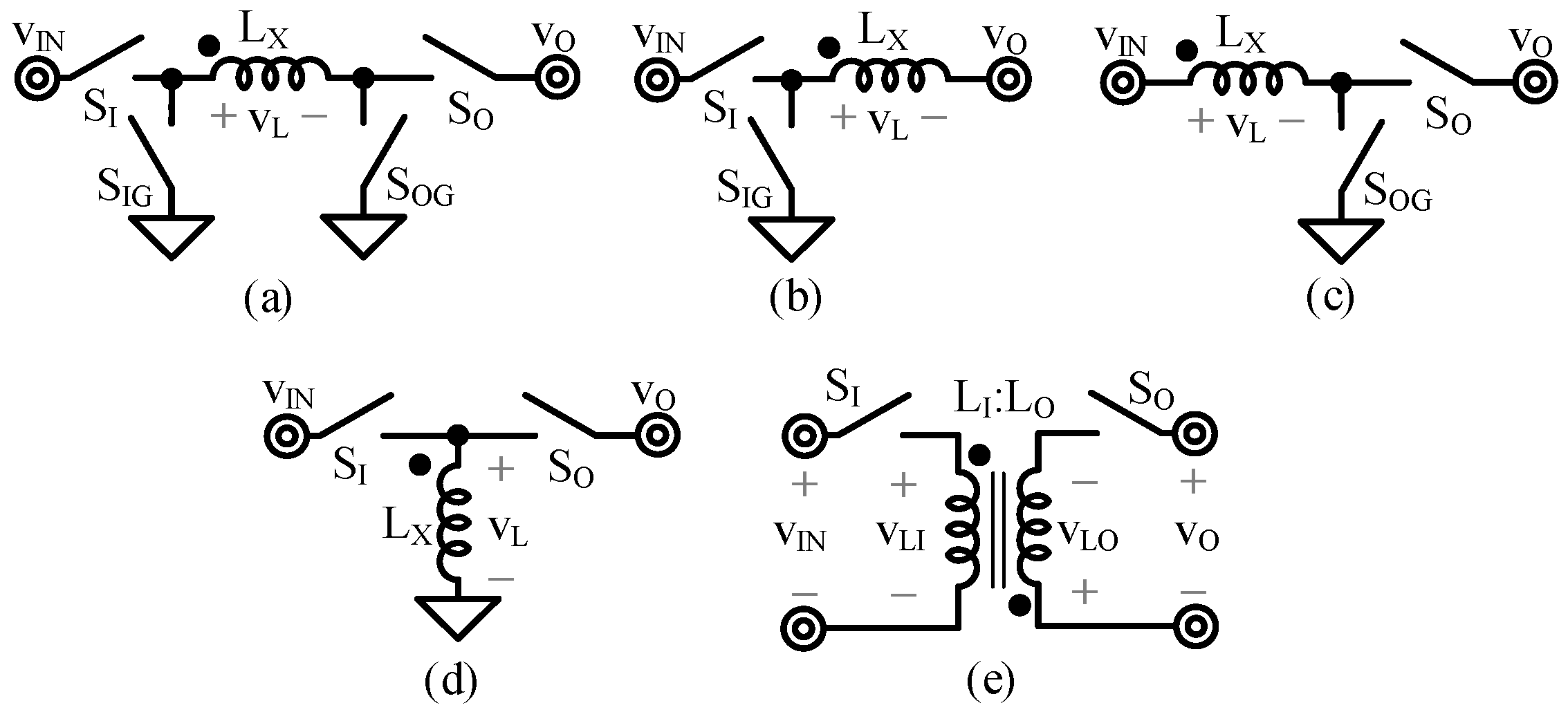
Switched-inductor converters use an inductor L_X as an intermediate energy storage element. The inductor is first energized (during an energizing duty cycle fraction d_E of t_SW) from the input voltage v_IN, and then its stored energy is drained to the output v_O. Five classical topologies include buck (v_IN > v_O), boost (v_IN < v_O), buck–boost (v_IN> or <v_O), inverting buck–boost (v_IN > 0 > v_O), and flyback (v_IN> or <v_O and isolated input and output grounds), as Figure 3 shows. The flyback converter employs a transformer with an input winding denoted as L_I and an output winding denoted as L_O. The transformer has a turns ratio k_L. On the primary (input) side, the inductor voltage and current are v_LI and i_LI, and on the secondary (output) side they are v_LO and i_LO. The currents i_LI and i_LO together form the transformer current i_XO (i_LI/k_L + i_LO) as referred to the output side. The buck–boost topology typically uses four switches, whereas the buck converter uses two input-side switches (S_I and S_IG) and the boost converter uses two output-side switches (S_O and S_OG).

Figure 3. Switched-inductor variants: buck–boost (a), buck (b), boost (c), inverting buck–boost (d), and flyback (e).

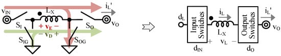
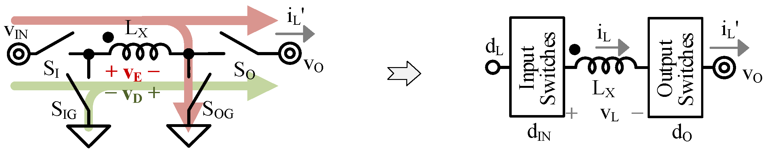
In all these configurations, the switched inductor can be represented as a network of switches connecting the inductor L_X to v_IN, v_O, and ground, as Figure 4 illustrates. d_O and d_D denote the fractions of t_SW during which L_X connects to v_O, and during which it is draining, respectively. When S_O is present, it duty-cycles L_X into v_O, so d_O is d_D. When there is no S_O, d_O is 1. For boost-derived variants, since L_X does not always connect to v_O, the inductor current i_L is a duty cycle d_O fraction of the power stage output current i_L′. It is important to note that the duty cycles are defined only for the intervals when the inductor is conducting current. The dot on the inductor indicates the positive terminal. When a positive voltage is applied across the inductor relative to this dot, the inductor energizes, whereas applying a negative voltage causes it to drain. Table 1 summarizes the voltages, duty cycles, and output currents for the different converter variants. In this work, the voltage causing the inductor to discharge is treated as a positive quantity, as it is applied with reverse polarity relative to the dot, as illustrated in Figure 4.

Figure 4. General topology of switched-inductor converters.

Table 1. Voltages and duty cycles for switched inductor variants.

Topology	vE	vD	dE	dD = 1 − dE	dO	iL′
Buck–boost	vIN	vO	${\displaystyle \frac{v_{IN}}{{v_{IN}+v}_O}}$	${\displaystyle \frac{v_O}{{v_{IN}+v}_O}}$	dD	$d_O{i}_L$
Inverting buck–boost	vIN	−vO	${\displaystyle \frac{\left|v_O\right|}{v_{IN}+\left|v_O\right|}}$	${\displaystyle \frac{v_{IN}}{v_{IN}+\left|v_O\right|}}$	dD	$d_O{i}_L$
Buck	vIN − vO	vO	${\displaystyle \frac{v_{IN}}{v_O}}$	${\displaystyle \frac{{v_O-v}_{IN}}{v_O}}$	1	iL
Boost	vIN	vO − vIN	${\displaystyle \frac{{v_O-v}_{IN}}{v_O}}$	${\displaystyle \frac{v_{IN}}{v_O}}$	dD	$d_O{i}_L$
Flyback	vIN	vO	${\displaystyle \frac{v_O}{{v_{IN}{k}_L+v}_O}}$	${\displaystyle \frac{v_{IN}{k}_L}{{v_{IN}{k}_L+v}_O}}$	dD	$d_O{i}_{XO}$

2.2. Continuous-Conduction Mode

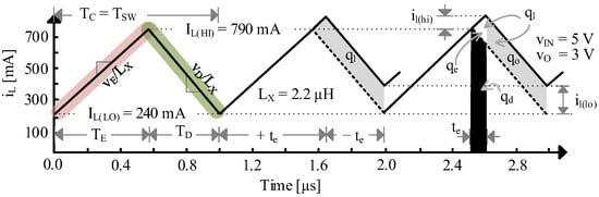
During the energizing phase, the voltage v_L applied across L_X is the energizing voltage v_E, which causes i_L to rise to its peak value, i_L(HI). In the subsequent draining phase, a draining voltage v_D is applied across L_X in the opposite direction. Both v_E and v_D include the effects of ohmic voltage drops due to parasitic resistances. This results in i_L decreasing by the same amount, Δi_L, as Figure 5 illustrates.

Figure 5. i_L in CCM and small signal variation (buck, 515 mA load, simulated with LTSpice).

At the end of the draining time t_D, a new energizing phase begins. The inductor current i_L reaches its minimum value, i_L(LO), at the end of the draining phase. When this value is greater than or equal to zero without a zero-current interval, the converter operates in CCM. In this mode, the conduction time t_C equals the full switching period t_SW, and the energizing time t_E is a d_E fraction (the energizing duty cycle) of t_C. In this case, the duty cycle command d_L, which controls the switches, is equal to d_E. Equation (1) below defines Δi_L:

$${∆i}_L=i_{L\left(HI\right)}-i_{L\left(LO\right)}=\left({\displaystyle \frac{v_E}{L_X}}\right)d_E{t}_{SW}.$$

(1)

d_L is the effective control signal governing the power switches, while d_E and d_D denote the fractions of the conduction interval during which the inductor energizes and discharges, respectively. In continuous conduction mode (CCM), d_E is active during the interval in which the inductor is energizing.

2.3. Discontinuous-Conduction Model

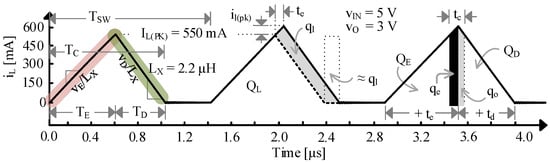
When i_L(LO) is zero and the current remains at zero for a finite interval, the converter operates in DCM. In this mode, i_L rises during the energizing phase with v_E and falls during the draining phase with v_D. It then remains at zero until the next switching cycle begins. This causes t_C to be effectively shorter than t_SW, as Figure 6 below illustrates. As a consequence, T_E and T_D are d_ET_C and d_DT_C, respectively.

Figure 6. i_L in DCM and small signal variation (buck, 200 mA load, simulated with LTSpice).

Under these conditions, d_E no longer represents the ratio t_E/t_SW that the duty cycle command d_L would typically control. This is because, in addition to the energizing and discharging intervals, a third time interval exists which, together with the conduction intervals, completes the switching period. In DCM, the peak inductor current is denoted as i_L(PK):

$$i_{L\left(PK\right)}=\left({\displaystyle \frac{v_E}{L_X}}\right)d_E{t}_C.$$

(2)

2.4. Small-Signal Model

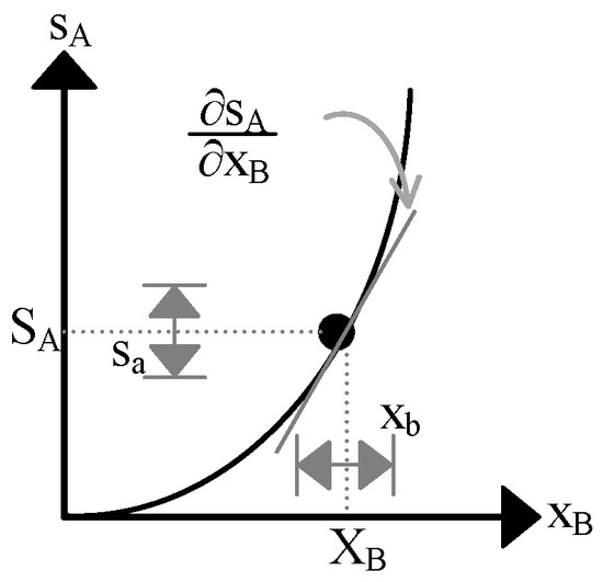
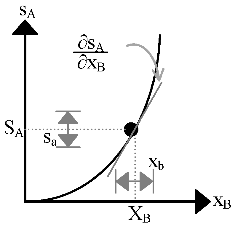
The way regulated systems respond to disturbances depends on small-signal behavior. Fortunately, feedback significantly reduces these variations, allowing linear approximations to model them accurately. For instance, in Figure 7, the linear region of the exponential-like response can translate small changes in the input signal x_B to the output signal s_A with results that closely match the true variations of s_A. The small-signal component x_b in x_B represents slight deviations around the static point X_B; the local slope (partial derivative) of s_A with respect to x_B at that point determines how these input perturbations produce corresponding small-signal responses s_a in s_A:

$$s_a\approx x_b\left({\displaystyle \frac{\partial s_A}{\partial x_B}}\right).$$

(3)

Figure 7. Linear projection of small-signal variation.

In modern power supplies, d_L is connected to the gates of CMOS transistors, as Figure 8 shows. Since these gates exhibit capacitive behavior and are largely unaffected by the network dynamics, d_L primarily interacts with the gate capacitance C_G. Consequently, the small-signal model that includes this C_G does not incorporate any feedback-related effects.

Figure 8. Small-signal translations.

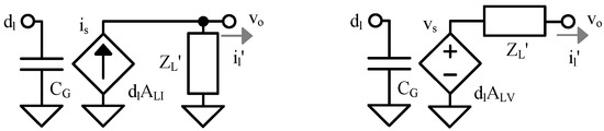
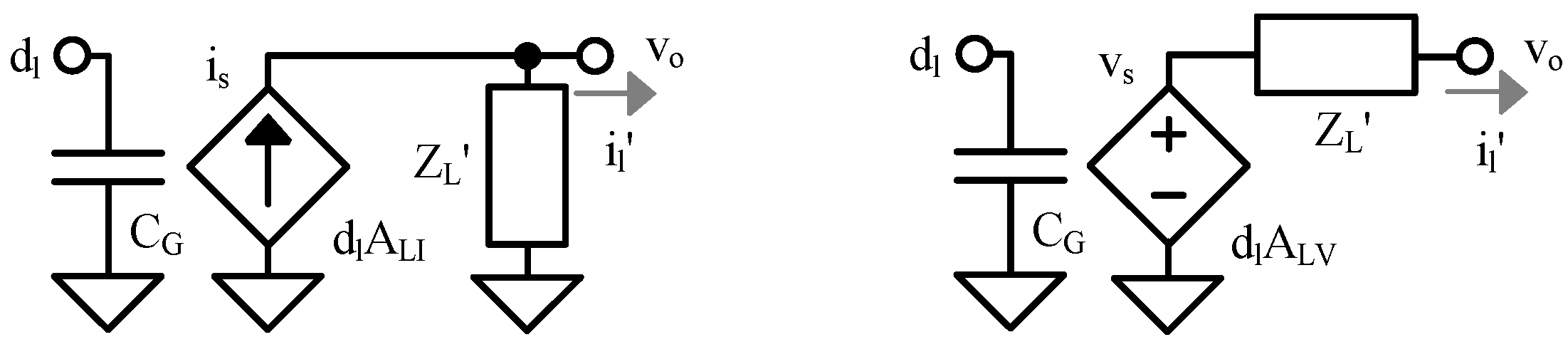
Test Condition: changes in d_L ultimately affect the duty-cycled current i_L′ output by the network. Z_L′ in Figure 9 (left) represents the equivalent impedance that d_O duty-cycles when there are no variations d_l. A_LI in Figure 7 describes the small-signal relationship that maps small changes d_l in d_L to the corresponding variations i_l′ in i_L′ assuming no v_O variations v_o (equivalently, v_O is grounded, as shown in the right-hand side of Figure 9). A_LV is the unloaded voltage that A_LI produces across Z_L′, which is A_LIZ_L′.

Figure 9. Test conditions for deriving Z_L′ and A_LI.

3. Continuous-Conduction Mode

This section presents the model in continuous conduction mode (CCM). Under the assumptions of constant switching-frequency PWM and small perturbations around a steady-state operating point, duty-cycle variations modulate the durations of the energizing and discharging intervals. The modeling procedure then consists of: (i) deriving the expression of the equivalent duty-cycled inductor impedance, including its parasitic resistance; (ii) determining the Norton and Thevenin (current and voltage) gains driving the inductor; and (iii) deriving the small-signal transfer functions of the switched inductor when loaded by a resistance and an output capacitor, including its parasitic resistance.

3.1. Equivalent Impedance

In CCM, Z_L′ in Figure 7 has an inductive component L_X′, and a resistive component R_L′. Because L_X only connects to v_O a D_O fraction of T_SW, the equivalent inductive part of the output impedance of the switched inductor is the duty-cycled inductance L_X′, which loads v_o during T_SW and stores the energy drawn by L_X during T_O. Viewed this way, i_LX is the current drawn by L_X from v_o over the interval T_O (T_O is D_OT_SW), and E_L is the energy stored in L_X after the current ramps up to i_LX:

$$E_L={\displaystyle \frac{L_X{i_{LX}}^2}{2}}=\left({\displaystyle \frac{1}{2}}\right)L_X{\left[\left({\displaystyle \frac{v_o}{L_X}}\right)T_O\right]}^2=\left({\displaystyle \frac{{v_o}^2}{2}}\right)\left({\displaystyle \frac{{D_O}^2}{L_X}}\right){T_{SW}}^2.$$

(4)

In contrast, i_LX′ is the current that L_X′ draws from v_o throughout the entire switching period T_SW, and E_L′ is the energy stored in L_X′ once the inductor current reaches i_LX′:

$${E_L}^{\prime }=\left({\displaystyle \frac{{L_X}^{\prime }}{2}}\right){\left[\left({\displaystyle \frac{v_o}{{L_X}^{\prime }}}\right)T_O\right]}^2=\left({\displaystyle \frac{{v_o}^2}{2}}\right)\left({\displaystyle \frac{1}{{L_X}^{\prime }}}\right){T_{SW}}^2.$$

(5)

But since E_L′ equals the energy provided by E_L, L_X′ can be viewed as a reverse quadratic D_O translation of L_X [17]:

$${L_X}^{\prime }={\displaystyle \frac{L_X}{{D_O}^2}}.$$

(6)

A similar reasoning applies to R_L (series resistance of L_X). R_L dissipates power P_R with v_l, which is equal to the power P_R′ dissipated by the equivalent duty-cycled resistance R_L′ with v_o:

$$P_R={\displaystyle \frac{{v_l}^2}{R_L}}={\displaystyle \frac{{\left(D_O{v}_o\right)}^2}{R_L}}\equiv {P_R}^{\prime }={\displaystyle \frac{{v_o}^2}{{R_L}^{\prime }}}.$$

(7)

Hence, R_L′ is R_L/D_O² [18].

3.2. Unloaded Gain Translations

Inductor Current: in CCM, when d_E increases, t_E lengthens by the same amount t_D shortens, thus increasing i_L. This is the Ohmic translation that A_LI and A_LV model. Under the Norton test conditions that Figure 8 illustrates (Z_L′ is disabled, so there are no v_o variations, and v_IN being an independent voltage source, there are no v_in variations; thus, no v_e or v_d variations), i_L becomes an Ohmic translation of v_L:

$$i_L={\displaystyle \frac{v_L}{Z_L}}={\displaystyle \frac{v_E{d}_E-v_D{d}_D}{Z_L}}={\displaystyle \frac{v_E{d}_E-v_D\left(1-d_D\right)}{Z_L}}={\displaystyle \frac{\left(V_E+V_D\right)d_E-V_D}{Z_L}}.$$

(8)

The small-signal inductor current increase i_l is then the derivative of i_L with respect to d_E:

$$A_L\equiv {\left.{\displaystyle \frac{i_l}{d_l}}\right|}_{v_o=0}={\left.{\displaystyle \frac{{\partial i}_L}{{\partial d}_L}}\right|}_{v_o=0}^{CCM}={\left.{\displaystyle \frac{1}{Z_L}}\left({\displaystyle \frac{{\partial v}_L}{{\partial d}_E}}\right)\right|}_{v_o=0}^{CCM}={\displaystyle \frac{V_E+V_D}{Z_L}}={\displaystyle \frac{q_l/d_l}{T_{SW}}}$$

(9)

i_l corresponds to the extra inductor charge q_l delivered to v_o (as Figure 4 shows). A_L is the component of A_LI in Figure 7 that maps d_l to i_l when small v_O variations v_o are absent.

Duty-Cycled Current: A_LI translates d_l to i_l′ when disabling Z_L′ with zero v_o as Figure 8 shows. Intuitively, A_LI represents the change in inductor current in response to a small perturbation d_l, excluding the loading effect by superposition. This short-circuit i_l′ is a small-signal current source i_s. In boost-derived variants, since i_L and d_O in i_L′ both vary with d_E, i_s carries 2 components, i_o and i_d:

$$\begin{array}{cc}\hfill {\mathrm{A}}_{\mathrm{LI}}& \equiv {\left.{\displaystyle \frac{{\mathrm{i}}_{\mathrm{s}}}{{\mathrm{d}}_{\mathrm{l}}}}\right|}_{{\mathrm{v}}_{\mathrm{o}}=0}={\left.{\displaystyle \frac{{{\partial \mathrm{i}}_{\mathrm{L}}}^{\prime }}{{\partial \mathrm{d}}_{\mathrm{L}}}}\right|}_{{\mathrm{v}}_{\mathrm{o}}=0}={\left.{\displaystyle \frac{\partial \left({\mathrm{i}}_{\mathrm{L}}{\mathrm{d}}_{\mathrm{O}}\right)}{{\partial \mathrm{d}}_{\mathrm{L}}}}\right|}_{{\mathrm{v}}_{\mathrm{o}}=0}\hfill \\ & =\left({\displaystyle \frac{{\partial \mathrm{i}}_{\mathrm{L}}}{{\partial \mathrm{d}}_{\mathrm{L}}}}\right){\mathrm{D}}_{\mathrm{O}}+\left({\displaystyle \frac{{\partial \mathrm{d}}_{\mathrm{O}}}{{\partial \mathrm{d}}_{\mathrm{L}}}}\right){\mathrm{I}}_{\mathrm{L}\left(\mathrm{H}\mathrm{I}\mathrm{\right)}}\hfill \\ & ={{\mathrm{A}}_{\mathrm{L}}\mathrm{D}}_{\mathrm{O}}-{\mathrm{I}}_{\mathrm{L}\left(\mathrm{H}\mathrm{I}\right)}={\displaystyle \frac{{\mathrm{i}}_{\mathrm{l}}-{\mathrm{i}}_{\mathrm{e}}}{{\mathrm{d}}_{\mathrm{l}}}}-{\displaystyle \frac{{\mathrm{i}}_{\mathrm{d}}}{{\mathrm{d}}_{\mathrm{l}}}}={\displaystyle \frac{{\mathrm{i}}_{\mathrm{o}}}{{\mathrm{d}}_{\mathrm{l}}}}-{\displaystyle \frac{{\mathrm{i}}_{\mathrm{d}}}{{\mathrm{d}}_{\mathrm{l}}}}.\hfill \end{array}$$

(10)

The first component is a D_O fraction of i_l, corresponding to the current i_o that the charge q_o in Figure 5 delivers. The second term is zero in buck converters because d_O is 1. In boost converters, however, it becomes an inverting fraction of i_L at its peak value I_L(HI), since d_O equals d_D, which is 1 − d_E. When Δi_L is much lower than i_L, I_L(HI) approximates to I_L = I_L′/D_O.

Model Translations: A_LV in Figure 7 is the unloaded Ohmic translation that A_LI feeds Z_L′ (A_LV is the gain of the voltage source driving the inductor):

$$\begin{array}{cc}\hfill A_{\mathit{LV}}& \equiv {\left.{\displaystyle \frac{v_s}{d_l}}\right|}_{{i_l}^{\prime }=0}={\left.{\displaystyle \frac{\partial v_O}{{\partial d}_L}}\right|}_{{i_l}^{\prime }=0}={A_{\mathit{LI}}}^{\prime }{Z_L}^{\prime }= {\displaystyle \frac{V_E+V_D}{D_O}}-I_{L\left(HI\right)}{Z_L}^{\prime }={\displaystyle \frac{V_E+V_D}{D_O}}-I_{L\left(HI\right)}\left({R_L}^{\prime }+s{L_X}^{\prime }\right)\hfill \\ & =\left({\displaystyle \frac{V_E+V_D}{D_O}}-I_{L\left(HI\right)}{R_L}^{\prime }\right)\left[1-s\left({\displaystyle \frac{I_{L\left(HI\right)}{L_X}^{\prime }}{\frac{V_E+V_D}{D_O}-I_{L\left(HI\right)}{R_L}^{\prime }}}\right)\right]=A_{LV0}\left[1-s\left({\displaystyle \frac{I_{L\left(HI\right)}{L_X}^{\prime }}{A_{LV0}}}\right)\right]\hfill \\ & =A_{LV0}\left(1-{\displaystyle \frac{s}{2\pi z_{DO}}}\right)\hfill \end{array}$$

(11)

Because R_L′ is usually very low, A_LV0 approximates to (V_E + V_D)/D_O. I_L(HI)Z_L′ overcomes and inverts A_LV past the inverting zero z_DO [18]:

$$z_{DO}={\displaystyle \frac{A_{LV0}/I_{L\left(HI\right)}}{{2\pi L_X}^{\prime }}}.$$

(12)

The final component i_d in (10) represents the charge q_e and q_d lost by t_eI_L(HI) across T_SW. Fortunately, i_o is much higher than i_d at low frequency because Z_L in i_o is very low. However, i_l decreases with frequency as Z_L increases with frequency. Because i_d remains constant, it eventually exceeds i_l, causing i_o to drop below i_d past z_DO.

3.3. Direct Small-Signal Model

Figure 10 below illustrates the Thevenin-equivalent model developed in the previous subsection, while Table 2 summarizes the expressions for its components. In CCM, the duty-cycle command d_L controls the switched inductor. This inductor behaves as an equivalent impedance driven by the voltage source v_s, with a gain A_LV relative to d_L.

Figure 10. Switched inductor small-signal direct model in CCM.

Table 2. Component expressions of the CCM small-signal direct model.

Component	Expression
LX′	${\displaystyle \frac{L_X}{{D_O}^2}}$
RL′	${\displaystyle \frac{R_L}{{D_O}^2}}$
ALV	$\left({\displaystyle \frac{V_E+V_D}{D_O}}-I_{L\left(HI\right)}{R}_L\prime \right)\left[1-s\left({\displaystyle \frac{I_{L\left(HI\right)}{L}_X\prime }{\frac{V_E+V_D}{D_O}-I_{L\left(HI\right)}{R}_L\prime }}\right)\right]$

3.4. Loaded Gains

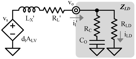
A switched inductor usually connects to a load Z_LD, which typically includes a capacitor C_O with an associated series resistance R_C, and a load resistance R_LD, as Figure 11 depicts. Z_LD exhibits a pole z_LD′ when C_O shorts R_LD and R_C and a zero z_CX when C_O shorts R_C [16]:

$$Z_{LD}={\displaystyle \frac{R_{LD}\left(1+s{R}_C{C}_O\right)}{\left[1+s\left(R_C+R_{LD}\right)C_O\right]}}={\displaystyle \frac{R_{LD}\left(1+\frac{s}{2\pi z_{CX}}\right)}{\left(1+\frac{s}{2\pi {z_{LD}}^{\prime }}\right)}}.$$

(13)

Figure 11. Loaded switched inductor in CCM.

The current that the switched inductor delivers to R_LD is i_LD. The output voltage of the power stage matches the load voltage.

Duty-Cycled Current: when the switched inductor is connected to Z_LD, as Figure 11 shows, it functions as a power stage. The transfer function of L_X, C_O, R_LD, and their parasitics exhibits an LC double pole p_LC with quality factor Q_LC, and a load zero z_LD′ arising when C_O shorts R_LD and R_C. A_G is the transconductance gain from v_s to i_l′. The output current i_l′ to duty cycle d_l gain, defined as A_IL′, is simply:

$$\begin{array}{cc}\hfill A_{IL}^{\prime }& \equiv {\displaystyle \frac{{i_l}^{\prime }}{d_l}}=A_{LV}{A}_G\hfill \\ & =A_{LV}\left({\displaystyle \frac{1}{R_{LD}+{R_L}^{\prime }}}\right)\left[{\displaystyle \frac{\left(1+\frac{s}{2\pi {z_{LD}}^{\prime }}\right)}{1+\frac{1}{Q_{LC}}\left(\frac{s}{2\pi p_{LC}}\right)+{\left(\frac{s}{2\pi p_{LC}}\right)}^2}}\right].\hfill \end{array}$$

(14)

Inductor Current: Deriving the d_l-to-i_l gain requires reconstructing the current waveform to isolate A_L in (10) and accounting for the DC inductor current I_L(HI) flowing into the load impedance Z_LD in Figure 11 [19]:

$$A_{IL}\equiv {\displaystyle \frac{i_l}{d_l}}=\left(A_{LV0}+I_{L\left(HI\right)}{Z}_{LD}\right)\left({\displaystyle \frac{A_G}{D_O}}\right).$$

(15)

i_l′ denotes the current delivered by the power stage, whereas i_l is the inductor current. Although sometimes useful for intermediate analysis, i_l remains an internal signal of the power stage.

Unlike A_IL′, the A_IL gain to i_l excludes z_DO because i_l is not affected by the effect of d_O. Because of the gain reconstruction, the zero z_LD in A_IL shifts to:

$$z_{LD}=\left(A_{LV0}+I_{L\left(HI\right)}{R}_{LD}\right)\left({\displaystyle \frac{{z_{LD}}^{\prime }}{A_{LV0}}}‖{\displaystyle \frac{z_{CX}}{I_{L\left(HI\right)}{R}_{LD}}}\right).$$

(16)

Because R_C is often very low, z_CX is often much higher than z_LD′, so z_LD approximates to z_LD′(1 + I_L(HI)R_LD/A_LV0).

Outputs: The d_l-to-v_o gain A_VO is the gain that i_l′ sets into Z_LD: A_LVA_GZ_LD [16]. The d_l to load current i_LD (in Figure 10) gain A_ILD is then simply A_VO/R_LD.

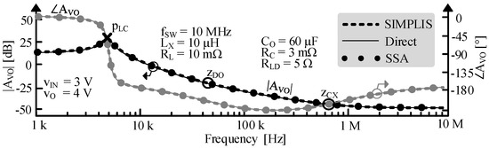
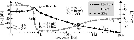
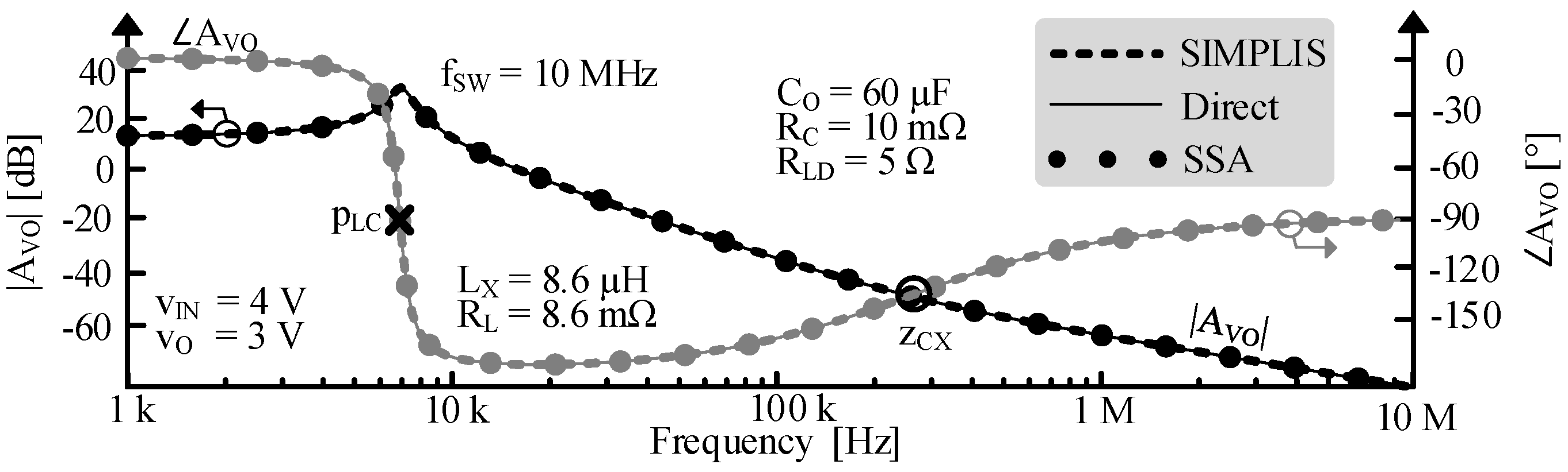
Figure 12 shows the output-voltage-to-duty-cycle gain A_VO for a boost converter. The Bode plots are obtained using the proposed direct model and the state-space averaging (SSA) model [4], with SIMPLIS providing the reference simulated response. Since both Circuit Averaging and Signal Flow Graph approaches are fundamentally derived from the SSA formulation, their transfer functions coincide with those obtained from SSA; therefore, only the SSA, proposed model, and SIMPLIS-based results are plotted for clarity. The resulting curves largely overlap, indicating very close agreement between the analytical models and the simulation. The direct model is shown using a thin solid trace, the SIMPLIS simulation using a medium dashed trace, and the SSA model using a thick dotted trace, with magnitude plotted in black and phase in dark gray. Figure 13 presents the corresponding results for a buck converter under the same operating conditions: z_DO is absent, and p_LC shifts to the left, because d_O is 1. As in the boost case, SIMPLIS and the SSA [4] and direct models exhibit essentially identical accuracy. Table 2 below summarizes key parameters of the Bode plots. Despite the inherent uncertainties associated with reading values from simulated Bode plots, theoretical values closely match the simulated ones.

Figure 12. Simulated and calculated CCM gain to v_o for boost.

Figure 13. Simulated and calculated CCM gain to v_o for buck.

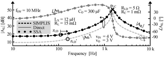
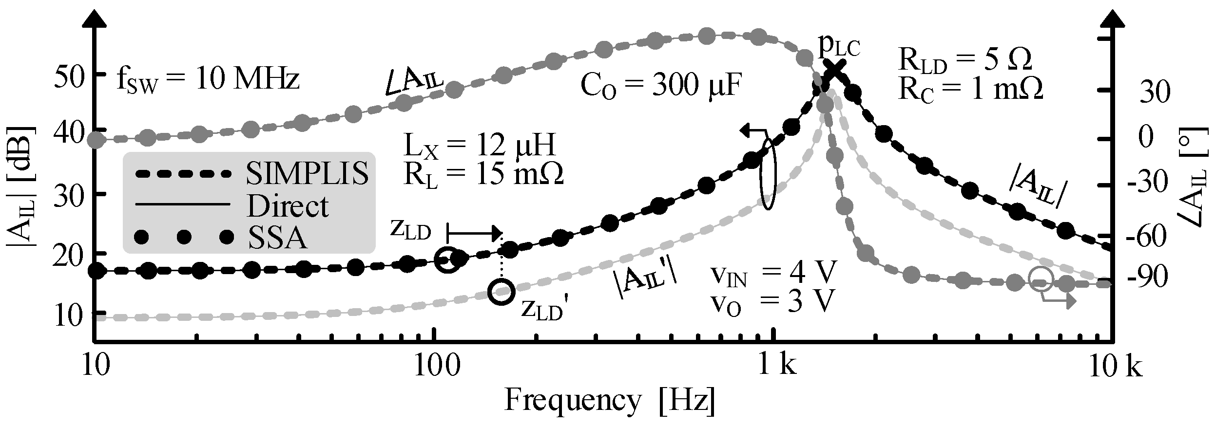
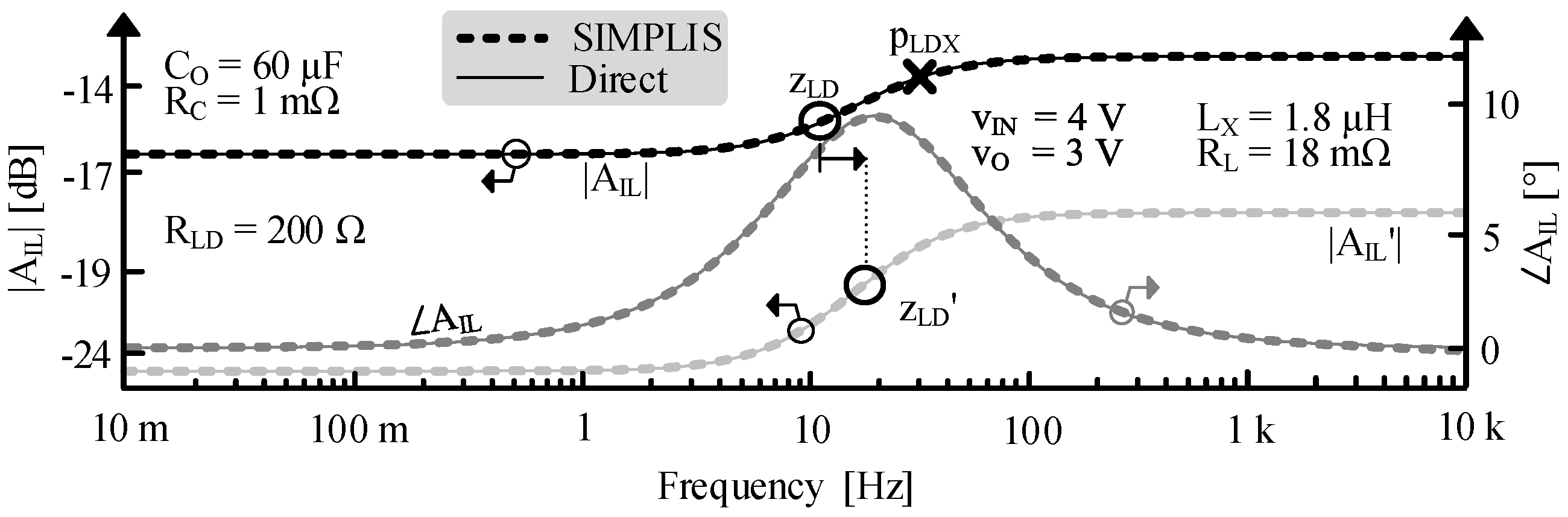
Figure 14 shows the inductor-current-to-duty-cycle gain A_IL for a buck–boost converter. The Bode plots include SIMPLIS, the proposed direct model, and the state-space averaging (SSA) model [18], with parameters summarized in Table 3. The resulting curves largely overlap, indicating very close agreement between the two modeling approaches and SIMPLIS. The magnitude /A_IL′/ is also shown in light gray to highlight the shift of z_LD in A_IL, as described by (15).

Figure 14. Simulated and calculated CCM gain to i_l for buck–boost.

Table 3. Summary of CCM gains Bode plots values.

Parameters	SSA	Direct	SIMPLIS
CCM Boost: vo/dl
AVO0	14.9 dB	14.9 dB	14.9 dB
pLC	4.9 kHz	4.9 kHz	5 kHz
zDO	44.6 kHz	44.7 kHz	45 kHz
zCX	885 kHz	885 kHz	880 kHz
CCM Buck: vo/dl
AVO0	12.0 dB	12.0 dB	12.0 dB
pLC	7.0 kHz	7.0 kHz	7.0 kHz
zCX	265 kHz	265 kHz	260 kHz
CCM Buck–Boost: il/dl
AIL0	15.7 dB	15.7 dB	15.7 dB
pLC	1.5 kHz	1.5 kHz	1.5 kHz
zLD	150 Hz	150 Hz	150 Hz
DCM Boost: vo/dl
AVO0	19.1 dB	19.1 dB	19.1 dB
pLDX	40.0 Hz	40.0 Hz	40 Hz
zCX	15.9 kHz	15.9 kHz	16 kHz
DCM Buck–Boost: il/dl
AIL0	N/A	−16 dB	−16 dB
zLD	N/A	27.0 Hz	27 Hz
pLDX	N/A	19.0 Hz	20 Hz

4. Discontinuous-Conduction Model

In DCM, in order to save power, the controller typically turns all power switches off after the inductor has completely discharged, thereby introducing a zero-current interval following the conduction period. The fact that the inductor fully drains before the start of the next cycle means that i_s loses q_e with d_O, but no part of q_d that would otherwise invert and alter i_s in CCM. As a result, A_LI and A_LV in DCM do not include z_DO. It also means that a longer t_E will require a proportionately longer t_D to drain the inductor, because the v_E and v_D that project i_L are static. Therefore, the portion of v_E applied to L_X by d_E cancels out the portion of v_D applied by d_D. As a result, the net small-signal voltage v_l across L_X is zero:

$$v_l=v_E\left({\displaystyle \frac{t_e}{T_{SW}}}\right)-v_D\left({\displaystyle \frac{t_d}{T_{SW}}}\right)=0.$$

(17)

Since the projections of v_E and v_D onto the inductor current remain constant, the ratios of t_e/t_d and T_E/T_D are identical. Changes in t_E cause corresponding changes in t_C (and t_D), which track proportionally with both T_E and T_C. As a result, the ratio t_e/T_E, denoted as k_s, matches the ratio t_c/T_C:

$$k_s\equiv {\displaystyle \frac{t_e}{T_E}}={\displaystyle \frac{t_d}{T_D}}={\displaystyle \frac{t_c}{T_C}}={\displaystyle \frac{i_{l\left(pk\right)}}{I_{L\left(PK\right)}}}.$$

(18)

Therefore, d_E is equal to its static value D_E, and exhibits no small-signal variations d_e:

$$d_E={\displaystyle \frac{T_E+t_e}{T_C+t_c}}={\displaystyle \frac{T_E+t_e}{T_E+t_e+T_D+t_d}}={\displaystyle \frac{T_E\left(1+k_s\right)}{T_E\left(1+k_s\right)+T_D\left(1+k_s\right)}}={\displaystyle \frac{T_E}{T_C}}=D_E.$$

(19)

By extension from (2), k_s also aligns with the fraction of the peak inductor current i_l(pk) relative to its steady-state peak I_L(PK). In DCM, the small-signal duty-cycle command d_l (which is no longer equal to d_e) effectively modulates the amount of charge drawn by the inductor. The proposed DCM model assumes constant-frequency operation (i.e., fixed switching period) rather than frequency modulation. Regulation is achieved by modulating the inductor charge per cycle through duty-cycle variation, both under small-signal perturbations and under large-signal load changes. In this framework, the switching frequency remains constant while the amount of energy transferred per cycle is adjusted to meet the load demand.

4.1. Equivalent Impedance

Similarly to CCM, Z_L′ is the equivalent output impedance of the switched inductor when there are no small-signal variations in d_L. Namely, it is the impedance seen into L_X when both t_C and t_SW are static, and L_X connects to v_O for a d_O fraction of t_C. Because v_L across L_X is zero, Z_L′ is insensitive to frequency. As a result, Z_L′ behaves like a duty-cycled resistance R_L′, which loads v_O over T_SW by the amount of energy that L_X draws during the d_O portion of T_C. In DCM, the output effectively sees the inductance as an equivalent loading resistance R_L′.

Viewed this way, i_LX is the current that L_X draws from v_O during the d_O portion of T_C, and E_L is the energy stored in L_X once the inductor current i_L ramps up to i_LX:

$$E_L=\left({\displaystyle \frac{1}{2}}\right)L_X{i_{LX}}^2=\left({\displaystyle \frac{L_X}{2}}\right){\left[\left({\displaystyle \frac{v_o}{L_X}}\right){D_{O}T}_C\right]}^2=\left({\displaystyle \frac{{v_o}^2}{2}}\right)\left({\displaystyle \frac{{D_O}^2}{L_X}}\right){T_C}^2.$$

(20)

This E_L is the power P_R′ that R_L′ burns across T_SW [20]:

$${P_R}^{\prime }=\left({\displaystyle \frac{{v_o}^2}{{R_L}^{\prime }}}\right)\equiv {\displaystyle \frac{E_L}{T_{SW}}}=\left({\displaystyle \frac{{v_o}^2}{2}}\right)\left({\displaystyle \frac{{D_O}^2}{L_X}}\right)\left({\displaystyle \frac{{T_C}^2}{T_{SW}}}\right)={\displaystyle \frac{{v_o}^2{i}_O{D}_O}{v_E‖v_D}}.$$

(21)

Thus, R_L′ is the frequency-independent equivalent of L_X′ in CCM. The duty-cycled contribution of the series resistance R_L increases R_L′, but typically only slightly:

$${R_L}^{\prime }={\displaystyle \frac{v_E‖v_D}{i_O{D}_O}}+{\displaystyle \frac{R_L}{{D_O}^2}}.$$

(22)

4.2. Unloaded Gain Translations

Because the inductor current returns to zero at the end of each switching period in DCM, the energy transferred to the output during each cycle is determined by the peak inductor current reached during the energizing interval. Under the assumption that the inductor remains in DCM, it behaves like a current source delivering charge to the output (with a gain with respect to d_l given by A_LI). The equivalent resistance R_L′ then represents the effective loading seen by the output, corresponding to the Norton equivalent resistance of the source.

Duty-Cycled Current: A_LI translates the small-signal variation d_l into i_l′ when Z_L′ is disabled; in other words, when v_O is 0, as Figure 9 shows. While i_l′ outputs all the charge q_L that L_X delivers, it excludes the static component Q_L. Since i_L ramps linearly, both q_L and Q_L correspond to the areas under the triangular waveforms traced by i_L and I_L in Figure 6.

q_L′s t_C and i_L(PK) are T_C and I_L(PK) plus corresponding k_s fractions of T_C and I_L(PK) because t_c and i_l(pk) scale with T_C and I_L(PK):

$$\begin{array}{cc}\hfill q_l& =q_L-Q_L=0.5t_C{i}_{L\left(PK\right)}-0.5T_C{I}_{L\left(PK\right)}\hfill \\ & =0.5T_C\left(1+k_s\right)I_{L\left(PK\right)}\left(1+k_s\right)-0.5T_C{I}_{L\left(PK\right)}\hfill \\ & =0.5T_C{I}_{L\left(PK\right)}{\left({k_s}^2+2k_s\right)}^2\approx T_C{I}_{L\left(PK\right)}{k}_s=t_c{I}_{L\left(PK\right)}.\hfill \end{array}$$

(23)

v_o then receives the small-signal charges q_o, a duty-cycle portion of q_l:

$$q_o=q_D-Q_D\approx T_D{I}_{L\left(PK\right)}{k}_d=t_d{I}_{L\left(PK\right)}.$$

(24)

Since k_s is a small fraction and t_e/t_c = D_E, the term 2k_s dominates over k_s², and t_c can be approximated as t_e/D_E. As a result, q_L is approximately the rectangular area defined by t_c and I_L(PK) in Figure 6, so A_LI is i_s/d_l, which is roughly q_D/(T_SWd_l):

$$\begin{array}{cc}\hfill A_{LI}& \equiv {\left.{\displaystyle \frac{{i_l}^{\prime }}{d_l}}\right|}_{v_o=0}={\displaystyle \frac{i_s}{d_l}}={\displaystyle \frac{q_{\frac{l}{d}}}{d_l{T}_{SW}}}\approx {\displaystyle \frac{t_c{D}_O{I}_{L\left(PK\right)}}{d_l{T}_{SW}}}={\displaystyle \frac{t_e{D}_O{I}_{L\left(PK\right)}}{d_l{D}_E{T}_{SW}}}\hfill \\ & =\left({\displaystyle \frac{I_{L\left(PK\right)}}{D_E}}\right)D_O.\hfill \end{array}$$

(25)

4.3. Direct Small-Signal Models

Figure 15 below shows the models that the previous subsection develops, while Table 4 summarizes the expressions for its components. In DCM, a Norton equivalent model models the power stage as a current-sourced resistor. This model can be transformed into a Thevenin equivalent model.

Figure 15. Switched inductor small-signal direct models in DCM.

Table 4. Component expressions of the DCM small-signal direct model.

Component	Expression
RL′	${\displaystyle \frac{v_E‖v_D}{i_O{D}_O}}+{\displaystyle \frac{R_L}{{D_O}^2}}$
ALI	$\left({\displaystyle \frac{I_{L\left(PK\right)}}{D_E}}\right)D_O$

4.4. Loaded Gains

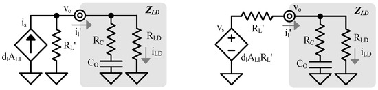
As in Section 3.4, the switched inductor load constitutes a power stage operating in DCM. Figure 16 illustrates the corresponding loaded models. The Norton direct model is shown on the left, and the Thevenin direct model on the right.

Figure 16. Loaded switched inductor in DCM: Norton (left) and Thevenin (right).

Duty-Cycled Current: similarly to CCM, A_G is the transconductance gain from v_s to i_l′ and depends on the nature of the load. When the power stage feeds Z_LD like in Figure 16, A_G is [21]:

$$\begin{array}{cc}\hfill A_G& \equiv {\displaystyle \frac{{i_l}^{\prime }}{v_s}}\approx {\displaystyle \frac{1}{{R_L}^{\prime }+R_{LD}}}\left\{{\displaystyle \frac{1+s\left(R_C+{R_L}^{\prime }\right)C_O}{1+s\left[R_C+\left(R_{LD}‖{R_L}^{\prime }\right)\right]C_O}}\right\}\hfill \\ & =A_{G0}\left({\displaystyle \frac{1+\frac{s}{2\pi {z_{LD}}^{\prime }}}{1+\frac{s}{2\pi p_{LDX}}}}\right).\hfill \end{array}$$

(26)

A_IL′, the output current i_l′ to duty cycle d_l gain, is read from Figure 15:

$${A_{IL}}^{\prime }\equiv {\displaystyle \frac{{i_l}^{\prime }}{d_l}}=A_{LI}{{R_L}^{\prime }A}_G.$$

(27)

Inductor Current: unlike in CCM, only q_e stops reaching the output when d_e increases. This is why A_IL does not show a 1/D_O factor in the reconstructed current waveform:

$$A_{IL}\equiv {\displaystyle \frac{i_l}{d_l}}=A_{LI}{{R_L}^{\prime }A}_G+I_{L\left(PK\right)}.$$

(28)

Thus, the zero z_LD in A_IL in DCM shifts to:

$$z_{LD}=\left(A_{LI}{{R_L}^{\prime }A}_{G0}+I_{L\left(PK\right)}\right)\left({\displaystyle \frac{{z_{LD}}^{\prime }}{A_{LI}{{R_L}^{\prime }A}_{G0}}}‖{\displaystyle \frac{p_{LDX}}{I_{L\left(PK\right)}}}\right).$$

(29)

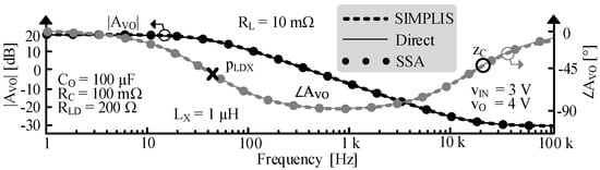
Outputs: by defining A_Z as the parallel combination of R_L′ and Z_LD, A_VO in DCM becomes A_LIA_Z, and A_ILD is A_VO/R_LD. Figure 17 below shows A_VO for a boost in DCM [22]. The responses obtained from SIMPLIS, the SSA, and the proposed direct model largely overlap, indicating very close agreement between the two approaches.

Figure 17. Simulated and calculated DCM gain to v_o for boost.

Figure 18 shows A_IL for a buck–boost converter under the same load conditions, with key parameters listed in Table 3. The response predicted by the proposed direct model closely overlaps the SIMPLIS simulation, demonstrating excellent agreement. Figure 18 also plots the magnitude |A_IL′| in light gray to highlight the shift of z_LD in A_IL in DCM, as described by (29). To the authors′ knowledge, no SSA model for A_IL in this operating mode has been reported in the literature.

Figure 18. Simulated and calculated DCM gain to i_l for buck–boost.

5. Conclusions

This work presents a direct small-signal AC response model for switched inductors in both DCM and CCM that preserves circuit-level insight while maintaining the accuracy of established modeling approaches. The voltage and current gains derived from the proposed model closely match those obtained using state-space averaging, as confirmed by Bode-plot comparisons that show nearly overlapping frequency responses. In both conduction modes, the method enables the systematic derivation of the duty-cycle-to-output-voltage, duty-cycle-to-output-current, and duty-cycle-to-inductor-current transfer functions within a unified circuit framework. The model accurately captures the LC double pole and associated zeros, including the shift of the load-related zero in the reconstructed duty-cycle-to-inductor-current gain. In addition to supporting the derivation of these key gains, the proposed approach retains direct circuit interpretability and remains straightforward to use, analyze, and simulate. These characteristics suggest that the method could facilitate control-loop design and may be suitable for integration into automated synthesis or optimization frameworks. Furthermore, the analytical expression obtained for the DCM duty-cycle-to-inductor-current gain contributes to clarifying this relationship within the existing literature.

References

- Chen, W.-C.; Chen, C.-C.; Yao, C.-Y.; Yang, R.-J. A Fast-Transient Wide-Voltage-Range Digital-Controlled Buck Converter with Cycle-Controlled DPWM. IEEE Trans. Very Large Scale Integr. Syst. 2016, 24, 17–25. [Google Scholar] [CrossRef] [Scilit]
- Rincón-Mora, G.A. Analog IC Design with Low-Dropout Regulators; McGraw-Hill: New York, NY, USA, 2009. [Google Scholar]
- Maksimovic, D.; Cuk, S. A Unified Analysis of PWM Converters in Discontinuous Modes. IEEE Trans. Power Electron. 1991, 6, 476–490. [Google Scholar] [CrossRef] [Scilit]
- Sun, J.; Mitchell, D.; Greuel, M.; Krein, P.; Bass, R. Averaged Modeling of PWM Converters Operating in Discontinuous Conduction Mode. IEEE Trans. Power Electron. 2001, 16, 482–492. [Google Scholar] [CrossRef] [Scilit]
- Surya, S.; Srinivasan, M.K.; Williamson, S. Modeling of Average Current in Non-Ideal Buck and Synchronous Buck Converters for Low Power Application. Electronics 2021, 10, 2672. [Google Scholar] [CrossRef] [Scilit]
- Vorpérian, V. Simplified Analysis of PWM Converters Using Model of PWM Switch Part I & II. IEEE Trans. Aerosp. Electron. Syst. 1990, 26, 490–505. [Google Scholar]
- Paduvalli, V.; Taylor, R.J.; Balsara, P.T. Analysis of Zeros in a Boost DC–DC Converter: State Diagram Approach. IEEE Trans. Circuits Syst. II Expr. Briefs 2017, 64, 550–554. [Google Scholar] [CrossRef] [Scilit]
- Saini, D.K.; Kazimierczuk, M.K. Open-loop transfer functions of buck–boost converter by circuit-averaging technique. IET Power Electron. 2019, 12, 2858–2864. [Google Scholar] [CrossRef] [Scilit]
- Ki, W. Signal Flow Graph in Loop Gain Analysis of DC-DC PWM CCM Switching Converters. IEEE Trans. Circuits Sys. I 1998, 45, 644–655. [Google Scholar]
- Ma, Y.; Smedley, K. Switching Flow-Graph Nonlinear Modeling Method for Multistate-Switching Converters. IEEE Trans. Power Electron. 1997, 12, 854–861. [Google Scholar]
- Veerachary, M. Analysis of Fourth-Order DC-DC Converters: A Flow Graph Approach. IEEE Trans. Ind. Electron. 2008, 55, 133–141. [Google Scholar] [CrossRef] [Scilit]
- Corti, F.; Laudani, A.; Lozito, G.M.; Reatti, A.; Bartolini, A.; Ciani, L.; Kazimierczuk, M.K. Modelling of a pulse-skipping modulated DC–DC buck converter. IET Power Electron. 2022, 16, 243–254. [Google Scholar] [CrossRef] [Scilit]
- Kroičs, K.; Gaspersons, K.; Zdanowski, M. Modular DC-DC Converter with Adaptable Fast Controller for Supercapacitor Energy Storage Integration into DC Microgrid. Electronics 2025, 14, 700. [Google Scholar] [CrossRef] [Scilit]
- Abbas, G.; Gu, J.; Farooq, U.; Abid, M.I.; Raza, A.; Asad, M.U.; Balas, V.E.; Balas, M.E. Optimized Digital Controllers for Switching-Mode DC-DC Step-Down Converter. Electronics 2018, 7, 412. [Google Scholar] [CrossRef] [Scilit]
- Firpo, P.; Ravera, A.; Oliveri, A.; Lodi, M.; Storace, M. Use of a Partially Saturating Inductor in a Boost Converter with Model Predictive Control. Electronics 2023, 12, 3013. [Google Scholar] [CrossRef] [Scilit]
- Yao, J.; Abramovitz, A. Fast SFG Modeling of Integrated Converters. IEEE J. Emerg. Sel. Top. Power Electron. 2017, 5, 1008–1019. [Google Scholar] [CrossRef] [Scilit]
- Kim, S.; Rincon-Mora, G.A.; Kwon, D. Extracting the frequency response of switching DC-DC converters in CCM and DCM from time-domain simulations. In Proceedings of the 2011 International SoC Design Conference, Jeju, Republic of Korea, 17–18 November 2011; pp. 385–388. [Google Scholar]
- Cuk, S. Modeling, Analysis, and Design of Switching Converters. Ph.D. Thesis, California Institute of Technology, Pasadena, CA, USA, November 1976. [Google Scholar]
- Zhu, M.; Luo, F.L. Graphical Analytical Method for Power DC-DC Converters: Averaging Binary Tree Structure Representation. IEEE Trans. Power Electron. 2007, 22, 701–705. [Google Scholar] [CrossRef] [Scilit]
- Kwon, D.; Rincon-Mora, G.A. Operation-based signal-flow AC analysis of switching DC-DC converters in CCM and DCM. In Proceedings of the 2009 52nd IEEE International Midwest Symposium on Circuits and Systems, Cancun, Mexico, 2–5 August 2009; pp. 957–960. [Google Scholar]
- Erickson, R.; Maksimović, D. Fundamentals of Power Electronics, 2nd ed.; Springer Science & Business Media, LLC: New York, NY, USA, 2001. [Google Scholar]
- Ćuk, S.; Middlebrook, R. A general unified approach to modeling switching dc-to-dc converters in discontinuous conduction mode. In Proceedings of the IEEE Power Electronics Specialists Conference, Palo Alto, CA, USA, 14–16 June 1977; pp. 36–57. [Google Scholar]
Disclaimer/Publisher’s Note: The statements, opinions and data contained in all publications are solely those of the individual author(s) and contributor(s) and not of MDPI and/or the editor(s). MDPI and/or the editor(s) disclaim responsibility for any injury to people or property resulting from any ideas, methods, instructions or products referred to in the content. |
© 2026 by the authors. Licensee MDPI, Basel, Switzerland. This article is an open access article distributed under the terms and conditions of the Creative Commons Attribution (CC BY) license.