Improved Jiles–Atherton Magnetic Core Model and Its SPICE Implementation

Abstract

This research presents an improved version of the Jiles–Atherton (J.-A.) ferromagnetic core model. The presented model eliminates the distortion of minor hysteresis loops and achieves better matching with measured data for minor loops—a well-known weak point of the unmodified J.-A. model. The proposed J.-A. model extension is backward compatible with the basic model version and requires two or four additional parameters. In addition to providing model equations, this paper considers the practical implementation of the improved J.-A. model using SPICE circuit simulation tools. The developed modular SPICE macromodel set is compatible with both open-source and proprietary circuit simulation software, and it allows for the construction of transformer schematics of any complexity. The proposed model shows a good match with measurement results for hysteresis loops and transient waveforms in transformer circuits.

1. Introduction

Circuit simulation tools based on SPICE [1] are the industrial standard for electronic equipment design. There exist a number of proprietary and open-source [2] implementations of SPICE. Circuit simulators based on SPICE provide a number of basic linear and nonlinear component models such as lumped devices, transistors, and dependent and independent sources. The transformers do not belong to standard set of SPICE devices, and they require the design of a custom model. SPICE simulation tools provide an inductive coupling device. This device could be attached to the inductor model, and it allows for the design of an ideal transformer through known primary and secondary inductance and coupling coefficients. This approach has the disadvantage that magnetic core properties and hysteresis are not taken into account. Accounting for the saturation and hysteresis in the magnetic core is essential for the proper simulation of power electronic devices [3,4,5], including DC/DC convertors [6] and silicon carbide (SiC) circuits [7,8].

There exist a number of magnetic hysteresis model implementations, including the Preisach [9], Chan [10], Jiles–Atherton [11,12,13], and energy-based (EB) [14,15] models. All of these models are widely used for the simulation of hysteresis effects in different technical and scientific applications. The Preisach model shows good results in the simulation of asymmetrical hysteresis loops [16] and is often used for ferroelectrics simulations [17]; it can also be integrated with finite element analysis software [18,19]. The energy-based hysteresis model finds application in the simulation of pulsed power systems, taking into account the eddy currents [20] and vector hysteresis processes [21]. The Chan model can be used for hysteresis and magnetization curve simulation of soft magnetic amorphous alloys [22]. However, these three models are not very popular for the simulation of circuits containing inductors and transformers with ferromagnetic cores. The Jiles–Atherton (J.-A.) model [23,24] is the most frequently used hysteresis model for circuit simulation tasks [3,4,5]. There exist a number of J.-A. model extensions [25] providing better experimental data matching, and there are a number of open and commercial implementations of this model. For example, [26] presents a transformer model in the form of a SPICE sub-netlist based on J.-A. hysteresis equations. Nevertheless, the existing circuit simulation software has some problems related to the implementation of magnetic core models.

• The LTSpice freeware circuit simulator does not provide a core model taking into account magnetic hysteresis in the libraries shipped with its application.
• The MicroCAP simulator (proprietary license) provides a magnetic core model based on the J.-A. model, but the development of this simulator has been discontinued, and this software may cease to be operational on new operating systems. MicroCAP provides only a magnetic core model implemented in binary form, but not in the form of a SPICE netlist. This prevents the use of this model with other SPICE simulators.
• The Ngspice [27] circuit simulator (open-source license) provides an XSPICE implementation core model taking into account magnetic hysteresis based on piecewise linear (PWL) functions. This model is not compatible with the J.-A. model.

All of the models mentioned in the previous paragraph imply the uniform distribution of the magnetic flux in the core cross-sectional area, as well as an absent or narrow air gap compared with the magnetic path length. This is not a limiting factor for practical usage of the mentioned J.-A. model implementations because most of the transformers used in electronic devices satisfy these conditions.

Summarizing the above, we can conclude that the development of unified open implementations of the J.-A. model that are compatible with free circuit simulation tools is a pressing task. The implementations of the J.-A. model used by existing circuit simulation software face a number of problems. The J.-A. model provides good representation of a major hysteresis loop, where the core operates near saturation, but shows a significant mismatch for minor hysteresis loops where saturation is not reached. Proprietary circuit simulators are also affected by this problem.

The aforementioned issues could be resolved using advanced models such as EB [14] or modified Preisach [28], but new models are not compatible with the J.-A. model’s parameter set. Another approach [29] implies the conversion of model parameters, but this procedure may be complex. Switching to a new model would require the extraction of parameters from scratch and make it impossible to reuse the existing libraries. There exist a number of J.-A. model modifications [30,31,32] resolving the issues of matching with minor loops. The common point of all mentioned modifications is adding the model parameters depending on magnetic flux density value to the tips of the hysteresis loop. While the mentioned papers provide equations for the modified J.-A. model, the SPICE implementation details of the proposed modification are not fully described. Furthermore, the modified model proposed by [30] compares the simulated and measured hysteresis loops, but it does not compare the time-domain waveform simulation with the measured waveform. This comparison is important for practical applications.

Summarizing the above, the novelty of the present research is as follows:

• Proposing SPICE macromodels implementing the J.-A. model for magnetic core and modular transformer models. This implementation is compatible with open-source SPICE implementations such as Ngspice.
• Proposing modified equations for J.-A. models to resolve the issues with false saturation at low excitation levels. The equation modifications are supported by equivalent circuit implementation.
• Proposing SPICE implementation of the modified J.-A. model. The simulation results are verified by hysteresis loops and transient waveform measurement data.

The rest of this paper is organized as follows: Section 2 provides the equations and SPICE implementation of an unmodified J.-A. ferromagnetic core model and winding model. Section 3 proposes the modification of the J.-A. model to eliminate the problem with false saturation at minor hysteresis loops and provides its SPICE implementation. Section 4 provides a verification of the proposed improved J.-A. model and compares simulated and measurement data for hysteresis loops and transient waveforms. Finally, Section 5 presents the outcomes of this paper and the summary of the achieved results.

2. Basic Transformer SPICE Macromodel

2.1. Basic Jiles–Atherton Ferromagnetic Core Model Equations

The Jiles–Atherton model was used to describe the anhysteric magnetization of the core and hysteresis. The model equations are given below. The anhysteric magnetization $M_a$ could be computed based on the intermediate parameter $H_e$, depending on magnetic field strength and total magnetization M:

$$H_e=H+\alpha M$$

(1)

where $\alpha$ is a dimensionless parameter. The anhysteric magnetization $M_a$ could be expressed using the Langevin function $M_a=L\left(H\right)$. If the $H_e/A$ ratio is less than $0.1$,

$$M_a=M_s{\displaystyle \frac{H}{3A}}$$

(2)

If the $H_e/A$ ratio is greater than $0.1$,

$$M_a=M_s\left(coth\left({\displaystyle \frac{H}{A}}\right)-{\displaystyle \frac{A}{H}}\right)$$

(3)

where $M_s$ is the magnetization saturation (A/m) and A is the domain wall density (model parameter expressed in A/m).

The equation for the total magnetization follows the approach shown in [8]:

$$M={\displaystyle \frac{1}{1+C}}{M}_{irr}+{\displaystyle \frac{C}{1+C}}{M}_a$$

(4)

where C is the magnetization reversibility (model parameter without dimension unit) and $M_{irr}$ is an irreversible magnetization component that can be computed from the differential equation

$${\displaystyle \frac{d{M}_{irr}}{d{H}_e}}={\displaystyle \frac{M_a-M_{irr}}{\delta K}}$$

(5)

where K is a domain pinning model parameter expressed in A/m, and $\delta$ is a directional parameter and should be set to +1 or −1 depending on the magnetic field strength change direction:

$$\delta =\mathrm{sgn}(dH/dt)$$

(6)

The magnetic flux density can be computed from the magnetic field strength and total magnetization as follows:

$$B={\mu }_0(H_e+M)$$

(7)

where ${\mu }_0$ is the absolute magnetic permittivity of the vacuum.

Summarizing all of the above, the hysteresis can be described by the following ordinary differential equation (ODE) [23,24]:

$${\displaystyle \frac{dM}{dH}}={\displaystyle \frac{1}{1+C}}·{\displaystyle \frac{M_a-M}{\delta K-\alpha (M_a-M)}}+{\displaystyle \frac{C}{1+C}}·{\displaystyle \frac{d{M}_a}{dH}}$$

(8)

This form of the J.-A. model does not take into the account effects as such eddy currents or the frequency and temperature dependency of the magnetic core parameters. The hysteresis loop form simulated using this model does not depend on frequency. This means that this model should be used within the frequency range specified by the magnetic core material vendor to achieve a good match. This is not a limiting factor preventing the usage of such model forms because proprietary circuit simulation software also does not provide frequency-dependent hysteresis loop models.

2.2. Ferromagnetic Core Equivalent Circuit

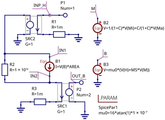
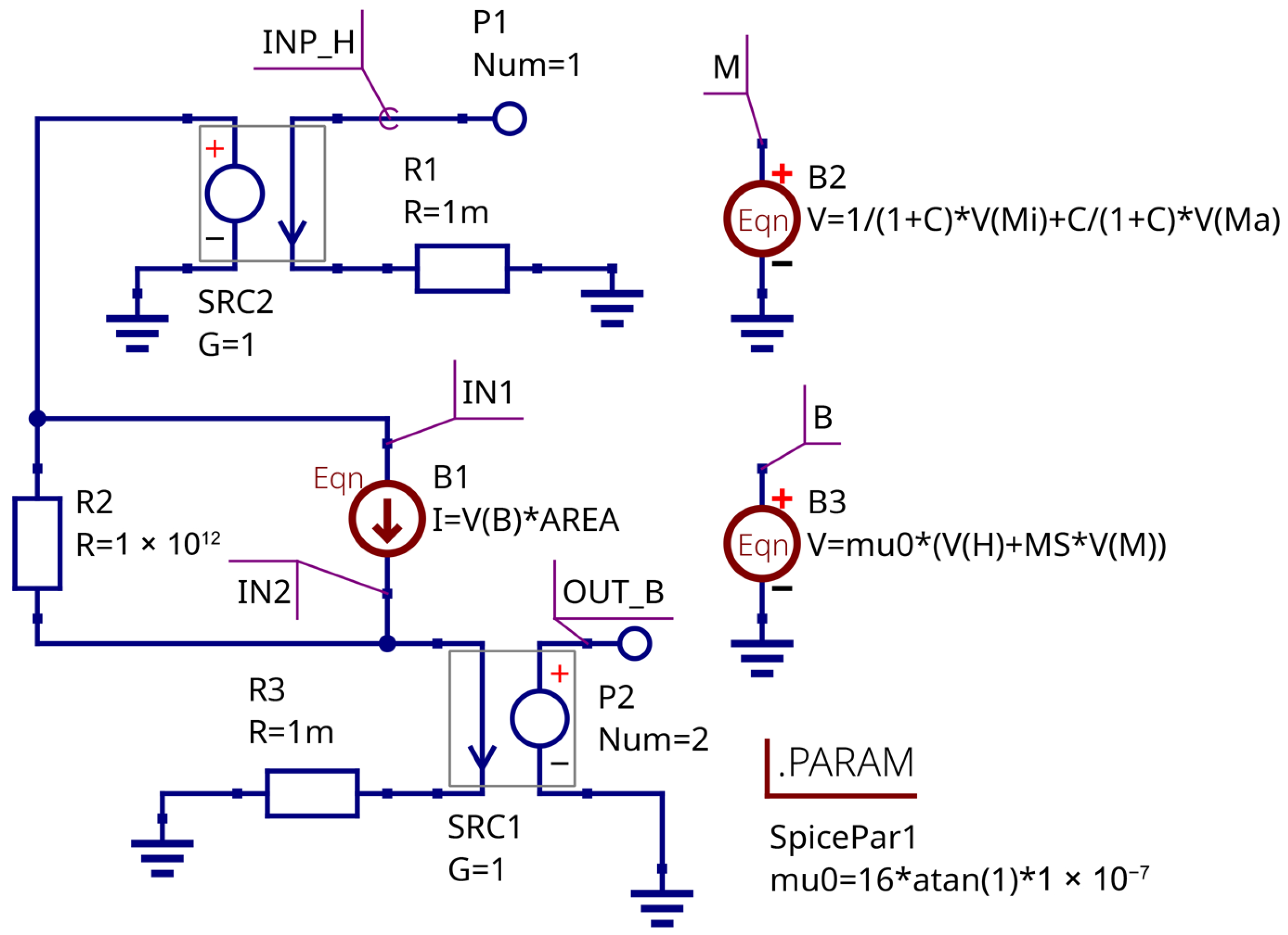
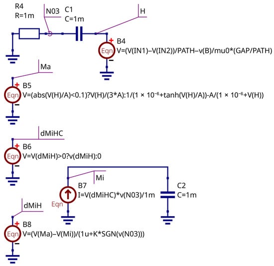
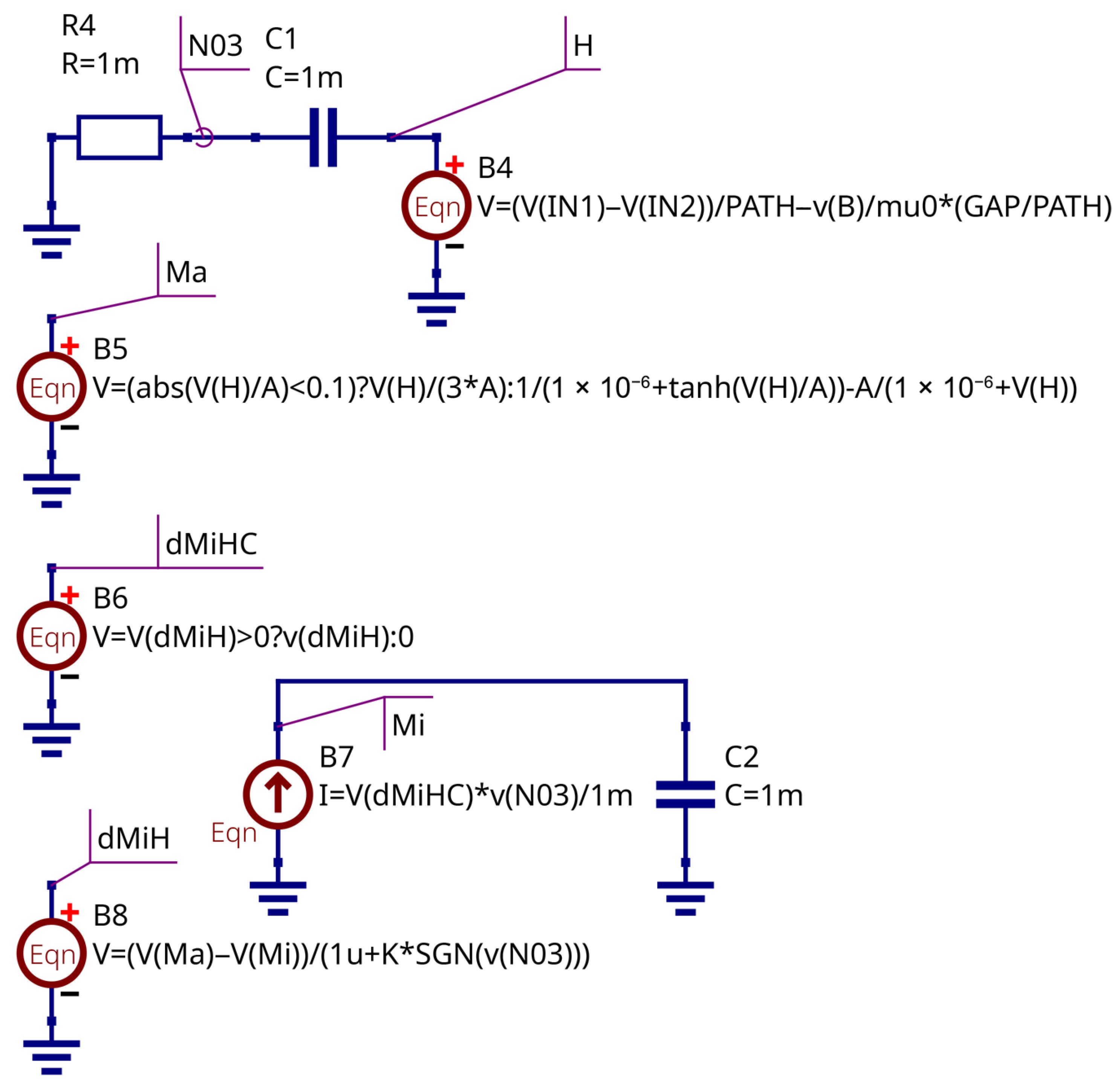
The system of Equations (1)–(7) can be solved numerically using a SPICE-compatible circuit simulator and equivalent circuit representation. The equations may be replaced by a set of equation-defined voltage and current sources. The equivalent circuit implementing the J.-A. magnetic core model is shown in Figure 1 and Figure 2. The Qucs-S open-source circuit simulation tool with the Ngspice backend was used for the model design and debugging.

Figure 1. Magnetic core equivalent circuit: Input and output stage.

Figure 2. Magnetic core equivalent circuit: Differentiation and hysteresis computation stage.

The core model has two terminals: input, representing the magnetic field strength H; and output, representing the magnetic flux $\mathsf{\Phi }$. The controlled sources with unity gain serve to isolate the input and output from external circuits. The controlled source B1 computes the magnetic flux $\mathsf{\Phi }$ as follows:

$$\mathsf{\Phi }=BS$$

(9)

where the S is the core cross-section area.

The total M, irreversible $M_{irr}$, and anhysteric $M_a$ are represented as the virtual voltages and computed by equation-defined voltage sources B2, B5, and B7, respectively. The magnetic flux density B is also the virtual voltage and is computed via Equation (7). Resistors R1, R2, and R3 are the convergence helpers; their values are selected according to the recommendations provided in [26]. The circuit B4C1R4 serves to obtain the time derivative of the magnetic field strength using the fundamental properties of the capacitor current. The source B8 represents Equation (5).

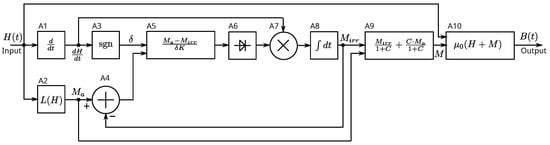
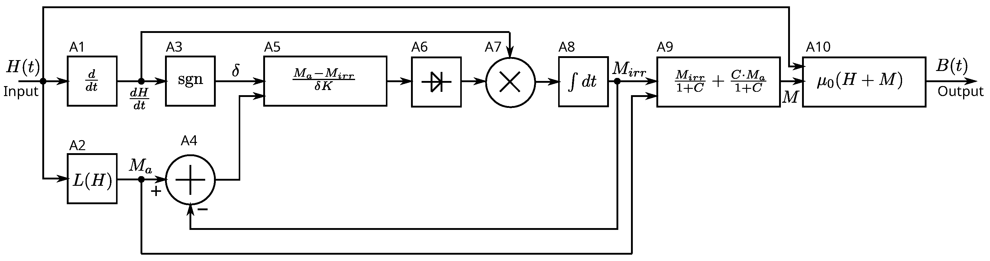
The functional block diagram explaining the equivalent circuit operation is shown in Figure 3.

Figure 3. Magnetic core model functional block diagram.

The input of the model is magnetic field strength $H\left(t\right)$, and the output is the flux density $B\left(t\right)$. The solution of the J.-A. model’s ODE is preformed by computation of the complex feedback system’s output signal. The A1 block (B4C1R1 stage in Figure 2) is a differentiation unit that computes the time derivative of the input signal. The A2 block (B5 source) computes the Langevin function, which reflects the anhysteric magnetization $M_a$. The A3 block computes the sign of the magnetic field strength’s time derivative (parameter $\delta$). The A4 block computes the difference between anhysteric and irreversible $M_{irr}$ magnetization. The A5 block (B8 source) computes Equation (5). The A6 block is an ideal rectifier stage. The A6 and A7 blocks (B7C2 circuit in Figure 2) perform the numeric integration over time and compute the $M_{irr}$. The A9 block (B2 source) computes the total magnetization M. Finally, the A10 block computes the value of magnetic flux density B.

2.3. Winding Equivalent Circuit

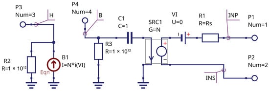
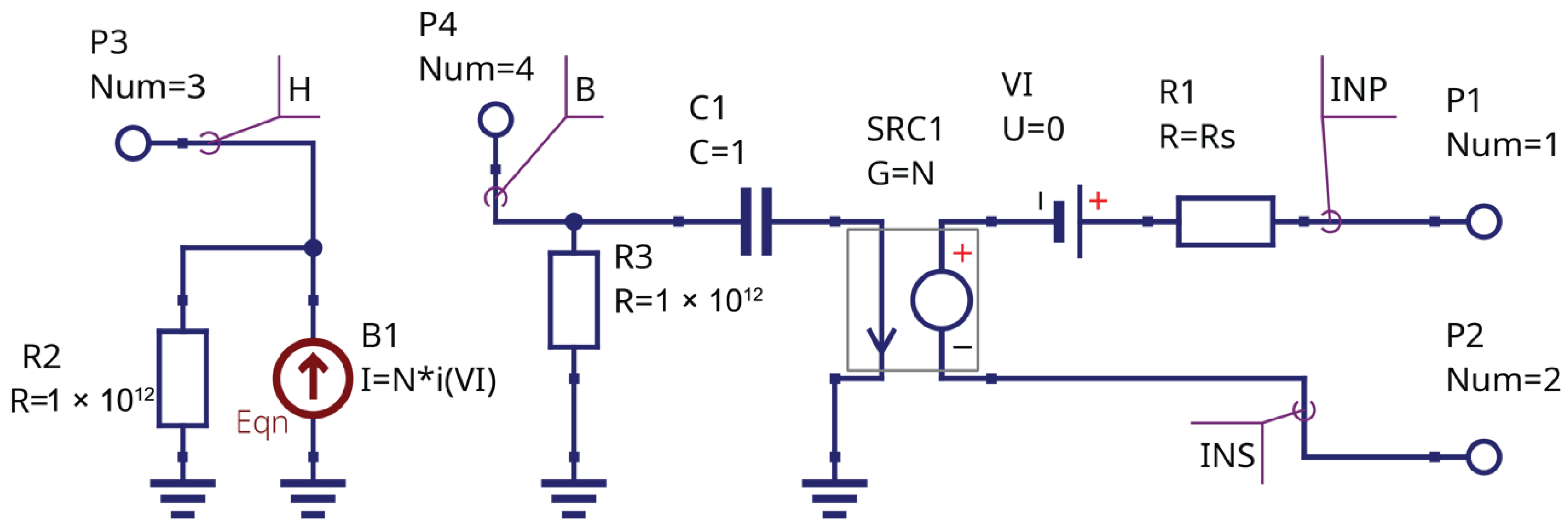
The equivalent schematic of the winding is shown in Figure 4.

Figure 4. Winding equivalent circuit.

The winding has four terminals: the pair INP and INS represent the physical connection of the transformer winding, and the other two terminals should be connected to the virtual magnetic field input and flux output of the core model (Figure 1). It is allowed to connect multiple windings to one core because the magnetic flux is represented as the virtual voltage, and the magnetic field strength is represented as the virtual current. This makes the proposed models flexible and modular. The source B1 represents the magnetic field strength H and is connected to terminals marked by the letter H; its equation is as follows:

$$H\left(t\right)={\displaystyle \frac{NI\left(t\right)}{L}}$$

(10)

where N is the winding turn number, I is the winding current, and L is the magnetic path length.

The current-controlled voltage source (CCVS) SRC1, capacitor C1, and resistor R1 represent the voltage equation at the winding terminals as follows:

$$V={\displaystyle \frac{d}{dt}}N\mathsf{\Phi }\left(t\right)+R_{s}I\left(t\right)$$

(11)

where $R_s$ is the winding resistance.

The SRC1 source is connected to magnetic flux terminals (node B) and winding terminals (nodes INP, INS). The source VI is the current sensor. Resistors R2 and R3 are the convergence helpers and provide a DC path to ground. The winding macromodel instance is characterized by two parameters: number of turns N and series resistance $R_s$.

2.4. Transformer Simulation

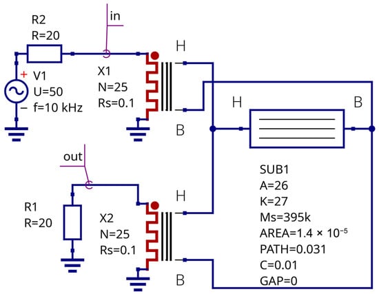
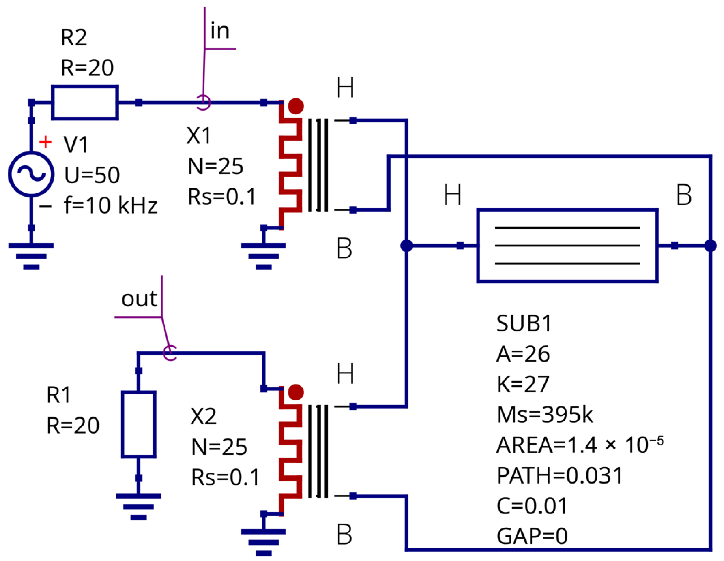
Figure 5 shows the construction of a modular transformer using the developed core and winding model. This transformer consists of two windings placed on a soft ferrite core. The core material parameters for the J.-A. model were taken from MicroCAP circuit simulator libraries. The circuit was designed using Qucs-S simulator [33,34].

Figure 5. Modular transformer schematic using proposed core and winding macromodels.

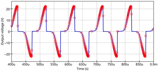
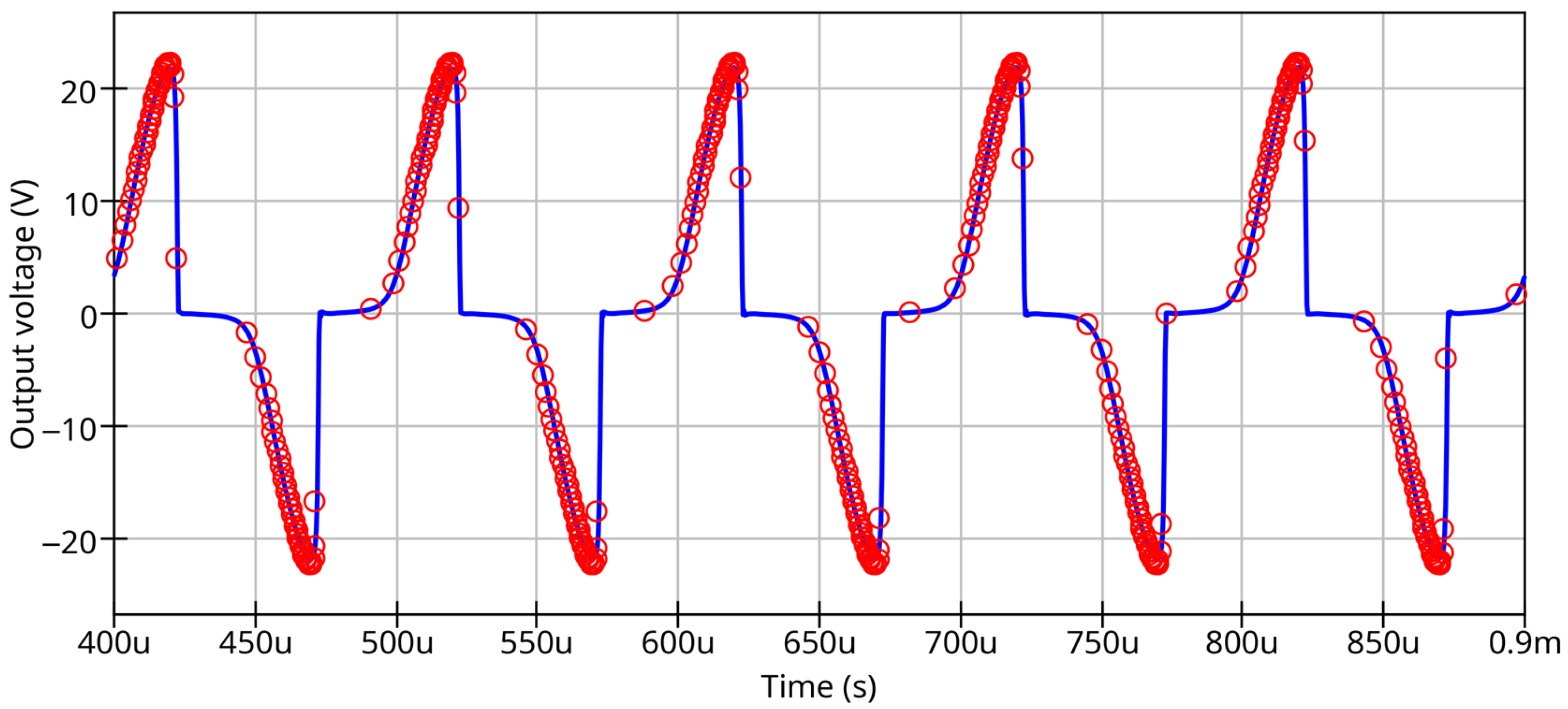
Transient simulation results for the transformer are shown in Figure 6. The developed magnetic core macromodel was simulated using the Qucs-S tool with the Ngspice backend. The MicroCAP circuit simulator was used as a reference.

Figure 6. Transformer output voltage waveform simulated with Qucs-S (solid curve), and MicroCAP reference data (circles).

The proposed approach allows for the construction of transformer models of any complexity or schematics of a single inductance with a ferromagnetic coil. The simulation results from MicroCAP and Qucs-S with the Ngspice backend using the proposed core and winding models are identical. This result shows that the developed ferromagnetic core macromodel could be used as an open-source replacement for proprietary models and allows for the reuse of the existing model parameter databases. The designed core and winding models can be exported to Verilog-A form using an automatic Verilog-A synthesizer [35] and compiled for Ngspice using the OpenVAF compiler [36].

Nevertheless, both the MicroCAP model and the open magnetic core model designed by the author share a common weak point: both models show a bad match with experimental data when the core does not reach saturation, and both show a false saturation for minor hysteresis loops. It is necessary to develop an improved version of the J.-A. model to resolve this issue.

3. Improved Jiles–Atherton Magnetic Hysteresis Model

3.1. Equation Modifications

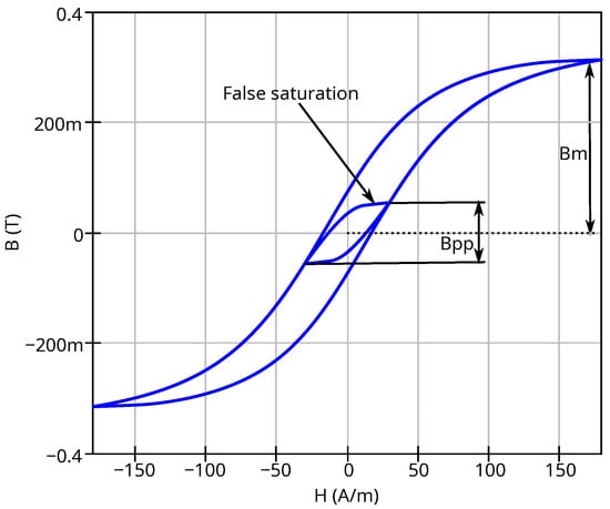
Figure 7 illustrates the problem with false saturation at low excitation levels if the peak-to-peak value of magnetic flux density $B_{pp}$ does not reach the saturation flux density $B_m$. This may lead to incorrect simulation results for low transient signals.

Figure 7. False saturation of magnetic core represented by unmodified J.-A. model at low excitation.

The minor hysteresis loops may be matched with experimental data by applying variation to the J.-A. model parameters A, K, and C (see Section 2.1). Ref. [30] proposes introducing a power-law dependency on magnetic flux density difference $B_{pp}$ at the hysteresis loop tips (peak-to-peak value) for parameters A and K, as follows:

$$K_{minor}=\eta K_{major}{\left({\displaystyle \frac{B_{pp}}{B_m}}\right)}^{\zeta }$$

(12)

$$A_{minor}=\lambda A_{major}{\left({\displaystyle \frac{B_{pp}}{B_m}}\right)}^{\xi }$$

(13)

where $A_{major}$ and $K_{major}$ are the values for A and K extracted for major hysteresis loops, respectively, while $\eta$, $\lambda$, $\zeta$, and $\xi$ are the fitting coefficients.

Ref. [32] proposes only to restrict parameter K by adding dependency on $B_{pp}$. Adding dependency of parameters A, K, and C on $B_{pp}$ implies the introduction and extraction of additional model parameters.

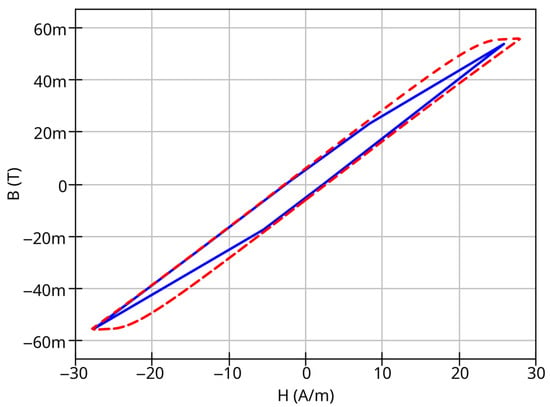
The approach proposed in [30] has the following disadvantages: It recommends a negative fitting coefficient $\xi <0$ and positive fitting coefficient $\zeta >0$. This may yield near-infinite A values and zero K values for zero excitation amplitude. This condition may take place at the initial time step for SPICE-type transient analysis. If the modified J.-A. model proposed in [30] is implemented in form of an equivalent circuit, this may lead to SPICE convergence errors. The approach proposed in [30] shows a good match of measurement data for steel-based magnetic materials, but it may show mismatch for other materials. Figure 8 shows an example of such mismatch using open-access hysteresis loop family measurement data [37].

Figure 8. Measured (solid line) and simulated (dashed line) minor hysteresis loops using variations in A and K parameters; see text for explanations.

The model parameters for major loops are as follows: $A=30.0$ A/m, $K=19.9$ A/m. The model parameters for minor loops obtained using curve fitting are $A=42.8$ A/m and $K=2.9$ A/m. It can be seen that varying the parameters A and K provides a good match for loop inclination angle and X-axis interception points, but there is a visible mismatch for minor loop shape and area, which may lead to incorrect waveform simulation results. Varying only parameter K, as proposed in [32], does not provide good matching for the minor loop inclination angle.

After the testing of the both approaches from [30] and [32], we can conclude that adding the dependency of parameter C on $B_{pp}$ gives the best match between measured minor hysteresis loop shapes and those simulated with SPICE. We propose the following dependency:

$$C\left(B_{pp}\right)=C_{major}+C_{minor}exp(-{\gamma }_C{B}_{pp}/B_m)$$

(14)

where $C_{major}$ is the C parameter for major loops, numerically equal to the C parameter value of the unmodified J.-A. model. $C_{minor}$ is the addition to the C parameter for minor loops when the $B_{pp}$ value is near zero. The value of $B_{pp}$ never exceeds the magnetic flux density at saturation $B_m$. If $C_{minor}=0$, the model modification is not applied. The parameter ${\gamma }_C$ is the fitting coefficient. All three mentioned parameters ($C_{major}$, $C_{minor}$, and ${\gamma }_C$) are dimensionless.

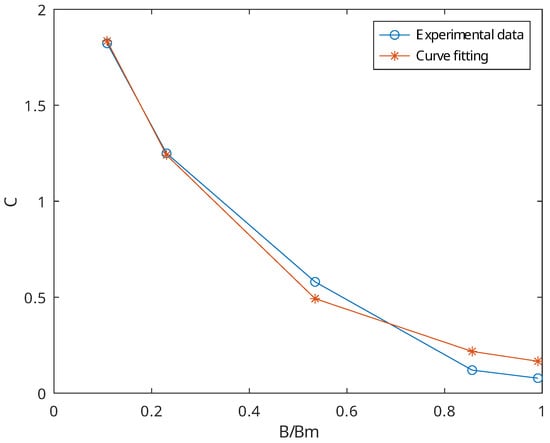
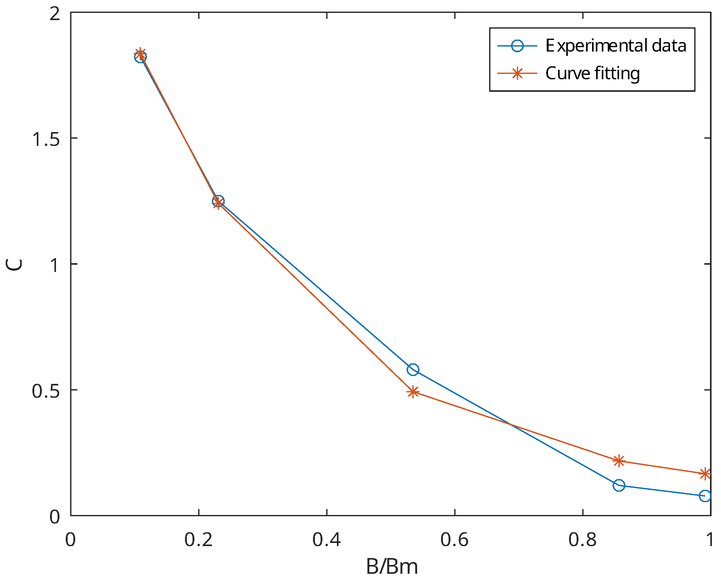
Figure 9 shows the typical dependency of C on the flux density amplitude $B_{pp}$ at the hysteresis loop tips. This dependency was extracted using the open-access hysteresis loop family measurement data [37].

Figure 9. Magnetization reversibility and C dependency fitting.

It was shown that applying the dependency only on C provides a satisfactory match of the simulations and measurements for the minor loops. If this match is not sufficient, the dependency of A on $B_{pp}$ may be added as follows:

$$A\left(B_{pp}\right)=A_{major}(1+{\beta }_{A}exp(-{\gamma }_A{B}_{pp}/B_m))$$

(15)

where ${\beta }_A$ and ${\gamma }_A$ are dimensionless fitting coefficients. Setting ${\beta }_A=0$ allows us to disable the dependency of A on $B_{pp}$. Setting both additional parameters $C_{minor}$ and ${\beta }_A$ to zero provides backward compatibility of the improved J.-A. model with the basic model version. The proposed dependencies for parameters A and C both have no discontinuities near zero and provide a better model robustness for SPICE implementation.

3.2. Equivalent Circuit of the Improved Model

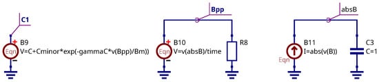
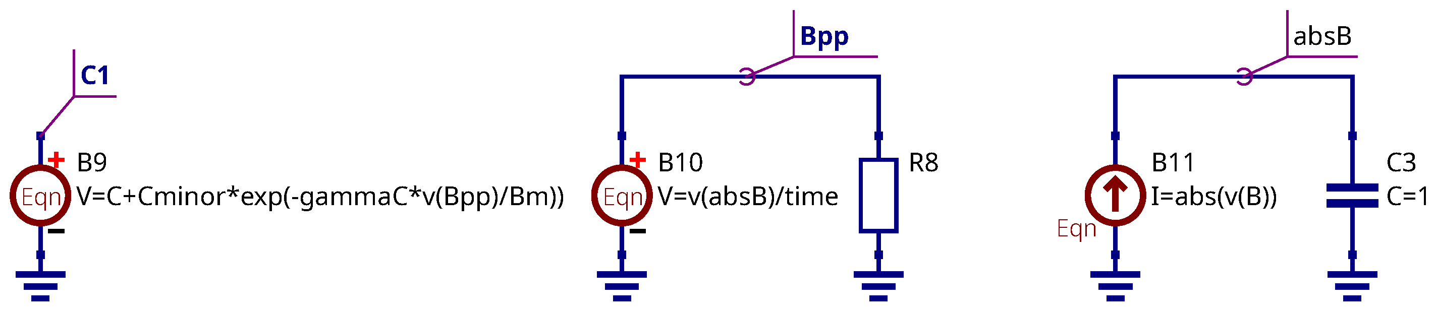
Let us consider an equivalent circuit implementation of the improved model. It is necessary to add three controlled sources to the schematics shown in Figure 1 and Figure 2. The additional elements are shown in Figure 10. The enumeration of the components continues that shown in Figure 2.

Figure 10. Modification of the core equivalent schematic.

Two controlled sources, B10 and B11, represent the ideal full-wave rectifier with an ideal ripple filter. This circuit may be replaced by an ideal diode bridge with ideal ripple filter connected to its output. The virtual output voltage at node Bpp represents the rectified averaging amplitude indicator. This value serves to introduce the dependency of the model parameters on the peak-to-peak magnetic flux density value at the BH loop tips because SPICE does not provide a direct method for peak-to-peak value extraction. The $B_{pp}$ value is determined for transient simulation time point $T_{sim}$ as follows:

$$B_{pp}\left(T_{sim}\right)={\displaystyle \frac{1}{T_{sim}}}\underset{0}{\overset{T_{sim}}{\int }}\left|B\left(t\right)\right|dt$$

(16)

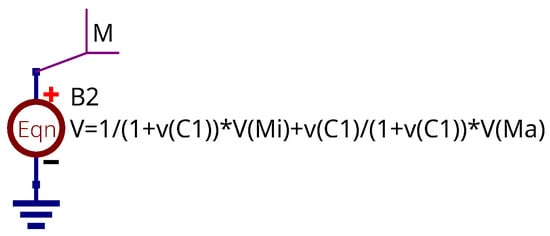
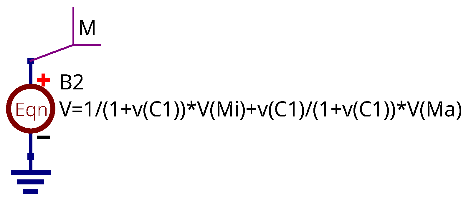
The controlled source B9 produces a virtual voltage at the node labeled with the marker C1. This voltage represents the C model parameter’s dependency on $B_{pp}$ given in Equation (14). The controlled source B2 from Figure 1 should be modified as shown in Figure 11:

Figure 11. Modification of controlled source B2.

The dependency of parameter A on the peak-to-peak magnetic flux density value could be added using a similar approach to the voltage source. In this case, parameter A in the B5 source equation (Figure 2) should be replaced by virtual voltage.

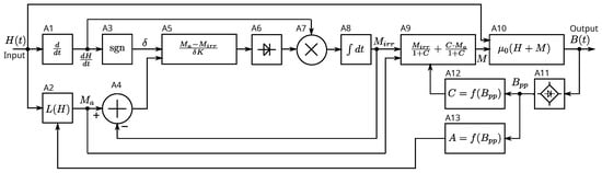
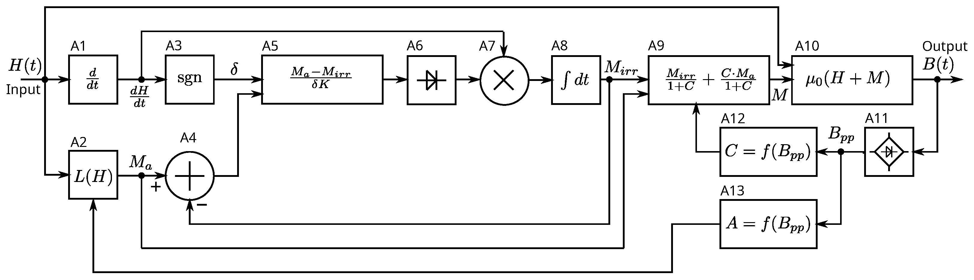
The modified block diagram of the improved model is shown in Figure 12; it has three new blocks added: A11 is an ideal full-wave rectifier serving to obtain the $B_{pp}$ value, while the blocks A12 and A13 add the dependency of parameters C and A on $B_{pp}$. The block A13 could be excluded for the simplified version of the model.

Figure 12. Improved magnetic core model functional block diagram.

4. Improved Model Verification

4.1. Measured and Simulated Ferrite Core Hysteresis Loops

The hysteresis loops for soft ferrite samples were measured to verify the modified J.-A. model. We used our own measurement data, along with open-access measurement data. The following ferrites were selected:

• Epcos N87 (measured by the author);
• Amidon 43 (measured by the author);
• Ferroxcube 3C85 (measurement data provided in [38]);
• Unnamed ferrite ring #1 (measured by the author);
• Unnamed ferrite ring #2 (measurement data provided in [37]).

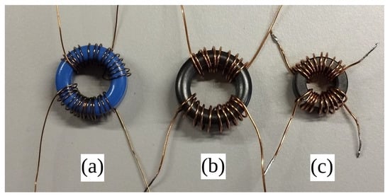
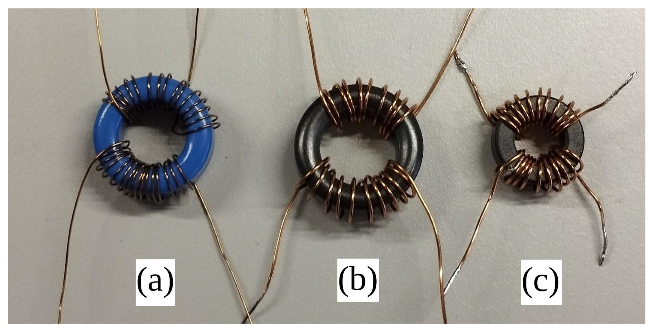
All tested ferrite samples were in the form of ring cores. A photo of the tested ferrite rings samples is shown in Figure 13.

Figure 13. Tested ferrite ring samples: Epcos N87 (a); unnamed ring #1 (b); Amidon 43 (c).

The modified J.-A. model parameters for all measured ferrites are summarized in Table 1. These parameters were obtained via manual curve fitting using the parameter tuner tool of the Qucs-S application. The general extraction procedure involved the following steps:

Table 1. J.-A. model parameters for measured ferrite core samples.

Parameter	Epcos N87	Ferroxcube 3C85	Amidon 43	No Name #1	No Name #2
A (A/m)	12.3	28.5	12.0	12.0	30.0
K (A/m)	18.3	16.7	39.1	38.0	19.9
$M_s$ (A/m)	$3.95\times {10}^5$	$4.27\times {10}^5$	$2.33\times {10}^5$	$2.20\times {10}^5$	$2.30\times {10}^5$
$C=C_{major}$	0.14	0.1	0.04	0.37	0.08
$\alpha$	${10}^{-4}$	${10}^{-4}$	${10}^{-4}$	${10}^{-4}$	${10}^{-4}$
$C_{minor}$	1.15	1.6	1.0	0.2	2.0
${\gamma }_C$	2.7	2.3	3.0	3.0	3.0
${\beta }_A$	1.2	0.40	0	0	0
${\gamma }_A$	4.0	3.0	-	-	-

1.

Compute the initial saturation magnetization parameter $M_s$, which uses the saturation flux density $B_s$ of the major hysteresis loop as follows: $M_s={10}^6·B_s$. Set the initial values ${\beta }_A=0$, $C_{minor}=0$, and ${\gamma }_A={\gamma }_C=3.0$.

2.

Tune A parameter to match the loop inclination.

3.

Tune K parameter to match the loop interception points on the X-axis (coercitivity).

4.

Tune $C_{major}$ and $\alpha$ parameters to match the loop interception points on the Y-axis (residual flux density).

5.

Repeat Steps 2–4 to achieve the best matching of the measured and simulated major hysteresis loop forms.

6.

Start to increase the $C_{minor}$ value to match the form of the minor hysteresis loops. This could also be adjusted using the ${\gamma }_C$ coefficient.

7.

If the minor loop form matching was not achieved using only $C_{minor}$, increase ${\beta }_A$ and adjust ${\gamma }_A$ to achieve the best matching.

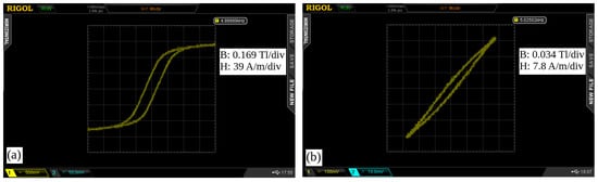
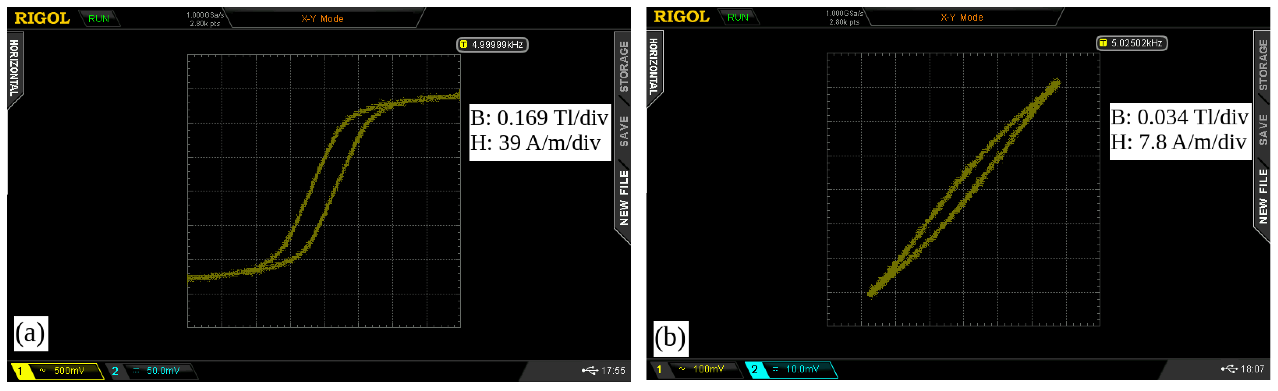
Figure 14 shows the raw hysteresis loop measurement data for the N87 ferrite sample. The screenshots were taken from the digital oscilloscope. The horizontal axis (Channel 1) represents magnetic field strength, and the vertical axis (channel 2) represents flux density. The measurements were taken using a schematic containing a sinusoidal waveform generator, amplifying module, and analog integrator [28,39]. The measurement setup is trivial, and its schematic is not provided here.

Figure 14. Measured major (a) and minor (b) hysteresis loops for N87 ferrite.

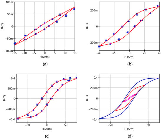
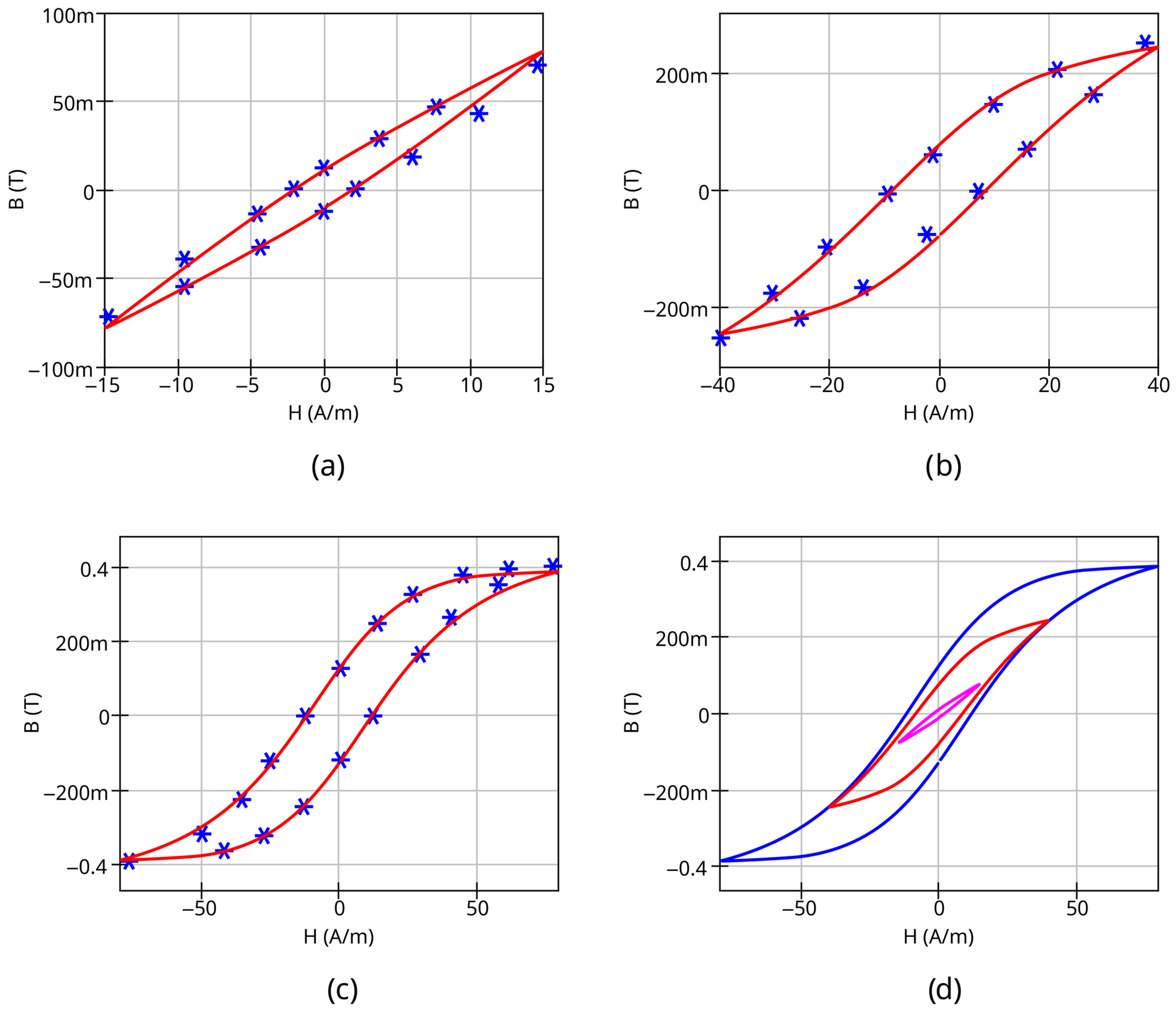
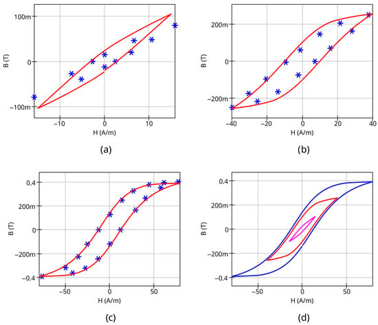
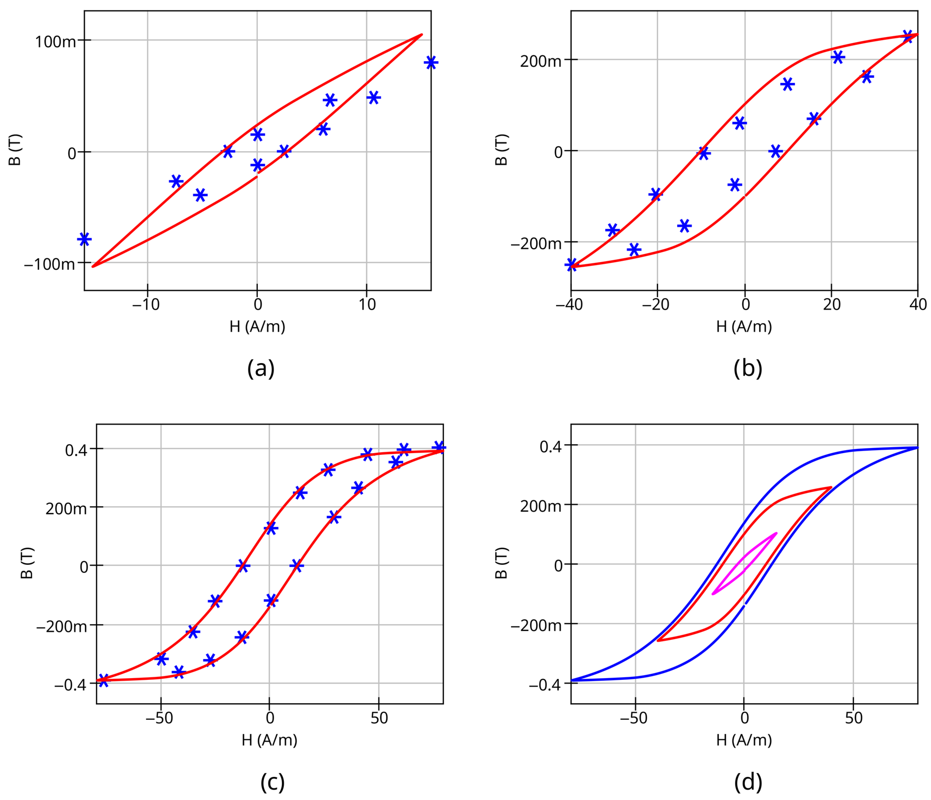
The simulation results for the family of hysteresis loops, compared with measurement data for Epcos N87 ferrite, are shown in Figure 15. The dependency on the peak-to-peak magnetic flux density value was applied for parameters A and C for the simulation (set $C_{minor}>0$ and ${\beta }_A>0$). A similar comparison for the other ferrites can be found in the Data Availability Statement Section.

Figure 15. Comparison of measured (stars) and simulated (solid curve) hysteresis loops for different magnetic field strength H amplitudes: 15 A/m (a), 30 A/m (b), and 100 A/m (c). Family of simulated hysteresis curves (d). EPCOS N87 ferrite; $C_{minor}=1.15$; ${\beta }_A=1.2$.

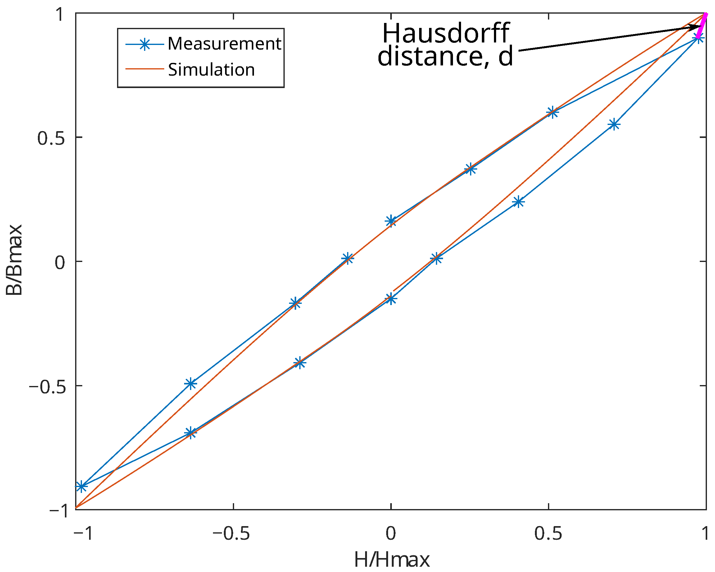
The Hausdorff normalized distance [40] and hysteresis loop area can be used as a numeric measure to compare the simulated and measured hysteresis loops. The Hausdorff distance [41] is defined as the maximum distance between any point on the first set and its nearest point on the second set, and vice versa. The combination of these two parameters allows for the numerical comparison of the arbitrary curves’ shape. The hysteresis loops were normalized in $B/B_{pp}$ and $H/H_{pp}$ coordinates, and then the Hausdorff distance between the most distant points of the simulated and measured hysteresis loops was calculated. The area mismatch $\Delta A$ was calculated as follows:

$$\Delta A={\displaystyle \frac{|A_{sim}-A_{meas}|}{A_{meas}}}·100\%$$

(17)

where $A_{sim}$ and $A_{meas}$ are the area of the simulated and measured hysteresis loops, respectively.

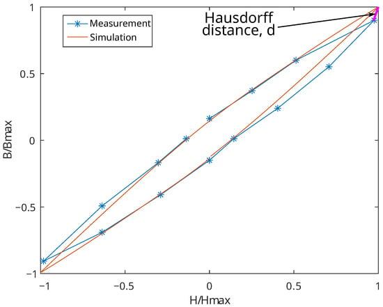
Figure 16 illustrates the normalization and comparison process performed using the GNU Octave [42] numeric mathematics package; it shows the computation of the Hausdorff distance between the simulated and measured loops for the most inner loop from Figure 15d.

Figure 16. Hausdorff distance (bold magenta line) computation for the measured and simulated minor hysteresis loops.

The most distant points of the simulated and measured loops are located on the loop tips. The results for all three loops (inner, middle, and outer), as shown in Figure 15, are compared in Table 2. It can be seen that the mismatch increases for the minor loops but remains within satisfactory limits.

Table 2. The numeric comparison of simulated and measured hysteresis loops.

Hysteresis Loop (Figure 15d)	Hausdorff Distance, d (Dimensionless)	Area Mismatch, $\mathbf{\Delta }\mathit{A}$ (%)
Outer	0.045	3.6
Middle	0.066	5.6
Inner	0.105	13

Figure 17 shows the measured and simulated hysteresis loops for N87 ferrite if only dependency for C is applied and the ${\beta }_A$ coefficient is set to zero. This is a simplified variant of the proposed model.

Figure 17. Comparison of measured (stars) and simulated (solid curve) hysteresis loops for different magnetic field strength H amplitudes: 15 A/m (a), 30 A/m (b), and 100 A/m (c). Family of simulated hysteresis curves (d). EPCOS N87 ferrite; $C_{minor}=1.15$; ${\beta }_A=0$.

It can be seen that there is significant mismatch for the smallest minor loop. This mismatch could be estimated as more than 30% using the Hausdorff metrics and area comparison. However, the model without ${\beta }_A$ and ${\gamma }_A$ coefficients still shows a satisfactory transient simulation match, as shown in this section. Moreover, this simplification may be accepted despite the remaining mismatch because of the more simple extraction procedure. This form of the modified J.-A. model requires the fitting of two additional parameters instead of four. The variant using ${\beta }_A=0$ could be used if additional measurements of minor loops are not available because for most soft ferrites it is sufficient to set $C_{minor}$ in a range from 1.0 to 2.0 and ${\gamma }_C$ in a range from 2.0 to 3.0 (see Table 1). The unnamed sample #1 from Table 1 with $C_{minor}=0.2$ has a different hysteresis loop form, characterized by a high residual flux density. This explains the large difference in its extracted $C_{minor}$ value compared with other measured samples.

4.2. Comparison of Simulated and Measured Output Waveforms for Ferrite Core Transformer Circuit

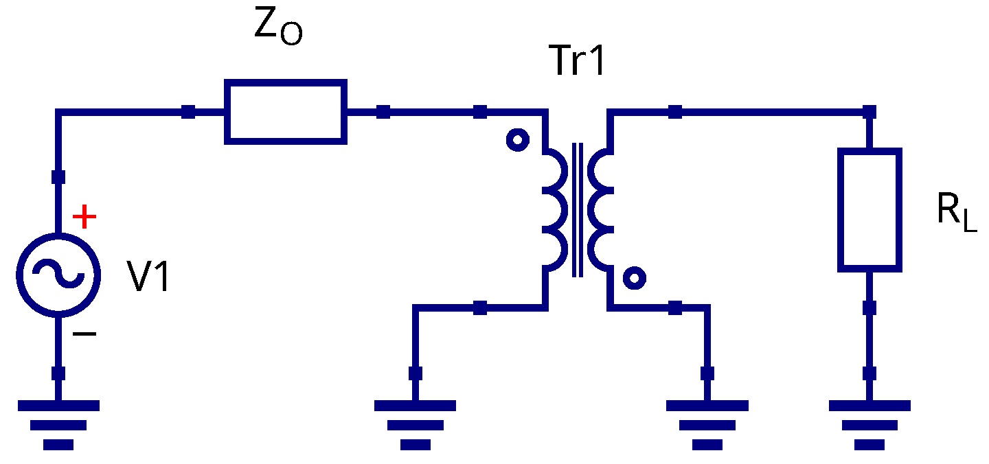
The test schematic is shown in Figure 18. The source V1 represents the waveform generator, and the $Z_O$ resistor is its output impedance. The Tr1 component is a 1:1 transformer wound on the tested ferrite core. The primary transformer winding is connected to generator, and the secondary winding is connected to resistive load $R_L$. The output impedance of the used waveform generator is $Z_O=50$ Ohms. The load resistance was set to 220 Ohms. The waveform at the transformer’s secondary winding terminals could be controlled by an oscilloscope. in the schematic.

Figure 18. Test schematic for comparison of simulated and measured waveforms; see text for explanation.

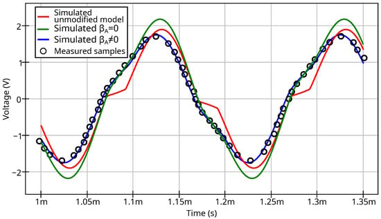
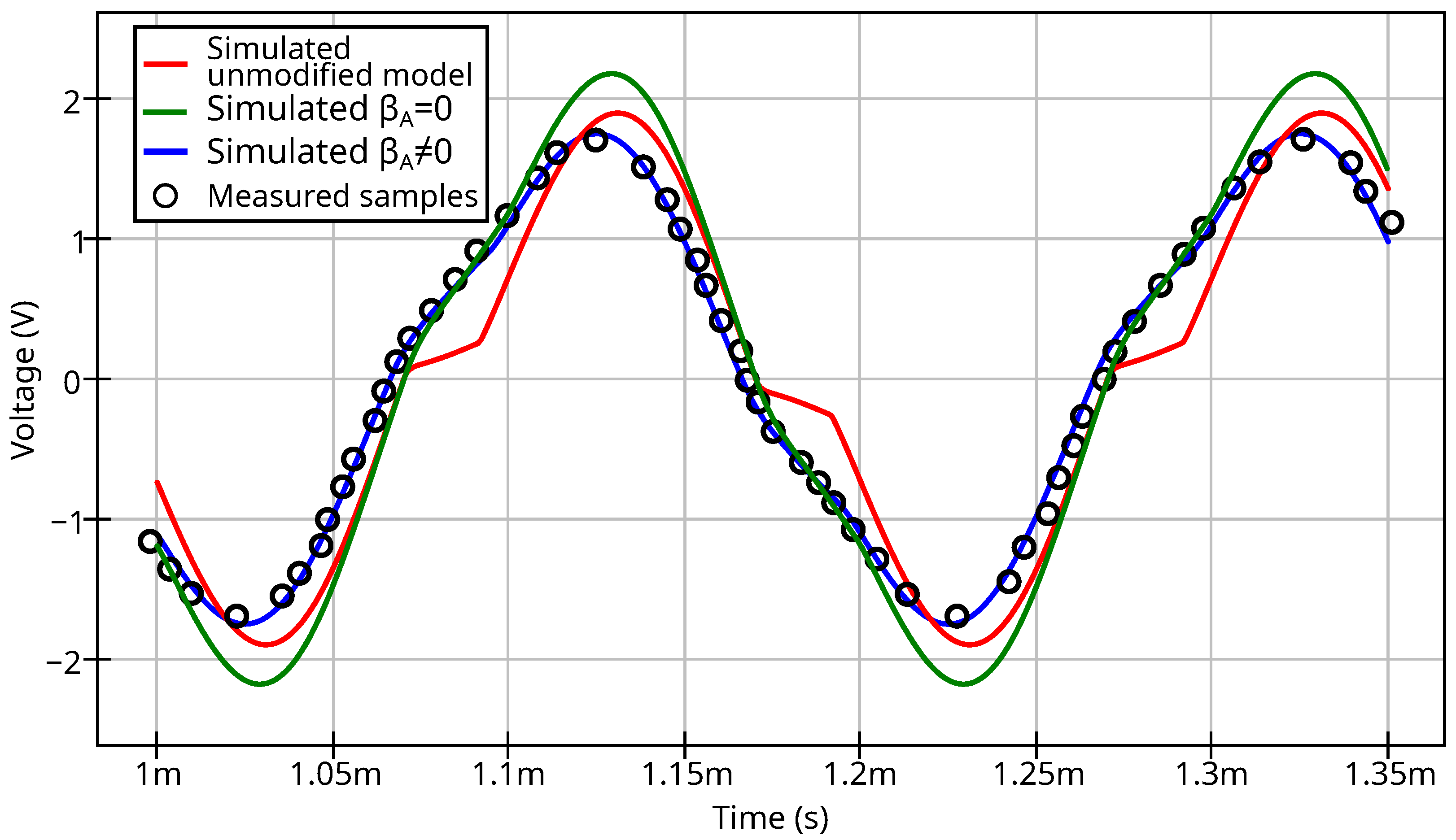
The simulated and measured waveforms for the transformer with an N87 ferrite ring core are shown in Figure 19. The core parameters are as follows: outer diameter 16.5 mm, inner diameter 9.6mm, and height 6.3 mm. Both the primary and secondary windings have 15 turns of AWG29 copper wire.

Figure 19. Simulated and measured waveforms for ferrite core transformer circuit; see legend for explanation.

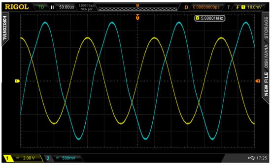
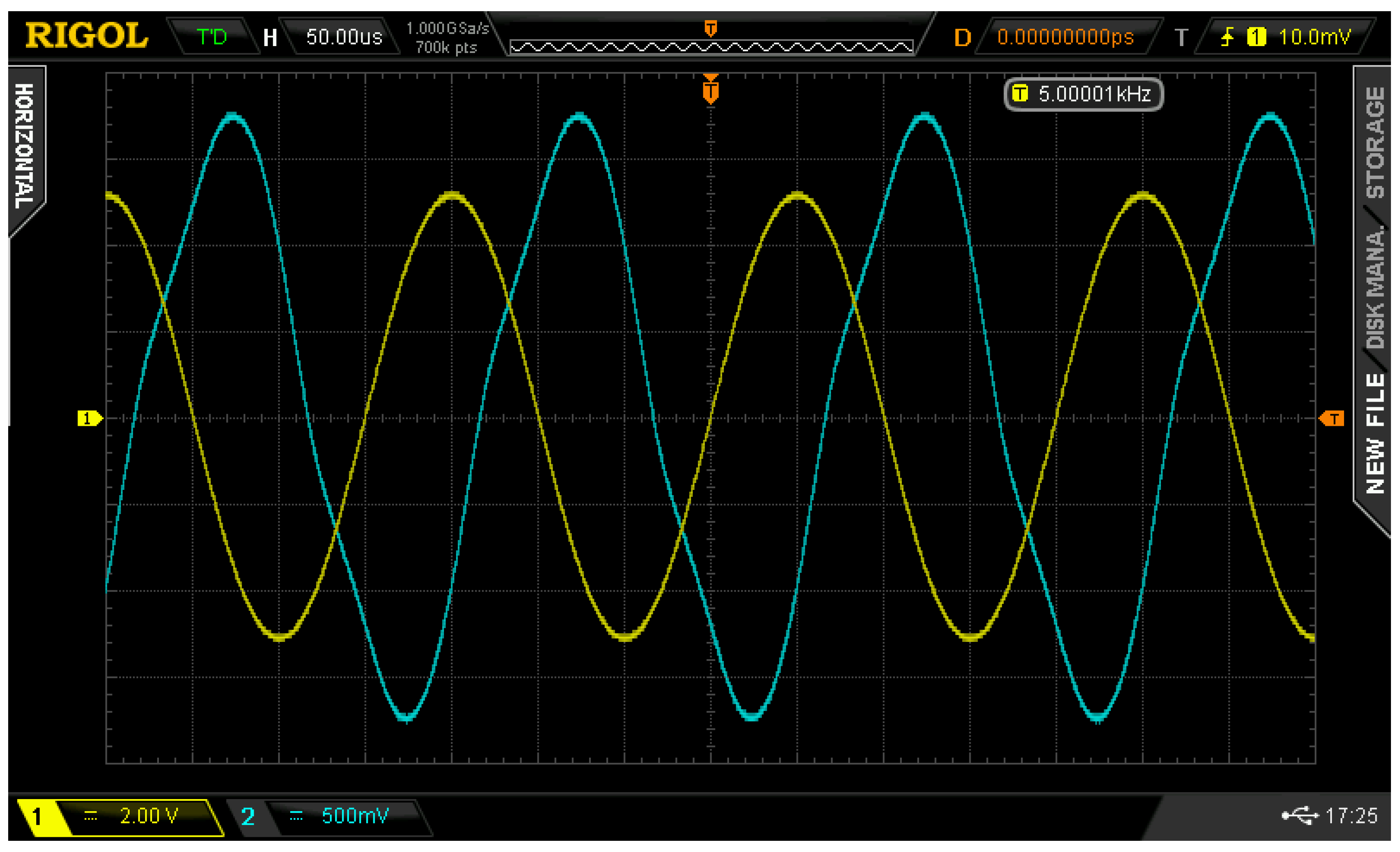
The raw measured waveform at the transformer output (oscilloscope screenshot) is shown in Figure 20.

Figure 20. Measured waveforms at the generator output (yellow trace) and N87 core transformer output (blue trace).

It can be seen that the unmodified J.-A. model shows a step when crossing zero. The simulated output waveform of the transformer using the modified core model has a good match with the measured waveform. If the modified model uses only two additional parameters (set ${\beta }_A=0$), the waveform will still not be distorted; however, a difference appears in the peak-to-peak output voltage value. The waveform plots show that both variants of the modified J.-A. model eliminate the step at zero crossing and false saturation at minor loops. The variant using only two additional parameters may be preferable because of its more easy parameter extraction procedure.

The measured and simulated normalized harmonics levels (amplitude spectrum) of the transformer output voltage are shown in Table 3. The test schematic and conditions are as shown in Figure 18. The fundamental frequency is 5 kHz, and the input signal amplitude is 5 V. Table 3 shows only the 3th, 5th, and 7th harmonics because the even harmonics have near zero level, and the harmonics above the 7th are below the measurement equipment’s resolution. The magnitude of the first harmonic is normalized to a value of 1.0. The unmodified J.-A. model is not included in Table 3 because its waveform difference is obvious.

Table 3. Simulated and measured normalized spectra of transformer output voltage.

Harmonic Number	Simulated ${\mathit{\beta }}_{\mathit{A}}\ne 0$	Simulated ${\mathit{\beta }}_{\mathit{A}}=0$	Measured
1	1.0	1.0	1.0
3	0.115	0.116	0.096
5	0.019	0.017	0.017
7	0.002	0.003	0.002

Table 4 compares the simulated and measured time-domain data numerically. The values of root-mean-square error (RMSE) and normalized root-mean-square error (NRMSE) were used as metrics of waveform similarity. The measured and simulated waveforms were normalized to the amplitude before computing the NRMSE, allowing for the estimation of the waveforms’ shape deviation from the measured values.

Table 4. The numerical comparison of simulated and measured waveforms.

Waveform	RMSE (mV)	NRMSE (%)
Simulated ${\beta }_A=0$	340	8.9
Simulated ${\beta }_A\ne 0$	65	3.9

The model using ${\beta }_A\ne 0$ achieves a good match between the simulated and measured data, with a simulation error within 5%. The model using ${\beta }_A=0$ (two additional parameters) has a significant absolute RMSE of 340 mV for a signal amplitude of 1.70 V, but it still reproduces the measured waveform shape (see Table 3 for the spectrum and NRMSE value). Therefore, the variant with two parameters could be used for signal distortion estimation despite the mismatch in amplitude value.

5. Conclusions

An improved J.-A. magnetic hysteresis model and its SPICE implementation are presented in this study. The advantage of the proposed model modification is that it not only provides modified equations but also considers integration with SPICE simulation software. The modified model provides better experimental data matching for soft ferrite materials. The improved J.-A. model is backward compatible with the basic version used in proprietary circuit simulation software and requires the extraction of two or four additional parameters. Using the improved model eliminates the problem of false saturation when simulating transformers at low excitation. The developed ferromagnetic core model is fully compatible with open-source SPICE implementations such as Ngspice. The proposed J.-A. model with extensions demonstrates a good match between simulated and measured results, as illustrated by the measurement of hysteresis loops and transient waveforms. The verification was carried out only for ferrite cores, but it could be expanded to other soft magnetic materials. Combined with the SPICE winding model, this allows for the simulation of schematics containing transformers with saturated cores and achieving better performance than proprietary implementations of the J.-A. model. The extraction of additional model parameters requires the measurement of at least three hysteresis loops for different excitation levels. If the additional measurements are not available, the simplified variant with two extra parameters could be used. Both variants allow for the estimation of the signal distortion in schematics utilizing ferrite-core transformers.

The presented improved J.-A. model does not take into account effects such as the eddy current, temperature dependency of core parameters, and frequency dependency of core losses. The usage of the proposed model for steel cores and materials with high residual flux density is not covered in this research. On the other hand, the ferromagnetic core models provided by the proprietary circuit simulation software also do not take into the account the aforementioned effects, and these restrictions cannot be considered as limiting factors in the practical usage of the proposed model. Adding the aforementioned extensions to the model may become a basis for future work.

References

- Vladirmirescu, A. Shaping the History of SPICE. IEEE Solid-State Circuits Mag. 2011, 3, 36–39. [Google Scholar] [CrossRef] [Scilit]
- Brinson, M.; Tomaszewski, D. Advances in Qucs-S Schematic Capture for SPICE and Verilog-A Device Modelling and Circuit Simulation. In 2022 29th International Conference on Mixed Design of Integrated Circuits and System (MIXDES); IEEE: Piscataway, NJ, USA, 2022; pp. 27–32. [Google Scholar] [CrossRef] [Scilit]
- Rashid, M. SPICE and LTspice for Power Electronics and Electric Power, 4th ed.; CRC Press: Boca Raton, FL, USA, 2024. [Google Scholar] [CrossRef] [Scilit]
- Górecki, K.; Detka, K. SPICE-Aided Models of Magnetic Elements—A Critical Review. Energies 2023, 16, 6568. [Google Scholar] [CrossRef] [Scilit]
- Górecki, K.; Górski, K. SPICE-Aided Compact Electrothermal Model of Impulse Transformers. Appl. Sci. 2021, 11, 8894. [Google Scholar] [CrossRef] [Scilit]
- Salas, R.; Pleite, J.; Olías, E.; Barrado, A. Theoretical–experimental comparison of a modeling procedure for magnetic components using finite element analysis and a circuit simulator. J. Magn. Magn. Mater. 2008, 320, e1024–e1028. [Google Scholar] [CrossRef] [Scilit]
- Kelp, K.; Wright, D.; Stephens, J.; Dickens, J.; Mankowski, J.; Shaw, Z.; Neuber, A. Modeling Pulsed Magnetic Core Behavior in LTspice. Electronics 2025, 14, 2335. [Google Scholar] [CrossRef] [Scilit]
- Saeed, S.; Georgious, R.; Garcia, J. Modeling of Magnetic Elements Including Losses—Application to Variable Inductor. Energies 2020, 13, 1865. [Google Scholar] [CrossRef] [Scilit]
- Knežević, P.; Radaković, A.; Velimirović, N.; Čukanović, D.; Perović, Z.; Radulović, R.; Bogdanović, G. A Preisach Model Defining Correlation Between Monotonic and Cyclic Response of Structural Mild Steel. Mathematics 2024, 12, 3330. [Google Scholar] [CrossRef] [Scilit]
- Chan, J.; Vladimirescu, A.; Gao, X.C.; Liebmann, P.; Valainis, J. Nonlinear transformer model for circuit simulation. IEEE Trans.-Comput. Des. Integr. Circuits Syst. 1991, 10, 476–482. [Google Scholar] [CrossRef] [Scilit]
- Fallahnejad, M.; Afrakhte, H. The comparison of two approaches Jiles-Atherton and Preisach in simulating hysteresis cycle. In 2015 2nd International Conference on Knowledge-Based Engineering and Innovation (KBEI); IEEE: Piscataway, NJ, USA, 2015; pp. 710–713. [Google Scholar] [CrossRef] [Scilit]
- Khemani, V.; Azarian, M.H.; Pecht, M.G. Efficient Identification of Jiles–Atherton Model Parameters Using Space-Filling Designs and Genetic Algorithms. Eng 2022, 3, 364–372. [Google Scholar] [CrossRef] [Scilit]
- Szewczyk, R.; Cheng, P. Open Source Implementation of Different Variants of Jiles-Atherton Model of Magnetic Hysteresis Loops. Acta Phys. Pol. A 2018, 133, 654–656. [Google Scholar] [CrossRef] [Scilit]
- Scorretti, R.; Sixdenier, F. An analytical formula to identify the parameters of the energy-based hysteresis model. J. Magn. Magn. Mater. 2022, 548, 168748. [Google Scholar] [CrossRef] [Scilit]
- Kaltenbacher, M.; Roppert, K.; Domenig, L.D.; Egger, H. Comparison of Energy Based Hysteresis Models. In 2022 23rd International Conference on the Computation of Electromagnetic Fields (COMPUMAG); IEEE: Piscataway, NJ, USA, 2022; pp. 1–4. [Google Scholar] [CrossRef] [Scilit]
- Frydrych, P.; Szewczyk, R. Preisach Based Model for Predicting of Functional Characteristic of Fluxgate Sensors and Inductive Components. In Recent Advances in Automation, Robotics and Measuring Techniques; Szewczyk, R., Zieliński, C., Kaliczyńska, M., Eds.; Springer: Cham, Switzerland, 2014; pp. 591–596. [Google Scholar] [CrossRef] [Scilit]
- Wang, Z.; Hur, J.; Tasneem, N.; Chern, W.; Yu, S.; Khan, A. Extraction of Preisach model parameters for fluorite-structure ferroelectrics and antiferroelectrics. Sci. Rep. 2021, 11, 12474. [Google Scholar] [CrossRef] [Scilit] [PubMed]
- Zhai, Y.; Vu-Quoc, L. Analysis of power magnetic components with nonlinear static hysteresis: Finite-element formulation. IEEE Trans. Magn. 2005, 41, 2243–2256. [Google Scholar] [CrossRef] [Scilit]
- Willerich, S.; Herzog, H.G. A Continuous Vector Preisach Model Based on Vectorial Relay Operators. IEEE Trans. Magn. 2020, 56, 7511204. [Google Scholar] [CrossRef] [Scilit]
- Moll, D.; D’Angelo, L.A.M.; Gersem, H.D.; Boattini, F.; Bottura, L.; Gast, M. A Dynamic Energy-Based Hysteresis Model for Pulsed-Operated Fast-Ramping Magnets. IEEE Trans. Magn. 2025, early access. [Google Scholar] [CrossRef] [Scilit]
- Quondam Antonio, S.; Ghanim, A.; Faba, A.; Laudani, A. Numerical simulations of vector hysteresis processes via the Preisach model and the Energy Based Model: An application to Fe-Si laminated alloys. J. Magn. Magn. Mater. 2021, 539, 168372. [Google Scholar] [CrossRef] [Scilit]
- Bedritskiy, I.; Jurayeva, K.; Bazarov, L.; Mirasadov, M. Chan hysteresis models and magnetization curve models for cores made of soft magnetic amorphous alloys. AIP Conf. Proc. 2025, 3256, 030015. [Google Scholar] [CrossRef] [Scilit]
- Jiles, D.C.; Atherton, D.L. Theory of ferromagnetic hysteresis (invited). J. Appl. Phys. 1984, 55, 2115–2120. [Google Scholar] [CrossRef] [Scilit]
- Jiles, D.; Atherton, D. Theory of ferromagnetic hysteresis. J. Magn. Magn. Mater. 1986, 61, 48–60. [Google Scholar] [CrossRef] [Scilit]
- Regan, A.; Wilson, J.; Peyton, A.J. Extension to the Jiles–Atherton Hysteresis Model Using Gaussian Distributed Parameters for Quenched and Tempered Engineering Steels. Sensors 2025, 25, 1328. [Google Scholar] [CrossRef] [Scilit]
- Jaroszyński, L. Magnetic core model for a reliable simulation of three-phase transformer in PSPICE. In 2017 International Conference on Electromagnetic Devices and Processes in Environment Protection with Seminar Applications of Superconductors (ELMECO & AoS); IEEE: Piscataway, NJ, USA, 2017; pp. 1–4. [Google Scholar] [CrossRef] [Scilit]
- Grabinski, W.; Scholz, R.; Verley, J.; Keiter, E.R.; Vogt, H.; Warning, D.; Nenzi, P.; Lannutti, F.; Salfelder, F.; Davis, A.; et al. FOSS CAD for the Compact Verilog-A Model Standardization in Open Access PDKs. In 2024 8th IEEE Electron Devices Technology & Manufacturing Conference (EDTM); IEEE: Piscataway, NJ, USA, 2024; pp. 1–3. [Google Scholar] [CrossRef] [Scilit]
- Luo, M.; Dujic, D.; Allmeling, J. Modeling Frequency Independent Hysteresis Effects of Ferrite Core Materials Using Permeance–Capacitance Analogy for System-Level Circuit Simulations. IEEE Trans. Power Electron. 2018, 33, 10055–10070. [Google Scholar] [CrossRef]
- Xue, G.; Bai, H.; Li, T.; Lu, C. An Easily Used Phenomenological Magnetization Model and Its Empirical Expressions Based on Jiles–Atherton Parameters. Materials 2022, 15, 7592. [Google Scholar] [CrossRef] [Scilit] [PubMed]
- Chwastek, K. Modelling offset minor hysteresis loops with the modified Jiles–Atherton description. J. Phys. D Appl. Phys. 2009, 42, 165002. [Google Scholar] [CrossRef] [Scilit]
- Fulginei, F.; Salvini, A. Softcomputing for the identification of the Jiles-Atherton model parameters. IEEE Trans. Magn. 2005, 41, 1100–1108. [Google Scholar] [CrossRef] [Scilit]
- Lindner, A.; Hahn, I.; Böhm, A. A simple method for the parameter identification of the Jiles-Atherton model using only symmetric hysteresis loops. In IECON 2013—39th Annual Conference of the IEEE Industrial Electronics Society; IEEE: Piscataway, NJ, USA, 2013; pp. 2571–2577. [Google Scholar] [CrossRef] [Scilit]
- Kuznetsov, V. Microstrip Line Modeling Taking into Account Dispersion Using a General-Purpose SPICE Simulator. J. Low Power Electron. Appl. 2025, 15, 42. [Google Scholar] [CrossRef] [Scilit]
- Kuznetsov, V.; Andreev, D.; Andreev, V.; Piskunov, S.; Popov, A.I. The Compact Model Synthesis for the RADFET Device. Technologies 2025, 13, 492. [Google Scholar] [CrossRef] [Scilit]
- Brinson, M.; Kuznetsov, V. Qucs-0.0.19S: A new open-source circuit simulator and its application for hardware design. In 2016 International Siberian Conference on Control and Communications (SIBCON); IEEE: Piscataway, NJ, USA, 2016; pp. 1–5. [Google Scholar] [CrossRef] [Scilit]
- Kuthe, P.; Müller, M.; Schröter, M. VerilogAE: An Open Source Verilog-A Compiler for Compact Model Parameter Extraction. IEEE J. Electron Devices Soc. 2020, 8, 1416–1423. [Google Scholar] [CrossRef] [Scilit]
- Sheremetyev, D. Izmerenije Ferrita (The Measurement of Ferrite, In Russian). Available online: https://dmitry-shem.livejournal.com/28220.html (accessed on 1 November 2025).
- Alferink, F. Measuring the Magnetic Hysteresis. Available online: https://meettechniek.info/passive/magnetic-hysteresis.html (accessed on 1 November 2025).
- Pólik, Z.; Kuczmann, M. Measuring and control the hysteresis loop by using analog and digital integrators. J. Optoelectron. Adv. Mater. 2008, 10, 1861–1865. [Google Scholar]
- Ali, M.; Hussain, Z.; Yang, M.S. Hausdorff Distance and Similarity Measures for Single-Valued Neutrosophic Sets with Application in Multi-Criteria Decision Making. Electronics 2023, 12, 201. [Google Scholar] [CrossRef] [Scilit]
- Belogay, E.; Cabrelli, C.; Molter, U.; Shonkwiler, R. Calculating the Hausdorff distance between curves. Inf. Process. Lett. 1997, 64, 17–22. [Google Scholar] [CrossRef] [Scilit]
- Eaton, J.W. GNU Octave and reproducible research. J. Process Control 2012, 22, 1433–1438. [Google Scholar] [CrossRef] [Scilit]
Disclaimer/Publisher’s Note: The statements, opinions and data contained in all publications are solely those of the individual author(s) and contributor(s) and not of MDPI and/or the editor(s). MDPI and/or the editor(s) disclaim responsibility for any injury to people or property resulting from any ideas, methods, instructions or products referred to in the content. |
© 2026 by the author. Licensee MDPI, Basel, Switzerland. This article is an open access article distributed under the terms and conditions of the Creative Commons Attribution (CC BY) license.