An Arterial-Level Traffic Signal Coordinated Control Approach with Partial Connected Vehicle Data

Abstract

Most adaptive signal control systems rely on traffic data detected by fixed-point detectors, which suffers from characteristics of inaccuracy and latency. This study proposes a hierarchical coordinated signal control framework for arterials with asymmetric traffic, integrating traditional detector data and partial CV data. The arterial traffic operation is firstly considered, based on the traditional Webster’s model. An efficiency optimization model is then developed for the high-volume main direction traffic flow of the mainline. At last, a bandwidth maximization model is presented for the minor direction traffic. The experimental results based on VISSIM simulation scenarios demonstrate that the proposed approach performs better than the Synchro and MULTIBAND models, especially when the penetration rate of CVs is greater than 30%. In addition, as the penetration rate increases, the impact on mainline traffic is significant while the effect on arterial traffic is slight.

1. Introduction

In the urban transportation network, the arterials are primarily used for local and inter-regional transportation activities. Their traffic efficiency has significant impacts on the operation of the whole transportation system. Especially within the morning and evening rush hours on weekends, traffic demand on the arterials is relatively high, which may cause decreased traffic capacity and limited performance of the urban road network. Therefore, coordinated control measures for multiple consecutive intersections are required, for the smooth and efficient operation of arterial traffic flows. So far, the coordination control of arterial traffic has been mainly achieved through the adaptive signal control systems. Typically, the Sydney Coordinated Adaptive Traffic System (SCATS) and the Split-Cycle-Offset Optimization Technique (SCOOT) system have matured and been applied extensively both at home and abroad. Based on the real-time traffic data, the former selects the optimal signal timing plan from a pre-stored plan library [1]. The latter implements the dynamic optimization of signal cycle, split and offset online, based on traffic data collected by detectors upstream of intersections [2].

However, existing adaptive signal control systems rely on detection data obtained by traditional detectors like loop detector, which only reflects the fixed-point traffic status. This can hardly capture the spatiotemporal evolution of traffic characteristics, including the processes of queuing and dissipation. Additionally, coordination control systems adopting different optimization strategies also have inherent limitations. The performance of the SCATS depends on the scope of pre-stored schemes. Once traffic conditions exceed the preset range or unexpected traffic events occur, the system’s optimal scheme cannot adapt to the actual situation. The SCOOT system normally uses a small-step gradual optimization approach when adjusting signal timing parameters of cycle, split and offset. If confronting rapid changes in traffic demand or unexpected events, the late responses make it difficult to match traffic conditions.

With the swift advancement of wireless communication technology and intelligent connected vehicle (CV) technology, the collection of traffic data has evolved from a single-point mode with fixed detectors to a multi-source dynamic mode. In particular, CVs equipped with wireless communication devices exchange data with roadside units and other vehicles. CV data is currently the most discussed data source. Compared to traditional detector data, CV trajectory data possesses characteristics of high accuracy and real-time acquisition [3,4,5]. This data can provide not only values of macro traffic parameters but also detailed vehicle state information including position, acceleration and driving speed. Moreover, with advanced equipment, the transmission of CV data among vehicles and control facilities can achieve second or even sub-second precision. Given these advantages in capturing traffic dynamic characteristics, CV data can be utilized in traffic management and control, mainly in the aspect of traffic state monitoring, traffic planning and real-time optimization of traffic signals [6,7].

Therefore, this paper develops a hierarchical traffic signal coordinated control framework for the asymmetric traffic on arterials based on partial CV data. For mainline traffic, in the main direction with high volumes, traffic status is forecasted by a modified Cell Transmission Model (hereafter mCTM), with cell states and model parameter values calibrated online. The signal coordination control model in this direction takes traffic efficiency as the optimization objective, optimizing signal cycle, one-way offsets and through green durations. On this basis, for the minor direction with lower traffic volumes, a bandwidth maximization model is developed, to optimize signal phase sequence, opposite green durations and offsets. This signal timing collaboration optimization approach can reduce the computational complexity and enable real-time execution of signal coordination control schemes. The traditional Webster’s model for the arterial is easily solved by the substitution method. And then, the main direction optimization model is solved through the Particle Swarm Optimization (PSO) algorithm and the minor direction model solved as the Mixed Linear Programming model.

The remainder of this paper is organized as follows. In Section 2, a review is provided on the related research of arterial signal coordination control systems, and coordinated signal control methods based on CV data. The hierarchical traffic signal coordinated control approach is proposed in Section 3, which executes in sequence the main direction optimization and minor direction optimization. After this, Section 4 tests the application effectiveness of the coordination control method through a case study. Concluding remarks and future works are finally provided in Section 5.

2. Literature Review

In most arterial signal coordination control systems, the optimal signal timing schemes are obtained through the embedded optimization model, with the bandwidth maximization model being the most common [8,9]. It takes the maximization of green wave bandwidth as the optimization objective, to make vehicles pass through consecutive intersections with minimal stops. The MAXBAND model is the earliest of its kind, using linear programming to calculate green wave bandwidth and offset for each intersection [10].

Afterwards, as the need for application expansion, the bandwidth maximization model has been gradually extended into various modes, differing in aspects such as definition of green wave bandwidth, bandwidth weight setting, and constraints. For different segments of arterials, the MULTIBAND model sets differentiated green wave bandwidths, considering the uneven traffic distribution [11]. In view of morning and evening peak hour traffic characteristics, the models of AM-BAND and PM-BAND adjust bandwidth weights for upstream and downstream directions, respectively [12,13]. Based on origin-destination (OD) traffic data, the OD-BAND model optimizes green wave continuity for traffic flow of main paths [14]. Apart from the bandwidth maximization model, some optimization models also place emphasis on traffic performance indicators. For instance, the typical Synchro system has been widely used in the design and evaluation of signal timing schemes [15]. This system utilizes Webster’s model to calculate signal cycle and green splits, and evaluates the application effect through the delay model in the Highway Capacity Manual. Both types of models mentioned above take traffic flow data as the primary input, which is collected at the entrance of intersections.

Owing to the inherent limitations of traditional detector data, as a supplement or alternative, CV data has been increasingly used for solving traffic issues in the urban road network [16,17,18]. As for the research on adaptive signal control of isolated intersections, the primary applications of CV data lie in traffic state estimation and vehicle state prediction. With point detector data and CV data integrated to develop a complete arrival table, Feng et al. presented a real-time adaptive signal control algorithm based on a two-level optimization model, optimizing phase sequences and green durations [19]. Liang et al. used real-time CV locations to identify the presence of non-connected vehicles. On this basis, they formulated an optimization control model, jointly considering traffic efficiency and equity with average vehicle delay minimized and maximum delay of individual vehicle limited, respectively [20]. Additionally, Liang et al. also identified naturally occurring platoons, and adopted a heuristic method to optimize platoon departure sequences, with total computational time significantly decreased [21].

Under mixed traffic environment with CVs and connected and automated vehicles, Ma et al. predicted states of vehicles passing the stop line, and developed a mixed integer linear programming (MILP) model to optimize phase sequence and phase duration [22]. Zhao et al. proposed a traffic signal optimization control method for overflow prevention at intersections, with partial CV data used for the prediction of remaining space at the junction exits and arrival–departure curves [23]. With the rapid development of the artificial intelligence technology, an interest has also been taken in the application of reinforcement learning (RL) method, which is a machine learning technique training agents to make sequential decisions based on trial-and-error and reward feedback. For example, Song and Fan utilized a single agent deep reinforcement learning to control the signal timing of an intersection, which determines the action of green phases, with the state being traffic state obtained through CVs and the reward being the total waiting time [24]. Zhang et al. presented a RL algorithm with partial CV data, where the deployment phase determined the action based on detected traffic state and adjusted traffic signal phase accordingly [25].

In the majority of the aforementioned studies, it is usually assumed that traffic states upstream and downstream of the subject intersection are in an ideal state. Comparatively, studies on arterial signal coordination control take into account multiple consecutive intersections along the arterial. Among them, traffic delay is commonly selected as the performance objective in optimal control models. He et al. put forward a headway-based platoon recognition algorithm to identify pseudo-platoons based on real-time CV data, and utilized an MILP model to optimize signal timing schemes for arterials considering platoon states and priority requests of special vehicles [26]. Based on the shockwave theory, Yao et al. proposed an arterial coordination control model. Vehicle arrival time at the stop line is predicted, according to the function of signal timing parameters and arrival information obtained from CV trajectory data [27]. Qi et al. presented a coordinated intersection signal control model for mixed traffic of human-driven vehicles and connected and automated vehicles (CAVs). Based on loop detector data and CAV data, the arrival–departure curves and a platoon dispersion model are developed to demonstrate mixed traffic dynamics [28].

Rather than focusing solely on through traffic of arterials, Wang et al. developed an adaptive traffic signal control system for critical paths along the corridor, with vehicle arrival information estimated by partial CV data [29]. In addition, some studies have applied RL methods to the traffic signal coordination control problem, and they mostly focus on network-level signal control [30,31]. More comprehensively, Li et al. provided a systematic survey on the urban traffic signal control within the mixed traffic environment, specifically including the advances, challenges, and future trends of arterial-level and network-level coordination control [32].

In summary, existing arterial coordination control systems rely on traffic flow data collected by fixed detectors, which may make performance indicators or green wave bandwidths in control models not sufficiently flexible for dynamic real-time traffic. Compared to existing arterial signal coordination control methods based on CV data, this study integrates traditional detector data and CV data for traffic state estimation as in [33,34], rather than predicting individual vehicle trajectories. This balances estimation precision and computational efficiency, while preserving the privacy of individual vehicles. Additionally, unlike previous studies that aggregate performance indicators of multiple intersections in both directions, the hierarchical traffic signal coordinated control architecture considers signal timing of each direction separately and weights each intersection differently in the optimization objective.

3. Methodology

Variables and parameters involved in this paper are listed in advance in Table 1.

Table 1. Definition of variables and parameters.

Notation	Definition
$q_c$	Capacity flow rate
${\rho }_c$	Critical density
$v_f$	Free flow speed
$q_j$	Jam demand flow rate
${\rho }_j$	Jam density
$w$	Slope of supply function in congested states
$c^{*}$	Slope of demand function in congested states
${\rho }_i$	Density of cell $i$
${\lambda }_i$	Lane number of cell $i$
$\Delta x_i$	Length of cell $i$
$\Delta t$	Time step for the iteration of mCTM
${\mathrm{\Phi }}_i$	Boundary flux from cell $i-1$ to cell $i$
$D_i$	Demand function for cell $i$
$S_i$	Supply function for cell $i$
$t_p$	Prediction time horizon
$t_c$	Control time horizon
$N_p$	Number of time steps in the prediction horizon
$N_c$	Number of time steps in the control horizon
$N_{\mathrm{in}}$	Number of intersections
$N_m$	Number of cells upstream of intersection $m$
${\alpha }_{\mathrm{TTT},m}$	Weighting coefficient of TTT for intersection $m$
${\alpha }_{\mathrm{TTD},m}$	Weighting coefficient of TTD for intersection $m$
${\delta }_m$	Signal state of intersection $m$
$C_0$	Initial signal cycle
$C$	Common signal cycle
$\Delta c_{\max }$	Maximum variable range of signal cycle
$g_m$	Green duration of intersection $m$
$r_m$	Red duration of intersection $m$
${\phi }_m$	Offset between intersection $m$ and intersection $m+1$
${\Delta }_m$	Difference in the start time of green phases between two directions of intersection $m$

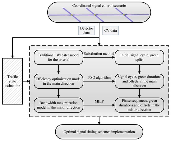
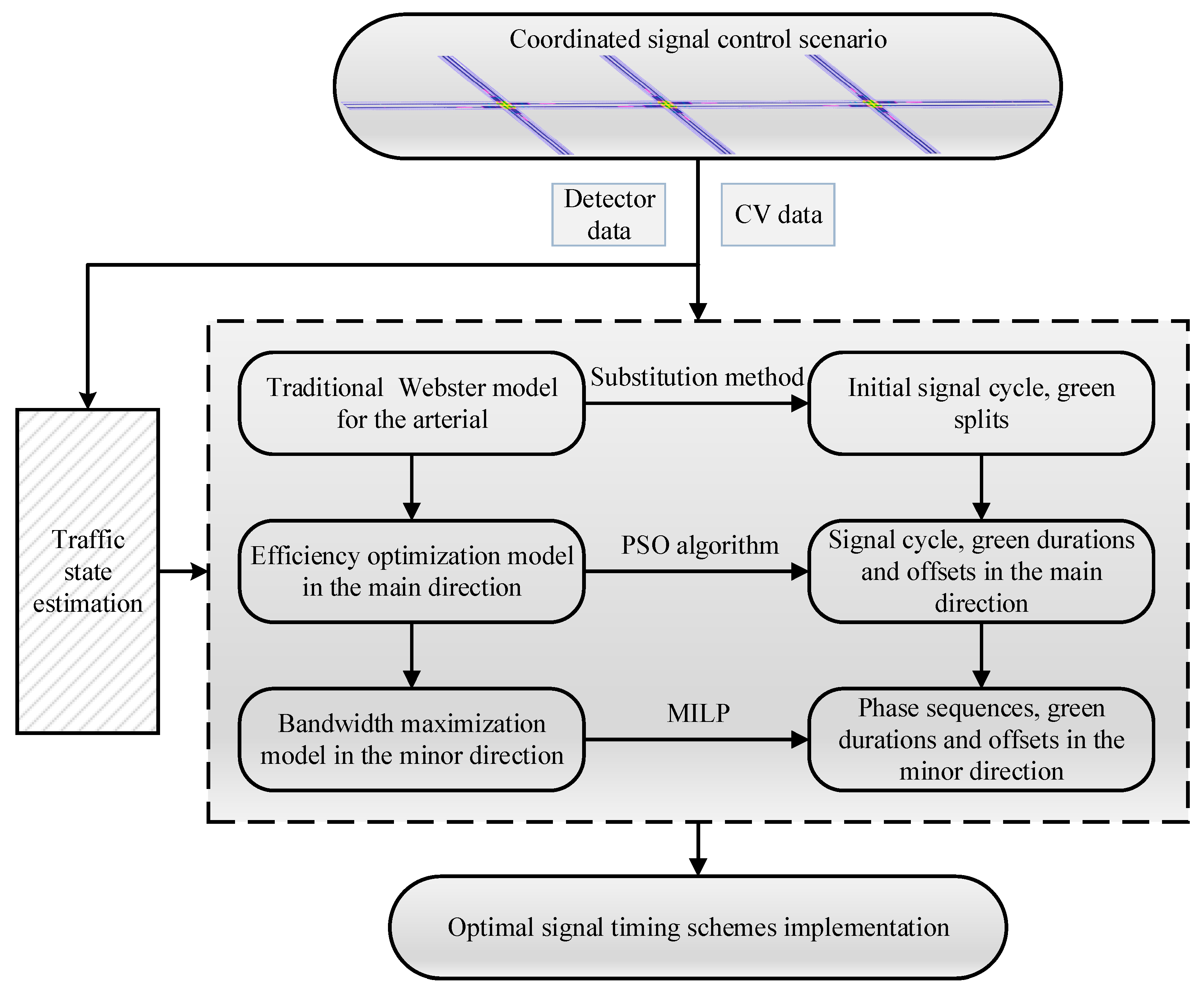
In this section, a hierarchical arterial signal coordinated control architecture model is developed for the asymmetric traffic, as shown in Figure 1. Considering the overall operation of arterial traffic, it is essential to reduce the negative impact of frequent changes in mainline signal timing on the operation of branch road traffic. To this end, within the signal control optimization, the phase sequence of branch roads remains unchanged. The execution sequence of phases is main road traffic, branch road through traffic, and branch road left turns. Additionally, the determination of green durations for branch roads is relatively independent from the optimization of mainline signal timing parameters.

Figure 1. Architecture diagram of the proposed approach.

In the mixed traffic environment, as driving behavior of CVs remains consistent with conventional vehicles, mixed traffic exhibits the same characteristics as conventional traffic flow. Accounting for the overall performance of the arterial traffic, the traditional Webster’s model is firstly utilized. It takes as the input the traffic flow data collected by fixed detectors at the entrance of each intersection, as in [35]. Based on the flow distribution among movements and different intersections, this model calculates the initial common signal cycle $C_0$ and the green splits for each intersection. The initial signal cycle serves as the basis for the following signal timing optimization, ensuring that the optimal signal cycle considers traffic conditions of each movement and intersection, and remains within a reasonable range. In addition, the initially determined green splits for branch road phases ensure that the green durations of branch road traffic are not significantly affected by the optimization of mainline traffic signal timings.

Then, based on the results of above calculation and traffic state estimation, the efficiency optimization model is developed for traffic flow in the main direction (the higher-volume direction) of the main road. This model takes as the control objective the weighted sum of the total travel time (TTT) and total travel distance (TTD), optimizing signal cycle, green durations and offsets in the main direction. In this process, the allowable range of signal cycle is limited based on the initial common signal cycle as its value meets the fundamental conditions in signal coordination control.

In the next step, the bandwidth maximization model in the minor direction of the main road takes the maximization of green wave bandwidth as the control objective. It determines the optimal mainline phase sequences, green durations and offsets in this direction. More detailed content regarding the method architecture is explained in the following text.

3.1. Traffic State Estimation Algorithm

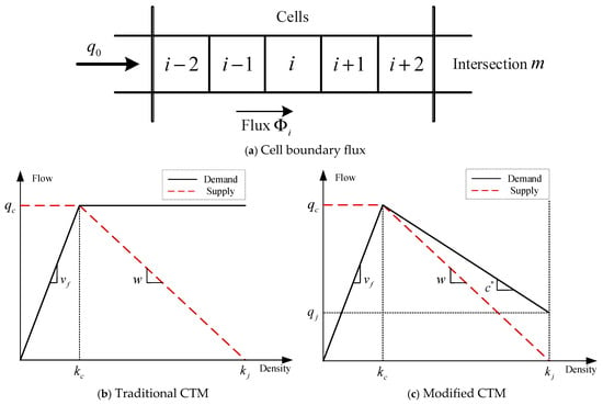
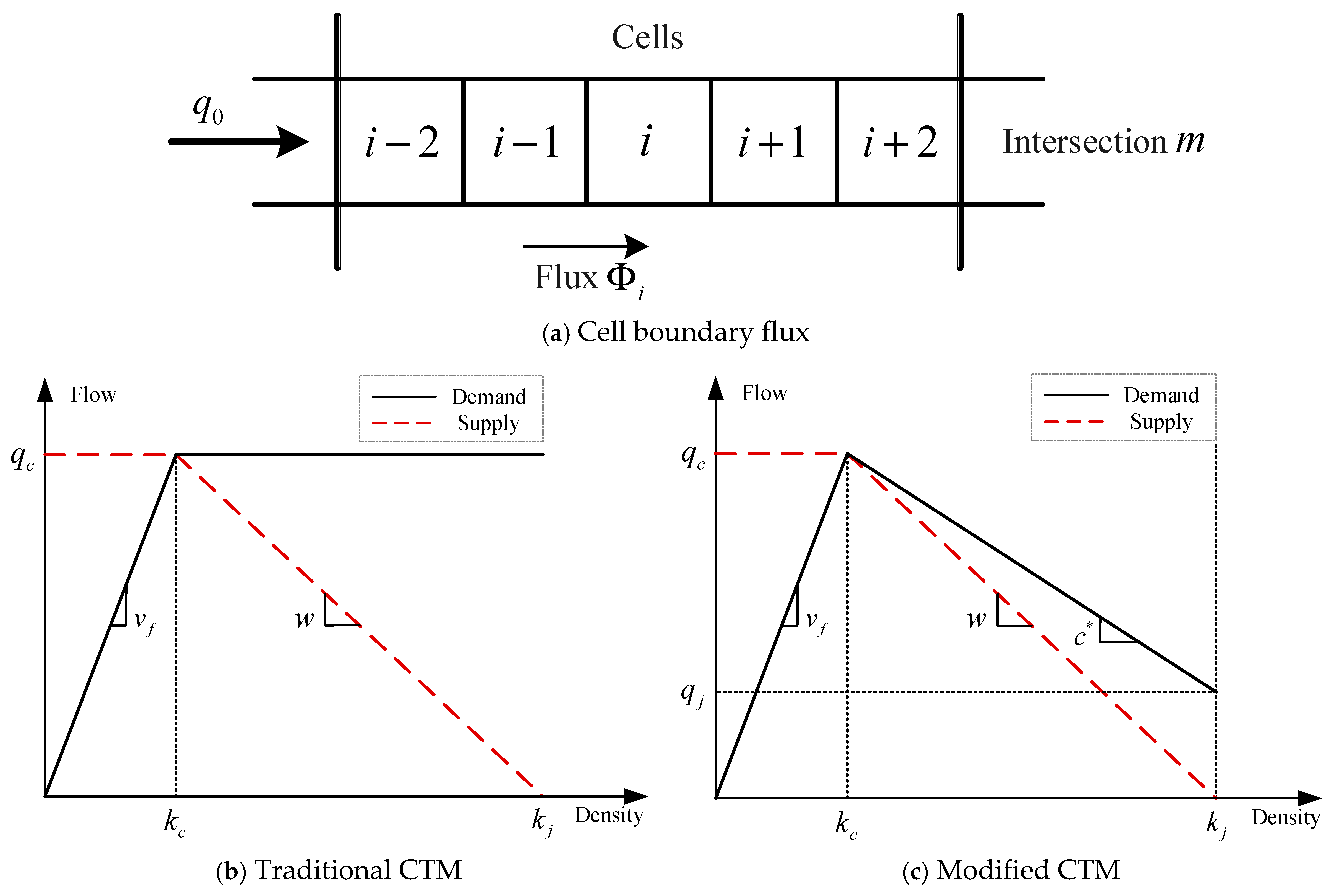
Some studies predict vehicle trajectories and calculate traffic delay value based on the predictions. However, this is not real-time due to the time-consuming computation. Thus, to represent traffic dynamics in the main direction of arterials, this study adopts the mCTM proposed by Srivastava et al. [36]. As illustrated in Figure 2a, the section upstream of intersection $m$ is divided into several consecutive cells. Meanwhile, the prediction period $t_p$ is also discretized into uniform intervals with a duration of $\Delta t$. For the time interval $k$, time period is represented as $\left(kT,\left(k+1\right)T\right]$, where $k=0,1,2,\mathrm{\dots },N_p$ and $N_p$ is number of intervals within the prediction horizon.

Figure 2. The illustrations of CTM and mCTM.

For a certain cell $i$, the cell length $\Delta x_i$ and time interval $\Delta t$ meet the Courant Friedrich Lewy condition [37], $\Delta x_i/\Delta t>v_f$, where $v_f$ is free flow speed. Within time interval $k$, the cell boundary flux from cell $i-1$ to cell $i$ is formulated as

$${\mathrm{\Phi }}_i\left(k\right)=\min \left\{D_{i-1}\left(k\right),S_i\left(k\right)\right\}$$

(1)

where $D_i$ and $S_i$ are the demand and supply function for cell $i$, respectively.

Corresponding to cell density ${\rho }_i$, changes in demand and supply values are shown in Figure 2b,c. Compared to the traditional CTM, the mCTM refines the definition of traffic demand in congested states, by adding the parameter of jam demand $q_j$. In the queue dispersion process of congested traffic, the traffic flow rate increases gradually to the capacity flow rate $q_c$ instead of maintaining a fixed value $q_c$. This agrees with the realistic queue discharge features at signalized intersections. The modified traffic demand is expressed as

$$D_i^{\prime }\left(k\right)=\min \left\{v_f{\rho }_i\left(k\right),q_j+c^{*}\left({\rho }_j-{\rho }_i\left(k\right)\right)\right\}$$

(2)

where ${\rho }_j$ is jam density, and $c^{*}$ is the slope of demand function in congested states.

Additionally, traffic supply in the mCTM stays the same as the CTM, shown as

$$S_i\left(k\right)=\min \left\{q_c,w\left({\rho }_j-{\rho }_i\left(k\right)\right)\right\}$$

(3)

where $w$ is the slope of supply function in congested states. The updated boundary flux and cell density are formulated as

$${\mathrm{\Phi }}_i\left(k\right)=\min \left\{D_{i-1}^{\prime }\left(k\right),S_i\left(k\right)\right\}$$

(4)

$${\rho }_i\left(k+1\right)={\rho }_i\left(k\right)+{\displaystyle \frac{\Delta t}{\Delta x_i}}\left({\mathrm{\Phi }}_i\left(k\right)-{\mathrm{\Phi }}_{i+1}\left(k\right)\right)$$

(5)

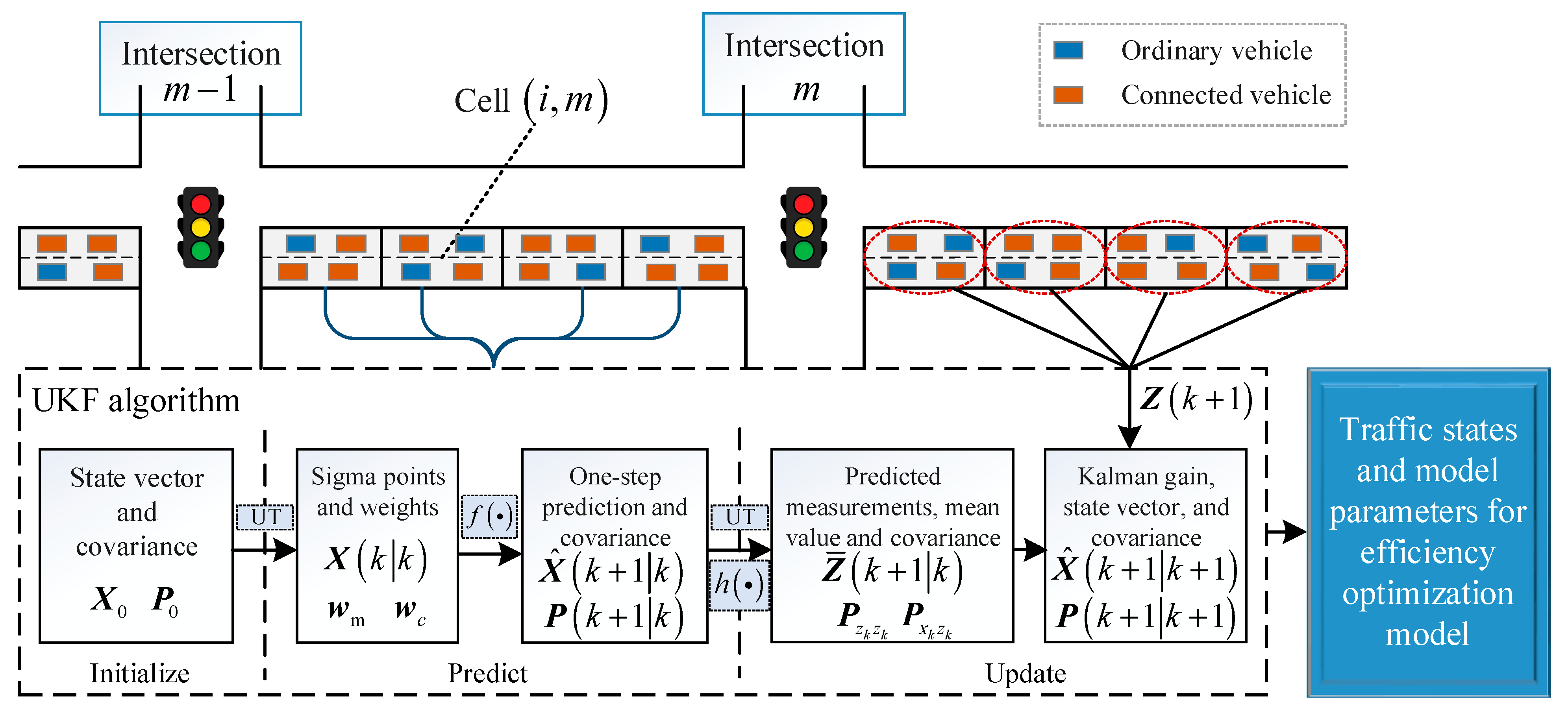
Before the implementation of the signal coordinated control approach, the original values of cell states and model parameters of mCTM are assumed to be known. Within each control iteration with the duration of $t_c$, to align the prediction results of mCTM with time-varying traffic flow characteristics, the Unscented Kalman Filter (UKF) algorithm is used to calibrate cell states and model parameter values at the beginning of the control process. The UKF algorithm is a nonlinear filtering method proposed by Julier and Uhlmann [38], adopted here as it is comparatively more accurate and more stable than the Extended Kalman Filter [39,40].

As illustrated in Figure 3, the traffic state estimation algorithm based on the UKF mainly involves three stages: initialization, prediction, and update. In the initialization stage, the state vector ${\mathit{X}}_0$ and its variance ${\mathit{P}}_0$ are set. ${\mathit{X}}_0$ includes cell states and model parameters, whose values are determined according to the original assumptions or the estimation results of the latest iteration.

Figure 3. Schematic diagram of traffic state estimation algorithm.

Then, in the prediction stage, through Unscented Transform (UT), Sigma points $\mathit{X}\left(k\left|k\right.\right)$ and corresponding weights ${\mathit{w}}_{\mathrm{m}}$ and ${\mathit{w}}_c$ are generated. The one-step prediction of Sigma points and the covariance, $\widehat{\mathit{X}}\left(k+1\left|k\right.\right)$ and $\mathit{P}\left(k+1\left|k\right.\right)$ are obtained through the nonlinear state equation $f\left(·\right)$. This actually corresponds to the iterative computation process of mCTM.

Finally, in the update stage, another UT is conducted for a new Sigma point set of $\widehat{\mathit{X}}\left(k+1\left|k\right.\right)$. The Sigma points are then used through the observation function $h\left(·\right)$ to obtain the prediction measurements $\overline{\mathit{Z}}\left(k+1\left|k\right.\right)$, the mean value ${\mathit{P}}_{z_k{z}_k}$ and covariance ${\mathit{P}}_{x_k{z}_k}$. This observation function corresponds to the determination process of cell speeds, referring to the fundamental diagram in Figure 2. Meanwhile, the actual observed cell speeds $\mathit{Z}\left(k+1\right)$ are achieved by averaging the CV velocities detected within the certain cell. Based on the above, the Kalman gain, state vector $\widehat{\mathit{X}}\left(k+1\left|k+1\right.\right)$ and covariance $\mathit{P}\left(k+1\left|k+1\right.\right)$ are updated for the following efficiency optimization model and the next iteration of the estimation process.

More detailed descriptions of the UKF algorithm could be found in [38], which are simplified here due to limited space.

3.2. Efficiency Optimization Model

Based on the initial signal cycle and green splits, the efficiency optimization model aims to optimize common signal cycle, green durations of through traffic and offsets in the main direction, ensuring smooth transportation operation.

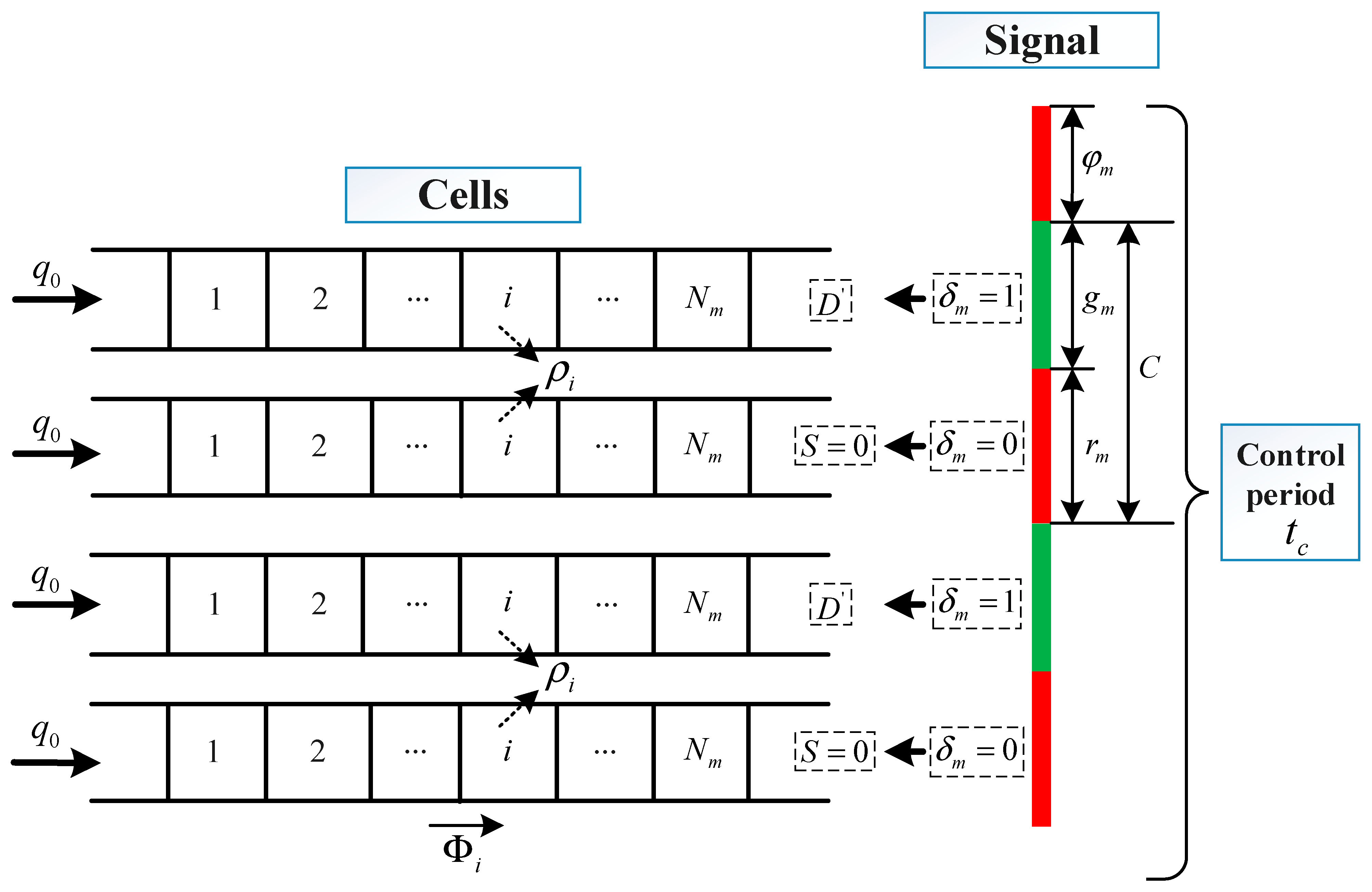
In this direction, the signal control for intersection $m$ is illustrated in Figure 4. The signal state distribution is jointly regulated by signal cycle $C$, green duration $g_m$ and offset ${\phi }_m$. The signal display state is represented by ${\delta }_m$, being “1” for green and “0” for red. When ${\delta }_m$ changes from 1 to 0, i.e., when the red light is activated, the intersection permits no longer vehicle inflow. Referring to Equation (3), traffic supply downstream of cell $N_m$ equals to 0. When ${\delta }_m$ changes from 0 to 1, i.e., when the green light is activated, queued vehicles upstream of the intersection are released. Referring to Equation (2), traffic demand of cell $N_m$ in current time interval $k$ is expressed as $D_i^{\prime }\left(k\right)=q_j+c^{*}\left({\rho }_j-{\rho }_{N_m}\left(k\right)\right)$.

Figure 4. Signal control schematic diagram of the main direction.

Thus, under varying traffic signal states, given the initial cell states and upstream and downstream flows, the density state of each cell within the control period $t_c$ is updated referring to Equation (5).

TTT and TTD, derived from density states, have been widely used as control objectives to reduce traffic density and increase traffic flow, respectively [41,42]. The weighted sum of TTT and TTD is taken as the performance indicator in the current optimization model, as formulated in Equation (6). The first term represents TTT, decreasing queue length and queue duration upstream of intersections. The second term represents TTD, raising the traffic volume through the arterial within the control period. $N_c$ denotes the number of time intervals in the control horizon $t_c$; $N_{\mathrm{in}}$ is the number of intersections involved in the control process; $N_m$ is the number of cells upstream of intersection $m$; ${\alpha }_{\mathrm{TTT},m}$ and ${\alpha }_{\mathrm{TTD},m}$ are weighting coefficients of TTT and TTD for intersection $m$, respectively. In Equation (6), ${\delta }_m$ is applied to represent the integrated value of TTT (during red) and TTD (during green).

Equations (7)–(9) constrain the range of values for $C$, $g_m$ and ${\phi }_m$, respectively. Based on the initial signal cycle $C_0$, the maximum variable range of $C$ is $\Delta c_{\max }$. The green duration of intersection $m$ is limited by the minimum $g_{\min }$ and maximum $g_{\max }$. ${\phi }_m$ is non-negative and less than $C$.

Optimization objective:

$$\min Y={\displaystyle \sum _{k=1}^{N_p}{\displaystyle \sum _{m=1}^{N_{\mathrm{in}}}\left[{\alpha }_{\mathrm{TTT},m}\left(1-{\delta }_m\right){\displaystyle \sum _{i=1}^{N_m}{\lambda }_{i,m}\Delta x_{i,m}{\rho }_{i,m}\left(k\right)-{\alpha }_{\mathrm{TTD},m}{\delta }_m{\displaystyle \sum _{i=1}^{N_m}{\lambda }_{i,m}\Delta x_{i,m}{\rho }_{i,m}\left(k\right)v_{i,m}\left(k\right)}}\right]}}$$

(6)

Subject to

$$C_0-\Delta c_{\max }\le C\le C_0+\Delta c_{\max }$$

(7)

$$g_{\min }\le g_m\le g_{\max }$$

(8)

$$0\le {\phi }_m\le C$$

(9)

3.3. Bandwidth Maximization Model

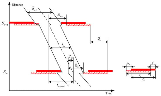
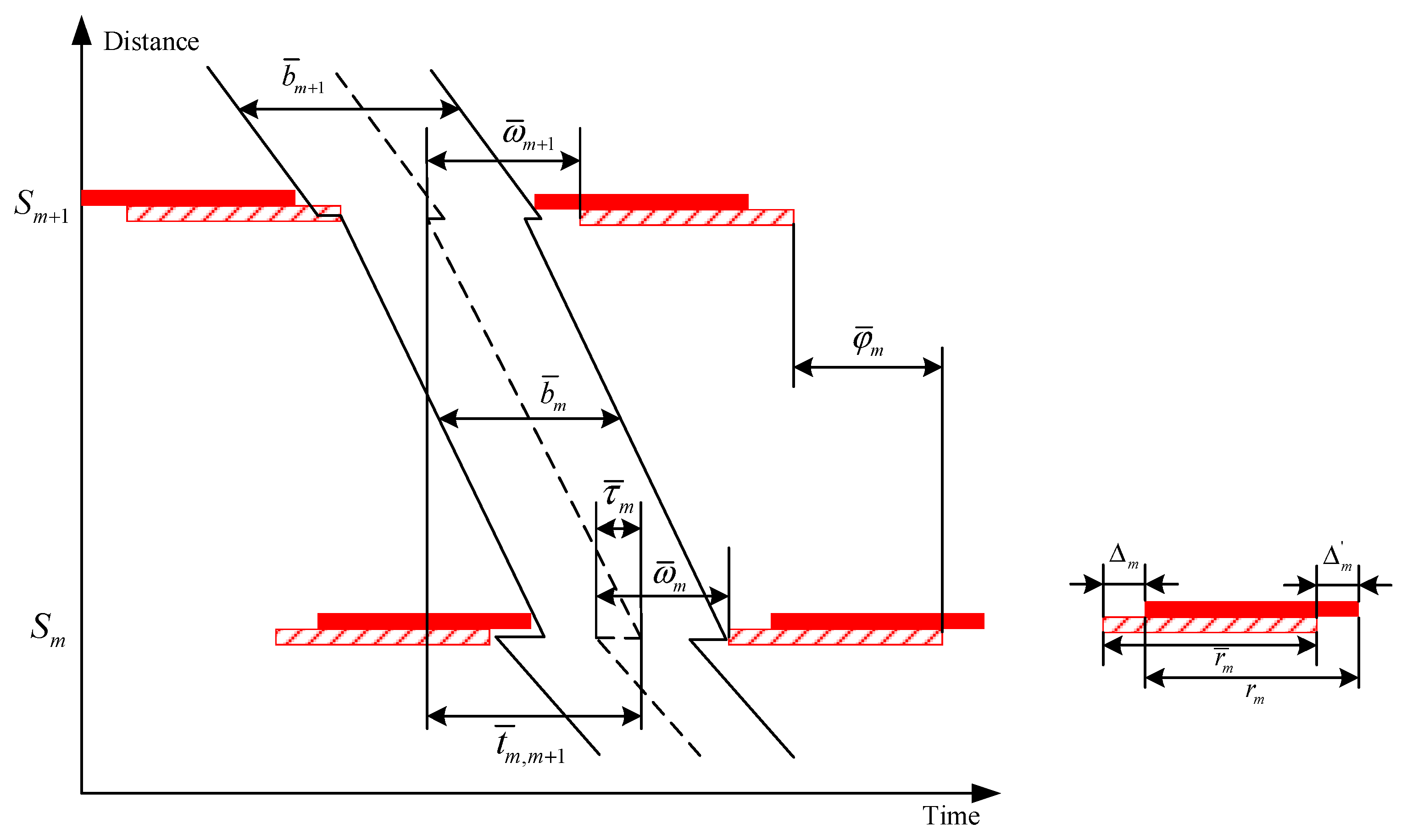
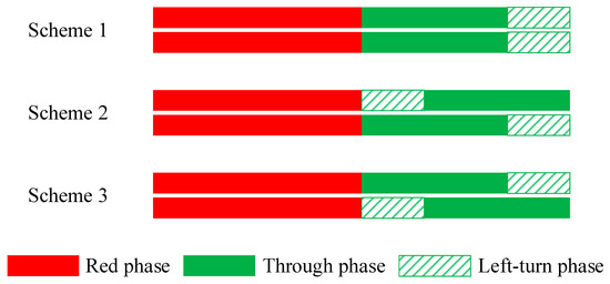
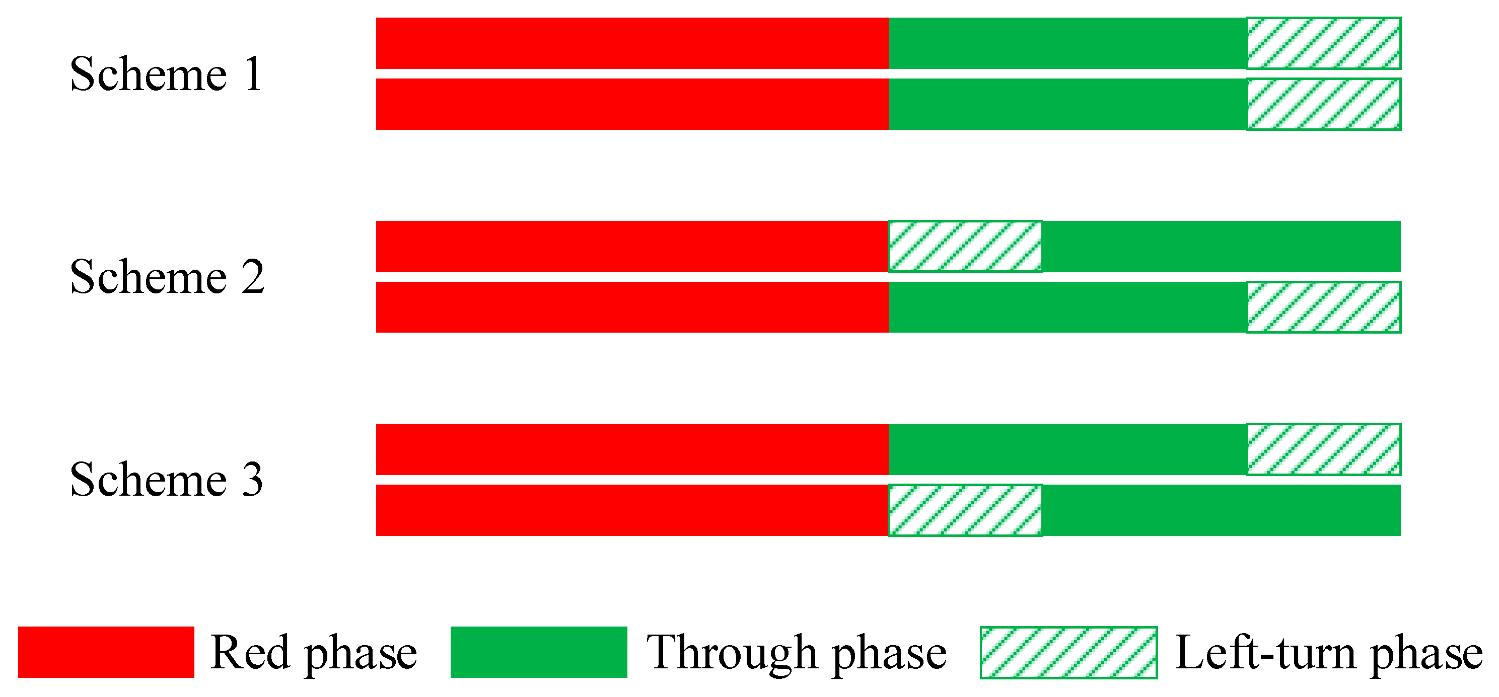
Based on the above calculation results, the bandwidth maximization model determines phase sequences and values of remaining signal timing parameters, green durations and offsets in the minor direction. Figure 5 illustrates the distribution of signal timings in this direction, and its relationship with signal timing parameters of the main direction. The three options for phase sequences of the mainline traffic are shown in Figure 6.

Figure 5. Green wave diagram in the minor direction.

Figure 6. Selections of phase sequence.

The bandwidth maximization problem seeks for the maximum of the sum of green wave bandwidths in the minor direction, as formulated in Equation (10). ${\overline{b}}_m$ denotes the green wave bandwidth between intersection $m+1$ and $m$. The value of each green wave bandwidth results from the combined effects of multiple other parameters, green durations ${\overline{g}}_m$ and $g_m$, offsets ${\phi }_m$ and ${\overline{\phi }}_m$, ${\overline{\omega }}_m$ denoting the time from the middle line of the green band to the left side of red, and ${\overline{\tau }}_m$ denoting the queue clearance time.

Equations (11)–(13) constrain the range of values for ${\overline{b}}_m$, ${\overline{\omega }}_m$ and ${\overline{\phi }}_m$, respectively. ${\overline{b}}_m$ is not less than the minimum ${\overline{b}}_{\min }$. ${\overline{\omega }}_m$ and ${\overline{\phi }}_m$ are non-negative, and ${\overline{\phi }}_m$ is less than $C$. Equations (14)–(19) represent the mathematical relationships among the signal timing parameters in Figure 5. ${\overline{U}}_m$ is an integer, commonly set to −1, 0 or 1. In Equation (20), green duration ${\overline{g}}_m$ is constrained by the minimum value $g_{\min }$, and the maximum value $g_{\max }$. Equations (21) and (22) respectively constrain parameters ${\Delta }_m$ and ${\Delta }_m^{\prime }$ to ensure an overlap in the green timings of both directions, preventing the bi-directional signal timing plans from deviating excessively. Corresponding to Scheme 2 and Scheme 3 in Figure 6, green durations for left turns are not less than $g_{\min }$, as shown in Equation (23).

Optimization objective:

$$\max Q={\displaystyle \sum _{m=1}^{N_{\mathrm{in}}-1}{\overline{b}}_m}$$

(10)

Subject to

$${\overline{b}}_m\ge {\overline{b}}_{\min }$$

(11)

$${\overline{\omega }}_m\ge 0$$

(12)

$$0\le {\overline{\phi }}_m\le C$$

(13)

$${\overline{\omega }}_m\ge {\displaystyle \frac{{\overline{b}}_m}{2}}+{\overline{\tau }}_m$$

(14)

$${\overline{\omega }}_{m+1}\ge {\displaystyle \frac{{\overline{b}}_m}{2}}$$

(15)

$${\overline{\omega }}_m+{\displaystyle \frac{{\overline{b}}_m}{2}}-{\overline{\tau }}_m\le C-{\overline{r}}_m$$

(16)

$${\overline{\omega }}_{m+1}+{\displaystyle \frac{{\overline{b}}_m}{2}}\le C-{\overline{r}}_{m+1}$$

(17)

$${\overline{\phi }}_m+{\phi }_{m+1}+{\Delta }_{m+1}-{\Delta }_m-{\overline{U}}_{m}C=0$$

(18)

$${\overline{\phi }}_m+{\overline{r}}_{m+1}+{\overline{\omega }}_{m+1}-{\overline{t}}_{m,m+1}-{\overline{r}}_m-{\overline{\omega }}_m+{\overline{\tau }}_m=0$$

(19)

$$g_{\min }\le {\overline{g}}_m\le g_{\max }$$

(20)

$$-g_m\le {\Delta }_m\le {\overline{g}}_m$$

(21)

$$-{\overline{g}}_m\le {\Delta }_m^{\prime }\le g_m$$

(22)

$$\left|{\Delta }_m\right|\ge g_{\min } \mathrm{and} \left|{\Delta }_m^{\prime }\right|\ge g_{\min }, if {\Delta }_m\ne 0$$

(23)

3.4. Model Solution Algorithm

In the hierarchical arterial signal coordinated control approach, as illustrated in Figure 1, three different methods are in turn utilized to solve the models for the arterial, the main direction and the minor direction of the main line. Firstly, to ensure proper traffic operation of the arterial including both main road and branch roads, the initial signal cycle and green split of each phase are calculated. And then, traffic efficiency in the main direction with a higher traffic volume is taken into account. The common signal cycle, green durations and offsets in this direction are optimized. Lastly, for light traffic flow in the minor direction, the sum of green wave bandwidths is maximized, to optimize mainline phase sequences, green durations and offsets in the current direction. The specific steps for solving this signal coordinated control problem are as follows.

Step 1: Solve the traditional Webster’s model for the arterial. As a rational function with both numerator and denominator being linear functions, the cycle formula in this model can be easily solved through the substitution method. On the basis of the traffic flow data, the initial signal cycle and green splits are obtained.

Step 2: Solve the efficiency optimization model in the main direction. The efficiency optimization model is a complex nonlinear model, as its control objective is the integration of cell states within the control time horizon. This model is solved by the PSO algorithm (referring to [28,43]), optimizing the common signal cycle, green durations and offsets in the main direction.

Step 3: Solve the bandwidth maximization model in the minor direction. As both the control objective and constraints can be expressed linearly, the maximization problem for green wave bandwidths is formulated as a MILP model. It is solved by the linprog function in the field of computing, obtaining phase sequences, green durations and offsets in the minor direction.

The computational operations of Steps 1 and 3 are extremely simple, and the real-time performance of the coordinated signal control mainly depends on the computation time of Step 2.

4. Case Study

4.1. Study Site

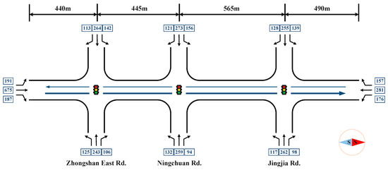
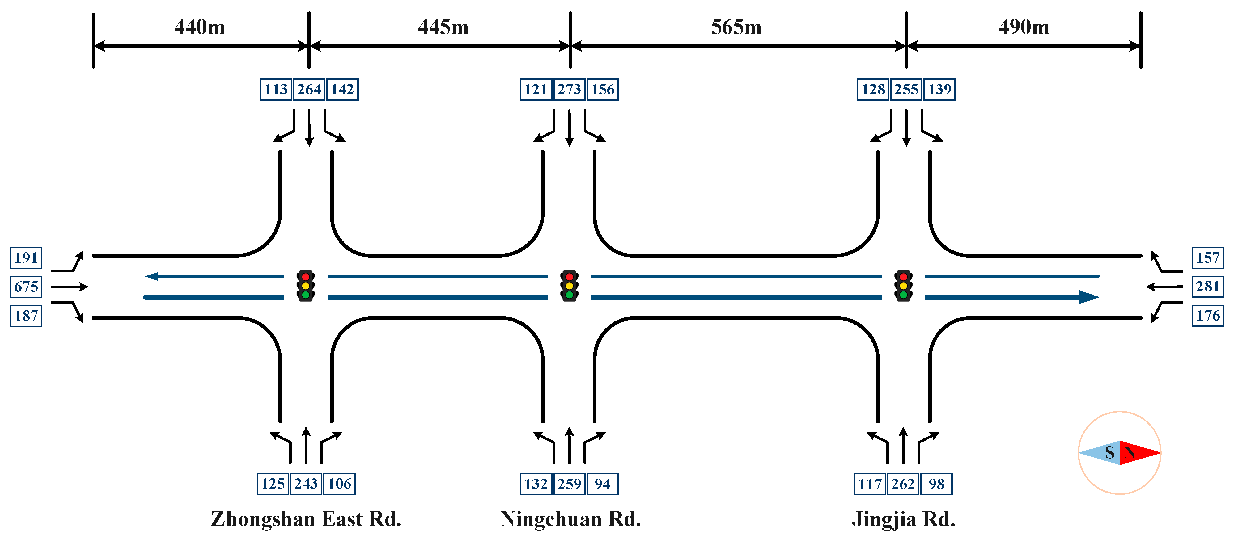
The effectiveness of the proposed approach is assessed in the simulation environment built by VISSIM software. The simulated road structure is based on a section of Shiji Avenue, Ningbo City, Zhejiang Province. There are three consecutive intersections involved, as demonstrated in Figure 7, from Zhongshan East Road to Jingjia Road. The distribution status among intersections and the traffic demand flow rate (veh/h/lane) of each entrance have also been illustrated. Traffic detectors are located at the stop lines of each intersection, to measure passing traffic volumes. In the simulation run, traditional detector data is aggregated every 60 s, and CV data is collected at the moment of control activation. Both of them are obtained through the COM interface and transmitted to the coordinated signal control model developed in MATLAB. After the values of optimal signal timing parameters calculated, the updated signal timing scheme is transmitted back to the simulation environment, and corresponding signal control instructions are executed.

Figure 7. Coordinated signal control site.

For each simulation run, the simulation period is set to be 3600 s, with the initial 5 min being the warm-up time. The simulation resolution is 6 time steps/simulation second. To simulate scenarios under various penetration rates of CVs, the proportion of CVs in the vehicle composition setting varies from 10% to 90% in increments of 20%. As inflow from each entrance is based on the same composition, the distribution of CVs in the mixed traffic are generally consistent with the predefined values.

For the coordinated signal control approach, the parameter setting is shown in Table 2. The first four parameters belong to mCTM, and the original values are obtained through calibration before the simulation run. The following three vectors belong to the UKF algorithm, including the initial state covariance matrix $P_0$, process noise covariance matrix $Q$ and measurement noise covariance matrix $R$. The first element of each vector denotes the cell density and the remaining elements correspond one-to-one to the elements of the mCTM mentioned above. The length of cells along the arterial $\Delta x$, ranges from 39 to 50 m, depending on the structural characteristics of the location.

Table 2. Parameter setting of the coordinated signal control approach.

Parameter	Setting Value	Unit
$v_f$	55	km/h
${\rho }_j$	116.1	veh/km
${\rho }_c$	36.9	veh/km
$q_j$	550	veh/h
$P_0$	[90, 5.6, 30, 15, 2250]	-
$Q$	[30, 3, 10, 5, 500]	-
$R$	25	-
$\Delta x$	39~50	m
$\Delta t$	2.5	s
$t_c$	8	min
$\Delta c_{\max }$	15	s
${\overline{b}}_{\min }$	15	s
$g_{\min }$	15	s
$g_{\max }$	65	s
${\alpha }_{\mathrm{TTT},1}$, ${\alpha }_{\mathrm{TTT},2}$, ${\alpha }_{\mathrm{TTT},3}$	0.5, 1.5, 1.0	-
${\alpha }_{\mathrm{TTD},1}$, ${\alpha }_{\mathrm{TTD},2}$, ${\alpha }_{\mathrm{TTD},3}$	0.015, 0.03, 0.025	-

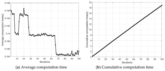
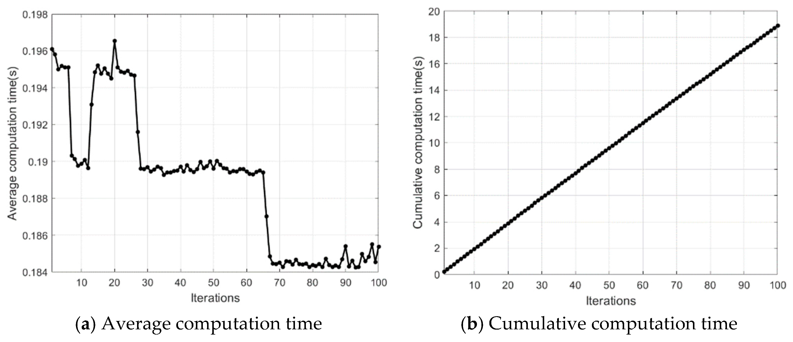
In the solution process, the PSO algorithm is configured with the following parameters. The swarm size is set to 50 particles. The maximum number of iterations is 100. Both acceleration coefficients are fixed 2.0, and the inertia weight is updated as $\mu =\mu *0.99$ with an initial value of 1. The maximum velocity is constrained to 10% of the decision variable bounds. The algorithm terminates when either the maximum number of iterations is reached or the global best fitness value does not improve by more than 1 × 10⁻⁴ over 10 consecutive generations. This algorithm was conducted on a laptop equipped with an Intel Core i7-13700K processor and 16 GB of RAM. The average and cumulative computation time of iterations are respectively illustrated in Figure 8. Most iteration processes converge within 50 generations, less than 10 s. This time can be significantly decreased with a higher-performance computer. During the transition period between old and new signal timing schemes, the computation can be completed simultaneously, for real-time implementation.

Figure 8. Computation time of iterations.

As for the MILP problem of the minor direction, it is solved by the intlinprog solver in MATLAB, configured with a Constraint Tolerance of 1 × 10⁻⁶, an Integer Tolerance of 1 × 10⁻⁶, and a Relative Gap Tolerance of 1 × 10⁻³.

The values of weighting coefficients ${\alpha }_{\mathrm{TTT},m}$, ${\alpha }_{\mathrm{TTD},m}$ are determined by comparing performance indicators under multiple combinations.

For comparison, the performance of the proposed coordinated signal control model is compared to the Synchro model and the MULTIBAND model. The network structure, traffic volumes and traffic rules, and parameter range in their simulation scenarios are identical to those of the proposed model. In version 7 of the Synchro software, the optimal signal timing scheme is obtained through the embedded optimization model. The optimization problem of MULTIBAND is presented as an MILP model, which executes the bandwidth maximization for both the main and minor directions. It is also solved by the intlinprog solver in version 2018 of the MATLAB software, with same parameter values as those in the proposed model. Simulation evaluation results include performance indicators for the arterial, the main road, and the two different directions of the main line.

4.2. Result Analysis

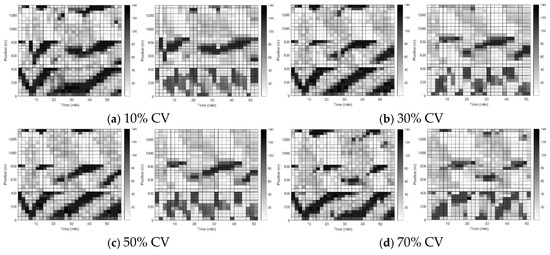
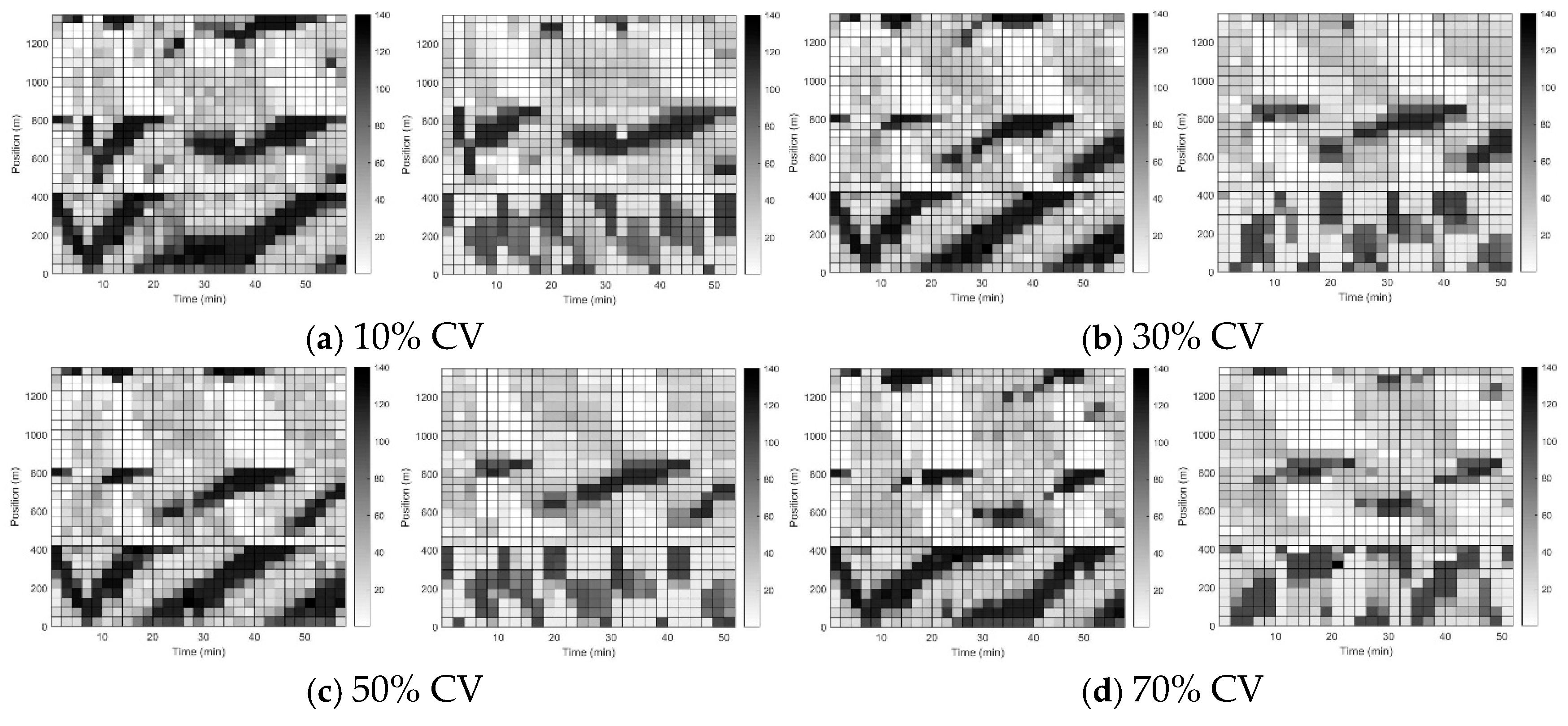
The effectiveness of the traffic state estimation algorithm is first tested. To increase the randomness, different signal control schemes are respectively implemented in scenarios with various CV penetration rates. As demonstrated in Figure 9, the horizontal axis represents density values are collected every 2 min. The vertical axis represents the cell locations. The first intersection is located at around 400 m, the second at around 800 m, and the third at around 1300 m. The internal space of the intersections is not considered. The color of each cell represents the current density value, with the unit being veh/h.

Figure 9. Distribution of cell density with various CV penetration rates.

For each case, left side shows the real distribution, and the right side shows the evaluation results. It can be shown that with the increase in CV penetration rates, the estimation accuracy of traffic characteristics is improved, especially for traffic congestions. Moreover, when the penetration rate exceeds 50%, the distribution of low cell density can also be captured more accurately.

The performance indicators under three different signal control models are illustrated in Table 3, for the arterial, main road, main direction (northbound) and minor direction (southbound) of the mainline. Their values are the averages of three runs with different random seeds, with standard deviations in parentheses. Among them, AD denotes the average delay, QL denotes the average queue length, NS denotes the number of stops, and ATT denotes the average travel time. For the proposed coordinated signal control model, two scenarios with 10% and 30% CVs are discussed to assess its effectiveness in low penetration rates.

Table 3. Performance of various models.

	Indicator	Synchro	MULTIBAND	Coordinated (10% CV)	Coordinated (30% CV)
Arterial	AD (s)	180.8(8.90)	126.7(8.67)	127.8(9.73)	111.8(6.19)
	QL (veh)	140.3(6.14)	89.3(7.64)	71.9(4.31)	64.8(5.67)
	NS	4.4(0.32)	3.1(0.25)	2.2(0.08)	2.0(0.11)
Mainline	ATT (s)	258.7(1.7)	284.0(1.41)	304.7(8.62)	292.0(8.89)
	AD (s)	136.3(1.25)	162.0(1.41)	183.3(9.07)	169.7(8.33)
	NS	3.0(0)	3.0(0)	4.0(0)	3.3(0.58)
Northbound (main)	ATT (s)	284.1(3.23)	322.3(3.05)	327.9(13.86)	313.2(3.2)
	AD (s)	162.0(2.98)	200.3(3.02)	206.4(13.91)	191.6(3.12)
	NS	3.1(0.06)	4.2(0.15)	4.2(0.13)	3.8(0.23)
Southbound (minor)	ATT (s)	191.7(5.69)	194.8(10.23)	250.2(5.65)	243.8(36.05)
	AD (s)	69.9(6.03)	72.9(10.09)	128.0(5.3)	121.6(36.22)
	NS	1.9(0.17)	1.9(0.31)	2.9(0.04)	2.5(0.78)

By comparing the MULTIBAND model and the Synchro model, it can be found that the MULTIBAND model underperforms the Synchro model in mainline traffic operation, especially the main direction traffic with much higher ATT, AD and NS. However, the former significantly performs better than the latter in indicators of arterial traffic. This indicates that the Synchro model focuses on the mainline traffic operation at the expense of branch roads. On the other hand, although the MULTIBAND model lacks adaptation to the arterial asymmetric traffic, it still maintains the overall operational performance.

When the coordinated model is compared to the MULTIBAND model, it performs worse in almost all indicators with 10% CV penetration. This mainly results from the poor performance of traffic estimation and prediction. Consequently, the optimal signal timing scheme deviates from the actual traffic conditions. As the penetration rate increases to 30%, indicators of arterial traffic and mainline traffic are obviously improved. With the more accurate prediction of traffic characteristics, mainline signal timings are closer to current needs.

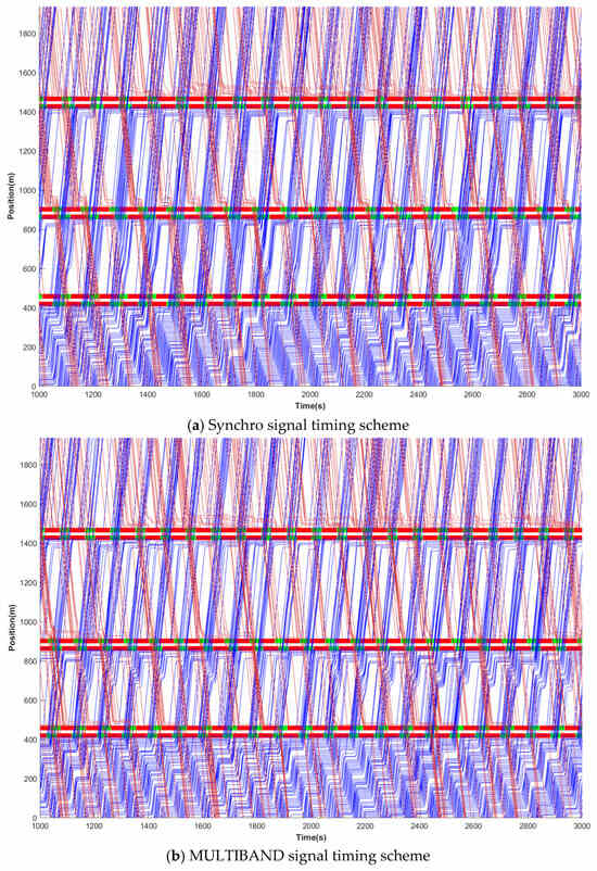
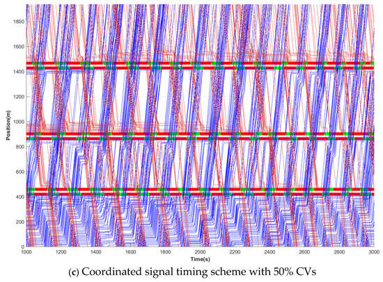
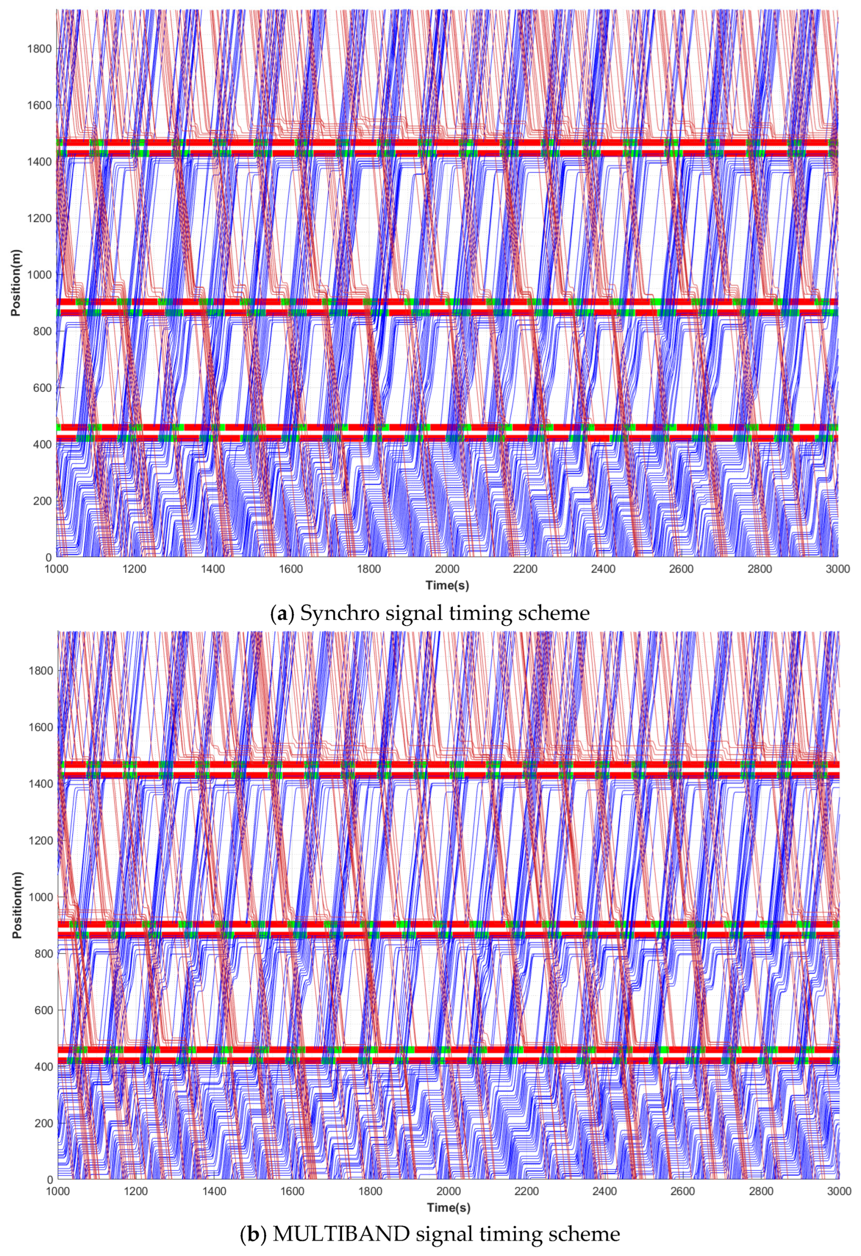
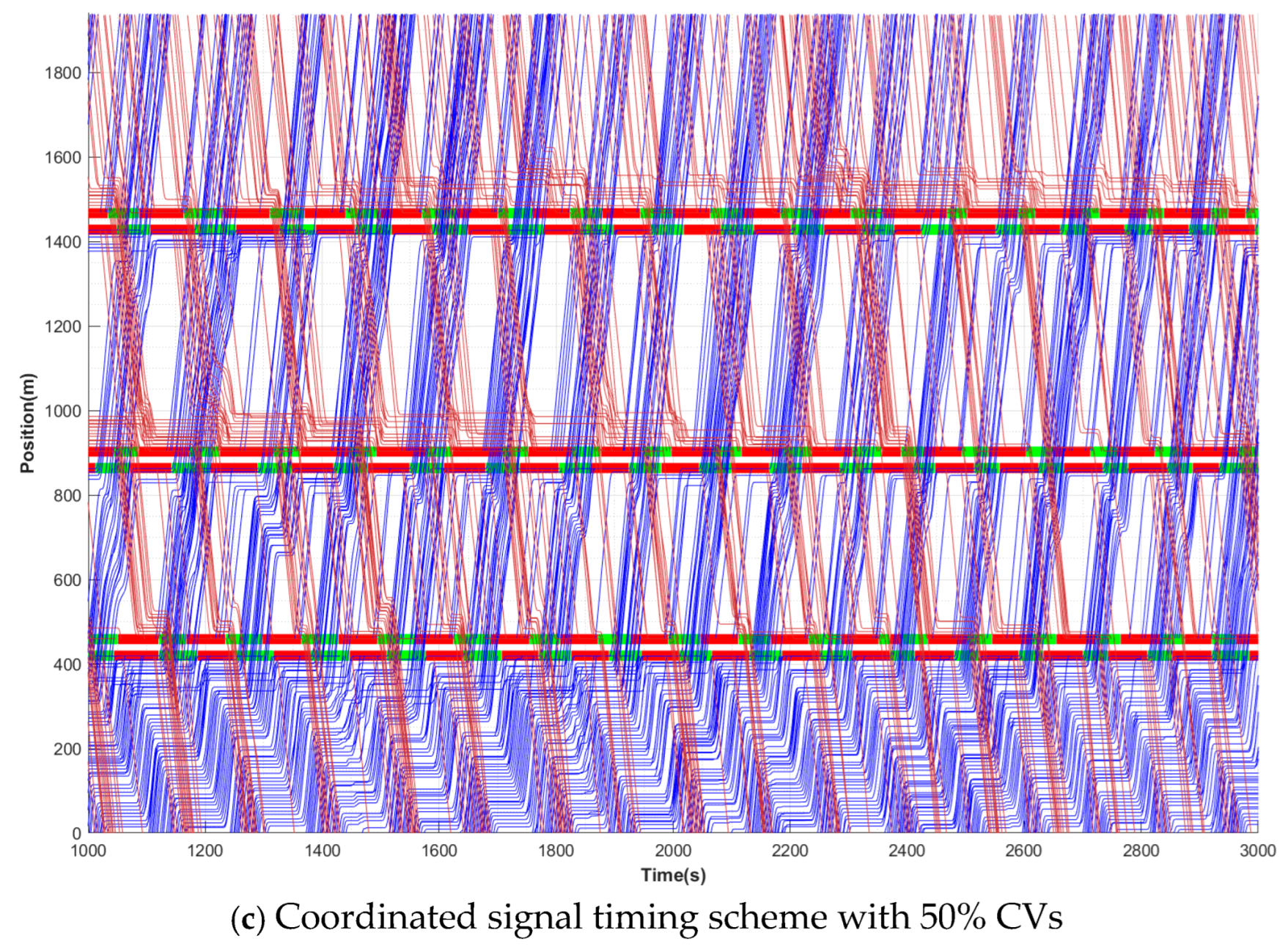
In addition to the numerical performance measures in Table 3, the spatiotemporal distribution of vehicle trajectories on the main road is demonstrated in Figure 10, for various control models. The blue line and the brick red line represent the trajectories in main direction and minor direction, respectively. To improve clarity, the number of displayed trajectory vehicles is halved. The horizontal axis represents the collection time of vehicle trajectory data, ranging from 1000 s to 3000 s. The vertical axis represents the position along the northbound road, starting at the most upstream point and ending at the most downstream point. The queuing status changes at each intersection are visually presented, which reflect the level of traffic flow smoothness on the arterial.

Figure 10. Trajectory diagrams of the arterial with various control models.

It is clear that queuing is infrequent under the Synchro model (Figure 10a), meaning that mainline traffic can pass through smoothly. As for the MULTIBAND model in Figure 10b, frequent queuing occurs in the main direction, especially at the second intersection. This situation corresponds to the indicators in the above table. In Figure 10c, main direction traffic flow is smooth under the coordinated model (50% CV penetration), with only occasional queuing occurring. A relatively high penetration rate of CVs can significantly enhance traffic operational efficiency in the main direction. Comparatively, the smoothness of the minor direction traffic is slightly less than the Synchro model and the MULTIBAND model. The efficiency improvement in the main direction has somewhat affected the minor direction.

Traffic throughputs of various control models in Table 4 corresponds to the above distribution under a complete simulation process of 3600 s. More vehicles pass through in the main direction under the Synchro model (1987 veh) than the MULTIBAND model (1930 veh). In contrast, the condition is inverted for minor direction traffic, with 1476 veh and 1579 veh for the Synchro model and the MULTIBAND model, respectively. Traffic throughputs in both directions under the coordinated model exceed those of the other two models, indicating that more vehicles can pass smoothly through the arterial.

Table 4. Traffic throughputs of various control models.

Control Models	Synchro	MULTIBAND	Coordinated
Northbound (veh)	1987	1930	2034
Southbound (veh)	1476	1549	1639

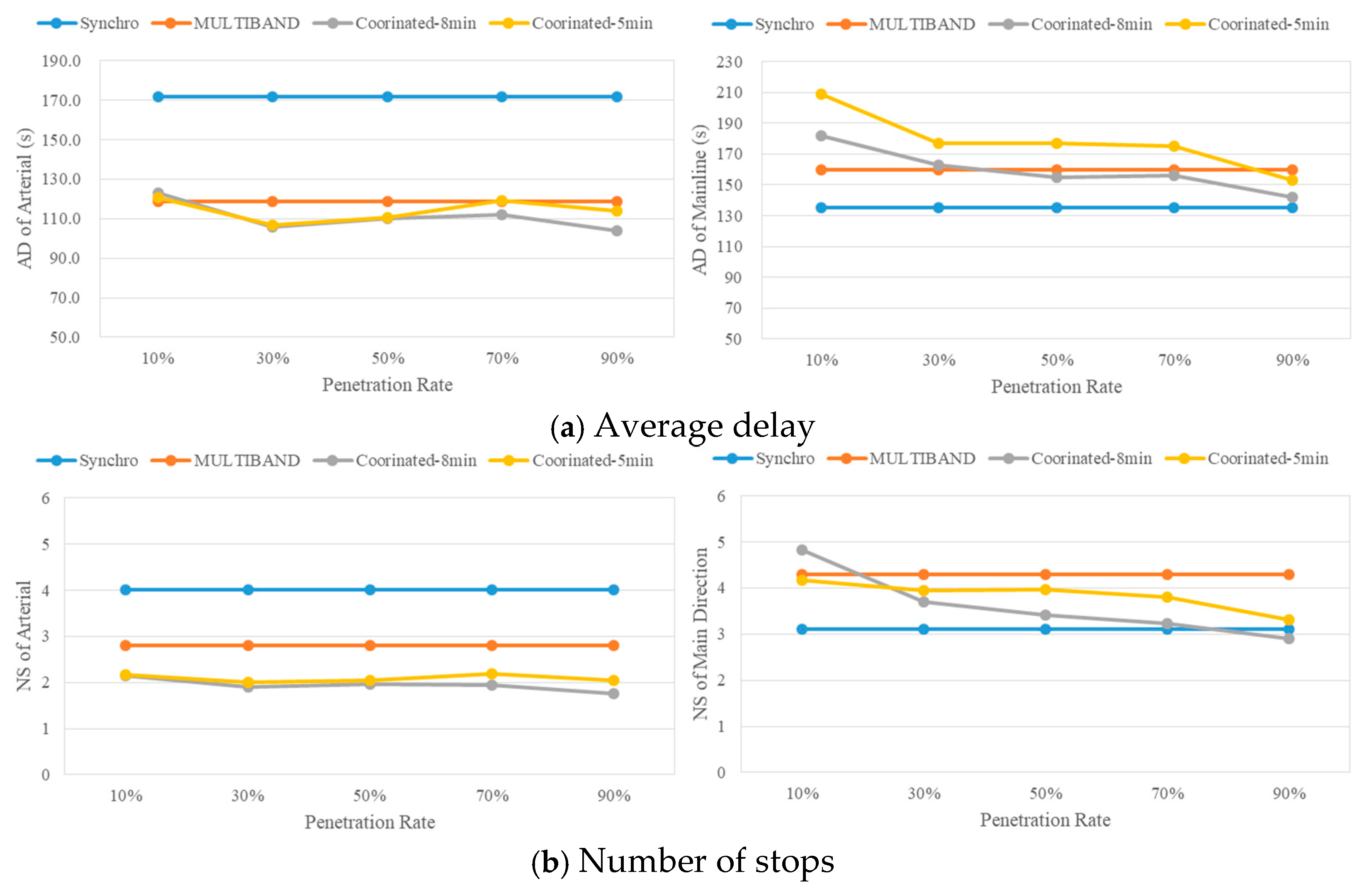
To analyze the impact of penetration rate of CVs, the performance indicators of the proposed coordinated control model are shown in Figure 11. In Figure 11a, the left side compares the average delay of arterial traffic. As the penetration rate rises from 10% to 30%, the indicator under the coordinated model declines to a point below the MULTIBAND model’s. Following this, the value fluctuates slightly with the increasing penetration rate, but remains consistently below the other two models.

Figure 11. Performance metric with various penetration rates of CVs.

The right side in Figure 11a illustrates the average delay of mainline traffic, and the value of the coordinated model exhibits a declining trend. When the penetration rate increases from 10% to 30%, the indicator of the coordinated model decreased markedly. Within scenarios with 50% or more CVs, the indicators of this model are less than that of the MULTIBAND model. The Synchro model consistently performs best, due to its control properties of giving grant absolute priority to mainline traffic.

The number of stops is illustrated in Figure 11b. The left side shows the number of stops of arterial, with the values of the coordinated model consistently fall below the other two models, indicating arterial traffic maintains relatively stable operation. The right side demonstrates the number of stops of main direction traffic. The indicator of the coordinated model has a clear downward trend, as the penetration rate rises. It falls below the MULTIBAND model at 30% CV penetration and below the Synchro model at 90% CV penetration.

To further analyze the influence of control horizon duration on control performance, performance indicators with 5 min and 8 min control periods are also compared in Figure 11. As the penetration rate of CVs increases, it is obvious that the trends of various performance indicators are similar with 5 min and 8 min control period, including the AD of mainline and the NS of main direction. However, the results under the 5 min condition are worse than those under the 8 min condition, with both AD of mainline and NS of main direction generally higher than the latter. Moreover, with the increase in the penetration rate, AD of arterial and NS of arterial under 5 min condition show fluctuations. This is mainly because the new signal timing scheme fails to transform smoothly from the previous one within a short control period, indicating that the switching of coordinated control should be less frequent.

It could be concluded that the impact of the CV penetration rate on the arterial traffic is slight. In contrast, its effect on the mainline traffic is significant.

5. Conclusions

This paper puts forward an arterial-level coordinated signal control approach for asymmetric traffic using partial CV information. The operational performance of arterial traffic is firstly considered, based on the traditional Webster’s model. Regarding mainline traffic, the efficiency optimization model is then developed for the main direction traffic flow with a higher volume. At last, the bandwidth maximization model is presented for traffic in the minor direction. This coordinated control model is solved sequentially by the substitution method, the PSO algorithm and the linprog function. The experimental results based on simulation scenarios show that compared to the other control models, the proposed coordinated model performs well with the penetration rate of CVs higher than 30%. The main contributions of this study are listed as follows.

On the basis of detector data and partial CV data, traffic state estimation algorithm is developed for the calibration of cell states and mCTM parameters. This intends to provide accurate prediction of traffic characteristics for the arterials under various control measures.

The hierarchical coordinated signal control structure is constructed, sequentially considering arterial traffic operation, main direction traffic and minor direction traffic of the mainline. This divides the coordinated signal control into components with distinct emphases, enabling the adaptability to varying scenarios.

The effectiveness of the coordinated signal control approach has been verified within various simulation scenarios, especially considering traffic throughput and smoothness. Additionally, with various penetration rates of CVs, the impact on arterial traffic and mainline traffic is analyzed.

While demonstrating efficacy, the proposed approach is not without limitations. Future research should focus on the following aspects.

Currently, the real-world deployment of coordinated signal control schemes is infeasible, due to the lack of access to the traffic management system. The application effects of the coordinated signal control model need to be further tested in real-world road scenarios, in collaboration with the local traffic authorities. The application scope could be expanded to arterials with more intersections and road networks, to verify its stability and adaptability.

The uncompleted cycle of the previous signal timing scheme in this study is compensated by ensuring the minimum green duration for each phase, before the new scheme is executed. Thus, the impact of other transition forms could be further explored.

References

- Sims, A.G.; Dobinson, K.W. The Sydney coordinated adaptive traffic (SCAT) system philosophy and benefits. IEEE Trans. Veh. Technol. 2013, 29, 130–137. [Google Scholar] [CrossRef] [Scilit]
- Hunt, P.B.; Robertson, D.I.; Bretherton, R.D.; Royle, M.C. The SCOOT on-line traffic signal optimisation technique. Traffic Eng. Control 1982, 23, 190–192. [Google Scholar]
- Ma, Y.; Su, D.; Li, Y.; Tian, C.; Meng, W. Spatial perception of tagged cargo using fused RFID and CV data in intelligent storage. IEEE Internet Things J. 2022, 10, 1574–1587. [Google Scholar] [CrossRef] [Scilit]
- Jiang, Q.; Nian, D.; Guo, Y.; Ahmed, M.; Yang, G.; Ma, J. Evaluating connected vehicle-based weather responsive management strategies using weather-sensitive microscopic simulation. J. Intell. Transp. Syst. 2023, 27, 92–110. [Google Scholar] [CrossRef] [Scilit]
- Kwesiga, D.K.; Guin, A.; Hunter, M. Adaptive transit signal priority based on deep reinforcement learning and connected vehicles in a traffic microsimulation environment. In Proceedings of the 2024 Winter Simulation Conference (WSC), Orlando, FL, USA, 15–18 December 2024; IEEE: New York, NY, USA, 2024. [Google Scholar]
- Peng, J.; Shangguan, W.; Chai, L.; Chen, J.; Peng, C.; Cai, B. V2X-Enabled platoon control for aperiodic congestion mitigation via moving bottlenecks in mixed traffic environments. IEEE Trans. Veh. Technol. 2026, 1–13. [Google Scholar] [CrossRef] [Scilit]
- Tan, C.; Ding, Y.; Yang, K.; Zhu, H.; Tang, K. Connected vehicle data-driven robust optimization for traffic signal timing: Modeling traffic flow variability and errors. IEEE Trans. Intell. Transp. Syst. 2025, 26, 21635–21650. [Google Scholar] [CrossRef] [Scilit]
- Ye, B.L.; Wu, W.; Mao, W. A two-way arterial signal coordination method with queueing process considered. IEEE Trans. Intell. Transp. Syst. 2015, 16, 3440–3452. [Google Scholar] [CrossRef] [Scilit]
- Chen, C.; Che, X.; Huang, W.; Li, K. A two-way progression model for arterial signal coordination considering side-street turning traffic. Transp. B Transp. Dyn. 2019, 7, 1627–1650. [Google Scholar] [CrossRef] [Scilit]
- Little, J.D.C.; Kelson, M.D.; Gartner, N.H. MAXBAND: A Versatile Program for Setting Signals on Arteries and Triangular Networks; Transportation Research Board: Washington, DC, USA, 1981. [Google Scholar]
- Gartner, N.H.; Assman, S.F.; Lasaga, F.; Hou, D.L. A multi-band approach to arterial traffic signal optimization. Transp. Res. Part B Methodol. 1991, 25, 55–74. [Google Scholar] [CrossRef] [Scilit]
- Zhang, C.; Xie, Y.; Gartner, N.H.; Stamatiadis, C.; Arsava, T. AM-band: An asymmetrical multi-band model for arterial traffic signal coordination. Transp. Res. Part C Emerg. Technol. 2015, 58, 515–531. [Google Scholar] [CrossRef] [Scilit]
- Ma, W.; Zou, L.; An, K.; Gartner, N.H.; Wang, M. A partition-enabled multi-mode band approach to arterial traffic signal optimization. IEEE Trans. Intell. Transp. Syst. 2018, 20, 313–322. [Google Scholar] [CrossRef] [Scilit]
- Xu, L.; Xu, J.; Qu, X.; Jin, S. An origin-destination demands-based multipath-band approach to time-varying arterial coordination. IEEE Trans. Intell. Transp. Syst. 2022, 23, 17784–17800. [Google Scholar] [CrossRef] [Scilit]
- Husch, D.; Albeck, J. Synchro 6: Traffic Signal Software, User Guide; Trafficware Corporation: Albany, CA, USA, 2003. [Google Scholar]
- Yang, K.; Menendez, M.; Zheng, N. Heterogeneity aware urban traffic control in a connected vehicle environment: A joint framework for congestion pricing and perimeter control. Transp. Res. Part C Emerg. Technol. 2019, 105, 439–455. [Google Scholar] [CrossRef] [Scilit]
- Al Islam, S.M.A.B.; Hajbabaie, A.; Aziz, H.M.A. A real-time network-level traffic signal control methodology with partial connected vehicle information. Transp. Res. Part C Emerg. Technol. 2020, 121, 102830. [Google Scholar] [CrossRef] [Scilit]
- Li, J.; Peng, L.; Hou, K.; Tian, Y.; Ma, Y.; Xu, S.; Qiu, T.Z. Adaptive signal control and coordination for urban traffic control in a connected vehicle environment: A review. Digit. Transp. Saf. 2023, 2, 89–111. [Google Scholar] [CrossRef] [Scilit]
- Feng, Y.; Head, K.L.; Khoshmagham, S.; Zamanipour, M. A real-time adaptive signal control in a connected vehicle environment. Transp. Res. Part C Emerg. Technol. 2015, 55, 460–473. [Google Scholar] [CrossRef] [Scilit]
- Liang, X.J.; Guler, S.I.; Gayah, V.V. An equitable traffic signal control scheme at isolated signalized intersections using connected vehicle technology. Transp. Res. Part C Emerg. Technol. 2020, 110, 81–97. [Google Scholar] [CrossRef] [Scilit]
- Liang, X.J.; Guler, S.I.; Gayah, V.V. A heuristic method to optimize generic signal phasing and timing plans at signalized intersections using connected vehicle technology. Transp. Res. Part C Emerg. Technol. 2020, 111, 156–170. [Google Scholar] [CrossRef] [Scilit]
- Ma, C.; Yu, C.; Zhang, C.; Yang, X. Signal timing at an isolated intersection under mixed traffic environment with self-organizing connected and automated vehicles. Comput.-Aided Civ. Infrastruct. Eng. 2023, 38, 1955–1972. [Google Scholar] [CrossRef] [Scilit]
- Zhao, J.; Yao, T.; Zhang, C.; Shafique, M.A. Signal control for overflow prevention at intersections using partial connected vehicle data. Transp. A Transp. Sci. 2024, 22, 2361648. [Google Scholar] [CrossRef] [Scilit]
- Song, L.; Fan, W. Traffic signal control under mixed traffic with connected and automated vehicles: A transfer-based deep reinforcement learning approach. IEEE Access 2021, 9, 145228–145237. [Google Scholar] [CrossRef] [Scilit]
- Zhang, R.; Ishikawa, A.; Wang, W.; Striner, B.; Tonguz, O.K. Using reinforcement learning with partial vehicle detection for intelligent traffic signal control. IEEE Trans. Intell. Transp. Syst. 2020, 22, 404–415. [Google Scholar] [CrossRef] [Scilit]
- He, Q.; Head, K.L.; Ding, J. PAMSCOD: Platoon-based arterial multi-modal signal control with online data. Transp. Res. Part C Emerg. Technol. 2012, 20, 164–184. [Google Scholar] [CrossRef] [Scilit]
- Yao, J.; Tan, C.; Tang, K. An optimization model for arterial coordination control based on sampled vehicle trajectories: The STREAM model. Transp. Res. Part C Emerg. Technol. 2019, 109, 211–232. [Google Scholar] [CrossRef] [Scilit]
- Qi, H.; Dai, R.; Tang, Q.; Hu, X. Coordinated intersection signal design for mixed traffic flow of human-driven and connected and autonomous vehicles. IEEE Access 2020, 8, 26067–26084. [Google Scholar] [CrossRef] [Scilit]
- Wang, Q.; Yuan, Y.; Yang, X.T.; Huang, Z. Adaptive and multi-path progression signal control under connected vehicle environment. Transp. Res. Part C Emerg. Technol. 2021, 124, 102965. [Google Scholar] [CrossRef] [Scilit]
- Fang, J.; You, Y.; Xu, M.; Wang, J.; Cai, S. Multi-objective traffic signal control using network-wide agent coordinated reinforcement learning. Expert Syst. Appl. 2023, 229, 120535. [Google Scholar] [CrossRef] [Scilit]
- Li, Z.; Yu, H.; Zhang, G.; Dong, S.; Xu, C.Z. Network-wide traffic signal control optimization using a multi-agent deep reinforcement learning. Transp. Res. Part C Emerg. Technol. 2021, 125, 103059. [Google Scholar] [CrossRef] [Scilit]
- Li, J.; Yu, C.; Shen, Z.; Su, Z.; Ma, W. A survey on urban traffic control under mixed traffic environment with connected automated vehicles. Transp. Res. Part C Emerg. Technol. 2023, 154, 104258. [Google Scholar] [CrossRef] [Scilit]
- Maripini, H.; Khadhir, A.; Vanajakshi, L. Traffic state estimation near signalized intersections. J. Transp. Eng. Part A Syst. 2023, 149, 03123002. [Google Scholar] [CrossRef] [Scilit]
- Heshami, S.; Kattan, L. A stochastic microscopic based freeway traffic state and spatial-temporal pattern prediction in a connected vehicle environment. J. Intell. Transp. Syst. 2024, 28, 313–339. [Google Scholar] [CrossRef] [Scilit]
- Adeke, P.T.; Atoo, A.A.; Zava, A.E. Traffic signal design and performance assessment of 4-leg intersections using Webster’s model: A case of ‘SRS’ and ‘B-division’ Intersections in Makurdi Town. Traffic 2018, 5, 1253–1258. [Google Scholar]
- Srivastava, A.; Jin, W.L.; Lebacque, J.P. A modified cell transmission model with realistic queue discharge features at signalized intersections. Transp. Res. Part B Methodol. 2015, 81, 302–315. [Google Scholar] [CrossRef] [Scilit]
- Courant, R.; Friedrichs, K.; Lewy, H. On the partial difference equations of mathematical physics. IBM J. Res. Dev. 1967, 11, 215–234. [Google Scholar] [CrossRef] [Scilit]
- Julier, S.J.; Uhlmann, J.K. Unscented filtering and nonlinear estimation. Proc. IEEE 2004, 92, 401–422. [Google Scholar] [CrossRef] [Scilit]
- Wan, E.A.; Van Der Merwe, R. The unscented Kalman filter for nonlinear estimation. In Proceedings of the IEEE 2000 Adaptive Systems for Signal Processing, Communications, and Control Symposium (Cat. No. 00EX373), Lake Louise, AB, Canada, 4 October 2000; IEEE: New York, NY, USA, 2000; pp. 153–158. [Google Scholar]
- Ullah, I.; Shen, Y.; Su, X.; Esposito, C.; Choi, C. A localization based on unscented Kalman filter and particle filter localization algorithms. IEEE Access 2019, 8, 2233–2246. [Google Scholar] [CrossRef] [Scilit]
- Guo, Y.; Xu, H.; Zhang, Y.; Yao, D. Integrated variable speed limits and lane-changing control for freeway lane-drop bottlenecks. IEEE Access 2020, 8, 54710–54721. [Google Scholar] [CrossRef] [Scilit]
- Han, L.; Zhang, L.; Guo, W. Optimal differential variable speed limit control in a connected and autonomous vehicle environment for freeway off-ramp bottlenecks. J. Transp. Eng. Part A Syst. 2023, 149, 04023009. [Google Scholar] [CrossRef] [Scilit]
- Yuen, M.C.; Ng, S.C.; Leung, M.F. A competitive mechanism multi-objective particle swarm optimization algorithm and its application to signalized traffic problem. Cybern. Syst. 2020, 52, 73–104. [Google Scholar] [CrossRef] [Scilit]
Disclaimer/Publisher’s Note: The statements, opinions and data contained in all publications are solely those of the individual author(s) and contributor(s) and not of MDPI and/or the editor(s). MDPI and/or the editor(s) disclaim responsibility for any injury to people or property resulting from any ideas, methods, instructions or products referred to in the content. |
© 2026 by the authors. Licensee MDPI, Basel, Switzerland. This article is an open access article distributed under the terms and conditions of the Creative Commons Attribution (CC BY) license.