ProbeSpec: Robust Model Fingerprinting via Dynamic Perturbation Response Spectrum

Abstract

Deep neural networks (DNNs) represent critical intellectual property that model owners urgently need to protect. With the increasing value of models, malicious attackers increasingly attempt to extract model functionality through techniques such as fine-tuning, distillation, and pruning. Model fingerprinting has emerged as a mainstream protection strategy. However, existing fingerprinting methods either exhibit vulnerability to model modifications due to reliance on decision boundary features or require prohibitively large query budgets for accurate verification. This paper proposes ProbeSpec, which captures model fingerprints through dynamic behavioral analysis rather than static output matching. We discover that a model’s response patterns under multi-level perturbations form a unique “behavioral spectrum”, originating from implicit decision mechanisms learned during training and preserved even after various attacks. ProbeSpec employs three complementary probe types to elicit this characteristic and leverages DCT frequency-domain transformation for efficient fingerprint extraction. Extensive experiments show that ProbeSpec achieves 100% detection rate in the majority of attack scenarios, with an overall accuracy exceeding 95% across all tested architectures. Meanwhile, it effectively distinguishes independently trained models and requires only 80 probe samples for fingerprint extraction.

1. Introduction

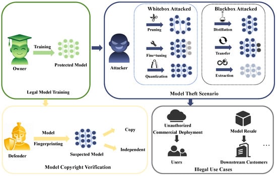
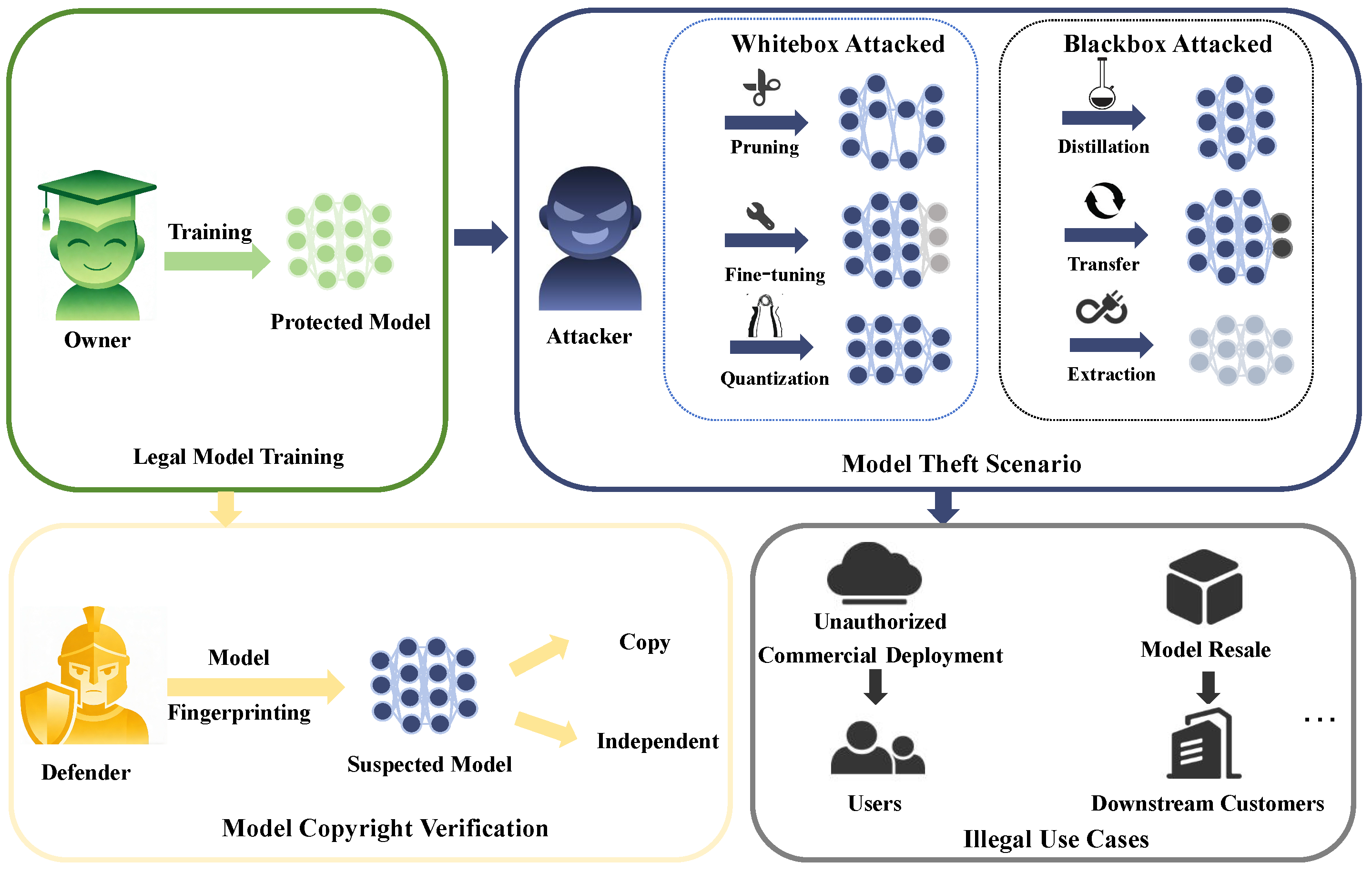
In recent years, deep neural network technology has developed rapidly, with increasingly innovative model architectures emerging and finding ever-wider applications. However, training a mature and deployable model often requires researchers to invest substantial expertise, as well as significant computational resources and time. Deep neural networks represent not only the intellectual property of researchers but also highly valuable commercial assets for enterprises. However, as shown in Figure 1, model owners train deep neural networks with intellectual property protection and apply them to downstream scenarios [1,2,3]. Due to the digital nature and easy dissemination of model parameters, and the continuous innovation of model reuse techniques such as fine-tuning [4], pruning [5,6], knowledge distillation [7,8,9], model extraction [10,11,12], and transfer learning [13,14], some malicious attackers illegally steal or copy unauthorized models for illicit profit. This severely infringes upon the intellectual property rights of researchers and poses a serious challenge to existing copyright protection mechanisms. Model theft not only violates the legitimate rights and interests of model owners but also seriously undermines the fairness of the artificial intelligence ecosystem [15].

Figure 1. The overview of model fingerprinting for copyright protection.

To safeguard researchers’ intellectual property rights and ensure the robust advancement of the artificial intelligence ecosystem, there is an imperative necessity to implement an efficient system for protecting model copyright. Model watermarking achieves model traceability by embedding unique identifiers or specific behavioral patterns [16], including white-box methods that rely on original network structures and black-box methods based on backdoor mechanisms [17]. However, watermarking methods face robustness challenges as embedded information can be destroyed during model modifications [18] and may affect the model’s original performance. Model fingerprinting, on the other hand, uses models’ natural behavioral traits to verify them without making any changes during training. Despite extensive research validating its feasibility, this technology continues to encounter numerous challenges in practical applications, including the sensitivity of decision boundary-based methods to model compression operations (such as pruning and quantization) [19], high false positive rates for independently trained models from the same source [20], and impractical requirements such as white-box access [21] or excessively high query counts and dataset requirements [22]. The aforementioned challenges and obstacles have also motivated us to consider more comprehensive and practical copyright protection methods.

Numerous studies have revealed that specific inputs lead to unique behavioral characteristics in models. Wang et al. [23] demonstrated that convolutional neural networks exhibit unique frequency domain responses to different frequency components. Geirhos et al. [24] showed that different training configurations result in significant differences in texture–shape bias. Furthermore, the loss function landscape study [25] showed that even using the same training data, neural networks converge to different local minima, thus forming unique decision boundary structures. The Mixup study [26] proposed that inter-class interpolation samples can reveal model-specific geometric structures in the feature space. These findings inspired us to design a multi-dimensional probing strategy that utilizes frequency sensitivity, decision boundary features, and inter-class behavioral patterns as complementary feature sources, combined with multi-level perturbation responses, to capture the unique dynamic behavioral characteristics of the model.

Based on the above research and insights, this paper proposes ProbeSpec, a black-box model fingerprinting method based on dynamic perturbation response spectrum analysis. ProbeSpec comprises three main components: multi-type probe generation (Gabor textures, boundary samples, and cross-class mixup samples) for comprehensive coverage of model behavioral space; multi-level perturbation response acquisition to construct dynamic trajectory response matrices; and 2D-DCT-based spectral fingerprint extraction for efficient feature compression. We conducted extensive experiments on six model architectures and four datasets. The results demonstrate that ProbeSpec can accurately identify various types of stolen models with only 80 queries, achieving extremely low false positive rates for independently trained homologous models. Even under strict conditions where only hard-label output is available, it achieves good results.

In summary, the main contributions of this paper are as follows:

• We propose a multi-dimensional complementary fingerprint probing strategy (Gabor texture, decision boundary, and cross-class mixup) that systematically captures model-specific behavioral patterns persisting after model modifications, achieving over 95% detection accuracy across all tested image classification architectures. Preliminary experiments demonstrate that this method can be extended to the text domain, achieving 93.59% accuracy on TinyBERT [27] models;
• We introduce the dynamic perturbation response spectrum as a fingerprint representation. Unlike existing methods that rely on static output matching or single-point boundary features, ProbeSpec captures behavioral trajectories across multiple perturbation levels, requiring only 80 queries (significantly fewer than methods like ZEST) while achieving an AUC greater than 0.97 across six architectures and maintaining extremely low false positive rates for independently trained models;
• The entire method operates under black-box access with label-only output. Even under this restricted setting, it achieves an AUC above 0.97, demonstrating practical deployment value for real-world copyright verification scenarios.

2. Related Work

Researchers are increasingly exploring model compression and transfer learning techniques for model reuse, driven by the continuous enhancement of model capabilities and the evolving range of application scenarios. However, this process also provides opportunities for attackers to illegally appropriate models, complicating the protection of intellectual property rights associated with these models. Current research primarily focuses on two categories of defense techniques: model watermarking, which incorporates specific identifiers or trigger sets during the training phase to assert copyright, and model fingerprinting, which involves extracting and analyzing the intrinsic features of the model to enhance identity recognition and verification capabilities [28].

2.1. Model Watermarking

Model watermarking technology achieves intellectual property protection by embedding specific identifiers or adjusting model parameters during the training phase. Based on access permissions, these techniques can be divided into two main categories: white-box watermarking and black-box watermarking methods. White-box watermarking methods require execution in a white-box environment, meaning that defenders must have full access to the model parameters—a limitation that severely restricts their application in real-world deployment scenarios. In contrast, black-box watermarking methods construct specialized watermark datasets through parameter tuning and utilize adversarial examples or backdoor attacks to achieve copyright verification under black-box conditions.

In the technical advancement of watermarking, initial methodologies were predominantly founded on adversarial examples and backdoor attack strategies. Jia et al. [29] put forward the Adv-watermark method, which combines watermarking techniques with adversarial algorithms to protect image copyright. Yan et al. [30] introduced OFSW, which integrates watermarks into an orthogonal feature space with regularization constraints to reduce task interference. Wang et al. [31] proposed a WPC-based DNN watermarking scheme that employs optimized probabilistic selection to differentiate key parameters from non-essential ones, facilitating high-fidelity and tamper-resistant copyright protection. Researchers have suggested more advanced technical solutions to make watermarks more secure and strong. Tan et al. [32] developed the SSW method, which creates adaptive trigger sets by optimizing paired symmetric shadow models, thus enhancing defense against model extraction attacks. Luo et al. [33] employed ACGAN to produce ephemeral trigger samples, successfully thwarting evidence leakage attacks in the verification phase. Ye et al. [34] employed deep hiding techniques to encode copyright information into trigger patterns and utilized triplet loss to enhance model recognition performance. Mo et al. [35] utilized DWT-DCT-SVD methodologies to integrate encrypted fingerprint watermarks into training data, thereby attaining black-box protection. Adorante et al. [36] put forward Opt-FreeMark, a post-training white-box watermarking technique that uses SVD and error-correcting codes to make small neural networks on edge devices more stable.

Despite the continuous advancement of model watermarking techniques, several challenges remain. As an intrusive copyright protection method, model watermarking inevitably affects model performance. When confronting increasingly sophisticated model stealing techniques, watermark information is susceptible to corruption or removal, leading to the failure of copyright verification.

2.2. Model Fingerprinting

Model fingerprinting creates unique identifiers by using non-intrusive methods to find unique features of models. Model fingerprinting is mainly divided into static and dynamic fingerprinting. Static fingerprinting generates identifiers based on fixed features or parameters of the model. For example, fingerprints can be generated by calculating the hash value of model parameters or by finding patterns in the parameter distribution of specific network layers. Although these methods are simple to use and computationally inexpensive, they are less robust. Dynamic fingerprinting captures the behavioral characteristics of the model during its operation as an identity identifier [37]. For instance, decision boundary-based methods exploit the unique characteristics of model decision boundaries. Cao et al. [38] put forward the IPGuard system, which uses data points close to decision boundaries as fingerprint features. However, single-point boundary samples are vulnerable to removal attacks. Adversarial perturbation-based methods leverage adversarial examples as fingerprints. Wang et al. [39] proposed fingerprinting using Universal Adversarial Perturbations (UAPs) to capture global decision boundary characteristics. Zhang et al. [40] applied adversarial fingerprinting in the text domain using the Fast Gradient Sign Method. These methods show good transferability but typically rely on gradient-based adversarial attacks, limiting their applicability in gradient-free black-box scenarios.

Dynamic perturbation-based methods represent a closely related approach to our work. DeepTaster [41] proposes a DNN fingerprinting method based on adversarial perturbation and frequency domain analysis. It detects whether a model uses a specific dataset by analyzing the statistical characteristics of adversarial examples in the DFT domain. However, gradient-based perturbations require white-box access or substitute models, and DFT analysis treats all frequency components equally without leveraging the energy compaction property. The ADV-TRA method [42] uses adversarial trajectories with dynamically adjusted step sizes to verify model ownership. Although it also uses dynamic perturbations, its focus is on generating trajectories through iterative boundary detection rather than performing perturbation response analysis of the system, and it requires a large query overhead. Furthermore, our DCT-based spectral analysis naturally concentrates energy in low-frequency coefficients, enabling more compact and discriminative fingerprint extraction. The multi-type probe design (frequency gradient, decision boundary, and cross-class samples) provides complementary perspectives on model behavior, whereas existing methods typically rely on a single probe type.

While the aforementioned studies focus on the image domain, the protection of large language models (LLMs) has also become a significant research hotspot due to their widespread deployment and substantial commercial value. Comprehensive investigations have systematically examined backdoor threats in LLMs, covering attack vectors in the pre-training, fine-tuning, and inference stages, as well as corresponding defense mechanisms and evaluation methods [43]. Current research has addressed potential threats such as data poisoning, hint injection, and jailbreak attacks, and has explored corresponding defense techniques in depth [44]. Attackers may exploit these security vulnerabilities to steal or tamper with protected models, thereby closely linking them to intellectual property protection. To address these challenges, researchers have proposed various protection methods specifically for LLMs. For example, Xu et al. [45] proposed an instruction fingerprinting method that embeds verifiable signatures through instruction tuning. Furthermore, recent research [46] has explored backdoor attacks and defense mechanisms from a fine-tuning perspective, providing new insights into LLM protection during model adaptation. Although our current focus is on image classification models, the principle of dynamic perturbation response analysis used by ProbeSpec lays the potential foundation for extending it to LLM fingerprint recognition, as demonstrated by our preliminary experiments in the text domain (see Section 4.6).

Despite the increasing number of fingerprinting methods being proposed, existing methods still face challenges such as high query overhead due to iterative optimization or extensive sampling, vulnerability to fine-tuning attacks that alter decision boundaries, and reliance on gradient information or white-box access. In contrast, ProbeSpec, through its complementary multi-type probe design combined with multi-level perturbation response spectrum analysis, achieves effective verification in a completely black-box setting with a small number of probes, while demonstrating superior robustness to model modifications.

3. Method

This part goes into detail about how the proposed ProbeSpec method will be put into action. ProbeSpec is a method for fingerprinting black-box models that uses dynamic perturbation response spectrum analysis. It gives a full picture of the model’s fingerprint from a dynamic point of view by making three types of probe samples and using the model’s behavioral patterns under perturbation conditions as unique identity markers.

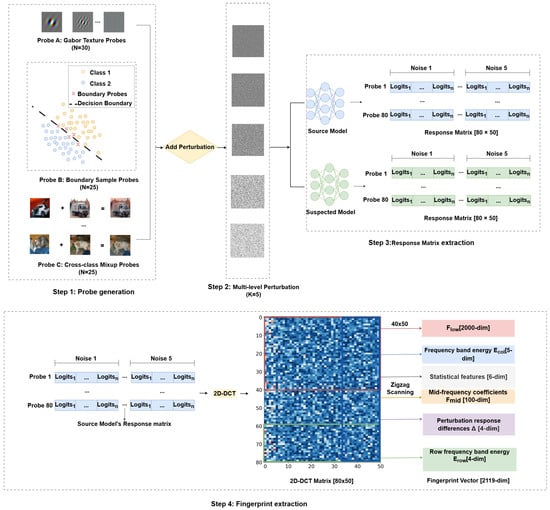
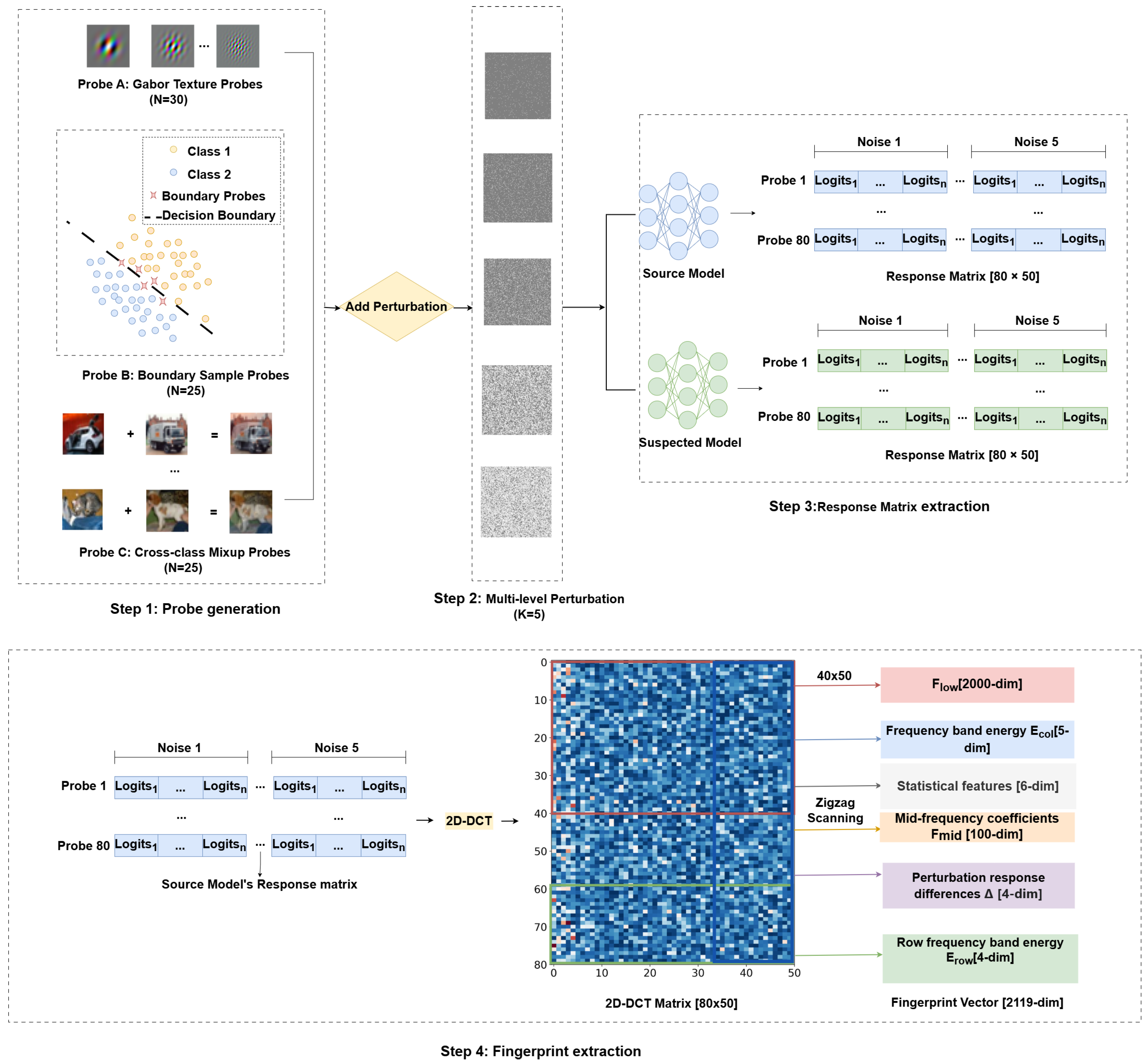
Regarding probe design, ProbeSpec employs three complementary types of probe samples to construct a comprehensive probing system: frequency gradient images to detect the model’s sensitivity to different spatial frequencies; decision boundary samples to capture the model’s predictive behavior characteristics for uncertain inputs; and cross-class mixup samples to elicit the model’s inter-class generalization responses. For fingerprint extraction, ProbeSpec uses a multi-level perturbation mechanism to collect the model’s response matrix, thereby obtaining more representative and stable information as a unique fingerprint. Finally, a feature extraction strategy incorporating multi-scale features is used to extract six complementary feature types from the DCT coefficient matrix, generating a more compact and identity-rich fingerprint vector. Figure 2 illustrates the overall framework of ProbeSpec: from multi-type probe sample generation to multi-level perturbation response collection, followed by frequency-domain transformation and feature extraction, ultimately achieving model ownership determination based on similarity thresholds.

Figure 2. Framework of ProbeSpec. ProbeSpec first generates three probe types (frequency gradient, decision boundary, and cross-class mixup samples), then applies multi-level perturbations to collect response matrices, and finally extracts six complementary DCT features to form compact fingerprints.

3.1. Multi-Type Probe Sample Generation

The rational design of probe samples is crucial to model fingerprinting methods. This section provides a detailed description of the three functionally complementary types of probe samples constructed by ProbeSpec, which probe model behavior from three dimensions: frequency response characteristics, decision boundary sensitivity, and cross-class generalization behavior.

3.1.1. Type A Probe: Frequency Gradient Image

Deep neural networks exhibit distinct response characteristics to inputs of varying spatial frequencies [23]. Research has demonstrated that convolutional neural networks tend to learn textural features rather than shape features from images, and different training processes lead to variations in model sensitivity to different frequency components [24]. Based on this observation, we design Type A probes aimed at systematically probing the model’s response patterns to different spatial frequencies and utilizing these as fingerprint information.

Leveraging the favorable localization properties of Gabor filters in both frequency and spatial domains [47], we employ them to generate 30 synthetic texture images at different frequencies as probe samples. The frequency parameters are configured to span from low to high frequency ranges, enabling systematic probing of the model’s spectral response characteristics. The mathematical definition of the two-dimensional Gabor function is as follows:

$$G(x,y;f,\theta ,\sigma )=exp\left(-{\displaystyle \frac{{x^{\prime }}^2+{y^{\prime }}^2}{2{\sigma }^2}}\right)·cos\left(2\pi f{x}^{\prime }\right),$$

(1)

where the coordinate transformation is defined as follows: $x^{\prime }=xcos\theta +ysin\theta$ and $y^{\prime }=-xsin\theta +ycos\theta$, f denotes the spatial frequency, $\theta$ the orientation angle, and $\sigma$ the standard deviation of the Gaussian envelope. By adjusting these parameters, synthetic texture images with different frequency and orientation characteristics can be generated.

In our experiments, we uniformly select 6 frequency values within the frequency range $f\in [0.05,0.4]$ and 5 orientation angles within the direction range $\theta \in [0,\pi ]$, generating diverse Gabor textures through their combinations. To produce three-channel RGB images, we apply slight phase offsets ${\varphi }_c=c·\pi /6$ (where $c\in \{0,1,2\}$ corresponds to the R, G, and B channels, respectively) to each channel, thereby ensuring consistency in frequency characteristics while maintaining diversity among the probe samples. All generated texture images are resized to the target dimensions (e.g., $32\times 32$ for CIFAR-10) and normalized according to the statistical properties (mean and standard deviation) of the target dataset, ensuring that the numerical range of inputs is consistent with the training data.

3.1.2. Type B Probe: Decision Boundary Sample

Decision boundaries are inherent characteristics formed by deep neural networks during training, depending on various factors including data distribution, network architecture, optimization algorithms, and random initialization. Even for two models independently trained on the same dataset, subtle differences exist in the fine-grained structure of their decision boundaries. Type B probes utilize samples located near the decision boundaries to probe the model’s boundary characteristics as fingerprint features.

Given the source model $f_s$ and the test dataset ${\mathcal{D}}_{test}$, we select Type B probes through the following procedure: First, for each sample x in the test set, we compute the model’s Softmax prediction probability distribution $p\left(x\right)=\mathrm{Softmax}\left(f_s\left(x\right)\right)$ and obtain the maximum confidence $c_{max}\left(x\right)={max}_k{p}_k\left(x\right)$ along with the predicted class $\widehat{y}\left(x\right)=\arg {\max }_k{p}_k\left(x\right)$. Subsequently, samples satisfying the following conditions are selected to constitute the Type B probe set:

$${\mathcal{P}}_B=\{x\in {\mathcal{D}}_{test}\mid {\tau }_l\le c_{max}\left(x\right)\le {\tau }_h\wedge \widehat{y}\left(x\right)=y\left(x\right)\},$$

(2)

where ${\tau }_l$ and ${\tau }_h$ denote the lower and upper bounds of confidence, respectively, and $y\left(x\right)$ represents the ground-truth label of the sample. In our experiments, the default settings are ${\tau }_l=0.5$, ${\tau }_h=0.85$. The bounds ${\tau }_l=0.5$ and ${\tau }_h=0.85$ ensure selected samples lie near decision boundaries with moderate uncertainty while being correctly classified. This design leverages the fact that stolen models inherit decision boundary characteristics from the source model, whereas independently trained models exhibit distinct boundary structures, thereby enabling differentiation of model provenance.

3.1.3. Type C Probes: Cross-Class Mixed Samples

Type C probes generate mixed samples spanning different classes through linear interpolation [26]. These samples probe the geometric structure and decision boundary morphology of the model in high-dimensional feature space. Research has demonstrated that even when trained on identical data, different models converge to different local minima in the loss landscape, resulting in significantly different behavioral patterns in inter-class regions [25]. Stolen models, by inheriting the source model’s parameters, retain its response characteristics on inter-class manifolds, making cross-class mixed samples an effective tool for model fingerprinting.

Given two samples $x_i$ and $x_j$ from different classes i and j (where $i\ne j$), the mixed sample is generated through the following Mixup operation:

$$x_{mix}=\alpha ·x_i+(1-\alpha )·x_j,$$

(3)

where $\alpha \in (0,1)$ is the interpolation coefficient that controls the contribution ratio of the two source samples to the mixed sample.

For a classification task with K classes, there exist $\left({\displaystyle \genfrac{}{}{0pt}{}{K}{2}}\right)=K(K-1)/2$ class pairs, each representing a specific inter-class relationship with varying semantic similarity (e.g., “cat-dog” vs. “cat-car”). To systematically generate Type C probes, we randomly select $M=20$ representative samples per class from the test set. For each class pair, we generate mixed samples using three interpolation coefficients $\alpha \in \{0.3,0.5,0.7\}$, and the final $N_C$ probes are obtained through random subsampling from these candidates.

3.1.4. Probe Combination Strategy and Configuration

Based on the detailed description of the three types of probes above, the final probe set $\mathcal{P}$ is composed of the union of the three probe categories:

$$\mathcal{P}={\mathcal{P}}_A\cup {\mathcal{P}}_B\cup {\mathcal{P}}_C.$$

(4)

Specifically, Type A probes capture low-level frequency features, Type B probes detect mid-level decision boundaries, and Type C probes reveal high-level semantic relationships, thereby achieving multi-scale feature coverage. In the default experimental configuration, we set $|{\mathcal{P}}_A|=30$ (30 frequency gradient probes), $|{\mathcal{P}}_B|=25$ (25 boundary probes), and $|{\mathcal{P}}_C|=25$ (25 mixed probes), totaling $\left|\mathcal{P}\right|=80$ probe samples. This configuration achieves a favorable balance among detection effectiveness, computational efficiency, and robustness. Subsequent ablation experiments (Section 4) will validate the contribution of each probe type and the impact of probe quantity on detection performance.

3.2. Multi-Level Perturbation Response Acquisition

For each probe sample $x\in \mathcal{P}$, we construct perturbed samples by adding Gaussian noise:

$${\tilde{x}}_{\sigma }=x+ϵ,ϵ\sim \mathcal{N}(0,{\sigma }^{2}I),$$

(5)

where $\sigma$ denotes the perturbation intensity, and I is the identity matrix with the same dimensions as the input. The perturbation intensity $\sigma$ is selected from a predefined set of levels $\mathcal{S}$. In the default configuration, we employ five perturbation levels: $\mathcal{S}=\{0,0.05,0.1,0.15,0.2\}$. To prevent pixel values from exceeding valid ranges after perturbation, we apply clipping to the perturbed samples:

$${\tilde{x}}_{\sigma }=\mathrm{clamp}({\tilde{x}}_{\sigma },x_{min},x_{max}),$$

(6)

where $x_{min}$ and $x_{max}$ denote the minimum and maximum values of the normalized input, respectively. Through the multi-level perturbation mechanism, we can observe the trajectory of model responses as perturbation intensity varies. This dynamic variation pattern constitutes the model’s unique “behavioral signature.”

For each perturbed probe sample ${\tilde{x}}_{\sigma }$, we query the target model to obtain its raw output (logits) $z=f\left({\tilde{x}}_{\sigma }\right)\in {\mathbb{R}}^K$, where K is the number of classes. To enhance the discriminability of fingerprints and ensure cross-model comparability, we apply z-score normalization to standardize the logits:

$$\widehat{z}={\displaystyle \frac{z-{\mu }_z}{{\sigma }_z+ϵ}},$$

(7)

where ${\mu }_z={\displaystyle \frac{1}{K}}{\sum }_{k=1}^K{z}_k$ is the mean of the logits vector, ${\sigma }_z=\sqrt{{\displaystyle \frac{1}{K}}{\sum }_{k=1}^K{(z_k-{\mu }_z)}^2}$ is the standard deviation, and $ϵ={10}^{-8}$ is a small constant to prevent division by zero.

After collecting the normalized logits responses of all probes across all perturbation levels, we proceed to generate the perturbation response matrix. Let the probe set size be $N=\left|\mathcal{P}\right|$, the number of perturbation levels be $M=\left|\mathcal{S}\right|$, and the number of classes be K. The response matrix $\mathbf{R}$ is constructed as follows:

For probe $x_i$ and perturbation level ${\sigma }_j$, let ${\widehat{\mathbf{z}}}_{i,j}\in {\mathbb{R}}^K$ denote the normalized logits vector. We horizontally concatenate the responses of the same probe across all perturbation levels to form the complete response vector for that probe:

$${\mathbf{r}}_i=[{\widehat{\mathbf{z}}}_{i,1};{\widehat{\mathbf{z}}}_{i,2};\dots ;{\widehat{\mathbf{z}}}_{i,M}]\in {\mathbb{R}}^{K·M}.$$

(8)

By vertically stacking the response vectors of all probes, we obtain the perturbation response matrix:

$$\mathbf{R}=\left[\begin{array}{c}{\mathbf{r}}_1^T\\ {\mathbf{r}}_2^T\\ ⋮\\ {\mathbf{r}}_N^T\end{array}\right]\in {\mathbb{R}}^{N\times (K·M)}.$$

(9)

3.3. Spectral Fingerprint Extraction

The perturbation response matrix $\mathbf{R}$ contains rich behavioral information but exhibits high dimensionality and redundancy. To efficiently extract fingerprint information, we apply the two-dimensional discrete cosine transform (2D-DCT) to transform the response matrix:

$$\mathbf{D}={\mathrm{DCT}}_{\mathrm{col}}\left({\mathrm{DCT}}_{\mathrm{row}}\left(\mathbf{R}\right)\right),$$

(10)

where ${\mathrm{DCT}}_{\mathrm{row}}$ and ${\mathrm{DCT}}_{\mathrm{col}}$ denote DCT applied along rows and columns, respectively. After the transformation, the coefficient matrix $\mathbf{D}\in {\mathbb{R}}^{N\times (K·M)}$ preserves the same dimensions as $\mathbf{R}$, with low-frequency coefficients concentrated in the upper-left region representing overall behavioral patterns, and high-frequency coefficients in the lower-right region corresponding to fine-grained details.

To construct robust and compact fingerprints, we extract six complementary feature types from the DCT coefficient matrix, as illustrated in Table 1. The complete fingerprint extraction procedure is detailed in Algorithm 1.

Algorithm 1: ProbeSpec Fingerprint Extraction

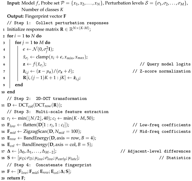Table 1. Fingerprint feature components and their dimensions under the default configuration ($N=80$ probes, $K=10$ classes, and $M=5$ perturbation levels).

Component	Description	Formula	Dim
${\mathbf{F}}_{low}$	Low-frequency coefficients	$r_l\times c_l$	2000
${\mathbf{F}}_{mid}$	Mid-frequency coefficients	$N_{mid}$	100
${\mathbf{E}}_{row}$	Row-wise band energies	$B_{row}$	4
${\mathbf{E}}_{col}$	Column-wise band energies	$B_{col}$	5
$\Delta$	Perturbation response differences	$M-1$	4
$\mathbf{S}$	Statistical features	-	6
Total			2119

Low-frequency coefficients. We extract coefficients from the upper-left $r_l\times c_l$ rectangular region of the DCT matrix, where $r_l=min(\lfloor N/2\rfloor ,40)$ and $c_l=min(K·M,50)$. These coefficients contain the principal energy and capture the dominant response patterns. The extracted region is flattened to form ${\mathbf{F}}_{low}\in {\mathbb{R}}^{r_l·c_l}$. The $40\times 50$ region is chosen to capture the majority of total DCT energy while excluding high-frequency noise components that vary with random perturbations.

Mid-frequency coefficients. To capture supplementary detail information beyond the low-frequency region, we employ the classical Zigzag scanning strategy [48] to select $N_{mid}=100$ additional coefficients in order of increasing frequency. This scanning pattern naturally orders coefficients from low to high frequency along diagonal traversals, ensuring that the most informative mid-frequency components are preserved while keeping the total fingerprint dimension manageable.

Frequency band energy. We partition the DCT matrix into frequency bands and compute the normalized energy distribution as auxiliary features. Specifically, we divide the matrix into $B_{row}=4$ bands along the row direction and $B_{col}=min(5,\lfloor C/10\rfloor )$ bands along the column direction. The band numbers are chosen to provide sufficient granularity for energy distribution analysis while keeping the feature dimension low ($4+5=9$ dimensions). The energy of the b-th band is computed as follows:

$$E_b={\displaystyle \frac{{\sum }_{(i,j)\in {\mathcal{B}}_b}{D}_{i,j}^2}{{\sum }_{i,j}{D}_{i,j}^2+ϵ}},$$

(11)

where $D_{i,j}$ denotes the element at row i and column j of the DCT matrix $\mathbf{D}$, ${\mathcal{B}}_b$ is the index set of the b-th frequency band, and $ϵ={10}^{-10}$ prevents division by zero. Row-wise band energies ${\mathbf{E}}_{row}$ reflect response intensity distribution across different probe types, while column-wise energies ${\mathbf{E}}_{col}$ capture the model’s sensitivity distribution across perturbation levels.

Perturbation response differences. To explicitly capture behavioral variations across perturbation levels, we compute the mean absolute difference of DCT coefficients between adjacent perturbation blocks:

$${\Delta }_j={\displaystyle \frac{1}{N·K}}\sum _{i=1}^N\sum _{k=0}^{K-1}\left|D_{i,(j+1)K+k}-D_{i,jK+k}\right|,$$

(12)

where $j=0,1,\dots ,M-2$ indexes pairs of adjacent perturbation levels. This feature directly quantifies how rapidly model responses change as perturbation intensity increases, providing discriminative information for distinguishing stolen models from independent ones.

Statistical features. Finally, we compute six global statistics from the DCT matrix: overall mean ${\mu }_D$, overall standard deviation ${\sigma }_D$, low-frequency region mean ${\mu }_{low}$ (computed over the upper quarter of rows), low-frequency region standard deviation ${\sigma }_{low}$, mean of the first half columns ${\mu }_{early}$ (corresponding to low perturbation responses), and mean of the second half columns ${\mu }_{late}$ (corresponding to high perturbation responses). These statistics provide a macroscopic characterization of the response distribution:

$$\mathbf{S}=[{\mu }_D;{\sigma }_D;{\mu }_{low};{\sigma }_{low};{\mu }_{early};{\mu }_{late}].$$

(13)

The final fingerprint $\mathbf{F}$ is formed by concatenating all feature components:

$$\mathbf{F}=[{\mathbf{F}}_{low};{\mathbf{F}}_{mid};{\mathbf{E}}_{row};{\mathbf{E}}_{col};\Delta ;\mathbf{S}]\in {\mathbb{R}}^{d_F},$$

(14)

where $d_F=2119$ under the default configuration. This represents a compression ratio of approximately 53% compared to the original response matrix ($80\times 50=4000$ elements), while preserving the discriminative information essential for model identification.

4. Experiments and Results

4.1. Experimental Setup

4.1.1. Datasets

This study employs four widely-used image classification benchmark datasets to evaluate the performance of ProbeSpec. CIFAR-10 and CIFAR-100 [49] each contain 60,000 color images of 32 × 32 pixels, with 10 and 100 classes, respectively, comprising 50,000 training images and 10,000 test images. The SVHN (Street View House Numbers) [50] dataset consists of over 600,000 digit images of 32 × 32 pixels captured from real-world street views. ImageNet-100 [51], a subset of ImageNet-1K, contains 100 classes with images at a resolution of 224 × 224 pixels.

4.1.2. Protected Model Architectures

This study selects six representative deep neural network architectures as source models: ResNet-50, ResNet-34 [52], DenseNet-169 [53], EfficientNet-B0 [54], MobileNetV2 [55], and InceptionV3 [56]. These models encompass diverse architectural types, including residual networks, densely connected networks, efficient networks, lightweight networks, and multi-scale feature extraction networks, ensuring comprehensive and representative evaluation.

4.1.3. Model Pool Construction

For each source model architecture, we construct a model pool containing stolen models and independent models. Stolen models are generated through the following five categories of model stealing attacks:

Fine-tuning: Various fine-tuning strategies with different depths are employed, including last-layer fine-tuning, last-block fine-tuning, half-network fine-tuning, low-learning-rate full-network fine-tuning, and progressive unfreezing [4].

Pruning: Three pruning methods are applied (improved unstructured pruning, layer-sensitive pruning [5], and progressive pruning [6]), combined with six sparsity ratios (ranging from 5% to 30%) and multiple random seeds.

Knowledge Distillation: Knowledge Distillation [7] transfers dark knowledge through softened probability distributions; Attention Transfer [8] aligns spatial attention maps between teacher and student models; Relational Knowledge Distillation [9] preserves distance and angular relationships among samples.

Model Extraction: Knockoff Nets [10] queries target model API with surrogate datasets to train clone models; JBDA [11] generates synthetic samples via Jacobian matrices to approximate decision boundaries; ActiveThief [12] combines active learning with adversarial sample selection to optimize query efficiency.

Transfer Learning: Feature Extraction Transfer [13] freezes feature extraction layers and trains only the classifier; Fine-tuning Transfer [14] performs end-to-end fine-tuning with source model weights as initialization.

Independent models are primarily constructed through the following: training the same architecture on partial data subsets; training the same architecture with different random seeds and optimizers; training different architectures on the same complete dataset; and training different architectures on different datasets.

In our experiments, the evaluation encompasses a total of 544 models across all source models.

4.1.4. Evaluation Metrics and Implementation Details

We adopt six metrics for comprehensive evaluation: accuracy for overall classification performance; false positive rate (FPR) for measuring false accusations; recall for detection sensitivity; F1 score for balanced performance; ROC-AUC for overall discrimination capability; and verification time for computational efficiency. All experiments were implemented using PyTorch 2.0.1 and Python 3.9.13. The models were trained and evaluated on an NVIDIA Tesla V100 GPU (NVIDIA Corporation, Santa Clara, CA, USA) with CUDA 11.7.

4.2. Performance Evaluation and Comparison

To validate the effectiveness of ProbeSpec, we compare it with four representative model fingerprinting methods: ZEST [37], SAC-W [57], SAC-JC [58], and MetaFinger [59]. Experiments are conducted on two architectures, ResNet-50 and MobileNetV2, with a model pool containing 197 models in total. To ensure a fair comparison, all methods are evaluated under identical hardware configurations and unified evaluation protocols.

Table 2 shows that ProbeSpec does the best job on all of the evaluation metrics. ProbeSpec’s identification accuracy is 96.45%, which is 17.1 percentage points better than the best baseline method, MetaFinger. ProbeSpec’s false positive rate is only 3.13%, which is much lower than all of the baseline methods. Our independent models pool has a lot of homologous models that are likely to be misclassified. For example, models with the same architecture that were trained separately. ProbeSpec’s very low false positive rate in these difficult conditions shows that it can be trusted in real-world situations. ProbeSpec also gets an F1 score of 96.52% and a recall of 96.04%. This means that the method strikes a good balance between precision and recall, keeping false positives to a minimum while still finding a lot of things.

Table 2. Comparison with baseline methods. Best results are in bold.

Method	Accuracy ↑ (%)	FPR ↓ (%)	F1 ↑ (%)	Recall ↑ (%)	Time (s)
ZEST	76.77	36.05	78.05	92.75	981.00
SAC-W	74.19	30.00	80.00	76.19	132.60
SAC-JC	63.87	47.50	67.06	76.00	1.15
MetaFinger	79.35	29.41	82.42	85.21	177.60
ProbeSpec (Ours)	96.45	3.13	96.52	96.04	0.68

In terms of computational efficiency, ProbeSpec also exhibits significant advantages. As shown in the last column of Table 2, ProbeSpec requires only 0.68 s to complete a single model verification, which is $1.7\times$, $195\times$, $261\times$, and $1443\times$ faster than SAC-JC, SAC-W, MetaFinger, and ZEST, respectively. This efficiency advantage stems from the lightweight design of ProbeSpec: fingerprint extraction requires only 80 model queries, without the need for iterative optimization or adversarial example generation. In contrast, ZEST requires $O(N\times L)$ queries for N reference points across L network layers to compute layer-wise representations [37], while MetaFinger involves computationally expensive meta-learning procedures [59]. The advantages of low query overhead and high detection accuracy make ProbeSpec more valuable for practical deployment.

To validate the effectiveness of ProbeSpec, we conducted extensive testing under different attack scenarios. Table 3 presents the detailed composition of the model pool and the detection performance for each category. The model pool comprises 544 models in total: 275 stolen models (covering five attack types) and 269 independent models (covering three categories). Experiments demonstrate that ProbeSpec achieves a 0% false negative rate in identifying white-box attacks (fine-tuning and pruning), which is theoretically reasonable since these attacks preserve most model parameters. Under black-box attack scenarios, the proposed method achieves a detection accuracy of 100% against distillation attacks and detection accuracies of 94.87% and 95.12% against extraction attacks and transfer attacks, respectively (with false positive rates of 5.13% and 4.88%). This result is consistent with expectations, as black-box attacks can only obtain model outputs via API calls, and attackers lack direct access to the internal architecture of the model, leading to increased attack difficulty and a corresponding decline in detection performance.

Table 3. Fine-grained detection performance across attack types and independent model categories. FNR: false negative rate (missed stolen models). FPR: false positive rate (independent models incorrectly flagged as stolen).

Category	Model Type	Count	Accuracy	FNR/FPR (%)
Stolen Models	Fine-tuning	80	100%	0 (FNR)
	Pruning	74	100%	0 (FNR)
	Knowledge Distillation	41	100%	0 (FNR)
	Model Extraction	39	94.87%	5.13 (FNR)
	Transfer Learning	41	95.12%	4.88 (FNR)
Independent Models	Same Arch but Different Training Strategy	55	94.55%	5.45 (FPR)
	Different Data Subset	74	90.54%	9.46 (FPR)
	Different Hyperparameters or Dataset	140	100%	0 (FPR)

To comprehensively evaluate the robustness of our method, we constructed a diverse independent model pool, including the following: (1) same architecture and same dataset but different training strategies; (2) same architecture with partially overlapping datasets; (3) different architectures with the same dataset; (4) different architectures with different datasets. As shown in Table 3, for the latter two categories of independent models with greater differences (different architectures), ProbeSpec achieves a 0% false positive rate. For the first two categories of independent models, the false positive rates are 5.4% and 9.46%, respectively. This result is acceptable because these models share the same architecture as the source model and are trained on overlapping data, leading to high similarity in partial decision boundaries. Notably, these two cases represent a challenging edge scenario, yet ProbeSpec’s experimental results remain practically viable.

It should be noted that black-box attack samples (39–41 samples per type) are fewer than white-box attack samples (74–80 samples per type), primarily due to the high computational cost and difficulty of training surrogate models. Nevertheless, we ensured in our experimental design that the ratio of related models to unrelated models is approximately 1:1, thereby guaranteeing the scientific rigor and fairness of the experiments.

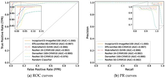
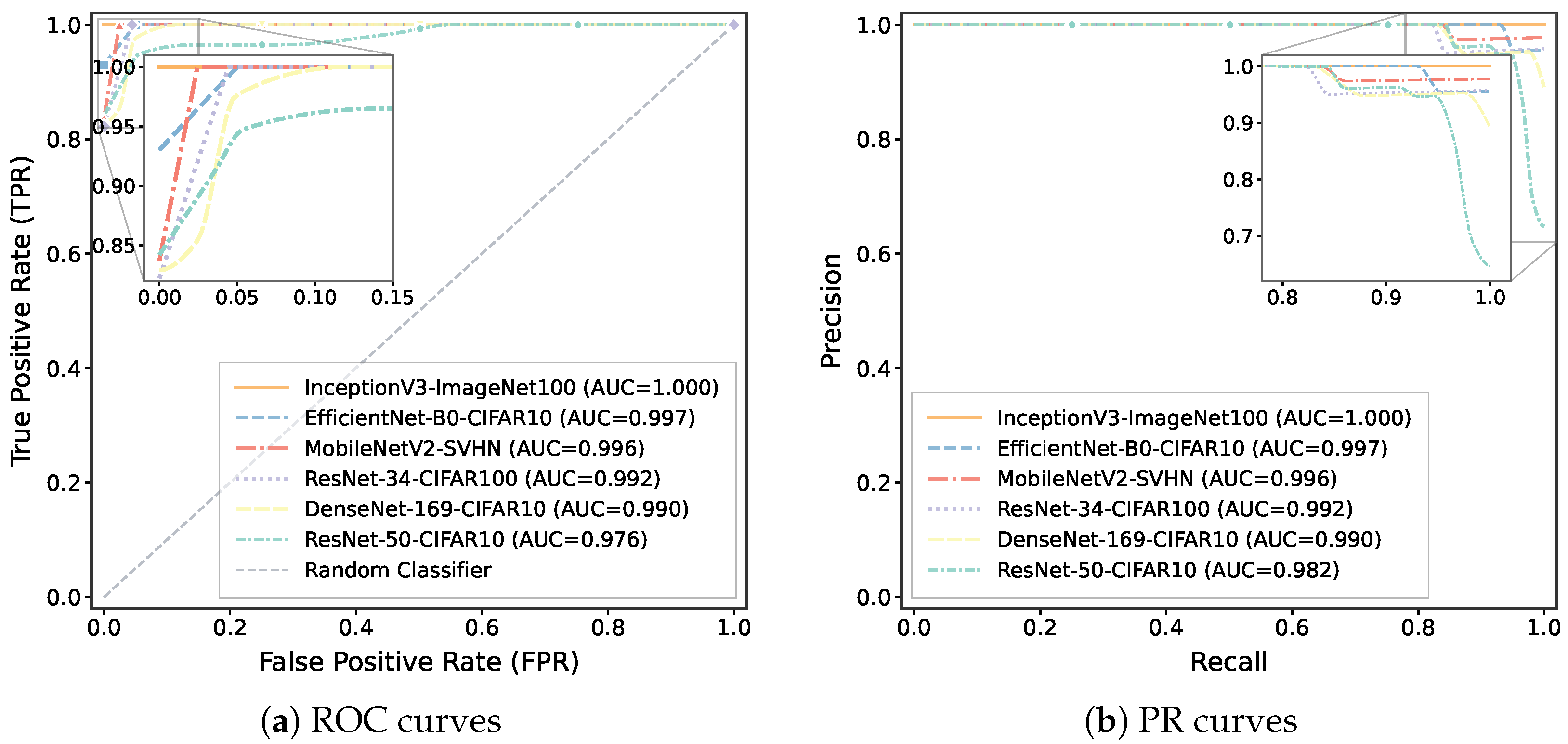
To specifically analyze the effectiveness of ProbeSpec across six architectures, as shown in Table 4, ProbeSpec successfully detects 100% of white-box plagiarism attacks (pruning and fine-tuning) across all architectures. For the more challenging black-box plagiarism attacks, the method still demonstrates excellent performance, with an overall accuracy exceeding 95%. Notably, it achieves 100% accuracy for all types of attacks on InceptionV3-ImageNet100. Figure 3 displays the ROC curves and precision–recall curves for all six source models. All models achieve ROC-AUC values above 0.976, with InceptionV3 reaching 1.000.

Table 4. Detection accuracy (%) across different architectures and attack types.

Source Model	Pruning	Fine-Tune	Transfer	Extract	Distill	Independent	Overall
ResNet-50	100	100	89	80	100	95	95
DenseNet-169	100	100	89	100	100	95	96
EfficientNet-B0	100	100	100	100	100	95	98
MobileNetV2	100	100	100	100	100	98	99
ResNet-34	100	100	100	100	100	98	98
InceptionV3	100	100	100	100	100	100	100

Figure 3. ROC and precision-recall curves for ProbeSpec evaluation.

4.3. Robustness Analysis

To evaluate the robustness of ProbeSpec in real-world deployment scenarios, we conducted tests from two aspects: (1) performance in a restricted API environment; and (2) resistance to adaptive attacks.

4.3.1. API Query Limitations

In practical application scenarios, we cannot obtain the complete logits output, but only the probability distribution or the predicted label. To verify the applicability of ProbeSpec in these restricted scenarios, we tested three output modes on six different architectures: (1) Logits: the complete output vector; (2) Probability: the probability distribution normalized by softmax; (3) Label-only: only the predicted class label is returned. As shown in Table 5, ProbeSpec maintained high detection performance under all three output modes. From complete logits to only probability distribution, the average ROC-AUC decreased from 0.992 to 0.972; when further restricted to only label output, the average ROC-AUC was 0.971. The overall performance degradation was no more than 2.1%, indicating that the core mechanism of ProbeSpec—fingerprint extraction based on perturbation response spectrum—does not heavily rely on the precise numerical values of the output, but rather captures the model’s behavior patterns under different perturbations. This result verifies the practicality of ProbeSpec in restricted API environments.

Table 5. ROC-AUC performance under different API output modes across six architectures. Logits: full output vectors; Probability: softmax probability distributions; Label-only: predicted class labels only.

Architecture	Logits	Probability	Label-Only
ResNet-50	0.976	0.951	0.943
DenseNet-169	0.990	0.952	0.958
MobileNetV2	0.996	0.964	0.962
EfficientNet-B0	0.997	0.983	0.984
InceptionV3	1.000	0.989	0.992
ResNet-34	0.992	0.990	0.989
Average	0.992	0.972	0.971

4.3.2. Adaptive Attack Resistance

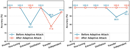
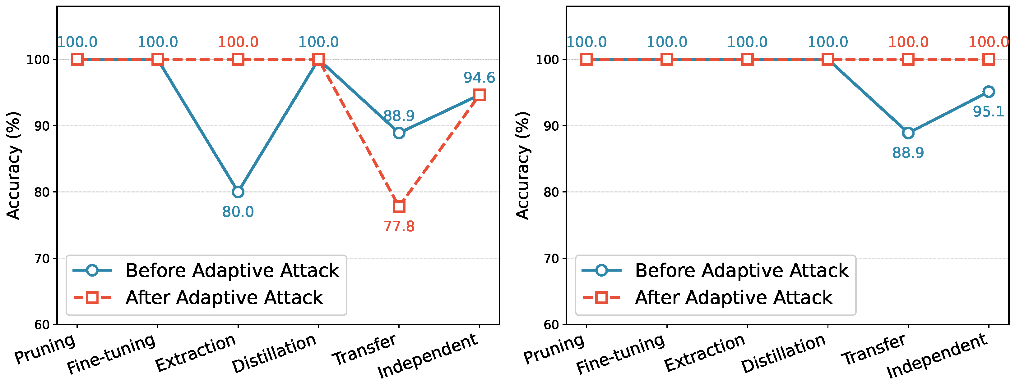
In practice, attackers might attempt to evade detection by altering the model’s response pattern to perturbations through noise-augmented fine-tuning. To verify ProbeSpec’s robustness against such adaptive attacks, we designed the following experiment: the stolen model was subjected to additional fine-tuning training, where 50% of the training samples had random Gaussian noise added (noise intensity $\sigma$ was randomly selected from 0.05, 0.1, 0.15, 0.2), for 5 epochs with a learning rate of 0.001. We performed adaptive attacks on stolen models of five attack types using two architectures, ResNet-50 and DenseNet-169, and re-extracted fingerprints for detection. As shown in Figure 4, the experimental results show that noise-augmented fine-tuning not only failed to effectively reduce the detection rate but actually increased it in most cases. For example, for model extraction attacks on ResNet-50, the detection rate increased from 80% to 100%; for transfer learning attacks on DenseNet-169, the detection rate increased from 88.9% to 100%. Only the transfer learning attack on ResNet-50 showed a decrease (88.9%→77.8%), but it still maintained acceptable detection capabilities.

Figure 4. Detection rates before and after adaptive attacks on ResNet-50 (left) and DenseNet-169 (right). Noise-augmented fine-tuning (5 epochs, $\sigma \in \{0.05,0.1,0.15,0.2\}$) fails to evade detection and paradoxically increases detection rates in most cases.

The experimental results show that although noise-augmented training changes the model’s local response to random noise, it also makes the model’s decision boundary smoother, thus enhancing its similarity to the source model in terms of macroscopic behavioral patterns. Furthermore, the diverse probe samples used by ProbeSpec make it difficult for attackers to evade all probe types simultaneously. These results demonstrate that ProbeSpec possesses inherent robustness against adaptive attacks.

4.4. Ablation Studies

ProbeSpec’s effectiveness was further validated through a comprehensive ablation study examining probe types, perturbation levels, and probe numbers.

4.4.1. Parameter Sensitivity Analysis

To validate the rationale of our probe design, we conducted comprehensive sensitivity analyses on each probe type’s key parameters using ResNet-50-CIFAR10 with 113 models (57 stolen across five attack types; 56 independent). Table 6 presents the results.

Table 6. Comprehensive parameter sensitivity analysis across three probe types on ResNet-50-CIFAR10 (113 models). Baseline: 30 Gabor + 25 Boundary [0.5, 0.85] + 25 Mixup [0.3, 0.5, 0.7]. Bold indicates optimal configuration.

Configuration	Acc	AUC	Fine	Prune	Black	Ind.FPR
	(%)		(%)	(%)	(%)	(%)
Type A
Gabor (Ours)	94.69	0.976	100	100	88.89	5.36
Checkerboard	92.04	0.963	100	100	85.19	8.93
Random Noise	87.61	0.894	100	93.3	67.86	8.93
Type B
[0.3, 0.7]	93.81	0.973	100	100	85.19	5.36
[0.4, 0.8]	93.81	0.974	100	100	85.19	5.36
[0.5, 0.85] (Ours)	94.69	0.976	100	100	88.89	5.36
[0.6, 0.9]	92.92	0.973	100	100	85.19	7.14
[0.7, 0.95]	93.81	0.974	100	100	85.19	5.36
Type C
Single [0.5]	92.92	0.972	100	100	70.37	0.00
Dual [0.3, 0.7]	92.92	0.973	100	100	85.19	7.14
Triple [0.3, 0.5, 0.7] (Ours)	94.69	0.976	100	100	88.89	5.36
Five [0.2, 0.35, 0.5, 0.65, 0.8]	92.92	0.972	100	100	85.19	7.14

Fine = Fine-tuning; Prune = Pruning; Black = Black-box attacks (distillation, transfer, and extraction); Ind.FPR = Independent model False Positive Rate.

Type A: Pattern Selection. We compared Gabor filters, checkerboard patterns, and random Gaussian noise as Type A probes. As shown in Table 6, Gabor filters achieved the highest overall accuracy (94.69%, ROC-AUC 0.976). Notably, Gabor significantly outperformed alternatives on black-box attacks (88.89% vs. 67.86% for random noise), demonstrating that frequency-domain sensitivity is critical for detecting black-box attacks.

Type B: Confidence Threshold. We evaluated five threshold pairs for boundary sample selection. Our [0.5, 0.85] configuration achieved the best black-box detection performance (88.89% vs. 85.19% for alternative ranges). Excessively wide ranges ([0.3, 0.7]) include samples too far from decision boundaries, reducing discriminability; excessively narrow ranges ([0.7, 0.95]) yield insufficient samples (∼15 vs. ∼25 per class), limiting boundary coverage.

Type C: Mixup Coefficients. We compared four coefficient configurations. Single-coefficient probing ($\alpha =0.5$ only) performed poorly on black-box attacks (70.37%), while our three-coefficient configuration $\alpha \in \{0.3,0.5,0.7\}$ achieved 88.89%. This demonstrates that the triple-coefficient design provides superior black-box attack detection through complementary manifold coverage.

4.4.2. Effect of Probe Types

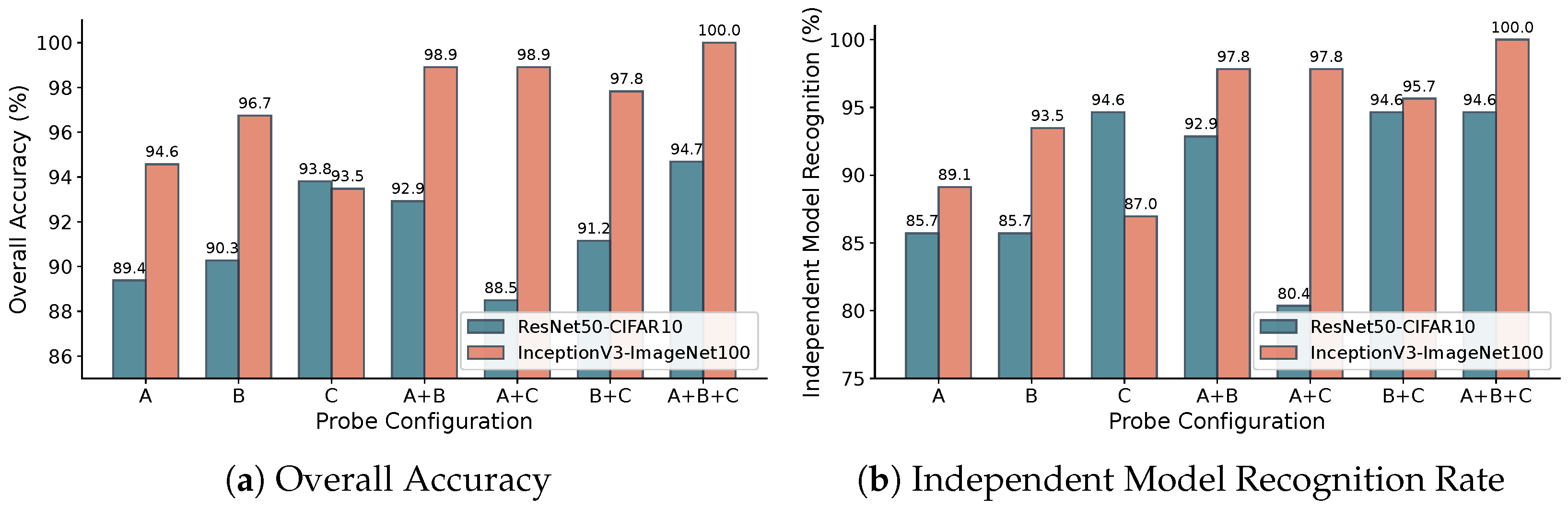
To confirm the effectiveness of the three-probe combination and examine the contribution of each probe type, we assessed seven probe configurations on the ResNet-50-CIFAR10 and InceptionV3-ImageNet100 datasets. Figure 5a shows the results. Type A probes represent Gabor patterns for capturing frequency-domain responses, Type B probes represent boundary samples sensitive to decision boundary variations, and Type C probes represent mixed samples for revealing cross-class transformation behavior. From the perspective of single probe types, each probe exhibits limitations in independent model recognition: on InceptionV3, the accuracy rates using three single probes were 94.6%, 96.7%, and 93.5%, all lower than the cases using dual and triple probes. This means that one type of probe cannot fully capture all of a model’s behavioral features, which could cause independently trained models to be wrongly identified as stolen ones. Two-probe combinations show progress, but they are still not stable across different setups. However, the A+C probe combination yielded the lowest accuracy on ResNet-50. In contrast, the complete three-probe combination (A + B + C) achieves 100% overall accuracy and independent model recognition rate on InceptionV3-ImageNet100 and attains the highest accuracy of 94.7% on ResNet-50-CIFAR10. These results demonstrate that the three probe types synergistically characterize model behavior from complementary dimensions—frequency sensitivity, boundary structure, and inter-class relationships—thereby constructing more robust and comprehensive fingerprint features. Figure 5b, on the other hand, shows that the three-probe combination does a better job of finding homologous independent models. The three-probe combination not only accurately identifies plagiarized models, but it also keeps a high recognition accuracy for independent models that are likely to be misclassified. This is better than single-probe and dual-probe methods. This benefit makes ProbeSpec more useful in real life.

Figure 5. Ablation study results of probe configurations for ProbeSpec. (a) Overall accuracy on both datasets. (b) Independent model recognition rate.

4.4.3. Effect of Perturbation Levels

In order to validate the rationale for incorporating the perturbation mechanism, we evaluated four perturbation configurations on the ResNet-50-CIFAR10 dataset: no perturbation ($\sigma =0$ only), single-level perturbation ($\sigma =0.1$), triple-level perturbation ($\sigma \in \{0,0.1,0.2\}$), and five-level perturbation ($\sigma \in \{0,0.05,0.1,0.15,0.2\}$). As shown in Table 7, the five-level perturbation configuration achieves optimal performance across all evaluation metrics, attaining not only the highest ROC AUC value but also the best balance between precision and recall. The superiority of the multi-level perturbation mechanism is particularly evident in detecting black-box stealing attacks: the detection accuracy exhibits a pronounced increasing trend with the number of perturbation levels, rising substantially from 74.07% without perturbation to 89.89% with five-level perturbation, representing a relative improvement of 21.4%. This result validates the effectiveness of our proposed dynamic perturbation–response analysis approach: the multi-level perturbation mechanism can systematically capture response trajectory variations of models under different perturbation intensities, thereby constructing more discriminative behavioral feature representations. Such dynamic behavioral patterns are particularly critical for detecting black-box model extraction attacks, as models generated by these attacks, while capable of mimicking the static outputs of source models, struggle to replicate response variation patterns under successive perturbations. Therefore, we adopt the five-level perturbation as the default configuration to achieve an optimal balance between detection effectiveness and computational efficiency.

Table 7. Ablation study on perturbation levels (ResNet-50-CIFAR10).

Config	Perturbation Levels	ROC AUC	PR AUC	Blackbox Attack (%)	Accuracy (%)
None	$\left[0\right]$	0.9615	0.9715	0.7407	92.92
Single	$\left[0.1\right]$	0.9734	0.9789	0.8148	92.04
Triple	$[0,0.1,0.2]$	0.9727	0.9791	0.8519	92.92
Five	$[0,0.05,0.1,0.15,0.2]$	0.9756	0.9815	0.8989	94.69

4.4.4. Effect of Probe Quantity

We evaluate five probe quantities (20, 40, 60, 80, and 100, with a fixed ratio among the three probe types) across all six source models. Table 8 illustrates the variation trend of ROC AUC. Different architectures need different numbers of probes to work best. Specifically, EfficientNet-B0 and InceptionV3 achieve optimal performance with only 20 probes, whereas ResNet-50 and MobileNetV2 require 80 probes. This variation reflects the differences in complexity and behavioral characteristics among different architectures. We select 80 probes as the default configuration, as it provides robust performance across all architectures while maintaining computational efficiency and sufficient robustness.

Table 8. ROC AUC with different probe quantities.

Probes	ResNet-50	DenseNet-169	EfficientNet-B0	MobileNetV2	ResNet-34	InceptionV3
20	0.9809	0.9804	0.9988	0.9490	0.9812	1.0000
40	0.9746	0.9881	0.9953	0.9926	0.9960	1.0000
60	0.9740	0.9917	0.9959	0.9779	0.9990	1.0000
80	0.9756	0.9905	0.9965	0.9960	0.9921	1.0000
100	0.9734	0.9899	0.9965	0.9887	0.9936	1.0000

4.5. Threshold Stability Analysis

In many model fingerprinting methods based on similarity metrics, a stable decision threshold is crucial. An unstable threshold may lead to inconsistent verification results across different deployment scenarios, thereby compromising the method’s generalizability and practical deployment capability. To assess the reliability of threshold selection in our method, we conducted stratified five-fold cross-validation on all six source models with a fixed random seed (seed = 42) to ensure reproducibility. The stratification strategy was based on attack types, ensuring that each fold contained proportional representations of all stealing methods (fine-tuning, pruning, and black-box attacks), while maintaining a balanced ratio (approximately 1:1) between stolen models and independent models. For each fold, the optimal detection threshold is determined exclusively on the training partition using Youden’s J statistic (maximizing TPR − FPR), and then fixed for evaluation on the held-out test set, ensuring strict separation between threshold selection and performance evaluation to prevent information leakage.

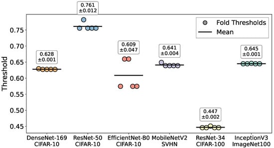
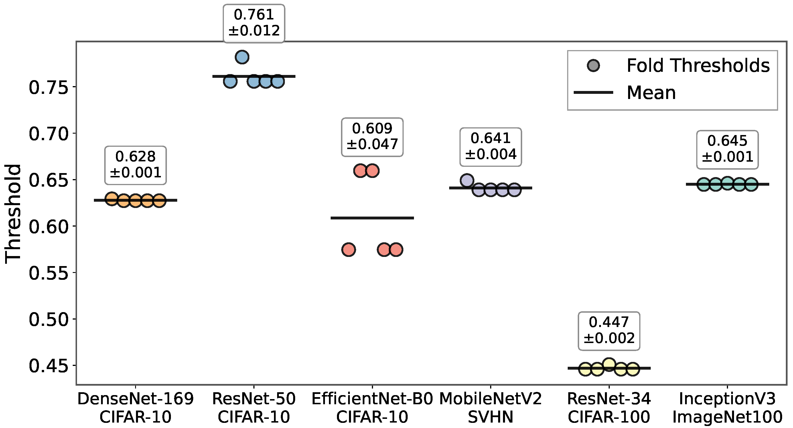
Five out of six models have threshold standard deviations below 0.012, as shown in Figure 6. This means that the threshold selection is very stable. DenseNet-169, MobileNetV2, ResNet-34, and InceptionV3 all have very small threshold deviations (between ±0.001 and ±0.004). This suggests that the best thresholds stay the same across different data partitions. EfficientNet-B0 has a slightly higher threshold deviation (±0.047), but it is still within an acceptable range.

Figure 6. Threshold stability across six source models using 5-fold cross-validation. Error bars indicate standard deviation.

These experimental results demonstrate the robustness and practicality of ProbeSpec. They also show that the fingerprint feature space that ProbeSpec extracts clearly separates stolen models from independent models, rather than being tied to a specific model pool. The stability of optimal thresholds across different data partitions confirms that all models maintain robust performance throughout the cross-validation process, thereby validating the feasibility of deploying ProbeSpec in real-world applications.

4.6. Preliminary Cross-Domain Validation

To initially evaluate the generalization ability of ProbeSpec, we conducted a simple text classification proof-of-concept experiment based on the TinyBERT [27] and GoEmotions [60] dataset (containing 58,000 comments covering 28 sentiment categories).

4.6.1. Cross-Domain Experimental Setup

We applied the three probe types of ProbeSpec to the text domain, with the following setup:

Type A probes used sentiment template sentences with different lexical expressions (e.g., “I have emotion feelings about this”);

Type B probes selected test samples with prediction confidence in the range [0.4, 0.8];

Type C probes connect sentence pairs originating from different sentiment categories. Perturbation is applied at the lexical level via synonym substitution, with substitution probabilities $p\in \{0,0.05,0.1,0.15,0.2\}$. The model pool comprises a total of 78 models.

Model pool composition: 50 stolen models (10 fine-tuned models, 10 pruned models, 10 distillation models, 10 extraction models, and 10 transfer learning models) and 28 independent models (including 10 models trained with different learning rates, 10 models trained on partial data, and 8 models with different architectures).

4.6.2. Results and Discussion

As shown in Table 9, ProbeSpec achieves an overall accuracy of 93.6% (ROC-AUC = 0.972) on TinyBERT models, successfully detecting 96% of stolen models while maintaining a true negative rate of 89.3%. The method achieves 100% detection rate for distillation, extraction, and transfer learning attacks, with only a small number of false negatives in pruned and fine-tuned models. Notably, it perfectly distinguishes models with different architectures, while the main challenge lies in identifying independently trained models with the same architecture and overlapping training data.

Table 9. ProbeSpec performance on TinyBERT-GoEmotions text classification (78 models total).

Category	Count	Detection (%)
Fine-tuning	10	90.0
Pruning	10	90.0
Distillation	10	100.0
Extraction	10	100.0
Transfer	10	100.0
Unrelated	28	89.3
Overall Accuracy	78	93.6
ROC-AUC	-	0.972

Compared to visual tasks (95%+), the performance on text tasks is slightly lower, due to the discrete nature of text and its reduced sensitivity to word-level perturbations. This preliminary result suggests that the core principle of ProbeSpec—multi-probe combined with dynamic perturbation response analysis—can be further extended to copyright protection research in other modalities.

5. Conclusions

Through the above experiments, we have validated the core hypothesis of ProbeSpec: by leveraging multi-dimensional probes, dynamic perturbations, and diverse fingerprint extraction and processing techniques, ProbeSpec can successfully identify stolen models subjected to various attacks, including pruning, fine-tuning, and multiple black-box attacks. ProbeSpec captures behavioral trajectories through its perturbation mechanism and employs three complementary probe types, providing multi-scale coverage of model behavior ranging from low-level frequency sensitivity to high-level semantic relationships. ProbeSpec achieves high identification accuracy while maintaining an extremely low false positive rate, successfully distinguishing independently trained models with identical architectures, thereby ensuring robustness. Furthermore, threshold analysis demonstrates the generalization capability of ProbeSpec’s decision criteria. To verify the generalization ability of our method, we initially validated the cross-domain experiment of TinyBERT-GoEmotions text classification (Section 4.6) and achieved good results. However, the main challenge for text models lies in how to make the probe generation adapt to the discrete lexical space, because the sensitivity of synonym-based perturbations is lower than that of continuous pixel space noise. For future work the following should be explored: (1) systematically extend ProbeSpec to multimodal models; (2) explore probe design for graph neural networks and other non-Euclidean architectures; and (3) combine ProbeSpec with watermarking technology to provide a comprehensive protection framework.

References

- Yuan, C.; Guo, Q.; Zhou, Z.; Fu, Z.; Xia, Z. Deepfake fingerprint detection model intellectual property protection via ridge texture enhancement. IEEE Signal Process. Lett. 2023, 30, 843–847. [Google Scholar] [CrossRef] [Scilit]
- Ahmed, I.; Jeon, G.; Piccialli, F. From artificial intelligence to explainable artificial intelligence in industry 4.0: A survey on what, how, and where. IEEE Trans. Ind. Inform. 2022, 18, 5031–5042. [Google Scholar] [CrossRef] [Scilit]
- Zhou, S.K.; Greenspan, H.; Davatzikos, C.; Duncan, J.S.; Van Ginneken, B.; Madabhushi, A.; Prince, J.L.; Rueckert, D.; Summers, R.M. A review of deep learning in medical imaging: Imaging traits, technology trends, case studies with progress highlights, and future promises. Proc. IEEE 2021, 109, 820–838. [Google Scholar] [CrossRef] [Scilit] [PubMed]
- Howard, J.; Ruder, S. Universal language model fine-tuning for text classification. arXiv 2018, arXiv:1801.06146. [Google Scholar] [CrossRef] [Scilit]
- Shu, H.; Zhu, H. Sensitivity analysis of deep neural networks. In Proceedings of the AAAI Conference on Artificial Intelligence, Honolulu, HI, USA, 27 January–1 February 2019; pp. 4943–4950. [Google Scholar]
- Zhu, M.; Gupta, S. To prune, or not to prune: Exploring the efficacy of pruning for model compression. arXiv 2017, arXiv:1710.01878. [Google Scholar] [CrossRef] [Scilit]
- Hinton, G.; Vinyals, O.; Dean, J. Distilling the knowledge in a neural network. arXiv 2015, arXiv:1503.02531. [Google Scholar] [CrossRef] [Scilit]
- Zagoruyko, S.; Komodakis, N. Paying more attention to attention: Improving the performance of convolutional neural networks via attention transfer. arXiv 2016, arXiv:1612.03928. [Google Scholar]
- Park, W.; Kim, D.; Lu, Y.; Cho, M. Relational knowledge distillation. In Proceedings of the IEEE/CVF Conference on Computer Vision and Pattern Recognition, Long Beach, CA, USA, 16–20 June 2019; pp. 3967–3976. [Google Scholar]
- Orekondy, T.; Schiele, B.; Fritz, M. Knockoff nets: Stealing functionality of black-box models. In Proceedings of the IEEE/CVF Conference on Computer Vision and Pattern Recognition, Long Beach, CA, USA, 15–20 June 2019; pp. 4954–4963. [Google Scholar]
- Papernot, N.; McDaniel, P.; Goodfellow, I.; Jha, S.; Celik, Z.B.; Swami, A. Practical black-box attacks against machine learning. In Proceedings of the 2017 ACM on Asia Conference on Computer and Communications Security, Abu Dhabi, United Arab Emirates, 2–6 April 2017; pp. 506–519. [Google Scholar]
- Pal, S.; Gupta, Y.; Shukla, A.; Kanade, A.; Shevade, S.; Ganapathy, V. Activethief: Model extraction using active learning and unannotated public data. In Proceedings of the AAAI Conference on Artificial Intelligence, New York, NY, USA, 7–12 February 2020; pp. 865–872. [Google Scholar]
- Donahue, J.; Jia, Y.; Vinyals, O.; Hoffman, J.; Zhang, N.; Tzeng, E.; Darrell, T. Decaf: A deep convolutional activation feature for generic visual recognition. In Proceedings of the International Conference on Machine Learning, Beijing, China, 22–24 June 2014; pp. 647–655. [Google Scholar]
- Yosinski, J.; Clune, J.; Bengio, Y.; Lipson, H. How transferable are features in deep neural networks? Adv. Neural Inf. Process. Syst. 2014, 27, 3320–3328. [Google Scholar]
- Wei, C.; Wang, Y.; Gao, K.; Shao, S.; Li, Y.; Wang, Z.; Qin, Z. Pointncbw: Towards dataset ownership verification for point clouds via negative clean-label backdoor watermark. IEEE Trans. Inf. Forensics Secur. 2024, 20, 191–206. [Google Scholar] [CrossRef] [Scilit]
- Boenisch, F. A systematic review on model watermarking for neural networks. Front. Big Data 2021, 4, 729663. [Google Scholar] [CrossRef] [Scilit]
- Chen, X.; Liu, C.; Li, B.; Lu, K.; Song, D. Targeted backdoor attacks on deep learning systems using data poisoning. arXiv 2017, arXiv:1712.05526. [Google Scholar] [CrossRef] [Scilit]
- Chen, J.; Sun, Y.; Wang, J.; Cheng, P.; Ma, X. DEEPJUDGE: A testing framework for copyright protection of deep learning models. In Proceedings of the 2023 IEEE/ACM 45th International Conference on Software Engineering: Companion Proceedings (ICSE-Companion), Melbourne, Australia, 14–20 May 2023; pp. 64–67. [Google Scholar]
- Tan, J.; Zhong, N.; Guo, Y.; Qian, Z.; Zhang, X. Progress in Deep Neural Network Model Watermarking. J. Univ. Shanghai Sci. Technol. 2024, 46, 225–242. [Google Scholar]
- Shao, S.; Zhu, H.; Li, Y.; Yao, H.; Zhang, T.; Qin, Z. Fit-print: Towards false-claim-resistant model ownership verification via targeted fingerprint. arXiv 2025, arXiv:2501.15509. [Google Scholar]
- Szyller, S.; Atli, B.G.; Marchal, S.; Asokan, N. Dawn: Dynamic adversarial watermarking of neural networks. In Proceedings of the 29th ACM International Conference on Multimedia, Virtual, 20–24 October 2021; pp. 4417–4425. [Google Scholar]
- Jiang, Y.; Gao, Y.; Zhou, C.; Hu, H.; Chen, S.; Fu, A.; Susilo, W. Intellectual property protection for deep learning model and dataset intelligence. Eng. Appl. Artif. Intell. 2026, 163, 113024. [Google Scholar] [CrossRef] [Scilit]
- Wang, H.; Wu, X.; Huang, Z.; Xing, E.P. High-frequency component helps explain the generalization of convolutional neural networks. In Proceedings of the IEEE/CVF Conference on Computer Vision and Pattern Recognition, Seattle, WA, USA, 14–19 June 2020; pp. 8684–8694. [Google Scholar]
- Geirhos, R.; Rubisch, P.; Michaelis, C.; Bethge, M.; Wichmann, F.A.; Brendel, W. ImageNet-trained CNNs are biased towards texture; increasing shape bias improves accuracy and robustness. In Proceedings of the International Conference on Learning Representations, Vancouver, BC, Canada, 30 April–3 May 2018. [Google Scholar]
- Garipov, T.; Izmailov, P.; Podoprikhin, D.; Vetrov, D.P.; Wilson, A.G. Loss surfaces, mode connectivity, and fast ensembling of dnns. In Proceedings of the Advances in Neural Information Processing Systems 31, Montréal, QC, Canada, 3–8 December 2018; pp. 8803–8812. [Google Scholar]
- Zhang, H.; Cisse, M.; Dauphin, Y.N.; Lopez-Paz, D. mixup: Beyond empirical risk minimization. arXiv 2017, arXiv:1710.09412. [Google Scholar]
- Jiao, X.; Yin, Y.; Shang, L.; Jiang, X.; Chen, X.; Li, L.; Wang, F.; Liu, Q. Tinybert: Distilling bert for natural language understanding. In Proceedings of the Findings of the Association for Computational Linguistics: EMNLP 2020, Online Event, 16–20 November 2020; pp. 4163–4174. [Google Scholar]
- Lukas, N.; Zhang, Y.; Kerschbaum, F. Deep neural network fingerprinting by conferrable adversarial examples. arXiv 2019, arXiv:1912.00888. [Google Scholar]
- Jia, X.; Wei, X.; Cao, X.; Han, X. Adv-watermark: A novel watermark perturbation for adversarial examples. In Proceedings of the 28th ACM International Conference on Multimedia, Virtual, 12–16 October 2020; pp. 1579–1587. [Google Scholar]
- Hossain, M.S.; Rahman, M.H.; Rahman, M.S.; Hosen, A.S.; Seo, C.; Cho, G.H. Intellectual property theft protection in IoT based precision agriculture using SDN. Electronics 2021, 10, 1987. [Google Scholar] [CrossRef] [Scilit]
- Wang, X.; Lu, Y.; Yan, X.; Yu, L. Wet paper coding-based deep neural network watermarking. Sensors 2022, 22, 3489. [Google Scholar] [CrossRef] [Scilit]
- Tan, J.; Zhong, N.; Qian, Z.; Zhang, X.; Li, S. Deep neural network watermarking against model extraction attack. In Proceedings of the 31st ACM International Conference on Multimedia, Ottawa, ON, Canada, 29 October–3 November 2023; pp. 1588–1597. [Google Scholar]
- Luo, H.; Li, L.; Zhang, X. Secure Neural Network Watermarking Protocol Against Evidence Exposure Attack. IEEE Trans. Multimed. 2025, 27, 5563–5574. [Google Scholar] [CrossRef] [Scilit]
- Ye, Z.; Zhang, X.; Feng, G. Deep neural networks watermark via universal deep hiding and metric learning. Neural Comput. Appl. 2024, 36, 7421–7438. [Google Scholar] [CrossRef] [Scilit]
- Mo, M.; Wang, C.; Guo, Q.; Bian, S.; Huang, Q.; Zhang, X. A novel robust black-box fingerprinting scheme for deep classification neural networks. Expert Syst. Appl. 2024, 252, 124201. [Google Scholar] [CrossRef] [Scilit]
- Adorante, R.; Facchinetti, T.; Pau, D.P. Optimized FreeMark Post-Training White-Box Watermarking of Tiny Neural Networks. Electronics 2025, 14, 4237. [Google Scholar] [CrossRef] [Scilit]
- Jia, H.; Chen, H.; Guan, J.; Shamsabadi, A.S.; Papernot, N. A zest of lime: Towards architecture-independent model distances. In Proceedings of the International Conference on Learning Representations, Vienna, Austria, 4 May 2021. [Google Scholar]
- Cao, X.; Jia, J.; Gong, N.Z. IPGuard: Protecting intellectual property of deep neural networks via fingerprinting the classification boundary. In Proceedings of the 2021 ACM Asia Conference on Computer and Communications Security, Virtual, 7–11 June 2021; pp. 14–25. [Google Scholar]
- Wang, Z.; Wu, D.; Wang, J.; Zhang, X.; Tang, Z. UAPFinger: One-to-many Deep Neural Network Fingerprinting via Universal Adversarial Perturbations. Expert Syst. Appl. 2025, 299, 130048. [Google Scholar] [CrossRef] [Scilit]
- Zhang, G.; Jia, L.; Li, M.; Cai, M. A Fingerprint Scheme for Deep Neural Network Models Based on Adversarial Samples. In Proceedings of the 2024 9th International Conference on Cyber Security and Information Engineering, Kuala Lumpur, Malaysia, 15–17 September 2024; pp. 58–66. [Google Scholar]
- Park, S.; Abuadbba, A.; Wang, S.; Moore, K.; Gao, Y.; Kim, H.; Nepal, S. Deeptaster: Adversarial perturbation-based fingerprinting to identify proprietary dataset use in deep neural networks. In Proceedings of the 39th Annual Computer Security Applications Conference, Austin, TX, USA, 4–8 December 2023; pp. 535–549. [Google Scholar]
- Xu, T.; Wang, C.; Liu, G.; Yang, Y.; Peng, K.; Liu, W. United We Stand, Divided We Fall: Fingerprinting Deep Neural Networks via Adversarial Trajectories. Adv. Neural Inf. Process. Syst. 2024, 37, 69299–69328. [Google Scholar]
- Zhou, Y.; Ni, T.; Lee, W.B.; Zhao, Q. A survey on backdoor threats in large language models (llms): Attacks, defenses, and evaluations. arXiv 2025, arXiv:2502.05224. [Google Scholar] [CrossRef] [Scilit]
- Jaffal, N.O.; Alkhanafseh, M.; Mohaisen, D. Large language models in cybersecurity: A survey of applications, vulnerabilities, and defense techniques. AI 2025, 6, 216. [Google Scholar] [CrossRef] [Scilit]
- Xu, J.; Wang, F.; Ma, M.; Koh, P.W.; Xiao, C.; Chen, M. Instructional fingerprinting of large language models. In Proceedings of the 2024 Conference of the North American Chapter of the Association for Computational Linguistics: Human Language Technologies, (Volume 1: Long Papers), Mexico City, Mexico, 16–21 June 2024; Association for Computational Linguistics: Stroudsburg, PA, USA, 2024; pp. 3277–3306. [Google Scholar]
- Zhao, S.; Jia, M.; Guo, Z.; Gan, L.; Xu, X.; Wu, X.; Fu, J.; Feng, Y.; Pan, F.; Tuan, L.A. A survey of recent backdoor attacks and defenses in large language models. arXiv 2024, arXiv:2406.06852. [Google Scholar]
- Turner, M.R. Texture discrimination by Gabor functions. Biol. Cybern. 1986, 55, 71–82. [Google Scholar] [CrossRef] [Scilit]
- Wallace, G.K. The JPEG still picture compression standard. Commun. ACM 1991, 34, 30–44. [Google Scholar] [CrossRef] [Scilit]
- Krizhevsky, A.; Hinton, G. Learning Multiple Layers of Features from Tiny Images; Technical Report; University of Toronto: Toronto, ON, Canada, 2009. [Google Scholar]
- Netzer, Y.; Wang, T.; Coates, A.; Bissacco, A.; Wu, B.; Ng, A.Y. Reading digits in natural images with unsupervised feature learning. In Proceedings of the NIPS Workshop on Deep Learning and Unsupervised Feature Learning, Granada, Spain, 12–14 December 2011; Volume 2011, p. 7. [Google Scholar]
- Deng, J.; Dong, W.; Socher, R.; Li, L.J.; Li, K.; Fei-Fei, L. Imagenet: A large-scale hierarchical image database. In Proceedings of the 2009 IEEE Conference on Computer Vision and Pattern Recognition, Miami, FL, USA, 20–25 June 2009; pp. 248–255. [Google Scholar]
- He, K.; Zhang, X.; Ren, S.; Sun, J. Deep residual learning for image recognition. In Proceedings of the IEEE Conference on Computer Vision and Pattern Recognition, Las Vegas, NV, USA, 27–30 June 2016; pp. 770–778. [Google Scholar]
- Huang, G.; Liu, Z.; Van Der Maaten, L.; Weinberger, K.Q. Densely connected convolutional networks. In Proceedings of the IEEE Conference on Computer Vision and Pattern Recognition, Honolulu, HI, USA, 21–26 July 2017; pp. 4700–4708. [Google Scholar]
- Tan, M.; Le, Q. Efficientnet: Rethinking model scaling for convolutional neural networks. In Proceedings of the International Conference on Machine Learning, Long Beach, CA, USA, 9–15 June 2019; pp. 6105–6114. [Google Scholar]
- Sandler, M.; Howard, A.; Zhu, M.; Zhmoginov, A.; Chen, L.C. Mobilenetv2: Inverted residuals and linear bottlenecks. In Proceedings of the IEEE Conference on Computer Vision and Pattern Recognition, Salt Lake City, UT, USA, 18–22 June 2018; pp. 4510–4520. [Google Scholar]
- Szegedy, C.; Vanhoucke, V.; Ioffe, S.; Shlens, J.; Wojna, Z. Rethinking the inception architecture for computer vision. In Proceedings of the IEEE Conference on Computer Vision and Pattern Recognition, Las Vegas, NV, USA, 27–30 June 2016; pp. 2818–2826. [Google Scholar]
- Guan, J.; Liang, J.; He, R. Are you stealing my model? sample correlation for fingerprinting deep neural networks. Adv. Neural Inf. Process. Syst. 2022, 35, 36571–36584. [Google Scholar]
- Guan, J.; Liang, J.; Wang, Y.; He, R. Sample correlation for fingerprinting deep face recognition. Int. J. Comput. Vis. 2025, 133, 1912–1926. [Google Scholar] [CrossRef] [Scilit]
- Pan, X.; Yan, Y.; Zhang, M.; Yang, M. Metav: A meta-verifier approach to task-agnostic model fingerprinting. In Proceedings of the 28th ACM SIGKDD Conference on Knowledge Discovery and Data Mining, Washington, DC, USA, 14–18 August 2022; pp. 1327–1336. [Google Scholar]
- Demszky, D.; Movshovitz-Attias, D.; Ko, J.; Cowen, A.; Nemade, G.; Ravi, S. GoEmotions: A dataset of fine-grained emotions. arXiv 2020, arXiv:2005.00547. [Google Scholar]
Disclaimer/Publisher’s Note: The statements, opinions and data contained in all publications are solely those of the individual author(s) and contributor(s) and not of MDPI and/or the editor(s). MDPI and/or the editor(s) disclaim responsibility for any injury to people or property resulting from any ideas, methods, instructions or products referred to in the content. |
© 2026 by the authors. Licensee MDPI, Basel, Switzerland. This article is an open access article distributed under the terms and conditions of the Creative Commons Attribution (CC BY) license.