Multi-Scale Graph-Decoupling Spatial–Temporal Network for Traffic Flow Forecasting in Complex Urban Environments

Abstract

Accurate traffic flow forecasting is a fundamental component of Intelligent Transportation Systems and proactive urban mobility management. However, the inherent complexity of urban traffic flow, characterized by non-stationary dynamics and multi-scale temporal dependencies, poses significant modeling challenges. Existing spatio-temporal models often struggle to reconcile the discrepancy between static physical road constraints and highly dynamic, state-dependent spatial correlations, while their reliance on fixed temporal receptive fields limits the capacity to disentangle overlapping periodicities and stochastic fluctuations. To bridge these gaps, this study proposes a novel Multi-scale Graph-Decoupling Spatial–temporal Network (MS-GSTN). MS-GSTN leverages a Hierarchical Moving Average decomposition module to recursively partition raw traffic flow signals into constituent patterns across diverse temporal resolutions, ranging from systemic daily trends to high-frequency transients. Subsequently, a Tri-graph Spatio-temporal Fusion module synergistically models scale-specific dependencies by integrating an adaptive temporal graph, a static spatial graph, and a data-driven dynamic spatial graph within a unified architecture. Extensive experiments on four large-scale real-world benchmark datasets demonstrate that MS-GSTN consistently achieves superior forecasting accuracy compared to representative state-of-the-art models. Quantitatively, the proposed framework yields an overall reduction in Mean Absolute Error of up to 6.2% and maintains enhanced stability across multiple forecasting horizons. Visualization analysis further confirms that MS-GSTN effectively identifies scale-dependent spatial couplings, revealing that long-term traffic flow trends propagate through global network connectivity while short-term variations are governed by localized interactions.

1. Introduction

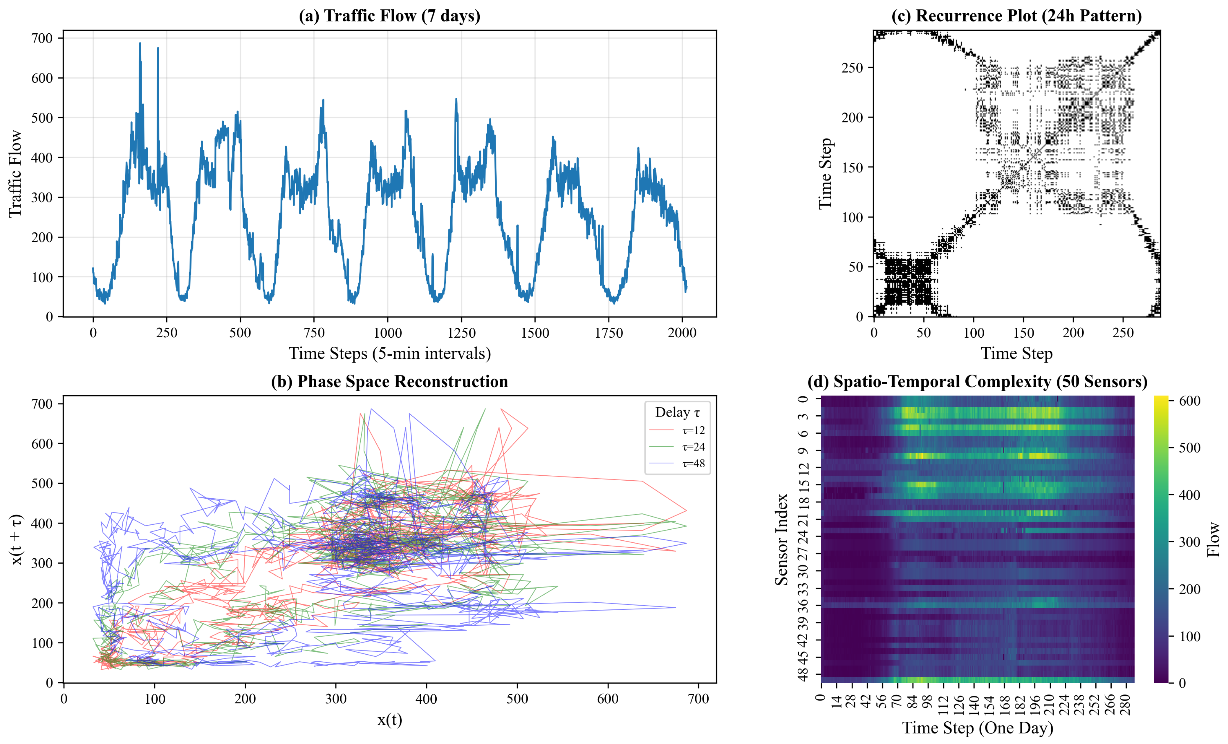
Transportation systems serve as the critical infrastructure of modern smart cities, yet they exhibit intricate spatio-temporal characteristics that pose significant challenges for high-precision forecasting. Within heterogeneous urban road networks, comprising interconnected highways, expressways, and arterial roads, traffic flow evolves through complex mechanisms of stochastic fluctuation, congestion propagation, and feedback loops [1]. As illustrated in Figure 1a, sensor-based measurements reveal multi-scale temporal dependencies, characterized by distinct daily and weekly periodicities intertwined with transient irregularities. These dynamics are further complicated by the non-linear nature of traffic states; the phase space reconstruction in Figure 1b and the recurrence plot in Figure 1c demonstrate that traffic systems often transition between deterministic rhythmic patterns and chaotic states, reflecting the underlying complexity of urban mobility. Spatially, the interaction between distributed monitoring points introduces strong topological correlations, while regional disparities in infrastructure capacity and demand lead to significant spatial non-stationarity, clearly visible in the spatio-temporal heatmaps of multi-sensor arrays (Figure 1d). Moreover, inherent constraints such as sensor noise and uneven detector distribution exacerbate data irregularities [2]. Such combined effects of non-linear evolution and complex network coupling render traditional statistical and shallow learning models inadequate for capturing the full spectrum of traffic dynamics [3]. Therefore, developing a robust forecasting framework that can disentangle high-dimensional spatio-temporal interactions while maintaining computational efficiency remains a pivotal challenge in the field of intelligent transportation systems.

Figure 1. Illustration of complex spatio-temporal characteristics in traffic data: (a) multi-scale temporal patterns with daily and weekly periodicities; (b) phase space reconstruction revealing non-linear dynamics; (c) recurrence plot indicating transitions between regular and chaotic states; (d) spatio-temporal heatmap showing spatial correlations and non-stationarity across sensors.

Driven by the proliferation of high-resolution urban sensing and the evolution of deep representation learning, the focus of traffic analytics has shifted from traditional statistical forecasting to complex spatio-temporal modeling. Given the inherent networked structure of transportation infrastructures, Graph Neural Networks (GNNs) have emerged as a dominant paradigm, owing to their superior capacity to encode non-Euclidean spatial features and leverage the intrinsic topological properties of road networks [4,5]. Unlike conventional grid-based convolutions, GNN-based architectures utilize the physical connectivity of road segments to facilitate message-passing mechanisms, effectively capturing spatial dependencies and the directional propagation of traffic flow [6,7]. However, the spatial interactions in real-world systems are not merely static constraints but are highly dynamic and context-dependent; specifically, the correlation strength between nodes fluctuates significantly according to time-varying traffic volumes and congestion levels [8,9]. Consequently, models restricted to fixed topological maps or static distance-based adjacency matrices often fail to reflect these transient evolutionary characteristics. To bridge this gap, recent advancements have explored adaptive neighbor learning and dynamic graph construction techniques to infer latent dependencies directly from data streams [10,11]. Despite increased flexibility, it remains a formidable challenge to unify stable topological priors with state-dependent dynamic interactions within a single, cohesive framework. Furthermore, existing models frequently overlook the distinct contributions of spatial connections to long-term systemic trends versus short-term stochastic fluctuations [12,13], leading to a fragmented understanding of inter-temporal interaction patterns. Therefore, developing a unified architecture that integrates static structural topology with dynamic, multi-scale spatial relationships is essential for advancing the robustness of traffic forecasting systems.

In parallel with spatial modeling, researchers are increasingly prioritizing the multi-scale temporal structures inherent in traffic sequences [14,15]. Traffic time series are typically characterized by a superposition of long-term evolutionary trends, cyclical periodicities, and high-frequency stochastic fluctuations. To disentangle these patterns, one prevalent research trajectory employs explicit frequency-domain analysis, such as Wavelet and Fourier transforms, combined with seasonal-trend decomposition to partition the series into distinct frequency bands [8,16]. Although effective for noise filtering, such heuristic-based decomposition often struggles to preserve fine-grained temporal transients. Alternatively, deep learning approaches have integrated multi-scale modeling through dilated temporal convolutions, multi-head attention mechanisms, or hybrid architectures with varying receptive fields to capture both local irregularities and global dependencies [17,18]. Despite their empirical success, these architectures face two critical limitations. First, most models treat different scales as independent branches, leading to a lack of explicit cross-scale fusion mechanisms and hindering the formation of a cohesive temporal representation [11,19]. Second, existing frameworks predominantly operate on a finite set of discrete scales, which fails to characterize the continuous spectrum of temporal variations and leads to information loss during transition states [20,21]. Consequently, constructing a unified forecasting framework capable of modeling multi-scale dynamics within a continuous-time perspective, while facilitating seamless cross-scale interaction, emerges as a frontier challenge in advancing intelligent transportation systems.

To address the aforementioned challenges, this study proposes a novel Multi-scale Graph-Decoupling Spatial–temporal Network (MS-GSTN), a unified framework designed to synergistically model heterogeneous spatio-temporal dependencies. Diverging from conventional integrated modeling, MS-GSTN introduces a Hierarchical Moving Average (HMA) decomposition module that adaptively decouples raw traffic flow sequences into multiple constituent temporal patterns, specifically distinguishing long-term systemic trends from short-term stochastic fluctuations. For each decoupled pattern, we develop a Tri-graph Spatio-temporal Fusion (TSF) module. This module jointly encodes three distinct relational dimensions: (1) an adaptive temporal graph to capture latent inter-temporal dependencies, (2) a fixed spatial graph to maintain fundamental topological priors, and (3) a data-driven dynamic spatial graph to reflect transient, state-dependent correlations. An attention-based fusion mechanism is subsequently employed to integrate these static and dynamic embeddings into high-order node representations. Finally, lightweight forecasting heads generate multi-step predictions for each scale, which are re-aggregated to produce the global forecast. Extensive evaluations on four PeMS benchmark datasets (PEMS03, PEMS04, PEMS07, and PEMS08) demonstrate that MS-GSTN consistently outperforms state-of-the-art baselines, validating its superior capability in disentangling complex spatio-temporal dynamics for robust traffic flow forecasting. The main contributions of this study are summarized as follows:

(1)

A Unified Multi-scale Spatio-temporal Architecture: We propose MS-GSTN, which bridges the gap between discrete temporal decomposition and unified graph-based spatial modeling to capture the heterogeneous dependencies inherent in urban traffic.

(2)

Adaptive Hierarchical Decomposition: We design a HMA module that adaptively disentangles raw traffic signals into distinct constituent patterns, such as long-term trends and short-term transients. This prevents the interference of multi-scale features and enhances the granularity of temporal modeling.

(3)

Tri-graph Fusion Mechanism: We develop a novel TSF module that synergistically integrates static structural priors (fixed graphs), transient contextual correlations (dynamic graphs), and latent inter-temporal dependencies (adaptive graphs) through an attention-based coupling mechanism.

(4)

Extensive Empirical Validation: We conduct rigorous benchmarking across four real-world datasets. The results demonstrate that the MS-GSTN model outperforms the benchmark models. Compared to the second-best model, MS-GSTN achieves relative mean absolute error reductions of 0.47%, 0.81%, 6.20%, and 3.02% on the PEMS03, PEMS04, PEMS07, and PEMS08 datasets, respectively.

The rest of this study is organized as follows. Section 2 reviews related work on traffic flow forecasting and multi-scale temporal modeling. Section 3 details the proposed MS-GSTN, elaborating on the mechanisms of hierarchical decomposition and tri-graph fusion. Section 4 presents experimental results and analysis. Finally, Section 5 concludes the study and discusses future research directions.

2. Related Work

2.1. Traffic Flow Forecasting

Traffic flow forecasting leverages longitudinal sensor observations to anticipate future network states, providing a critical foundation for proactive traffic management and Intelligent Transportation Systems [22]. Over the past several decades, the field has undergone a significant paradigm shift, evolving from classical statistical models and traditional machine learning to advanced deep representation learning. Early statistical methods, such as ARIMA and its variants, primarily focused on modeling temporal dependencies within individual roadway segments, often neglecting the complex spatial interactions inherent in large-scale networks [23]. With the increasing availability of high-fidelity sensor data, deep learning architectures, particularly Recurrent Neural Networks (RNNs) and Temporal Convolutional Networks (TCNs), have been extensively deployed to capture non-linear temporal dynamics [24]. However, while these models excel at point-wise or sequence-based temporal extraction, they frequently oversimplify spatial processing through local feature engineering or distance-based aggregation [25,26]. Consequently, such approaches remain inadequate for characterizing the complex propagation mechanisms of congestion waves across heterogeneous road segments [27].

The emergence of Graph Neural Networks (GNNs) has revolutionized traffic flow forecasting by providing a robust framework for learning representations within non-Euclidean topologies, such as urban road networks [28]. By facilitating message-passing and information aggregation across graph edges, GNN-based architectures can effectively encode the physical connectivity and spatial dependencies between sensors. Initial GNN-based models typically relied on static adjacency matrices constructed from geographical distances or road connectivity. To enhance flexibility, subsequent research introduced adaptive graph structures that learn neighborhood weights directly from data, thereby capturing latent inter-sensor similarities [18,29]. More recently, dynamic graph approaches have been proposed to adjust spatial relationships in real-time as traffic states fluctuate, often incorporating attention mechanisms to highlight critical spatio-temporal propagation paths [9,30].

Despite these advancements, several critical limitations persist in current spatio-temporal modeling. First, most existing frameworks rely on a homogenized graph representation during inference, failing to distinguish between stable structural priors (e.g., physical road connectivity) and transient, state-dependent interactions (e.g., congestion-induced correlations) [31,32]. Second, current models predominantly focus on capturing short-term spatial dependencies, often overlooking how spatial interaction patterns evolve and transition across different temporal scales [33]. Such a fragmented view leads to a loss of information regarding long-term systemic trends and multi-scale fluctuations. These gaps underscore an urgent need for a unified forecasting framework that can synergistically model multi-scale temporal dependencies, static topological constraints, and dynamic spatial correlations within a cohesive architecture.

2.2. Multi-Scale Temporal Modeling

Traffic sequences exhibit an inherent multi-scale hierarchy, encompassing long-term evolutionary trends, daily and weekly seasonalities, and stochastic transients triggered by anomalous disturbances or sudden demand shifts [34]. To capture these heterogeneous patterns, existing literature has explored multi-scale characterization through two primary lenses: spectral-based decomposition and deep representation learning. One category of research employs classical signal processing tools, such as Fourier transforms, Wavelet analysis, and Empirical Mode Decomposition, to partition raw sequences into distinct frequency bands [35,36]. While these decomposition-based methods enhance interpretability and noise resilience, they often rely on predefined heuristic filters that struggle to adapt to the highly non-linear and non-stationary nature of urban traffic dynamics [37,38].

Alternatively, recent advancements have integrated multi-scale modeling directly into deep learning architectures. Temporal Convolutional Networks with dilated convolutions and varying kernel sizes have been widely adopted to expand the receptive field, enabling the simultaneous capture of local fluctuations and long-range dependencies [25,26]. Furthermore, recurrent architectures equipped with skip connections or temporal attention mechanisms have been introduced to prioritize periodic cycles and long-term systemic effects [39,40]. In the context of spatio-temporal graph modeling, multi-scale temporal blocks are typically constructed by stacking layers with different dilation factors or employing multi-branch architectures to process traffic information at varying resolutions simultaneously [21].

Despite their empirical successes, these deep multi-scale designs face several critical bottlenecks when applied to complex transportation networks. First, the temporal scales in most models are implicitly defined by fixed hyperparameters—such as kernel dimensions or dilation rates—which limits the framework’s flexibility to adapt to the continuous spectrum of temporal variations found in real-world data [41]. Second, cross-scale interactions are often addressed through superficial operations like simple summation or concatenation, lacking an explicit mechanism for selective information exchange and cross-scale fusion [42]. Consequently, the model may focus on dominant global patterns while disregarding subtle yet critical local transients. Perhaps most importantly, temporal modules are frequently developed in isolation from the spatial graph components, failing to account for how specific temporal-scale patterns (e.g., congestion waves) interact with the underlying road topology. These limitations necessitate the development of a unified, data-driven framework that deeply integrates hierarchical temporal decomposition with adaptive spatial graph modeling, a core objective of the proposed MS-GSTN in this study.

3. Methodology

3.1. Problem Definition

The objective of traffic flow forecasting is to infer future traffic states at multiple sensor locations based on historical observations collected from a road network. Let the traffic system contain N sensor stations, denoted as $\mathcal{V}=\{v_1,v_2,\dots ,v_N\}$, where each $v_i$ represents a fixed point detector installed on a road segment. At discrete time step t, the traffic state observed by all sensors is represented as a matrix ${\mathbf{x}}_t\in {\mathbb{R}}^{N\times F}$, where F is the number of measurement channels (for example flow, speed and occupancy), and the ith row ${\mathbf{x}}_t^{(i,:)}$ corresponds to the measurements at sensor $v_i$. Given a historical sequence of length T, denoted as ${\mathbf{X}}_{t-T+1:t}=[{\mathbf{x}}_{t-T+1},{\mathbf{x}}_{t-T+2},\dots ,{\mathbf{x}}_t]\in {\mathbb{R}}^{N\times T\times F}$, the goal is to forecast the traffic states for the next H time steps, ${\widehat{\mathbf{Y}}}_{t+1:t+H}=[{\widehat{\mathbf{x}}}_{t+1},{\widehat{\mathbf{x}}}_{t+2},\dots ,{\widehat{\mathbf{x}}}_{t+H}]\in {\mathbb{R}}^{N\times H\times F}$.

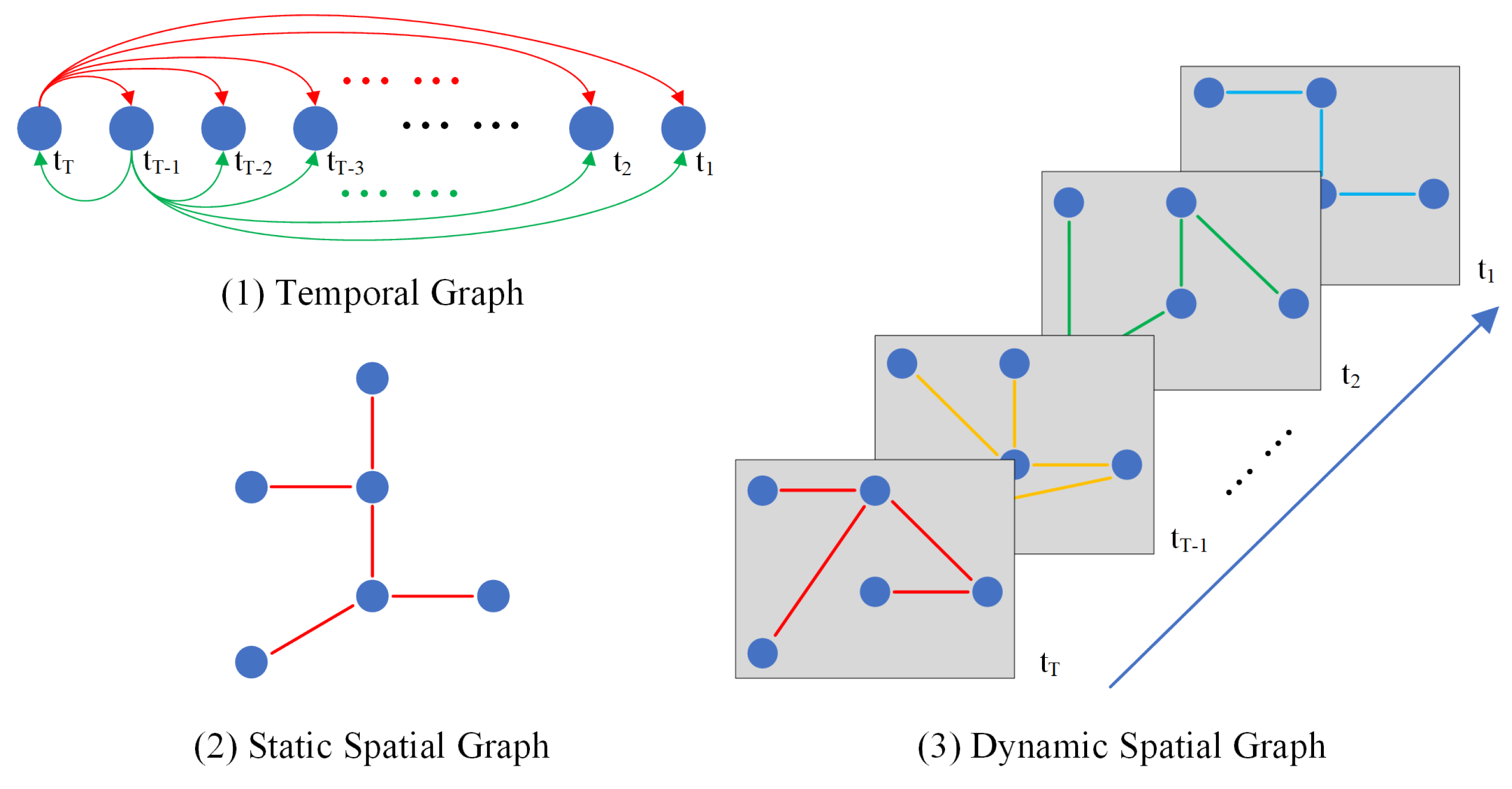
To characterize the heterogeneous spatio-temporal dependencies inherent in the traffic system, this study incorporates three complementary graph structures (Figure 2), namely a temporal graph, a static spatial graph and a dynamic spatial graph. Specific definitions are as follows:

(1)

Temporal graph ${\mathcal{G}}^{\mathrm{temp}}$. To describe temporal correlations among different time steps in the input sequence, such as sequential dependence, periodicity or temporal similarity, we construct a temporal graph that captures the internal temporal structure of the historical inputs:

$${\mathcal{G}}^{\mathrm{temp}}=(\mathcal{T},{\mathcal{E}}^{\mathrm{temp}}),$$

(1)

where $\mathcal{T}=\{1,2,\dots ,T\}$ denotes the temporal indices of the input sequence and ${\mathcal{E}}^{\mathrm{temp}}$ represents the edge set encoding temporal relationships. The temporal adjacency matrix $A^{\mathrm{temp}}\in {\mathbb{R}}^{T\times T}$ captures these correlations.

(2)

Static spatial graph ${\mathcal{G}}^{\mathrm{sta}}$. To represent fixed topological relationships among sensor locations based on the physical connectivity of the road network, we define a static spatial graph as:

$${\mathcal{G}}^{\mathrm{sta}}=(\mathcal{V},{\mathcal{E}}^{\mathrm{sta}}),$$

(2)

where ${\mathcal{E}}^{\mathrm{sta}}$ contains edges derived from the road network structure. The adjacency matrix $A^{\mathrm{sta}}\in {\mathbb{R}}^{N\times N}$ encodes these fixed spatial relationships.

(3)

Dynamic spatial graph ${\mathcal{G}}_t^{\mathrm{dyn}}$. Spatial dependencies among sensors vary with traffic conditions and time, so we introduce a dynamic spatial graph to capture time-varying spatial correlations:

$${\mathcal{G}}_t^{\mathrm{dyn}}=(\mathcal{V},{\mathcal{E}}_t^{\mathrm{dyn}}),$$

(3)

where ${\mathcal{E}}_t^{\mathrm{dyn}}$ represents edges that reflect dynamic spatial relationships at time t. The corresponding dynamic adjacency matrix $A_t^{\mathrm{dyn}}\in {\mathbb{R}}^{N\times N}$ is inferred from data and characterizes these evolving dependencies.

Figure 2. Illustration of three complementary graph structures.

Figure 2. Illustration of three complementary graph structures.

To this end, the core objective of this study is to construct a unified and expressive predictive framework that leverages multi type graph structures and multi-scale temporal features to accurately infer future traffic states from historical observations. Specifically, we aim to learn a mapping function $\mathcal{F}$ that integrates the historical traffic sequence and the defined graph structures to produce multi step forecasts:

$$\mathcal{F}:\{{\mathbf{X}}_{t-T+1:t},{\mathcal{G}}^{\mathrm{temp}},{\mathcal{G}}^{\mathrm{sta}},{\mathcal{G}}_{t-T+1:t}^{\mathrm{dyn}}\}\to {\widehat{\mathbf{Y}}}_{t+1:t+H}.$$

(4)

3.2. Overall Architecture

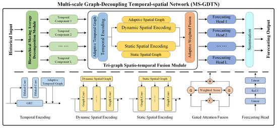
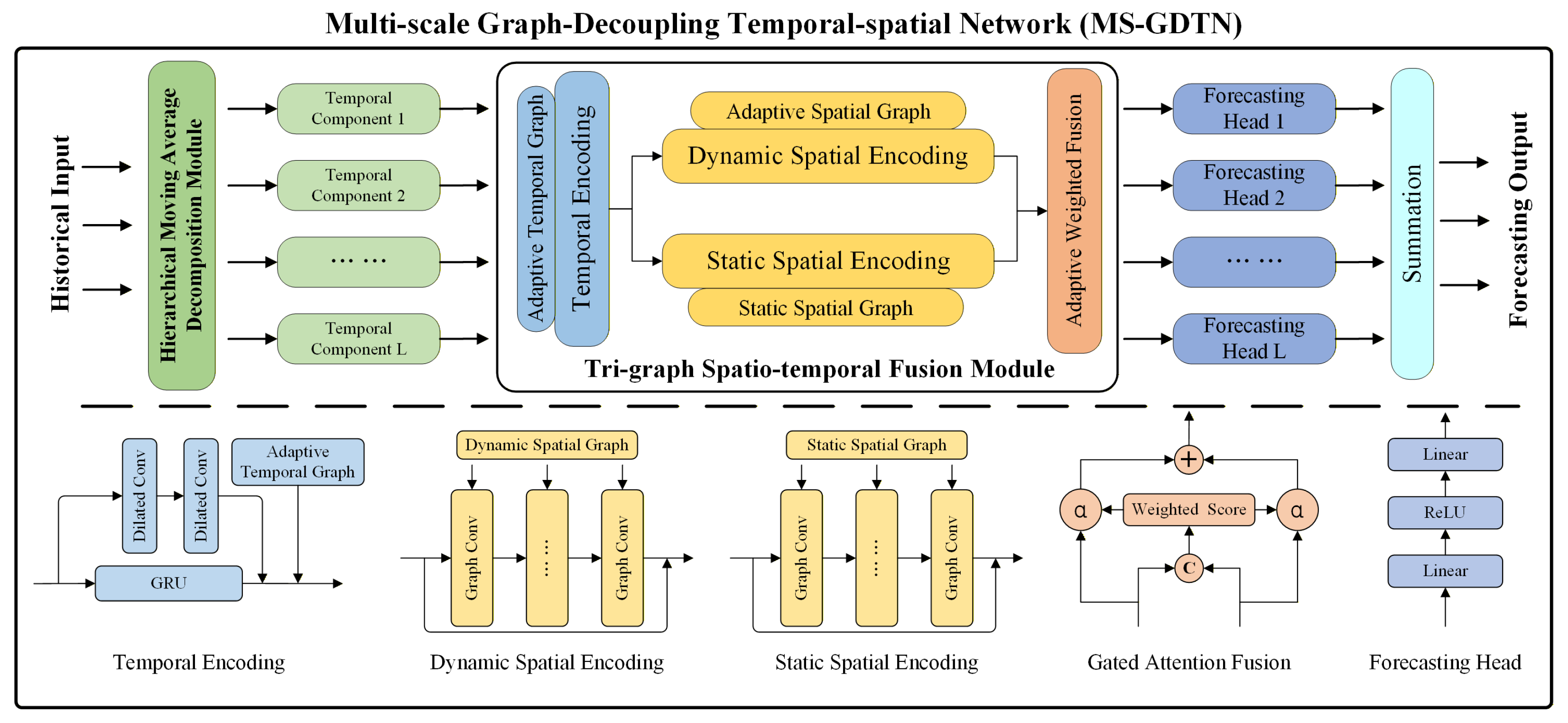
The intricate nature of urban traffic dynamics stems from the superposition of multi-scale temporal variations and deeply coupled spatio-temporal dependencies. To capture these properties within a unified architecture, we propose the Multi-scale Graph-Decoupling Spatial–temporal Network (MS-GSTN). As illustrated in Figure 3, the architecture primarily consists of two pivotal components: the Hierarchical Moving Average (HMA) decomposition module and the Tri-graph Spatio-temporal Fusion (TSF) module.

Figure 3. Architecture of the Multi-scale Graph-Decoupling Spatial–temporal Network.

Given the historical observation tensor ${\mathbf{X}}_{t-T+1:t}\in {\mathbb{R}}^{N\times T\times F}$, where N denotes the number of sensors, T represents the look-back window length, and F signifies the number of feature channels, the HMA module first decomposes the raw signal into K constituent temporal patterns:

$${\left\{{\mathbf{X}}_{t-T+1:t}^{\left(k\right)}\right\}}_{k=1}^K=\mathrm{HMA}\left({\mathbf{X}}_{t-T+1:t}\right),{\mathbf{X}}^{\left(k\right)}\in {\mathbb{R}}^{N\times T\times F},$$

(5)

each pattern k corresponds to a specific temporal resolution, such as long-term systemic trends, low-frequency periodicities, high-frequency stochastic fluctuations, and a residual component.

Subsequently, for each decoupled pattern k, the sub-tensor ${\mathbf{X}}_{t-T+1:t}^{\left(k\right)}$ is processed by the TSF module. This module synergistically exploits three distinct relational dimensions: (i) an adaptive temporal graph ${\mathcal{G}}^{\mathrm{temp},\left(k\right)}$, (ii) a static spatial topology ${\mathcal{G}}^{\mathrm{sta}}$, and (iii) a dynamically inferred spatial graph ${\mathcal{G}}^{\mathrm{dyn},\left(k\right)}$ that reflects transient traffic states at the corresponding scale. The module generates high-order node-level latent representations as follows:

$${\mathbf{H}}^{\left(k\right)}={\Phi }_{\mathrm{TSF}}\left({\mathbf{X}}_{t-T+1:t}^{\left(k\right)},{\mathcal{G}}^{\mathrm{temp},\left(k\right)},{\mathcal{G}}^{\mathrm{sta}},{\mathcal{G}}^{\mathrm{dyn},\left(k\right)}\right)\in {\mathbb{R}}^{N\times D},$$

(6)

where D denotes the hidden embedding dimension. Based on these latent states ${\mathbf{H}}^{\left(k\right)}$, MS-GSTN employs a set of lightweight forecasting heads ${\Psi }^{\left(k\right)}$, specialized for each temporal pattern, to generate multi-step predictions:

$${\widehat{\mathbf{Y}}}_{t+1:t+H}^{\left(k\right)}={\Psi }^{\left(k\right)}\left({\mathbf{H}}^{\left(k\right)}\right)\in {\mathbb{R}}^{N\times H\times F},$$

(7)

where H is the predefined forecasting horizon. To reconstruct the complete signal and produce the final forecast, the outputs from all scale-specific branches are aggregated through a fusion layer (e.g., summation):

$${\widehat{\mathbf{Y}}}_{t+1:t+H}=\sum _{k=1}^K{\widehat{\mathbf{Y}}}_{t+1:t+H}^{\left(k\right)}.$$

(8)

By adopting this “decouple-then-fuse” strategy, MS-GSTN effectively disentangles heterogeneous temporal dynamics, allowing the spatio-temporal fusion engine to focus on scale-specific features. Simultaneously, the joint modeling of static and dynamic graphs ensures that the framework remains robust to both fixed infrastructure constraints and highly volatile, state-dependent spatial correlations.

3.3. Hierarchical Moving Average Decomposition Module

Traffic time series are inherently non-stationary, typically comprising a superposition of long-term evolutionary trends, periodic seasonalities, and high-frequency stochastic fluctuations. To explicitly disentangle these heterogeneous temporal patterns, we develop a Hierarchical Moving Average decomposition module. This module recursively transforms the raw input sequence into a set of constituent patterns across multiple temporal resolutions.

Let $x_i^{\left(f\right)}\left(\tau \right)$ denote the traffic measurement of channel f at sensor $v_i$ and time step $\tau$. For notational clarity, we represent the sequence as $x\left(\tau \right)$ when sensor and channel indices are implicit. Given a historical window ${\left\{x\left(\tau \right)\right\}}_{\tau =t-T+1}^t$, we define the moving average operator ${\mathcal{M}}_w$ with a window size w as follows:

$${\mathcal{M}}_w\left[x\right]\left(\tau \right)={\displaystyle \frac{1}{w}}\sum _{s=0}^{w-1}x(\tau -s),\tau \in \{t-T+1,\dots ,t\},$$

(9)

where zero-padding or boundary replication is applied to maintain sequence length. In this context, larger window sizes act as low-pass filters that emphasize systemic tendencies, while smaller windows retain transient variations.

To implement hierarchical decomposition, we define a decreasing sequence of window sizes $w_1>w_2>\cdots >w_L$, which are calibrated according to the data sampling rate and the temporal scales of interest (e.g., daily or hourly cycles). Starting with the initial sequence $x^{\left(0\right)}\left(\tau \right)=x\left(\tau \right)$, the decomposition proceeds through a successive extraction mechanism:

$$\begin{array}{cccc}\hfill m^{\left(1\right)}\left(\tau \right)& ={\mathcal{M}}_{w_1}\left[x^{\left(0\right)}\right]\left(\tau \right),\hfill & \hfill d^{\left(1\right)}\left(\tau \right)& =x^{\left(0\right)}\left(\tau \right)-m^{\left(1\right)}\left(\tau \right),\hfill \\ \hfill m^{\left(2\right)}\left(\tau \right)& ={\mathcal{M}}_{w_2}\left[d^{\left(1\right)}\right]\left(\tau \right),\hfill & \hfill d^{\left(2\right)}\left(\tau \right)& =d^{\left(1\right)}\left(\tau \right)-m^{\left(2\right)}\left(\tau \right),\hfill \\ \hfill & ⋮\hfill & \hfill & ⋮\hfill \\ \hfill m^{\left(L\right)}\left(\tau \right)& ={\mathcal{M}}_{w_L}\left[d^{(L-1)}\right]\left(\tau \right),\hfill & \hfill d^{\left(L\right)}\left(\tau \right)& =d^{(L-1)}\left(\tau \right)-m^{\left(L\right)}\left(\tau \right),\hfill \end{array}$$

(10)

where $m^{(\ell )}\left(\tau \right)$ represents the extracted smoothed pattern at the ℓ-th scale, and $d^{\left(L\right)}\left(\tau \right)$ denotes the final residual component representing the high-frequency stochastic noise.

By applying these operations independently across all N sensors and F measurement channels, we construct a set of temporal pattern tensors ${\left\{{\mathbf{X}}_{t-T+1:t}^{\left(k\right)}\in {\mathbb{R}}^{N\times T\times F}\right\}}_{k=1}^K$, where $K=L+1$. This set includes the L smoothed components ${\left\{m^{(\ell )}\right\}}_{\ell =1}^L$ and the final residual $d^{\left(L\right)}$. This hierarchical decoupling ensures that the subsequent spatio-temporal fusion module can operate on isolated, scale-specific dynamics, thereby mitigating the interference between heterogeneous temporal features and enhancing the overall robustness of the forecasting system.

3.4. Tri-Graph Spatio-Temporal Fusion Module

The temporal patterns generated by the HMA module retain complex, scale-specific spatio-temporal structures. To effectively capture these multi-scale dependencies, we design a Tri-graph Spatio-temporal Fusion module. For each pattern ${\mathbf{X}}_{t-T+1:t}^{\left(k\right)}\in {\mathbb{R}}^{N\times T\times F}$, the TSF module synergistically integrates three relational perspectives: adaptive temporal dependencies, static physical topology, and dynamic state-aware spatial interactions. The process begins with the construction of an adaptive temporal graph to encode non-local time-axis correlations. These features are then enriched through a hybrid recurrent-convolutional encoder. Subsequently, a dynamic spatial graph is inferred to capture transient interactions, which, alongside the static spatial graph, provides a comprehensive dual-view spatial representation. Finally, an adaptive fusion mechanism yields the high-order latent representation ${\mathbf{H}}^{\left(k\right)}$.

3.4.1. Adaptive Temporal Graph Construction

While traffic observations are sampled at uniform intervals, temporal correlations are often non-linear and non-local due to periodic cycles and stochastic disruptions. To transcend the limitations of sequential modeling, we construct a data-driven temporal graph ${\mathcal{G}}^{\mathrm{temp},\left(k\right)}$ on the time index set $\mathcal{T}=\{1,\dots ,T\}$. For each time step $\tau$, we incorporate a positional encoding ${\mathbf{p}}_{\tau }$, which is transformed via a multi-layer perceptron $g(·)$ to yield latent temporal vectors ${\mathbf{u}}_{\tau }=g\left({\mathbf{p}}_{\tau }\right)$. The pairwise similarity between time steps $\tau$ and ${\tau }^{\prime }$ is defined by their inner product:

$$s_{\tau ,{\tau }^{\prime }}=⟨{\mathbf{u}}_{\tau },{\mathbf{u}}_{{\tau }^{\prime }}⟩.$$

(11)

The resulting similarity scores are normalized via a row-wise softmax to generate the adaptive temporal adjacency matrix ${\mathbf{A}}^{\mathrm{temp}}\in {\mathbb{R}}^{T\times T}$. This mechanism assigns higher weights to temporal positions with similar contextual characteristics (e.g., peak hours across different days), enabling the model to capture long-range periodic dependencies beyond simple Markovian transitions.

3.4.2. Temporal Encoding

For a given pattern k, let ${\mathbf{x}}_i^{\left(k\right)}\in {\mathbb{R}}^{T\times F}$ represent the feature sequence for sensor $v_i$. To capture both causal dynamics and multi-scale receptive fields, we employ a hybrid encoder architecture. First, a Gated Recurrent Unit (GRU) layer captures fine-grained sequential dependencies:

$${\mathbf{H}}_i^{\mathrm{GRU}}=\mathrm{GRU}\left({\mathbf{x}}_i^{\left(k\right)}\right)\in {\mathbb{R}}^{T\times D},$$

(12)

where D is the hidden dimension. Simultaneously, a stack of dilated one-dimensional convolutions is applied to extract broader temporal patterns:

$${\mathbf{H}}_i^{\mathrm{conv}}=\mathrm{DilatedConv}\left({\mathbf{x}}_i^{\left(k\right)}\right)\in {\mathbb{R}}^{T\times D}.$$

(13)

The outputs are integrated via a residual connection to form the initial temporal representation ${\mathbf{H}}_i^{\mathrm{temp}}\in {\mathbb{R}}^{T\times D}$:

$${\mathbf{H}}_i^{\mathrm{temp}}={\mathbf{H}}_i^{\mathrm{GRU}}+{\mathbf{W}}_{\mathrm{res}}{\mathbf{H}}_i^{\mathrm{conv}},$$

(14)

where ${\mathbf{W}}_{\mathrm{res}}\in {\mathbb{R}}^{D\times D}$ is a learnable projection matrix. To further incorporate non-local temporal priors, these embeddings are refined through message passing over the adaptive temporal graph:

$${\overline{\mathbf{H}}}_i^{\mathrm{temp}}={\mathbf{A}}^{\mathrm{temp}}{\mathbf{H}}_i^{\mathrm{temp}}+{\mathbf{H}}_i^{\mathrm{temp}},$$

(15)

where ${\overline{\mathbf{H}}}_i^{\mathrm{temp}}$ denotes the temporally-enhanced embedding for sensor $v_i$.

3.4.3. Dynamic Spatial Graph Construction

Spatial correlations in urban networks are highly volatile and governed by real-time traffic states. While static topology defines the physical constraints, dynamic graphs are essential for modeling congestion propagation. We summarize the temporal evolution of each sensor $v_i$ into a state-aware node embedding ${\mathbf{z}}_i$ using an attentional pooling mechanism:

$${\mathbf{z}}_i=\sum _{\tau =1}^T{\alpha }_{i,\tau }{\overline{\mathbf{h}}}_{i,\tau }^{\mathrm{temp}},{\alpha }_{i,\tau }={\displaystyle \frac{\exp \left(q\left({\overline{\mathbf{h}}}_{i,\tau }^{\mathrm{temp}}\right)\right)}{{\sum }_{{\tau }^{\prime }=1}^T\exp \left(q\left({\overline{\mathbf{h}}}_{i,{\tau }^{\prime }}^{\mathrm{temp}}\right)\right)}},$$

(16)

where $q(·)$ is a learnable scoring function. The dynamic similarity between sensors $v_i$ and $v_j$ is then computed in a learned latent space:

$$s_{ij}^{\mathrm{dyn}}=⟨f\left({\mathbf{z}}_i\right),f\left({\mathbf{z}}_j\right)⟩,$$

(17)

where $f(·)$ is a non-linear transformation. The dynamic spatial adjacency matrix ${\mathbf{A}}^{\mathrm{dyn}}\in {\mathbb{R}}^{N\times N}$ is obtained via row-wise softmax normalization, effectively capturing transient, non-local spatial dependencies.

3.4.4. Dual-View Spatial Encoding and Adaptive Fusion

To exploit both the physical road layout and real-time correlations, we perform parallel graph convolutions on the static graph ${\mathbf{A}}^{\mathrm{sta}}$ and the dynamic graph ${\mathbf{A}}^{\mathrm{dyn}}$. The node features ${\mathbf{u}}_i$ are derived via global temporal pooling: ${\mathbf{u}}_i={\displaystyle \frac{1}{T}}{\sum }_{\tau =1}^T{\overline{\mathbf{h}}}_{i,\tau }^{\mathrm{temp}}$. The spatial embeddings for each view are computed as:

$${\mathbf{h}}_i^{\mathrm{sta}}={\mathrm{GCN}}_{\mathrm{sta}}(\left\{{\mathbf{u}}_j\right\},{\mathbf{A}}^{\mathrm{sta}}),{\mathbf{h}}_i^{\mathrm{dyn}}={\mathrm{GCN}}_{\mathrm{dyn}}(\left\{{\mathbf{u}}_j\right\},{\mathbf{A}}^{\mathrm{dyn}}).$$

(18)

To adaptively balance these complementary views, we utilize a gate-like weighted fusion mechanism. A joint representation ${\mathbf{r}}_i=[{\mathbf{h}}_i^{\mathrm{sta}}\Vert {\mathbf{h}}_i^{\mathrm{dyn}}]$ is projected to compute the fusion weights:

$${[{\alpha }_{i,1},{\alpha }_{i,2}]}^{\top }=\mathrm{softmax}\left({\mathbf{W}}_{\alpha }{\mathbf{r}}_i\right),$$

(19)

where ${\mathbf{W}}_{\alpha }\in {\mathbb{R}}^{2\times 2D}$. The final fused representation for temporal pattern k is given by:

$${\mathbf{h}}_i={\alpha }_{i,1}{\mathbf{h}}_i^{\mathrm{sta}}+{\alpha }_{i,2}{\mathbf{h}}_i^{\mathrm{dyn}}.$$

(20)

Stacking ${\mathbf{h}}_i$ across all sensors yields the final output tensor ${\mathbf{H}}^{\left(k\right)}\in {\mathbb{R}}^{N\times D}$, which is subsequently passed to the multi-step forecasting head.

3.5. Multi-Objective Loss Function

To facilitate the end-to-end training of the proposed MS-GSTN and ensure that each scale-specific branch captures meaningful spatio-temporal dynamics, we define a composite objective function. This strategy involves a global forecasting loss to optimize the final fused output and an auxiliary supervision term designed to refine the individual temporal patterns.

Let $y_{i,h,f}$ denote the ground truth value at sensor $v_i$ for the forecast horizon $h\in \{1,\dots ,H\}$ and feature channel $f\in \{1,\dots ,F\}$, and let ${\widehat{y}}_{i,h,f}$ represent the corresponding element of the aggregated fused forecast ${\widehat{\mathbf{Y}}}_{t+1:t+H}$. The primary objective, ${\mathcal{L}}_{\mathrm{main}}$, utilizes the Mean Absolute Error calculated over all sensors, time horizons, and feature dimensions to ensure robust point-wise accuracy:

$${\mathcal{L}}_{\mathrm{main}}={\displaystyle \frac{1}{F}}\sum _{f=1}^F\left({\displaystyle \frac{1}{NH}}\sum _{i=1}^N\sum _{h=1}^H\left|{\widehat{y}}_{i,h,f}-y_{i,h,f}\right|\right).$$

(21)

In addition to the global loss, we introduce an auxiliary supervision mechanism to prevent the scale-specific branches from converging to trivial solutions or being dominated by a single pattern. For each temporal pattern $k\in \{1,\dots ,K\}$, let ${\widehat{y}}_{i,h,f}^{\left(k\right)}$ be the forecast generated by the k-th specialized forecasting head. We apply a Mean Squared Error auxiliary loss, ${\mathcal{L}}_{\mathrm{aux}}$, to provide stronger gradients for scale-wise feature refinement:

$${\mathcal{L}}_{\mathrm{aux}}={\displaystyle \frac{1}{F}}\sum _{f=1}^F\left({\displaystyle \frac{1}{KNH}}\sum _{k=1}^K\sum _{i=1}^N\sum _{h=1}^H{\left({\widehat{y}}_{i,h,f}^{\left(k\right)}-y_{i,h,f}\right)}^2\right).$$

(22)

By integrating the global optimization objective with localized scale-wise supervision, the total training loss $\mathcal{L}$ is formulated as:

$$\mathcal{L}={\mathcal{L}}_{\mathrm{main}}+{\lambda }_{\mathrm{aux}}{\mathcal{L}}_{\mathrm{aux}},$$

(23)

where ${\lambda }_{\mathrm{aux}}\ge 0$ is a balancing hyperparameter that modulates the influence of the auxiliary supervision. This multi-objective optimization strategy ensures that the model not only achieves superior overall forecasting performance but also effectively disentangles and models the unique evolutionary characteristics of each temporal scale within the unified framework.

4. Experiments

4.1. Datasets

To evaluate the performance of the proposed MS-GSTN, we conduct extensive experiments on four widely-used real-world traffic benchmark datasets: PEMS03, PEMS04, PEMS07, and PEMS08. These datasets are collected by the Caltrans Performance Measurement System (PeMS) and represent various urban road network scales. Each dataset consists of traffic measurements aggregated at 5-min intervals. Following established protocols in the field, we split each dataset into training, validation, and test sets according to a chronological ratio of 6:2:2. All features are scaled to the range $[0, 1]$ using min–max normalization based on the training set statistics to facilitate model convergence. The detailed statistics of these datasets are summarized in Table 1.

Table 1. Statistical summary of the PeMS datasets.

Dataset	Sensors	Time Steps	Interval	Time Range	Features
PEMS03	358	26,208	5 min	1 September 2018–30 November 2018	F
PEMS04	307	16,992	5 min	1 January 2018–28 February 2018	F, S, O
PEMS07	883	28,224	5 min	1 May 2017–31 August 2017	F
PEMS08	170	17,856	5 min	1 July 2016–31 August 2016	F, S, O

Note: F, S, and O denote traffic flow, speed, and occupancy, respectively.

4.2. Experimental Settings

4.2.1. Evaluation Metrics

We employ three standard metrics to quantify the forecasting accuracy: Mean Absolute Error (MAE), Root Mean Squared Error (RMSE), and Mean Absolute Percentage Error (MAPE). In our experimental setup, while the model is trained using normalized data, all evaluations are performed after denormalization to reflect actual deviations. For datasets with multiple channels ($F>1$, such as PEMS04 and PEMS08), we compute the error for each channel independently and report the average performance across all F tasks to ensure mathematical rigor despite different units (e.g., flow, speed, and occupancy). The metrics are defined as follows:

$$\mathrm{MAE}={\displaystyle \frac{1}{F}}\sum _{f=1}^F\left({\displaystyle \frac{1}{NH}}\sum _{i=1}^N\sum _{h=1}^H\left|{\widehat{y}}_{i,h,f}-y_{i,h,f}\right|\right),$$

(24)

$$\mathrm{RMSE}={\displaystyle \frac{1}{F}}\sum _{f=1}^F\sqrt{{\displaystyle \frac{1}{NH}}\sum _{i=1}^N\sum _{h=1}^H{\left({\widehat{y}}_{i,h,f}-y_{i,h,f}\right)}^2},$$

(25)

$$\mathrm{MAPE}={\displaystyle \frac{1}{F}}\sum _{f=1}^F\left({\displaystyle \frac{100\%}{NH}}\sum _{i=1}^N\sum _{h=1}^H\left|{\displaystyle \frac{{\widehat{y}}_{i,h,f}-y_{i,h,f}}{y_{i,h,f}+ϵ}}\right|\right),$$

(26)

where N denote the number of sensors, H the forecasting horizon, and F the number of feature channels. ${\widehat{y}}_{i,h,f}$ and $y_{i,h,f}$ represent the denormalized predicted and ground-truth values, respectively. $ϵ={10}^{-5}$ is a small constant used to avoid division by zero. All metrics are calculated based on the denormalized values on the test set, where lower values signify superior predictive performance.

4.2.2. Implementation Details

MS-GSTN is implemented using PyTorch 2.4.1 and trained on an NVIDIA GeForce RTX 3060 GPU. For all experiments, we set the input window $T=12$ and the forecasting horizon $H=12$, implying that the past one hour of historical data is utilized to predict the traffic state for the subsequent hour. The hidden dimension D is fixed at 64 across all layers. The HMA decomposition module employs a multi-scale window sequence of $[288, 144, 72, 36, 12]$ time steps, which corresponds to physical temporal resolutions of 24 h, 12 h, 6 h, 3 h, and 1 h, respectively. Notably, the HMA decomposition is executed as a data preprocessing step rather than within the training loop. This design choice ensures that the multi-scale signal disentanglement is completed with minimal linear computational overhead, thereby avoiding any significant increase in the model’s overall training complexity or inference latency.

The model parameters are optimized using the Adam optimizer with an initial learning rate of $0.001$. We implement a learning rate decay strategy where the rate is reduced by a factor of 10 if the validation loss fails to improve for five consecutive epochs. To prevent overfitting, early stopping is employed with a patience of 10 epochs, and the maximum number of training epochs is set to 200. The batch size is fixed at 32. For all baseline models, we strictly adhere to the hyperparameter configurations reported in their respective original publications to ensure a fair comparison.

4.3. Baselines

To evaluate the effectiveness of the proposed MS-GSTN, we benchmark it against seven state-of-the-art (SOTA) models that represent diverse technical trajectories in traffic flow forecasting:

• STGCN [43]: Spatio-Temporal Graph Convolutional Network is a pioneering fully convolutional architecture that integrates graph convolutions with 1D temporal convolutions to capture localized spatio-temporal correlations on road networks efficiently.
• DCRNN [44]: Diffusion Convolutional Recurrent Neural Network characterizes traffic dynamics via a diffusion process on a directed graph. It integrates diffusion graph convolutions into a recurrent encoder-decoder framework to capture both spatial and temporal dependencies.
• ASTGCN [45]: Attention-based Spatial–Temporal Graph Convolutional Network employs a spatial–temporal attention mechanism alongside graph and temporal convolutions. It utilizes a three-branch architecture to explicitly model recent, daily, and weekly periodic dependencies.
• STWave [46]: Spatio-Temporal Wavelet Neural Network decomposes traffic sequences into stable trends and stochastic fluctuations using dual-channel spatio-temporal modeling and graph wavelet positional encodings.
• DDGCRNN [47]: Decomposition-based Dynamic Graph Convolutional Recurrent Neural Network generates time-varying adjacency matrices directly from traffic signals. It separates normal and anomalous patterns to jointly learn latent spatial and temporal features.
• STPGNN [4]: Spatio-Temporal Pivotal Graph Neural Network identifies pivotal nodes with extensive topological influence and employs pivotal graph convolutions within a parallel architecture to differentiate between pivotal and non-pivotal node dynamics.
• HSTGNN [6]: Hybrid Spatial–Temporal Graph Neural Network decouples heterogeneous temporal patterns in the frequency domain. It employs a dual-channel temporal learner and hybrid graph learning to capture compound spatial correlations for long-horizon forecasting.

4.4. Performance Comparison and Analysis

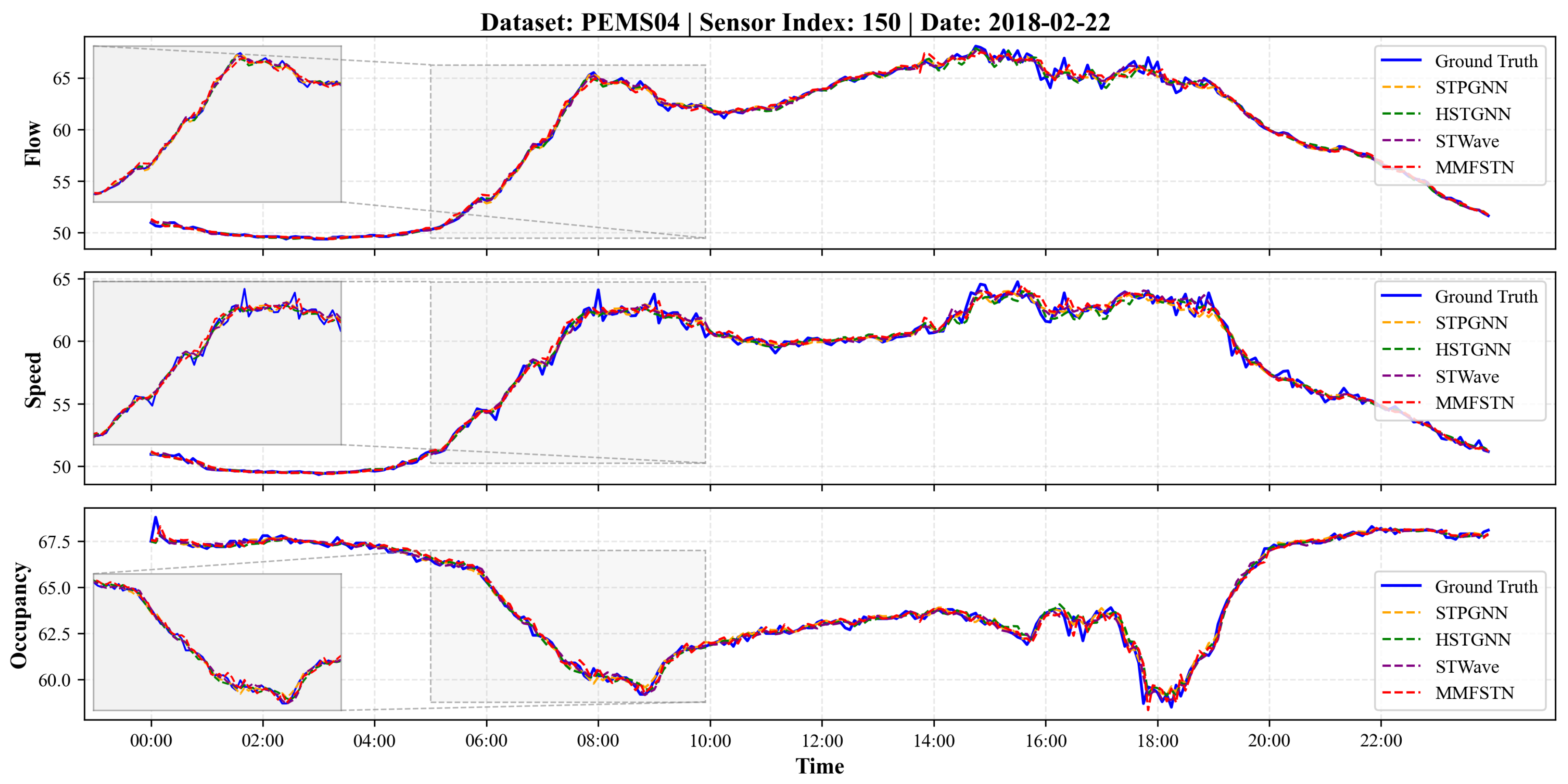
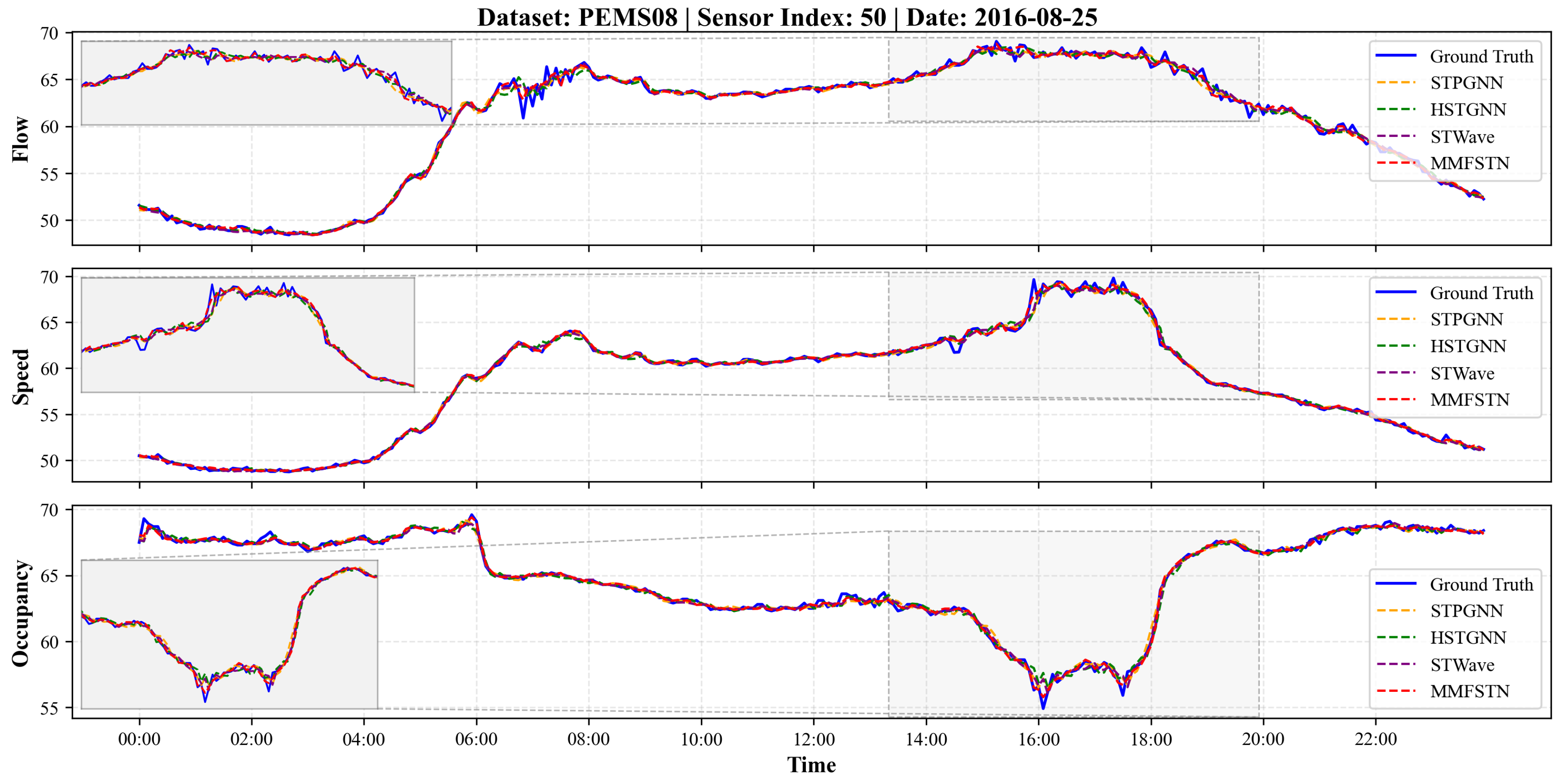
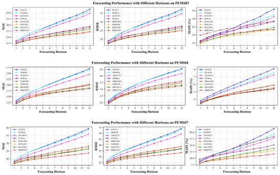
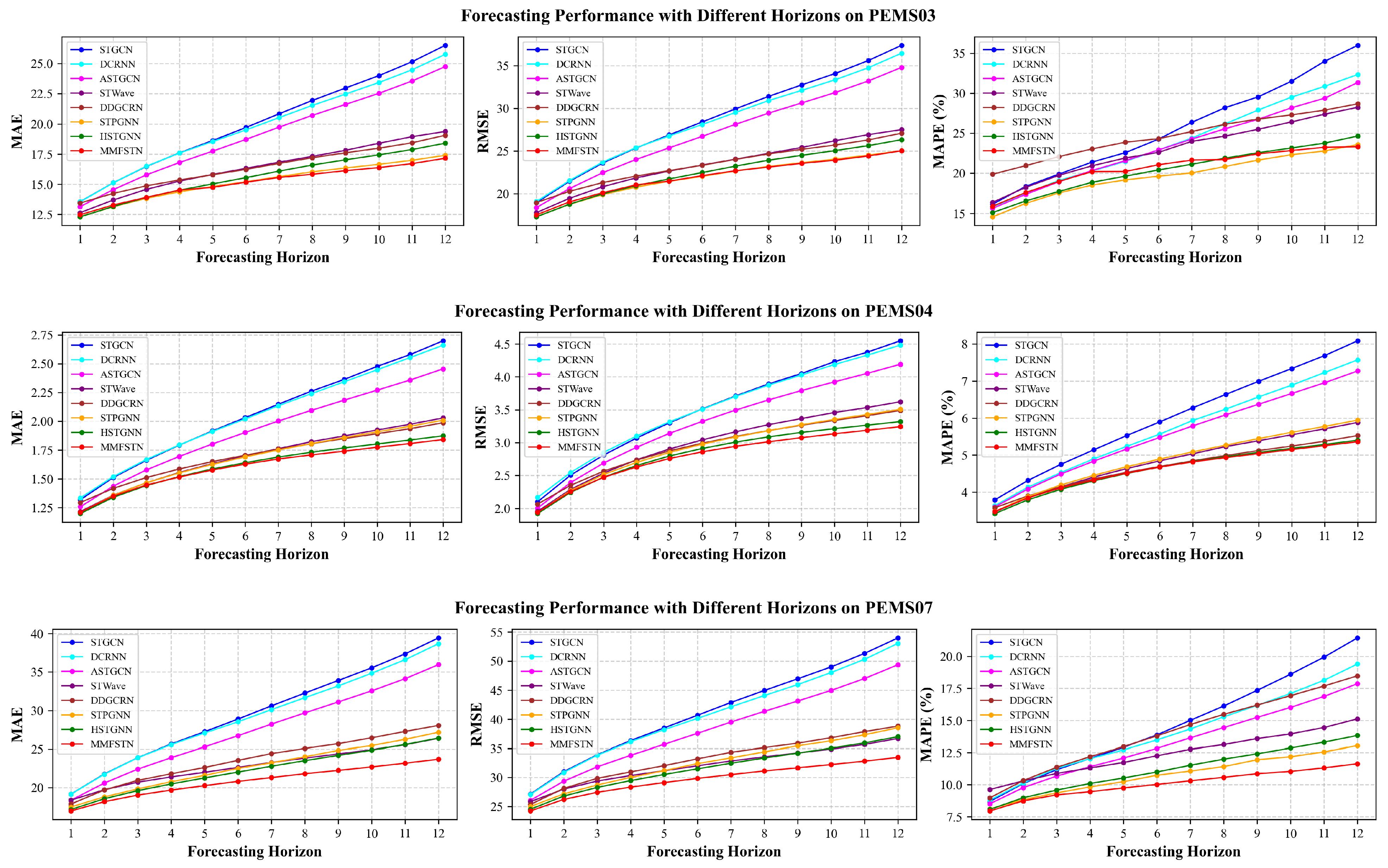
To evaluate the effectiveness of the proposed MS-GSTN, we conduct comprehensive comparisons with several state-of-the-art spatio-temporal models across four benchmark datasets. The forecasting performance in terms of MAE, RMSE, and MAPE is summarized in Table 2. Additionally, Figure 4 provides a visualization of the forecasting results for selected sensors in the PEMS04 and PEMS08 datasets, while Figure 5 illustrates the error evolution across different forecasting horizons.

Table 2. Performance comparison on four PeMS datasets.

Model	PEMS03			PEMS04			PEMS07			PEMS08
	MAE	RMSE	MAPE (%)	MAE	RMSE	MAPE (%)	MAE	RMSE	MAPE (%)	MAE	RMSE	MAPE (%)
STGCN	20.2081	28.8088	25.6858	2.0629	3.5082	6.0386	29.6500	41.3880	14.7683	1.6700	2.7350	4.6530
DCRNN	19.9154	28.4655	24.0252	2.0518	3.5068	5.7042	29.2628	40.8175	14.0681	1.6266	2.6709	4.3146
ASTGCN	19.1362	27.1244	23.5204	1.9191	3.2981	5.5677	27.4207	38.3053	13.2748	1.5302	2.5163	4.2674
STWave	16.4159	23.3861	22.9996	1.6916	2.9896	4.8457	22.7815	32.0574	12.4195	1.3547	2.2704	3.7861
DDGCRN	16.4138	23.4596	24.6777	1.6982	2.9464	4.6935	23.6370	33.2041	14.0833	1.4341	2.4079	3.8291
STPGNN	15.2287	21.9347	19.7428	1.6815	2.9227	4.8942	22.6776	32.4916	10.7717	1.3272	2.2509	3.6768
HSTGNN	15.6575	22.4792	20.4559	1.6179	2.8369	4.6265	22.2204	31.5974	11.1757	1.3210	2.2236	3.6401
MS-GSTN	15.1573	21.9947	20.7656	1.6048	2.7925	4.6271	20.8436	29.7671	10.0672	1.2811	2.2209	3.5921

Note: The best results are highlighted in bold.

Figure 4. Visualization of traffic flow forecasting results on PEMS04 and PEMS08 datasets.

Figure 5. Forecasting performance at different horizons on four datasets.

4.4.1. Overall Comparative Analysis

As shown in Table 2, MS-GSTN outperforms other models across most metrics on all four datasets, demonstrating its exceptional ability to model high-dimensional spatio-temporal dependencies. Compared to the second-best benchmark model, MS-GSTN yields relative MAE reductions of approximately 0.47%, 0.81%, 6.20%, and 3.02% on PEMS03, PEMS04, PEMS07, and PEMS08, respectively. These improvements are especially notable in large-scale and heterogeneous road networks, such as PEMS03 (358 sensors) and PEMS07 (883 sensors). In these scenarios, the spatial correlations are extremely dense and highly non-stationary. Models like STGCN or DCRNN, which rely on fixed adjacency matrices, struggle to balance long-range structural constraints with local propagation. In contrast, MS-GSTN’s TSF module synergistically leverages static topology and dynamic state-aware graphs, allowing it to effectively filter out spatial noise while preserving critical systemic trends.

Furthermore, MS-GSTN achieves the lowest RMSE on PEMS04, PEMS07, and PEMS08, demonstrating its resilience to extreme value deviations. Specifically, during peak-period transitions (e.g., the rapid onset of morning and evening rush hours), traffic flow exhibits high non-stationarity, with frequent sudden changes and sharp spikes. As visualized in the zoomed-in segments of Figure 4, MS-GSTN tracks these abrupt transitions with significantly higher accuracy than benchmark models. Decomposition-based methods, such as STWave, often oversmooth these sudden fluctuations due to fixed filtering. Static-graph models, such as STGCN, tend to underestimate the amplitude of congestion peaks. However, MS-GSTN successfully captures these changes, which is due to the combined effect of the HMA and TSF modules. The HMA module separates these high-frequency transients into specific scales, and the TSF module updates the dynamic spatial graph in real time to reflect the propagation of congestion shocks.

In contrast, during off-peak periods when traffic patterns are relatively stable and governed by deterministic periodicities (e.g., midday or late night), the performance gap between MS-GSTN and other benchmark models narrows. In these steady-state scenarios, the systemic trend component of our model provides a consistent baseline comparable to those of established models. This differentiation shows that MS-GSTN’s core strength lies in its dynamic sensitivity to non-stationary mutations. This allows MS-GSTN to maintain robust accuracy in the most challenging and volatile traffic states while remaining as stable as benchmark models in routine scenarios.

4.4.2. Multi-Horizon Stability

Figure 5 depicts the evolution of MAE, RMSE, and MAPE across 12 forecasting horizons (up to 60 min). Although the forecasting error naturally accumulates over time for all models, the error curves of MS-GSTN remain consistently lower and exhibit a significantly flatter growth trajectory. In contrast to STWave and DDGCRN, MS-GSTN demonstrates superior error control at medium-to-long horizons (e.g., 30–60 min). This stability is attributed to the hierarchical moving average module, which preserves long-term systemic trends while isolating high-frequency noise, thereby preventing small-scale fluctuations from contaminating the long-range prediction signal.

4.4.3. Sensitivity Analysis of Temporal Patterns

To investigate how the number of temporal patterns (K) and specific temporal resolutions influence the forecasting efficacy of MS-GSTN, we evaluated four variants by adjusting the hierarchical window sequence. The results are summarized in Table 3. As shown in Table 3, increasing the granularity of the temporal patterns from M3 to M6 results in consistent performance improvements across all datasets. For example, on the PEMS07 dataset, the mean absolute error (MAE) decreases significantly from 22.48 (M3) to 20.84 (M6), reflecting a 7.3% improvement. These results suggest that a multi-scale hierarchy is essential for reconciling systemic trends and stochastic bursts. Specifically, the transition from M3 to M6 reflects the integration of increasingly broader temporal contexts, spanning from one-hour to 24-h cycles. By incorporating the 288-step (24-h) window, M6 provides a stable global anchor that enables the model to distinguish deterministic daily periodicities from high-frequency stochastic variations. This hierarchical structure enables the subsequent Tri-graph Fusion module to focus on scale-specific spatial dependencies instead of being overwhelmed by the full complexity of the raw signal.

Table 3. Effect of the number of temporal patterns in MS-GSTN on four PeMS datasets.

Model	PEMS03			PEMS04			PEMS07			PEMS08
	MAE	RMSE	MAPE (%)	MAE	RMSE	MAPE (%)	MAE	RMSE	MAPE (%)	MAE	RMSE	MAPE (%)
MS-GSTN (M3)	16.0905	23.2237	21.1301	1.7036	3.0101	4.9087	22.4773	32.1712	11.0567	1.3502	2.3055	3.7411
MS-GSTN (M4)	15.5914	22.4146	20.4205	1.6592	2.8999	4.7849	22.0449	31.5108	10.9899	1.3004	2.1989	3.6022
MS-GSTN (M5)	15.2290	21.8438	19.8531	1.6249	2.8510	4.6871	20.9415	30.0573	10.2351	1.3081	2.2092	3.6231
MS-GSTN (M6)	15.1573	21.9947	20.7656	1.6048	2.7925	4.6271	20.8436	29.7671	10.0672	1.2811	2.2209	3.5921

Note: M3–M6 represent configurations with $K=3$ to $K=6$ temporal patterns. Given the 5-min sampling, the window sequences $[288, 144, 72, 36, 12]$ correspond to physical scales of {24 h, 12 h, 6 h, 3 h, 1 h}. Specifically: M3 = {3 h, 1 h, residual}; M4 = {6 h, 3 h, 1 h, residual}; M5 = {12 h, 6 h, 3 h, 1 h, residual}; M6 = {24 h, 12 h, 6 h, 3 h, 1 h, residual}. The best results are highlighted in bold.

However, we observe that the marginal gains from M5 to M6 are smaller compared to the leap from M3 to M4. This suggests a saturation effect in temporal decoupling. While finer-grained scales improve disentanglement, excessive decomposition can lead to over-parameterization, making it harder to optimize the multi-objective loss function. Nevertheless, the current six-scale configuration (M6) strikes the optimal balance, ensuring that the MS-GSTN remains robust to both long-term evolutionary trends and high-frequency stochastic fluctuations.

4.5. Ablation Study

To quantify the contribution of each core component in MS-GSTN, we evaluate four variants:

• w/o TG: Removes the adaptive temporal graph, relying solely on sequential modeling.
• w/o DG: Removes the dynamic spatial graph, using only static physical topology.
• w/o SG: Removes the static spatial graph, relying exclusively on data-driven correlations.
• w/o HMA: Bypasses the Hierarchical Moving Average decomposition module and feeds the un-decomposed raw traffic sequence directly into the spatio-temporal fusion engine.

The results in Table 4 demonstrate that all components are integral to the model’s performance. Notably, the most substantial degradation occurs in the w/o HMA variant across all datasets. This significant increase in error metrics underscores that the Hierarchical Moving Average module is the cornerstone of MS-GSTN; without it, the model fails to disentangle the multi-scale temporal hierarchy (e.g., long-term trends vs. high-frequency fluctuations), leading to severe feature interference and a diminished capacity to handle non-stationary traffic signals. Furthermore, the performance decline in w/o SG and w/o DG variants justifies our graph-decoupling strategy, proving that neither the fixed physical topology nor the transient state-dependent correlations alone are sufficient for comprehensive spatio-temporal representation. Finally, the w/o TG variant confirms that the adaptive temporal graph provides essential non-local refinement that further elevates forecasting precision. Overall, the ablation study validates the synergistic design of MS-GSTN, where each module plays a critical role in capturing the complex dynamics of urban traffic.

Table 4. Ablation study of MS-GSTN on four PeMS datasets.

Model	PEMS03			PEMS04			PEMS07			PEMS08
	MAE	RMSE	MAPE (%)	MAE	RMSE	MAPE (%)	MAE	RMSE	MAPE (%)	MAE	RMSE	MAPE (%)
w/o TG	15.2899	22.0968	22.8234	1.6155	2.7983	4.6978	20.8515	29.7635	10.6934	1.2990	2.2345	3.6602
w/o DG	15.5314	22.2932	25.5544	1.6394	2.8128	4.8201	20.9577	29.8518	11.7896	1.3340	2.2634	3.7764
w/o SG	15.8232	22.5428	28.3791	1.6691	2.8322	4.9626	21.1090	29.9876	12.8791	1.3749	2.2978	3.9100
w/o HMA	16.2086	22.8894	31.4677	1.7096	2.8603	5.1436	21.3440	30.2106	14.0602	1.4274	2.3436	4.0780
MS-GSTN	15.1573	21.9947	20.7656	1.6048	2.7925	4.6271	20.8436	29.7671	10.0672	1.2811	2.2209	3.5921

Note: TG, DG, SG, and HMA denote the adaptive temporal graph, dynamic spatial graph, static spatial graph, and hierarchical moving average decomposition, respectively. The best results are highlighted in bold.

4.6. Visualization of Hierarchical Patterns and Dynamic Spatial Interactions

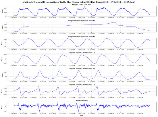
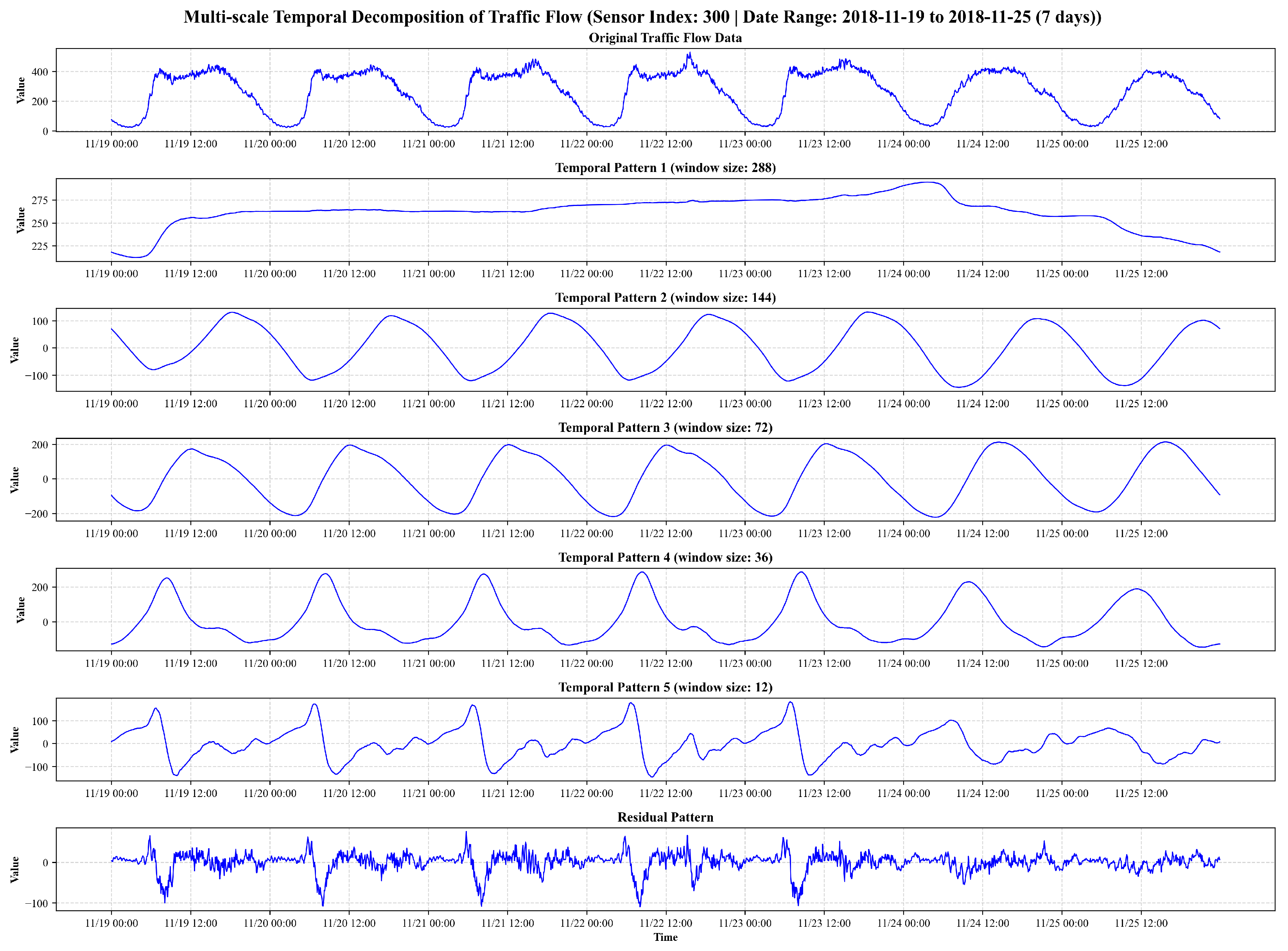
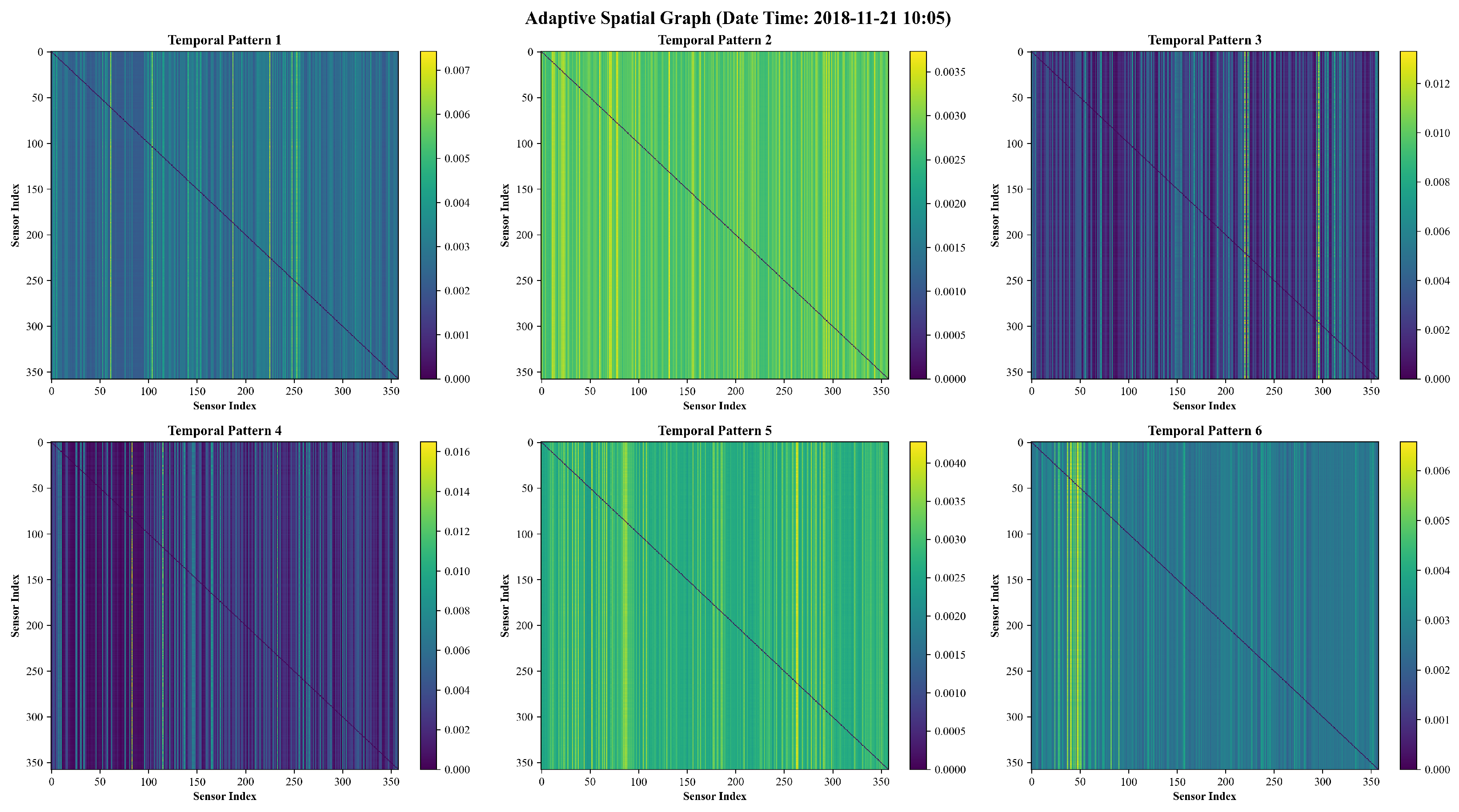
To gain further insight into the internal representations learned by MS-GSTN, we visualize the decomposed temporal components and their corresponding scale-specific dynamic spatial graphs using the PEMS03 dataset, as illustrated in Figure 6 and Figure 7. These visualizations elucidate how the framework leverages the HMA decomposition module to disentangle complex signals into interpretable patterns and associates them with distinct spatial interaction structures within the TSF module.

Figure 6. Visualization of multi-scale temporal patterns on PEMS03 dataset.

Figure 7. Visualization of dynamic spatial graphs on PEMS03 dataset.

4.6.1. Interpretability of HMA Temporal Patterns

Figure 6 presents the hierarchical decomposition of a one-week traffic flow sequence at a representative sensor station. The raw signal in the top panel exhibits a mixture of daily cycles, intra-day peaks, and stochastic fluctuations. Through the HMA module, the signal is partitioned into five constituent patterns, corresponding to window sizes of 288, 144, 72, 36, and 12 steps, and a residual. Given the 5-min sampling interval, these scales align with physical periods of approximately 24 h, 12 h, 6 h, 3 h, and 1 h, respectively.

Specifically, this hierarchical decomposition provides granular insights into the traffic signal by partitioning it into distinct semantic layers. The coarsest scales, represented by Patterns 1 and 2 (24 h and 12 h), successfully capture the slowly varying baseline and macroscopic weekly trends, reflecting the fundamental demand contrast between weekday commute cycles and weekend relaxation while serving as a stable anchor for the overall forecasting range. Building upon this foundation, the intermediate scales in Patterns 3 and 4 (6 h and 3 h) highlight recurrent sub-diurnal dynamics that align precisely with the predictable evolution of morning and evening peak periods, effectively capturing the deterministic acceleration and deceleration phases of urban mobility. Finally, the finest scales, including Pattern 5 and the Residual (1 h and below), isolate the sharpest transitions and high-frequency stochastic noise, such as localized traffic bursts, abrupt mutations during congestion onset, and sensor-level irregularities, that are typically obscured by the high-magnitude baseline in the raw signal.

The hierarchical decoupling of these features effectively mitigates the interference between heterogeneous temporal dynamics, as isolating high-magnitude systemic trends from low-magnitude stochastic transients ensures that the forecasting heads for coarser scales maintain long-term stability without being influenced by high-frequency volatility. Consequently, the specialized branches for fine-grained scales can adaptively model non-linear mutations with higher sensitivity, a multi-resolution approach that prevents error accumulation caused by feature entanglement and ensures high-fidelity predictions during volatile peak-hour transitions while maintaining baseline robustness during stable off-peak periods.

4.6.2. Scale-Dependent Dynamic Spatial Coupling

Figure 7 visualizes the learned dynamic spatial adjacency matrices ${\mathbf{A}}^{\mathrm{dyn}}$ for different temporal components at a fixed time instance. The heatmaps reveal a significant transition in spatial interaction structures as the temporal resolution varies, demonstrating the effectiveness of the graph-decoupling strategy.

For the coarsest components representing long-term systemic trends (Pattern 1), the dynamic graphs are notably dense and homogeneous, as indicated by the widespread lighter colors in the heat map. This pattern reflects broad, network-wide synchronization, in which background traffic loads evolve along similar trajectories, driven by citywide systemic demand. As the resolution shifts to intermediate scales (Patterns 2–4), the spatial weights transition into a more structured form, characterized by prominent vertical stripes. These stripes signify regional synchronization, in which specific, influential transport corridors and functional zones dominate subnetwork dynamics. At the finest scales and residuals, the matrices become significantly sparser and feature localized high-weight clusters. This indicates that high-frequency fluctuations and transient disturbances, such as sudden congestion shockwaves, are governed by immediate neighborhood interactions rather than global network states.

This visual evidence strongly validates the graph-decoupling strategy of MS-GSTN, demonstrating that traffic spatial dependencies are scale-dependent by nature. Long-term trends require a dense representation to capture systemic evolution, while high-frequency transients demand a sparse, focused graph to model localized propagation. MS-GSTN effectively reconciles the discrepancy between global network connectivity and state-dependent local interactions by learning these distinct topologies simultaneously. This multi-scale spatial modeling approach outperforms traditional static-graph methods in complex, non-stationary urban environments.

5. Conclusions

Urban transportation systems serve as the essential backbone of modern smart cities, yet their inherent complexity, characterized by non-linear dynamics, multi-scale temporal dependencies, and high-dimensional spatial correlations, presents a formidable challenge for accurate traffic flow forecasting. This study addresses these challenges by proposing a novel Multi-scale Graph-Decoupling Spatial–temporal Network (MS-GSTN), a unified framework designed to disentangle and model the heterogeneous evolution of traffic flows. By integrating a Hierarchical Moving Average decomposition module with a Tri-graph Spatio-temporal Fusion module, the proposed MS-GSTN effectively bridges the gap between discrete signal decomposition and continuous spatio-temporal representation learning.

The empirical results across four large-scale benchmark datasets (PEMS03, PEMS04, PEMS07, and PEMS08) demonstrate that MS-GSTN consistently outperforms state-of-the-art baselines. The success of the model can be attributed to its unique “decouple-then-fuse” strategy: the HMA module mitigates the impact of non-stationary noise by isolating systemic trends from stochastic fluctuations, while the TSF module adaptively captures scale-dependent spatial interactions. Notably, our analysis reveals a critical insight into urban mobility patterns: long-term systemic trends exhibit broad, network-wide correlations governed by fixed topological constraints, whereas short-term transients are dominated by localized, state-dependent couplings. The robust performance of MS-GSTN, particularly its stability over long-term forecasting horizons and its fidelity during peak-period transitions, underscores its potential as a reliable tool for real-world Intelligent Transportation Systems.

Despite the advancements achieved, this study opens several avenues for future research. First, we aim to extend the evaluation of MS-GSTN to more recent and geographically diverse urban datasets to further verify its cross-city generalization and robustness in evolving transportation environments. Second, while MS-GSTN excels in modeling intrinsic traffic dynamics, the integration of exogenous environmental variables—such as extreme weather events, social activities, and point-of-interest distributions—could further enhance the model’s predictive resilience under anomalous conditions. Third, we plan to explore more computationally efficient graph convolution kernels or sparse attention mechanisms to ensure the framework’s scalability for real-time deployment in city-wide sensor networks. Finally, extending the current deterministic forecasting approach toward probabilistic modeling will be essential for quantifying prediction uncertainty, thereby providing more informed decision support for urban traffic management and autonomous navigation systems.

References

- Liu, X.; Qin, L.; Xu, M.; Zhou, Y.; Wang, B.; Yu, W.; Xiong, W. A comprehensive review of traffic flow forecasting based on deep learning. Neurocomputing 2025, 668, 132269. [Google Scholar] [CrossRef] [Scilit]
- Jiang, W.; Luo, J. Graph neural network for traffic forecasting: A survey. Expert Syst. Appl. 2022, 207, 117921. [Google Scholar] [CrossRef] [Scilit]
- Zhang, Y.; Zhang, Y.; Haghani, A. A hybrid short-term traffic flow forecasting method based on spectral analysis and statistical volatility model. Transp. Res. Part C Emerg. Technol. 2014, 43, 65–78. [Google Scholar] [CrossRef] [Scilit]
- Kong, W.; Guo, Z.; Liu, Y. Spatio-Temporal Pivotal Graph Neural Networks for Traffic Flow Forecasting. Proc. AAAI Conf. Artif. Intell. 2024, 38, 8627–8635. [Google Scholar] [CrossRef] [Scilit]
- Li, M.; Zhu, Z. Spatial-Temporal Fusion Graph Neural Networks for Traffic Flow Forecasting. Proc. AAAI Conf. Artif. Intell. 2021, 35, 4189–4196. [Google Scholar] [CrossRef] [Scilit]
- Wang, P.; Feng, L.; Zhu, Y.; Wu, H. Hybrid spatial-temporal graph neural network for traffic forecasting. Inf. Fusion 2025, 118, 102978. [Google Scholar] [CrossRef] [Scilit]
- Liu, W.; Li, H.; Zhang, H.; Xue, J.; Sun, S. Dynamic Spatio-Temporal Graph Fusion Network modeling for urban metro ridership prediction. Inf. Fusion 2025, 117, 102845. [Google Scholar] [CrossRef] [Scilit]
- Xu, J.; Yang, J.; Huang, Y.; Por, L.Y.; Chen, X.; Zhao, C. DFGNet: A dual-pathway graph neural network via frequency decomposition for spatiotemporal forecasting. Expert Syst. Appl. 2026, 297, 129518. [Google Scholar] [CrossRef] [Scilit]
- Wang, P.; Feng, L.; Zhang, W.; Hui, K. TWIST: An Efficient Spatial—Temporal Transformer With Temporal Window and Sparse Attention for Traffic Forecasting. IEEE Internet Things J. 2025, 12, 26799–26815. [Google Scholar] [CrossRef] [Scilit]
- Jiang, J.; Han, C.; Zhao, W.X.; Wang, J. PDFormer: Propagation Delay-Aware Dynamic Long-Range Transformer for Traffic Flow Prediction. Proc. AAAI Conf. Artif. Intell. 2023, 37, 4365–4373. [Google Scholar] [CrossRef] [Scilit]
- Wang, C.; Li, Z.; Yu, J.; Xu, L. High-low frequency dynamic interactive fusion network for multivariate time series forecasting. Knowl.-Based Syst. 2025, 310, 112951. [Google Scholar] [CrossRef] [Scilit]
- Ren, Q.; Li, Y.; Liu, Y. Transformer-enhanced periodic temporal convolution network for long short-term traffic flow forecasting. Expert Syst. Appl. 2023, 227, 120203. [Google Scholar] [CrossRef] [Scilit]
- Chiang, H.S.; Lin, K.H.; Lin, H.; Chen, M.Y. Short-term traffic flow prediction based on deep learning approach with inter-day and intra-day strategies. Expert Syst. Appl. 2026, 299, 130036. [Google Scholar] [CrossRef] [Scilit]
- Shang, Z.; Chen, L.; Wu, B.; Cui, D. Ada-MSHyper: Adaptive Multi-Scale Hypergraph Transformer for Time Series Forecasting. Proc. Adv. Neural Inf. Process. Syst. 2024, 37, 33310–33337. [Google Scholar] [CrossRef] [Scilit]
- Ye, W.; Deng, S.; Zou, Q.; Gui, N. Frequency Adaptive Normalization For Non-stationary Time Series Forecasting. Proc. Adv. Neural Inf. Process. Syst. 2024, 37, 31350–31379. [Google Scholar] [CrossRef] [Scilit]
- Wang, Y.; Liu, Y.; Duan, X.; Wang, K. FilterTS: Comprehensive Frequency Filtering for Multivariate Time Series Forecasting. Proc. AAAI Conf. Artif. Intell. 2025, 39, 21375–21383. [Google Scholar] [CrossRef] [Scilit]
- Hu, Y.; Liu, P.; Zhu, P.; Cheng, D.; Dai, T. Adaptive Multi-Scale Decomposition Framework for Time Series Forecasting. Proc. AAAI Conf. Artif. Intell. 2025, 39, 17359–17367. [Google Scholar] [CrossRef] [Scilit]
- Fang, Y.; Qin, Y.; Luo, H.; Zhao, F.; Zheng, K. STWave++: A Multi-Scale Efficient Spectral Graph Attention Network With Long-Term Trends for Disentangled Traffic Flow Forecasting. IEEE Trans. Knowl. Data Eng. 2024, 36, 2671–2685. [Google Scholar] [CrossRef] [Scilit]
- Feng, Q.; Li, B.; Liu, X.; Gao, X.; Wan, K. Low-high frequency network for spatial-temporal traffic flow forecasting. Eng. Appl. Artif. Intell. 2025, 158, 111304. [Google Scholar] [CrossRef] [Scilit]
- Tian, G.; Zhang, C.; Shi, Y.; Li, X. MultiWaveNet: A long time series forecasting framework based on multi-scale analysis and multi-channel feature fusion. Expert Syst. Appl. 2024, 251, 124088. [Google Scholar] [CrossRef] [Scilit]
- Ji, A.; Li, D.; Dai, Z.; Cui, M.; Yu, L.; Duan, Z. A hybrid graph memory network approach with multi-level feature representation for traffic flow forecast. Expert Syst. Appl. 2026, 300, 130316. [Google Scholar] [CrossRef] [Scilit]
- Diao, Z.; Zhang, D.; Wang, X.; Xie, K.; He, S.; Lu, X.; Li, Y. A Hybrid Model for Short-Term Traffic Volume Prediction in Massive Transportation Systems. IEEE Trans. Intell. Transp. Syst. 2019, 20, 935–946. [Google Scholar] [CrossRef] [Scilit]
- Jiang, D.; Li, Z. Design of a Comprehensive Intelligent Traffic Network Model for Baltimore with Consideration of Multiple Factors. Electronics 2025, 14, 2222. [Google Scholar] [CrossRef] [Scilit]
- Bogaerts, T.; Masegosa, A.D.; Angarita-Zapata, J.S.; Onieva, E.; Hellinckx, P. A graph CNN-LSTM neural network for short and long-term traffic forecasting based on trajectory data. Transp. Res. Part C Emerg. Technol. 2020, 112, 62–77. [Google Scholar] [CrossRef] [Scilit]
- Zheng, X.; Shao, H.; Yan, S.; Xiao, Y.; Liu, B. Multiscale information enhanced spatial-temporal graph convolutional network for multivariate traffic flow forecasting via magnifying perceptual scope. Eng. Appl. Artif. Intell. 2024, 136, 109010. [Google Scholar] [CrossRef] [Scilit]
- Yu, W.; Huang, X.; Qiu, Y.; Zhang, S.; Chen, Q. GSTC-Unet: A U-shaped multi-scaled spatiotemporal graph convolutional network with channel self-attention mechanism for traffic flow forecasting. Expert Syst. Appl. 2023, 232, 120724. [Google Scholar] [CrossRef] [Scilit]
- Yu, Y.; Ma, R.; Ma, Z. Robformer: A robust decomposition transformer for long-term time series forecasting. Pattern Recognit. 2024, 153, 110552. [Google Scholar] [CrossRef] [Scilit]
- Guo, K.; Hu, Y.; Sun, Y.; Qian, S.; Gao, J.; Yin, B. Hierarchical Graph Convolution Network for Traffic Forecasting. Proc. AAAI Conf. Artif. Intell. 2021, 35, 151–159. [Google Scholar] [CrossRef] [Scilit]
- Ren, R.; Shi, P.; Jia, P.; Xu, X. A Semi-Supervised Learning Approach for Pixel-Level Pavement Anomaly Detection. IEEE Trans. Intell. Transp. Syst. 2023, 24, 10099–10107. [Google Scholar] [CrossRef] [Scilit]
- Wang, D.; Guo, G.; Ouyang, T.; Yu, D.; Zhang, H.; Li, B.; Jiang, R.; Xu, G.; Deng, S. A Lightweight Spatio-Temporal Neural Network With Sampling-Based Time Series Decomposition for Traffic Forecasting. IEEE Trans. Intell. Transp. Syst. 2025, 26, 8682–8693. [Google Scholar] [CrossRef] [Scilit]
- Li, Z.; Hu, Z.; Han, P.; Gu, Y.; Cai, S. SSL-STMFormer Self-Supervised Learning Spatio-Temporal Entanglement Transformer for Traffic Flow Prediction. Proc. AAAI Conf. Artif. Intell. 2025, 39, 12130–12138. [Google Scholar] [CrossRef] [Scilit]
- Ji, J.; Wang, J.; Jiang, Z.; Jiang, J.; Zhang, H. STDEN: Towards Physics-Guided Neural Networks for Traffic Flow Prediction. Proc. AAAI Conf. Artif. Intell. 2022, 36, 4048–4056. [Google Scholar] [CrossRef] [Scilit]
- Zong, X.; Chen, Z.; Yu, F.; Wei, S. Local-Global Spatial-Temporal Graph Convolutional Network for Traffic Flow Forecasting. Electronics 2024, 13, 636. [Google Scholar] [CrossRef] [Scilit]
- Hou, Z.; Li, X. Repeatability and Similarity of Freeway Traffic Flow and Long-Term Prediction Under Big Data. IEEE Trans. Intell. Transp. Syst. 2016, 17, 1786–1796. [Google Scholar] [CrossRef] [Scilit]
- Sun, K.; Liu, P.; Li, P.; Liao, Z. ModWaveMLP: MLP-Based Mode Decomposition and Wavelet Denoising Model to Defeat Complex Structures in Traffic Forecasting. Proc. AAAI Conf. Artif. Intell. 2024, 38, 9035–9043. [Google Scholar] [CrossRef] [Scilit]
- Cui, T.; Lu, Y.; Dong, D.; Ren, C.; Qu, Z.; Li, P. A Wavelet Disentanglement and topological semantic neural network for traffic flow forecasting. Eng. Appl. Artif. Intell. 2025, 156, 111367. [Google Scholar] [CrossRef] [Scilit]
- Su, J.; Xie, D.; Duan, Y.; Zhou, Y.; Hu, X.; Duan, S. MDCNet: Long-term time series forecasting with mode decomposition and 2D convolution. Knowl.-Based Syst. 2024, 299, 111986. [Google Scholar] [CrossRef] [Scilit]
- Liu, Y.; Wu, X.; Tang, Y.; Li, X.; Sun, D.; Zheng, L. Decomposition with feature attention and graph convolution network for traffic forecasting. Knowl.-Based Syst. 2024, 300, 112193. [Google Scholar] [CrossRef] [Scilit]
- Tang, Y.; Wu, D.; Han, Z. Flow decomposition based spatial-temporal filtering self-attention networks for traffic flow forecasting. Eng. Appl. Artif. Intell. 2025, 158, 111243. [Google Scholar] [CrossRef] [Scilit]
- Ma, H.; Qin, J.; Sun, D.; Wang, D.; Li, C. Adaptive Trend-Fluctuation Decomposition based Dual-Branch Graph Network for spatio-temporal forecasting. Eng. Appl. Artif. Intell. 2026, 163, 113102. [Google Scholar] [CrossRef] [Scilit]
- Chu, Z.; Ma, W.; Li, M.; Chen, H. Multi-time Scale Augmented Neural ODEs graph neural for traffic flow prediction with elastic channel variation. Appl. Soft Comput. 2025, 182, 113513. [Google Scholar] [CrossRef] [Scilit]
- Cao, L.; Wang, B.; Jiang, G.; Yu, Y.; Dong, J. Spatiotemporal-aware Trend-Seasonality Decomposition Network for Traffic Flow Forecasting. Proc. AAAI Conf. Artif. Intell. 2025, 39, 11463–11471. [Google Scholar] [CrossRef] [Scilit]
- Yu, B.; Yin, H.; Zhu, Z. Spatio-Temporal Graph Convolutional Networks: A Deep Learning Framework for Traffic Forecasting. In Proceedings of the Twenty-Seventh International Joint Conference on Artificial Intelligence, IJCAI-18, Stockholm, Sweden, 13–19 July 2018; pp. 3634–3640. [Google Scholar] [CrossRef] [Scilit]
- Li, Y.; Yu, R.; Shahabi, C.; Liu, Y. Diffusion Convolutional Recurrent Neural Network: Data-Driven Traffic Forecasting. In Proceedings of the International Conference on Learning Representations (ICLR ’18), Vancouver, BC, Canada, 30 April–3 May 2018. [Google Scholar]
- Guo, S.; Lin, Y.; Feng, N.; Song, C.; Wan, H. Attention Based Spatial-Temporal Graph Convolutional Networks for Traffic Flow Forecasting. Proc. AAAI Conf. Artif. Intell. 2019, 33, 922–929. [Google Scholar] [CrossRef] [Scilit]
- Fang, Y.; Qin, Y.; Luo, H.; Zhao, F.; Xu, B.; Zeng, L.; Wang, C. When Spatio-Temporal Meet Wavelets: Disentangled Traffic Forecasting via Efficient Spectral Graph Attention Networks. In Proceedings of the 2023 IEEE 39th International Conference on Data Engineering (ICDE), Macao, China, 17–20 April 2023; pp. 517–529. [Google Scholar] [CrossRef] [Scilit]
- Weng, W.; Fan, J.; Wu, H.; Hu, Y.; Tian, H.; Zhu, F.; Wu, J. A Decomposition Dynamic graph convolutional recurrent network for traffic forecasting. Pattern Recognit. 2023, 142, 109670. [Google Scholar] [CrossRef] [Scilit]
Disclaimer/Publisher’s Note: The statements, opinions and data contained in all publications are solely those of the individual author(s) and contributor(s) and not of MDPI and/or the editor(s). MDPI and/or the editor(s) disclaim responsibility for any injury to people or property resulting from any ideas, methods, instructions or products referred to in the content. |
© 2026 by the authors. Licensee MDPI, Basel, Switzerland. This article is an open access article distributed under the terms and conditions of the Creative Commons Attribution (CC BY) license.