


Abstract
Deploying deep learning segmentation models on embedded hardware requires reducing their numerical precision through quantization, an optimization whose aim is not to improve segmentation quality but to preserve it while reducing latency and energy consumption. Its effect, however, differs between architectures. This work studies whether quantization behaves the same in a convolutional network as in a Transformer, and how the compiler resolves the requested precision on two Jetson hardware–software configurations. Two ischemic-stroke segmentation models trained on the ISLES’24 dataset, M1 (convolutional nnU-Net, ∼30 M parameters, InstanceNorm) and M3 (SegFormer3D, a 4.5 M-parameter Transformer with 32 LayerNorm layers), are deployed on a Jetson Xavier NX (TensorRT 8.5) and a Jetson Orin Nano (TensorRT 10.3). Each model is compiled with TensorRT in FP32, FP16 and INT8 calibrated through the implicit (calibrator-based) workflow, with an additional mixed-precision variant for M3, and is evaluated on the same 15 test patients with the official ISLES’24 metrics (DSC, AVD, lesion-wise F1 and ALCD), latency, power, estimated energy per volume and memory, using paired per-patient statistics. FP16 preserves the quality of both models and provides most of the efficiency gain. In M1, 44% of the layers run in genuine INT8, and INT8 causes a small, statistically inconclusive DSC loss (0.169→0.154 on the Orin) but clearly more fragmented predictions (ALCD lesions per patient), with almost no additional latency gain on the Orin. In M3, the calibrated INT8 engine keeps 97.7% of its layers in FP32, and the mixed-precision engine, with the LayerNorm layers forced to FP16, is turned by the compiler into a de facto FP16 engine (89.5% of its layers); within the tested implementation, these observations are consistent with the activation outliers that the literature associates with LayerNorm, but they do not establish it as the cause. The FP16 engine of M3 reproduces the reference (DSC 0.163) to the third decimal, and the FP32 engines of M1 match the original PyTorch model under the same pipeline, which validates the integrity of both conversions. Requesting INT8 does not guarantee INT8 execution: the effective precision is set by the compiler and depends on the model architecture. These results characterise the computational feasibility of the deployment, not the clinical readiness of the models.
1. Introduction
This work builds on a previous study by the same authors, in which several deep learning strategies for ischemic stroke segmentation were trained and compared on the ISLES’24 dataset [1]. That study was carried out entirely on the GPU provided by Google Colab (NVIDIA Tesla T4). In that environment, memory and computation time are not limiting, so segmentation quality was the only evaluation criterion. Deploying those models in clinical practice, however, introduces other constraints: the inference time must be short enough for an emergency decision or for a high number of patients, and the energy consumption must suit the embedded hardware that this kind of setting requires. The question that links both works is how those models behave on embedded systems and at what cost.
In ischemic stroke, the reperfusion decision is time-critical, since every minute of delay reduces the salvageable brain tissue [2], and heavy computation is not always available at the point of care, such as an ambulance, a regional hospital or a stroke unit without dedicated inference servers. Cloud processing is not considered, because it depends on connectivity and raises privacy concerns over sensitive clinical data [3]. An embedded system that runs inference locally, with its own power supply and without a connection to a computing centre, removes both barriers. It should be stressed, however, that the segmentation quality inherited from the previous study is limited and that the evaluation is restricted to 15 test patients, so the aim of this work is methodological, namely to characterise the deployment cost and the behaviour under quantization of these models, and not to validate them clinically.
The standard technique to adapt neural networks to embedded hardware is quantization, which reduces the numerical precision of weights and activations from 32-bit floating point (FP32) to more compact representations such as FP16 or 8-bit integers (INT8) [4]. Lowering the precision reduces the memory footprint and the inference time, but it may also degrade the quality of the predictions [4]. In this context, quantization is understood as a deployment optimization: it is not expected to improve segmentation quality, and its success is measured by how much of that quality is preserved while latency, energy consumption and memory footprint are reduced. Moving from FP32 to FP16 usually has little effect on quality, whereas INT8 requires a prior calibration on a representative dataset, from which the compiler estimates the dynamic range of each tensor and fixes the scales that map floating-point values to 256 integer levels [5]. When this is applied to an already trained model, it is called post-training quantization (PTQ). The alternative, quantization-aware training (QAT), retrains the model while simulating the low-precision rounding, so that the network learns to compensate for the quantization error, at a much higher computational cost [6]. This work focuses on PTQ, since it is the direct flow that TensorRT offers for an already trained model [7] and the cheapest one for an embedded deployment. Specifically, the implicit (calibrator-based) INT8 workflow of TensorRT is used, in which the builder itself decides the precision of each layer; TensorRT 10.x deprecates this workflow in favour of explicit quantization through quantize/dequantize (Q/DQ) nodes [7], which is not evaluated in this work.
Quantization does not affect all architectures equally. A convolutional network and a Transformer differ in how they normalise their activations, and normalisation directly conditions INT8 quantizability. The question addressed in this work is twofold: does quantization behave the same in a convolutional architecture as in a Transformer, and how does the compiler resolve the requested precision on two Jetson hardware–software configurations? To answer it, two of the models of the previous study [1] are selected, chosen because they represent the architectural extremes. M1 is a convolutional nnU-Net of approximately 30 million parameters that normalises with InstanceNorm, the nnU-Net v2 default [8,9]. M3 is a SegFormer3D of 4.5 million parameters with 32 LayerNorm layers [10,11]. Both normalisations compute their statistics at each inference, but they differ in the outlier pattern they generate within their architecture, and the literature associates that difference with their behaviour under INT8 quantization [12,13]. The third model of the previous study (M2, a cascade) is excluded because it does not add a new architectural dimension.
The two platforms are successive Jetson generations that differ precisely in their support of the critical operation. The Xavier NX (Volta, TensorRT 8.5) does not support the LayerNormalization operation natively, so M3 is not quantized on that board. The Orin Nano (Ampere, TensorRT 10.3) supports it natively and compiles the model without modification.
The contributions of this work are as follows:
- A controlled FP32/FP16/INT8 comparison of a CNN on two generations of embedded hardware, with the official ISLES’24 metrics and the same 15 test patients, together with the FP32/FP16/INT8 quantization of a Transformer;
- The measurement, through the per-layer precision distribution of the compiled engines, of how much of each network actually runs in INT8 when INT8 is requested, showing that the Transformer does not reach a genuine INT8 under TensorRT’s implicit calibration, an observation consistent with the LayerNorm-related outliers described in the literature;
- The integrity validation of the TensorRT conversion of both models: the engines of M1 match the original PyTorch model under the same pipeline, and those of M3 reproduce the reference of the previous study to the third decimal;
- The joint evaluation of segmentation quality and of the cost in latency, power, estimated energy per volume and memory, presented as an accuracy–efficiency trade-off between precision levels and supported by paired per-patient statistics.
The remainder of this paper is structured as follows. Section 2 reviews neural network quantization, the relation between normalisation and quantizability, the quantization of Transformers, and the evolution of the Jetson platforms and of TensorRT. Section 3 describes the models, platforms, ONNX export, TensorRT compilation, inference pipelines, measurements and evaluation metrics. Section 4 presents the results by model, board and precision level, Section 5 discusses them, and Section 6 gathers the conclusions and future lines.
2. Related Work
Quantization of neural networks on embedded hardware lies at the intersection of three lines of work: the numerical schemes that reduce the precision of weights and activations, the behaviour of normalisation layers under those schemes, and the evolution of the platforms that run the models at the edge. This section reviews them and justifies the choice of the two models and the two boards.
2.1. Quantization of Neural Networks
Neural network quantization reduces the numerical precision of the weights and activations of a network, from 32-bit floating point to 16-bit floating point or 8-bit integers, in order to cut the memory footprint and the inference time [4]. The price is a possible loss of accuracy. The idea is not new: pruning, weight quantization and entropy coding were already combined to fit large networks into memory-limited devices [14].
The integer scheme adopted by current deployment tools was formalised by Jacob et al. [6]. It defines an affine quantization in which each tensor is mapped to the range of signed 8-bit integers ( to 127) through a scale and a zero point, so that inference runs with integer arithmetic, which is more efficient on hardware with integer units [6]. TensorRT implements this scheme in its INT8 mode [7].
Krishnamoorthi (2018) systematises the variants of the process, namely per-tensor versus per-channel, symmetric versus asymmetric and weights-only versus weights-and-activations quantization, and distinguishes two families of methods according to when quantization is applied [5]. Per-channel granularity assigns a different scale to each output channel of a convolution, which fits the distributions better than a single per-tensor scale and recovers part of the quality at no extra inference cost [15]. Quantizing an already trained model is called post-training quantization (PTQ); the alternative retrains the network while simulating the low-precision rounding so that it learns to compensate for the error, at a much higher computational cost, and is called quantization-aware training (QAT) [6]. Nagel et al. (2021) describe the complete PTQ flow, including calibration, per-channel quantization, mixed precision and layer-wise sensitivity analysis as tools to bound the loss of quality [15].
Calibration is the critical step of INT8 PTQ. Since the 8-bit format provides only 256 levels, the compiler has to estimate the dynamic range of each tensor from a representative set and fix the scales that map floating-point values to those levels [5]. Weights usually have bounded distributions and quantize well; the problem lies in the activations, whose extreme values (outliers) stretch the scale and squeeze the typical values into a few levels. The simplest range estimate, min–max, takes the minimum and maximum observed values, so a single outlier is enough to spoil the scale. Percentile strategies discard a fraction of the extreme values before fixing the range, and entropy calibration minimises the Kullback–Leibler divergence between the floating-point distribution and its quantized version, choosing the saturation threshold that best preserves the information [16]. TensorRT uses an entropy-based calibrator by default, which is the one used in this work [17]. This calibrator belongs to the implicit quantization workflow of TensorRT, in which the builder decides which layers run in INT8; TensorRT 10.x deprecates this workflow and recommends explicit quantization, in which quantize/dequantize (Q/DQ) nodes inserted in the graph fix exactly which tensors are quantized [7]. In convolutional networks, INT8 PTQ preserves quality with a small drop, as documented empirically across many architectures [16].
Between plain PTQ and QAT, there are advanced PTQ methods that reduce the loss without retraining the full network, such as adaptive rounding (AdaRound), which replaces round-to-nearest with a learned layer-wise rounding and recovers part of the lost accuracy at a much lower cost than QAT [18]. Methods of this family reach even 4-bit weights with limited degradation on convolutional networks [19]. They do not, however, solve the problem of activation outliers, which is what limits the quantization of Transformers and motivates the study of M3.
2.2. Normalisation and Its Relation to Quantization
The normalisation layer conditions INT8 quantizability, but the effect depends on how its statistics are computed. Batch normalisation (BatchNorm) computes them over the mini-batch during training [20]; at inference, they are frozen constants and can be fused into the preceding convolution. This folding absorbs the affine transformation of BatchNorm (a scale and a shift) into the weights and bias of the preceding convolution because a convolution followed by a constant affine transformation is again a convolution [5]. This is the benign case: after folding, there is no separate normalisation operation, and the graph, dominated by convolutions, quantizes to INT8 without difficulty [6].
The other two normalisations relevant here compute their statistics at each inference. Layer normalisation (LayerNorm) averages over the feature dimension of each sample [10], and instance normalisation (InstanceNorm) averages over the spatial dimensions of each channel and sample [8]. In both, the mean and the standard deviation depend on the input, are not frozen after training, and cannot be fused into the preceding layer, so the division by the standard deviation remains a runtime operation whose dynamic range depends on the input.
Of the two models used in this work, M1 normalises with InstanceNorm, the nnU-Net v2 default [9], and M3 with LayerNorm [11]. Since both compute their statistics at runtime, the question arises of why M1 reaches a genuine INT8 in part of its graph and M3 does not. A plausible answer, consistent with the literature, lies in where each normalisation is placed and in the distributions it produces. In M1, most of the computation consists of convolutions, whose weights have bounded distributions and quantize well to INT8 [6], while the unfolded InstanceNorm layers stay in higher precision without dragging the rest of the graph with them. In M3, by contrast, the 32 LayerNorm layers sit in the residual stream of the Transformer, where the outliers described in the literature concentrate [12,13] and where per-tensor quantization cannot scale them to 8 bits. The relevant distinction would therefore not be frozen versus runtime statistics, but the outlier pattern that each normalisation generates within its architecture, an explanation that is consistent with the results of this work but is not isolated experimentally in it.
2.3. Quantization of Transformers
Transformers, introduced for sequence processing [21] and transferred to images with the Vision Transformer [22], normalise with LayerNorm, which exposes them to this problem. Bondarenko et al. [12] characterise the specific challenges of quantizing Transformers and identify outliers concentrated in a few dimensions of the activations that enter the LayerNorm. Per-tensor INT8 quantization fails on those tensors, so part of the graph has to be kept in higher precision [12]. These outliers have been traced to the residual connections that feed the LayerNorm, where a few dimensions of the feature vector reach much larger magnitudes than the rest [12,13]. Since the INT8 scale is shared by the whole tensor, those dimensions stretch the range and degrade the representation of all the others.
Dettmers et al. (2022) describe, in large language models, outlier features that emerge in specific dimensions and degrade quantization, and propose to decompose the matrix multiplication into a majority INT8 part and an FP16 part reserved for those dimensions, a mixed-precision scheme [13]. Mixed precision appears again as a remedy in van Baalen et al. (2023), who compare the FP8 and INT8 formats and conclude that some operations benefit from a format with a wider range, which motivates schemes in which several precisions coexist in the same network [23]. Other techniques move the quantization difficulty from the activations to the weights through an equivalent transformation, reducing the impact of the outliers without mixed precision [24]. The problem also appears in vision Transformers, whose post-training quantization requires per-layer or per-group strategies to preserve accuracy [25]; recent methods still propose specific treatments for the inputs and outputs of LayerNorm and for the activation quantization errors of these models [26,27], and efficient schemes for large Transformers combine per-token and per-column granularity to contain the same outliers [28]. When mixed precision is not enough, the only documented path to a genuine INT8 is QAT, which simulates the 8-bit rounding during training so that the network learns weights robust to quantization [5,6], at the cost of repeating the full training. The common thread of these works is that pure INT8 through PTQ severely degrades a Transformer because of the outliers associated with LayerNorm, and that the documented mitigation is mixed precision, unless QAT is used. A recent survey of post-training quantization for vision Transformers identifies LayerNorm sensitivity, outlier-dominated ranges and backend fallback to higher precision among the main failure modes, and notes that few studies verify which operations actually execute in integer arithmetic on a physical backend [29].
2.4. Jetson Platforms and the Evolution of TensorRT
The Jetson family consists of systems-on-chip with an integrated GPU aimed at edge inference, a category of embedded accelerators reviewed together with other alternatives by Reuther et al. (2020) [30]. The deployment of deep learning models on these platforms, and the trade-offs between latency, power and precision across their generations, are reviewed by Mittal (2019) [31]. More recent studies on the Jetson Orin family evaluate FP32, FP16 and INT8 TensorRT engines and report that lower precision does not always bring a proportional gain, with INT8 carrying an accuracy cost [32], while benchmarks on several edge devices show that reductions in parameters or FLOPs do not translate directly into lower latency on memory-bound platforms [33]. This work uses two successive generations: the Jetson Xavier NX, with a Volta GPU and TensorRT 8.5, and the Jetson Orin Nano, with an Ampere GPU and TensorRT 10.3 [34,35]. The generational leap is not limited to the number of cores: Ampere adds third-generation Tensor Cores with support for TF32 and structured sparsity, absent in Volta, and LPDDR5 memory instead of LPDDR4x [35].
TensorRT is NVIDIA’s compiler and inference engine. It fuses layers, selects tactics, calibrates precision and generates an engine optimised for a specific GPU [7]. The engine is therefore specific to the hardware on which it is compiled: the optimiser selects through autotuning the fastest kernels for each layer on that GPU, fuses consecutive operations to reduce memory accesses and fixes the format of the intermediate tensors [7]. As a result, the same model produces different engines on each board, and a comparison between Xavier and Orin does not isolate a single factor but the whole architecture–compiler combination. The difference that matters for this work is the handling of layer normalisation. TensorRT 8.5 does not support the LayerNormalization operation natively, so a model that uses it has to be decomposed manually into primitive operations through graph surgery, whereas TensorRT 10.3 recognises LayerNormalization natively and compiles the model unchanged. For this reason, M3 is not studied on the Xavier and is evaluated only on the Orin. The two boards therefore serve two purposes: as successive generations of embedded hardware for the cross-platform comparison of the convolutional network (M1), and, in the case of the Orin, as the platform for the case study of Transformer quantization. Their specifications are reported in Section 3.2.
2.5. Edge AI for Medical Imaging
Deploying segmentation models at the point of care imposes constraints that do not exist on a compute server: in ischemic stroke, the decision is time-critical, and intensive computing capacity is not always available in an ambulance, a regional hospital or a stroke unit without dedicated inference servers. The urgency can be quantified, since every minute of delay in reperfusion reduces the salvageable brain tissue [2], which sets a strict latency budget for any decision-support system. Cloud processing depends on connectivity and raises privacy concerns over sensitive clinical data [3]. An embedded system that runs inference locally, with its own power supply, avoids both problems.
The clinical deployment of these models is also subject to regulatory frameworks that treat software as a medical device, both in the European Union [36] and in the United States [37], which adds to the interest of local and traceable inference over an external service. Volumetric 3D segmentation makes embedded deployment harder. Unlike classification, which produces a single label, segmentation processes the whole volume, usually through a sliding window, which multiplies the number of inference passes and the memory footprint. This combination of cost and memory explains why most of the medical segmentation literature is trained and evaluated on data-centre GPUs; the dominant frameworks in the field, nnU-Net [9] and MONAI [38], are designed for that environment. Real INT8 deployment of 3D medical segmentation models has recently been demonstrated by MedPTQ, which applies explicit Q/DQ post-training quantization with TensorRT to several convolutional and Transformer architectures (U-Net, SegResNet, nnU-Net, TransUNet and SwinUNETR, among others), preserving segmentation accuracy while reducing model size and latency on GPUs [39]. How these models behave when quantized through the implicit workflow and deployed on embedded hardware, however, remains little explored, and this is the question addressed in this work.
3. Materials and Methods
This section describes the two models, which predict the final infarct after ischemic stroke and successful reperfusion treatment, the two embedded platforms, the export to ONNX, the compilation with TensorRT at the different precision levels (FP32, FP16 and INT8), the two inference pipelines, the performance and power measurements, the evaluation metrics and the statistical analysis. The already trained models and the preprocessing chain are taken from the previous study by the same authors [1], to which the training and preprocessing details are referred; this work covers what is needed to deploy the models on the embedded systems.
3.1. Selected Models
Of the three models developed in the previous study, two are selected because they represent the architectural extremes of the problem and, with them, two opposite behaviours under integer quantization. M1 is a convolutional nnU-Net in its 3D full-resolution configuration with the PlainConvUNet variant, with approximately 30 million parameters, 5 input channels (CTA, CBF, CBV, MTT, Tmax), InstanceNorm3d normalisation and a patch size of 40 × 224 × 192 voxels. M3 is a SegFormer3D of 4.5 million parameters, a hierarchical Transformer with 32 LayerNorm layers that processes cubic patches of 96 × 96 × 96 voxels. The complete architecture of both models and the shared preprocessing are described in the previous study [1].
The two models differ not only in their number of parameters, by almost an order of magnitude, but also in the operation that dominates each graph. In M1, most of the computation consists of convolutions, whose weights have bounded distributions that quantize well to 8 bits, and its InstanceNorm layers, which compute statistics at each inference, remain isolated operations. In M3, by contrast, the 32 LayerNorm layers sit in the residual stream of the Transformer, where the outliers described in the literature concentrate [12,13]. This difference motivates the comparative study of their quantizability.
The third model of that study, the two-stage cascade M2, is not used in this work: its two stages share architecture, framework and configuration with M1, so it would not add a new architectural dimension. The labels M1 and M3 are kept to preserve the correspondence with the previous study [1]. Table 1 summarises both models and the experiments in which each one is included.
Table 1.
Models used in this work and experiments in which each one is included. The labels follow the previous biomedical study [1]; its model M2 (two-stage nnU-Net cascade) is not used.
3.2. Hardware Platforms
The deployment is carried out on two successive generations of the Jetson family. The Jetson Xavier NX integrates a Volta GPU with 384 CUDA cores and 48 Tensor Cores and 8 GB of LPDDR4x memory with a bandwidth of 59.7 GB/s, and runs JetPack 5.1.3 (L4T R35.6.4, CUDA 11.4, cuDNN 8.6, TensorRT 8.5.2.2, Python 3.8). The Jetson Orin Nano 8 GB integrates an Ampere GPU with 1024 CUDA cores and 32 third-generation Tensor Cores and 8 GB of LPDDR5 memory with a bandwidth of 102 GB/s, and runs JetPack 6.2.1 (L4T R36.4, CUDA 12.6, cuDNN 9.3, TensorRT 10.3, Python 3.10). Table 2 reports the hardware specifications and the software stack of both boards.
Table 2.
Hardware specifications and software stack of the two embedded platforms used in this work. Orin Nano figures correspond to the MAXN_SUPER mode; AI-performance figures are peak INT8 throughput (sparse for the Orin Nano) as reported in the respective datasheets [34,35]. The software block lists the two factors that restrict M3 to the Orin Nano: the absence of native LayerNorm in TensorRT 8.5 and the unavailability of MONAI and nnU-Net v2 on the Xavier NX.
The two boards were chosen for three reasons. First, both belong to the same software ecosystem (JetPack, ONNX and TensorRT), so the same export and compilation flow can be applied to both. Second, they represent two successive GPU generations (Volta and Ampere) with different TensorRT versions, which allows the deployment of the same convolutional model to be compared across generations of embedded hardware. Third, both were available to the research group and work within power envelopes (up to 20 and 25 W, respectively) compatible with a point-of-care device. Since hardware and TensorRT version change together between the two boards, the comparison between them characterises each hardware–software configuration as a whole and does not isolate either factor.
The difference between generations goes beyond the number of cores. The Ampere architecture adds third-generation Tensor Cores with support for TF32 and structured sparsity (not exploited in this work, since no 2:4 pruning is applied), absent in Volta, and LPDDR5 memory, which nearly doubles the bandwidth of the LPDDR4x of the previous generation. The Orin Nano has fewer Tensor Cores than the Xavier (32 against 48), but each Ampere core delivers a much higher throughput per cycle, so the peak INT8 performance rises from 21 to 67 TOPS.
On the software side, the reference inference tool of M1 is not compatible with the quantized deployment. The deployment requires feeding a TensorRT engine, whereas nnUNetv2_predict, the tool used for inference in the previous study [1], runs PyTorch natively and cannot host a TensorRT engine. For this reason, M1 is run on the boards with a custom sliding window that feeds the engine, and the same custom pipeline is used on the Xavier and on the Orin so that the comparison between precision levels is identical on both boards. This choice is also consistent with the limits of the Xavier, whose Python 3.8 environment (JetPack 5) does not support the MONAI version used on the Orin, which requires Python 3.9 or higher. M3, in contrast, relies on MONAI, which is portable and can host the TensorRT engine, so its reference pipeline can be reproduced for the integrity validation (Section 3.5). The conversion of M1 is validated instead by running the original PyTorch model with the same custom pipeline (Section 3.5).
M1 is deployed on both boards. M3 is deployed only on the Orin Nano because TensorRT 8.5 lacks native support for the LayerNormalization operation, as detailed in Section 3.3. Figure 1 summarises which model is deployed on each board and why M3 is excluded on the Xavier.
Figure 1.
Deployment of each model on the two boards. M1 is compiled on both platforms; M3 is restricted to the Orin Nano because TensorRT 8.5 on the Xavier NX does not support the LayerNormalization operation natively.
3.3. Export to ONNX
Each model is exported from its PyTorch checkpoint to ONNX with torch.onnx.export, opset 18, in external data format: an .onnx file with the graph and an .onnx.data file with the weights. This separation avoids the Protocol Buffer size limit and keeps the graph readable for the inspection tools used later. Opset 18 conditions some export details; for example, the ReduceMean operation receives its axes as an int64 input instead of an attribute, which must be respected in any later manipulation of the graph. M1 and M3 are exported without modification for their compilation on the Orin Nano.
Exporting M3 for the Xavier would require an additional intervention on the graph. TensorRT 8.5 does not recognise the LayerNormalization operation natively, so compiling the model would require decomposing each of the 32 LayerNorm layers into primitive operations through graph surgery. Such a handcrafted decomposition is not comparable with the native execution of TensorRT 10.3, where the compiler recognises the complete operation and optimises it internally. For this reason, M3 is excluded from the quantitative quality comparison on the Xavier, and its study is restricted to the Orin Nano. The complete flow, from the PyTorch checkpoint to the metrics, is shown in Figure 2.
Figure 2.
End-to-end deployment pipeline, from the trained PyTorch model through ONNX export and TensorRT compilation to sliding-window inference and the final ISLES’24 metrics.
3.4. Compilation with TensorRT
Each model is compiled at three precision levels, FP32, FP16 and INT8, using both the trtexec utility, for fast compilation and profiling, and the TensorRT Python API, for fine control of the calibration and of the precision constraints. The compilation is performed on each target board because the generated engine is specific to the hardware: the optimiser selects by autotuning the fastest kernels for that GPU, fuses consecutive operations to reduce memory accesses and fixes the format of the intermediate tensors. As a consequence, the same model produces different engines on each board, and the comparison between Xavier and Orin does not isolate a single factor but the architecture–compiler combination.
INT8 requires a prior calibration, for which the entropy calibrator IInt8EntropyCalibrator2 is used. It minimises the Kullback–Leibler divergence between the floating-point distribution of each tensor and its quantized version, choosing the saturation threshold that best preserves the information, unlike simpler strategies such as min–max, which are sensitive to a single outlier [16,17]. This calibrator corresponds to the implicit INT8 workflow of TensorRT, in which the builder decides the precision of each layer from the available scales; this workflow is deprecated in TensorRT 10.x in favour of explicit Q/DQ quantization [7], which was not evaluated in this work. The calibration uses 15 real patients, disjoint from the 15 test patients, so that the scales are estimated on data representative of the domain without contaminating the evaluation. The process produces a calibration cache with the per-tensor scale table, which is reused in later compilations. Weights are quantized per channel and activations per tensor, following the TensorRT defaults. The INT8 compilation is also demanding in memory and requires a swap file of 8 to 11 GB on the NVMe, reactivated at each boot. The calibration parameters are summarised in Table 3 and the quantization flow in Figure 3.
Table 3.
INT8 calibration configuration. The same procedure is applied to M1 (Xavier and Orin) and to M3 (Orin).
Figure 3.
INT8 quantization flow. A representative calibration set feeds the entropy calibrator, which fixes the per-tensor scales; the resulting scale table produces the quantized INT8 engine.
For M3, a mixed-precision variant is also compiled, in which the 32 LayerNorm layers are forced to FP16 while the rest of the graph is requested in INT8, through the OBEY_PRECISION_CONSTRAINTS flag. This variant is used only to examine how the compiler assigns precisions when per-layer constraints are imposed: the analysis is restricted to its measured per-layer precision distribution (Section 4.4), and its segmentation quality and deployment cost are not part of the results. Throughout the article, INT8 refers to the calibrated INT8 of the implicit workflow, in which TensorRT decides the precision of each layer.
FP32 does not mean the same on both boards, which is documented as a methodological finding. On the Orin Nano, TensorRT 10.3 on Ampere selects TF32 tactics by default for the convolutions of an engine declared FP32, whereas the Xavier, on Volta, has no TF32 and runs genuine FP32. Strict FP32 is not forced on the Orin (–noTF32 is not enabled), since TF32 does not degrade segmentation quality and contributes to the advantage of the Orin in latency and power, as shown in the results and discussed later; it is a favourable difference to document, not a bias to correct. For this reason, the FP32 engines of the Orin are marked as FP32 (TF32) in the results tables, and any FP32 comparison between boards compares TF32 on the Orin with strict FP32 on the Xavier. To obtain the actual per-layer precision distribution, the engines are compiled with profiling_verbosity = DETAILED, the only mode that allows the per-layer precision assignment to be extracted with trtexec –dumpLayerInfo. Loading an already compiled engine does not recompile it, so this verbosity must be set at compilation time. The compiled engines are summarised in Table 4.
Table 4.
Compiled engines per model, board and precision level. M3 on the Xavier NX is excluded because TensorRT 8.5 lacks native LayerNorm support (Section 3.3). The mixed-precision variant of M3 forces the 32 LayerNorm layers to FP16 while keeping the rest of the graph in INT8.
3.5. Inference Pipeline
Inference is performed with a sliding window using the patch size of each model: 40 × 224 × 192 for M1 and 96 × 96 × 96 for M3, with an overlap of 0.5. Before each pass through the engine, the input tensor is converted to contiguous memory with np.ascontiguousarray; without this conversion, TensorRT reads non-contiguous memory and the metrics collapse to values close to zero. The engine outputs raw logits, to which argmax is applied directly, since TensorRT removes the final softmax as an optimisation; argmax on the logits and thresholding after softmax are mathematically equivalent. Before deserialising any engine, trt.init_libnvinfer_plugins is called to register the standard TensorRT plugin library, so that any layer resolved through a plugin can be reconstructed at load time.
The axis orientation differs between the two models. M1 transposes the volume from (X,Y,Z) to (D,H,W) at the input and applies the inverse transposition to the output mask because nnU-Net expects the anisotropic Z axis first, consistent with its 40 × 224 × 192 patch. M3 was trained in its native cubic orientation on (X,Y,Z) with a patch, so its input is loaded without transposing and its mask is saved directly. Applying the transposition to M3 by mistake inflated the AVD by about a factor of three, a problem found during inference, so the native orientation is kept in this work. Both axis flows are shown in Figure 4.
Figure 4.
Axis orientation handling. M1 transposes (X,Y,Z)→(D,H,W) at the input and applies the inverse transposition on the output mask, as the nnU-Net expects the anisotropic Z axis first. M3 keeps the native cubic orientation and saves the mask without transposing.
Two inference pipelines are used. The first is a custom sliding window written by the authors, portable to both boards, which feeds the TensorRT engine and processes the patches one by one. This pipeline supports the comparison between precision levels of M1 (Section 3.2), since it is identical on the Xavier and on the Orin and thus isolates the effect of the precision without the pipeline introducing differences. The second reproduces the reference pipeline of the previous study [1] through MONAI’s sliding_window_inference on the Orin Nano, and is used for the integrity validation of M3; in it, the sliding window, the normalisation and the padding are provided by MONAI and PyTorch only moves tensors. Running the TensorRT engine of M3 inside this pipeline reproduces the reference metric to the third decimal, which confirms that the conversion to TensorRT preserves the quality of this model.
For M1, whose reference pipeline cannot host a TensorRT engine, the conversion is validated in the opposite direction: the original PyTorch model, from the same checkpoint that was exported to ONNX for the boards, was run offline on a cloud GPU (NVIDIA T4, Google Colab) in strict FP32 (TF32 disabled), with the custom pipeline (the same sliding window, Gaussian weighting, padding, axis transposition and argmax), the same 15 input volumes used on the boards and the same evaluator. Comparing this run with the FP32 engines isolates the effect of the backend (PyTorch against TensorRT) with everything else fixed, and comparing it with the reference predictions of nnUNetv2_predict, re-evaluated with the same evaluator, isolates the effect of the pipeline with the backend fixed. The reference prediction was also repeated without test-time augmentation (–disable_tta) to separate this component of the pipeline from the rest. The pipeline used for each result is indicated in the results tables, and the parameters of both pipelines are summarised in Table 5.
Table 5.
Parameters of the two inference pipelines. The custom pipeline (authors) supports the precision comparison of M1 on both boards; the MONAI replica supports the integrity validation of M3 on the Orin Nano. M3 on the Xavier NX is excluded (Section 3.3) and is not included.
The latencies of the two pipelines are not comparable. The MONAI pipeline uses sw_batch_size = 2 and minimises the transfers between GPU and CPU, whereas the custom pipeline processes the patches one by one and copies each output to the CPU, which results in much higher latencies. This difference, discussed later, is due to the pipeline and not to the quantization, so latencies are only compared between boards or precisions within the same pipeline.
3.6. Performance and Power Measurement
Power is measured with the INA3221 sensor integrated on the board by reading the voltage and current of the module input rail (VDD_IN, the total consumption of the module) from the corresponding hwmon registers. A background thread samples these registers every 0.5 s from the start to the end of the run over the 15 test volumes, so the reported mean power (, Pow.) is the average power of the board over the whole run, which includes, besides the inference, the loading of each volume and the saving of each mask. The read permissions of these registers are reset at each reboot and require a chmod at the start of each session. GPU utilisation and memory in use are read with tegrastats every 500 ms during the same run; the memory value is the RAM in use by the whole system, which on Jetson boards is shared between CPU and GPU (unified memory), so it includes the operating system, the Python environment, and the loaded data and is not the memory of the model alone. Before each run, the power mode is fixed with nvpmodel and the maximum frequencies are locked with jetson_clocks, so that the board operates in a known steady state. The Orin Nano always uses the 25 W mode (MAXN_SUPER), so that all measurements share the same power budget, and the Xavier NX runs with the GPU at its maximum frequency of 1100 MHz, within the 20 W envelope of the module [34].
The latency of each volume is the time from the start of the sliding window to the binary mask, including the argmax and, for M1, the inverse transposition, and excluding the loading of the volume and the saving of the mask. It is measured in a single pass per volume, without a previous warm-up pass and without repeated measurements; the reported latency is the mean over the 15 test volumes. The energy per volume is estimated as
where is the mean power over the run and t the mean latency per volume. Since averages the whole run and the samples are not synchronised with each inference, E is an approximate estimate of the energy drawn by the board per volume, without subtracting the idle consumption, and not a direct measurement of the energy of the inference itself. Since the mean power includes activity outside the inference interval, small differences in E between configurations (of the order of a few percent) are within the uncertainty of this estimate and are not interpreted as real differences in efficiency. Using the same power mode and locked frequencies ensures that the observed differences are attributable to the engine precision and not to changes in the state of the board.
3.7. Evaluation Metrics
Segmentation quality is evaluated with the four official ISLES’24 metrics, the same as in the previous study [1], as defined by the challenge [40]. The Dice Similarity Coefficient (DSC) quantifies the voxel overlap between the predicted and reference masks. The Absolute Volume Difference (AVD, in mL) measures the absolute difference between the predicted and reference lesion volumes, regardless of their location. The lesion-wise F1 evaluates detection at the instance level: a predicted lesion is a true positive when its IoU with a reference lesion reaches at least 20%, after which a one-to-one matching is applied. The Absolute Lesion Count Difference (ALCD) measures the absolute difference between the number of connected components of the prediction and of the reference. Denoting by P and G the sets of predicted and reference lesion voxels, by v the volume of a voxel, by and the number of connected components of each mask, and by TP, FP and FN the matched, unmatched predicted and unmatched reference lesions, the four metrics are
DSC and F1 range from 0 to 1 (F1 is reported as a percentage) and higher is better; AVD (mL) and ALCD are errors and lower is better. DSC measures voxel overlap, AVD measures only the total volume regardless of location, and F1 and ALCD measure the detection and counting of individual lesions, so a low AVD can coexist with a very low DSC when the model predicts little or no lesion.
The four metrics are computed with the panoptica library, which implements the official metric of the challenge, using global_bin_dsc for the Dice and rq for the F1, with NaiveThresholdMatching at a threshold of 0.2. Connected components are computed in 3D with 26-neighbour connectivity through cc3d [41]. Using panoptica evaluates M1 and M3 with the same metric as the challenge. It was also verified that, for M1, it gives exactly the same values as the evaluator of the previous study, so the choice of evaluator does not introduce differences between precisions. The deployment metrics described in Section 3.6 are added to the quality metrics: latency per volume (Lat., in s), mean power over the run (Pow., in W), estimated energy per volume (E, in J), mean GPU utilisation (GPU, in % of time the GPU is busy) and mean system memory in use (RAM, in MB).
3.8. Statistical Analysis
Since the same 15 test patients are evaluated in every configuration, the precision levels are compared with paired per-patient statistics. For each transition (for example, FP16 → INT8 on a given board), the mean per-patient difference of DSC, ALCD and latency is reported with a 95% confidence interval obtained by bootstrap (10,000 resamples of the 15 patient differences with a fixed random seed, percentile interval), together with the two-sided Wilcoxon signed-rank test. The two procedures address different quantities. The bootstrap interval describes the uncertainty of the mean of the differences, which is sensitive to large changes in a few patients, whereas the Wilcoxon test uses the signs and ranks of the differences and assesses whether the patients change consistently in the same direction. Both can therefore disagree when an effect is concentrated in a few patients: the mean difference may be clearly non-zero while the signed ranks are not shifted enough to reach significance. Given the small sample (15 test patients) and the use of a single calibration subset of 15 patients, these results are interpreted as estimates of the size and consistency of the effects rather than as definitive tests, and the robustness of the INT8 results to the choice of calibration data is not assessed; the variability between patients is reported as the standard deviation (SD).
4. Results
This section presents the results of deploying and quantizing M1 and M3 on the two boards, organised in six blocks: the overall performance by model, board and precision (Section 4.1); the degradation of M1 with respect to the Colab reference and the paired comparison between precision levels (Section 4.2); the integrity validation of the conversion of M3 (Section 4.3); the actual per-layer precision distribution of the compiled engines, including the mixed-precision variant of M3 (Section 4.4); the latency and power of all the engines (Section 4.5); and the accuracy–efficiency trade-off of all the configurations (Section 4.6). The tables indicate the inference pipeline of each result: Custom (sliding window of the authors), MONAI (replica of the reference pipeline) or nnU-Net (nnUNetv2_predict, Colab reference).
4.1. Overall Performance by Model, Board and Precision
M1 is deployed on both boards at the three precision levels (FP32, FP16 and INT8). For a given precision, the ISLES’24 metrics [40] are almost identical on both boards (Table 6), as expected, since the engines run the same model and only the hardware and compiler change. Moving from FP32 to FP16 does not change the quality (DSC 0.170 → 0.169 on both boards), whereas moving to INT8 lowers the DSC from 0.169 to 0.154 on the Orin and from 0.169 to 0.149 on the Xavier and clearly increases the lesion-count error (ALCD 11.67 → 18.60 on the Orin and 11.60 → 21.33 on the Xavier). The variability between patients is large in every configuration (SD of the DSC between 0.16 and 0.18), so the paired analysis of Section 4.2 is needed to assess these differences. The Colab reference (0.210) is above every engine, a difference analysed in Section 4.2 that is not attributable to quantization. On the Orin, the FP32 engine uses TF32 in its convolutions (Section 3.4), so the FP32 rows of both boards do not correspond to the same arithmetic.
Table 6.
Performance of M1 (nnU-Net) on the Colab reference (PyTorch), the Jetson Xavier NX and the Jetson Orin Nano at FP32, FP16 and INT8. This is the central table of the work. ↑: higher is better; ↓: lower is better. Lat.: mean inference time per volume over the 15 test patients; Pow.: mean power of the board over the run (Section 3.6); GPU: mean GPU utilisation. Colab entries do not report deployment metrics. Pipe.: inference pipeline (Section 3.5).
M3 is deployed only on the Orin Nano because TensorRT 8.5 lacks native LayerNorm (Section 3.3). With the pipeline that replicates the reference of the previous study [1], M3 reproduces the Colab DSC (Table 7): 0.163 in FP32 and in FP16, and 0.162 in INT8. The three precision levels are numerically equivalent in quality, which Section 4.4 explains by showing that the INT8 engine of M3 is in fact an FP32 engine.
Table 7.
Performance of M3 (SegFormer3D) on the Orin Nano: Colab reference (PyTorch), FP32, FP16 and calibrated INT8. All the rows use the reference-replica pipeline (integrity validation, Section 4.3). ↑: higher is better; ↓: lower is better.
4.2. Degradation of M1 with Respect to Colab and Paired Comparison of Precision Levels
The difference between the Colab reference (DSC 0.210) and the FP32 engine of the Orin (0.170) is 0.040. This drop cannot come from quantization, since FP32 does not quantize. The two possible sources, the inference pipeline and the conversion to TensorRT, were separated with the offline run of the original PyTorch model described in Section 3.5. With the custom pipeline, the PyTorch model gives a mean DSC of 0.170, the same as the FP32 engines: the paired difference between PyTorch and the Orin FP32 engine is (95% CI [, ], ), with a maximum of 0.0005 in any patient, and the number of predicted lesion voxels differs by at most 0.06%. The strict-FP32 PyTorch run predicts exactly the same number of lesion voxels as the strict-FP32 engine of the Xavier in each of the 15 patients; the small differences with the Orin are consistent with its use of TF32 (Section 3.4). The conversion to TensorRT therefore preserves the model. With the PyTorch backend fixed, changing from nnUNetv2_predict to the custom pipeline reproduces the whole drop: the mean DSC goes from 0.210 to 0.170 (, 95% CI [, ], ). The difference is thus due to the inference pipeline. It is not a uniform loss, however: the change varies widely between patients and in both directions (from to ), so with 15 patients it is not a statistically significant degradation. nnUNetv2_predict differs from the custom pipeline in its own preprocessing, including resampling to the target spacing of the plans, in test-time augmentation by mirroring and in the resampling of the output, whereas the custom pipeline receives the volumes already normalised and does not resample them. Test-time augmentation does not explain the difference: without it, nnUNetv2_predict gives a mean DSC of 0.213 (, 95% CI [, ], ), and the change from this configuration to the custom pipeline (, 95% CI [, ], ) accounts for the whole difference. The drop is therefore associated with the preprocessing and resampling of nnUNetv2_predict, which the custom pipeline does not apply; these two steps were not separated from each other. Since the custom pipeline is the same for all the engines, M1 is compared between boards and precision levels, where the comparison isolates the effect of the precision. It was also verified that evaluating M1 with panoptica [40] gives the same values as the re-implementation of the panoptica metrics written by the authors, which was used on the Xavier, where panoptica could not be installed.
Table 8 reports the paired change of each transition between precision levels (Section 3.8). The FP32 → FP16 change is negligible on both boards ( and in DSC); it reaches statistical significance only because it is tiny and has the same sign in almost every patient. The FP16 → INT8 change in M1 is a small DSC loss ( on the Orin and on the Xavier) whose bootstrap interval excludes zero but which does not reach significance with the Wilcoxon test ( and ), so with 15 patients it is not conclusive. The two results are not contradictory because they describe different quantities (Section 3.8): on the Orin, about half of the mean loss comes from a single patient (0037, ), four patients lose about 0.03, and the remaining ten change by less than 0.01, one of them improving by 0.028. The mean difference is therefore clearly negative, whereas the signs and ranks of the differences are not consistent enough for the Wilcoxon test. The clearest effect of INT8 is on the lesion count: the ALCD rises by 6.9 lesions per patient on the Orin and by 9.7 on the Xavier ( and ), which indicates that the INT8 predictions are more fragmented. Figure 5 shows these changes patient by patient. In M3, none of the transitions between FP32, FP16 and calibrated INT8 changes the DSC or the ALCD appreciably.
Table 8.
Paired change per transition within each board. is the mean per-patient difference (second configuration minus first) over the 15 test patients, with its 95% bootstrap confidence interval; p: two-sided Wilcoxon signed-rank test. A negative DSC indicates a loss of quality and a positive ALCD a larger error in the lesion count. The first block separates the Colab → FP32 jump of M1 into the effect of the pipeline (PyTorch backend, nnUNetv2_predict → custom pipeline, also split into the effect of test-time augmentation, TTA, and the rest of the pipeline) and the effect of the backend (custom pipeline, PyTorch → TensorRT FP32 on the Orin); the PyTorch runs were made offline (Section 3.5). M3 INT8: calibrated INT8. The values are reproduced by the script and data provided in the Supplementary Materials.
Figure 5.
Per-patient DSC (top) and ALCD (bottom) of M1 on the Orin Nano at the three precision levels (custom pipeline). FP32 and FP16 practically overlap in every patient; INT8 changes the DSC of a few patients and raises the lesion-count error in most of them. The Xavier NX shows the same pattern.
4.3. Integrity Validation of the Conversion (M3)
To separate the effect of the quantization from that of the pipeline in M3, the exact reference pipeline (MONAI normalisation, padding, sliding_window_inference and evaluation with panoptica) was replicated on the Orin, with the TensorRT FP16 engine running inside it. The result reproduces the Colab reference to the third decimal: DSC 0.163, AVD 27.34 mL and ALCD 7.13, against 0.163, 27.28 mL and 7.27 in Colab. This agreement shows that the conversion to TensorRT preserves the quality of M3, and that the differences previously observed between a custom pipeline and evaluator and the reference ones (DSC 0.174 against 0.163) were methodological, not due to quantization or to the hardware. This reproduction constitutes the integrity validation of the conversion of M3; the conversion of M1 is validated separately, by comparing its engines with the original PyTorch model under the same pipeline (Section 4.2).
The replica is possible for M3 and not for M1 because the reference pipeline of M3 is built on MONAI, which runs on the Orin and can host the TensorRT engine. MONAI provides the normalisation, the padding and the sliding window; PyTorch only moves tensors; and the inference is run by the TensorRT engine inside the exact scaffolding of the reference. This is not possible for M1, whose reference infers with nnUNetv2_predict, the internal sliding window of nnU-Net, which runs in native PyTorch and cannot host a TensorRT engine. For M1, the validation is therefore made in the opposite direction, running the PyTorch model inside the custom pipeline of the boards (Section 4.2).
4.4. Actual Per-Layer Precision Distribution
The size of the engine file is not a reliable indicator of the precision at which each layer actually runs. To obtain it, the engines were compiled with profiling_verbosity = DETAILED and the per-layer assignment was extracted with trtexec –dumpLayerInfo. Int32 layers, which correspond to indices and Myelin kgen operations, are excluded because they are not compute layers. The percentages count layers and are not weighted by computational cost or execution time, so they indicate how many operations run at each precision rather than which fraction of the computation does.
The INT8 engine of M1 runs 44% of its layers in INT8 and the remaining 56% in FP32 (Table 9). INT8 was requested with the –int8 flag of trtexec together with the entropy calibrator, but it is the TensorRT builder that assigns the precision of each layer during optimisation: when a layer has no viable INT8 scale, the builder keeps it in FP32 instead of forcing the quantization. INT8 concentrates in the convolutions, whose bounded distributions quantize well to 8 bits, while the unfused normalisations and activations remain in FP32. This is the expected behaviour of a convolutional network [6]. The INT8 engine of M1 is therefore not a pure INT8 engine but a mixed one, which agrees with [15], where keeping the sensitive layers in higher precision is identified as necessary for an INT8 engine to preserve accuracy.
Table 9.
Per -layer precision distribution (measured with trtexec –dumpLayerInfo) for the M1 INT8, M3 INT8 and M3 mixed engines on the Orin Nano. Int32 index/Myelin layers are excluded. Percentages are over compute layers and are not weighted by computation or runtime.
The INT8 engine of M3 was compiled with the same INT8 flag, with the intention of obtaining a quantized engine equivalent to that of M1. The result was different: TensorRT runs only 2.3% of its layers in INT8 and 97.7% in FP32, so the engine is in fact an FP32 engine. This explains why its DSC coincides with that of FP32, and why its mean power and GPU utilisation are practically the same. During calibration, TensorRT reported massive missing scale and zero-point warnings and kept most of the graph in FP32 as a safeguard. This behaviour is consistent with the activation outliers that the literature associates with LayerNorm layers [12,13], although the analysis carried out does not isolate this cause at the operator level. The precision selected by TensorRT also depends on kernel availability, implementation constraints and the decisions of its optimiser, and the study does not isolate which of these factors is responsible for the fallback to FP32.
The mixed-precision variant of M3, in which the 32 LayerNorm layers were forced to FP16 and the rest of the graph was requested in INT8 (Section 3.4), runs 89.5% of its layers in FP16, 9.1% in FP32 and only 1.4% (two convolutional layers) in INT8, so it is in practice an FP16 engine. This variant was motivated by the literature on Transformer quantization, where the documented mitigation is to keep the problematic operations in higher precision and the rest in INT8, that is, a mixed-precision scheme [13,23]. The measured distribution shows that, with TensorRT 10.3 and this model, imposing FP16 on the LayerNorm layers did not produce such a scheme: the builder moved almost the whole graph to FP16 instead of keeping INT8 islands between the protected layers. Only this measured distribution is used in this work; the segmentation quality and deployment cost of the mixed engine are not part of the results.
4.5. Latency, Power and Memory
The Orin Nano is faster than the Xavier NX in every M1 configuration (Figure 6). The mean latency per volume goes from 201.5 to 32.8 s in FP32, from 40.7 to 19.0 s in FP16 and from 28.6 to 18.8 s in INT8 (Xavier to Orin). The largest gain comes from moving from FP32 to FP16, which on the Xavier reduces the latency from 201.5 to 40.7 s without loss of quality, so FP16 is the recommended default precision on both boards. On the Orin, INT8 is faster than FP16 in 14 of the 15 patients, but only by 0.23 s per volume (1.2%; Wilcoxon ), a consistent but negligible gain, whereas on the Xavier it saves 12.1 s per volume (). The variability of the latency between patients (SD of 2.3–2.4 s on the Orin and 5.9–6.3 s on the Xavier in FP16 and INT8) reflects the different size of the volumes (between 40 and 72 patches) and not measurement noise. Since no warm-up pass was performed, the first volume of each run includes some initialisation overhead, negligible on the Orin but noticeable on the Xavier (for example, 45.2 s against about 32 s for volumes of the same size in INT8).
Figure 6.
Mean inference latency per volume of M1, grouped by board (Xavier NX, Orin Nano) and precision (FP32, FP16, INT8), averaged over the 15 test patients. On the Orin Nano, FP32 corresponds to FP32 (TF32).
The mean power over the run stays around 8–10 W on the Xavier and 12–14 W on the Orin for M1 (Figure 7). The Orin draws more power but, being faster, its estimated energy per volume (, Section 3.6) is clearly lower in FP32 (446 against 1985 J) and in FP16 (226 against 385 J). In INT8, the two estimates (240 J on the Orin and 231 J on the Xavier) differ by about 4%, which is within the uncertainty of an estimate based on the mean power of the whole run, so both boards are considered equivalent in this case; on the Orin, INT8 barely reduces the latency with respect to FP16 while the mean power rises. These energy values are approximate and are only used to compare large differences between configurations. Part of the advantage of the Orin in latency and consumption comes from the use of TF32 in the convolutions of the engine declared FP32, available in the Ampere Tensor Cores and absent in Volta [35]. TF32 does not degrade quality, since the DSC is the same on both boards; this point is taken up in the discussion. The system memory in use during the run decreases only moderately with precision (for M1, from 3883 to 3448 MB on the Orin and from 5431 to 4412 MB on the Xavier between FP32 and INT8, Table 10), because on these boards it is dominated by the operating system, the Python environment and the loaded volumes rather than by the weights of the model.
Figure 7.
Mean power of the board over the inference run of M1 (Section 3.6), grouped by board and precision. The Orin Nano is measured in the 25 W mode (MAXN_SUPER) and the Xavier NX at its maximum GPU frequency in the 20 W envelope.
Table 10.
Accuracy–efficiency trade-off per configuration. DSC and speed-up are computed with respect to FP32 on the same board and pipeline. Thr.: throughput, (volumes per hour) and is the approximate energy per volume, estimated from the mean power of the whole run (Section 3.6). INT8 layers: measured fraction of compute layers in INT8 (Table 9); n.m.: not measured. M3 latencies come from the MONAI pipeline and are not comparable with those of M1. RAM: mean system memory in use during the run, read with tegrastats; on Jetson boards it is unified CPU–GPU memory and includes the operating system, the Python environment and the loaded volumes (for M3, also PyTorch and MONAI), so it is not the memory of the model alone.
The latency of M3, about 2.3 s per volume, is much lower than that of M1, but the two figures are not comparable because they come from different pipelines. M3 uses MONAI, which processes the patches in batches (sw_batch_size = 2) and minimises the transfers between GPU and CPU, whereas the custom pipeline processes the patches one by one and copies each output to the CPU. Latencies are therefore only compared for the same model and pipeline across boards or precision levels.
4.6. Accuracy–Efficiency Trade-Off
Table 10 summarises, for each configuration, the change in quality with respect to FP32 on the same board and pipeline, together with the speed-up, the throughput, the estimated energy per volume, the memory in use and the measured fraction of INT8 layers. The reading is the same on both boards: the FP32 → FP16 step provides most of the speed-up and of the energy reduction without loss of quality, whereas the FP16 → INT8 step adds a small DSC loss and a larger lesion-count error in M1, with an additional latency gain only on the Xavier (40.7 → 28.6 s) and practically none on the Orin. In M3, INT8 brings no gain over FP16, since its engine is de facto FP32. The mixed engine of M3 is not included, since only its per-layer precision distribution is analysed (Section 4.4).
5. Discussion
The results are discussed along the two axes of the work: the two architectures (M1 and M3) and the two generations of embedded hardware (Xavier NX and Orin Nano). Taken together, they point to one idea: requesting INT8 does not guarantee INT8 execution, since the effective precision is set by the compiler and depends on the model architecture, and, for the two tested models, FP16 captures most of the practical benefit.
5.1. M1: Quantization Behaves as Theory Predicts
Moving from FP32 to FP16 does not change the quality of M1 (DSC 0.170 → 0.169 on both boards, a negligible paired change), whereas moving to INT8 introduces a small DSC loss (0.169 → 0.154 on the Orin and 0.169 → 0.149 on the Xavier) that is not conclusive with 15 patients, and a clear increase in the lesion-count error. The INT8 errors therefore appear less as a loss of overlap than as a more fragmented prediction, which matters clinically if the number of lesions is relevant. The measured precision distribution places 44% of the layers in INT8 and 56% in FP32, even though the engine was compiled with the –int8 flag of trtexec. The compiler does not quantize the whole model to INT8, and the result agrees with the literature [15], which identifies a hybrid assignment, with the sensitive layers in higher precision, as the way to preserve accuracy in INT8.
INT8 concentrates in the convolutions, whose bounded distributions map well to 8 bits, whereas the unfused InstanceNorm layers and the activations remain in FP32 without dragging the rest of the graph [6]. This is the expected behaviour of a convolutional network, in which the compiler quantizes what admits a viable scale and keeps the rest in higher precision. The latency gain is substantial (Table 6): the Xavier goes from 201.5 s in FP32 to 40.7 s in FP16 and 28.6 s in INT8, and the Orin from 32.8 s to 19.0 s and 18.8 s. Part of the large FP32 difference between boards is due to TF32 (Section 5.7) and part to the hardware itself (Section 5.6). M1 thus acts as the control case that validates the compilation and calibration methodology, and as the axis of the comparison between the two boards.
5.2. The Degradation of M1 with Respect to Colab Is Not Due to Quantization
The difference between the Colab reference (DSC 0.210) and the FP32 engine of the Orin (0.170) is 0.040, and it cannot be attributed to quantization, since FP32 does not quantize. Running the original PyTorch model with the custom pipeline shows that it is not due to the conversion either: the PyTorch model and the TensorRT FP32 engines give the same DSC in every patient, and the strict-FP32 runs (PyTorch and Xavier) predict the same number of lesion voxels (Section 4.2). The whole difference appears when the pipeline changes from nnUNetv2_predict to the custom sliding window that hosts the TensorRT engine, which was developed because nnUNetv2_predict cannot host an engine; test-time augmentation does not contribute to it, so it is associated with the preprocessing and resampling that nnUNetv2_predict applies and the custom pipeline does not. This change does not lower the DSC uniformly but modifies the prediction of each patient in both directions, so the lower mean DSC of the deployed pipeline is a property of the pipeline and not a systematic loss demonstrated with 15 patients. The deployment baseline is thus the PyTorch model itself under the custom pipeline, and the degradation attributable to quantization alone is that of the FP16 → INT8 step, 0.0155 on the Orin and 0.0203 on the Xavier (Table 8). It was verified on the Orin that evaluating M1 with panoptica gives the same values as the custom evaluator [40], which rules out the metric as a cause.
5.3. M3: Why the Transformer Does Not Reach a Genuine INT8 with Implicit PTQ
The 32 LayerNorm layers of M3 compute their statistics at each inference and sit in the residual stream of the Transformer, where the outliers described in the literature concentrate [12]. During calibration, TensorRT reported massive missing scale and zero-point warnings and kept most of the graph in FP32 as a safeguard, which is consistent with the calibrator not finding a viable INT8 scale for the tensors around those layers. The measured distribution shows that only 2.3% of the layers run in INT8 and 97.7% in FP32 (Table 9), so the “INT8” engine of M3 is de facto an FP32 engine. This explains why its DSC coincides with that of FP32 and why its power and GPU utilisation are practically the same: it cannot really be considered INT8, even though it was compiled with the –int8 flag of trtexec. The pattern agrees with what is documented for large language models and vision Transformers, where the documented mitigation is to keep the problematic operations in higher precision [13,23,25]; in this work, however, no viable pure or hybrid INT8 was obtained with the implicit calibration workflow of TensorRT 10.3. Whether explicit Q/DQ quantization, recommended by NVIDIA for TensorRT 10.x [7] and used by MedPTQ to obtain real INT8 engines for Transformer-based 3D segmentation models [39], would change this result has not been tested. The reason why M1 reaches INT8 (in a hybrid form) and M3 does not seems to lie in the type of outliers that each normalisation generates rather than in the fact that both compute their statistics at runtime. In M1 almost all the computation is convolutional, with bounded distributions that quantize well to 8 bits, and the few unfused InstanceNorm layers stay in FP32 without dragging the rest, hence the 44% of INT8 layers. In M3, by contrast, the 32 LayerNorm layers are spread across the whole network and may generate outliers that the calibrator cannot scale, which is one possible reason for the 97.7% of layers in FP32. Since M1 and M3 differ not only in their normalisation but also in parameter count, graph structure, patch size and inference pipeline, the comparison of two models cannot isolate normalisation as the only factor, and this explanation is offered as the one most consistent with the literature rather than as an established cause.
5.4. The Mixed-Precision Variant and the Limits of TensorRT 10.3
The mixed-precision variant, with the 32 LayerNorm layers forced to FP16 through OBEY_PRECISION_CONSTRAINTS and the rest of the graph requested in INT8, was intended to protect the problematic layers while keeping the rest in INT8. The measured distribution shows that this did not happen: 89.5% of the layers run in FP16, 9.1% in FP32 and only 1.4% in INT8 (two convolutional layers), so the engine is de facto FP16 (Table 9). TensorRT 10.3 apparently considers that keeping INT8 islands among so many FP16 LayerNorm layers costs more than running almost everything in FP16, and moves the graph to that precision. Since this engine changes the precision of most of the graph, it does not isolate the role of LayerNorm, and it is used here only as a measurement of how the compiler resolves per-layer constraints: with TensorRT 10.3 and this model, a real INT8 with the LayerNorm protected was not obtained by simply forcing per-layer precisions. Whether quantization-aware training or the explicit insertion of quantization and dequantization nodes would achieve it remains future work [5,6].
5.5. Does the Small Size of SegFormer3D Play a Role?
The outliers that emerge with model scale have been documented in very large networks, with billions of parameters [13]. With 4.5 million parameters, M3 is far below that threshold, so its behaviour is not explained by that scale effect, but rather by the position of the LayerNorm in the residual stream described in Section 5.3 [12], which does not depend on size. The small size could aggravate the consequences, since a model with less redundancy has less margin to compensate for the quantization error, but this has not been verified in this work.
5.6. The Orin Against the Xavier and the Orchestration Bound
The Orin is faster than the Xavier in every M1 configuration. The FP32 comparison between boards is not like-for-like, since the Orin runs TF32 in its convolutions (Section 5.7), and hardware and TensorRT version change together, so the comparison characterises each configuration as a whole. Part of the advantage is generational: according to the datasheets [34,35], the Orin integrates an Ampere GPU with 1024 CUDA cores and LPDDR5 memory of 102 GB/s, against the 384 CUDA cores and the 59.7 GB/s LPDDR4x of the Volta GPU of the Xavier, so it has more compute units and, above all, almost twice the memory bandwidth. On the Orin, however, INT8 saves only 1.2% of the latency of FP16 in M1 (Table 6), and in M3 the three precision levels stay around 2.3 s. The reason is that on this board the inference is bounded by orchestration, that is, by memory accesses and transfers between GPU and CPU, rather than by the integer computation. This explains why the larger LPDDR5 bandwidth weighs more on the result than the reduction in precision: when the bottleneck is moving the data rather than operating on it, faster INT8 arithmetic does not shorten the total time. The GPU utilisation on the Orin, between 21% and 51% for the FP16 and INT8 engines of M1 and for all the engines of M3, supports this reading, since the GPU spends a good part of the time waiting for data instead of computing.
5.7. Note on TF32 on the Orin
FP32 is not identical on the two boards. On the Orin, TensorRT runs most of the convolutions in TF32 by default on the Ampere Tensor Cores (in M1, 19 of 29 tactics), whereas the Xavier, on Volta, has no TF32 and runs genuine FP32 [35]. TF32 does not degrade quality, since the FP32 DSC is the same on both boards, while the inference time is much lower on the Orin in FP32, which suggests that this mode speeds up the prediction without losing quality.
5.8. Implications for Clinical Deployment
The results lead to a deployment recommendation per architecture. M1 can be deployed in INT8, with a small loss of quality, more fragmented predictions and a gain in speed, but the main recommendation for this model is FP16: the quality is preserved, the gain in speed on the Xavier is considerable, and on the Orin INT8 does not compensate for its loss of quality. M3 must be deployed in FP16, since with the implicit workflow its INT8 engine is de facto FP32. From a computational point of view, the times measured on the Orin are compatible with the urgency of stroke, in which every minute of delay reduces the salvageable brain tissue [2]. An embedded system able to infer locally avoids the dependence on connectivity and the privacy concerns of cloud processing [3]. This computational feasibility must be distinguished from clinical readiness. With a DSC of about 0.16–0.17, the evaluated models are not accurate enough to support clinical decisions, and translation into a real hospital workflow would, in addition, require integration with the PACS infrastructure, external multicentre validation and the corresponding certification under the European Medical Device Regulation or the equivalent FDA pathways [36,37]. The segmentation quality inherited from the previous study is also limited [1], so these results are a methodological contribution and not a clinically deployable system.
5.9. Limitations
The main limitations of this work are the following. Regarding the data, the calibration and test sets are limited to 15 patients each, a single calibration set (seed 42) was used, and the quality of an INT8 engine obtained through PTQ depends on the representativeness of that set. With 15 patients, the paired tests have limited power, so small differences, such as the DSC loss of INT8 in M1, cannot be confirmed or ruled out, and differences in the third decimal, such as DSC 0.170 against 0.169, have no practical meaning even when they are consistent.
Regarding the scope of the conclusions, the study is restricted to two models, chosen as architectural extremes, that differ not only in their normalisation but also in parameter count, graph structure, patch size and inference pipeline; the conclusions are therefore limited to the tested nnU-Net and SegFormer3D and cannot be generalised to CNNs and Transformers as families, nor do they cover hybrid CNN-Transformer architectures. The attribution of the behaviour of M3 to LayerNorm is based on the per-layer precision distribution and on the literature, without an operator-level analysis (activation ranges, layer-wise quantization error or an ablation in which only LayerNorm changes precision), and the mixed-precision variant does not isolate LayerNorm because it moves most of the graph to FP16. Nor was LayerNorm separated from the other factors on which the precision selected by TensorRT depends on, such as kernel availability, implementation constraints and optimiser decisions. Hardware and TensorRT version change together between the two boards and M3 is evaluated on a single board, the Orin, so the effect of the compiler version cannot be isolated.
Regarding the quantization methodology, only the implicit INT8 workflow of TensorRT (IInt8EntropyCalibrator2) was evaluated, which is deprecated in TensorRT 10.x; explicit Q/DQ quantization, an INT8 configuration with FP16 instead of FP32 fallback and quantization-aware training were not evaluated, so the result that M3 does not reach a genuine INT8 applies to this workflow. The per-layer precision percentages count layers and are not weighted by computation or runtime. For M1, the effect of the pipeline was separated from that of the conversion, and test-time augmentation was ruled out as a cause, but the preprocessing and the resampling steps of nnUNetv2_predict were not separated from each other. For the mixed-precision variant of M3, only its per-layer precision distribution is analysed, and its segmentation quality and deployment cost are not reported.
Regarding the deployment measurements, latency was measured in a single pass per volume, without a warm-up pass or repeated measurements, so its measurement variability is not known and the first volume of each run includes some initialisation overhead. The power is the mean over the whole run, including data loading and saving, and the energy per volume is estimated from it and from the latency, not from samples synchronised with each inference, without subtracting the idle consumption; it is therefore an approximate estimate, suitable only for comparing large differences between configurations. The memory reported is the RAM in use by the whole system, not the memory of the model, and the size of the engines and the TensorRT workspace were not recorded.
These limitations do not affect the measurements on which the central conclusions rest. The finding that the precision actually executed is decided by the compiler is based on the per-layer distributions extracted from the compiled engines (Table 9); the effect of each precision level is based on paired per-patient comparisons between engines that share board, pipeline and evaluator (Table 6, Table 7 and Table 8); and the integrity of the conversion is based on the reproduction of the reference of M3 to the third decimal (Section 4.3) and on the agreement between the engines of M1 and its original PyTorch model under the same pipeline (Section 4.2). Configurations for which these measurements were not complete are not used to support any result.
6. Conclusions
Two ischemic-stroke segmentation models, M1 (convolutional nnU-Net, ∼30 M parameters, InstanceNorm) and M3 (SegFormer3D, a 4.5 M-parameter Transformer with 32 LayerNorm layers) [1], were deployed and quantized on two generations of Jetson embedded hardware (Xavier NX with TensorRT 8.5 and Orin Nano with TensorRT 10.3). Each model was compiled with TensorRT in FP32, FP16 and calibrated INT8, with an additional mixed-precision variant for M3, and the FP32, FP16 and INT8 engines were evaluated on the same 15 test patients with the official ISLES’24 metrics (DSC, AVD, lesion-wise F1 and ALCD) [40], together with latency, mean power, approximate energy per volume, memory in use and GPU utilisation.
The question of this work was twofold: whether quantization behaves the same in a convolutional architecture as in a Transformer, and how the compiler resolves the requested precision on the two tested hardware–software configurations. The answer to the first part is that, for the two tested models, it does not behave the same. M1 admits INT8 in a hybrid form, with 44% of its layers in genuine INT8 while the unfused InstanceNorm layers remain in FP32 without dragging the rest of the graph, at the cost of a small, non-conclusive DSC loss (0.169 → 0.154 on the Orin) and more fragmented predictions (ALCD lesions per patient). M3, by contrast, does not reach a genuine INT8 with the implicit PTQ workflow of TensorRT: TensorRT keeps 97.7% of its layers in FP32 and the “INT8” engine is de facto an FP32 engine, a behaviour consistent with the outliers that the literature associates with LayerNorm [12]. The factor that separates both behaviours is not that the two normalisations compute their statistics at runtime, but possibly the type of outliers that each one generates within its architecture; this is an observation within the tested implementation, not an established causal mechanism. These conclusions are restricted to the two tested models and cannot be generalised to CNNs and Transformers as families.
Regarding the second part, the precision actually executed is decided by the compiler and not by the requested flag: requesting INT8 produced 44% of INT8 layers in M1 and 2.3% in M3, and the mixed configuration of M3, with the 32 LayerNorm layers forced to FP16, was turned by TensorRT 10.3 into a de facto FP16 engine (89.5% of the layers), apparently because keeping INT8 islands among so many FP16 LayerNorm layers costs more than running almost everything in FP16. Since hardware and TensorRT version change together between the two boards and M3 was evaluated only on the Orin, the effect of the compiler version itself cannot be isolated in this study.
From these results, a deployment recommendation per architecture follows. M1 can be deployed in INT8, but FP16 is the most advisable precision on both boards, since it preserves the quality and provides most of the gain in speed and energy. M3 must be deployed in FP16, since its INT8 is not viable with the implicit workflow. The Orin is faster than the Xavier in every case and needs clearly less estimated energy per volume in FP32 and FP16 (in INT8 the estimates of both boards are equivalent within their uncertainty), partly because of its Ampere GPU and larger memory bandwidth, and partly because of the use of TF32 in the convolutions, which speeds up inference without degrading quality [35].
The integrity of the TensorRT conversion was also validated for both models. For M3, the engines reproduce the reference of the previous study (DSC 0.163) to the third decimal when the reference pipeline is replicated [1]. For M1, the FP32 engines match the original PyTorch model under the same pipeline (paired DSC difference 0.0000), so the drop with respect to Colab (0.210 → 0.170) is due neither to quantization nor to the conversion, but to the change of inference pipeline, whose effect varies widely between patients. Overall, requesting INT8 does not guarantee INT8 execution: the effective precision is set by the compiler and depends on the model architecture, and for the two tested models FP16 provides most of the efficiency gain without loss of quality. These are engineering findings about the deployment; the segmentation quality of the evaluated models (DSC about 0.16–0.17) is not sufficient for clinical decision-making.
Several future lines are identified. The first is quantization-aware training (QAT) of M3, a possible way to achieve a genuine INT8 with the LayerNorm protected [6]. The second is the explicit insertion of quantization and dequantization (Q/DQ) nodes, recommended in TensorRT 10.x, to protect the LayerNorm without dragging the rest of the graph to FP16 [5], together with an INT8 configuration with FP16 instead of FP32 fallback. An operator-level analysis of the activation ranges around LayerNorm, a runtime-weighted precision profile and repeated latency and power measurements synchronised with each inference would also strengthen the analysis. The observed behaviour should be validated on other Transformer architectures, including hybrid CNN-Transformer ones, and M3 should be deployed on another platform with native LayerNorm support to check whether its INT8 behaviour depends on the compiler. The study of multi-patient throughput and of real-time deployment within the therapeutic window of stroke also remains open. Finally, separating the preprocessing and the resampling steps of the inference pipeline of M1 would show which of them explains the difference with the reference, and whether adding resampling to the deployed pipeline would recover it.
Supplementary Materials
The following supporting information can be downloaded at: https://www.mdpi.com/article/10.3390/electronics15215189/s1, Table S1: per-patient metrics of every configuration; Code S1: inference, evaluation and statistical analysis scripts.
Author Contributions
Conceptualization, P.M.C., J.F.Z.-P. and J.M.-A.; methodology, P.M.C., J.F.Z.-P. and J.M.-A.; software, P.M.C.; validation, P.M.C., J.F.Z.-P. and J.M.-A.; formal analysis, P.M.C., J.F.Z.-P. and J.M.-A.; investigation, P.M.C.; resources, P.M.C., J.F.Z.-P. and J.M.-A.; data curation, P.M.C.; writing—original draft preparation, P.M.C.; writing—review and editing, J.F.Z.-P. and J.M.-A.; visualization, P.M.C.; supervision, J.F.Z.-P. and J.M.-A.; project administration, J.F.Z.-P. and J.M.-A.; funding acquisition, J.F.Z.-P. and J.M.-A. All authors have read and agreed to the published version of the manuscript.
Funding
This work was supported by the Spanish Ministry of Science, Innovation and Universities under grant PID2024-155219OB-C33 (EXTREME-ViT, “Efficient Microelectronic Design of Edge Vision Transformers Using Reusable Circuits with Balanced Size, Power Consumption, and Data Flow”), funded by MICIU/AEI/10.13039/501100011033 and by ERDF/EU, which provided essential human and material resources.
Institutional Review Board Statement
Ethical review and approval were waived for this study due to the retrospective nature of the analysis and the use of fully anonymized imaging data, in accordance with applicable institutional policies and regulations.
Informed Consent Statement
Patient consent was waived due to the retrospective design of the study and the use of fully anonymized data.
Data Availability Statement
This study is based exclusively on the publicly available ISLES 2024 challenge dataset, which was released by the challenge organisers in anonymised form and can be obtained through the official ISLES 2024 challenge repository [40]. No new clinical data were collected for this work. The evaluation uses the same 15 test patients as the previous study [1], and the 15 calibration patients were drawn from the training partition with a fixed random seed (42). All export, compilation, calibration and inference parameters required to reproduce the deployment are reported in Section 3 and Table 3, Table 4 and Table 5. The per-patient results of every configuration and the inference, evaluation and statistical analysis scripts are provided as Supplementary Materials (Table S1 and Code S1).
Acknowledgments
The authors would like to thank the organizers of the ISLES 2024 challenge for providing the medical imaging dataset and expert annotations used in this study.
Conflicts of Interest
The authors declare no conflicts of interest.
Abbreviations
The following abbreviations are used in this manuscript:
| ALCD | Absolute Lesion Count Difference |
| AVD | Absolute Volume Difference |
| BatchNorm | Batch Normalization |
| CBF | Cerebral Blood Flow |
| CBV | Cerebral Blood Volume |
| CNN | Convolutional Neural Network |
| CTA | CT Angiography |
| CUDA | Compute Unified Device Architecture |
| DSC | Dice Similarity Coefficient |
| FP16 | 16-bit Floating Point |
| FP32 | 32-bit Floating Point |
| INT8 | 8-bit Integer |
| InstanceNorm | Instance Normalization |
| IoU | Intersection over Union |
| ISLES | Ischemic Stroke LEsion Segmentation |
| KL | Kullback–Leibler |
| LayerNorm | Layer Normalization |
| LLM | Large Language Model |
| MONAI | Medical Open Network for AI |
| MTT | Mean Transit Time |
| NCCT | Non-Contrast CT |
| nnU-Net | no-new-Net U-Net |
| NVMe | Non-Volatile Memory express |
| ONNX | Open Neural Network Exchange |
| PACS | Picture Archiving and Communication System |
| PTQ | Post-Training Quantization |
| QAT | Quantization-Aware Training |
| Q/DQ | Quantization/Dequantization |
| TF32 | TensorFloat-32 |
| Tmax | Time-to-Maximum |
| TOPS | Tera Operations Per Second |
| ViT | Vision Transformer |
References
- Martínez Cegarra, P.; Zapata Pérez, J.F.; Martínez-Alajarín, J. Automatic Segmentation of Ischaemic Stroke Lesions Using Transformers and Convolutional Neural Networks Applied to Multimodal Neuroimaging. Sensors 2026, 26, 5021. [Google Scholar] [CrossRef] [Scilit] [PubMed]
- Saver, J.L. Time Is Brain—Quantified. Stroke 2006, 37, 263–266. [Google Scholar] [CrossRef] [Scilit] [PubMed]
- Wang, X.; Han, Y.; Leung, V.C.M.; Niyato, D.; Yan, X.; Chen, X. Convergence of Edge Computing and Deep Learning: A Comprehensive Survey. IEEE Commun. Surv. Tutor. 2020, 22, 869–904. [Google Scholar] [CrossRef] [Scilit]
- Gholami, A.; Kim, S.; Dong, Z.; Yao, Z.; Mahoney, M.W.; Keutzer, K. A Survey of Quantization Methods for Efficient Neural Network Inference. In Low-Power Computer Vision; Chapman and Hall/CRC: Boca Raton, FL, USA, 2022; pp. 291–326. [Google Scholar]
- Krishnamoorthi, R. Quantizing Deep Convolutional Networks for Efficient Inference: A Whitepaper. arXiv 2018, arXiv:1806.08342. [Google Scholar]
- Jacob, B.; Kligys, S.; Chen, B.; Zhu, M.; Tang, M.; Howard, A.; Adam, H.; Kalenichenko, D. Quantization and Training of Neural Networks for Efficient Integer-Arithmetic-Only Inference. In Proceedings of the IEEE/CVF Conference on Computer Vision and Pattern Recognition (CVPR), Salt Lake City, UT, USA, 18–23 June 2018; pp. 2704–2713. [Google Scholar]
- NVIDIA Corporation. NVIDIA TensorRT Documentation, version 10.x; NVIDIA Corporation: Santa Clara, CA, USA, 2024. Available online: https://docs.nvidia.com/deeplearning/tensorrt/ (accessed on 15 May 2026).
- Ulyanov, D.; Vedaldi, A.; Lempitsky, V. Instance Normalization: The Missing Ingredient for Fast Stylization. arXiv 2016, arXiv:1607.08022. [Google Scholar]
- Isensee, F.; Jaeger, P.F.; Kohl, S.A.A.; Petersen, J.; Maier-Hein, K.H. nnU-Net: A self-configuring method for deep learning-based biomedical image segmentation. Nat. Methods 2021, 18, 203–211. [Google Scholar] [CrossRef] [Scilit] [PubMed]
- Ba, J.L.; Kiros, J.R.; Hinton, G.E. Layer Normalization. arXiv 2016, arXiv:1607.06450. [Google Scholar]
- Perera, S.; Navard, P.; Yilmaz, A. SegFormer3D: An Efficient Transformer for 3D Medical Image Segmentation. arXiv 2024, arXiv:2404.10156. [Google Scholar]
- Bondarenko, Y.; Nagel, M.; Blankevoort, T. Understanding and Overcoming the Challenges of Efficient Transformer Quantization. In Proceedings of the Conference on Empirical Methods in Natural Language Processing (EMNLP), Punta Cana, Dominican Republic, 7–11 November 2021; pp. 7947–7969. [Google Scholar]
- Dettmers, T.; Lewis, M.; Belkada, Y.; Zettlemoyer, L. LLM.int8(): 8-bit Matrix Multiplication for Transformers at Scale. In Proceedings of the Advances in Neural Information Processing Systems (NeurIPS), New Orleans, LA, USA, 28 November–9 December 2022; Volume 35, pp. 30318–30332. [Google Scholar]
- Han, S.; Mao, H.; Dally, W.J. Deep Compression: Compressing Deep Neural Networks with Pruning, Trained Quantization and Huffman Coding. In Proceedings of the International Conference on Learning Representations (ICLR), San Juan, Puerto Rico, 2–4 May 2016. [Google Scholar]
- Nagel, M.; Fournarakis, M.; Amjad, R.A.; Bondarenko, Y.; van Baalen, M.; Blankevoort, T. A White Paper on Neural Network Quantization. arXiv 2021, arXiv:2106.08295. [Google Scholar]
- Wu, H.; Judd, P.; Zhang, X.; Isaev, M.; Micikevicius, P. Integer Quantization for Deep Learning Inference: Principles and Empirical Evaluation. arXiv 2020, arXiv:2004.09602. [Google Scholar]
- Migacz, S. 8-bit Inference with TensorRT. In Proceedings of the NVIDIA GPU Technology Conference (GTC), San Jose, CA, USA, 8–11 May 2017. [Google Scholar]
- Nagel, M.; Amjad, R.A.; van Baalen, M.; Louizos, C.; Blankevoort, T. Up or Down? Adaptive Rounding for Post-Training Quantization. In Proceedings of the 37th International Conference on Machine Learning (ICML), Virtual, 13–18 July 2020; pp. 7197–7206. [Google Scholar]
- Banner, R.; Nahshan, Y.; Soudry, D. Post Training 4-bit Quantization of Convolutional Networks for Rapid-Deployment. In Proceedings of the Advances in Neural Information Processing Systems (NeurIPS), Vancouver, BC, Canada, 8–14 December 2019; Volume 32. [Google Scholar]
- Ioffe, S.; Szegedy, C. Batch Normalization: Accelerating Deep Network Training by Reducing Internal Covariate Shift. In Proceedings of the 32nd International Conference on Machine Learning (ICML), Lille, France, 6–11 July 2015; pp. 448–456. [Google Scholar]
- Vaswani, A.; Shazeer, N.; Parmar, N.; Uszkoreit, J.; Jones, L.; Gomez, A.N.; Kaiser, L.; Polosukhin, I. Attention Is All You Need. In Advances in Neural Information Processing Systems; Curran Associates, Inc.: Red Hook, NY, USA, 2017; Volume 30. [Google Scholar]
- Dosovitskiy, A.; Beyer, L.; Kolesnikov, A.; Weissenborn, D.; Zhai, X.; Unterthiner, T.; Dehghani, M.; Minderer, M.; Heigold, G.; Gelly, S.; et al. An Image is Worth 16×16 Words: Transformers for Image Recognition at Scale. In Proceedings of the International Conference on Learning Representations (ICLR), Virtual, 3–7 May 2021. [Google Scholar]
- van Baalen, M.; Kuzmin, A.; Nair, S.S.; Ren, Y.; Mahurin, E.; Patel, C.; Subramanian, S.; Lee, S.; Nagel, M.; Soriaga, J.; et al. FP8 versus INT8 for Efficient Deep Learning Inference. arXiv 2023, arXiv:2303.17951. [Google Scholar]
- Xiao, G.; Lin, J.; Seznec, M.; Wu, H.; Demouth, J.; Han, S. SmoothQuant: Accurate and Efficient Post-Training Quantization for Large Language Models. In Proceedings of the 40th International Conference on Machine Learning (ICML), Honolulu, HI, USA, 23–29 July 2023; pp. 38087–38099. [Google Scholar]
- Liu, Z.; Wang, Y.; Han, K.; Zhang, W.; Ma, S.; Gao, W. Post-Training Quantization for Vision Transformer. In Proceedings of the Advances in Neural Information Processing Systems (NeurIPS), Virtual, 6–14 December 2021; Volume 34, pp. 28092–28103. [Google Scholar]
- Zhong, Y.; Huang, Y.; Hu, J.; Zhang, Y.; Ji, R. Towards Accurate Post-Training Quantization of Vision Transformers via Error Reduction. IEEE Trans. Pattern Anal. Mach. Intell. 2025, 47, 2676–2692. [Google Scholar] [CrossRef] [Scilit] [PubMed]
- Liu, J.; Lai, J.; Deng, X.; Jiang, C.; Zheng, N. H-ViT: Hardware-friendly post-training quantization for efficient vision transformer inference. Auton. Intell. Syst. 2025, 5, 32. [Google Scholar] [CrossRef] [Scilit]
- Yao, Z.; Aminabadi, R.Y.; Zhang, M.; Wu, X.; Li, C.; He, Y. ZeroQuant: Efficient and Affordable Post-Training Quantization for Large-Scale Transformers. In Proceedings of the Advances in Neural Information Processing Systems (NeurIPS), New Orleans, LA, USA, 28 November–9 December 2022; Volume 35, pp. 27168–27183. [Google Scholar]
- Tanveer, H.; Ahmadilivani, M.H.; Jenihhin, M.; Daneshtalab, M. A survey on post-training quantization for Vision Transformers: Failure modes and deployment constraints. J. Syst. Archit. 2026, 181, 104001. [Google Scholar] [CrossRef] [Scilit]
- Reuther, A.; Michaleas, P.; Jones, M.; Gadepally, V.; Samsi, S.; Kepner, J. Survey of Machine Learning Accelerators. In Proceedings of the IEEE High Performance Extreme Computing Conference (HPEC), Waltham, MA, USA, 22–24 September 2020; pp. 1–12. [Google Scholar]
- Mittal, S. A Survey on Optimized Implementation of Deep Learning Models on the NVIDIA Jetson Platform. J. Syst. Archit. 2019, 97, 428–442. [Google Scholar] [CrossRef] [Scilit]
- Chaudhari, J.N.; Galiyawala, H.; Sharma, P.; Shukla, P.; Raval, M.S. Onboard Person Retrieval System with Model Compression: A Case Study on Nvidia Jetson Orin AGX. IEEE Access 2025, 13, 8257–8269. [Google Scholar] [CrossRef] [Scilit]
- Korkmaz, O.E. Revisiting convolutional design for efficient CNN architectures in edge-aware applications. Sci. Rep. 2025, 15, 44351. [Google Scholar] [CrossRef] [Scilit] [PubMed]
- NVIDIA Corporation. NVIDIA Jetson Xavier NX Series System-on-Module Data Sheet, DS-10184-001-v1.9; NVIDIA Corporation: Santa Clara, CA, USA, 2024.
- NVIDIA Corporation. NVIDIA Jetson Orin Nano Series Modules Data Sheet, DS-11105-001-v1.7; NVIDIA Corporation: Santa Clara, CA, USA, 2026.
- European Parliament and Council of the European Union. Regulation (EU) 2017/745 of the European Parliament and of the Council of 5 April 2017 on medical devices. Off. J. Eur. Union 2017, L117, 1–175. [Google Scholar]
- U.S. Food and Drug Administration. Artificial Intelligence and Machine Learning (AI/ML)-Enabled Medical Devices. FDA Guidance Document. 2024. Available online: https://www.fda.gov/medical-devices/software-medical-device-samd/artificial-intelligence-and-machine-learning-aiml-enabled-medical-devices (accessed on 15 May 2026).
- Cardoso, M.J.; Li, W.; Brown, R.; Ma, N.; Kerfoot, E.; Wang, Y.; Murrey, B.; Myronenko, A.; Zhao, C.; Yang, D.; et al. MONAI: An Open-Source Framework for Deep Learning in Healthcare. arXiv 2022, arXiv:2211.02701. [Google Scholar]
- Qu, C.; Zhao, R.; Yu, Y.; Liu, B.; Yao, T.; Zhu, J.; Landman, B.A.; Tang, Y.; Huo, Y. MedPTQ: A practical pipeline for real post-training quantization in 3D medical image segmentation. J. Med. Imaging 2026, 13, 014006. [Google Scholar] [CrossRef] [Scilit] [PubMed]
- de la Rosa, E.; Su, R.; Reyes, M.; Riedel, E.O.; Baazaoui, H.; Wiest, R.; Kofler, F.; Yang, K.; Robben, D.; Wegener, S.; et al. ISLES’24: Final Infarct Prediction with Multimodal Imaging and Clinical Data. Where Do We Stand? arXiv 2024, arXiv:2408.10966. [Google Scholar]
- Silversmith, W. cc3d: Connected Components on Multilabel 3D & 2D Images, version 3.2.1; Zenodo: Geneva, Switzerland, 2021. [CrossRef]
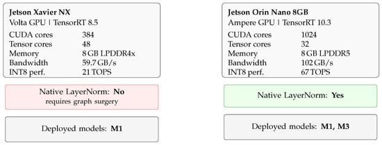
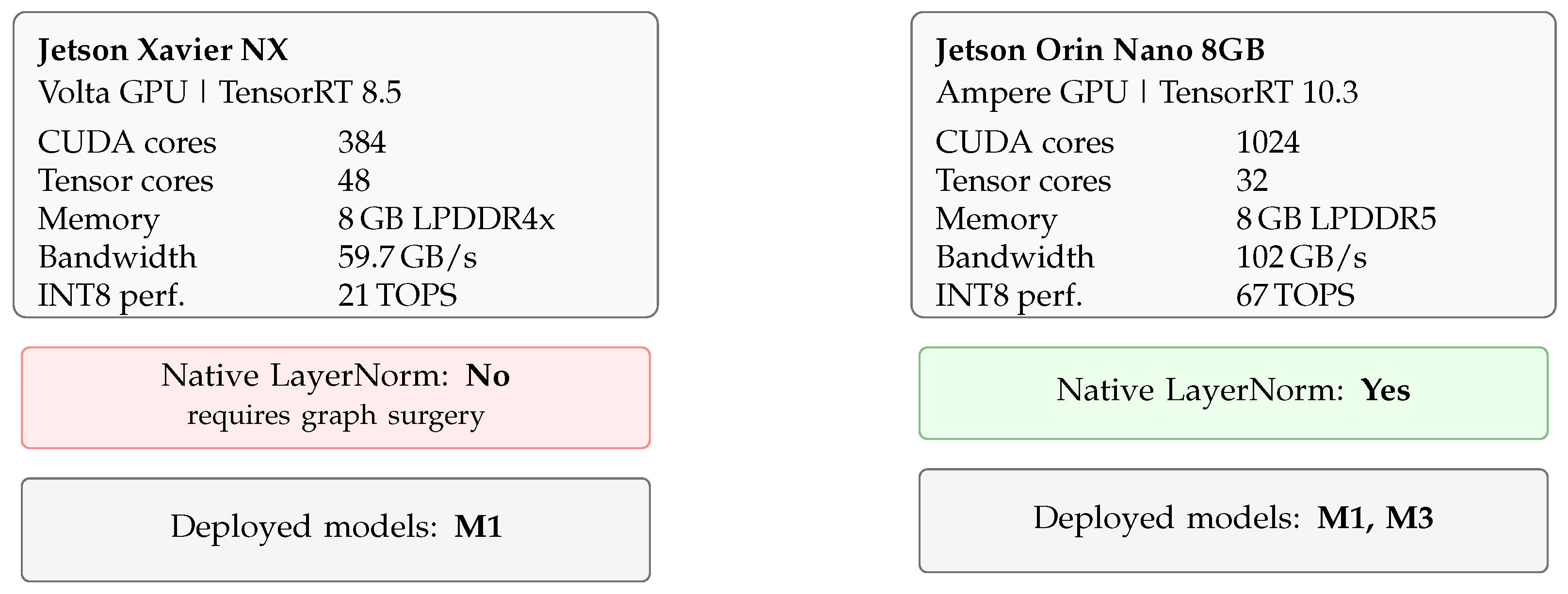




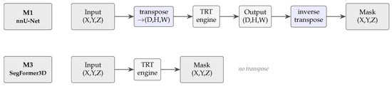
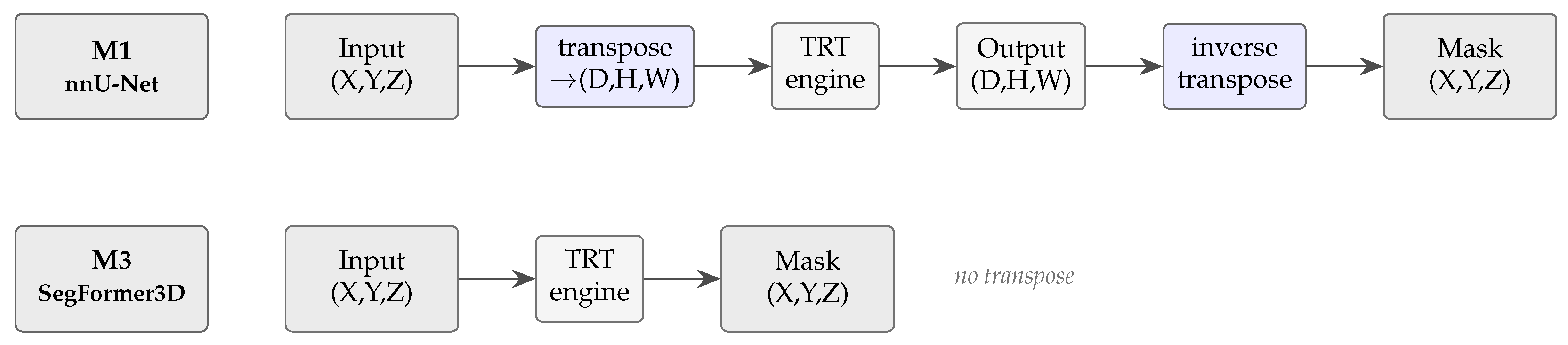
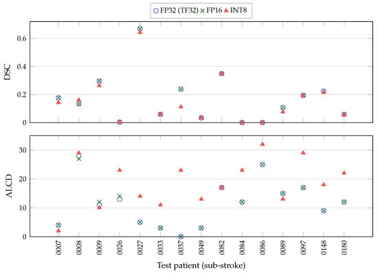
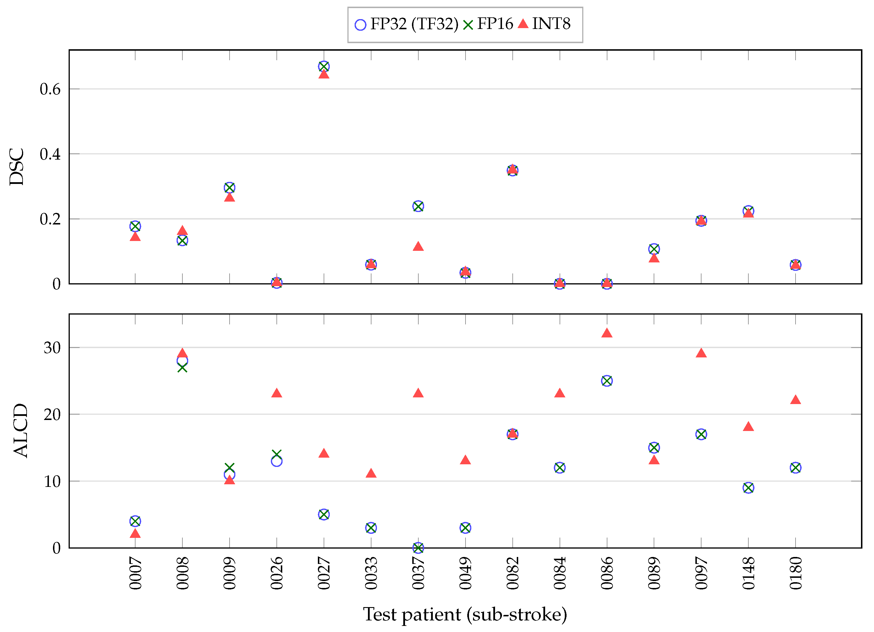
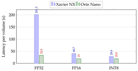
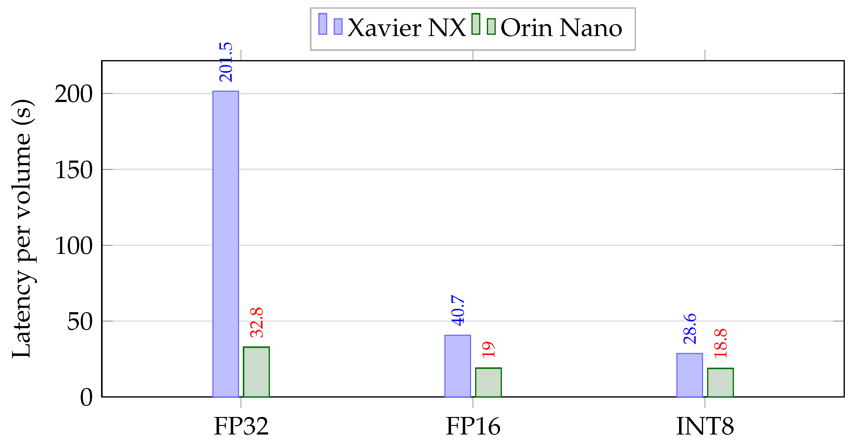
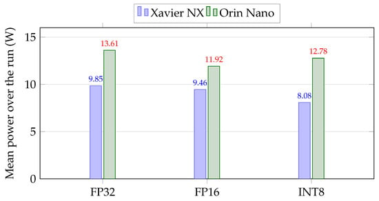
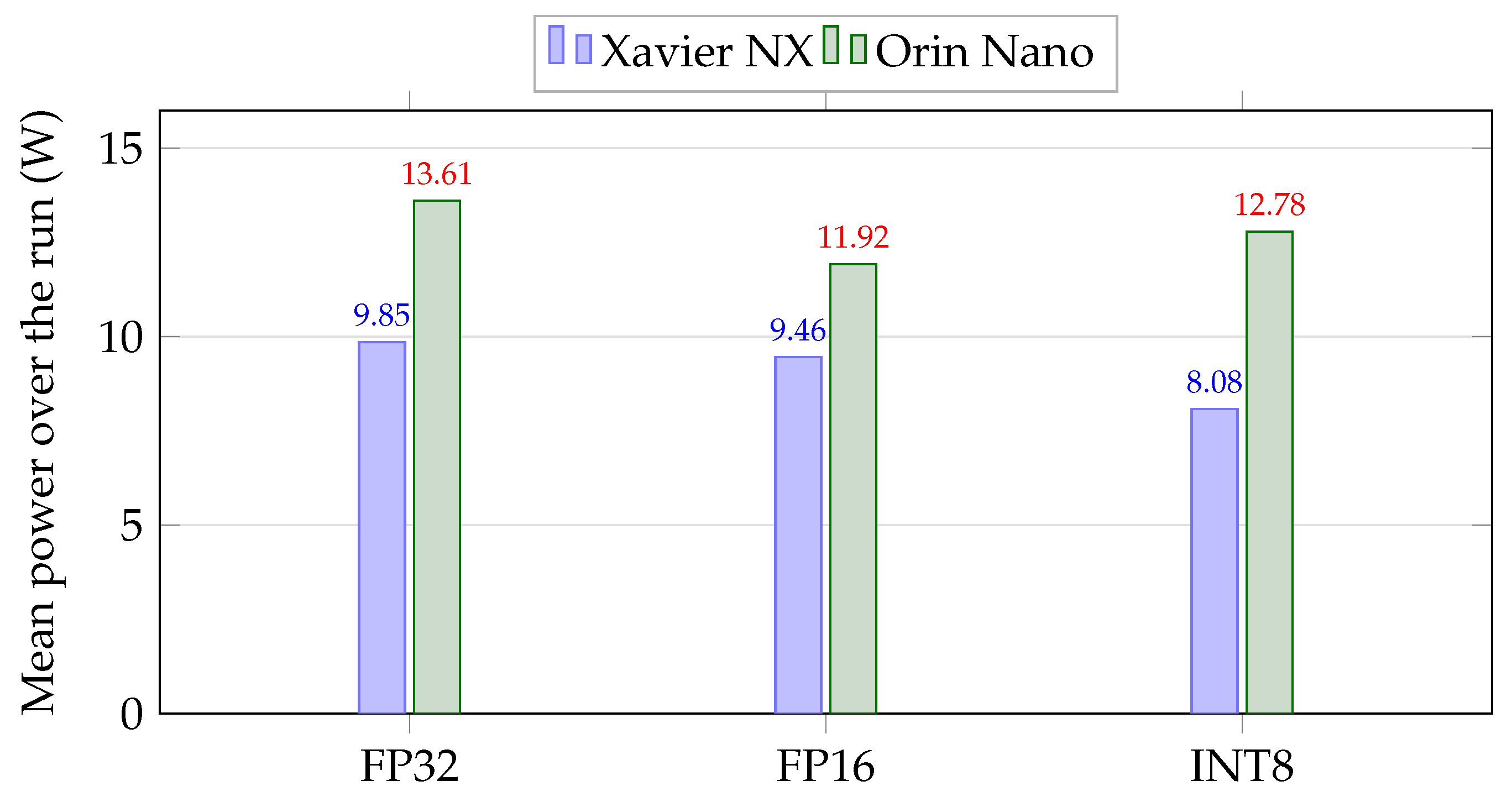

Disclaimer/Publisher’s Note: The statements, opinions and data contained in all publications are solely those of the individual author(s) and contributor(s) and not of MDPI and/or the editor(s). MDPI and/or the editor(s) disclaim responsibility for any injury to people or property resulting from any ideas, methods, instructions or products referred to in the content. |
© 2026 by the authors. Licensee MDPI, Basel, Switzerland. This article is an open access article distributed under the terms and conditions of the Creative Commons Attribution (CC BY) license.