


Abstract
Ship detection in optical and synthetic aperture radar (SAR) imagery supports maritime surveillance and vessel traffic monitoring across different sensing conditions. A common detector can reduce parameter duplication across these modalities, but their different image statistics complicate joint learning from independently annotated, unpaired images. We address this mismatch with SeaBridge-MC, whose private input stems and residual-stage batch normalization (BN) provide modality-specific transformations while residual convolutions, the multiscale encoder, query decoder, and prediction heads remain shared. This allocation increased mean COCO average precision (AP) over full sharing by 18.96 points on LEVIR-Ship and 7.01 points on OSSDD-VH across five matched seeds with BN running statistics updated during training while adding 38,368 trainable parameters (0.1910%). The fully shared detector achieved higher mean optical AP with fixed BN running statistics. Relative to two independent detectors, the joint model used 49.90% fewer total parameters, with lower AP in both domains across three common seeds. SeaBridge-MC therefore offers a compact alternative to separate sensor-specific detectors, enabling unpaired optical and SAR datasets to support a common ship-detection model.
1. Introduction
Optical and synthetic aperture radar (SAR) ship detection supports maritime surveillance and traffic monitoring under different sensing conditions [1,2]. Optical images provide vessel appearance and scene context, whereas SAR observations are less dependent on illumination and cloud cover [3]. Independently annotated images from both modalities support a common ship-detection task. Their common prediction objective permits shared detection modules, while the different image statistics motivate modality-specific transformations in the feature extractor.
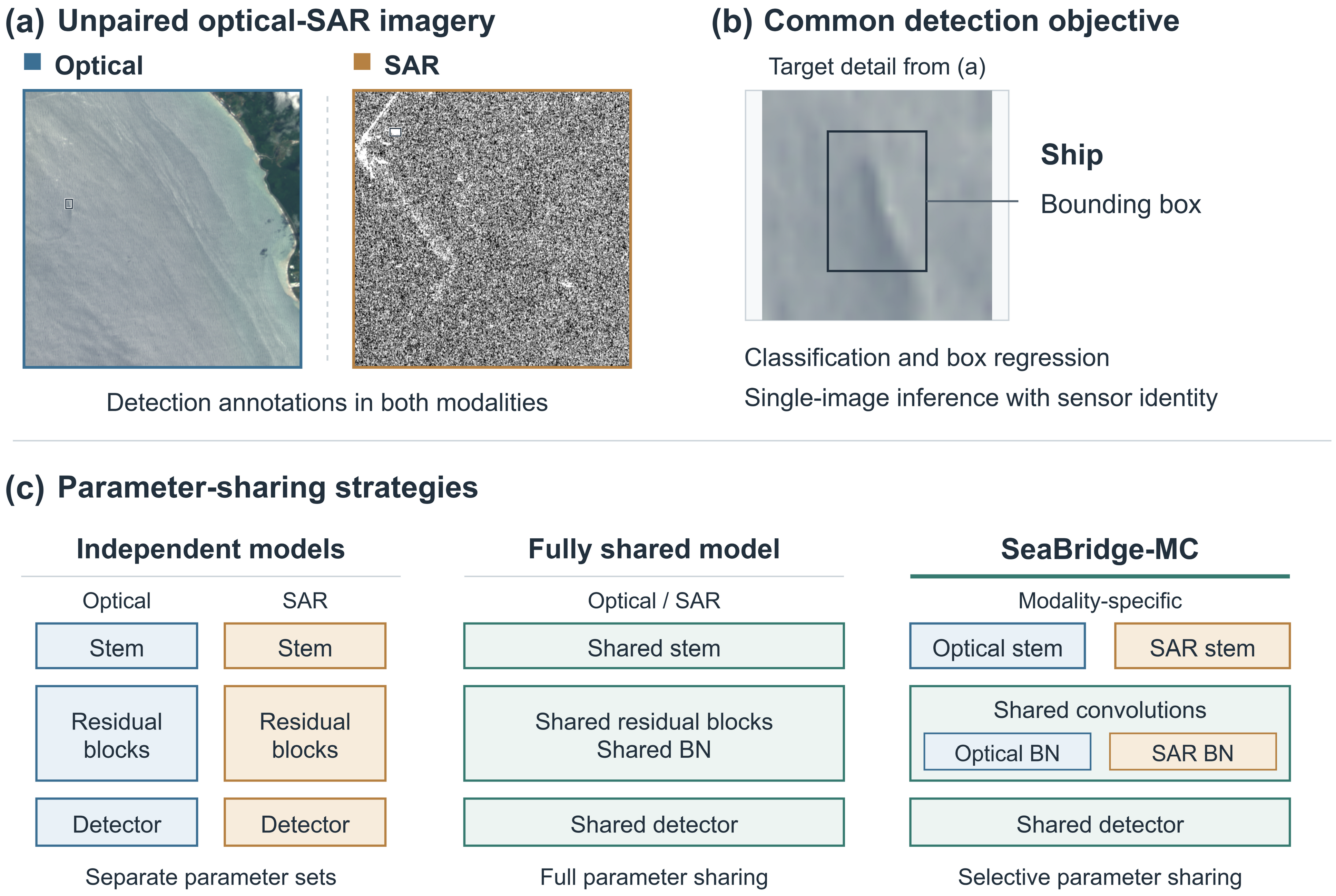
We consider jointly supervised ship detection from optical and SAR collections without scene-level correspondence. Both collections provide one-class annotations with axis-aligned boxes, so a common classifier and box regressor can serve both modalities. Orientation-aware detection extends this output space through angle parameterization and periodicity-aware regression [4,5]. Each inference uses one image and its sensor identifier. The available supervision comprises independent annotations from both modalities, whereas paired optical–SAR fusion uses corresponding observations [6,7], and optical-to-SAR adaptation can use limited target labels [8]. Figure 1 shows the resulting choices between independent models, unconditional sharing, and selective allocation of private parameters.
Figure 1.
Unpaired optical–SAR detection and parameter sharing. (a) Independently annotated, unpaired images. (b) A common ship-detection objective, illustrated by an enlarged target and its ground-truth box from (a). (c) Independent models, unconditional sharing, and SeaBridge-MC. Blue, ochre, and green indicate optical-private, SAR-private, and shared components. Each inference uses one image with known modality. The diagrams indicate which parameters are private or shared.
Image statistics vary even between SAR platforms, affecting detector transfer [9,10]. Domain-specific batch normalization (BN) and residual adapters retain domain-dependent transformations within shared models [11,12]. Shared convolutions with private normalization have also been used for supervised segmentation of unpaired multimodal images [13]. These designs provide a basis for separating sensor-dependent input transformations and normalization from shared detection computation.
Unified remote-sensing detectors also allocate parameters to accommodate heterogeneous detection outputs. SM3Det combines expert routing with task-specific heads [14]; Hua et al. use separate heads for oriented optical boxes and horizontal SAR boxes [15]. A common ship category and horizontal-box representation permit shared prediction heads, concentrating the design question on modality-specific processing within the feature extractor.
We propose SeaBridge-MC, which combines private input stems and modality-specific normalization in residual Stages 1–4 with shared residual convolutions, multiscale encoding, query decoding, and prediction heads. The shared modules receive ground-truth supervision from both collections, while the private branches retain sensor-specific input transformations and normalization.
The main contributions of this study are summarized as follows.
- We propose a modality-conditioned parameter-sharing architecture for jointly supervised optical–SAR ship detection. Private input stems and normalization in all four residual stages retain modality-dependent transformations, while the residual convolutions and encoder–decoder prediction modules remain common.
- SeaBridge-MC improves optical and SAR average precision (AP) over unconditional sharing across five matched seeds with BN running statistics updated during training, reducing the mean absolute cross-dataset AP gap by 37.0%. The combined design also achieves higher mean AP in both domains than either private component alone across three common seeds.
- The RT-DETRv2 implementation adds 38,368 trainable parameters (0.1910%) over full sharing and has a counted computational cost of 94.307 billion floating-point operations (GFLOPs). Its reduced total parameter count relative to independent detectors comes with lower AP, and its accuracy advantage over full sharing depends on the BN setting.
2. Related Work
2.1. Ship Detection Across Optical and SAR Sources
Deep object detection combines learned representations with classification and localization objectives [16]. Feature pyramid networks construct multiscale features [17]. Focal loss reduces the contribution of well-classified examples to address foreground–background imbalance [18]. In optical remote sensing, DIOR documents substantial variation in object scale, orientation, and appearance [19]; LEVIR-Ship focuses on tiny vessels against complex backgrounds [1]. RoI Transformer learns oriented regions from horizontal proposals, and S2A-Net aligns deep features with oriented anchors [4,5]. Both designs explicitly model object orientation in the detection output.
SAR detection must contend with sea clutter, speckle, and weak target-to-background contrast [2,3]. Approaches based on constant false-alarm rate (CFAR) detection address radio interference or combine steady detection with knowledge-oriented classification [20,21]. Learned alternatives include contextual transformer representations [22], receptive-field enhancement with cross-layer fusion [23], and dynamic feature refinement for inshore targets [24]. Space-frequency selection convolution diversifies SAR features through spatial and frequency-domain processing [25]. These advances develop SAR-specific representations through contextual, spatial, and frequency-domain processing.
Dataset scale and annotation granularity also vary across optical and SAR benchmarks. ShipRSImageNet provides fine-grained optical ship categories [26]. HRSID supports SAR detection and instance segmentation [27]. Acquisition differences further affect transfer between sources of the same sensor type. Zhao et al. separate source-specific knowledge from transferable representations in multisource satellite-borne SAR detection [9], and Liu et al. address platform shift through confusion-corrected self-training and region-aware alignment [10]. Both studies address acquisition-dependent variation within SAR imagery through source-specific representations or cross-platform alignment.
2.2. Correspondence-Based Learning and Domain Adaptation
Correspondence-based multimodal learning uses observations of a common scene to construct a joint representation or prediction. The bridge neural network learns from co-registered optical and SAR images for joint interpretation [6]. MHFNet accommodates imperfect registration through alignment, uncertainty-aware losses, and decision-level fusion but still operates on observations of the same scene [7]. CROMA and SkySense V2 likewise exploit spatial, temporal, or geographic correspondence during multimodal representation learning [28,29]. Their training signals draw on correspondence across sensor observations.
Visible–infrared detectors use jointly available observations to construct fused predictions. SuperYOLO combines pixel-level multimodal fusion with a super-resolution training branch [30]. SGFNet uses semantic feedback for fusion, and IAF-RTDETR conditions visible–infrared fusion on illumination estimates [31,32]. These designs combine information from paired visible and infrared inputs.
Domain adaptation uses different levels of supervision in the source and target domains. Domain Adaptive Faster R-CNN aligns image- and instance-level representations using labelled source and unlabelled target images [33]. SAR-CDSS incorporates limited target labels; source-free adaptation constructs pseudo-labels without retaining source images [8,34]. Other approaches generate SAR-like training images [35], use inversion regularization [36], or introduce semantic prompts to reduce the source–target mismatch [37]. Jointly supervised detection instead uses ground-truth annotations from both domains to train a common detector.
2.3. Private Interfaces and Shared Detection Models
Private interfaces retain domain-dependent transformations within shared models. Domain-specific batch normalization (BN) separates normalization statistics and affine parameters [11]; residual adapters add private residual transformations [12]; cross-stitch units combine task activations [38]. Chen et al. combine shared convolutions, modality-specific normalization, and class-specific affinity constraints for labelled, unpaired multimodal medical-image segmentation [13]. Wang et al. use private encoder normalization with shared convolutions and bidirectional feature fusion for pixel-aligned multimodal dense prediction [39]. The shared/private boundary therefore varies across these designs, from normalization and residual transformations to feature interactions.
Remote-sensing models extend selective sharing across heterogeneous collections. msGFM uses sensor-specific embeddings and decoders around a shared encoder, accommodating paired and unpaired sensor data [40]. SM3Det combines grid-level sparse mixture-of-experts routing with task-specific detection heads across spatially unaligned datasets [14]. These models accommodate sensor heterogeneity while retaining sensor- or task-dependent outputs.
Hua et al. address ship detection from unpaired optical and SAR images [15]. Their framework combines independent stems, shared and dedicated experts, balanced region-feature sampling, category-level contrastive learning, and dynamic loss weighting. Its Up-Det benchmark uses optical oriented boxes from DOTA and horizontal SAR boxes from SARDet-100K [41], with separate detection heads. SeaBridge-MC uses a common ship class and horizontal-box representation, keeping the prediction heads shared and assigning modality-specific parameters to the input stems and BN in all four residual stages.
3. Materials and Methods
3.1. Task Definition and Experimental Scope
Let index the optical and synthetic aperture radar (SAR) modalities. Each modality provides a labelled detection set , where is the ith input image from modality m and is the number of images from modality m. The annotation contains retained instances, with class label and axis-aligned box for instance k. No mapping between the indices of and is available or constructed. Both datasets contribute supervision through independently sampled images.
The detector is denoted by , where contains the shared parameters and normalization state, and contains their modality-specific counterparts. These collections include both trainable parameters and non-trainable normalization state; parameter counts include only trainable tensors. Each input image is accompanied by its known modality identifier. All datasets are converted to a common one-class label space with horizontal bounding boxes. The alternative allocations of shared and modality-specific parameters use this common label space and output definition.
The primary comparison evaluates a fully shared detector and SeaBridge-MC on LEVIR-Ship and OSSDD-VH across five seeds. The fully shared reference is labelled N in the feature-diagnostic figure. Component and shared-capacity comparisons use the common seed subset 2001–2003.
3.2. Detector Backbone and SeaBridge-MC
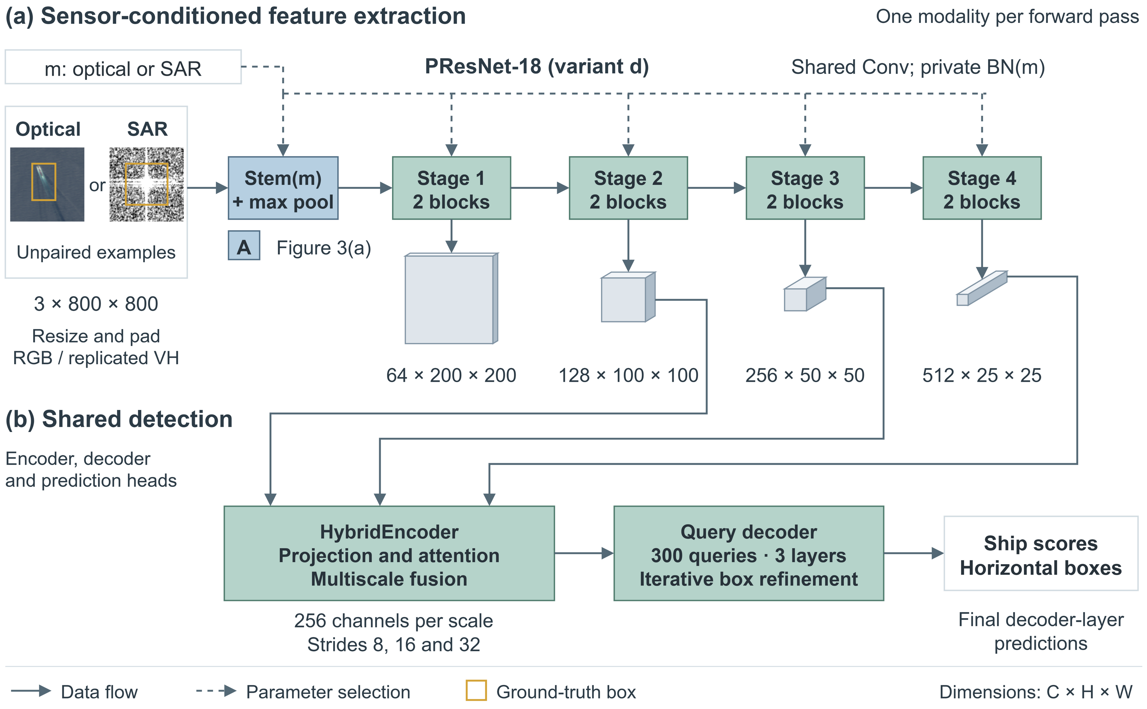
SeaBridge-MC modifies RT-DETRv2-R18 with a PResNet-18 variant-d backbone, a 256-dimensional HybridEncoder, and a three-layer query decoder [42,43]. The backbone follows residual learning with the variant-d refinements [44,45]. The encoder receives three backbone levels with output strides 8, 16, and 32. The decoder maintains 300 object queries and predicts one foreground class. SeaBridge-MC uses modality-private input stems and normalization paths throughout the residual backbone. All residual convolutions, the multiscale encoder, query decoder, and prediction head remain shared. Table 1 identifies the shared and modality-specific components.
Table 1.
Parameter sharing in SeaBridge-MC.
For residual stage , the forward map is
where denotes the feature representation for modality m after residual stage l, , and selects the three encoder input levels. is the stem with private parameters , is a residual stage, and contains its modality-specific BN branches. is the encoder, denotes the query decoder and prediction heads, and is the set of predicted class scores and boxes. The residual convolution parameters , encoder parameters , and decoder and prediction-head parameters belong to . The private set is . Each input stem includes its own normalization layers; normalization outside the stem and residual backbone remains shared.
The selected backbone outputs have 128, 256, and 512 channels, respectively. Detection follows the Detection Transformer (DETR) query-based set-prediction formulation, with multiscale sampling based on deformable attention [46,47]. For modality m, the shared decoder returns . The predictions and denote the ship score and horizontal box for query q. Figure 2 separates sensor-conditioned backbone processing from the shared multiscale encoder, query decoder, and prediction heads.
Figure 2.
SeaBridge-MC architecture. (a) Modality-specific stems and normalization with shared residual convolutions (Figure 3). (b) A shared multiscale encoder, query decoder, and prediction heads. Solid arrows indicate data flow; dashed arrows indicate component selection controlled by the known modality m. Cuboid dimensions denote channels × height × width. Unpaired optical and SAR crops illustrate the inputs; gold boxes mark the ground-truth annotations. Auxiliary training outputs and denoising queries are omitted.
3.2.1. Modality-Private Input Stems
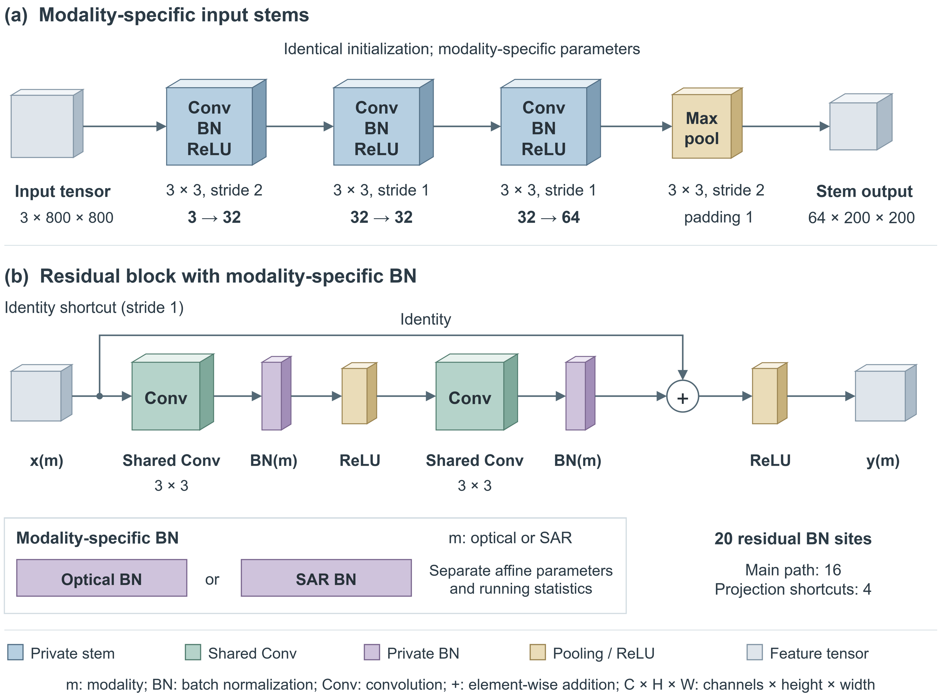
The private input stems provide modality-specific initial spatial transformations before the common detection modules. The PResNet variant-d stem contains three convolution–normalization–activation blocks with channels . The arrows indicate the input and output channel counts of successive convolutions. The convolution strides are 2, 1, and 1, followed by stride-2 max pooling. An image therefore produces a stem output, with dimensions ordered as channels, height, and width. SeaBridge-MC maintains a separate copy of this complete stem for each modality, including its normalization parameters and running statistics. Both first convolutions accept three channels; the SAR input contains one normalized vertical-transmit/horizontal-receive (VH) measurement replicated across all three channels.
The SAR stem is initialized as an exact copy of the optical stem after compatible pretrained tensors have been loaded. For the first convolution,
The remaining stem tensors are also copied, after which the two stems are updated independently. This initialization preserves the original stem response to the replicated SAR input without averaging its channels or summing kernel channels. The additional three-channel stem contributes 28,768 trainable parameters. No image translation or cross-route feature fusion is applied.
Figure 3.
Modality-specific stems and normalization. (a) Identical stem architectures with separate weights and BN states. Channel arrows denote input-to-output channels; the three convolutions use strides 2, 1, 1, followed by stride-2 pooling. An input produces a output (channels × height × width). (b) Shared convolutions and modality-specific BN in an identity-shortcut residual block; projection shortcuts are omitted. The inset distinguishes trainable BN affine parameters from non-trainable running statistics. Modality m selects the BN state; , , and + denote input, output, and element-wise addition. Private indicates modality-specific parameters and normalization state; colors identify component types.
3.2.2. Residual-Stage Modality-Specific Normalization
Private residual-stage normalization introduces sensor-dependent channel transformations beyond the input stem; the convolutional kernels remain shared. Each of the 20 two-dimensional batch-normalization modules inside the four residual stages is replaced by two independently updated branches [11,48]. For activation z, module j, and modality m, the transformation is
where ⊙ denotes element-wise multiplication, is the numerical-stability constant, and and are modality-specific trainable affine parameters. The mean and variance are mini-batch statistics during training and running estimates during evaluation. Running statistics are stored as non-trainable buffers. Training updates only the BN branch selected by the input modality. BN modules in the shared encoder retain common affine parameters and running statistics.
The duplicated residual-stage normalization paths add 9600 trainable parameters. Together with the private stems, they add 38,368 parameters in SeaBridge-MC. The input modality selects a single BN branch. Figure 3 shows the private stem topology and an identity-shortcut residual block with shared convolutions and modality-specific normalization. The residual stages contain 16 main-path BN sites and four projection-shortcut BN sites, each maintaining separate optical and SAR states.
3.3. Joint Objective and Parameter Initialization
RT-DETRv2 assigns predicted queries to reference boxes through Hungarian matching. The matching costs for classification, , and generalized intersection-over-union (GIoU) are weighted 2, 5, and 2, respectively. Following assignment, the loss optimized for each domain combines varifocal loss (VFL), , and GIoU terms:
where contains the final decoder output and auxiliary decoder, denoising, and encoder outputs. The VFL term [49] uses and ; box regression combines and GIoU losses [50]. Training uses 100 denoising queries, a label-noise ratio of 0.5, and a box-noise scale of 1.0.
Each joint update uses eight optical images and eight SAR images. Gradients from the two domain losses are accumulated before a single optimizer step:
Each term in Equation (5) uses annotations from its own domain. The fully shared RT-DETRv2 reference retains its original shared batch-normalization modules.
Compatible tensors were loaded by matching names and shapes against the RT-DETRv2-R18 COCO checkpoint. Task-head tensors with incompatible shapes retained their detector initialization, and both route-specific normalization paths began from the same matched checkpoint state.
3.4. Datasets, Derived Partitions, and Input Processing
Primary Datasets and Partitions
The datasets comprise LEVIR-Ship optical images and OSSDD-VH Sentinel-1 chips [1,51]. Both datasets provide ship annotations from distinct scenes and acquisition times. Sensor and dataset source therefore vary together in this comparison.
LEVIR-Ship is partitioned by acquisition-source groups derived from product identifiers. Removing the terminal tile-coordinate pair _x_y gives 114 segment identifiers; merging terminal hyphen-number segment suffixes gives 71 source groups. Training, validation, and test contain 50, 7, and 14 disjoint source groups, respectively. Byte-identical image screening found no cross-partition duplicates; four near-duplicate candidates were distinct acquisitions sharing no-data borders. The resulting train, validation, and test sets contain 2677, 397, and 822 images. Their respective ship-box counts are 2209, 353, and 657.
OSSDD-VH uses a scene-disjoint partition derived from the downloadable metadata. Four metadata records were reassigned from the test partition to the training partition so that each scene occurred in only one partition. The resulting train, validation, and test sets contain 10,670, 1459, and 3032 chips from 20, 3, and 16 scenes. Valid coordinate rows were retained as boxes. Count and identifier anomalies in the source metadata were recorded without imputation. Table 2 summarizes both data partitions.
Table 2.
Dataset partitions and annotation counts.
Optical training applied horizontal flipping with probability 0.5. Images were resized isotropically so that the longer side equalled 800 pixels, then padded on the right and bottom to . Boxes smaller than one pixel after transformation were removed. Retained boxes were represented as normalized . Validation and test omitted the random flip.
For each OSSDD-VH array v, intensities were normalized as
where and are the per-image percentiles computed after the logarithmic transform. The normalized values were rounded to 8-bit intensity and replicated across three channels for both the fully shared model and SeaBridge-MC. SAR training used crops with identical geometric transformations applied to each image and its boxes; crop origins were determined by crop seed 0, the budget-unit index, and the image filename. Cropping preceded horizontal flipping (probability 0.5), isotropic resizing, and right/bottom padding to . Validation and test converted each native chip into an detector input using the same deterministic resizing and padding.
3.5. Controlled Variants and Training Protocols
The experiments compare complete sharing, private input stems, private residual-stage BN, their combination in SeaBridge-MC, and a parameter-matched shared residual branch (Table 3). In the standard setting, BN affine parameters are optimized and running statistics are updated during training. Shared BN processes two successive batches of eight images per joint update; each private BN branch processes one batch of eight from its corresponding modality.
Table 3.
Configurations for the component comparisons. Parameter increments are relative to the fully shared detector; residual convolutions, encoder, decoder, and heads are shared in all joint configurations.
3.5.1. Primary Five-Seed Mixed-Precision Protocol
The primary comparison trained the fully shared model and SeaBridge-MC with model seeds 2001–2005. Each optimizer update accumulated gradients from eight optical images followed by eight SAR images, with equal weighting of the two domain losses. Within each seed, all configurations used the same batches and augmentation sequence for each modality. Separate random seeds were derived for source-model initialization, initialization of each architectural variant, and training. Each run comprised ten budget units of 2000 successful joint optimizer updates, for a total of 20,000 updates.
AdamW [52] used . Target learning rates were for the configured non-normalization backbone group and for the remaining groups. Linear warm-up advanced over 1000 successful updates. The cosine scheduler used and a minimum rate of , advancing once at the end of each 2000-update budget unit rather than after every optimizer update. Weight decay was , except for the separately grouped encoder and decoder normalization parameters, which used zero decay. Gradients were clipped at an norm of 1.0. Forward computation used bfloat16 (BF16) autocast with 32-bit floating-point (FP32) master parameters and loss reductions; the criterion ran outside autocast, and no gradient scaler was active. Exponential moving average (EMA) advanced only after successful updates with decay , including floating-point normalization state. Integer buffers retained their initial values. BN momentum was fixed at 0.1, so the averaging factor was independent of the batch counter.
Checkpoints were saved every 2000 updates and validation was performed every 4000 updates. All ten primary runs reached 20,000 updates. Fixed seeds and matched data order enabled paired comparisons across configurations.
3.5.2. Component and Shared-Capacity Controls
The component configurations used LEVIR-Ship and OSSDD-VH with the primary mixed-precision protocol. The private-stem model retained private three-channel input stems, including their normalization layers, but shared residual-stage normalization; the private-residual-BN model retained a shared stem but used private residual-stage normalization; SeaBridge-MC combined the private stems and residual-stage normalization. The stem and residual-normalization increments were 28,768 and 9600 trainable parameters, respectively. The shared-capacity model added a shared residual branch with 38, 368 trainable parameters after the common stem, matching the parameter increment in SeaBridge-MC. The branch combined a bottleneck and 60-channel offset with a zero-initialized, 64-channel depthwise convolution.
The private-stem, private-residual-BN, and shared-capacity models used the common seed subset 2001–2003 with the primary initialization, data order, optimizer, and validation-selection settings. Each configuration was compared with the fully shared model and SeaBridge-MC using the corresponding runs for the same seeds.
The fully shared model contains 20,083,028 trainable parameters. SeaBridge-MC contains 20,121,396 parameters, adding 38,368 (0.1910%).
3.5.3. Order, Normalization, and Independent-Training Comparisons
Forward order was optical-first, SAR-first, or randomized for both joint architectures over seeds 2001–2003. In the default setting, BN computes training batch statistics and updates the running buffers. An additional optical-first condition fixed the running mean and variance of every BN module at initialization while retaining trainable affine parameters. Each condition used 20,000 successful updates and the primary per-domain data order, augmentation, and optimizer settings.
Independent optical and SAR detectors used seeds 2001–2005, the same initialization source, and 20,000 updates of 8 images from their own domain (160,000 image exposures per domain). Each independent detector used its domain loss with unit weight; joint training weighted each domain loss by 0.5. Each independent detector was selected by its own validation AP over the same five checkpoints; joint detectors used validation . The original five-seed runs, additional three-seed joint runs, and five-seed independent runs were analysed separately. Alternative criteria for joint-checkpoint selection were optical validation AP and SAR validation AP; each selected checkpoint was evaluated on both domains.
3.6. Evaluation and Statistical Analysis
For the primary protocol, checkpoint selection maximized the harmonic mean of optical and SAR validation AP among updates 4000, 8000, 12,000, 16,000 and 20,000. Ties were resolved in favour of the earlier checkpoint. For optical and SAR COCO AP values and , respectively, the harmonic mean is
Optical and SAR AP were the primary outcomes; summarized joint performance and was used for checkpoint selection. AP is computed separately for each modality over intersection-over-union (IoU) thresholds 0.50 to 0.95 in increments of 0.05 [53]. The primary analysis used all five seeds to compute sample means, sample standard deviations, and paired differences defined as SeaBridge-MC minus the fully shared model. Harmonic means and absolute cross-dataset AP gaps are computed within each seed before aggregation. The component analysis compared the five configurations over the common seeds 2001–2003, including paired differences between SeaBridge-MC and each of the private-stem, private-residual-BN, and shared-capacity models.
Evaluation used the RT-DETRv2 COCO bounding-box evaluator implemented with faster-coco-eval 1.7.2. Sigmoid class scores were used to retain the top 300 predictions per image, without an additional score cutoff or NMS. COCO maxDets was [1,10,100], with the main AP evaluated at 100. Inference used FP32 with autocast disabled. Normalized predictions were scaled to original-image coordinates and converted to COCO . Test partitions had been evaluated in the original study; all additional checkpoints and selection rules were determined from validation data. The absolute cross-dataset AP gap is .
3.7. Feature Responses and Gradient Alignment
We examined spatial attribution, foreground–background responses, and cross-modal gradient alignment as complementary diagnostics of the shared backbone. All analyses used frozen EMA checkpoints and the original validation preprocessing, with no detector updates. A fixed hash ordering selected 128 ship-containing validation images per modality and one ground-truth ship per image. Each ship box was paired with an equally sized region from the same image that did not intersect any annotated ship. Region-of-interest (ROI) features from Stages 3 and 4 were pooled to a grid with ROIAlign, and spatial averaging produced 256- and 512-dimensional descriptors, respectively. A binary logistic probe ( regularization, ) measured ship–background discrimination using three source-group-disjoint folds covering six optical source groups and three SAR scenes. Standardization and probe fitting used only the training folds. The area under the receiver-operating-characteristic curve (AUROC) was evaluated both from pooled out-of-fold scores and within each held-out fold before equal-weight or ROI-count-weighted averaging.
Image-space attribution used gradient-weighted class activation mapping (Grad-CAM) [54] on a fixed subset of 64 images per modality. The original Hungarian matcher assigned each preselected ground-truth ship to a final-decoder query; the raw ship logit of the matched query defined the attribution target. For feature tensor at layer l, the map was
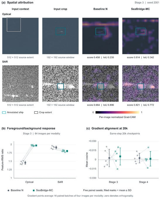
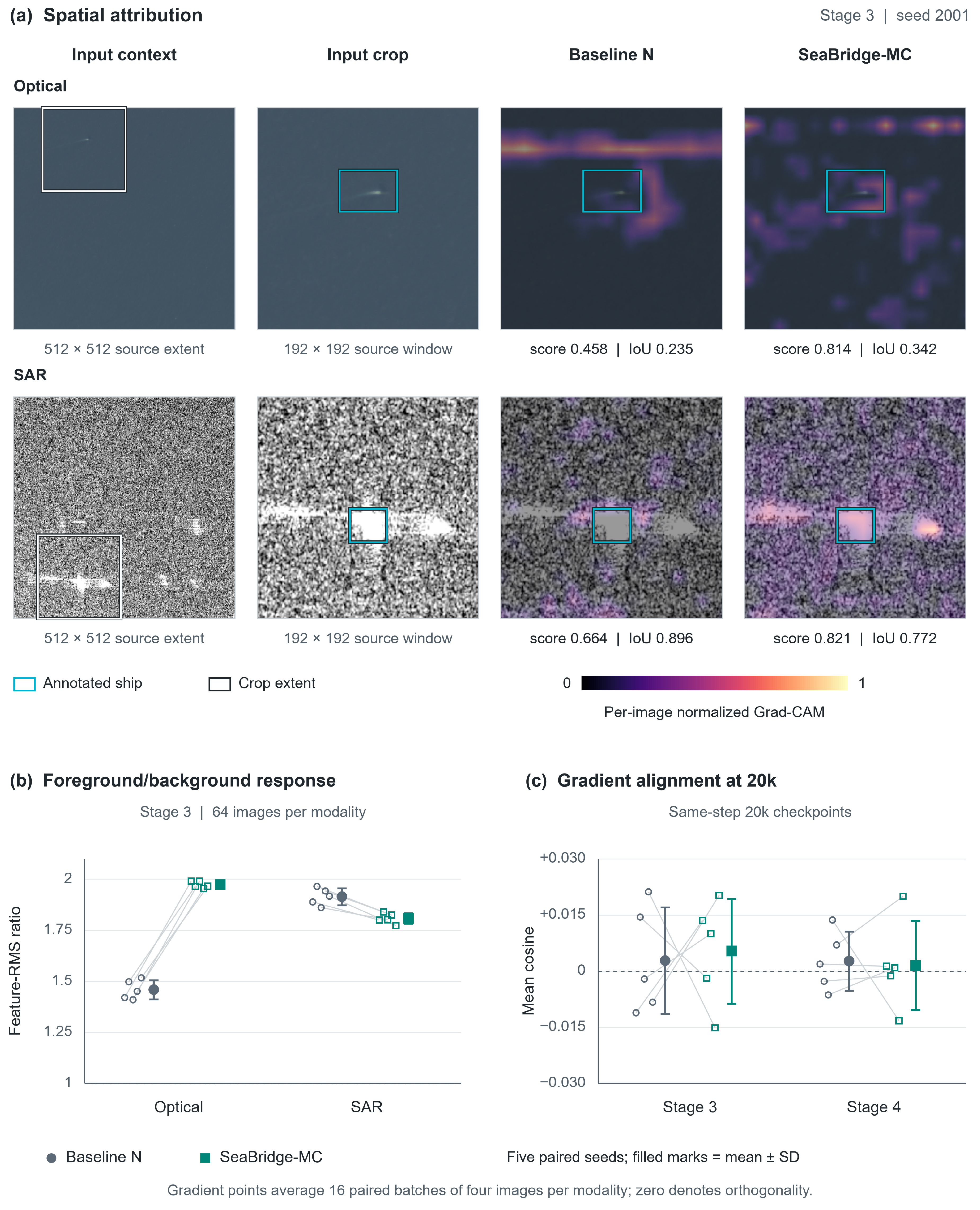
where c indexes feature channels, indexes spatial positions, and are feature-map height and width, and is the spatially averaged logit gradient for channel c. Stage 3 and Stage 4 provided and maps at input strides 16 and 32. Maps were divided by their full-image maximum, bilinearly enlarged to the input canvas, and overlaid with a common color scale and opacity of 0.40; zero maps remained blank. The same -pixel source-image windows were used across models, without renormalization after cropping. Display examples were fixed before attribution by ground-truth area and source-group diversity, with seed 2001 used for illustration. Query scores and box IoU were recorded independently of the maps. Foreground–background activation contrast was quantified from the channelwise root-mean-square (RMS) response at each spatial location. The contrast was defined as the mean ship-ROI response divided by the mean response in an equally sized, nonoverlapping background ROI from the same image, independently of Grad-CAM normalization and display settings.
Gradient alignment was measured separately in the parameter space of the shared Stage 3 and Stage 4 convolutions. The same 64 images per modality formed 16 deterministically ordered batch pairs, with four optical and four SAR images per pair; the batches were not scene-aligned. In evaluation mode, each modality used the final-decoder loss , retaining the original matching and loss definitions. For the shared convolution weights , the gradients and their cosine similarity were computed as
Negative cosine denotes opposing local gradient directions [55]. Private stems and normalization parameters were excluded. The diagnostic used FP32 and frozen normalization state, without auxiliary or denoising losses, gradient clipping, or parameter updates. All five model-seed pairs were evaluated at both the validation-selected checkpoints and the common 20,000-update endpoints to assess checkpoint-timing sensitivity. Batch-level cosine and negative-cosine frequency were summarized within each seed; between-seed variation used the sample standard deviation (SD). These measurements characterize local loss geometry at the evaluated EMA states.
3.8. Implementation Details
Experiments used Python 3.12.13, PyTorch 2.11.0+cu128, torchvision 0.26.0+cu128, and CUDA 12.8. The detector was initialized from the RT-DETRv2-R18 COCO checkpoint. Detection-accuracy evaluations and GPU-forward latency measurements used an RTX 5080 Laptop GPU (NVIDIA Corporation, Santa Clara, CA, USA) in FP32.
4. Results
4.1. Overall Detection Performance and Cross-Dataset Balance
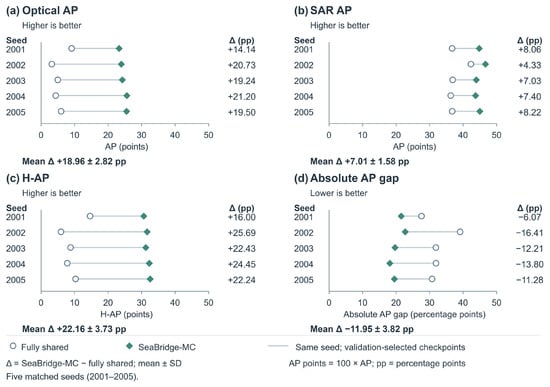
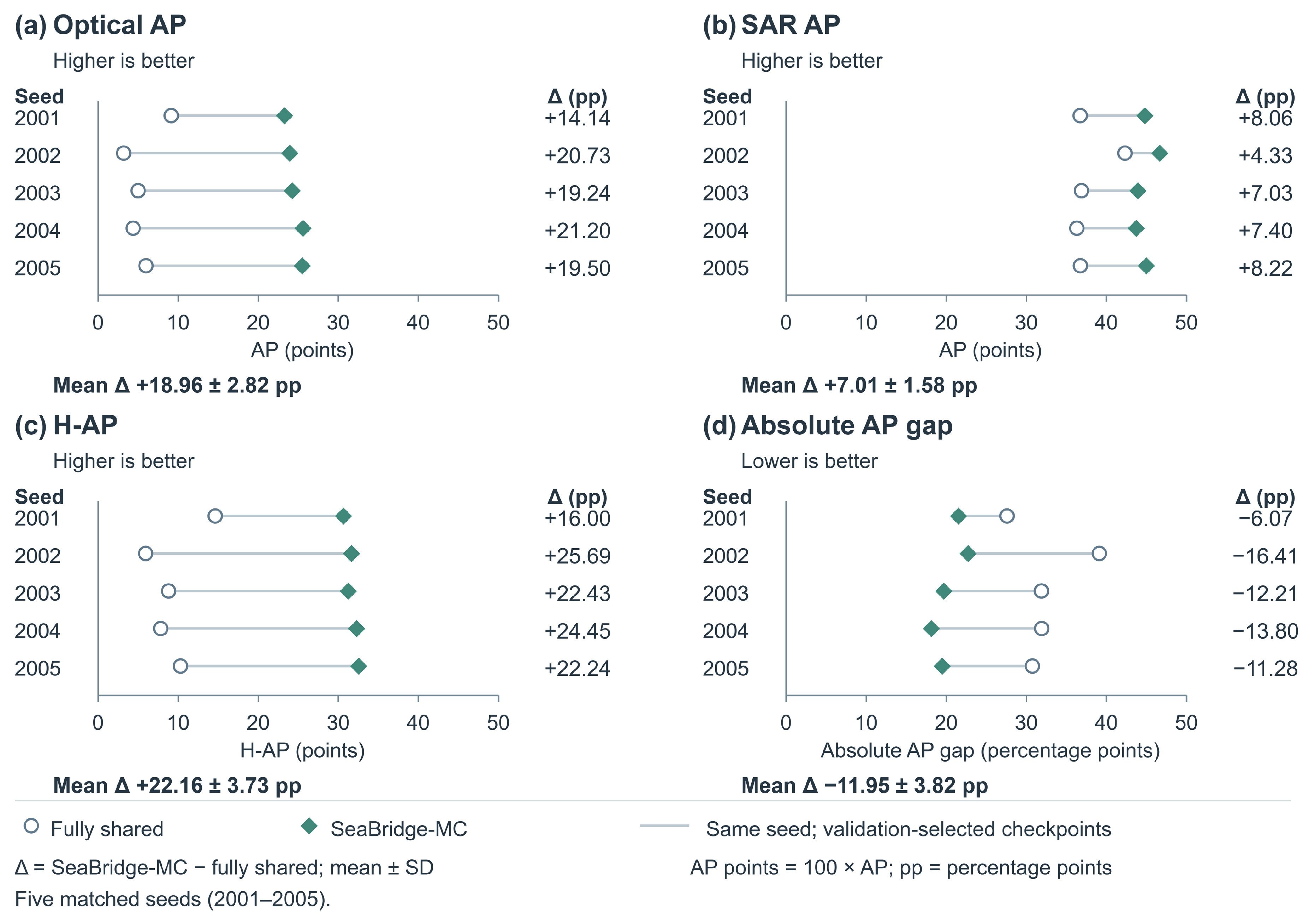
SeaBridge-MC improved AP in both domains in every matched seed. Mean optical AP increased from 0.0555 to 0.2451 and mean SAR AP from 0.3781 to 0.4482, with paired gains of 0.1896 and 0.0701, respectively (Table 4; Figure 4). The increase was larger in the lower-performing optical domain.
Table 4.
Detection accuracy on LEVIR-Ship and OSSDD-VH. Entries are mean ± sample standard deviation (SD) over matched training seeds on the 0–1 scale. and the AP gap are computed within each seed; denotes the paired SeaBridge-MC-minus-fully-shared difference.
Figure 4.
Matched-seed detection performance on LEVIR-Ship and OSSDD-VH. Panels show (a) optical AP, (b) SAR AP, (c) , and (d) absolute AP gap. Blue-grey circles and teal diamonds denote the fully shared model and SeaBridge-MC, respectively, and are linked by seed. Scores are multiplied by 100; paired differences are in AP points. Summary labels report the mean ± sample SD of paired differences. Higher is better in (a–c), and lower is better in (d).
The mean absolute optical–SAR AP gap decreased by 0.1195, from 0.3226 to 0.2031, a relative reduction of 37.0%. The harmonic mean increased from 0.0951 to 0.3167, with the larger AP gain in the lower-performing optical domain contributing more strongly to this increase. The between-seed standard deviations also decreased from 0.0225 to 0.0101 for optical AP and from 0.0254 to 0.0116 for SAR AP. The narrower AP gap and smaller standard deviations indicated improved cross-domain balance and lower between-seed variability under the evaluated protocol.
4.2. Localization Behavior Across IoU Thresholds
The optical AP gain was concentrated at moderate overlap, whereas the SAR gain was larger at the higher IoU threshold (Table 5). SeaBridge-MC increased optical by 0.4846 and by 0.0633; the corresponding SAR increases were 0.0664 and 0.1081. A substantial optical – difference also remained under five-seed independent training (0.7392 versus 0.1039). In the separate seed-2001 optical validation analysis, SeaBridge-MC and the independent detector matched 337 and 346 of 353 ground-truth boxes at IoU 0.50, respectively, with median matched IoU of approximately 0.700 in both cases. Independent training therefore increased the number of matched boxes while giving similar median overlap among matched boxes.
Table 5.
Detection accuracy at IoU thresholds 0.50 and 0.75. Entries are mean ± sample SD over matched training seeds; AP is on the 0–1 scale.
4.3. Optimization Dynamics at a Common Endpoint
SeaBridge-MC retained higher mean AP in both domains than the fully shared model at the common 20,000-update endpoint (Table 6). The validation rule selected update 4000 for four fully shared runs and update 8000 for their SeaBridge-MC counterparts; both models selected update 12,000 for seed 2002. At update 20,000, the optical AP, SAR AP, and advantages were 0.2306, 0.0637, and 0.2207, respectively, with a positive harmonic-mean difference in all five seeds. Continued training increased SAR AP and decreased optical AP for both models. The accompanying decrease in was smaller for SeaBridge-MC: 0.0100, compared with 0.0469 for the fully shared model.
Table 6.
Validation accuracy by checkpoint selection. Entries are mean ± sample SD over training seeds. Selected checkpoints maximize validation ; endpoint checkpoints use 20,000 updates.
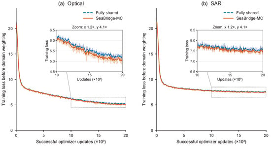
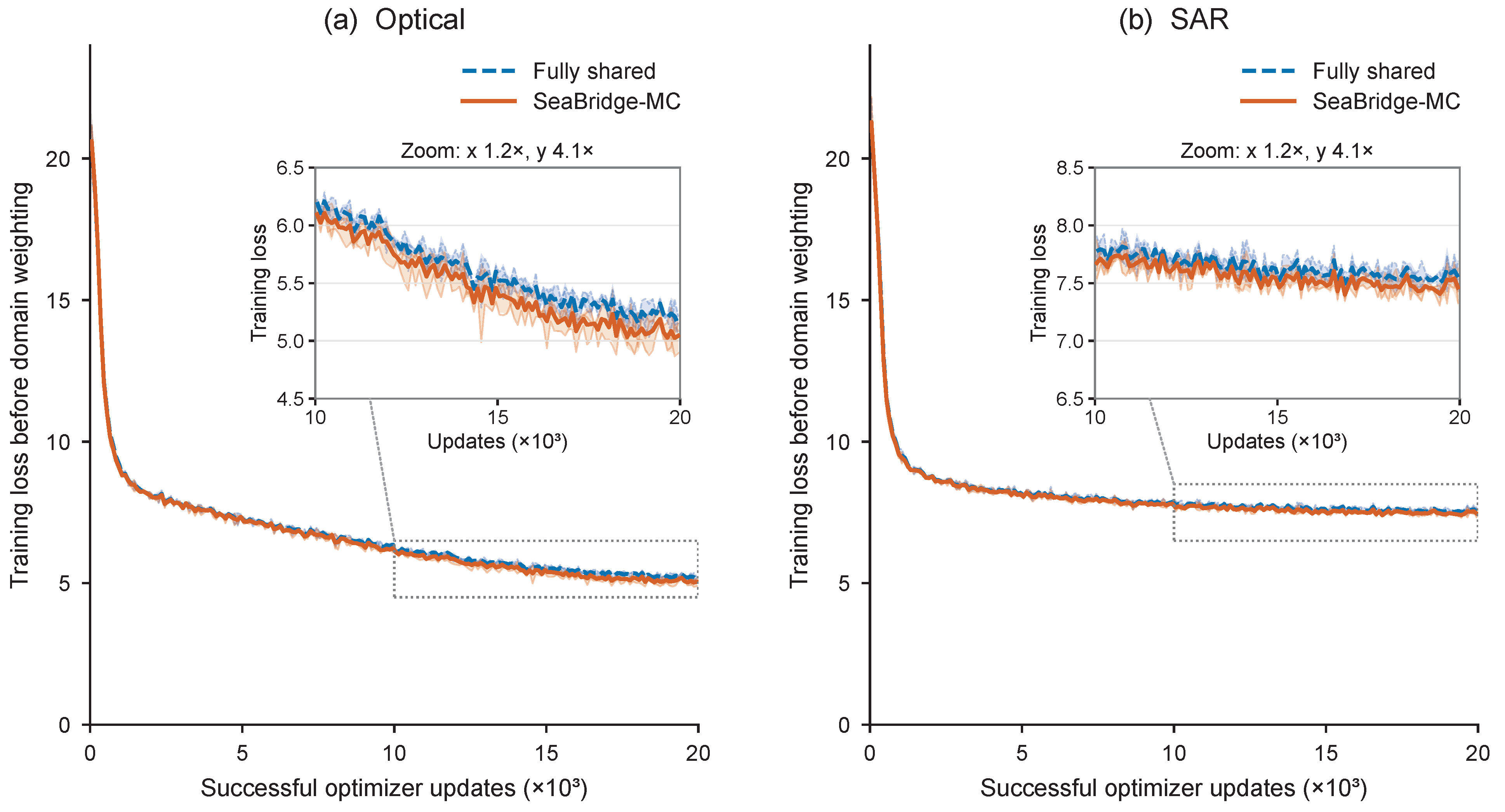
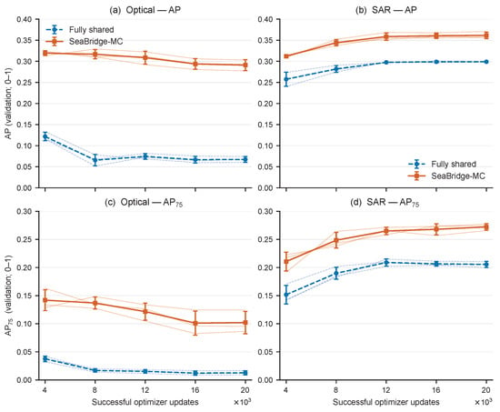
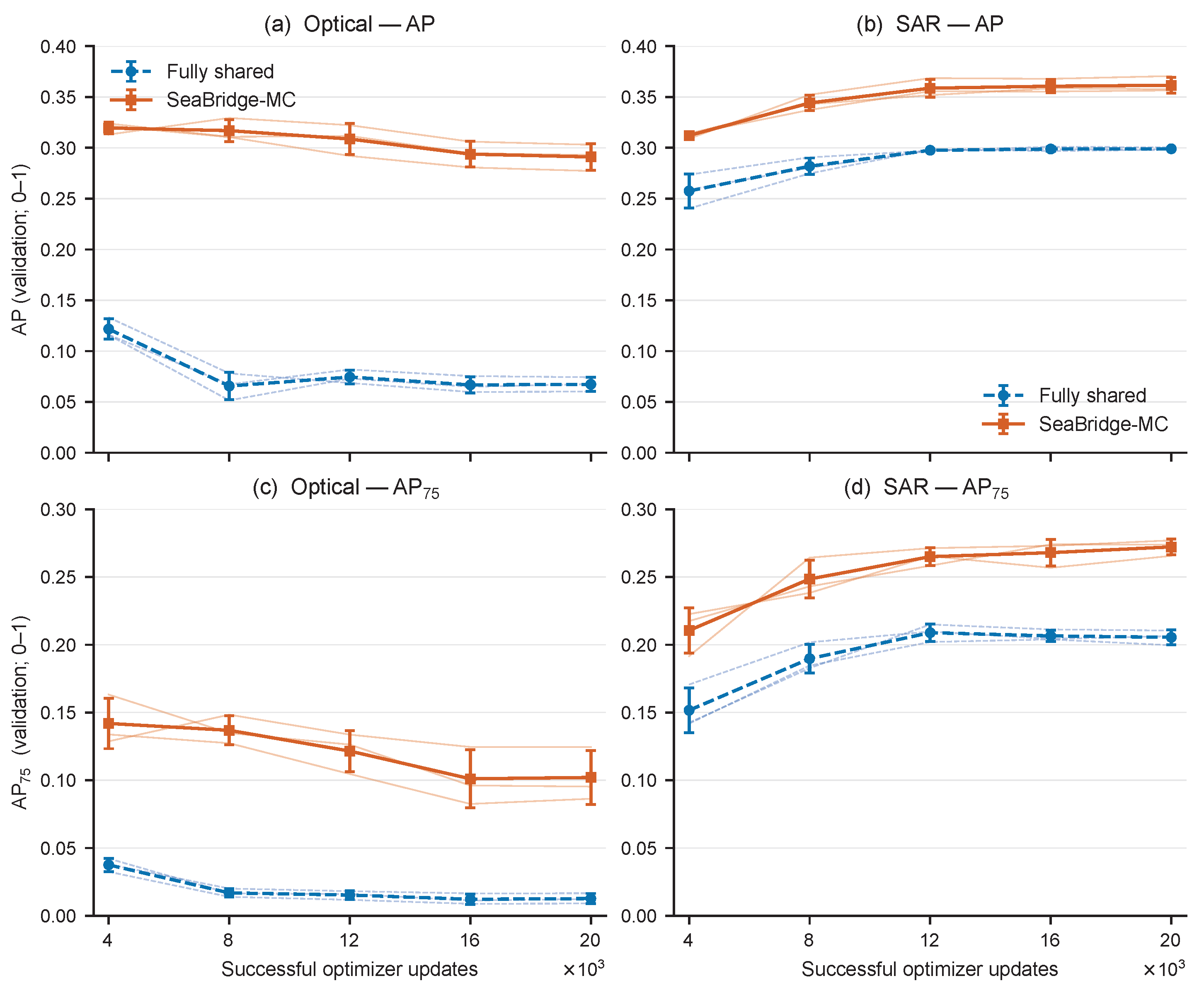
Decreasing training loss accompanied opposing validation trends in the additional optical-first runs over three common seeds (Figure 5 and Figure 6). Both models’ losses decreased in both domains, while optical validation AP and declined after early checkpoints and SAR AP generally increased under the same joint training budget.
Figure 5.
Domain training losses in the additional optical-first runs. Panels show the fully shared and SeaBridge-MC optical and SAR losses over seeds. Curves show mean criterion loss before the joint domain weight, using nonoverlapping 100-update bins; bands denote sample SD across seed-wise bin means. Thin lines show individual-seed trajectories. Insets enlarge updates 10,000–20,000 within the dotted boxes, with optical and SAR loss ranges of 4.5–6.5 and 6.5–8.5, respectively. Inset annotations give the horizontal (x) and vertical (y) magnification of distance per data unit relative to the corresponding main axes.
Figure 6.
Validation AP and in the same additional optical-first runs. Points show means over seeds at updates 4000, 8000, 12,000, 16,000, and 20,000; error bars show sample SD. Scores use the 0–1 scale. Thin lines show individual-seed trajectories.
Checkpoint selection shifted the optical–SAR balance while preserving SeaBridge-MC’s higher mean AP in both domains in the primary five-seed runs. Its test optical/SAR AP was 0.2451/0.4482 under selection, 0.2537/0.4318 under optical-AP selection, and 0.2279/0.4641 under SAR-AP selection. Each rule selected a single checkpoint for both domains.
4.4. Contributions of the Private Interfaces
Combining the private interfaces produced higher mean AP than either interface alone (Table 7). The optical and SAR gains were 0.0706 and 0.0305 over the private-stem model and 0.0776 and 0.0457 over the private-residual-BN model; the corresponding mean gains were and . The individual interfaces differed in consistency: private stems improved AP in both domains in every common seed, whereas private residual-stage normalization consistently improved optical AP and had seed-dependent effects on SAR AP.
Table 7.
Component and shared-capacity controls. Test AP is reported as mean ± sample SD over matched training seeds ( 2001–2003 ) on the 0–1 scale. The private-stem and private-residual-BN variants isolate the two components; the shared-capacity branch matches SeaBridge-MC’s parameter increment.
The parameter-matched shared branch remained close to the fully shared model at the tested insertion point, topology, and initialization. Its optical and SAR AP were 0.0525 and 0.3734, compared with 0.2382 and 0.4513 for SeaBridge-MC. Its mean paired difference from the fully shared model was , while SeaBridge-MC exceeded the shared-capacity model by .
4.5. Forward Order and Normalization Settings
The relative optical AP and of the two architectures depended on the BN setting (Table 8). SeaBridge-MC had higher mean AP in both domains under all three forward orders with updated running statistics. Fixed running statistics favored the fully shared model in optical AP and , while SeaBridge-MC retained higher mean SAR AP. Both architectures used the same training platform within each condition.
Table 8.
Additional test accuracy under forward-order and BN controls. Entries are mean ± sample SD over common seeds, on the 0–1 scale. Fixed denotes fixed running mean/variance with trainable affine parameters. All other rows update BN statistics.
4.6. Comparison with Independent Detectors
SeaBridge-MC supported both modalities with 49.90% fewer parameters than two independent detectors, at lower AP in each domain (Table 9). The joint detector used 20,121,396 parameters, compared with 40,166,056 for the independent pair. In the same-platform comparison over three common seeds, the AP differences (SeaBridge-MC minus independent training) were for optical imagery and for SAR imagery.
Table 9.
Independent and joint training in the additional experiments. Entries are mean ± sample SD on the 0–1 scale. The common-seed rows use seeds 2001–2003; the five-seed independent row additionally includes seeds 2004–2005. All systems were evaluated on the RTX 5080 Laptop GPU in FP32. Parameter counts include the complete joint model or both independent detectors.
4.7. Accuracy–Efficiency Trade-Off
SeaBridge-MC added 38,368 trainable parameters (0.1910%) and 0.184 MiB of logical state storage. Only one private branch was active for each input, and the counted computation remained 94.307 GFLOPs, with the remaining modules shared between domains (Table 10).
Table 10.
Model size and GPU-forward latency. Measurements use an RTX 5080 Laptop GPU, FP32, batch size 1, and synthetic inputs: 50 warm-up and 300 timed forwards per route. Timing excludes preprocessing, transfer, and post-processing. State denotes logical tensor storage; GFLOPs count supported operations. and denote median and 95th-percentile latency.
Median forward latency increased by 3.729 ms for optical inputs and 1.405 ms for SAR inputs, corresponding to 11.1% and 4.0%, respectively, in the single-session benchmark. The measured latency was therefore higher despite the unchanged count of supported floating-point operations.
4.8. Qualitative Detection Results
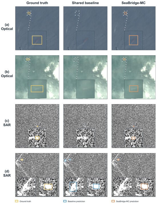
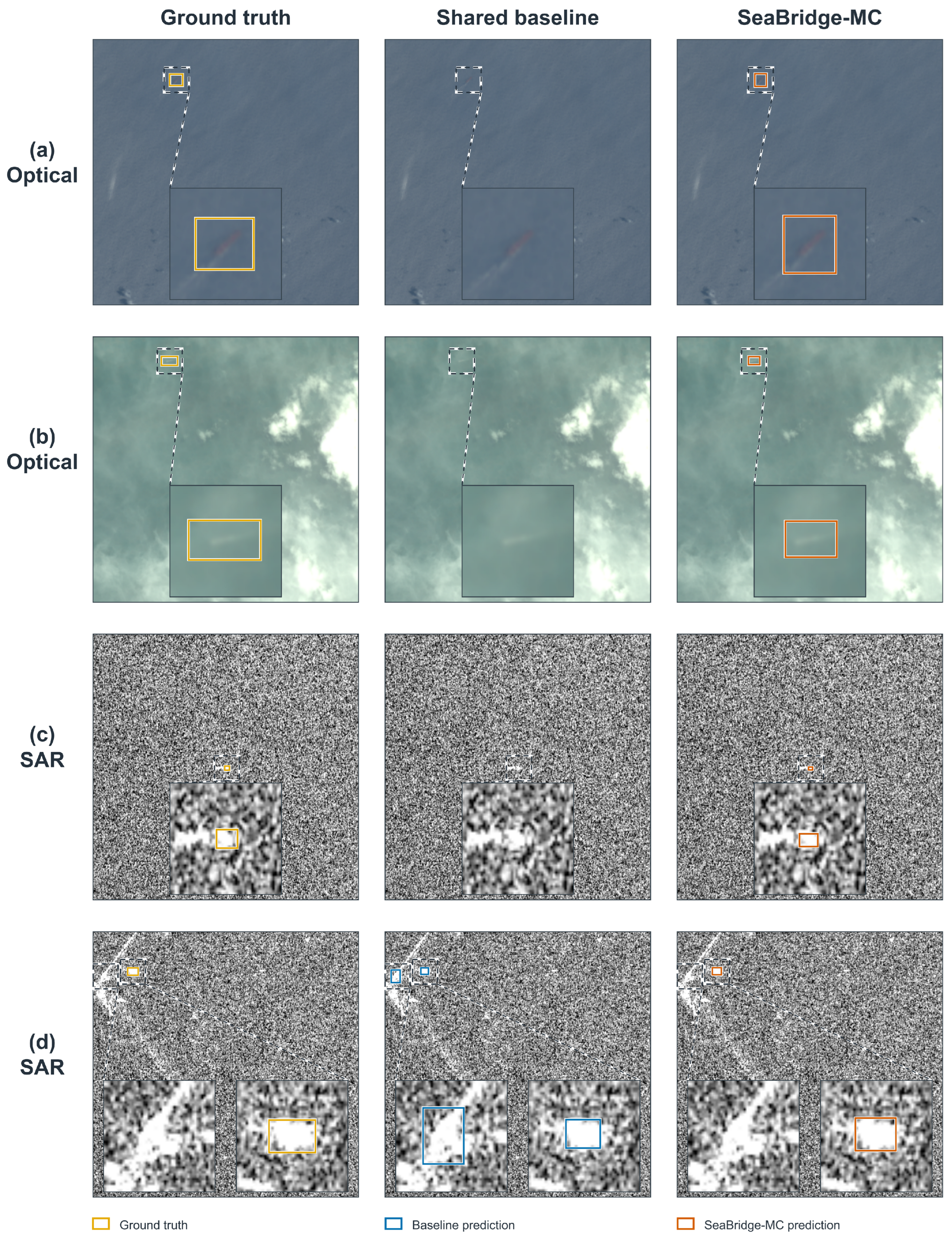
SeaBridge-MC recovered two low-contrast optical vessels missed by the fully shared model at the common display threshold (Figure 7). Image 1643 contained a faint elongated vessel among streak-like structures on a low-texture sea surface; image 69 contained a small ship under strongly nonuniform cloud and haze contamination. The recovered detections had IoUs of 0.8092 and 0.6480, respectively.
Figure 7.
Detections in challenging optical and SAR scenes. Rows (a–d) show optical images 1643 and 69 and SAR images 6723 and 791. Columns show ground truth (gold), the fully shared model (blue), and SeaBridge-MC (vermilion). Both models use validation-selected seed-2001 checkpoints and display predictions with scores . Dashed rectangles identify corresponding -pixel regions at a common magnification.
The SAR cases involved dense speckle, a tiny target, and structured clutter. In image 6723, SeaBridge-MC detected the annotated ship occupying native pixels amid dense speckle. Image 791 contained dense speckle and bright, spatially structured scatterers near the image boundary; SeaBridge-MC detected the annotated ship, avoided the fully shared model’s additional unmatched response, and increased matched-box IoU from 0.6354 to 0.7839.
4.9. Spatial Responses and Shared-Feature Discriminability
Assigned-query scores were higher for SeaBridge-MC in both attribution examples, while the changes in box IoU differed (Figure 8). In the optical example, the score increased from 0.458 to 0.814 and IoU increased from 0.235 to 0.342, remaining below 0.50. The fully shared model had a strong horizontal background response, whereas SeaBridge-MC showed attribution around the target and other image regions. In the SAR example, both maps include d responses near the ship and adjacent bright structures; SeaBridge-MC had the higher score (0.821 versus 0.664), while the fully shared model had the higher IoU (0.896 versus 0.772).
Figure 8.
Spatial attribution, response contrast, and gradient alignment. (a) Stage 3 Grad-CAM for optical image 884 and SAR image 7219, using seed-2001 validation-selected checkpoints. Cyan boxes mark the same annotated ship; outlined windows locate the -pixel source-image crops. Each map is computed from the raw ship logit of the ground-truth-assigned query and normalized by its full-image maximum; score and IoU refer to that query. (b) Stage 3 foreground–background feature-RMS ratios on 64 validation images per modality at validation-selected checkpoints. (c) Shared-convolution gradient cosine at the common 20,000-update endpoints. Paired points denote five detector seeds; summary marks show mean ± sample SD.
Foreground–background response contrast changed with both domain and feature depth. On the fixed subset of 64 images per modality, the optical Stage 3 ship–background RMS ratio increased from to across five seeds, with a positive paired change in every seed, while the SAR ratio decreased from to . Stage 4 ratios remained near unity, changing from 1.0236 to 1.0367 for optical inputs and from 0.9649 to 0.9500 for SAR inputs, with mixed seed-level directions.
Logistic probes of the unreduced ROI descriptors showed improved optical ship–background discriminability at both stages, with a mixed pattern for SAR. Optical AUROC increased from to at Stage 3 and from to at Stage 4; Stage 4 balanced accuracy increased from 0.8234 to 0.9719. SAR AUROC increased from to at Stage 3 and decreased slightly from to at Stage 4. The optical Stage 4 gain persisted under within-fold aggregation with equal and ROI-count weights, with paired differences of 0.0621 and 0.0778. The corresponding SAR differences averaged and , with scene-dependent directions.
4.10. Local Cross-Modal Gradient Geometry
Gradient alignment varied by stage and checkpoint. At the validation-selected checkpoints, Stage 3 mean cosine changed from for the fully shared model to for SeaBridge-MC; the fraction of negative batch-level cosines decreased from 56.25% to 48.75%. At Stage 4, mean cosine changed from to , and the negative fraction increased from 48.75% to 57.50%.
The common 20,000-update endpoints also showed heterogeneous local gradient relations (Figure 8c). Both models had mean cosine close to zero; the paired difference (SeaBridge-MC minus the fully shared model) was at Stage 3 and at Stage 4, with mixed directions across seeds. Negative-cosine frequency was identical at Stage 3 (51.25%) and lower for SeaBridge-MC at Stage 4 (42.50% versus 50.00%). Together with the selected-checkpoint results, these measurements showed stage- and checkpoint-dependent changes, with no uniform reduction in directional gradient conflict.
5. Discussion
Private input stems and residual-stage normalization improved the balance of a shared optical–SAR detector with BN running statistics updated during training. Relative to the fully shared model, the optical gain of 18.96 AP points, together with the SAR gain of 7.01 AP points, narrowed the absolute cross-dataset AP gap by 37.0%.
The component evidence is consistent with complementary roles for input and residual-stage specialization at the tested locations. The private-stem model achieved higher mean AP than private residual-stage BN, whose SAR effect varied across seeds, and combining the interfaces improved both domains further in the comparison over three common seeds. The tested parameter-matched shared branch remained close to the fully shared reference, supporting the private allocation over this particular shared expansion.
Optical reflectance, color, texture, and illumination-dependent contrast differ from the coherent backscatter, acquisition geometry, and speckle reflected in SAR amplitude [3,19]. These image-formation differences motivate modality-dependent input transformations, while the normalization controls establish the dependence of their accuracy benefit on the handling of BN running statistics. SeaBridge-MC had higher AP in both domains under all three forward orders with updated running statistics; fixed statistics favored the fully shared detector in optical AP and .
Optical feature discrimination improved at both measured stages, while response contrast changed with depth and modality. SeaBridge-MC had higher optical ship–background discriminability at Stages 3 and 4, with a smaller decline in AUROC between stages than the fully shared model. Optical foreground–background response contrast was stronger at Stage 3, whereas Stage 4 RMS ratios remained near unity. The slight decrease in SAR Stage 4 AUROC further distinguished the optical and SAR representational changes.
SeaBridge-MC exhibited a smaller decline in joint performance during continued training. Between the validation-selected checkpoint and update 20,000, both models lost optical AP and gained SAR AP, but the harmonic-mean decrease was almost five times as large for the fully shared model. SeaBridge-MC separates the scale, offset, running mean, and running variance for the optical and SAR branches while retaining shared residual convolutions [11]; the fully shared model uses one set of affine parameters and running moments in every residual-stage BN layer. The separate transformations act between shared convolutions and give branch-specific BN Jacobians in the frozen diagnostic.
The first-order loss change along the unpreconditioned joint direction depends on both gradient alignment and gradient magnitude. Endpoint cosines were close to zero, and changes across stages and checkpoints were small relative to between-seed variation and varied in sign. For a measured block l, the raw, unpreconditioned equal-weight direction has directional derivative for domain m. Thus, yields first-order ascent along this direction only if , where denotes the other domain [55]. This identity concerns the raw final-decoder gradients at the evaluated EMA state. Training combined the final-decoder, auxiliary, and denoising losses from both domains at every optimizer step, followed by global clipping and AdamW moment preconditioning. The finite-step response also depends on weight decay, learning rate, and local curvature.
The optical results distinguish strict-overlap localization from validation behavior during continued training on this tiny-ship dataset [1]. The large – difference persisted under both joint and independent training. In the matching analysis, the independent detector recovered more ground-truth boxes while giving similar median IoU among matched boxes. Optical validation AP and also declined after early checkpoints despite decreasing training loss.
The accuracy–parameter trade-off concerns the combined model required to support both modalities. SeaBridge-MC used 49.90% fewer parameters and 77.10 MiB of logical model state, compared with 153.84 MiB for the independent pair, with lower AP in both domains in the comparison over three common seeds. The fully shared model with fixed BN statistics used fewer parameters and achieved higher optical AP and harmonic-mean AP under that setting. In the separate GPU-forward benchmark, SeaBridge-MC had longer forward latency than the fully shared model.
6. Conclusions
SeaBridge-MC combines private input stems and residual-stage BN with a shared detection pathway for unpaired optical–SAR ship detection. Across five matched seeds with BN running statistics updated during training, it increased AP in both domains relative to the fully shared reference and reduced the absolute cross-dataset AP gap by 37.0%, with 38,368 additional trainable parameters. The component comparisons favored combining the interfaces over either alone and the tested shared-capacity branch. Fixed BN statistics reversed the optical AP and harmonic-mean AP ordering in favour of the fully shared model. In the separate comparison over three common seeds, SeaBridge-MC supported both modalities using approximately half the total parameters, with lower AP in each domain than the independent detectors.
Author Contributions
Conceptualization, G.M.; methodology, G.M.; software, S.Z.; validation, S.Z. and G.M.; formal analysis, S.Z.; investigation, S.Z.; resources, G.M.; data curation, S.Z.; writing—original draft preparation, S.Z.; writing—review and editing, G.M.; visualization, S.Z.; supervision, G.M.; project administration, G.M. All authors have read and agreed to the published version of the manuscript.
Funding
This research received no external funding.
Institutional Review Board Statement
Not applicable.
Informed Consent Statement
Not applicable.
Data Availability Statement
The LEVIR-Ship and OSSDD datasets analysed in this study are publicly available at [1,51]. The official repositories are available at https://github.com/WindVChen/LEVIR-Ship and https://huggingface.co/datasets/sylviaHoch/OpenSARShip-Ship-Detection-Dataset, respectively (accessed on 29 September 2026). The derived split manifests, resolved training configurations, per-seed results, selected-checkpoint identifiers, source code, and trained models are available from the corresponding author upon reasonable request.
Acknowledgments
We thank the contributors to the open-source datasets used in this study.
Conflicts of Interest
The authors declare no conflicts of interest.
References
- Chen, J.; Chen, K.; Chen, H.; Zou, Z.; Shi, Z. A Degraded Reconstruction Enhancement-Based Method for Tiny Ship Detection in Remote Sensing Images with a New Large-Scale Dataset. IEEE Trans. Geosci. Remote Sens. 2022, 60, 1–14. [Google Scholar] [CrossRef] [Scilit]
- Huang, L.; Liu, B.; Li, B.; Guo, W.; Yu, W.; Zhang, Z.; Yu, W. OpenSARShip: A Dataset Dedicated to Sentinel-1 Ship Interpretation. IEEE J. Sel. Top. Appl. Earth Obs. Remote Sens. 2018, 11, 195–208. [Google Scholar] [CrossRef] [Scilit]
- Li, J.; Xu, C.; Su, H.; Gao, L.; Wang, T. Deep Learning for SAR Ship Detection: Past, Present and Future. Remote Sens. 2022, 14, 2712. [Google Scholar] [CrossRef] [Scilit]
- Ding, J.; Xue, N.; Long, Y.; Xia, G.-S.; Lu, Q. Learning RoI Transformer for Oriented Object Detection in Aerial Images. In Proceedings of the IEEE/CVF Conference on Computer Vision and Pattern Recognition; IEEE: New York, NY, USA, 2019; pp. 2844–2853. [Google Scholar] [CrossRef] [Scilit]
- Han, J.; Ding, J.; Li, J.; Xia, G.-S. Align Deep Features for Oriented Object Detection. IEEE Trans. Geosci. Remote Sens. 2022, 60, 1–11. [Google Scholar] [CrossRef] [Scilit]
- Huang, M.; Xu, Y.; Qian, L.; Shi, W.; Zhang, Y.; Bao, W.; Wang, N.; Liu, X.; Xiang, X. A Bridge Neural Network-Based Optical-SAR Image Joint Intelligent Interpretation Framework. Space Sci. Technol. 2021, 2021, 9841456. [Google Scholar] [CrossRef] [Scilit]
- Zhang, W.; Zhang, X.; Xu, X.; Wei, S.; Shi, J.; Wang, Y.; Zeng, T. MHFNet: Multimodal Hybrid Fusion Framework for Misaligned SAR-Optical Ship Detection. ISPRS J. Photogramm. Remote Sens. 2026, 231, 151–166. [Google Scholar] [CrossRef] [Scilit]
- Luo, C.; Zhang, Y.; Guo, J.; Hu, Y.; Zhou, G.; You, H.; Ning, X. SAR-CDSS: A Semi-Supervised Cross-Domain Object Detection from Optical to SAR Domain. Remote Sens. 2024, 16, 940. [Google Scholar] [CrossRef] [Scilit]
- Zhao, S.; Luo, Y.; Zhang, T.; Guo, W.; Zhang, Z. A Domain Specific Knowledge Extraction Transformer Method for Multisource Satellite-Borne SAR Images Ship Detection. ISPRS J. Photogramm. Remote Sens. 2023, 198, 16–29. [Google Scholar] [CrossRef] [Scilit]
- Liu, S.; Li, D.; Song, H.; Fan, C.; Li, K.; Wan, J.; Liu, R. SAR Ship Detection across Different Spaceborne Platforms with Confusion-Corrected Self-Training and Region-Aware Alignment Framework. ISPRS J. Photogramm. Remote Sens. 2025, 228, 305–322. [Google Scholar] [CrossRef] [Scilit]
- Chang, W.-G.; You, T.; Seo, S.; Kwak, S.; Han, B. Domain-Specific Batch Normalization for Unsupervised Domain Adaptation. In Proceedings of the IEEE/CVF Conference on Computer Vision and Pattern Recognition, Long Beach, CA, USA, 15–20 June 2019; IEEE: New York, NY, USA, 2019; pp. 7346–7354. [Google Scholar] [CrossRef] [Scilit]
- Rebuffi, S.-A.; Bilen, H.; Vedaldi, A. Learning Multiple Visual Domains with Residual Adapters. arXiv 2017, arXiv:1705.08045. Available online: https://www.semanticscholar.org/paper/Learning-multiple-visual-domains-with-residual-Rebuffi-Bilen/d89ee98810039d2061ed42ee8026da49c503d16b (accessed on 3 November 2026).
- Chen, J.; Li, W.; Li, H.; Zhang, J. Deep Class-Specific Affinity-Guided Convolutional Network for Multimodal Unpaired Image Segmentation. In Medical Image Computing and Computer Assisted Intervention–MICCAI 2020; Lecture Notes in Computer Science; Springer: Cham, Switzerland, 2020; Volume 12264, pp. 187–196. [Google Scholar] [CrossRef] [Scilit]
- Li, Y.; Li, X.; Li, Y.; Zhang, Y.; Dai, Y.; Hou, Q.; Cheng, M.-M.; Yang, J. SM3Det: A Unified Model for Multi-Modal Remote Sensing Object Detection. Proc. AAAI Conf. Artif. Intell. 2026, 40, 6717–6725. [Google Scholar] [CrossRef] [Scilit]
- Hua, H.; Xu, W.; Liu, K.; Li, X.; Lu, J.; Li, D. Unpaired Cross-Modal Contrastive Learning for Dual-Modality Ship Detection. In 2026 Joint International Conference on Automation-Intelligence-Safety (ICAIS) and International Symposium on Autonomous Systems (ISAS); IEEE: New York, NY, USA, 2026; pp. 1–6. [Google Scholar] [CrossRef] [Scilit]
- Zou, Z.; Chen, K.; Shi, Z.; Guo, Y.; Ye, J. Object Detection in 20 Years: A Survey. Proc. IEEE 2023, 111, 257–276. [Google Scholar] [CrossRef] [Scilit]
- Lin, T.-Y.; Dollár, P.; Girshick, R.; He, K.; Hariharan, B.; Belongie, S. Feature Pyramid Networks for Object Detection. In Proceedings of the IEEE Conference on Computer Vision and Pattern Recognition; IEEE: New York, NY, USA, 2017; pp. 936–944. [Google Scholar] [CrossRef] [Scilit]
- Lin, T.-Y.; Goyal, P.; Girshick, R.; He, K.; Dollár, P. Focal Loss for Dense Object Detection. IEEE Trans. Pattern Anal. Mach. Intell. 2020, 42, 318–327. [Google Scholar] [CrossRef] [Scilit]
- Li, K.; Wan, G.; Cheng, G.; Meng, L.; Han, J. Object detection in optical remote sensing images: A survey and a new benchmark. ISPRS J. Photogramm. Remote Sens. 2020, 159, 296–307. [Google Scholar] [CrossRef] [Scilit]
- Ma, B.; Yang, H.; Yang, J. Ship Detection in Spaceborne SAR Images under Radio Interference Environment Based on CFAR. Electronics 2022, 11, 4135. [Google Scholar] [CrossRef] [Scilit]
- Sun, S.; Wang, J. Ship Detection in SAR Images Based on Steady CFAR Detector and Knowledge-Oriented GBDT Classifier. Electronics 2024, 13, 2692. [Google Scholar] [CrossRef] [Scilit]
- Xia, R.; Chen, J.; Huang, Z.; Wan, H.; Wu, B.; Sun, L.; Yao, B.; Xiang, H.; Xing, M. CRTransSar: A Visual Transformer Based on Contextual Joint Representation Learning for SAR Ship Detection. Remote Sens. 2022, 14, 1488. [Google Scholar] [CrossRef] [Scilit]
- Zheng, H.; Xue, X.; Yue, R.; Liu, C.; Liu, Z. SAR Image Ship Target Detection Based on Receptive Field Enhancement Module and Cross-Layer Feature Fusion. Electronics 2024, 13, 167. [Google Scholar] [CrossRef] [Scilit]
- Wang, S.; Min, B.-W.; Li, G.; Gao, D.; Qiu, J.; Hong, Y. S2D-Net: A Synergistic Star-Attentive Network with Dynamic Feature Refinement for Robust Inshore SAR Ship Detection. Electronics 2026, 15, 1160. [Google Scholar] [CrossRef] [Scilit]
- Li, K.; Wang, D.; Hu, Z.; Zhu, W.; Li, S.; Wang, Q. Unleashing Channel Potential: Space-Frequency Selection Convolution for SAR Object Detection. In Proceedings of the IEEE/CVF Conference on Computer Vision and Pattern Recognition; IEEE: New York, NY, USA, 2024; pp. 17323–17332. [Google Scholar] [CrossRef] [Scilit]
- Zhang, Z.; Zhang, L.; Wang, Y.; Feng, P.; He, R. ShipRSImageNet: A Large-Scale Fine-Grained Dataset for Ship Detection in High-Resolution Optical Remote Sensing Images. IEEE J. Sel. Top. Appl. Earth Obs. Remote Sens. 2021, 14, 8458–8472. [Google Scholar] [CrossRef] [Scilit]
- Wei, S.; Zeng, X.; Qu, Q.; Wang, M.; Su, H.; Shi, J. HRSID: A High-Resolution SAR Images Dataset for Ship Detection and Instance Segmentation. IEEE Access 2020, 8, 120234–120254. [Google Scholar] [CrossRef] [Scilit]
- Fuller, A.; Millard, K.; Green, J.R. CROMA: Remote Sensing Representations with Contrastive Radar-Optical Masked Autoencoders. In Advances in Neural Information Processing Systems; Curran Associates, Inc.: Red Hook, NY, USA, 2023; Volume 36, pp. 5506–5538. [Google Scholar] [CrossRef] [Scilit]
- Zhang, Y.; Ru, L.; Wu, K.; Yu, L.; Liang, L.; Li, Y.; Chen, J. SkySense V2: A Unified Foundation Model for Multi-Modal Remote Sensing. In Proceedings of the IEEE/CVF International Conference on Computer Vision; IEEE: New York, NY, USA, 2025; pp. 9136–9146. [Google Scholar] [CrossRef] [Scilit]
- Zhang, J.; Lei, J.; Xie, W.; Fang, Z.; Li, Y.; Du, Q. SuperYOLO: Super Resolution Assisted Object Detection in Multimodal Remote Sensing Imagery. IEEE Trans. Geosci. Remote Sens. 2023, 61, 1–15. [Google Scholar] [CrossRef] [Scilit]
- Zhang, L.; Jiang, Y.; Yang, W.; Liu, B. SGFNet: Semantic-Guided Fusion Network with Closed-Loop Feedback for RGB–Infrared Oriented Object Detection. Electronics 2026, 15, 1003. [Google Scholar] [CrossRef] [Scilit]
- Hu, Q.; Yu, H.; Zhou, Z.; Li, S. IAF-RTDETR: Illumination Evaluation-Driven Multimodal Object Detection Network for Infrared–Visible Dual-Source Fusion. Electronics 2026, 15, 1332. [Google Scholar] [CrossRef] [Scilit]
- Chen, Y.; Li, W.; Sakaridis, C.; Dai, D.; Van Gool, L. Domain Adaptive Faster R-CNN for Object Detection in the Wild. In Proceedings of the IEEE/CVF Conference on Computer Vision and Pattern Recognition; IEEE: New York, NY, USA, 2018; pp. 3339–3348. [Google Scholar] [CrossRef] [Scilit]
- Zhang, M.; Sun, J.; Wang, H. Ship Detection in SAR Images via Source-Free Domain Adaptation From Optical Image Domain. IEEE Geosci. Remote Sens. Lett. 2025, 22, 1–5. [Google Scholar] [CrossRef] [Scilit]
- Wu, B.; Wang, H.; Zhang, C.; Chen, J. Optical-to-SAR Translation Based on CDA-GAN for High-Quality Training Sample Generation for Ship Detection in SAR Amplitude Images. Remote Sens. 2024, 16, 3001. [Google Scholar] [CrossRef] [Scilit]
- Wang, S.; Huang, Y.; Wang, P.; Lu, L.; Huang, H. Optical-to-SAR Domain Adaptation with Inversion Regularization for Unsupervised Ship Detection. Knowl.-Based Syst. 2026, 334, 115044. [Google Scholar] [CrossRef] [Scilit]
- Ran, L.; Li, J.; Wu, H.; Wu, A.; He, Y.; Guan, Q.; Zhu, Q. Bridging Optical and SAR Images via Semantic Prompt-Guided Progressive Alignment for Rotated Cross-Domain Ship Detection. Int. J. Appl. Earth Obs. Geoinf. 2026, 146, 105119. [Google Scholar] [CrossRef] [Scilit]
- Misra, I.; Shrivastava, A.; Gupta, A.; Hebert, M. Cross-Stitch Networks for Multi-task Learning. In Proceedings of the IEEE Conference on Computer Vision and Pattern Recognition, Las Vegas, NV, USA; IEEE: New York, NY, USA, 2016; pp. 3994–4003. [Google Scholar] [CrossRef] [Scilit]
- Wang, Y.; Sun, F.; Lu, M.; Yao, A. Learning Deep Multimodal Feature Representation with Asymmetric Multi-layer Fusion. In Proceedings of the 28th ACM International Conference on Multimedia; ACM: New York, NY, USA, 2020; pp. 3902–3910. [Google Scholar] [CrossRef] [Scilit]
- Han, B.; Zhang, S.; Shi, X.; Reichstein, M. Bridging Remote Sensors with Multisensor Geospatial Foundation Models. In Proceedings of the IEEE/CVF Conference on Computer Vision and Pattern Recognition; IEEE: New York, NY, USA, 2024; pp. 27852–27862. [Google Scholar] [CrossRef] [Scilit]
- Li, Y.; Li, X.; Li, W.; Hou, Q.; Liu, L.; Cheng, M.-M.; Yang, J. SARDet-100K: Towards Open-Source Benchmark and ToolKit for Large-Scale SAR Object Detection. In Advances in Neural Information Processing Systems; Curran Associates, Inc.: Red Hook, NY, USA, 2024; Volume 37, pp. 128430–128461. [Google Scholar] [CrossRef] [Scilit]
- Zhao, Y.; Lv, W.; Xu, S.; Wei, J.; Wang, G.; Dang, Q.; Liu, Y.; Chen, J. DETRs Beat YOLOs on Real-Time Object Detection. In Proceedings of the IEEE/CVF Conference on Computer Vision and Pattern Recognition, Seattle, WA, USA; IEEE: New York, NY, USA, 2024; pp. 16965–16974. [Google Scholar] [CrossRef] [Scilit]
- Lv, W.; Zhao, Y.; Chang, Q.; Huang, K.; Wang, G.; Liu, Y. RT-DETRv2: Improved Baseline with Bag-of-Freebies for Real-Time Detection Transformer. arXiv 2024, arXiv:2407.17140. [Google Scholar] [CrossRef] [Scilit]
- He, K.; Zhang, X.; Ren, S.; Sun, J. Deep Residual Learning for Image Recognition. In Proceedings of the IEEE Conference on Computer Vision and Pattern Recognition; IEEE: New York, NY, USA, 2016; pp. 770–778. [Google Scholar] [CrossRef] [Scilit]
- He, T.; Zhang, Z.; Zhang, H.; Zhang, Z.; Xie, J.; Li, M. Bag of Tricks for Image Classification with Convolutional Neural Networks. In Proceedings of the IEEE/CVF Conference on Computer Vision and Pattern Recognition; IEEE: New York, NY, USA, 2019; pp. 558–567. [Google Scholar] [CrossRef] [Scilit]
- Carion, N.; Massa, F.; Synnaeve, G.; Usunier, N.; Kirillov, A.; Zagoruyko, S. End-to-End Object Detection with Transformers. In Computer Vision – ECCV 2020; Springer: Cham, Switzerland, 2020; pp. 213–229. [Google Scholar] [CrossRef] [Scilit]
- Zhu, X.; Su, W.; Lu, L.; Li, B.; Wang, X.; Dai, J. Deformable DETR: Deformable Transformers for End-to-End Object Detection. In Proceedings of the International Conference on Learning Representations, Virtual Conference, 3–7 May 2021; Available online: https://iclr.cc/virtual/2021/poster/3105 (accessed on 3 November 2026).
- Ioffe, S.; Szegedy, C. Batch Normalization: Accelerating Deep Network Training by Reducing Internal Covariate Shift. In Proceedings of the 32nd International Conference on Machine Learning; PMLR; Curran Associates, Inc.: Red Hook, NY, USA, 2015; Volume 37, pp. 448–456. Available online: https://proceedings.mlr.press/v37/ioffe15.html (accessed on 3 November 2026).
- Zhang, H.; Wang, Y.; Dayoub, F.; Sünderhauf, N. VarifocalNet: An IoU-aware Dense Object Detector. In Proceedings of the IEEE/CVF Conference on Computer Vision and Pattern Recognition; IEEE: New York, NY, USA, 2021; pp. 8510–8519. [Google Scholar] [CrossRef] [Scilit]
- Rezatofighi, H.; Tsoi, N.; Gwak, J.; Sadeghian, A.; Reid, I.; Savarese, S. Generalized Intersection Over Union: A Metric and a Loss for Bounding Box Regression. In Proceedings of the IEEE/CVF Conference on Computer Vision and Pattern Recognition; IEEE: New York, NY, USA, 2019; pp. 658–666. [Google Scholar] [CrossRef] [Scilit]
- Hammer, H.; Hochstuhl, S.; Thiele, A.; Brosch, T.; Davidson, P.; Remiger, T.; Teutsch, M. OSSDD–a New Open Dataset for Sentinel-1 Ship Detection. arXiv 2026, arXiv:2608.01963. [Google Scholar] [CrossRef] [Scilit]
- Loshchilov, I.; Hutter, F. Decoupled Weight Decay Regularization. In Proceedings of the International Conference on Learning Representations, New Orleans, LA, USA, 6–9 May 2019; Available online: https://iclr.cc/virtual/2019/poster/935 (accessed on 3 November 2026).
- Lin, T.-Y.; Maire, M.; Belongie, S.; Hays, J.; Perona, P.; Ramanan, D.; Dollár, P.; Zitnick, C.L. Microsoft COCO: Common Objects in Context. In Computer Vision–ECCV 2014; Springer: Cham, Switzerland, 2014; pp. 740–755. [Google Scholar] [CrossRef] [Scilit]
- Selvaraju, R.R.; Cogswell, M.; Das, A.; Vedantam, R.; Parikh, D.; Batra, D. Grad-CAM: Visual Explanations from Deep Networks via Gradient-Based Localization. In Proceedings of the IEEE International Conference on Computer Vision, Venice, Italy; IEEE: New York, NY, USA, 2017; pp. 618–626. [Google Scholar] [CrossRef] [Scilit]
- Yu, T.; Kumar, S.; Gupta, A.; Levine, S.; Hausman, K.; Finn, C. Gradient Surgery for Multi-Task Learning. In NIPS’20: 34th International Conference on Neural Information Processing Systems; Curran Associates, Inc.: Red Hook, NY, USA, 2020; Volume 33, pp. 5824–5836. Available online: https://dl.acm.org/doi/10.5555/3495724.3496213 (accessed on 3 November 2026).

Disclaimer/Publisher’s Note: The statements, opinions and data contained in all publications are solely those of the individual author(s) and contributor(s) and not of MDPI and/or the editor(s). MDPI and/or the editor(s) disclaim responsibility for any injury to people or property resulting from any ideas, methods, instructions or products referred to in the content. |
© 2026 by the authors. Licensee MDPI, Basel, Switzerland. This article is an open access article distributed under the terms and conditions of the Creative Commons Attribution (CC BY) license.