Temperature–Salinity Coupled Compensation for Conductance-Based Water-Cut Measurement Using a Bayesian-Regularized Backpropagation Neural Network

Abstract

Conductance-based water-cut measurements are sensitive to coupled changes in temperature and salinity. This study develops a Bayesian-regularized backpropagation neural network (BR-BPNN) for compensation using the mean sensor peak voltage, temperature, and salinity as inputs. A grid of 198 measured calibration points was used to construct a trilinear response surface and generate 9000 derived samples for developing BR-BPNN, a ridge-regularized nonlinear basis-expansion baseline (MPR), and support vector regression (SVR). On 40 independently measured test conditions spanning 55–95% nominal water cut, the fitted BR-BPNN achieved a mean absolute error of 1.72 percentage points, compared with 3.52 for MPR and 2.32 for SVR under the reported model-selection procedures. Training-strategy comparisons and physical-plane holdouts further assessed interpolation-based training. The selected 3-10-5-1 network was deployed on an STM32L496RGT3 and evaluated with newly acquired sensor inputs under the same 40 nominal conditions. Embedded evaluation achieved a mean absolute error of 1.868 percentage points and a mean network forward-inference time of 52.05 μs. The results demonstrate a compact implementation of coupled compensation for embedded conductance-based water-cut measurement within the tested laboratory domain.

1. Introduction

Water cut is a key parameter in oil–water two-phase flow. Accurate measurement supports water-breakthrough identification, reservoir monitoring, and injection-production optimization. Common measurement methods include capacitive, ultrasonic, microwave, and conductance-based techniques [1,2,3,4]. Conductance-based sensors exploit the electrical contrast between the oil and aqueous phases. Their fast response, simple structure, and ease of integration make them attractive for water-cut measurement [5,6].

The electrical response of an oil–water mixture depends on aqueous-phase conductivity and phase distribution as well as water cut. Salinity effects have also been investigated using microwave water-cut sensors [7]. For conductance probes, temperature changes ionic mobility, whereas salinity changes ion concentration and ion–ion interactions. Their coupled influence produces signal drift and nonlinear responses, particularly at high salinity and within the response-transition range.

Previous studies have improved conductance-based phase-fraction measurement through sensing-mechanism analysis, temperature compensation, and sensor design. Shi et al. [8] identified aqueous conductivity, flow structure, and sensor geometry as key influences on conductance measurements. Wiedemann et al. [9] demonstrated temperature compensation for conductivity-based phase-fraction measurements. Wang et al. [10] reported absolute water-holdup errors below 5% for a horizontal-well application, and Han et al. [11] reported accuracy better than 3.23% using phase-state regulation. These studies establish the potential of conductance sensing and motivate compensation that represents coupled fluid-property effects.

Physics-based models offer good interpretability and low computational cost. However, they usually rely on simplifying assumptions. Such assumptions can limit their ability to describe strong nonlinear coupling at high salinity and within the response-transition range. Their calibration accuracy and generalization performance may therefore deteriorate under these conditions.

Data-driven methods represent nonlinear inverse relationships without prescribing a fixed analytical form. Dai et al. [12] used Bayesian-optimized XGBoost for temperature–salinity correction and reported an average absolute error of 1.50% under their protocol. Yan et al. [13] reviewed soft-computing approaches to multiphase-flow measurement, while Zhang and Xia [14] combined RS-SVM and GA-NN for dielectric-based water-content estimation. Such methods provide flexible compensation models, while their structure and implementation determine the training requirements and online computational cost.

Existing approaches therefore involve a trade-off between interpretability, nonlinear representation, and computational cost. Mechanism-based models are efficient but may underrepresent strong coupling. Data-driven models can improve accuracy but may require greater computational resources. Achieving accurate multi-parameter compensation under embedded real-time constraints remains an important challenge for conductance-based water-cut measurement.

This study addresses this challenge through four contributions. First, a multi-condition experimental platform characterizes the sensor response over a measured temperature–salinity–water-cut grid. Second, MPR and SVR provide explicit-regression and nonlinear-kernel baselines using common inputs, normalization, and development data. Third, a compact BR-BPNN is developed and evaluated on 40 separately measured conditions, with training-strategy ablation and physical-plane holdouts assessing trilinear augmentation. Finally, the selected network is deployed on an STM32L496RGT3, and its prediction accuracy, forward-inference time, and firmware memory requirements are experimentally evaluated.

2. Measurement Principle and System Design

2.1. Principle of Conductance-Based Water-Cut Measurement

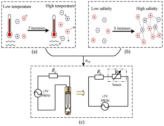
The sensing mechanism is considered at two levels: ionic conduction in the aqueous phase and the equivalent electrical response of the sensor interface. In an oil–water mixture, the oil phase is weakly conductive relative to the saline aqueous phase. The measured response therefore depends on aqueous-phase conductivity and on the connectivity of conductive water pathways. Temperature T, salinity S, and nominal water cut Y_w consequently produce coupled changes in the probe response. The influence of temperature and salinity on sensor response is illustrated in Figure 1.

Figure 1. Influence of temperature and salinity on sensor response: (a) temperature-dependent ionic mobility; (b) salinity-dependent ion concentration and interactions; (c) conductance-probe circuit illustration with a 10 kHz, ±5 V bipolar excitation (10 V peak to peak). Red and blue circles represent different types of ions, and dotted arrows indicate ionic mobility.

At the microscopic level, the aqueous-phase conductivity σ_w is governed by the concentration and mobility of ionic charge carriers and can be written in the conventional form

$${\sigma }_{\mathrm{w}}=F{\displaystyle \sum z_i}{u}_i{c}_i$$

(1)

where σ_w is the aqueous-phase electrical conductivity (S/m), F is the Faraday constant (96,485 C/mol), and z_i, u_i, and c_i denote the magnitude of ionic valence, ionic mobility (m²·V⁻¹·s⁻¹), and molar concentration (mol/m³) of species i, respectively.

Temperature alters ionic transport through changes in viscosity and mobility, while salinity changes charge-carrier concentration and, at high concentration, ion–ion interactions [15,16,17,18]. The aqueous conductivity is therefore represented as σ_w = σ_w(T,S). These mechanisms link the ionic response to the experimentally calibrated voltage and motivate joint temperature–salinity compensation.

At the mixture scale, nominal water cut changes the fraction and connectivity of the conductive aqueous phase within the weakly conductive oil phase. Under the controlled mixing conditions used here, the equivalent mixture conductivity can be approximated as

σ_eq = σ_eq(Y_w,T,S) ≈ σ_w(T,S)g(Y_w)

(2)

where σ_eq(Y_w,T,S) is the equivalent mixture conductivity (S/m), σ_w(T,S) is the intrinsic aqueous-phase conductivity (S/m), and g(Y_w) represents the dominant structural contribution of aqueous-phase fraction and conductive-path connectivity. Here, S is the NaCl mass concentration in the aqueous phase (mg/L).

Temperature and salinity can also affect viscosity, interfacial behavior, phase distribution, and conductive-path formation. The mixture response can therefore be expressed more generally as

σ_eq(Y_w,T,S) = σ_w(T,S)g(Y_w) + ε_c(Y_w,T,S)

(3)

where ε_c denotes the aggregate residual coupling associated with hydrodynamic and phase-distribution effects not captured by the first-order approximation.

At low nominal water cut, the conductive aqueous phase has limited connectivity and the equivalent mixture conductivity remains low. As water cut increases, conductive paths develop progressively. The mixture response then becomes more sensitive to the intrinsic aqueous conductivity σ_w(T,S).

This water-cut-dependent change in conductive connectivity provides a physical basis for the nonlinear response [19,20,21]. Its combined dependence on phase distribution and fluid properties is represented by calibration across the measured temperature–salinity–water-cut grid.

The fluid–electrode interface couples mixture conductivity to the sensing circuit and is represented by an effective resistance R_m in parallel with a lumped capacitance C_p. To first order, R_m decreases as mixture conductivity increases, approximately as R_m~K_c/σ_eq, where K_c is an effective cell constant associated with electrode geometry and phase distribution. The corresponding complex impedance is

$$Z_s=R_m\parallel {\displaystyle \frac{1}{\mathit{j\omega }{C}_p}}={\displaystyle \frac{R_m}{1+\mathit{j\omega }{R}_m{C}_p}}$$

(4)

where Z_s is the complex sensor impedance, R_m is the effective conductive resistance (Ω), and C_p is the lumped capacitance (F). The symbol j denotes the imaginary unit, and ω = 2πf is the angular excitation frequency. A fixed excitation frequency of 10 kHz is used in the experiments.

The sensor impedance Z_s and reference resistor R_d form a voltage divider. The single-frequency equivalent-circuit voltage-divider relation is written as

$$U_{\mathrm{out}}=U_{\mathrm{in}}{\displaystyle \frac{Z_s}{R_d+Z_s}}$$

(5)

where U_in and U_out are the complex excitation and sensor-branch voltages in the equivalent circuit, R_d = 51 kΩ. The voltage feature V is the average of the sensor output voltage peaks measured during the positive-excitation half-cycles.

Equations (2)–(5) link the mixture electrical properties to the measured voltage feature. Temperature and salinity modify the intrinsic aqueous conductivity, while water cut changes conductive-path connectivity. These effects alter the effective sensor impedance and the measured voltage amplitude. Thus, V cannot be treated as a function of water cut alone. The present system records only voltage amplitude at one excitation frequency. Consequently, R_m and C_p cannot be identified independently at each operating point. Their combined influence is retained in the measured feature V.

The combined circuit response is represented by the forward mapping V = H(Y_w,T,S). Water-cut compensation is formulated as the inverse mapping Y_w = G(V,T,S), using voltage together with temperature and salinity. This connects the sensing mechanism directly to the three-input compensation models in Section 4.

2.2. Measurement System Architecture

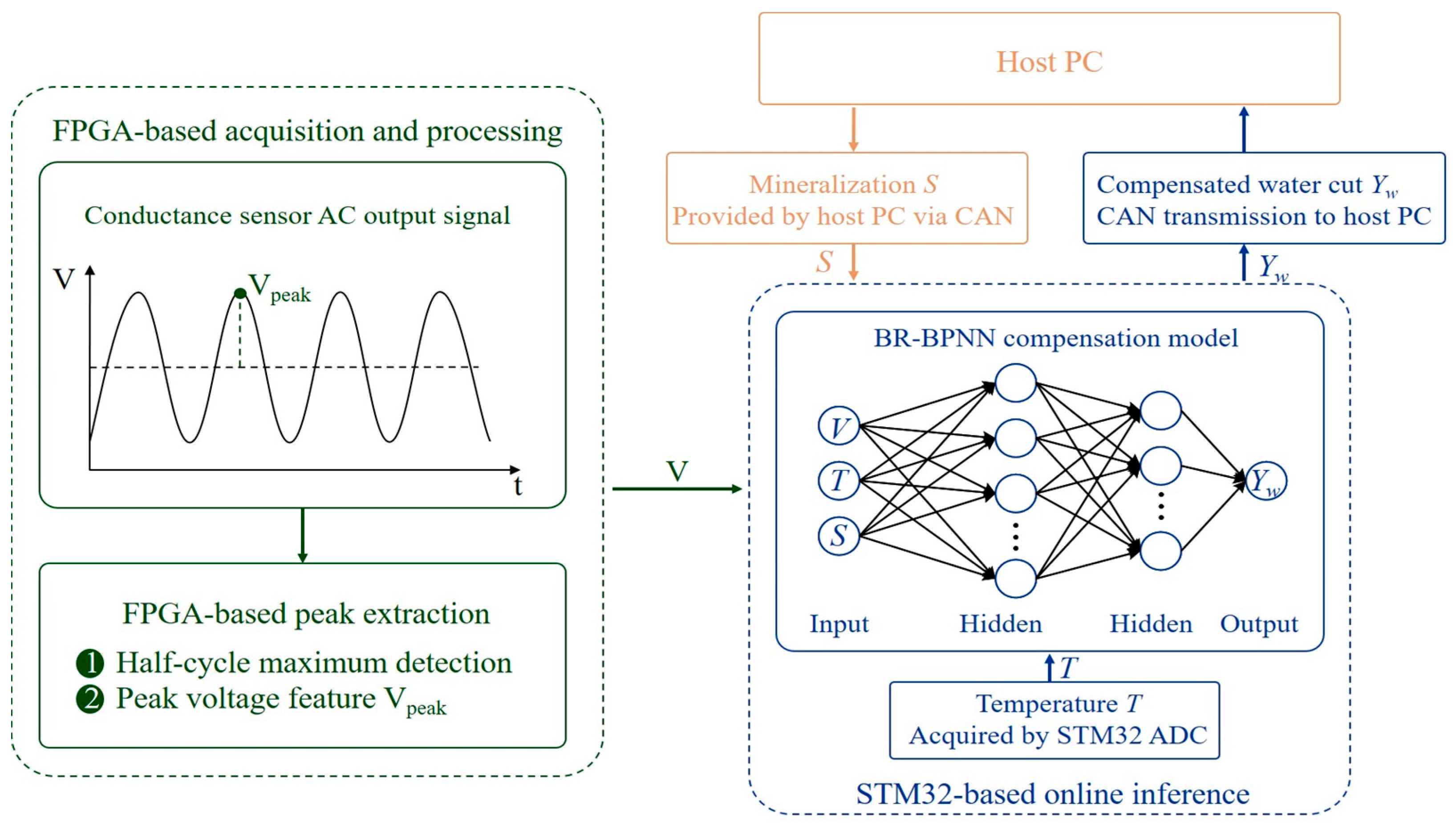
The prototype uses a heterogeneous architecture based on an STM32L496RGT3 microcontroller (STMicroelectronics, Geneva, Switzerland) and an A3P250-VQ100 FPGA (Microchip Technology Inc., Chandler, AZ, USA). The FPGA provides deterministic excitation and acquisition timing, controls ADS8665 (Texas Instruments, Dallas, TX, USA) sampling, and extracts the mean peak-voltage feature. The extracted voltage is transmitted to the STM32 through USART. The STM32 acquires temperature, receives the externally supplied salinity value, performs model inference, manages system operation, and communicates with the host computer through CAN. This partition assigns time-critical acquisition to the FPGA and compensation inference to the microcontroller.

A fixed 10 kHz bipolar excitation of ±5 V, corresponding to 10 V peak-to-peak, was used for calibration and testing. A precision resistor R_d = 51 kΩ forms a voltage divider with the probe impedance, and a 12-bit ADS8665 [22] digitizes the response under FPGA timing control. The FPGA extracts the mean sensor peak voltage V from the positive-excitation half-cycles, as described above. The acquisition-channel noise-and-quantization budget gives an estimated SNR of approximately 71.5 dB.

As shown in Figure 2, the host supplies control commands and the external salinity value S to the STM32 and receives the compensated water-cut estimate. In the experiments, S was the prescribed NaCl concentration of the prepared aqueous phase. In practical applications, the input can be obtained from produced-water sampling or a calibrated upstream aqueous-phase analyzer, with the value and acquisition timestamp supplied to the controller.

Figure 2. Schematic diagram of the conductance-based crude oil water-cut measurement system.

For a small salinity-input error at fixed V and T, the local prediction change is ΔY_w ≈ (∂G/∂S)ΔS. During a transient, an update delay τ gives ΔS(t) = S(t − τ) − S(t), so the resulting water-cut bias depends on both the salinity rate of change and the local model sensitivity. Timestamped updates or synchronized salinity measurements reduce this mismatch. Section 4.4.2 evaluates the static sensitivity numerically.

During measurement, the FPGA provides the voltage-amplitude feature V. The STM32 combines V with the measured temperature T and the supplied salinity S. Model training and parameter optimization are completed offline. The trained compensation model is then transferred to the STM32, where only forward inference is executed. Embedded accuracy, latency, and memory consumption are evaluated separately in Section 4.5.

3. Experimental Method and Sensor Response Analysis

3.1. Experimental Platform and Test Procedure

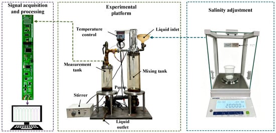
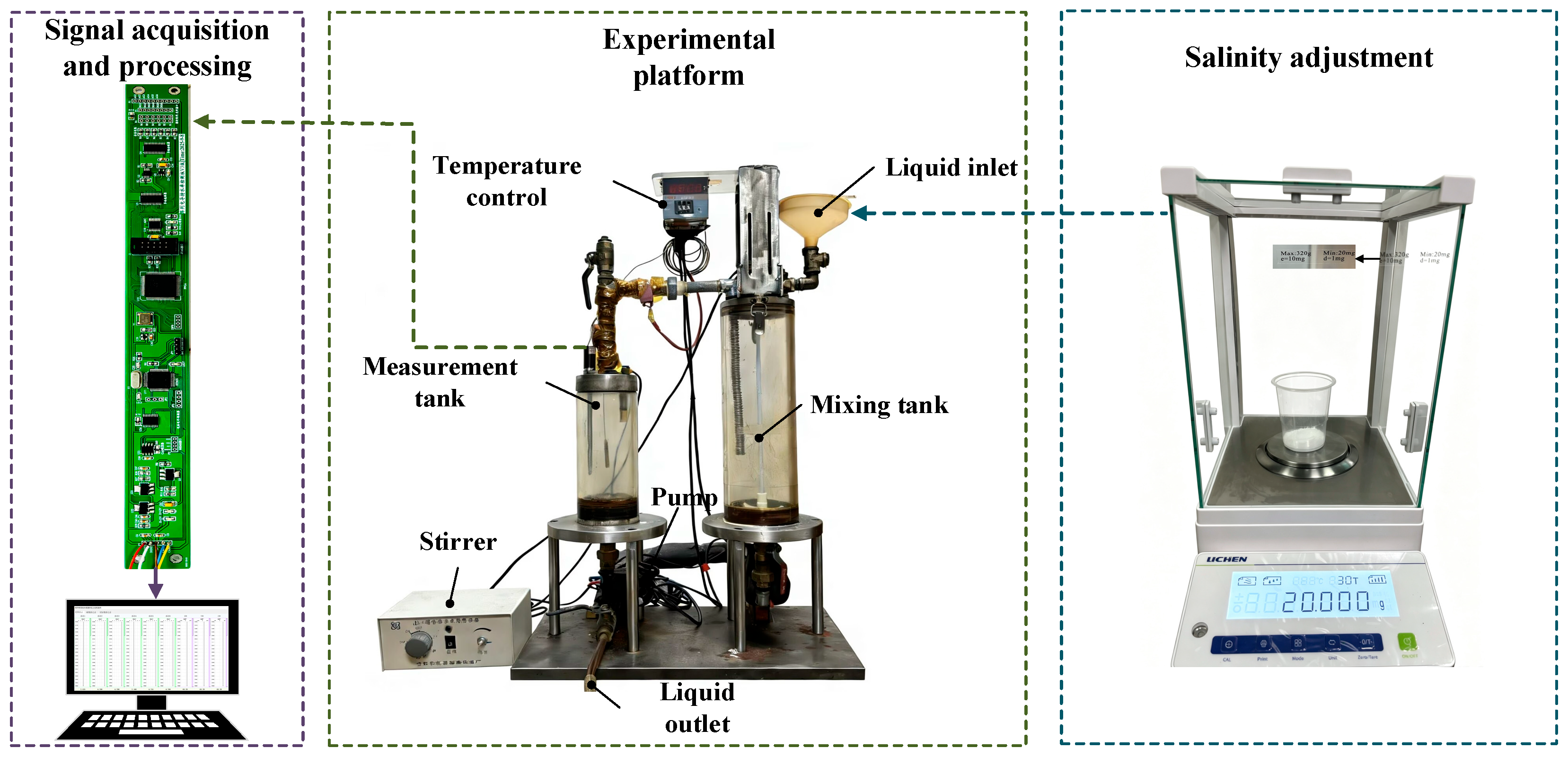
The laboratory mixing and recirculation platform in Figure 3 includes a mixing tank, measurement section, conductance probe, mechanical stirrer, temperature controller, and circulation pump. Diesel (Sinopec, Jingzhou, China) and NaCl (Huizhou Zhiwei Chemical Technology Co., Ltd., Huizhou, China) aqueous solutions served as the oil and aqueous phases. Calibration and independent testing used a total loop flow rate of 30 m³/d and a stirrer speed of 500 r/min.

Figure 3. Experimental platform for oil–water two-phase flow measurement.

Changes in field flow velocity can alter droplet dispersion, local phase distribution, and conductive-path connectivity near the electrodes [11,20,23,24,25]. Stratified or slug flow may therefore give a different local voltage at the same prepared volumetric water cut. The fixed circulation and stirring settings provide a common hydrodynamic basis for studying temperature–salinity coupling; extension to variable field flows requires calibration or validation across the relevant hydrodynamic range.

Reference water-cut values were established by volumetric preparation. Each mixture had a nominal total liquid volume of 3000 mL. Graduated cylinders with capacities of 100–3000 mL and minimum graduations of 1–20 mL were selected according to the required phase volume. The largest suitable cylinder was used where possible, and smaller cylinders were used for final adjustment. The prepared oil and aqueous phases were then mixed under the prescribed stirring condition before circulation and data acquisition.

The reference water cut, Y_w, is defined as the nominal volumetric water fraction:

$$Y_{\mathrm{w}}={\displaystyle \frac{V_{\mathrm{w}}}{V_{\mathrm{w}}+V_{\mathrm{o}}}}$$

(6)

where V_w and V_o denote the prepared aqueous and oil volumes, respectively. This nominal volumetric fraction is used as the reference water-cut value for both model calibration and independent evaluation.

For each operating point, the prepared mixture was circulated under the fixed stirring and flow conditions. Data acquisition began after the target temperature was reached and the sensor output stabilized. The voltage-amplitude feature was then recorded using the system described in Section 2.2. The measured voltage, temperature, and salinity were assigned either to model development or to independent evaluation according to the experimental design.

The calibration grid contains 198 physically measured operating points. The 40 blind-test conditions were acquired in a separate campaign using freshly prepared oil–water mixtures and directly recorded sensor voltages after temperature and signal stabilization. Reference water cuts were calculated from the separately prepared phase volumes. The test combinations differ from the calibration nodes and were excluded from response-surface construction, original model fitting, architecture selection, and hyperparameter tuning.

3.2. Sensor Response Characteristics

Experiments were conducted at three temperatures (25, 45, and 65 °C), six salinity levels (0, 5000, 10,000, 20,000, 50,000, and 80,000 mg/L), and eleven water-cut levels from 0% to 100% in 10% increments. These discrete conditions were used to characterize the sensor response across different phase states. The calibration matrix therefore contains 3 × 6 × 11 = 198 measured samples.

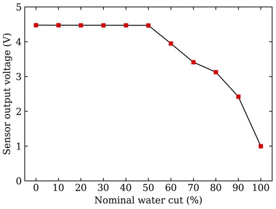
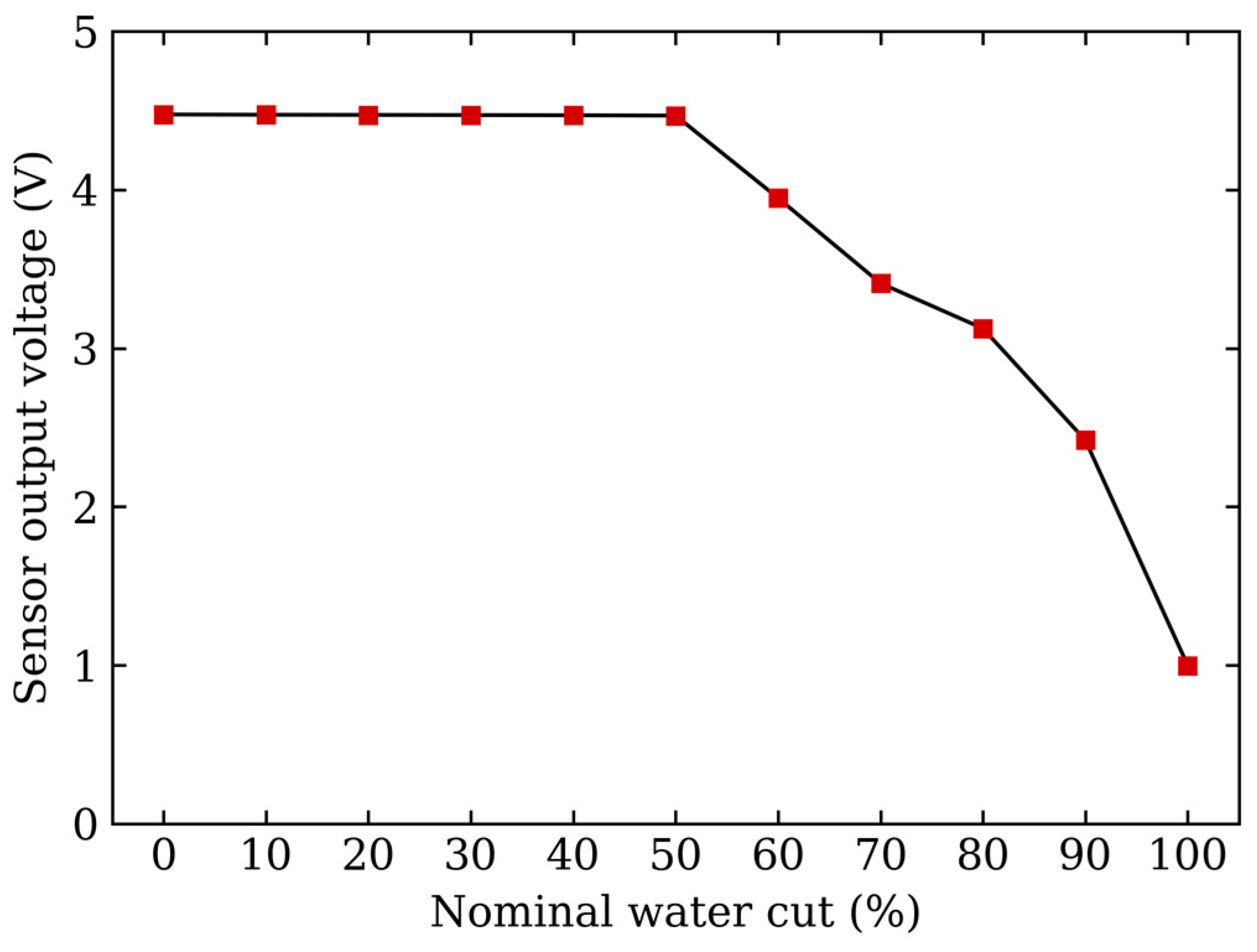
Figure 4 shows the influence of nominal water cut on the sensor output voltage at 25 °C and 0 mg/L salinity. From 0% to 40% water cut, the voltage remains close to 4.5 V, decreasing only from 4.475 to 4.470 V. The corresponding endpoint-average sensitivity is approximately −1.25 × 10⁻⁴ V per percentage point, indicating that the measured voltage is only weakly sensitive to water-cut variation in this range. This near-saturated response is consistent with limited connectivity of the conductive aqueous phase, such that changes in water cut are only weakly reflected in the macroscopic electrical response.

Figure 4. Baseline sensor output voltage versus nominal water cut at 25 °C and 0 mg/L salinity.

Above approximately 50% water cut, the output voltage decreases markedly. The endpoint-average sensitivities increase to approximately −5.20 × 10⁻² V per percentage point over 50–60% and −8.04 × 10⁻² V per percentage point over 70–100%. Although the local rate of decrease is nonuniform, the voltage response is substantially more sensitive to water cut than in the low-water-cut range. This behavior is consistent with increasing connectivity of the aqueous phase, which reduces the effective sensor impedance and consequently lowers the output voltage according to the voltage-divider relationship.

Figure 4 thus establishes the progression from weak electrical sensitivity to a much stronger voltage response above approximately 50% water cut. In the nearly flat 0–40% branch, small voltage differences can produce large inverse-prediction changes, so additional sampling density alone cannot resolve the weak measurement sensitivity. The independent accuracy evaluation therefore focuses on 55–95% nominal water cut.

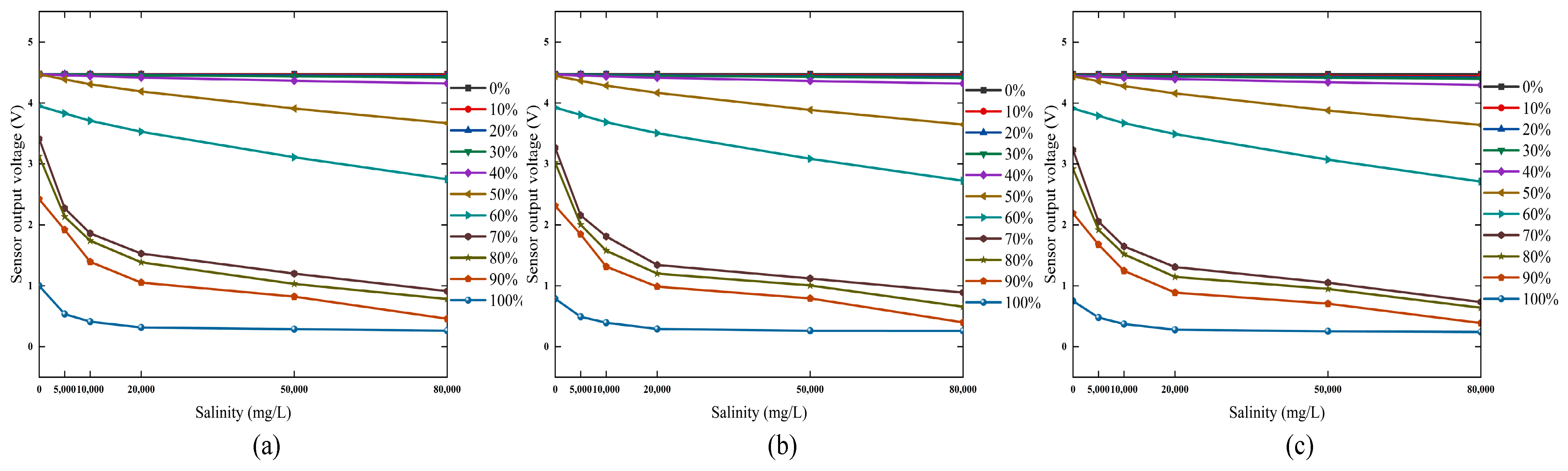
Figure 5 shows the effect of salinity on the sensor output voltage at different temperatures. In the 0–40% water-cut range, the output remains within a relatively narrow high-voltage range of approximately 4.30–4.48 V and changes only slightly with salinity. This indicates that variations in aqueous-phase conductivity are only weakly reflected in the measured voltage. Such behavior is consistent with limited connectivity of the conductive aqueous phase, where changes in ionic concentration have a relatively small influence on the bulk electrical response [11,20].

Figure 5. Sensor output voltage at different salinity levels: (a) 25 °C, (b) 45 °C, (c) 65 °C.

Above approximately 50% water cut, the dependence of voltage on salinity becomes substantially stronger. In the 50–60% range, the response exhibits pronounced nonlinear variation with salinity. This behavior is consistent with increasing connectivity of the aqueous phase, which allows changes in intrinsic aqueous conductivity to exert a greater influence on the effective sensor impedance. In the 70–100% range, the voltage decreases clearly with increasing salinity [23,24,25]. The largest overall salinity-induced variations occur around 70–80% water cut. This trend suggests that conductive pathways are more effectively developed in this range, so that increases in ionic concentration produce a stronger macroscopic electrical response.

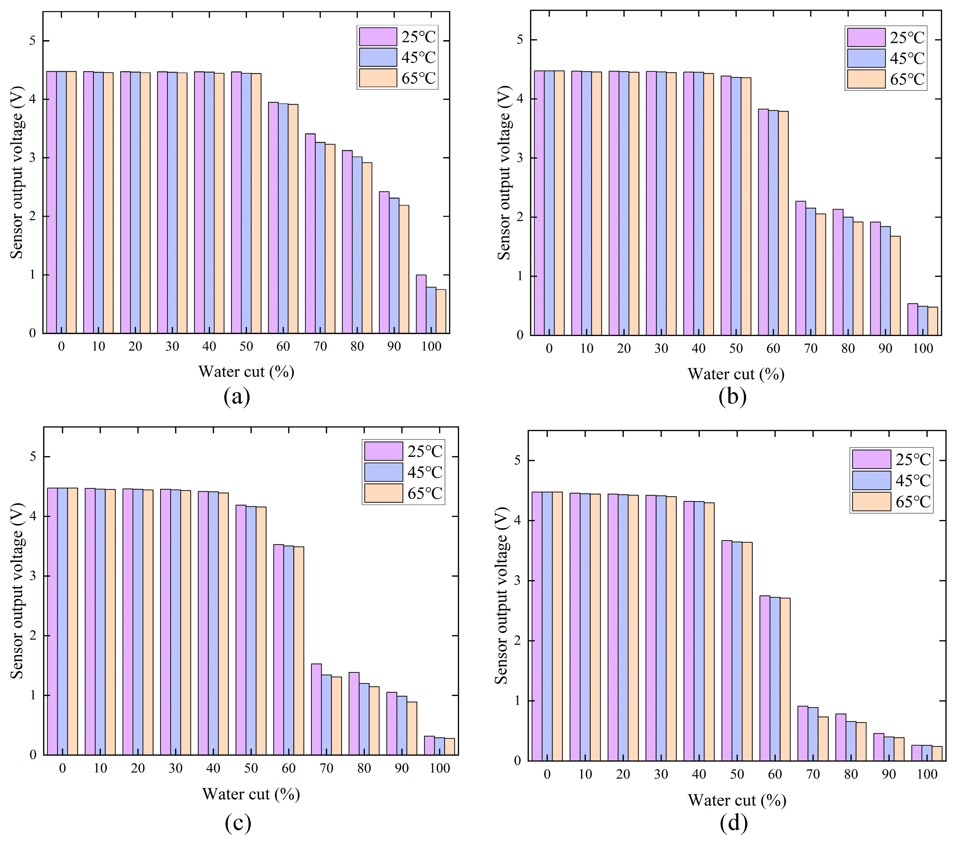
Figure 6 compares the temperature dependence at representative salinity levels of 0, 5000, 20,000, and 80,000 mg/L. At water cuts of 0–40%, the voltage curves at different temperatures remain closely grouped, indicating limited observable temperature sensitivity. Above approximately 50% water cut, the separation between the curves becomes more evident. The magnitude of the temperature effect also varies with salinity. This behavior is consistent with the combined influence of temperature-dependent ionic mobility and salinity-dependent ionic concentration on aqueous-phase conductivity. The measured response therefore reflects coupled effects of temperature, salinity, and water cut rather than the influence of any single variable.

Figure 6. Sensor output voltage at various temperatures: (a) 0 mg/L, (b) 5000 mg/L, (c) 20,000 mg/L, (d) 80,000 mg/L.

Endpoint-average sensitivity indices quantify the coupled trends. For salinity changes from 0 to 80,000 mg/L, averaged over the three temperatures, the sensitivities at 30%, 60%, and 90% water cut are approximately −0.0064, −0.150, and −0.2365 V per 10,000 mg/L. For temperature changes from 25 to 65 °C, averaged over the six salinities, the corresponding values are −0.0052, −0.0095, and −0.0403 V per 10 °C.

Together, Figure 4, Figure 5 and Figure 6 show that aqueous-path connectivity controls how strongly changes in temperature and salinity appear in the measured voltage. The stronger coupled response in the transition and high-water-cut ranges provides the experimental basis for joint compensation using V, T, and S.

4. Compensation Model Development and Performance Evaluation

The inverse model estimates nominal water cut from mean sensor peak voltage, temperature, and salinity. MPR provides an explicit ridge-regularized nonlinear basis-expansion baseline, SVR provides a nonlinear kernel-based benchmark, and BR-BPNN provides a compact multilayer estimator for embedded deployment.

The three models use common inputs and the same 9000 development samples derived from the 198 measured calibration points. Trilinear interpolation combines the eight corner voltages in each temperature–salinity–water-cut cell. The derived samples increase numerical sampling density while retaining 198 independent physical calibration observations. Internal partitions assess approximation of this response surface; the separately measured blind test and physical-plane holdouts assess prediction on physical measurements.

The derived grid comprised temperatures of 25:5:65 °C, 20 equally spaced salinities from 0 to 80,000 mg/L, and 50 equally spaced water-cut fractions from 0 to 1, giving 9000 points within the measured bounds. MATLAB (MathWorks Inc., Natick, MA, USA) griddedInterpolant applied linear interpolation along all three axes.

Common min–max normalization used t = (T − 25)/40, s = S/80,000, and v = (V − 0.241)/4.234, corresponding to T = 25–65 °C, S = 0–80,000 mg/L, and V = 0.241–4.475 V. The input order was [t,s,v]ᵀ; the target remained a fraction in [0, 1], and predictions were clamped to that interval before percentage-point errors were calculated. Automatic network preprocessing was disabled.

MPR and SVR selection used one 80/20 split of the derived data, while BR-BPNN architecture screening used five repeated splits. Each selected learned model was refitted on all 9000 derived samples and evaluated on the same 40 measured test conditions. The feature basis, partition seeds, search settings, and training record are specified in Supplementary Methods S1–S5. Additional results are provided in Tables S1–S5.

All model development is performed offline. After model comparison and independent evaluation, the finalized BR-BPNN is deployed on the STM32L496RGT3 microcontroller. Only forward inference is performed during embedded operation. This offline-training and online-inference strategy limits the computational burden during real-time measurement.

4.1. Ridge-Regularized Nonlinear Basis Expansion (MPR)

MPR provides an explicit ridge-regularized nonlinear basis-expansion baseline (referred to as MPR for brevity) for the inverse mapping Y_w = G(V,T,S). Data-generation methods have also been investigated for nonlinear temperature compensation in piezoresistive sensors [26]. Here, the common normalized inputs are expanded into a 27-term nonlinear feature vector:

X_n = ϕ(t_n,s_n,v_n)

(7)

where ϕ(·) denotes the feature-mapping operator and X_n is the expanded vector for sample n. The inputs t_n, s_n, and v_n are normalized temperature, salinity, and voltage. The basis combines polynomial and interaction terms, higher-order voltage terms, and selected reciprocal, exponential, and square-root terms; its ordered definition and coefficient-selection settings are provided in Supplementary Methods S2.

The expanded basis contains correlated terms, so ridge regularization is used to stabilize coefficient estimation [27]. The regression coefficients are obtained from

$$\widehat{\beta }=\arg {\min }_{\beta }\left\{{‖Y_{\mathrm{w}}-\mathit{X\beta }‖}_2^2+\lambda {‖\beta ‖}_2^2\right\}$$

(8)

where X is the input feature matrix, β is the regression coefficient vector, $\widehat{\beta }$ is the optimized coefficient vector, and λ is the ridge regularization parameter. The ridge penalty was selected by validation RMSE on an 80/20 split generated with rng(8100), evaluating 30 logarithmically spaced values from 10⁻⁸ to 10¹. The final coefficients were refitted on all 9000 samples with λ = 10⁻⁸.

The explicit feature basis provides an interpretable approximation of the global response. Its performance in the nonlinear transition and high-salinity regions is assessed against SVR and BR-BPNN in Section 4.4.

4.2. Support Vector Regression

SVR uses the same normalized input vector x = [t,s,v]ᵀ. A Gaussian radial-basis-function kernel represents nonlinear dependence through similarity in the input space:

$$K(x_i,x_j)=\exp \left[-{\displaystyle \frac{{‖x_i-x_j‖}_2^2}{2{\mathsf{\ell }}^2}}\right]$$

(9)

where x_i and x_j denote the normalized input vectors of samples i and j, respectively; ‖⋅‖₂ denotes the Euclidean norm; and ℓ > 0 is the Gaussian kernel scale. Smaller values of ℓ yield a more localized kernel response, whereas larger values produce a smoother response over the input space.

The corresponding ε-SVR predictor is written as:

$${\widehat{Y}}_{\mathrm{w}}(x)={\displaystyle {\displaystyle \sum _{i=1}^N}({\alpha }_i-{\alpha }_i^{*})K(x_i,x)}+b$$

(10)

where α_i and α_i^* are the optimized support vector coefficients and b is the bias term.

The parameters C, ε, and ℓ control the deviation penalty, insensitive width, and Gaussian kernel scale. Validation RMSE on an 80/20 split generated with rng(9100) was used to search C ∈ {1, 10, 100}, ε ∈ {0.005, 0.01, 0.02, 0.05}, and ℓ ∈ {0.1, 0.3, 1}. The selected values were C = 100, ε = 0.01, and ℓ = 0.1. The model was refitted on all 9000 samples with Standardize = false because the common normalization had already been applied.

Recent measurement studies further support the use of SVR for nonlinear sensor modeling and error compensation. Liu et al. [28] applied a DOA-optimized SVR to correct a surface-acoustic-wave yarn-tension transducer and reported better test-set performance than multiple regression and BP neural network models. Dang et al. [29] used SVR to model the nonlinear input–output behavior of an ultrasonic sensor. More directly in multiphase flow metering, Pereira et al. [30] applied SVR to estimate gas and liquid flow rates under wet-gas conditions and found that the nonlinear SVR consistently outperformed a linear partial-least-squares model. These studies support the use of SVR as an appropriate nonlinear kernel benchmark in the present work.

Compared with the fixed basis expansion used by MPR, the SVR kernel can represent localized nonlinear variation through support vector similarities. It provides a complementary nonlinear benchmark for the multilayer BR-BPNN.

4.3. Bayesian Regularized Backpropagation Neural Network

The experimental results show strong nonlinear coupling in the response-transition range and under high-salinity conditions. BR-BPNN is introduced to better capture these coupled nonlinear effects. Unlike explicit regression, the network learns the input–output mapping through nonlinear transformations in hidden layers. Neural network methods have been widely applied to phase-fraction estimation, flow-pattern identification, and related multiphase-flow inverse problems [31,32].

Four topologies—3-5-1, 3-10-1, 3-8-4-1, and 3-10-5-1—were screened using five random 80/20 partitions of the derived data with seeds 5001–5005. Initialization used rng(10000 + 100*r + a), where r indexes the partition and a indexes the architectures in the stated order. Selection considered validation RMSE, MAE, and computational complexity. The chosen 3-10-5-1 network takes normalized [t,s,v]ᵀ as input, uses 10 and 5 neurons in the hidden layers, and outputs Y_w. It contains 101 trainable parameters and requires 85 weight multiplications per forward inference, excluding activation-function evaluation.

During forward propagation, each layer applies an affine transformation followed by the specified activation function. The hidden- and output-layer responses are expressed as

$$O_i^{(1)}=f_1\left({\displaystyle \sum _{j=1}^3{w}_{\mathit{ij}}^{(1)}}{X}_j+b_i^{(1)}\right)$$

(11)

$$O_k^{(2)}=f_1\left({\displaystyle \sum _{i=1}^{10}{w}_{\mathit{ki}}^{(2)}}{O}_i^{(1)}+b_k^{(2)}\right)$$

(12)

$$Y_{\mathrm{w}}=f_2\left({\displaystyle \sum _{k=1}^5{w}_{\mathit{lk}}^{(3)}}{O}_k^{(2)}+b_l^{(3)}\right)$$

(13)

where X_j is the j-th input variable, and O_i⁽¹⁾ and O_k⁽²⁾ are the outputs of the first and second hidden layers. The parameters w and b denote connection weights and biases. Both hidden layers use the hyperbolic tangent activation function f₁, while the output layer uses the linear activation function f₂. The corresponding bias terms are b_i⁽¹⁾, b_k⁽²⁾, and b_l⁽³⁾.

A conventional BP network trained only to minimize data error can overfit a limited calibration set. Bayesian regularization addresses this problem by penalizing excessive parameter magnitude. The resulting objective balances data fitting and model complexity [33,34,35]:

F(w) = β_BRE_D + α_BRE_W

(14)

where F(w) is the Bayesian regularization objective, w contains all network weights and biases, E_D is the sum of squared prediction errors, and E_W is the sum of squared network parameters. The coefficients α_BR and β_BR are adaptive regularization parameters.

$$\left\{\begin{array}{l}{E}_{\mathrm{W}}={\displaystyle \sum _{m=1}^n{w}_m^2}\hfill \\ E_{\mathrm{D}}={\displaystyle \sum _{k=1}^N{\left(Y_{\mathrm{w},k}-{\widehat{Y}}_{\mathrm{w},k}\right)}^2}\hfill \end{array}\right.$$

(15)

where N is the number of training samples, and Y_w,k and ${\widehat{Y}}_{\mathrm{w},k}$ are the reference and predicted water-cut values for sample k, respectively. The symbol w_m denotes the m-th trainable parameter, and n is the total number of network parameters.

Bayesian regularization updates α_BR and β_BR during training to balance data fidelity and parameter regularization [33,34,35]. This adaptive weighting reduces the need for manual selection of a fixed regularization coefficient. In the present implementation, the effective number of parameters converged to γ_eff = 91.23 out of 101 trainable parameters.

The recorded parameter sum of squares was ssX = 1.295 × 10⁴. The final network was trained on all 9000 samples in MATLAB R2024b (MathWorks Inc., Natick, MA, USA) Update 2 with Deep Learning Toolbox 24.2, using fitnet([10 5],’trainbr’), divideFcn = ‘dividetrain’, tansig hidden layers, and a purelin output. Initialization used rng(42); training reached the preset 1000-epoch limit. The architecture-screening and training record is provided in Supplementary Methods S4; normalization is specified in Supplementary Methods S1.

Reliability of Interpolation-Based Training

A retrospective training-strategy comparison used the same topology with (A) 198 measured samples, (B) 9000 repetitions of measured samples, and (C) 9000 trilinearly derived samples. Across three initializations, mean test MAE was 5.077, 8.120, and 1.566 pp, respectively, with lower initialization variability for interpolation (Table S1). The improvement reflects sampling of the fitted response surface rather than an increase in independent physical information; interpolation bias can propagate into the learned inverse.

Forward interpolation on the 40 measured test conditions gave voltage MAE = 0.068757 V, RMSE = 0.081119 V, R² = 0.99481, and maximum absolute residual = 0.17805 V. Eight physical-plane holdouts rebuilt the response surface after removing the evaluated plane, with two initializations per strategy (Table S3). Interpolation gave the lowest mean MAE on seven planes, but the 70% water-cut plane yielded 7.878 pp versus 4.891 pp for measured-only training. On the 45 °C plane, mean MAE was 2.522 pp and the mean maximum absolute error was 29.147 pp. Such outliers are consistent with the weak low-water-cut sensitivity in Figure 4, where inversion amplifies small voltage differences.

4.4. Model Comparison and Performance Evaluation

The blind-test matrix contains 40 measured combinations: 35 and 55 °C; NaCl salinities of 3500, 6500, 25,000, and 65,000 mg/L; and nominal water cuts of 55%, 65%, 75%, 85%, and 95%. Fresh preparation and direct voltage acquisition followed Section 3.1. Original model selection was completed before inspection of these test errors; subsequent training-strategy and direct-inversion comparisons reuse the same measurements as retrospective analyses.

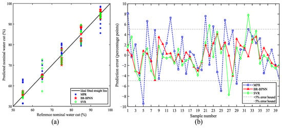
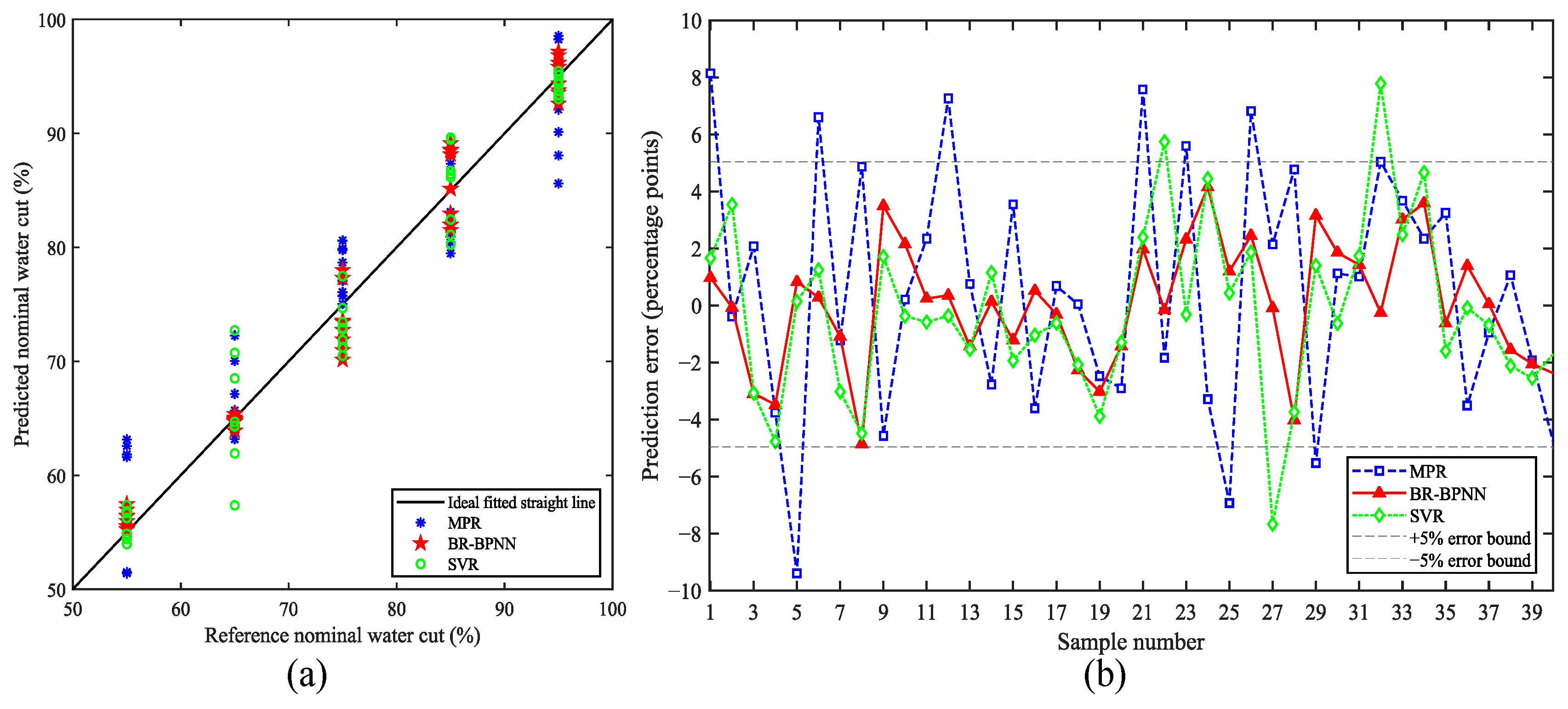
Figure 7a shows the performance of the fitted candidates on the shared 40-condition test set. BR-BPNN predictions lie closest to the ideal 1:1 line overall. SVR follows the reference trend, with larger deviations at several operating points, while MPR shows the widest dispersion, particularly around reference water cuts of 55%, 65%, and 95%.

Figure 7. Offline validation on the 40 measured test conditions: (a) predicted versus reference nominal water cut, with the solid line indicating ideal 1:1 agreement; (b) sample-wise prediction errors, with dashed lines indicating ±5 percentage-point bounds.

Figure 7b shows that all offline BR-BPNN errors remain within ±5 pp, with a maximum absolute error of 4.8488 pp. MPR exhibits the largest fluctuations and several excursions beyond ±5 pp, reaching 9.3940 pp. SVR improves on MPR overall but still has deviations exceeding 7 pp, with a maximum absolute error of 7.7235 pp. The sample-wise distributions complement the aggregate metrics in Table 1.

Table 1. Performance of the evaluated methods on the same 40 measured test conditions. Water-cut errors are in percentage points (pp).

Model	R2	RMSE (pp)	MAE (pp)	AEmax (pp)
BR-BPNN	0.97656	2.1652	1.7233	4.8488
Direct trilinear inversion	0.97026	2.4388	1.7974	5.5991
SVR	0.95535	2.9884	2.3175	7.7235
MPR	0.90946	4.2553	3.5215	9.3940

Four metrics are used for quantitative evaluation: the coefficient of determination (R²), root mean square error (RMSE), mean absolute error (MAE), and maximum absolute error (AEmax):

$$R^2=1-{\displaystyle \frac{{\displaystyle \sum _{i=1}^n{(y_i-{\widehat{y}}_i)}^2}}{{\displaystyle \sum _{i=1}^n{(y_i-\overline{y})}^2}}}$$

(16)

$$\mathit{RMSE}=\sqrt{{\displaystyle \frac{1}{n}}{\displaystyle \sum _{i=1}^n{(y_i-{\widehat{y}}_i)}^2}}$$

(17)

$$\mathit{MAE}={\displaystyle \frac{1}{n}}{\displaystyle \sum _{i=1}^n|}{y}_i-{\widehat{y}}_i|$$

(18)

$$\mathit{AEmax}={\max }_{1\le i\le n}|y_i-{\widehat{y}}_i|$$

(19)

where y_i is the reference value, ${\widehat{y}}_i$ is the predicted value, $\overline{y}$ is the mean reference value, and n is the number of samples.

On the same 40 measured conditions, BR-BPNN achieved R² = 0.97656, RMSE = 2.1652 pp, and MAE = 1.7233 pp, compared with RMSE/MAE = 2.9884/2.3175 pp for SVR and 4.2553/3.5215 pp for MPR. Direct trilinear inversion achieved RMSE = 2.4388 pp and MAE = 1.7974 pp. This ranking describes the specific fitted candidates under the reported preprocessing and model-selection procedures. The common test set supports comparison under identical measured conditions, but the different selection splits and search procedures do not isolate an intrinsic advantage of one model class or establish statistical superiority.

Direct trilinear inversion uses the same 198-point forward calibration grid without fitted regression coefficients. At each measured T and S, bilinear interpolation gives nodal voltages for water-cut fractions 0.50, 0.60, …, 1.00. Non-flat segments yield piecewise-linear inverse candidates. Multiple candidates are resolved by the smallest forward-voltage residual; when no segment is admissible, the nearest-voltage branch node is returned. Supplementary Methods S5 specifies the numerical tolerances, tie rule, and final bounds. BR-BPNN instead encodes the inverse mapping in 101 fixed parameters and 85 weight multiplications plus activations, avoiding runtime grid lookup and inverse interpolation. Execution time for direct inversion was not measured on the STM32, so the deployment comparison is limited to this structural distinction.

4.4.1. Condition-Wise Prediction Error

Signed error is predicted minus reference nominal water cut. There are 20 test samples per temperature, 10 per salinity, and 8 per water-cut level. BR-BPNN MAE was 1.561 pp at 35 °C and 1.885 pp at 55 °C, with mean signed errors of −0.659 and +0.777 pp. Salinity subgroup MAE ranged from 1.230 pp at 25,000 mg/L to 2.345 pp at 6500 mg/L. MAE was higher at 75–85% water cut (2.815–2.885 pp) than at 65% (0.294 pp); the salinity subgroup errors showed no monotonic trend in this test matrix. Table S4 provides the full descriptive breakdown.

4.4.2. Sensitivity to Externally Supplied Salinity

Relative salinity offsets were imposed numerically on the 40 measured voltage–temperature pairs while holding V, T, and the trained weights fixed. Positive offsets of +5% and +10% increased MAE from 1.7233 pp to 1.8579 and 2.0116 pp, RMSE to 2.4111 and 2.8203 pp, and maximum absolute error to 5.5118 and 6.8393 pp. Negative offsets reduced aggregate MAE on this test set, indicating an asymmetric response. Averaging the mean absolute prediction shifts for equal positive and negative perturbations gave 0.1093, 0.5453, and 1.0824 pp at magnitudes of 1%, 5%, and 10%, respectively (Table S2).

4.4.3. Comparison with Related Studies

Table 2 positions the present work alongside conductance-based holdup studies [10,11] and established data-driven compensation and water-content methods [12,14]. Each entry retains its original sensing modality, target definition, operating range, and error metric. The present contribution combines measured conductance-response characterization, evaluated interpolation-based training, and compact embedded compensation.

Table 2. Related measurement and compensation studies. Target quantities and error definitions are reported as in the original publications.

Study	Sensing Method and Target	Study-Specific Conditions	Performance as Reported
Wang et al. [10]	Conductance/water holdup	Water cut 30–90%; flow 10–200 m3/d	Absolute holdup error < 5%
Han et al. [11]	Phase-state regulation + conductance/holdup	High-holdup, low-rate oil-water flow	Holdup accuracy better than 3.23%
Dai et al. [12]	BO-XGBoost, multi-sensor/water holdup	0–100% water holdup	Average absolute error 1.50%
Zhang and Xia [14]	Dielectric multi-sensor; RS-SVM + GA-NN/water content	Water content 0–100%; T 20–90 °C; salinity 0–50 g/L	MAE 0.76%; AEmax 2.3%
Present study	Conductance + BR-BPNN/nominal prepared water cut	Independent tests: 55–95%; 35/55 °C; fixed 30 m3/d	Offline MAE 1.7233 pp; STM32 MAE 1.8680 pp

4.5. STM32 Embedded Implementation and Experimental Verification

After offline training and independent algorithm evaluation, the finalized 3-10-5-1 BR-BPNN was deployed on the STM32L496RGT3 microcontroller. The trained weights, biases, and preprocessing parameters were embedded directly into the firmware. No online weight updating, backpropagation, or parameter optimization was performed during operation.

Embedded verification repeated the same 40 nominal temperature–salinity–water-cut conditions with newly acquired sensor voltages. Each voltage was combined with the corresponding temperature and externally supplied salinity, while the network architecture and trained parameters remained fixed. This evaluated the acquisition-and-inference implementation under repeated laboratory measurements.

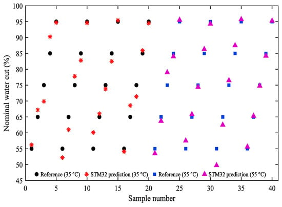
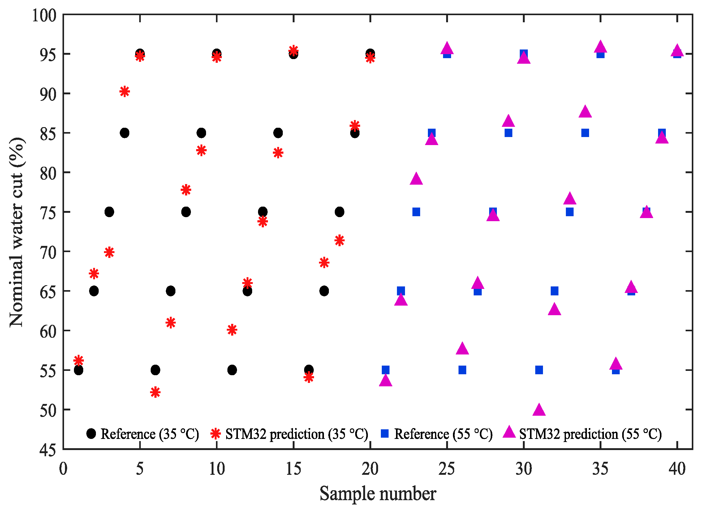
The STM32 evaluation achieved R² = 0.97079, RMSE = 2.4170 pp, MAE = 1.8680 pp, and maximum absolute error = 5.2400 pp. Relative to the offline evaluation, MAE increased by 0.1447 pp (about 8.4%) and RMSE by 0.2518 pp. Figure 8 compares the 40 STM32 predictions with the nominal references; individual values are listed in Table S5. Possible contributors include acquisition noise, temperature and phase-distribution variation between repeated loop measurements, and firmware numerical precision. These contributions were not separately isolated, so the observed difference is interpreted as the overall deployment-and-remeasurement result.

Figure 8. STM32-based BR-BPNN predictions and reference nominal water cuts for 40 test conditions. Samples 1–20 correspond to 35 °C and 21–40 to 55 °C. Within each temperature group, successive five-sample blocks correspond to salinities of 3500, 6500, 25,000, and 65,000 mg/L; reference water cuts increase from 55% to 95% within each block.

Network execution time was measured separately on the 72 MHz STM32L496RGT3 using the Cortex-M4 DWT cycle counter. Five representative temperature–salinity combinations were tested at a fixed 2.5 V timing input. After 10 warm-up inferences, 1000 runs were timed per condition. Across 5000 measurements, mean forward-inference time was 52.05 μs, condition means ranged from 50.20 to 53.26 μs, and the maximum was 55.49 μs. This interval covers network computation and excludes sensor sampling, FPGA processing and communication, temperature acquisition, and CAN transmission; full sensor-to-result latency was not measured.

According to the ARMCC linker report, the complete firmware occupies 15,104 bytes of Flash and 2008 bytes of RAM. These values include peripheral drivers, acquisition and communication routines, temperature processing, and BR-BPNN inference, and therefore represent the complete firmware rather than the neural network alone. The deployed 3-10-5-1 network contains 101 trainable parameters and requires 85 weight multiplications per forward inference, excluding activation-function operations. The measured latency and memory footprint confirm that the model can operate within the computational resources of the target microcontroller.

5. Conclusions

This study investigated the coupled effects of temperature, salinity, and water cut on conductance-based water-cut measurement. The calibration experiments showed that the sensor voltage is only weakly sensitive to water-cut variation in the low-water-cut range. In contrast, the response becomes substantially more sensitive to water cut, temperature, and salinity above approximately 50% water cut. These observations show that multi-parameter compensation is particularly important in the response-transition and high-water-cut ranges.

Using 198 measured calibration points and 9000 trilinearly derived samples, the study evaluated fitted MPR, SVR, and BR-BPNN candidates under their reported selection procedures on 40 separately measured conditions spanning 55–95% nominal water cut. In this comparison, BR-BPNN achieved the lowest MAE and RMSE among these three candidates, with R² = 0.97656, RMSE = 2.1652 percentage points, MAE = 1.7233 percentage points, and maximum absolute error = 4.8488 percentage points. Training-strategy and physical-plane analyses further characterized the accuracy and local variability of interpolation-based training.

The fixed 3-10-5-1 network was deployed on the STM32L496RGT3 and evaluated with newly acquired sensor signals, achieving R² = 0.97079, RMSE = 2.4170 percentage points, MAE = 1.8680 percentage points, and maximum absolute error = 5.2400 percentage points. The implementation retained similar overall accuracy to the offline model.

The average BR-BPNN forward-inference latency was 52.05 μs at a system clock frequency of 72 MHz, with a maximum measured latency of 55.49 μs. The complete firmware occupied 15,104 bytes of Flash and 2008 bytes of RAM. Together with the measured prediction errors, these results demonstrate that the selected compact network operates within the computational resources of the target STM32 platform.

Independent validation covers 55–95% nominal water cut at two temperatures and four NaCl salinities under fixed flow and stirring conditions. Future work will extend physical validation to lower water cuts, different flow regimes, produced-water compositions, and repeated measurements, and evaluate salinity-update timing and end-to-end latency. Identical-input offline-embedded comparisons and a common model-selection protocol will further distinguish numerical effects and model-dependent performance.

References

- Dai, R.; Jin, N.; Hao, Q.; Ren, W.; Zhai, L. Measurement of Water Holdup in Vertical Upward Oil–Water Two-Phase Flow Pipes Using a Helical Capacitance Sensor. Sensors 2022, 22, 690. [Google Scholar] [CrossRef] [Scilit]
- Abbagoni, B.M.; Yeung, H.; Lao, L. Non-invasive measurement of oil-water two-phase flow in vertical pipe using ultrasonic Doppler sensor and gamma ray densitometer. Chem. Eng. Sci. 2022, 248, 117218. [Google Scholar] [CrossRef] [Scilit]
- Liu, W.; Jin, N.; Wang, D.; Han, Y.; Ma, J. A parallel-wire microwave resonant sensor for measurement of water holdup in high water-cut oil-in-water flows. Flow Meas. Instrum. 2020, 74, 101760. [Google Scholar] [CrossRef] [Scilit]
- Jin, N.; Zhou, Y.; Liang, X.; Wang, D.; Zhai, L.; Wei, J. Flow Measurement of Oil-Water Two-Phase Flow at Low Flow Rate Using the Plug-in Conductance Sensor Array. Sensors 2019, 19, 4649. [Google Scholar] [CrossRef] [Scilit]
- Ma, J.; Jin, N.; Wang, D.; Liu, D.-Y.; Liu, W.-X. Measurement of water holdup in vertical upward high water-cut oil-in-water flows using a high frequency sensor. Sens. Actuators A Phys. 2019, 289, 165–179. [Google Scholar] [CrossRef] [Scilit]
- Zhou, Y.; Jin, N.; Zhang, H.; Zhai, L. Method based on parallel-wire conductivity probe for measuring water hold-up in near-horizontal oil–water two-phase flow pipes. IET Sci. Meas. Technol. 2020, 14, 676–683. [Google Scholar] [CrossRef] [Scilit]
- Zuo, K.; Hong, Y.; Qi, H.; Li, Y.; Li, B. Application of Microwave Transmission Sensors for Water Cut Metering under Varying Salinity Conditions: Device, Algorithm and Uncertainty Analysis. Sensors 2022, 22, 9746. [Google Scholar] [CrossRef] [Scilit]
- Shi, X.; Tan, C.; Dong, F.; dos Santos, E.N.; da Silva, M.J. Conductance Sensors for Multiphase Flow Measurement: A Review. IEEE Sens. J. 2021, 21, 12913–12925. [Google Scholar] [CrossRef] [Scilit]
- Wiedemann, P.; Dias, F.D.A.; Schleicher, E.; Hampel, U. Temperature Compensation for Conductivity-Based Phase Fraction Measurements with Wire-Mesh Sensors in Gas-Liquid Flows of Dilute Aqueous Solutions. Sensors 2020, 20, 7114. [Google Scholar] [CrossRef] [Scilit]
- Wang, Y.; Han, J.; Hao, Z.; Zhou, L.; Wang, X.; Shao, M. A New Method for Measuring Water Holdup of Oil-Water Two-Phase Flow in Horizontal Wells. Processes 2022, 10, 848. [Google Scholar] [CrossRef] [Scilit]
- Han, L.; Chen, M.; Liu, X.; Fu, C. New Measurement Method of Oil-Water Two-Phase Flow with High Water Holdup and Low Rate by Phase State Regulation. Meas. Sci. Rev. 2023, 23, 268–274. [Google Scholar] [CrossRef] [Scilit]
- Dai, X.; Wei, Y.; Gan, R.; Wei, B.; Xiang, Y.; Liu, P. Research on Correction of Temperature and Mineralization and Prediction of Water Holdup Based on Machine Learning. IEEE Access 2024, 12, 100377–100388. [Google Scholar] [CrossRef] [Scilit]
- Yan, Y.; Wang, L.; Wang, T.; Wang, X.; Hu, Y.; Duan, Q. Application of soft computing techniques to multiphase flow measurement: A review. Flow Meas. Instrum. 2018, 60, 30–43. [Google Scholar] [CrossRef] [Scilit]
- Zhang, D.; Xia, B. Soft Measurement of Water Content in Oil-Water Two-Phase Flow Based on RS-SVM Classifier and GA-NN Predictor. Meas. Sci. Rev. 2014, 14, 219–226. [Google Scholar] [CrossRef] [Scilit]
- Khrapak, S.; Khrapak, A. Stokes–Einstein Relation in Different Models of Water. Molecules 2024, 29, 5587. [Google Scholar] [CrossRef] [Scilit]
- Mizuhata, M. Electrical Conductivity Measurement of Electrolyte Solution. Electrochemistry 2022, 90, 102011. [Google Scholar] [CrossRef] [Scilit]
- Zhang, W.; Chen, X.; Wang, Y.; Wu, L.; Hu, Y. Experimental and Modeling of Conductivity for Electrolyte Solution Systems. ACS Omega 2020, 5, 22465–22474. [Google Scholar] [CrossRef] [Scilit]
- Dorn, M.; Kareth, S.; Weidner, E.; Petermann, M. Electrical Conductivity of Lithium, Sodium, Potassium, and Quaternary Ammonium Salts in Water, Acetonitrile, Methanol, and Ethanol over a Wide Concentration Range. J. Chem. Eng. Data 2024, 69, 1493–1502. [Google Scholar] [CrossRef] [Scilit]
- Bai, L.; Jin, N.; Zhang, J.; Ouyang, L.; Wang, C. Experimental study of oil-water two-phase flow patterns in a vertical large diameter pipe. Flow Meas. Instrum. 2024, 99, 102681. [Google Scholar] [CrossRef] [Scilit]
- Tan, J.; Luo, P.; Vahaji, S.; Jing, J.; Hu, H.; Yu, B.; Tu, J. Experimental investigation on phase inversion point and flow characteristics of heavy crude oil-water flow. Appl. Therm. Eng. 2020, 180, 115777. [Google Scholar] [CrossRef] [Scilit]
- Song, Z.; Han, G.; Ren, Z.; Su, H.; Jia, S.; Cheng, T.; Li, M.; Liang, J. Research on Oil–Water Two-Phase Flow Patterns in Wellbore of Heavy Oil Wells with Medium-High Water Cut. Processes 2024, 12, 2404. [Google Scholar] [CrossRef] [Scilit]
- Texas Instruments. ADS866x 12-Bit, High-Speed, Single-Supply SAR ADC Data Acquisition System with Programmable Bipolar Input Ranges; Datasheet SBAS780B, Rev. B.; Texas Instruments: Dallas, TX, USA, 2021; Available online: https://www.ti.com/lit/ds/symlink/ads8665.pdf (accessed on 29 October 2026).
- Sun, X.; Wang, N.; Hou, L.; Liu, X.; Gu, A. Flow characteristics of high-water-content heavy oil-water mixtures in pipeline transport: Experimental investigation and engineering implications. Energy 2026, 345, 140193. [Google Scholar] [CrossRef] [Scilit]
- Yang, Y.; Ha, W.; Zhang, C.; Liu, M.; Zhang, X.; Wang, D. Measurement of high-water-content oil-water two-phase flow by electromagnetic flowmeter and differential pressure based on phase-isolation. Flow Meas. Instrum. 2022, 84, 102142. [Google Scholar] [CrossRef] [Scilit]
- Lyu, Y.; Huang, Q. Flow characteristics of heavy oil-water flow during high water-content cold transportation. Energy 2023, 262, 125441. [Google Scholar] [CrossRef] [Scilit]
- Zou, M.; Xu, Y.; Jin, J.; Chu, M.; Huang, W. Accurate Nonlinearity and Temperature Compensation Method for Piezoresistive Pressure Sensors Based on Data Generation. Sensors 2023, 23, 6167. [Google Scholar] [CrossRef] [Scilit]
- Guzman-Chavez, A.D.; Vargas-Rodriguez, E. The Application of Kernel Ridge Regression for the Improvement of a Sensing Interferometric System. Sensors 2025, 25, 1292. [Google Scholar] [CrossRef] [Scilit]
- Liu, S.; Wang, D.; Xing, R.; Ren, J.; Lu, W. Research on error correction model of surface acoustic wave yarn tension transducer based on DOA–SVR model. Measurement 2024, 226, 114126. [Google Scholar] [CrossRef] [Scilit]
- Dang, D.N.; Do, T.M.; de Matos Araújo, R.A.; Nguyen, K.H.V.; Le, C.D. Ultrasonic sensor modeling with support vector regression. Sensors 2025, 25, 678. [Google Scholar] [CrossRef] [Scilit]
- Pereira, L.O.V.; Farias, M.H.; Rocha, W.F.C.; Franco, L.G.; Ramos, R. Machine learning-based prediction of gas and liquid flow rates in wet gas using single and dual cone meter configurations. Flow Meas. Instrum. 2026, 111, 103453. [Google Scholar] [CrossRef] [Scilit]
- He, H.; Zhou, Z.; Sun, B.; Li, X.; Sun, X. Study on the prediction method of oil-water two-phase flow pattern and oil holdup. Geoenergy Sci. Eng. 2025, 246, 213627. [Google Scholar] [CrossRef] [Scilit]
- Bahrami, S.; Alamdari, S.; Farajmashaei, M.; Behbahani, M.; Jamshidi, S.; Bahrami, B. Application of artificial neural network to multiphase flow metering: A review. Flow Meas. Instrum. 2024, 97, 102601. [Google Scholar] [CrossRef] [Scilit]
- Truong, T.T.; Airao, J.; Hojati, F.; Ilvig, C.F.; Azarhoushang, B.; Karras, P.; Aghababaei, R. Data-driven prediction of tool wear using Bayesian regularized artificial neural networks. Measurement 2024, 238, 115303. [Google Scholar] [CrossRef] [Scilit]
- Aucejo, M.; De Smet, O. An optimal Bayesian regularization for force reconstruction problems. Mech. Syst. Signal Process. 2019, 126, 98–115. [Google Scholar] [CrossRef] [Scilit]
- Chen, H.; Sun, Z.; Zhong, Z.; Huang, Y. Fatigue Factor Assessment and Life Prediction of Concrete Based on Bayesian Regularized BP Neural Network. Materials 2022, 15, 4491. [Google Scholar] [CrossRef] [Scilit]
Disclaimer/Publisher’s Note: The statements, opinions and data contained in all publications are solely those of the individual author(s) and contributor(s) and not of MDPI and/or the editor(s). MDPI and/or the editor(s) disclaim responsibility for any injury to people or property resulting from any ideas, methods, instructions or products referred to in the content. |
© 2026 by the authors. Licensee MDPI, Basel, Switzerland. This article is an open access article distributed under the terms and conditions of the Creative Commons Attribution (CC BY) license.