


Abstract
In today’s world of rapidly evolving internet communication, email remains a widely used medium for direct message exchange across ordinary users, organizations, and defense-related environments, where spam campaigns can threaten operational continuity and communication integrity. Despite significant advances in spam filtering techniques using deep learning approaches, comparatively less attention has been given to the robustness of traditional machine learning classifiers under cross-corpus distribution shift. This study benchmarks five classical classifiers—Naive Bayes, Logistic Regression, Random Forest, Linear Support Vector Machine (SVM), and XGBoost—for spam email detection. A unified framework incorporating text preprocessing, TF-IDF feature extraction, engineered metadata features, stratified 10-fold cross-validation, and cross-corpus evaluation was applied to the sampled public email corpora, including one LLM-generated synthetic corpus (Dataset C). Classifier performance was assessed using standard classification metrics, dependence-aware statistical testing, retention-based analysis, and confusion-matrix evaluation. Corpus characteristics were examined using lexical diversity, vocabulary overlap, TF-IDF sparsity, and metadata distribution analyses. Results showed that Linear SVM achieved the highest within-corpus F1-score in the sampled conventional corpora (0.9868 on Dataset A), but this ranking did not consistently carry over to the tested transfers, where performance varied by classifier, feature set, and direction. XGBoost with combined features achieved an F1-score of 0.9233 in the A-to-C transfer, while Linear SVM achieved 0.9437 in B-to-C; these results do not establish general model rankings. Metadata-only scores above the within-corpus baseline in some transfers were consistent with the target class composition, including all-spam predictions, and do not establish a transferable metadata effect. The findings are limited to the sampled corpora and experimental settings; transfer to Dataset C does not establish generalization to LLM-generated spam more broadly.
1. Introduction
With the continuous development of internet communication technologies, email remains a widely used, versatile means of communication among individuals and organizations. Email enables simple, direct message transmission and has become an essential part of global communication, facilitating exchanges across social, professional, and institutional settings [1].
Email’s widespread adoption and continued relevance have also made it a persistent target for cybercriminals. Although unsolicited email has been recognized as a problem for decades, spam has evolved alongside technological advances, adopting increasingly sophisticated forms that challenge traditional security measures. Modern phishing emails are increasingly polished, personalized, and convincing. A recent study estimates that unsolicited messages, commonly known as spam, account for approximately 3.4 billion messages sent daily, while email serves more than 4 billion users worldwide [2]. These figures illustrate the scale of potential exposure associated with modern email communication. Historical incidents, such as the 2007 Nordea banking breach, further demonstrate the long-standing impact of phishing-based email attacks [3].
Early approaches to combating spam mainly relied on traditional filtering methods, including predefined rules and policy-based strategies to mitigate risk. These systems employed extensive blocklists and allowlists, checksums, and heuristic tests to identify spam patterns through characteristics such as excessive punctuation, capital letters, suspicious URLs, and attachments containing malware [4,5].
Although traditional spam filtering methods remain widely deployed, cybercriminals have since refined their social engineering strategies, enabling spam to appear more persuasive and legitimate, thereby creating challenges for digital environments with low risk tolerance. Sophisticated language structures, improved grammatical correctness, and contextually relevant content render traditional filtering methods inadequate. Recent advances in text-generation technologies have further increased the difficulty of distinguishing spam from legitimate email and detecting it reliably.
With the rise in artificial intelligence, machine learning algorithms continue to support a wide range of applications, including spam classification. These models learn patterns from training data and apply them to new information; in this case, they predict email classes. Various researchers have conducted experimental work on classical ML algorithms under different evaluation conditions. Bountakas et al. [6] compare combinations of different natural language processing (NLP) techniques and classical ML algorithms. Their results provide insights into how feature-extraction techniques and dataset composition affect model performance.
Owing to their ability to capture complex lexical, syntactic, and semantic patterns, deep learning (DL) models have also been widely adopted in modern spam-filtering frameworks. Numerous studies have reported improvements in classification performance, highlighting the effectiveness of architectures such as convolutional neural networks (CNNs), recurrent neural networks (RNNs), long short-term memory networks (LSTMs), and transformer-based models [7,8,9]. Kyaw et al. [10] present a taxonomy of DL-based phishing-detection methods and analyze their effectiveness, limitations, and future research directions. Hybrid approaches that integrate traditional machine learning with advanced deep learning models have also become prominent in efforts to improve spam-classification accuracy [11].
Although many studies report performance improvements achieved with increasingly complex deep learning and hybrid architectures, comparatively less attention has been paid to evaluating the robustness of established machine learning models. Despite the high performance reported in the literature, many spam detection experiments primarily assess models using large corpora or fixed train-test protocols [12,13,14]. Such evaluation strategies provide limited insight into model robustness and generalization under cross-corpus distribution shift, a condition commonly encountered when models are transferred between heterogeneous data sources.
Classical ML approaches remain attractive because they typically offer lower computational costs, reduced training requirements, simpler deployment, and greater interpretability than deep learning approaches. Understanding model behavior under rigorous validation and cross-corpus evaluation settings constitutes an important research objective, as it provides valuable insight into classifier robustness, transferability, and generalization capabilities under cross-corpus distribution shift. Such analyses may further reveal opportunities for methodological improvements and support the development of more resilient spam-filtering systems using machine learning and natural language processing. The main contributions of this study are as follows:
- A systematic investigation of how established classical machine-learning spam classifiers generalize from conventional email corpora to previously unseen email distributions, with particular attention to transfer to an LLM-generated synthetic corpus.
- A controlled comparison of textual, metadata-based, and combined feature representations to determine how different information sources affect within-corpus performance and cross-corpus transferability.
- An analysis linking changes in classifier performance to measurable lexical, structural, and metadata differences among the evaluated corpora, providing evidence about potential factors associated with cross-corpus degradation.
- A classifier-level analysis of performance retention and error behavior showing that high within-corpus predictive performance does not necessarily imply equivalent performance after corpus transfer.
- An empirical assessment of the extent to which established classical classifiers remain viable under heterogeneous source-target conditions, together with an explicit analysis of their limitations.
The remainder of the paper is organized as follows: Section 2 describes the structured spam-classification pipeline, including the materials, methods, and sequence of tasks, from data collection and text preprocessing to feature extraction, model training, and performance evaluation. Section 3 presents the results of the stratified 10-fold cross-validation and cross-corpus evaluation, followed by statistical analysis, robustness and performance-degradation analysis, and corpus characterization. Section 4 discusses the principal findings, limitations, and directions for future research.
2. Materials and Methods
This section presents the methodology adopted in this study and provides a brief overview of each stage of the investigation.
Figure 1 illustrates the proposed spam-classification pipeline. The diagram provides a comprehensive overview of the steps involved in benchmarking a set of supervised ML models.
Figure 1.
Proposed pipeline for the spam-classification framework.
The process began with dataset acquisition, followed by data preprocessing to improve data quality and prepare the email content for natural language processing. Specifically, preprocessing included text normalization and data-cleansing operations intended to reduce noise and produce a suitable representation of the raw email content.
Following preprocessing, feature construction was performed to transform the email content into numerical representations. Textual information was represented using Term Frequency–Inverse Document Frequency (TF-IDF), while handcrafted metadata features were extracted to capture structural characteristics commonly observed in spam emails. Three feature configurations were subsequently constructed and evaluated: Text, Metadata, and Text + Metadata.
The resulting feature vectors were used to train and evaluate five supervised machine learning algorithms independently: Linear Support Vector Machine (SVM), Logistic Regression (LR), Naive Bayes (NB), Random Forest (RF), and Extreme Gradient Boosting (XGBoost). All classifiers were evaluated using the same preprocessing, feature-construction, and evaluation framework to ensure fair and consistent comparisons.
The classification stage employed two validation strategies. First, stratified 10-fold cross-validation was applied separately to the first two datasets to obtain robust performance estimates while preserving their class distributions. Second, cross-corpus validation was conducted by training the models on one data source and evaluating them on a separate target corpus to assess their generalization under cross-corpus distribution shift.
The evaluation consisted of several levels of analysis. Classification effectiveness was initially assessed using standard performance metrics, including accuracy, precision, recall, and F1-score. Statistical comparisons of within-corpus results were performed using a Friedman omnibus test followed, where appropriate, by pairwise Nadeau–Bengio corrected resampled t-tests. The corrected test was used because the performance estimates obtained from repeated cross-validation are not independent, as training observations are reused across folds and repetitions. Holm adjustment was applied separately within each dataset-feature configuration to control the family-wise error rate across the 10 pairwise classifier comparisons.
In addition, a dedicated robustness analysis was conducted using the Relative Retention Score (RRS) and confusion matrices to quantify performance preservation under cross-corpus conditions and describe classifier-specific error patterns. Finally, corpus-characterization techniques were employed to examine the observed generalization behavior through lexical and structural comparisons among the datasets. These analyses included vocabulary size, lexical diversity, TF-IDF sparsity, vocabulary overlap, corpus-specific TF-IDF features, and metadata distributions.
The methodology and individual stages of the pipeline are described in the following subsections:
2.1. Dataset Acquisition
Three datasets were obtained through the Kaggle platform. Each dataset was selected according to four criteria: volume, content richness, relevance, and suitability for the evaluated algorithms. The resulting benchmark incorporated publicly accessible corpora collected from distinct sources and exhibiting heterogeneous textual and structural characteristics:
- Dataset A: This dataset contains 83,446 records and combines the 2007 TREC Public Spam Corpus with the Enron-Spam collection. It originates from the publication “Spam Filtering with Naive Bayes—Which Naive Bayes?”. The dataset comprises 48.0% legitimate emails and 52.0% spam emails (Figure 2) [15].
- Dataset B: This dataset contains 82,500 emails compiled from several corpora commonly used in phishing-email research. Its first partition comprises the Enron and Ling corpora, while the second incorporates the CEAS, Nazario, Nigerian Fraud, and SpamAssassin collections. It provides broader contextual coverage and includes metadata such as dates and recipient and sender information. The dataset comprises 47.4% legitimate emails and 52.6% spam emails (Figure 2) [16].
- Dataset C: This synthetically generated dataset contains 10,000 samples for evaluating phishing and spam-detection models. Unlike the traditional datasets, it includes extensive metadata that supports advanced feature engineering. An LLM and a structured, keyword-driven approach were used to generate a diverse collection of threat messages. The dataset comprises 40% legitimate emails and 60% spam emails distributed across 10 categories (Figure 3) [17].
Figure 2.
(a) Spam (1)–ham (0) distribution in Dataset A (b) Spam (1)–ham (0) distribution in Dataset B.
Figure 3.
lSpam (1)–ham (0) distribution in Dataset C.
2.2. Dataset Provenance and Composition
The experimental evaluation uses all three datasets. Datasets A and B represent traditional email corpora obtained from publicly available sources, whereas Dataset C consists of synthetic spam content generated through a large language model. To ensure transparency and reproducibility, the origin, composition, and preprocessing procedures applied to each dataset are summarized in Table 1.
Table 1.
Dataset provenance and composition.
An exact-duplicate analysis identified 394 duplicate messages in Dataset A’s 30,000 stratified sample (1.31%) and 436 duplicate messages in Dataset B’s 30,000 stratified sample (1.45%). The corresponding 27,000-record subsets contained 352 and 388 duplicates for Datasets A and B, respectively. Exact duplicates were retained in the primary experiments to preserve the sampled corpus composition; their possible contribution to within-corpus information redundancy was examined separately through the limited sensitivity analysis described below. Near-duplicate pair similarity was assessed separately in random samples, but its effect on model evaluation was not tested.
To assess exact-duplicate overlap between corpora, an analysis was performed across all source-target combinations. The overlap between the evaluated subsets was small: 12 shared emails were identified for the Dataset A-to-B experiment (0.12% of the target corpus) and 13 for the Dataset B-to-A experiment (0.13% of the target corpus). These counts describe exact duplicates only; they do not establish full dataset independence or quantify near-duplicate overlap.
Dataset C was obtained as a pre-generated, publicly available dataset and was not generated by the authors. Its accompanying description reports that an LLM and a structured, keyword-driven approach were used to produce messages across multiple categories, with legitimate messages generated separately. However, the information available to us does not provide enough detail to reproduce or independently audit this process, including the exact model and version, prompts and generation settings, keyword-selection procedure, and validation of the generated messages and labels. Accordingly, claims that the corpus is diverse, realistic, or well-labeled reflect the dataset description rather than properties independently established in this study. This provenance uncertainty is especially relevant because Dataset C is the sole synthetic target corpus in our cross-corpus evaluation.
2.3. Data Preprocessing
Data preprocessing is a critical stage of the pipeline because it ensures the uniformity, consistency, and suitability of the data used to train the machine learning models. A well-established principle in this field is commonly summarized as “garbage in, garbage out” [18]. Regardless of model quality, inaccurate or poor-quality input data can produce inferior training outcomes and unrepresentative performance estimates.
Data preparation accounts for a substantial proportion of the work performed by data science practitioners, who reportedly dedicate approximately 80% of their time to this process [19]. A 2021 Massachusetts Institute of Technology (MIT) study highlighted the prevalence of labeling errors in well-known AI datasets and emphasized that confidence in the training data should be considered a fundamental requirement [20].
Figure 4 illustrates the workflow of the data preprocessing pipeline.
Figure 4.
Workflow of the data preprocessing procedure.
The following preprocessing tasks were performed on Datasets A, B, and C:
- Inspection of missing values.
- Extraction of metadata features directly from the raw email text: URL links, special-character counts (e.g., $, ?, and !), numerical digits, and email addresses.
- Conversion of all characters to lowercase.
- Removal of punctuation, non-alphabetic symbols, and special characters not required for textual analysis.
- Removal of stop words (e.g., “the”, “this”, and “and”) to reduce data noise and retain informative terms.
- Stemming using the Porter Stemmer algorithm to reduce terms to their base forms.
First, the datasets were inspected for missing values prior to preprocessing. No missing values requiring imputation were identified. This may reflect preprocessing performed before the datasets were published on the Kaggle platform.
To avoid information leakage, metadata features were extracted before text normalization. Consequently, structural attributes such as URLs, email addresses, numerical digits, exclamation marks, dollar signs, and hash symbols were preserved within the metadata representation even though subsequent preprocessing removed these elements from the textual content.
Metadata extraction was performed using regular expressions applied to the raw email content. Specifically, URL occurrences were identified using http[s]?://\S+, while email addresses were detected using \S+@\S+. Numerical digits were identified through character-level inspection, whereas punctuation-based features were extracted using direct symbol counting.
In the primary benchmark, the six non-negative metadata count features (URLs, email addresses, digits, exclamation marks, dollar signs, and hash symbols) were not standardized. They were passed to the classifiers at their original values through a passthrough preprocessing configuration and combined with the TF-IDF features. In a separate exploratory analysis limited to Logistic Regression on Dataset A with combined Text + Metadata features, StandardScaler was applied with with_mean=False and with_std=True. The scaler was fitted on each training fold and applied to the corresponding held-out fold. This follow-up analysis was not part of the primary benchmark and was not used for the other classifiers or cross-corpus experiments.
To verify preprocessing accuracy, the procedure was also tested on sample sentences. During this process, placeholder tokens such as escapenumb and escapelong occasionally appeared within the corpora of Dataset B as a result of transformations previously applied by the dataset creators. These tokens were retained within the textual representation because they preserve information related to numerical content and URL structures that would otherwise be removed during normalization.
2.4. Feature Construction
Feature construction plays a critical role in text-classification tasks because the quality of the resulting representations directly influences classifier performance. Common feature-extraction techniques include Bag-of-Words (BoW), TF-IDF, and word embeddings, which have demonstrated strong performance in NLP applications [21]. Although methods such as CountVectorizer provide a straightforward representation based on word counts, they do not account for term rarity. As this limitation has been highlighted in previous research [22,23], TF-IDF was selected for textual feature extraction in this study.
TF-IDF combines two components:
- Term Frequency (TF): Measures how frequently a term occurs within a document. A higher frequency may indicate greater relevance to the document’s content.
- Inverse Document Frequency (IDF): Reduces the weight of terms that occur frequently across multiple documents while increasing the weight of rarer and potentially more informative terms.
Textual features were generated using the same TF-IDF configuration in both the within-corpus and cross-corpus experiments, with the maximum vocabulary size fixed at 20,000 features. Using an identical dimensionality ensured that differences between the two evaluation settings were not attributable to different TF-IDF feature limits. This threshold was selected to provide sufficient lexical coverage while limiting the dimensionality of the resulting sparse feature matrices. The complete TF-IDF configuration is summarized in Table 2.
Table 2.
TF-IDF vectorization settings.
Handcrafted metadata features were also extracted from each email. These features included URLs, email addresses, numerical digits, exclamation marks, dollar signs, and hash symbols, which represent structural characteristics commonly associated with spam messages.
For textual feature extraction, the Scikit-learn TfidfVectorizer implementation was employed. The vectorizer was configured using a maximum vocabulary size of 20,000 features and an n-gram range of (1,2), allowing the representation of both individual terms and two-word combinations. The remaining parameters retained their default values, including min_df = 1, max_df = 1.0, norm = l2, sublinear_tf = False, and token_pattern = (?u)\b\w\w+\b. The vocabulary was automatically constructed from the training data and restricted to the 20,000 most frequent surviving terms following preprocessing.
Three feature configurations were defined and evaluated in both the within-corpus and cross-corpus experiments:
- Text: TF-IDF textual features only.
- Metadata: Handcrafted metadata features only.
- Text + Metadata: The combined representation of the TF-IDF textual features and the extracted metadata features.
To prevent information leakage during feature extraction, all data-dependent transformations were fitted exclusively on the corresponding training data and subsequently applied to the evaluation data. For the within-corpus experiments, TF-IDF vectorization was integrated within the cross-validation pipeline. Consequently, the vocabulary and inverse document frequency (IDF) statistics were learned only from the training partition of each fold and were then used to transform the corresponding held-out fold.
Similarly, for the cross-corpus experiments, TF-IDF vectorizers were fitted solely on the source corpus used for training and subsequently applied to the target corpus. At no stage did information originating from the testing data contribute to the construction of the feature space.
Furthermore, all preprocessing operations whose parameters depended on the data distribution were fitted within the corresponding training subsets before being applied to the evaluation data. This procedure ensured that the reported results reflected genuine predictive generalization rather than information introduced through preprocessing leakage.
Finally, sender- and thread-level identifiers were not consistently available across the examined datasets. Therefore, group-based partitioning strategies could not be performed and no claims regarding sender-level or thread-level separation are made in this study.
2.5. Model Development
The development stage of the benchmark pipeline employs the series of five supervised ML models, including the Random Forest, Naive Bayes, Logistic Regression, SVM, and XGBoost algorithms. Their selection was not motivated by the purpose of identifying the superior algorithm; rather, they were considered appropriate and suitable for comparative evaluation within the framework’s scope and capabilities.
The Python 3.13.3 programming language contains a large ecosystem of libraries, compatible and suitable for the experimental nature of this Machine Learning study. Text preprocessing and machine learning workflows were developed using the Scikit-learn library, which was employed for TF-IDF vectorization, feature engineering, model training, and evaluation [24]. Data manipulation and preprocessing were performed using Pandas and NumPy, while regular expressions from the Python re module were used for text cleaning and metadata extraction [25]. Jupyter Notebooks 3.12 were used for coding, while the Kaggle and Google Colab cloud services provided the appropriate implementation environment, covering the hardware requirements.
2.5.1. Random Forest
Random Forest is an ensemble-learning algorithm comprising multiple decision trees. Each tree is trained on a random sample of the data, which helps reduce overfitting and improve generalization. During spam classification, each tree votes on whether an email is spam or legitimate, and the final classification is determined by the majority vote [22].
The Random Forest model was configured with 100 trees to balance predictive performance and computational cost. By default, gini impurity was used to evaluate candidate splits, and the number of features considered at each split was restricted to the square root of the total feature count. This random feature selection increases diversity among the trees and reduces correlation within the ensemble. Class weighting was not applied (class_weight=None), so the model learned from the observed class frequencies without automatically reweighting spam or legitimate-email samples. A fixed random seed of 42 was used to ensure reproducibility, while parallel computation was enabled using n_jobs=-1 to utilize all available processor cores and reduce training time:
- RF settings: n_estimators=100, criterion=‘gini’, max_features=‘sqrt’,random_state=42, and n_jobs=-1.
2.5.2. Naive Bayes
Based on Bayes’ theorem, Naive Bayes estimates the probability of each class from the observed features and their conditional probabilities. The term “naive” refers to the simplifying assumption that the predictors are conditionally independent given the class label. In this study, the extracted features were therefore assumed to be conditionally independent within each class. The model learned from the training data by calculating the prior probability of each class and the conditional probabilities of the features within that class [26].
The multinomial Naive Bayes variant was selected because it is practical and compatible with non-negative frequency-based feature representations. This variant is commonly applied to text-classification tasks involving word-frequency features. Laplace smoothing was applied with a smoothing parameter of to prevent zero-probability estimates for unseen terms and improve model robustness. By default, the fit_prior=True setting allowed the model to estimate class-prior probabilities from each training sample rather than assuming uniform prior probabilities. All remaining parameters retained their default values:
- NB settings: MultinomialNB(alpha=1.0), fit_prior=True.
2.5.3. Logistic Regression
Logistic Regression is a widely used linear classifier that provides a comparatively simple yet effective alternative to more complex DL models. The algorithm applies a linear decision boundary to distinguish between spam and legitimate emails. Its sigmoid function transforms the model output into a probability between 0 and 1. A threshold of 0.5 was used to convert these probabilities into binary class predictions according to the encoded class labels [21].
The Logistic Regression model was implemented using the SAGA solver, which was selected because of its suitability for large-scale datasets and high-dimensional TF-IDF representations [27].
To improve generalization and reduce overfitting, the inverse regularization-strength parameter was set to . By default, an L2 penalty was applied to constrain the coefficient magnitudes while retaining all features in the model. No automatic class reweighting was used (class_weight=None); consequently, the optimization reflected the observed class frequencies in each training sample. Based on preliminary trials, the maximum number of iterations was increased from 5000 to 20,000 to accommodate the large feature space, while a tolerance of was used as the stopping criterion. A fixed random state of 42 ensured reproducibility, and n_jobs=-1 enabled parallel processing where supported:
- LR settings: solver=‘saga’, , penalty=‘l2’, max_iter=20000, , class_weight=None, random_state=42, and n_jobs=-1.
2.5.4. SVM
SVM is a classification algorithm that separates classes using a hyperplane in a high-dimensional feature space. The observations closest to the decision boundary, known as support vectors, determine the position and width of the margin. In spam classification, each email is represented as a feature vector whose values correspond to coordinates in this space. The algorithm seeks to maximize the margin between the spam and legitimate-email classes.
SVM was selected because it is well suited to binary classification and can provide strong generalization in high-dimensional feature spaces. Previous research has discussed the advantages of SVM while also identifying its potentially substantial time and memory requirements when processing large datasets [22]. Due to the high dimensionality and sparsity of the TF-IDF representations, linear SVM was selected instead of the nonlinear radial basis function (RBF) kernel examined during preliminary experiments. This selection reduced computational requirements while retaining strong predictive performance.
The classifier was configured with a regularization parameter of and a maximum of 5000 iterations. By default, the squared-hinge loss imposed a stronger penalty on margin violations than the standard hinge loss, while the L2 penalty regularized the coefficient vector. Class weighting was not applied (class_weight=None), so both classes retained their observed influence during training. A tolerance of was used as the stopping criterion, and a fixed random seed of 42 ensured reproducibility:
- SVM settings: , loss=‘squared_hinge’, penalty=‘l2’, max_iter=5000, , class_weight=None, and random_state=42.
2.5.5. XGBoost
XGBoost was selected as the final classifier in the benchmark. It is an optimized and scalable implementation of gradient-boosted decision trees and has demonstrated strong predictive performance across diverse ML applications. It was also used in earlier experiments associated with this study [28]. Its inclusion provides a nonlinear boosting approach alongside the probabilistic, linear, and bagging-based classifiers, thereby broadening the comparison of learning mechanisms for spam email detection.
Unlike Random Forest, which constructs independent decision trees, XGBoost sequentially builds an ensemble of Classification and Regression Trees (CARTs). At each iteration, a new tree is trained to correct errors made by the existing ensemble. The final prediction combines the scaled outputs of all trees. This iterative process enables XGBoost to capture complex relationships in the data, while regularization and subsampling help control overfitting.
The classifier was configured with 300 boosting iterations, a maximum tree depth of 6, and a learning rate of 0.1. Row and feature subsampling rates of 0.8 were used to improve generalization. By default, the binary:logistic objective was used for binary classification, producing estimated probabilities for the spam class through a logistic transformation. A fixed random seed of 42 ensured reproducibility, while parallel execution was enabled to reduce training time. Logarithmic loss was used as the evaluation metric for the binary classification task:
- XGBoost settings: n_estimators=300, max_depth=6, learning_rate=0.1,subsample=0.8, colsample_bytree=0.8, random_state=42, n_jobs=-1, andeval_metric=‘logloss’.
2.6. Classification
2.6.1. Stratified 10-Fold Cross-Validation
Repeated stratified 10-fold cross-validation was used to obtain robust estimates of model performance and its variability across different data partitions. Figure 5 illustrates the workflow of this evaluation procedure.
Figure 5.
Workflow of the repeated stratified 10-fold cross-validation procedure.
Before model training, a stratified subset of 30,000 emails was sampled from each of Datasets A and B. Stratification preserved the original proportions of spam and legitimate emails. The evaluation comprised 10 folds, three repetitions, and a fixed random seed of 42. In each iteration, 90% of the data (27,000 emails) were used for training and 10% (3000 emails) were used for testing.
To prevent information leakage, the TF-IDF vectorizer was fitted exclusively to the training fold and subsequently used to transform the corresponding test fold. The final feature spaces were then constructed, after which the classifiers were trained on the training data and used to predict the labels of the test emails.
This strategy reduced dependence on a single train–test split and enabled performance variability to be estimated across multiple stratified data partitions.
2.6.2. Cross-Corpus Validation
Although cross-validation measures performance within a given dataset, operational spam filters may encounter email distributions that differ substantially from their training data. This challenge is particularly relevant to LLM-generated content, which may differ from other email corpora. To assess generalization under cross-corpus distribution shift, models trained on one source corpus were evaluated on a separate target corpus. Figure 6 illustrates this cross-corpus evaluation workflow.
Figure 6.
Workflow of the cross-corpus validation procedure.
For each cross-corpus experiment, the source corpus consisted of a stratified subset of 27,000 emails drawn from the initial 30,000-email sample of either Dataset A or Dataset B. When Dataset A or Dataset B served as the target corpus, a stratified evaluation subset of 9956 emails was drawn from its corresponding sample. Dataset C was used in its entirety after preprocessing and duplicate removal, also comprising 9956 emails. Matching the target-corpus sample sizes provided consistent evaluation conditions across the A-to-B, B-to-A, A-to-C, and B-to-C transfer experiments while preserving the class distribution of each selected corpus.
In every transfer direction, the TF-IDF vectorizer was fitted exclusively on the 27,000-email source corpus and was then used to transform the separate 9956-email target corpus. Metadata features were extracted using the same procedure, and the source and target representations were constructed according to the selected feature configuration. The classifiers were trained only on the source representation and subsequently used to predict the labels of the target emails, thereby preventing target-corpus information from entering model or feature-space fitting.
This design evaluates source-to-target corpus transfer across datasets with different linguistic and structural characteristics. It is explicitly a cross-corpus evaluation, not a chronological or out-of-time experiment: the datasets were neither ordered nor partitioned according to message collection dates.
2.7. Evaluation
The evaluated models were assessed using a comprehensive framework combining predictive performance measurement, statistical significance testing, robustness analysis, error-pattern examination, and corpus characterization. This multilayered strategy provided complementary evidence of classifier behavior under both within-corpus and cross-corpus conditions.
Initially, predictive effectiveness was measured using standard classification metrics. Within-corpus classifier performance was compared using the F1-scores obtained from repeated stratified 10-fold cross-validation. Because the five classifiers were evaluated on the same resampling partitions, their performance estimates were paired. A Friedman test was first applied separately to each dataset-feature configuration as an omnibus test of whether classifier performance differed across the five models. Cross-corpus generalization was assessed using retention-based robustness measures and confusion matrices. Finally, corpus characterization was performed to investigate lexical and structural differences that could contribute to cross-corpus distribution shift. Together, these analyses provided a systematic assessment of classifier performance, stability, and transferability.
2.7.1. Performance Metrics
To evaluate and compare classifier performance, four standard classification metrics were employed: Accuracy, Precision, Recall, and F1-score [28]. These metrics were calculated for each fold during the repeated stratified 10-Fold cross validation procedure. The resulting scores were then aggregated across all folds and repetitions, and reported as the mean and standard deviation to provide both performance estimates and measures of variability. Since the cross-corpus experiments used one fixed source-training subset and one target subset per transfer direction rather than repeated cross-validation folds, their results are reported directly as individual metric values:
- Accuracy: The ratio of correctly classified instances to the total number of instances (1).
- Precision: the ratio of correctly predicted relevant instances out of all instances predicted as relevant (2).
- Recall: The ratio of correctly identified positive instances to the total number of actual positive instances (3).
- F1-Score: The harmonic mean of Precision and Recall (4).where , , , and denote the numbers of true positives, true negatives, false positives, and false negatives, respectively.
These metrics capture complementary aspects of classifier performance. Accuracy measures the overall proportion of correctly classified instances but may be misleading when class distributions are imbalanced. Precision reflects the proportion of predicted positive instances that are correctly classified, whereas recall measures the proportion of actual positive instances that are correctly identified. As shown in Equation (4), the F1-score represents the harmonic mean of precision and recall, providing a balanced measure that accounts for both false-positive and false-negative errors.
A recent 2021 study from the International Journal of Education and Management Engineering [29] evaluates the performance of four ML models: Naive Bayes, ANN, J48, and SVM. Consistent with the evaluation framework adopted in this study, the authors assess classifier performance using these metrics with their findings providing valuable insight into the comparative effectiveness of different classification approaches.
2.7.2. Statistical Significance Analysis
Although performance metrics summarize classification effectiveness, small numerical differences between classifiers may not represent statistically meaningful differences. Repeated stratified 10-fold cross-validation with three repetitions produced matched F1-scores for each classifier and feature configuration. These scores are not independent observations, because the training partitions of different folds and repetitions overlap substantially. Standard paired tests applied directly to such scores underestimate the variance of the performance difference and therefore tend to be overly liberal [30]. The inferential analysis was designed to account for this dependence.
The Friedman test [31] was used as a nonparametric omnibus screen to examine whether the five classifiers differed across the matched folds. Because it also treats the folds as independent blocks, its result is reported descriptively and is not used as the basis for pairwise conclusions.
Pairwise comparisons were performed with the corrected resampled t-test of Nadeau and Bengio [32]. For two classifiers a and b, let denote the paired difference in fold i, with mean and sample standard deviation . The test statistic is
where , and , so that the variance correction factor equals . The statistic was compared with a t distribution with degrees of freedom, and 95% confidence intervals for were obtained from the same corrected standard error. As an effect size, the standardized paired difference was reported; because the fold differences are not independent, is interpreted descriptively.
Each configuration (dataset and feature set) yields ten pairwise comparisons among the five classifiers. Holm’s step-down correction was applied to the ten exact p-values within each configuration, so that the family-wise Type I error rate was controlled separately for each of the six dataset–feature families. Differences were considered statistically significant when the Holm-adjusted p-value was below 0.05.
The cross-corpus experiments used a single trained model for each source–target pair and were not subjected to hypothesis tests. Prediction-level outputs were not retained for these experiments. Integer confusion matrices were reconstructed from the unrounded accuracy, precision, and recall values preserved in the original experiment output files, together with the known target-class counts. Because these reconstructed counts are integers, they do not necessarily reproduce every reported metric to four decimal places. These matrices were resampled multinomially 10,000 times to obtain percentile 95% bootstrap intervals. The intervals are approximate and conditional on the reconstructed confusion matrices and fixed trained models. They quantify only target-sample variability; they exclude training-sample variability, model-training variability, and uncertainty in the within-corpus baseline used for RRS and absolute degradation. Classifiers were resampled independently, so the intervals do not quantify paired uncertainty between classifiers and are not formal comparative tests. They should be treated as descriptive robustness indicators, not complete uncertainty estimates.
2.7.3. Absolute Performance Degradation, Relative Retention, and Confusion Matrix Analysis
Because each cross-corpus experiment used a fixed target subset rather than repeated test folds, robustness and generalization were further assessed using absolute F1-score degradation, the Relative Retention Score (RRS), and confusion matrices. Absolute degradation measures the signed change in F1-score between the within-corpus baseline and cross-corpus evaluation and is calculated as:
A positive indicates a reduction in performance during cross-corpus transfer, zero indicates no change, and a negative value indicates that the cross-corpus F1-score exceeded the within-corpus baseline. In this definition, “absolute” refers to the difference expressed directly in F1-score points rather than as a percentage; the measure is signed and does not use the mathematical absolute-value operator.
RRS expresses the same comparison proportionally by measuring the percentage of within-corpus performance retained during cross-corpus evaluation:
Here, represents the F1-score obtained for a source-to-target corpus transfer, while is the corresponding mean F1-score from within-corpus cross-validation. An RRS below 100% indicates performance degradation, 100% indicates complete retention, and a value above 100% indicates that the cross-corpus score exceeded the within-corpus baseline. Absolute degradation and RRS therefore provide complementary views of robustness: the former reports the change in F1-score points, whereas the latter reports the proportional change relative to the baseline. Because both remain descriptive comparisons between different evaluation samples, they should not be interpreted as causal estimates that isolate distribution shift.
Additionally, confusion matrices were generated for selected classifiers to examine their error patterns. Because prediction-level outputs were not retained for the original cross-corpus experiments, integer confusion matrices were reconstructed from the unrounded accuracy, precision, and recall values preserved in the original experiment output files together with the known target-class counts. These reconstructed counts do not necessarily reproduce every reported metric to four decimal places. Unlike aggregated evaluation metrics, a confusion matrix separately reports the numbers of correctly and incorrectly classified legitimate and spam emails.
At this point, it should be noted that the confusion matrices presented throughout this study follow the convention adopted by the scikit-learn library. Matrix rows correspond to the true class labels, while columns correspond to the predicted class labels. Under this formulation, the upper-left, upper-right, lower-left, and lower-right cells represent true negatives (TN), false positives (FP), false negatives (FN), and true positives (TP), respectively [33,34].
2.7.4. Corpus Characterization and Distributional Analysis
Corpus characterization was performed to examine lexical and structural differences among the datasets and to identify factors that could contribute to the observed cross-corpus distribution shift and classifier performance.
The analysis used the same corpus samples employed in the experiments: the stratified samples of 30,000 emails from Datasets A and B and all 9956 preprocessed emails from Dataset C. The following characteristics were examined:
- Mean and median message length.
- Vocabulary size.
- Lexical diversity.
- Class distribution.
- TF-IDF sparsity.
- Pairwise vocabulary overlap.
- Highest-ranked TF-IDF features; and.
- Metadata-feature distributions.
Vocabulary size was determined by counting the unique terms in each corpus. Lexical diversity was measured using the type–token ratio (TTR), defined as the number of unique terms divided by the total number of tokens.
Lexical similarity between each pair of corpora was measured using the Jaccard similarity coefficient. Given two vocabularies, and , their similarity was calculated as follows:
Here, represents the terms shared by both corpora, whereas represents all unique terms occurring in either corpus. Values closer to 1 indicate greater lexical similarity, whereas values closer to 0 indicate greater lexical divergence [35].
The ten highest-ranked TF-IDF features were extracted and visualized for each dataset to identify their most prominent lexical characteristics. Finally, the frequency distributions of the engineered metadata features were compared using a heatmap.
3. Results
This section presents the results of the spam-classification benchmark. First, within-corpus performance from the repeated stratified 10-fold cross-validation experiments is reported for Datasets A and B across the text-only, metadata-only, and combined feature configurations. The results are summarized using the mean and standard deviation of each classification metric. Next, the cross-corpus results obtained through source-to-target corpus transfer are presented. Within-corpus performance was first examined using repeated stratified 10-fold cross-validation. Overall classifier differences were summarized using the Friedman test, while pairwise differences were evaluated using Nadeau–Bengio corrected resampled t-tests with Holm adjustment. Finally, robustness, performance degradation, confusion-matrix patterns, and corpus characteristics are analyzed to investigate classifier behavior under cross-corpus distribution shift.
3.1. Repeated Stratified 10-Fold Cross-Validation Results
Table 3 presents the within-corpus performance on Dataset A using text-only features. All classifiers achieved high F1-scores, exceeding 0.96. Linear SVM achieved the highest score (0.9868 ± 0.0022), followed by Random Forest (0.9783 ± 0.0025) and XGBoost (0.9780 ± 0.0027). Logistic Regression also performed competitively, while Naive Bayes had the lowest score.
Table 3.
Within-corpus classifier performance on Dataset A using text-only features.
Table 4 presents the within-corpus performance on Dataset A using metadata-only features. Performance was substantially lower than under the text-only configuration, with all F1-scores below 0.69. SVM achieved the highest F1-score (0.6861 ± 0.0009), closely followed by NB (0.6859 ± 0.0001). XGBoost produced the highest accuracy (0.6822 ± 0.0078) and precision (0.7185 ± 0.0113), whereas NB achieved the highest recall (0.9999 ± 0.0001). The near-perfect recall but low precision of NB and SVM indicates that these classifiers labeled most spam emails correctly while also generating many false positives. LR obtained the lowest F1-score and exhibited substantial variability across folds.
Table 4.
Within-corpus classifier performance on Dataset A using metadata-only features.
Table 5 presents the within-corpus performance of the evaluated classifiers on Dataset A using the combined Text and Metadata configuration. Most classifiers maintained high F1-scores above 0.93. SVM achieved the highest F1-score (0.9868 ± 0.0021), followed by Random Forest and XGBoost. In comparison to the metadata configuration, the majority of classifiers exhibited improvement when textual information was incorporated. However, Logistic Regression performed substantially worse, achieving an F1-score of only 0.6333, similar to the result observed with metadata-only features. The comparatively large standard deviations for recall and F1-score indicate substantial variability across the cross-validation partitions. In a separate exploratory standardization check for Logistic Regression on Dataset A with combined features, mean accuracy, precision, recall, and F1-score were 0.9601 ± 0.0042, 0.9566 ± 0.0048, 0.9675 ± 0.0055, and 0.9620 ± 0.0040, respectively. These values are reported separately and do not replace the original result in Table 5 or alter the cross-corpus analyses. The difference indicates sensitivity to the scaling setup but does not establish the cause of the original fold variability.
Table 5.
Within-corpus classifier performance on Dataset A using combined text and metadata features.
Table 6 presents the within-corpus performance on Dataset B using text-only features. All classifiers achieved F1-scores above 0.96. SVM achieved the highest value for every metric, including an accuracy of 0.9849 ± 0.0018 and an F1-score of 0.9857 ± 0.0017. RF ranked second by F1-score (0.9819 ± 0.0021), followed by XGBoost, NB, and LR.
Table 6.
Within-corpus classifier performance on Dataset B using text-only features.
The results were broadly similar to those obtained on Dataset A. However, this similarity reflects consistent within-corpus performance and does not by itself demonstrate cross-corpus generalization, which is evaluated separately.
Table 7 presents the within-corpus performance on Dataset B using metadata-only features. Once again, the configuration produced significantly lower results than those in the Text Only representation, highlighting the limited discriminatory capacity that exists in similar corpora when semantic content is absent. The classifiers achieved similar F1-scores, with XGBoost obtaining the highest value of 0.7172 ± 0.0048. However, across all classifiers, recall was considerably higher than precision. This behavior indicates that the models were generally successful at identifying spam emails but frequently misclassified legitimate emails as spam.
Table 7.
Within-corpus classifier performance on Dataset B using metadata-only features.
Metadata-only F1-scores were higher on Dataset B (0.7036–0.7172) than on Dataset A (0.6284–0.6861) for all five classifiers. For reference, a classifier that labels every email as spam obtains an F1-score of about 0.686 on Dataset A and 0.691 on Dataset B, so the Dataset A scores are at or slightly below that level, whereas the Dataset B scores are modestly above it.
Table 8 presents the within-corpus performance on Dataset B using combined text and metadata features. SVM achieved the highest F1-score (0.9857 ± 0.0017), followed by RF (0.9829 ± 0.0023) and XGBoost (0.9788 ± 0.0022). Compared with the text-only configuration, RF and XGBoost achieved small F1-score improvements, while SVM remained unchanged. In contrast, the F1-scores of NB and LR decreased from 0.9733 to 0.9273 and from 0.9668 to 0.8139, respectively. LR retained high precision (0.9173 ± 0.0071), but its substantially lower recall (0.7315 ± 0.0156) indicates an increased proportion of false negatives.
Table 8.
Within-corpus classifier performance on Dataset B using combined text and metadata features.
Compared with the combined-feature results for Dataset A, Dataset B produced similar performance for RF, SVM, and XGBoost. NB performed slightly worse on Dataset B, whereas LR improved considerably, increasing its F1-score from 0.6333 ± 0.1742 to 0.8139 ± 0.0104 and exhibiting substantially lower variability. Nevertheless, LR remained the lowest-performing classifier under the combined configuration in both datasets.
3.2. Cross-Corpus Validation Results
The experiments reported in this subsection measure source-to-target corpus transfer. They do not constitute chronological or out-of-time validation because no temporal ordering or date-based train–test split was applied.
Table 9 presents the cross-corpus performance obtained by training on Dataset A and evaluating on Dataset B using text-only features. All classifiers achieved F1-scores above 0.86, indicating that the textual representation transferred effectively between these two corpora. XGBoost achieved the highest F1-score (0.9170), closely followed by Linear SVM (0.9138) and Random Forest (0.9069). Naive Bayes produced the lowest F1-score (0.8698), primarily because its recall (0.8139) was lower than that of the other classifiers despite its high precision (0.9340).
Table 9.
Cross-corpus classifier performance after training on Dataset A and testing on Dataset B using text-only features.
The relatively narrow F1-score range of 0.8698–0.9170 shows that no classifier experienced a severe loss of predictive effectiveness in this transfer direction. Nevertheless, the differences in precision and recall demonstrate distinct prediction strategies: Random Forest and Naive Bayes favored precision, whereas XGBoost achieved the highest recall (0.9404).
Table 10 presents the results obtained by training on Dataset A and evaluating on Dataset B using metadata-only features. Performance was substantially lower than in the text-only experiment, with F1-scores ranging from 0.6160 to 0.6914. Random Forest, Logistic Regression, Linear SVM, and XGBoost were essentially tied (0.6907–0.6914), so these differences should not be interpreted as a ranking. Logistic Regression and Linear SVM achieved perfect recall, but their precision was only 0.5278, equal to the spam proportion of Dataset B; these classifiers therefore identified every spam message while labeling every legitimate message as spam. Random Forest and XGBoost reached recall values of 0.8967 and 0.8953, respectively. Naive Bayes recorded the lowest accuracy (0.4769) and F1-score (0.6160); its accuracy and precision (0.5028) were below those of an all-spam prediction.
Table 10.
Cross-corpus classifier performance after training on Dataset A and testing on Dataset B using metadata-only features.
Table 11 presents the results obtained by training on Dataset A and evaluating on Dataset B using combined text and metadata features. XGBoost achieved the highest F1-score (0.9161), followed closely by Linear SVM (0.9135) and Random Forest (0.9077); these values were similar to their text-only results. Naive Bayes improved substantially relative to the metadata-only configuration, increasing from 0.6160 to 0.7795, although it remained below its text-only performance. Logistic Regression produced the lowest F1-score (0.7272). Its high recall (0.9979) and lower precision (0.5721) indicate that the combined representation caused it to classify spam aggressively, resulting in a considerable number of false positives.
Table 11.
Cross-corpus classifier performance after training on Dataset A and testing on Dataset B using combined text and metadata features.
Table 12 presents the results obtained by training on Dataset B and evaluating on Dataset A using text-only features. Naive Bayes achieved the highest F1-score (0.8688), followed by Random Forest (0.8516), XGBoost (0.8488), Linear SVM (0.8463), and Logistic Regression (0.8383). Unlike the Dataset A-to-B direction, in which XGBoost and Linear SVM ranked highest, Naive Bayes benefited most from the reversed source-target configuration. Precision and recall remained comparatively balanced for all five classifiers, with no model exhibiting an extreme bias toward either false-positive or false-negative errors.
Table 12.
Cross-corpus classifier performance after training on Dataset B and testing on Dataset A using text-only features.
Comparison with Table 9 reveals a moderate transfer asymmetry. Training on Dataset A and testing on Dataset B produced F1-scores above 0.90 for three classifiers, whereas training on Dataset B and testing on Dataset A produced a maximum F1-score of 0.8688. This result indicates that the textual patterns learned from Dataset A transferred more effectively to Dataset B than those learned from Dataset B transferred to Dataset A.
Table 13 presents the results obtained by training on Dataset B and evaluating on Dataset A using metadata-only features. All classifiers performed poorly, with F1-scores ranging from 0.1426 to 0.3251. Linear SVM achieved the highest F1-score (0.3251), whereas Naive Bayes achieved the lowest (0.1426). Compared with the Dataset A-to-B metadata experiment, these results demonstrate a pronounced directional asymmetry and show that the metadata patterns learned from Dataset B transferred poorly to Dataset A.
Table 13.
Cross-corpus classifier performance after training on Dataset B and testing on Dataset A using metadata-only features.
The principal source of degradation was recall, which ranged from only 0.0802 to 0.2228 despite precision values between 0.6012 and 0.6936. The classifiers therefore labeled comparatively few legitimate messages as spam but failed to detect most spam messages in Dataset A. This pattern suggests that metadata-only performance differed substantially between the two transfer directions.
Table 14 presents the results obtained by training on Dataset B and evaluating on Dataset A using combined text and metadata features. XGBoost achieved the highest F1-score (0.8562), followed by Random Forest (0.8511) and Linear SVM (0.8459); their results were close to those obtained with text-only features. Naive Bayes improved from 0.1426 under metadata-only features to 0.5507 after textual features were added, but remained well below its text-only F1-score of 0.8688. Logistic Regression performed worst, with an F1-score of 0.1340 caused by extremely low recall (0.0729).
Table 14.
Cross-corpus classifier performance after training on Dataset B and testing on Dataset A using combined text and metadata features.
These findings show that combining feature types did not improve every classifier. The metadata features had little effect on Random Forest, Linear SVM, and XGBoost relative to their text-only results, but substantially reduced the performance of Naive Bayes and Logistic Regression. The large gap between the Dataset A-to-B and Dataset B-to-A combined experiments further confirms that the usefulness of metadata depended on both the classifier and the transfer direction.
Table 15 presents the results obtained by training on Dataset A and evaluating on Dataset C using text-only features. Logistic Regression achieved the highest F1-score (0.8482), combining the highest precision (0.9511) with a recall of 0.7655. Random Forest ranked second with an F1-score of 0.7987, followed by XGBoost at 0.7767. Both models favored recall, reaching 0.9036 and 0.9355, respectively, but had lower precision than Logistic Regression. Linear SVM achieved an F1-score of 0.6424, while Naive Bayes ranked lowest at 0.4904 because its recall was only 0.3386 despite its high precision of 0.8888.
Table 15.
Cross-corpus classifier performance after training on Dataset A and testing on Dataset C using text-only features.
The F1-score range of 0.4904–0.8482 indicates substantial variation among classifiers under this source-to-target transfer. Logistic Regression provided the strongest overall precision–recall balance, whereas Naive Bayes showed the weakest transfer performance. Random Forest and XGBoost detected a larger proportion of spam messages but generated more false positives, while Linear SVM and Naive Bayes were more conservative and missed considerably more spam.
Table 16 presents the results obtained by training on Dataset A and evaluating on Dataset C using metadata-only features. The classifiers produced similar F1-scores, ranging from 0.7116 to 0.7520. Logistic Regression and Linear SVM jointly achieved the highest F1-score (0.7520) with perfect recall. Random Forest and XGBoost also produced identical results, each reaching an F1-score of 0.7508 and recall of 0.9973. Naive Bayes ranked lowest with an F1-score of 0.7116. Across all models, recall was high, but precision remained between 0.5816 and 0.6026, suggesting that the representation favored spam detection at the cost of frequent false-positive predictions.
Table 16.
Cross-corpus classifier performance after training on Dataset A and testing on Dataset C using metadata-only features.
Compared with the text-only experiment, metadata-only performance was more homogeneous across classifiers but did not exceed the best text-based result. Metadata improved the F1-scores of Naive Bayes and Linear SVM but reduced those of Logistic Regression, Random Forest, and XGBoost. The high recall and limited precision are consistent with predictions dominated by the spam class and do not, by themselves, demonstrate transferable structural spam indicators.
Table 17 presents the results obtained by training on Dataset A and evaluating on Dataset C using combined text and metadata features. XGBoost achieved the highest F1-score (0.9233), combining precision of 0.8966 with recall of 0.9516. Linear SVM ranked second with an F1-score of 0.8719, followed by Random Forest at 0.8198 and Logistic Regression at 0.7555. Linear SVM and Random Forest achieved very high precision (1.0000 and 0.9928, respectively), but their lower recall indicates that they missed more spam messages than XGBoost. Naive Bayes also achieved perfect precision, but its recall of only 0.2325 resulted in the lowest F1-score (0.3772).
Table 17.
Cross-corpus classifier performance after training on Dataset A and testing on Dataset C using combined text and metadata features.
Relative to text-only features, the combined representation improved Random Forest, Linear SVM, and XGBoost, with the largest gain observed for Linear SVM. In contrast, the F1-scores of Logistic Regression and Naive Bayes decreased. Thus, metadata complemented textual information for several classifiers but did not provide a universal benefit. Naive Bayes remained especially conservative and continued to miss most spam messages in Dataset C.
Table 18 presents the results obtained by training on Dataset B and evaluating on Dataset C using text-only features. Random Forest achieved the highest F1-score (0.8828), with precision of 0.8488 and recall of 0.9198. Logistic Regression ranked second with an F1-score of 0.8396 and achieved the highest recall (0.9706), although its precision was lower at 0.7398. Linear SVM produced equal precision and recall values of 0.8221, followed by XGBoost with an F1-score of 0.7993. Naive Bayes ranked lowest at 0.5410 because its recall was only 0.3886 despite its high precision of 0.8897.
Table 18.
Cross-corpus classifier performance after training on Dataset B and testing on Dataset C using text-only features.
Compared with training on Dataset A, training on Dataset B improved the text-only F1-scores of Naive Bayes, Random Forest, Linear SVM, and XGBoost. Logistic Regression produced a slightly lower but comparable F1-score. The largest improvements occurred for Linear SVM and Random Forest, indicating that Dataset B provided a more transferable text representation for most of the evaluated classifiers in the Dataset C target setting.
Table 19 presents the results obtained by training on Dataset B and evaluating on Dataset C using metadata-only features. Logistic Regression and Linear SVM jointly achieved the highest F1-score (0.7520) with perfect recall. XGBoost followed with an F1-score of 0.7464 and recall of 0.9881, while Random Forest achieved an F1-score of 0.7409 and recall of 0.9765. Naive Bayes ranked lowest with an F1-score of 0.7101. As in the corresponding Dataset A-to-C experiment, all classifiers favored recall over precision, indicating frequent false-positive predictions.
Table 19.
Cross-corpus classifier performance after training on Dataset B and testing on Dataset C using metadata-only features.
The results were very similar to those obtained when training on Dataset A: the largest absolute difference in F1-score between the two source corpora was 0.0099 for Random Forest. The metadata-only results are nearly identical, which is what is expected when most classifiers assign the same label to almost all emails.
Table 20 presents the results obtained by training on Dataset B and evaluating on Dataset C using combined text and metadata features. Linear SVM achieved the highest F1-score (0.9437), followed by Naive Bayes (0.9275) and Random Forest (0.8755). XGBoost achieved an F1-score of 0.8566, while Logistic Regression produced the lowest F1-score (0.7921). Linear SVM achieved the highest precision (0.9854), whereas Naive Bayes achieved the highest recall (0.9340) and maintained a comparatively balanced precision–recall profile.
Table 20.
Cross-corpus classifier performance after training on Dataset B and testing on Dataset C using combined text and metadata features.
Adding metadata improved Naive Bayes, Linear SVM, and XGBoost relative to the Dataset B-to-C text-only experiment. The largest gain occurred for Naive Bayes, whose F1-score increased from 0.5410 to 0.9275. Linear SVM increased from 0.8221 to 0.9437, and XGBoost increased from 0.7993 to 0.8566. In contrast, Logistic Regression and Random Forest decreased to 0.7921 and 0.8755, respectively. Compared with the Dataset A-to-C combined experiment, Dataset B provided stronger combined-feature transfer for Naive Bayes, Logistic Regression, Random Forest, and Linear SVM, whereas Dataset A remained more effective for XGBoost.
3.3. Statistical Analysis
To determine whether classifier performance differed within each experimental configuration, Friedman tests were applied to the F1-scores obtained from the repeated stratified 10-fold cross-validation experiments. Pairwise differences were then assessed with the corrected resampled t-test and Holm correction described in Section 2.7.2
As shown in Table 21, the Friedman test indicated differences among the classifiers in every configuration (). The metadata-only configuration of Dataset A produced the lowest statistic (), indicating weaker separation among the classifier ranks than in the other configurations.
Table 21.
Friedman test results for the within-corpus experiments (descriptive omnibus screen).
The pairwise results are summarized in Table 22; the complete set of 60 comparisons, with mean differences, 95% confidence intervals, test statistics, exact and Holm-adjusted p-values, and effect sizes, is provided in the Supplementary Materials. For the text-only and combined-feature configurations, Linear SVM had the highest mean F1-score and was significantly better than every other classifier in all four cases. Its advantage over the runner-up was small in absolute terms: 0.0084 (95% CI 0.0063–0.0105) over Random Forest on Dataset A with text-only features, 0.0080 (0.0057–0.0104) on Dataset A with combined features, 0.0038 (0.0025–0.0051) on Dataset B with text-only features, and 0.0029 (0.0013–0.0046) on Dataset B with combined features. All four Holm-adjusted p-values were below 0.01. Random Forest and XGBoost could not be distinguished on Dataset A in either configuration (difference 0.0003; Holm-adjusted and ), whereas on Dataset B all ten pairs were significant.
Table 22.
Summary of pairwise comparisons (corrected resampled t-test with Holm correction within each configuration). The final two columns give the mean F1 difference between the classifier with the highest mean F1-score and the runner-up, with its 95% confidence interval, and the corresponding standardized effect size .
The metadata-only configurations behaved differently (Table 22). For Dataset A, no pairwise difference remained significant after Holm correction, consistent with the narrow F1 range of 0.6284–0.6861 reported in Table 4 and with the fact that several classifiers predicted nearly all emails as spam. For Dataset B, eight of the ten pairs were significant, while Naive Bayes versus Linear SVM and Random Forest versus XGBoost were not (Holm-adjusted in both cases). In the combined configuration on Dataset A, comparisons involving Logistic Regression had very wide confidence intervals (for example, Linear SVM minus Logistic Regression: 0.3534, 95% CI 0.2151–0.4917), reflecting the large fold-to-fold variability of that classifier.
Overall, the corrected analysis supports a consistent ranking at the top of the text-based configurations (Linear SVM ahead of the other classifiers), but the margins between the best-performing classifiers are small, of the order of 0.3–0.9 F1 points, and several pairwise differences among the remaining classifiers should not be interpreted as practically meaningful.
3.4. Robustness and Performance Degradation Analysis
To summarize performance preservation under cross-corpus distribution shift, Relative Retention Scores (RRS) were calculated by comparing the within-corpus and cross-corpus F1-scores. Because the experiments used matched training-set sizes and TF-IDF dimensionality, the comparison controls these two experimental factors. Nevertheless, RRS remains a descriptive measure of transfer robustness and should not be interpreted as isolating the causal effect of distribution shift.
In the following tables, a positive absolute-degradation value indicates that the cross-corpus F1-score was lower than the within-corpus baseline, whereas a negative value indicates an increase. Similarly, an RRS above 100% means that the cross-corpus F1-score exceeded the corresponding within-corpus mean. Such increases should not alone be interpreted as evidence that a representation is unaffected by distribution shift, because differences in class composition and other corpus characteristics may also influence the observed scores.
The tables report approximate conditional 95% bootstrap confidence intervals for cross-corpus F1-scores based on the reconstructed confusion matrices. Their median half-width is 0.0075 F1 points (maximum 0.0143), summarizing target-sample variability under this resampling procedure. The intervals are conditional on fixed trained models and exclude training-sample and model-training variability; for RRS and absolute degradation, the within-corpus baseline is treated as fixed. Because intervals were estimated independently by classifier, they do not quantify paired uncertainty between classifiers. They are descriptive robustness indicators only, not complete uncertainty estimates or a basis for formal cross-classifier comparisons.
Table 23 and Table 24 reveal a pronounced directional asymmetry between Datasets A and B. In the A-to-B direction, performance retention was generally high: text-only RRS values ranged from 90.28% to 93.76%, and Logistic Regression exceeded its within-corpus baseline with metadata-only (109.95%) and combined features (114.83%). Random Forest, Linear SVM, and XGBoost also slightly exceeded 100% retention with metadata-only features, whereas Naive Bayes did not (89.81%) and showed the lowest combined-feature retention at 82.94%. In contrast, the B-to-A direction was substantially more challenging. Although text-only retention remained between 85.86% and 89.26%, metadata-only RRS values fell to 20.27–46.05%. Combined-feature retention remained approximately 86–87% for Random Forest, Linear SVM, and XGBoost, but decreased to 59.39% for Naive Bayes and 16.46% for Logistic Regression. Logistic Regression with combined features consequently exhibited the greatest absolute degradation across all four transfer directions (0.6799). These results demonstrate that transfer robustness between the two corpora was not symmetric and depended strongly on which corpus served as the source.
Table 23.
Relative retention of classifiers trained on Dataset A and tested on Dataset B.
Table 24.
Relative retention of classifiers trained on Dataset B and tested on Dataset A.
Table 25 and Table 26 compare transfer to Dataset C from the two source corpora. Metadata-only retention exceeded 100% for every classifier in both directions, ranging from 103.75% to 119.67% for A-to-C and from 100.92% to 106.52% for B-to-C. For text-only features, Logistic Regression achieved the highest A-to-C retention (87.46%), whereas Random Forest achieved the highest B-to-C retention (89.89%). Naive Bayes showed the lowest text-only retention in both settings, retaining 50.90% when trained on Dataset A and 55.58% when trained on Dataset B. The combined-feature results depended more strongly on the source corpus. In the A-to-C experiment, retention ranged from 40.14% for Naive Bayes to 119.30% for Logistic Regression, with XGBoost retaining 94.37%. In the B-to-C experiment, Naive Bayes approximately preserved its within-corpus performance (100.02%), followed by Logistic Regression (97.32%) and Linear SVM (95.74%). Dataset B generally provided stronger transfer to Dataset C for Naive Bayes, Random Forest, and Linear SVM, whereas Dataset A produced stronger combined-feature retention for Logistic Regression and XGBoost. Overall, the comparison confirms that robustness depended jointly on the source corpus, classifier, and feature representation; consequently, retention above 100% in a particular configuration should not be generalized as universal feature stability.
Table 25.
Relative retention of classifiers trained on Dataset A and tested on Dataset C.
Table 26.
Relative retention of classifiers trained on Dataset B and tested on Dataset C.
To examine the associated error patterns, confusion matrices were generated for XGBoost and Naive Bayes under the Dataset A-to-C combined-feature experiment. As shown in Figure 7, XGBoost correctly classified 3297 legitimate emails and 5710 spam emails, while producing 659 false positives and 290 false negatives. This comparatively balanced error profile resulted in a precision of 0.8966, recall of 0.9516, and F1-score of 0.9233. Although false-positive errors were more frequent than false negatives, XGBoost successfully detected most spam messages while maintaining strong discrimination between the two classes.
Figure 7.
Confusion matrices for the Dataset A-to-C combined-feature experiment: (a) XGBoost and (b) Naive Bayes. Note: Integer confusion-matrix counts were reconstructed from unrounded accuracy, precision, and recall values preserved in the original experiment output files together with the known target-class counts; they do not necessarily reproduce every reported metric to four decimal places.
Naive Bayes produced no false positives and correctly classified all 3956 legitimate emails. However, it generated 4605 false negatives and correctly identified only 1395 of the 6000 spam emails. Consequently, its perfect precision was achieved at the cost of very low recall (0.2325), resulting in an F1-score of 0.3772. The contrast between the two matrices demonstrates that XGBoost provided a substantially better balance between spam detection and false-positive control, whereas Naive Bayes followed an overly conservative decision strategy that classified most spam messages as legitimate.
Table 27 summarizes the error behavior of the five classifiers under the combined Text + Metadata configuration. Errors are reported as false positives (legitimate emails blocked), false negatives (spam emails delivered), specificity, false-positive rate (FPR), and the Matthews correlation coefficient (MCC). The complete confusion-matrix counts for all feature configurations are provided in the Supplementary Materials.
Table 27.
Error analysis of the cross-corpus experiments using the Text + Metadata representation. Spam is treated as the positive class (1) and legitimate email as the negative class (0). FP denotes legitimate emails incorrectly classified as spam, while FN denotes spam emails incorrectly classified as legitimate. The highest MCC within each transfer direction is highlighted in bold. Note: FP and FN counts are from reconstructed integer confusion matrices inferred from unrounded accuracy, precision, and recall values preserved in the original experiment output files together with the known target-class counts; these counts do not necessarily reproduce every reported metric to four decimal places.
In the real-to-real transfers, Random Forest, Linear SVM, and XGBoost showed comparatively balanced error profiles. For A→B, Linear SVM obtained the highest MCC (0.8188) with 403 false positives and 498 false negatives, followed closely by XGBoost (0.8182) and Random Forest (0.8133). Naive Bayes was conservative, with 200 false positives but 1771 false negatives, whereas Logistic Regression was aggressive, blocking 3923 of the 4701 legitimate emails (FPR = 0.8345) while missing only 11 spam emails, giving an MCC of 0.3020. Performance was lower in the B→A direction, where XGBoost achieved the highest MCC (0.6958) with 814 false positives and 697 false negatives. Naive Bayes and Logistic Regression were highly conservative in this direction, missing 3182 and 4818 of the 5197 spam emails, respectively, at FPRs of 0.0223 and 0.0168 (MCC = 0.4458 and 0.1337).
Transfer to the LLM-generated Dataset C produced more divergent error profiles. In the A→C direction, XGBoost achieved the highest MCC (0.8002), with 659 false positives (FPR = 0.1666) and only 290 false negatives. Linear SVM and Naive Bayes produced no false positives but missed 1362 and 4605 of the 6000 spam emails, respectively (MCC = 0.7583 and 0.3278), and Random Forest showed a similar conservative pattern (31 false positives, 1811 false negatives, MCC = 0.6836). Logistic Regression classified almost all messages as spam, blocking 3883 of the 3956 legitimate emails (FPR = 0.9815; MCC = 0.1058). In the B→C direction, Linear SVM achieved the best result (MCC = 0.8713; 80 false positives, 568 false negatives), followed by Naive Bayes (MCC = 0.8157; 480 false positives, 396 false negatives). Logistic Regression, Random Forest, and XGBoost had lower MCC values (0.5171, 0.7261, and 0.6791) and each missed more than 1000 spam emails.
These results show that classifiers with similar F1-scores can differ considerably in the kind of error they make. For example, in A→C, Linear SVM delivered no false positives at the cost of 1362 missed spam emails, whereas XGBoost missed only 290 spam emails but blocked 659 legitimate messages.
3.5. Corpus Characterization and Distributional Differences
As defined earlier, Datasets A and B share several characteristics, whereas Dataset C has an LLM-generated structure. The initial results indicated that feature transferability varied across classifiers and source-target combinations. This subsection provides additional context for the cross-corpus validation results by examining the severity of the cross-corpus distribution shift. Rather than simply reporting performance statistics, the analysis measures how the corpora differ in their textual and structural characteristics. Specifically, vocabulary overlap, message length, lexical diversity, class distribution, and metadata-related attributes were examined to assess corpus similarity and identify potential sources of cross-corpus performance degradation.
Table 28 summarizes the principal characteristics of the three datasets. Dataset C contained substantially shorter messages, with a mean length of 25.06 and a median length of 24, compared with mean lengths of 148.97 and 170.09 for Datasets A and B, respectively. This difference indicates a pronounced shift in message structure between the traditional and LLM-generated corpora.
Table 28.
Corpus characteristics of the examined datasets.
Additionally, Dataset A had the largest vocabulary and the highest TTR (0.05). Contrarily, only 533 unique stemmed words were identified within Dataset C with a TTR of 0.002. This unexpectedly low value prompted an additional verification check. The check indicated that the LLM-generated corpus contained a restricted and repetitive set of lexical patterns, possibly due to its intention of creating “spammy” words inside the text. This type of structure may have contributed to increased lexical homogeneity relative to the traditional corpora, which may help explain the observed classifier performance.
Moreover, Datasets A and B had relatively balanced class distributions, whereas Dataset C contained a higher proportion of spam messages. This difference may affect metrics such as accuracy, precision, and recall and should be considered when interpreting the cross-corpus results.
All three TF-IDF representations were highly sparse, with sparsity exceeding 99%. Although this is typical of high-dimensional text representations, similar sparsity levels do not necessarily indicate lexical similarity or feature transferability between corpora.
Table 29 illustrates the vocabulary overlap percentages in dataset pairs. As predicted due to their similar nature, the strongest lexical similarity was observed between Datasets A and B, which shared approximately 17.86% of their vocabulary. Dataset A exhibited extremely limited vocabulary overlap with Dataset C while Dataset B demonstrated nearly twice the score. This observation may partially explain the superior cross-corpus performance of the models when they were trained on Dataset B.
Table 29.
Vocabulary overlap between the examined corpora.
While the overlap percentages provided valuable information, in order to characterize each dataset’s vocabulary and explore potential relationships with classifier performance, a further detailed examination was performed on the TF-IDF text features.
Figure 8 presents the ten highest-ranked terms for each corpus. The terms are displayed in stemmed form due to prior preprocessing. Dataset A’s top characteristics appear to be associated with organizational email communication samples. The presence of email terms (e.g., email, enron, please) suggests that the text contains communication patterns captured in historical Enron email exchanges. Dataset B’s chart reveals a vocabulary more strongly oriented toward web-related and commercial content. Terms (e.g., http, com, www, price, help) indicate an emphasis on URL links and commercial terminology, while escape-character tokens appear to dominate the corpus’s feature importance. It should be noted that these characters are abstract placeholders, created during the preprocessing stage with “escapenumb” representing long numerical values (e.g., phone numbers, prices, serial codes) and “escapelong” representing long, complex strings (e.g., extended URL Paths, query parameters). Lastly, Dataset C appears to demonstrate a different lexical profile. Its feature composition (e.g., account, share, security, access) includes typical spam vocabulary that would be found in phishing emails.
Figure 8.
Normalized TF-IDF values of the highest-ranked textual features across Datasets A, B, and C. The displayed values were rescaled globally to using min–max normalization. Larger values indicate greater relative TF-IDF prominence among the dataset-feature combinations included in the figure; they do not represent term-occurrence probabilities.
Despite the pronounced differences between Dataset C and the source corpora, several classifiers maintained robust cross-corpus performance. This finding suggests that their predictions were not solely dependent on exposure to corpus-specific vocabulary and that some learned patterns remained transferable under cross-corpus distribution shift.
To further investigate the factors contributing to cross-corpus performance, the distributions of the engineered metadata features were also examined to investigate factors associated with cross-corpus performance.
Figure 9 illustrates the metadata feature frequencies observed across the three datasets. Dataset A has a non-zero frequency only for the digit feature, whereas Dataset B shows elevated frequencies of exclamation marks, dollar signs, and hash symbols. The heatmap does not reveal URL frequencies, but this observation may be misleading. The TF-IDF feature analysis in Figure 8 identified web-related terms among the most influential textual features. This apparent disparity may be due to escape-placeholder tokens encoding URL-related content during preprocessing. The frequency of digits should also be interpreted with caution, as the high-ranking escapenumb token likely corresponds to normalized numerical content retained in the TF-IDF representation. Therefore, these forms of metadata may remain prominent in the corpus despite not being reflected in the heatmap frequency. Lastly, Dataset C exhibits lower frequencies than Dataset B for the exclamation-mark, dollar-sign, and hash-symbol features. Because little is known about Dataset C’s generation process, the reason for this difference cannot be determined from the available information.
Figure 9.
Frequency of metadata features across the three datasets.
The corpora differ in their metadata frequencies as well as in their lexical characteristics. Metadata-only cross-corpus performance was close to an all-spam prediction in most settings and varied strongly with the transfer direction, so the present analysis does not show that metadata provide a transferable representation.
3.6. Duplicate Sensitivity Analysis
To examine the sensitivity of within-corpus results to exact duplicate removal, we reran the evaluation on deduplicated versions of Datasets A and B for the Text and Text + Metadata configurations only. Removing duplicates changed the sample sizes, and new cross-validation folds were generated for the deduplicated samples. Accordingly, comparisons with the original results are descriptive rather than paired estimates of the effect of deduplication. Metadata-only performance and RRS were not reevaluated in this analysis. Table 30 and Table 31 report the Dataset A and Dataset B results, respectively.
Table 30.
Descriptive comparison of within-corpus F1-scores before and after exact duplicate removal for Dataset A. Original results are from repeated stratified 10-fold cross-validation (10 folds, three repetitions, seed 42) on the 30,000-email sample. The deduplicated sample had a different size and newly generated folds. F1 is the difference between the deduplicated and original means; it is not a paired estimate.
Table 31.
Descriptive comparison of within-corpus F1-scores before and after exact duplicate removal for Dataset B. Original results are from repeated stratified 10-fold cross-validation (10 folds, three repetitions, seed 42) on the 30,000-email sample. The deduplicated sample had a different size and newly generated folds. F1 is the difference between the deduplicated and original means; it is not a paired estimate.
For the tested configurations on Dataset A, the observed mean F1 differences after exact duplicate removal were small, ranging from to . The largest difference was for Logistic Regression with Text + Metadata (F1 = +0.0040), with relatively large standard deviations in both runs. Because sample sizes and fold assignments differed, these comparisons do not isolate the effect of duplicate removal and should be interpreted descriptively.
For the tested configurations on Dataset B, the observed mean F1 differences after exact duplicate removal were also small, ranging from to . The largest difference was for Naive Bayes with Text + Metadata (F1 = +0.0024). As with Dataset A, the changes in sample size and fold assignment mean that these results are descriptive and cannot be attributed to duplicate removal alone.
Across the configurations tested, the observed F1 differences were small and did not alter the classifier rankings in these reruns. This provides limited evidence that the reported within-corpus results are similar under exact deduplication for the Text and Text + Metadata configurations. It does not establish the effect of exact duplicates for Metadata-only results or for RRS.
In addition to exact duplicate removal, an exploratory pairwise near-duplicate analysis was conducted using TF-IDF cosine similarity on random samples of 2000 emails from each deduplicated corpus. This analysis characterized pairwise similarity in the samples; it was not an audit of duplicate overlap across training and validation folds.
As shown in Table 32, pairs exceeding the similarity threshold accounted for less than 0.06% of all possible message pairs in each sample. These pair-level percentages do not indicate how many unique messages participated in one or more such pairs. The analysis did not count affected messages or check whether near-duplicate pairs crossed training and validation folds. Because it was also limited to random samples of 2000 messages per corpus, it cannot establish that near-duplicates are unlikely to influence the full cross-validation results.
Table 32.
Exploratory pairwise near-duplicate analysis using TF-IDF cosine similarity on random samples of 2000 emails from the deduplicated corpora. A near-duplicate pair was defined as two messages with cosine similarity greater than 0.95; percentages are calculated over all possible message pairs in each sample and are not percentages of messages.
4. Discussion
4.1. Cross-Corpus Generalization
In the evaluated transfers, high within-corpus F1 (0.96–0.99 for text-based models) did not reliably indicate how a classifier would perform on the tested target corpus. Retention varied by transfer direction, feature set, and classifier. This pattern is consistent with performance under the tested corpus shifts depending on multiple factors rather than incurring a single uniform penalty; the present results do not establish a general ranking for unseen corpora.
The asymmetry between A-B and B-A coincides with differences in corpus structure and in the representations learned from each source, but the present analysis does not establish whether corpus structure or classifier behavior is the primary explanation. Dataset A has roughly twice the vocabulary of Dataset B (266,082 versus 134,042 terms) and a higher type–token ratio. These corpus-level differences suggest that directional differences in source-vocabulary coverage may contribute, but source-vocabulary coverage was not measured. Models trained on B also assign high TF-IDF weights to the B-specific escapenumb and escapelong placeholders (Figure 8), which do not occur in A. This suggests a possible influence of dataset-specific preprocessing artifacts, although their effect on transfer performance has not been isolated because these features were not ablated.
Transfer to Dataset C is the more severe test, and its results should be read with its properties in mind. C’s messages are very short (mean 25 tokens versus 149–170), its vocabulary is small (533 stems), and its Jaccard overlap with A and B is below 0.4%. Because the vectorizer is fitted on the source corpus, target terms absent from that source vocabulary are not represented. However, Jaccard overlap is a symmetric, set-based measure and does not establish what proportion of C’s tokens is covered by either source vocabulary; given C’s smaller vocabulary, its directional coverage could be substantially higher than the Jaccard values suggest. The source-vocabulary coverage or the number of active features per target message was not calculated. Neither decision scores nor margins were examined, so the claim that sparse TF-IDF vectors lie close to a decision boundary, or that small intercept or class-prior shifts flip predictions, remains a hypothesis rather than a measured result. A linear SVM trained on A and tested on C with text-only features had high precision (0.9382) but low recall (0.4885), an observed pattern consistent with conservative positive predictions; it does not by itself identify a decision-boundary mechanism. Classifiers that were not especially accurate within-corpus (Logistic Regression in A-C text-only) sometimes transferred better than the within-corpus leader, so within-corpus ranking alone should not be used to select a model for deployment on a different source. However, Dataset C is a single synthetic corpus whose generation process cannot be independently reproduced from the available documentation. Its observed characteristics and the transfer results may therefore reflect choices specific to that undocumented pipeline; these findings demonstrate transfer to Dataset C, not general robustness to LLM-generated spam as a whole.
The measured vocabulary overlap provides descriptive context but does not, by itself, explain directional transfer effects: Jaccard overlap is symmetric and does not quantify the share of target tokens covered by a source vocabulary. Overlap with C is low for both sources (0.20% and 0.39%), with a small absolute difference. Several classifiers nevertheless retained 85–95% of their within-corpus F1 on C. This is compatible with some class-predictive signals being shared across corpora, but directional vocabulary coverage or feature contributions were not measured and therefore this mechanism cannot be identified. This interpretation is consistent with the broader view that shifts in the input distribution matter most when the decision-relevant features change [36], and less when the cues that identify the class stay stable.
4.2. Influence of Feature Representation
The study compared the observed performance of each feature set, individually and in combination. Text and Text + Metadata configurations outperformed metadata alone in the evaluated settings. This result is consistent with text features providing useful predictive signal in these samples, but it does not establish that TF-IDF unigrams and bigrams universally carry more class information than the six metadata features. Adding metadata to text did not help uniformly; the observed association depended on the classifier and transfer direction.
Specifically, for Random Forest, Linear SVM, and XGBoost, adding metadata changed within-corpus mean F1-scores by at most 0.0011, and in some transfers it was associated with substantially higher F1-scores (for example, XGBoost A-C, 0.7767 to 0.9233; Linear SVM B-C, 0.8221 to 0.9437). For Naive Bayes and Logistic Regression, adding metadata was associated with lower F1-scores in several settings (for example, Naive Bayes A-C, 0.4904 to 0.3772; Logistic Regression B-A, 0.8383 to 0.1340). These are observed associations only. No ablation was performed, so the changes cannot be attributed to individual metadata features (URLs, digits, punctuation, or email addresses), nor can it be determined whether they arise from the short length of the Dataset C messages, from other differences between the corpora, or from the classifiers’ learning mechanisms. Explanations such as metadata acting as a complement to sparse lexical evidence, or conditional-independence assumptions being strained by correlated count features, are hypotheses that this study did not test.
The fold-level F1-scores of Logistic Regression on Dataset A with Text + Metadata features (mean = 0.6333, standard deviation = 0.1742) were bimodal: in 27 of the 30 folds the F1-score was close to 0.69, the value of an all-spam prediction, while in the remaining three it fell to about 0.10. The same pattern occurred with metadata-only features. In the separate standardized check on the combined features, Logistic Regression obtained a mean F1-score of 0.9620 (standard deviation = 0.0040). This substantial difference suggests sensitivity to the scaling setup. However, standardization also changes the effective regularization of Logistic Regression, so this follow-up does not establish optimizer non-convergence as the cause of the original result. The original unstandardized result remains the primary benchmark result, and the follow-up was not extended to other configurations or cross-corpus evaluations.
The duplicate analyses also support only limited conclusions. Exact duplicate removal was evaluated for Text and Text + Metadata, but the deduplicated datasets had different sample sizes and newly generated folds; the observed differences therefore do not isolate the effect of deduplication. Metadata-only performance and RRS were not reevaluated. The near-duplicate analysis reported pair-level percentages from random samples of 2000 messages per corpus. It did not count the unique messages involved or test whether near-duplicate pairs crossed training and validation folds. Thus, these analyses do not establish that near-duplicates are unlikely to affect the cross-validation results.
4.3. Metadata and Classifier-Specific Behavior
The metadata-only configuration requires careful interpretation. In several transfer directions the retention scores exceeded 100%, which at first sight could suggest that structural features remain stable across corpora. However, the within-corpus metadata-only baselines were already low (F1-scores from 0.6284 to 0.7172), and in the cross-corpus experiments Logistic Regression and Linear SVM reached a recall of 1.0000 with a precision equal to the spam proportion of the target corpus (0.6026 for Dataset C and 0.5278 for Dataset B). These values correspond to a classifier that labels every email as spam, and the F1-score of 0.7520 obtained on Dataset C follows directly from its 60% spam ratio. The increase over the within-corpus baseline is therefore more likely associated with the class composition of the target corpus than with transferable structural information.
In the B-A direction, the metadata-only classifiers obtained recall values of only 0.0802–0.2228 (Table 13), that is, most spam emails of Dataset A were assigned to the legitimate class. Exclamation marks, dollar signs, and hash symbols were frequent in Dataset B but almost absent in Dataset A (Figure 9). These two observations coincide, but there was no test performed on whether the difference in metadata frequencies causes the low recall. In the opposite direction, Logistic Regression and Linear SVM trained on Dataset A labeled every email of Dataset B as spam, so no information about the transferability of the metadata can be derived from that direction.
Differences among the classifiers should be described without causal attribution. Naive Bayes had the lowest retention on Dataset C and the most conservative error profile, with no false positives and 4605 false negatives in the A-C combined experiment, and Dataset C shares less than 0.4% of its vocabulary with the source corpora. Linear SVM and XGBoost were generally more stable than Naive Bayes and Logistic Regression, although neither was uniformly superior. XGBoost improved from 0.7767 to 0.9233 in the A-C experiment when metadata were added, and Linear SVM from 0.8221 to 0.9437 in B-C; the mechanisms behind these gains were not investigated.
The error analysis in Table 27 shows that similar F1-scores can hide different practical behavior. In the A-to-C direction, Linear SVM produced no false positives and 1362 false negatives, whereas XGBoost produced 659 false positives and 290 false negatives. The preferable profile therefore depends on the cost attached to each type of error, as discussed in Section 4.4.
4.4. Practical Implications
The findings of this work suggest several practical implications that should be acknowledged:
- Model selection: Within-corpus performance did not consistently predict the rankings in the tested cross-corpus transfers. These results support evaluating a filter on target-environment data before deployment, but they do not themselves establish performance in an operational setting.
- Error profile: Classifiers with similar F1-scores differed in the proportion of false positives and false negatives. Where blocking legitimate email is costly, a conservative classifier such as Linear SVM in the A-to-C experiment may be preferable, whereas a more sensitive classifier such as XGBoost may suit settings where missed spam is the main risk in classification.
- Threshold adjustment: Several observed failure patterns (Naive Bayes, Linear SVM with text-only features, and Logistic Regression) were consistent with threshold-related behavior, but threshold or class-prior recalibration was not tested. A small labeled target sample could be evaluated as a possible recalibration strategy; its effectiveness and cost relative to retraining remain to be established.
- Metadata features: In the tested transfers to Dataset C, adding structural features was associated with improved scores for some classifiers and lower scores for others. This single synthetic corpus does not establish how metadata will affect other LLM-generated or real-world corpora; its contribution should be evaluated against a baseline for each target setting.
4.5. Limitations
Several limitations of this study should be considered when interpreting these findings.
First, Dataset C is the only synthetic corpus and the sole synthetic target used to support the cross-corpus conclusions. It was obtained pre-generated, and the available documentation does not provide enough detail about its generation and validation procedures to reproduce or independently audit them. Consequently, its message characteristics, labels, and measured transfer performance may depend on choices specific to that unknown pipeline. The results should be interpreted as transfer to this particular dataset, not as evidence of generalization to other LLM-generated corpora or to contemporary and future real-world AI-generated spam campaigns. Representative corpora derived from real-world incidents are often inaccessible because of privacy, confidentiality, and security constraints.
Second, each cross-corpus experiment used one fixed training sample and one target sample, and prediction-level outputs were not retained. Integer confusion matrices were reconstructed from unrounded accuracy, precision, and recall values preserved in the original experiment output files together with the known target-class counts. These reconstructed counts do not necessarily reproduce every reported metric to four decimal places. The resulting 95% confidence intervals are approximate conditional bootstrap intervals based on these reconstructed matrices. They reflect only target-sample variability for each fixed trained model and exclude training-sample and model-training variability. For RRS and absolute degradation, the within-corpus baseline is treated as fixed, and classifiers were resampled independently, so paired uncertainty between classifiers is not quantified. These intervals are descriptive robustness indicators, not complete uncertainty estimates or formal comparative tests.
Third, the duplicate-sensitivity evidence is limited in scope. Exact-duplicate removal was tested only for Text and Text + Metadata, using deduplicated samples with changed sizes and newly generated folds; Metadata-only performance and RRS were not reevaluated. The near-duplicate analysis used random samples of 2000 messages per corpus and reported pair percentages, but did not count unique affected messages or test whether near-duplicates crossed training and validation folds. The results therefore cannot rule out an effect of near-duplicates on the cross-validation estimates.
Fourth, hyperparameter tuning was constrained by the available computational resources. Although the exploratory standardized Logistic Regression check on Dataset A with combined features produced substantially higher scores than the primary unstandardized run, it was limited to this single model and configuration and does not establish whether scaling would improve Logistic Regression across other feature sets or transfer settings. Because standardization also changes the effective regularization, the source of the original fold variability remains undetermined. Other unexpected results, including those of Naive Bayes under transfer, were not investigated through detailed diagnostic analysis. No ablation of the individual metadata features was performed; the conclusions about metadata are therefore restricted to descriptive associations between feature configurations and classifier performance, and no causal role is attributed to any specific feature.
Fifth, the study focused on classical machine learning classifiers and TF-IDF representations. Deep learning and transformer-based models, word embeddings, contextual representations, and domain-adaptation methods were beyond the scope of the investigation, and an attempted DistilBERT experiment was excluded because of computational limitations of the cloud-based environments.
Finally, RRS and absolute degradation are descriptive comparisons between different evaluation samples. They do not isolate the causal effect of distribution shift, particularly when the within-corpus baseline is close to that of a trivial classifier.
4.6. Conclusions
This study examined five classical machine-learning classifiers (Naive Bayes, Logistic Regression, Random Forest, Linear SVM, and XGBoost) under the sampled corpora and experimental settings, producing varied within-corpus and cross-corpus results using text, metadata, and combined features. In the sampled conventional corpora, all classifiers achieved F1-scores above 0.96 with text features, and Linear SVM had the highest scores (0.9868 on Dataset A and 0.9857 on Dataset B), although its margin over other classifiers was small. This within-corpus ordering did not consistently carry over to the tested transfers. For example, combined features yielded an F1-score of 0.9233 for XGBoost in A-C and 0.9437 for Linear SVM in B-C, while Naive Bayes retained 40.14% of its within-corpus F1 in A-C with combined features. These are results for the evaluated corpus pairs and configurations, not general model rankings. Metadata-only results in some transfers reflected all-spam predictions and were consistent with target-class composition; because individual metadata features were not ablated, observed performance changes are associations rather than evidence of causal feature effects. Dataset C was the sole synthetic target corpus, so transfer results on it do not establish generalization to LLM-generated spam more broadly.
Several limitations qualify these findings. The experiments evaluate source-to-target corpus transfer and should not be interpreted as evidence of chronological or out-of-time robustness. The links drawn between performance and lexical, structural, or metadata differences among corpora are associations and do not establish causal mechanisms. Dataset C is synthetic, consists of very short messages with a small vocabulary, and was generated by a process (model, prompts, and settings) that is not fully documented; conclusions about LLM-generated spam therefore cannot be generalized beyond this corpus. Cross-corpus estimates are based on a single training sample, and their uncertainty reflects the sampling of target emails only.
Future work should evaluate multiple independently documented LLM-generated spam corpora, varying the language models, prompting strategies, and target content, and should control for near-duplicate leakage across all data splits. It should compare classical classifiers with transformer architectures, including BERT variants, under the same experimental protocol, and test whether semantic representations such as Word2Vec, GloVe, FastText, and contextual embeddings improve cross-corpus generalization over TF-IDF. Finally, systematic hyperparameter optimization using grid, random, or Bayesian search could establish whether additional tuning improves performance.
Supplementary Materials
The following supporting information can be downloaded at: https://github.com/Kmano-dud/spam-cross-corpus-study.git (accessed on 25 October 2026), Table S1: Class counts of the evaluation corpora; Table S2: Unrounded cross-corpus performance metrics and exact confusion counts for all 60 runs; Table S3: Bootstrap 95% confidence intervals for all 60 cross-corpus runs; Table S4: Fold-level within-corpus results for Datasets A and B; Table S5: Corrected pairwise comparisons.
Author Contributions
K.M.-S., conceptualization, methodology, software, validation, formal analysis, investigation, writing—original draft, visualization; D.G., investigation, supervision, validation, writing—review and editing; I.M., writing—review and editing, project administration. All authors have read and agreed to the published version of the manuscript.
Funding
This research received no external funding.
Institutional Review Board Statement
Not applicable.
Informed Consent Statement
Not applicable.
Data Availability Statement
The stratified sample sets used in the experiments, together with Supplementary Materials containing extended results, are available at https://github.com/Kmano-dud/spam-cross-corpus-study.git (accessed on 25 October 2026). The evaluation experiments are performed using the preprocessed datasets provided in the repository. The preprocessing pipeline applied to the original raw datasets is documented separately and is not executed as part of the evaluation workflow, as the corresponding raw source files are not redistributed with the repository. Consequently, reproducing the preprocessing stage requires independent access to the original datasets through the links provided in the references, whereas all reported classification results can be reproduced directly from the deposited preprocessed datasets.
Acknowledgments
The authors would like to acknowledge the University of Piraeus for providing institutional access to academic journals, conference proceedings, and research papers, which significantly supported this work.
Conflicts of Interest
The authors declare no conflicts of interest.
Abbreviations
The following abbreviations are used in this manuscript:
| AI | Artificial Intelligence |
| ANN | Artificial Neural Network |
| BoW | Bag-of-Words |
| CI | Confidence Interval |
| CM | Confusion Matrix |
| CNN | Convolutional Neural Network |
| DL | Deep Learning |
| FN, FP, TN, TP | False Negative, False Positive, True Negative, True Positive |
| FPR | False-Positive Rate |
| LLM | Large Language Model |
| LR | Logistic Regression |
| MCC | Matthews Correlation Coefficient |
| ML | Machine Learning |
| NB | Naive Bayes |
| NLP | Natural Language Processing |
| RF | Random Forest |
| RNN | Recurrent Neural Network |
| RRS | Relative Retention Score |
| SVM | Linear Support Vector Machine |
| TF-IDF | Term Frequency–Inverse Document Frequency |
| TTR | Type-Token Ratio |
| XGBoost | Extreme Gradient Boosting |
References
- Roshid, M.M. What Makes E-Mail Communication Effective? A Discourse Analysis in an International Business Sector. In Proceedings of the 5th International Conference “ICT for Language Learning”, Florence, Italy, 15–16 November 2012; pp. 1–4. Available online: https://conference.pixel-online.net/conferences/ICT4LL2012/common/download/Paper_pdf/459-LSP19-FP-Roshid-ICT2012.pdf (accessed on 25 October 2026).
- Fayyad-Kazan, H.; Hejase, H.J.; Darwish, C.D.; Hejase, A.J. A Pilot Study to Assess the Success Rate of Email Scams by Phishing: Case in Lebanon. Contemp. Stud. Appl. Sci. 2024, 1, 2. [Google Scholar] [CrossRef] [Scilit]
- Town of Hempstead Long Island, NY, USA. Available online: https://www.hempsteadny.gov/635/Famous-Phishing-Incidents-from-History (accessed on 23 July 2026).
- Dhanaraj, S.; Karthikeyani, V. A Study on E-Mail Image Spam Filtering Techniques. In Proceedings of the 2013 International Conference on Pattern Recognition, Informatics and Mobile Engineering; IEEE: New York, NY, USA, 2013; pp. 49–55. [Google Scholar]
- Heron, S. Technologies for Spam Detection. Netw. Secur. 2009, 2009, 11–15. [Google Scholar] [CrossRef] [Scilit]
- Bountakas, P.; Koutroumpouchos, K.; Xenakis, C. A Comparison of Natural Language Processing and Machine Learning Methods for Phishing Email Detection. In Proceedings of the 16th International Conference on Availability, Reliability and Security, Vienna, Austria, 17–20 August 2021; pp. 1–12. [Google Scholar]
- Guo, Y.; Mustafaoglu, Z.; Koundal, D. Spam Detection Using Bidirectional Transformers and Machine Learning Classifier Algorithms. J. Comput. Cogn. Eng. 2023, 2, 5–9. [Google Scholar]
- Thakur, K.; Ali, M.L.; Obaidat, M.A.; Kamruzzaman, A. A Systematic Review on Deep-Learning-Based Phishing Email Detection. Electronics 2023, 12, 4545. [Google Scholar] [CrossRef] [Scilit]
- Zavrak, S.; Yilmaz, S. Email Spam Detection Using Hierarchical Attention Hybrid Deep Learning Method. Expert Syst. Appl. 2023, 233, 120977. [Google Scholar] [CrossRef] [Scilit]
- Kyaw, P.H.; Gutierrez, J.; Ghobakhlou, A. A Systematic Review of Deep Learning Techniques for Phishing Email Detection. Electronics 2024, 13, 3823. [Google Scholar] [CrossRef] [Scilit]
- Ahmad, S.M. Spam Classification Using Machine Learning and Deep Learning. Ph.D. Thesis, Dublin Business School, Dublin, Ireland, 2024. [Google Scholar]
- Kontsewaya, Y.; Antonov, E.; Artamonov, A. Evaluating the Effectiveness of Machine Learning Methods for Spam Detection. Procedia Comput. Sci. 2021, 190, 479–486. [Google Scholar] [CrossRef] [Scilit]
- Hossain, F.; Uddin, M.N.; Halder, R.K. Analysis of Optimized Machine Learning and Deep Learning Techniques for Spam Detection. In Proceedings of the 2021 IEEE International IOT, Electronics and Mechatronics Conference (IEMTRONICS); IEEE: New York, NY, USA, 2021; pp. 1–7. [Google Scholar]
- Sharafat, A.; Aymaz, S.; Köse, C. A Hybrid CNN-BiGRU-Attention Architecture for Enhanced Spam Email Classification. Discov. Comput. 2026, 29, 437. [Google Scholar] [CrossRef] [Scilit]
- Spam Email Classification Dataset. Available online: https://www.kaggle.com/datasets/purusinghvi/email-spam-classification-dataset (accessed on 18 August 2026).
- Phishing Email Dataset. Available online: https://www.kaggle.com/datasets/naserabdullahalam/phishing-email-dataset (accessed on 18 August 2026).
- Phishing and Legitimate Emails Dataset for ML 2026. Available online: https://www.kaggle.com/datasets/kuladeep19/phishing-and-legitimate-emails-dataset (accessed on 18 August 2026).
- Gong, Y.; Liu, G.; Xue, Y.; Li, R.; Meng, L. A Survey on Dataset Quality in Machine Learning. Inf. Softw. Technol. 2023, 162, 1–4. [Google Scholar] [CrossRef] [Scilit]
- Donoho, D. 50 Years of Data Science. J. Comput. Graph. Stat. 2017, 26, 745–766. [Google Scholar] [CrossRef] [Scilit]
- Northcutt, C.; Jiang, L.; Chuang, I. Confident Learning: Estimating Uncertainty in Dataset Labels. J. Artif. Intell. Res. 2021, 70, 1373–1411. [Google Scholar] [CrossRef] [Scilit]
- Navya, Y.S.; Pranathi, K.; Srija, G.; Naaz, S.H. Spam Detection Using Machine Learning: A Logistic Regression Approach. Adv. Comput. Technol. Its Appl. 2025, 8, 1–10. [Google Scholar] [CrossRef] [Scilit]
- Gasparetto, A.; Marcuzzo, M.; Zangari, A.; Albarelli, A. A Survey on Text Classification Algorithms: From Text to Predictions. Information 2022, 13, 83. [Google Scholar] [CrossRef] [Scilit]
- Basarkar, A. Document Classification Using Machine Learning. Master’s Thesis, San Jose State University, San Jose, CA, USA, 2017. [Google Scholar]
- Pedregosa, F.; Varoquaux, G.; Gramfort, A.; Michel, V.; Thirion, B.; Grisel, O.; Blondel, M.; Prettenhofer, P.; Weiss, R.; Dubourg, V.; et al. Scikit-Learn: Machine Learning in Python. J. Mach. Learn. Res. 2011, 12, 2825–2830. [Google Scholar]
- Harris, C.R.; Millman, K.J.; van der Walt, S.J.; Gommers, R.; Virtanen, P.; Cournapeau, D.; Wieser, E.; Taylor, J.; Berg, S.; Smith, N.J.; et al. Array Programming with NumPy. Nature 2020, 585, 357–362. [Google Scholar] [CrossRef] [Scilit] [PubMed]
- Zhu, Y. Naive Bayesian Spam Filtering. Highlights Sci. Eng. Technol. 2023, 38, 64–69. [Google Scholar] [CrossRef] [Scilit]
- Defazio, A.; Bach, F.; Lacoste-Julien, S. SAGA: A Fast Incremental Gradient Method With Support for Non-Strongly Convex Composite Objectives. In Advances in Neural Information Processing Systems; Curran Associates, Inc.: Red Hook, NY, USA, 2014. [Google Scholar]
- Mustapha, I.B.; Hasan, S.; Olatunji, S.O.; Shamsuddin, S.M.; Kazeem, A. Effective Email Spam Detection System Using Extreme Gradient Boosting. arXiv 2020, arXiv:2012.14430. [Google Scholar]
- Jazzar, M.; F. Yousef, R.; Eleyan, D. Evaluation of Machine Learning Techniques for Email Spam Classification. Int. J. Educ. Manag. Eng. 2021, 11, 35–42. [Google Scholar] [CrossRef] [Scilit]
- Bouckaert, R.R.; Frank, E. Evaluating the Replicability of Significance Tests for Comparing Learning Algorithms. In Advances in Knowledge Discovery and Data Mining; Dai, H., Srikant, R., Zhang, C., Eds.; Springer: Berlin/Heidelberg, Germany, 2004; Volume 3056, pp. 3–12. [Google Scholar]
- Sheta, A.F.; Pahnehkolaee, N.D.; Braik, M.; Baareh, A.; Elashmawi, W.H.; Othman, E.S. A Comparative Statistical Analysis of Machine Learning Models for Suspicious Email Detection. J. Comput. Sci. Eng. 2025, 19, 117–134. [Google Scholar] [CrossRef] [Scilit]
- Nadeau, C.; Bengio, Y. Inference for the Generalization Error. Mach. Learn. 2003, 52, 239–281. [Google Scholar] [CrossRef] [Scilit]
- Tian, Y.; Dai, X.; Li, Z.; Guo, H.; Mao, X. Improving the Accuracy of Cybersecurity Spam Email Detection Using Ensemble Techniques: A Stacking Approach Machine Learning for Spam Email Detection. PLoS ONE 2025, 20, e0331574. [Google Scholar] [CrossRef]
- Seegmiller, P.; Gatto, J.; Preum, S.M. Depth F1: Improving Evaluation of Cross-Domain Text Classification by Measuring Semantic Generalizability. arXiv 2024, arXiv:2406.14695. [Google Scholar]
- Hammad, M.M.; Al-Smadi, M.; Baker, Q.B.; Al-Asa’d, M.; Al-Khdour, N.; Younes, M.B.; Khwaileh, E. Question to Question Similarity Analysis Using Morphological, Syntactic, Semantic, and Lexical Features. J. Univers. Comput. Sci. 2020, 26, 671–697. [Google Scholar] [CrossRef] [Scilit]
- Quiñonero-Candela, J.; Sugiyama, M.; Schwaighofer, A.; Lawrence, N.D. Dataset Shift in Machine Learning; Mit Press: Cambridge, MA, USA, 2008. [Google Scholar]
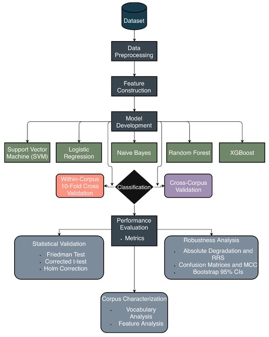
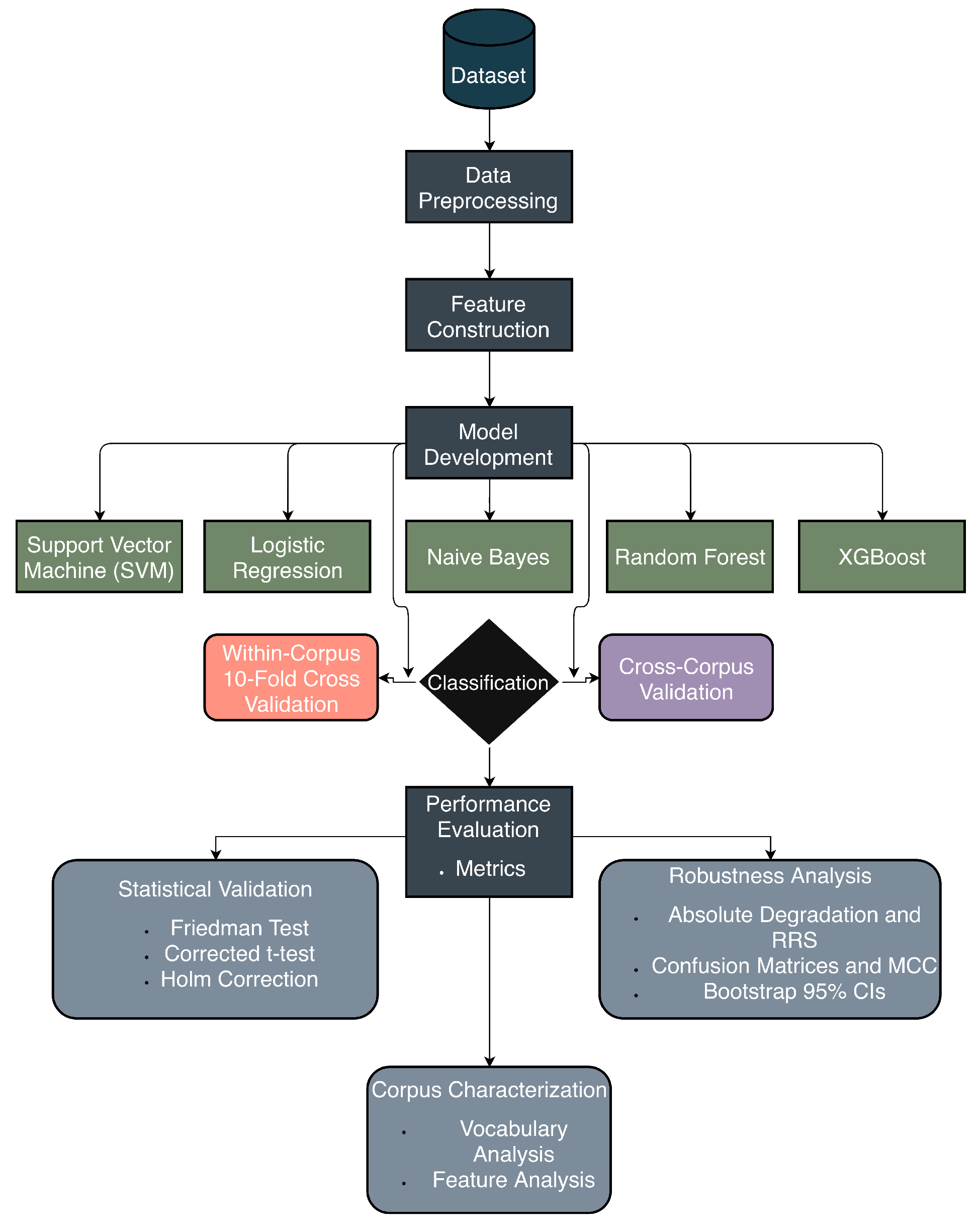
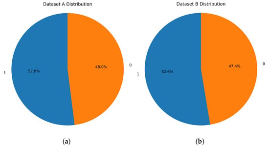
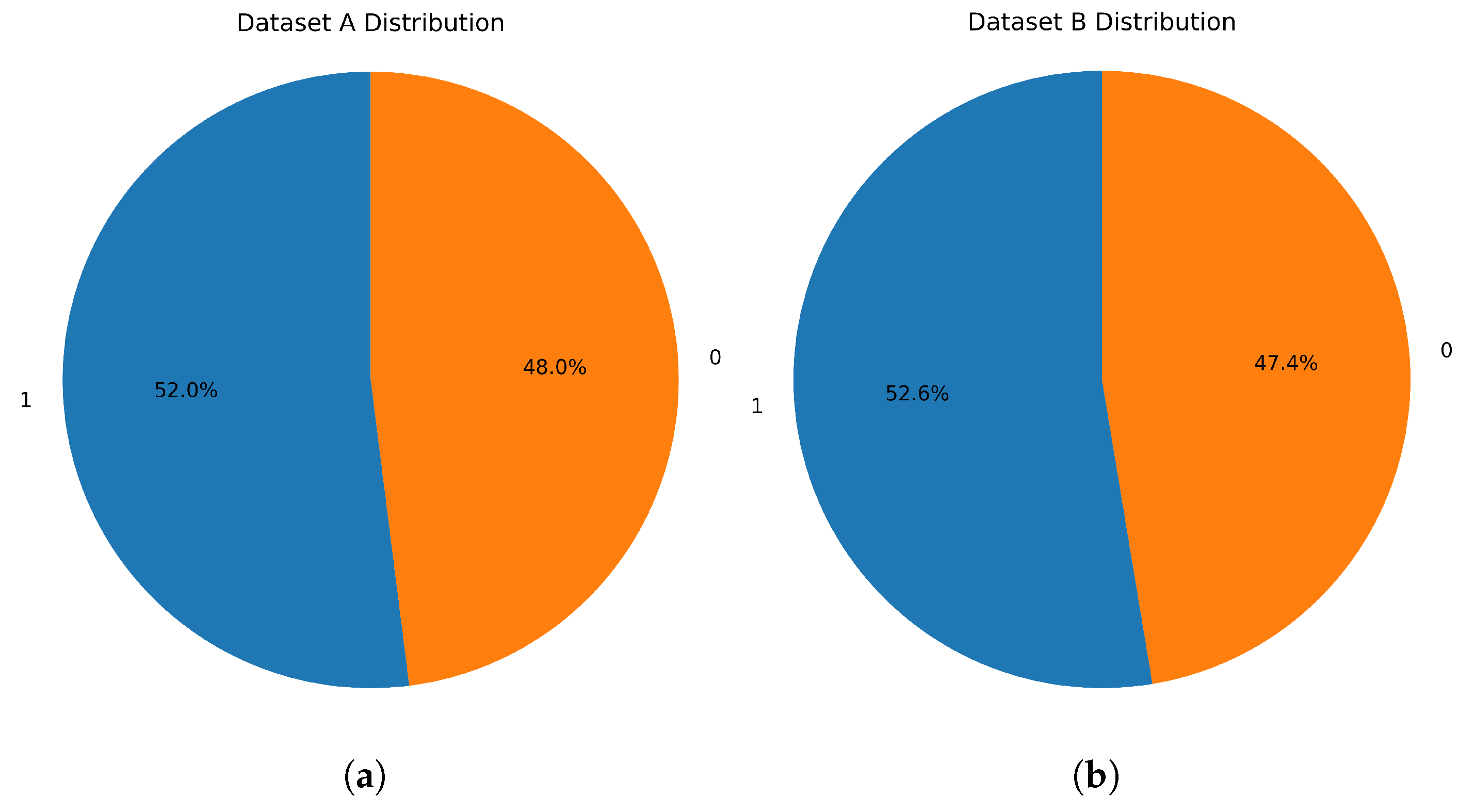
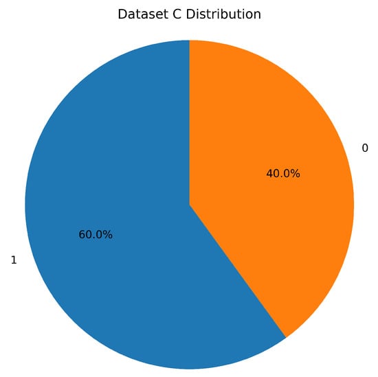
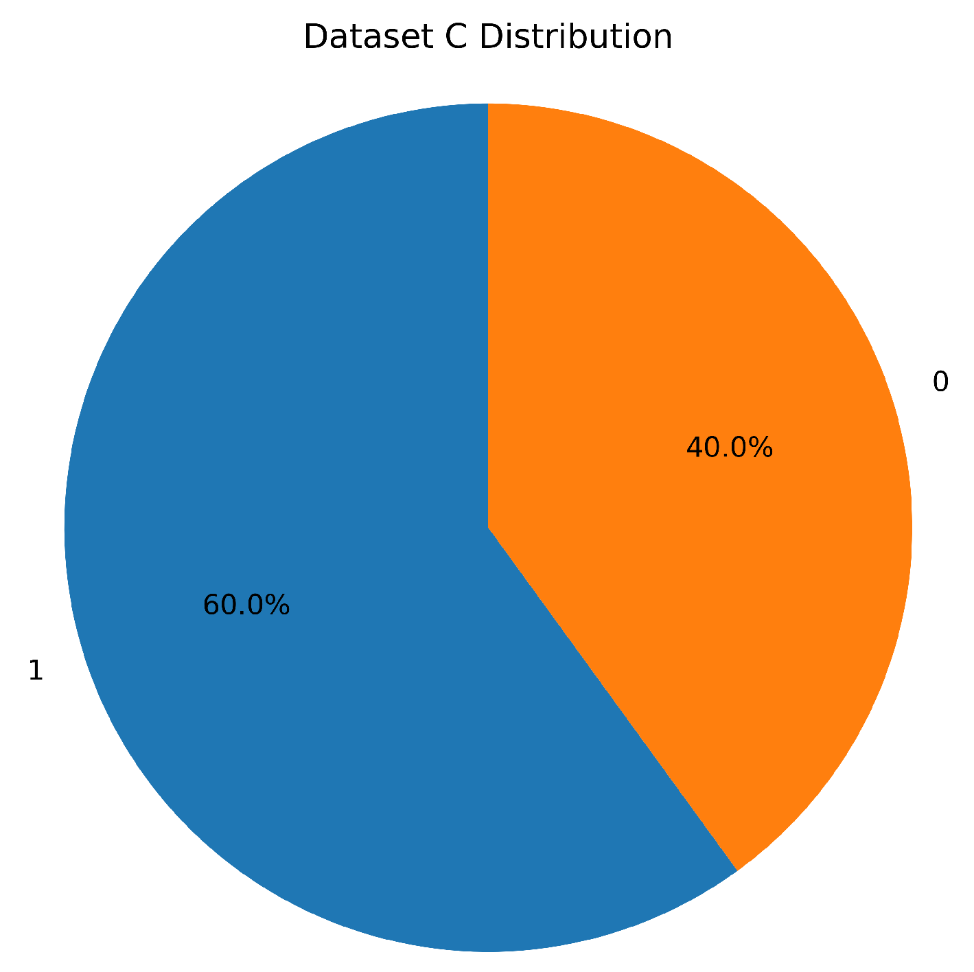
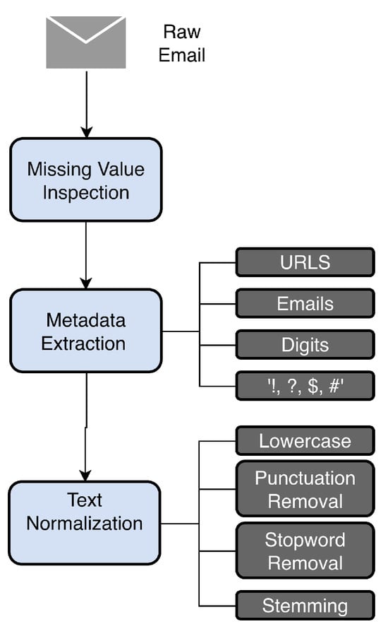
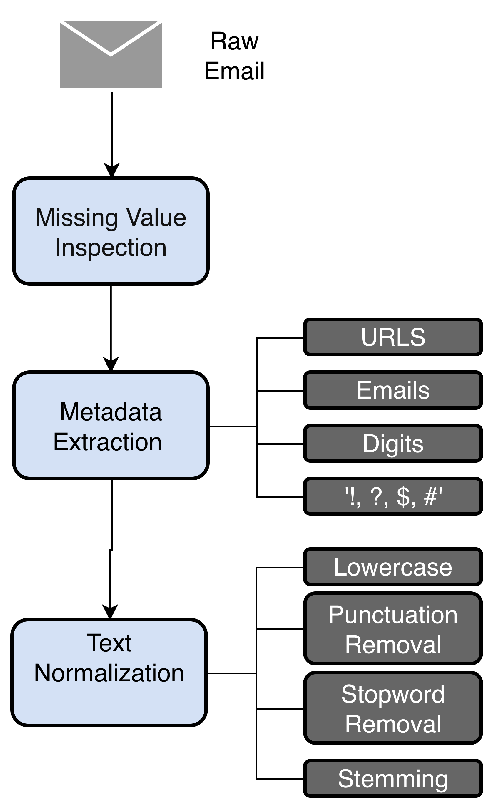
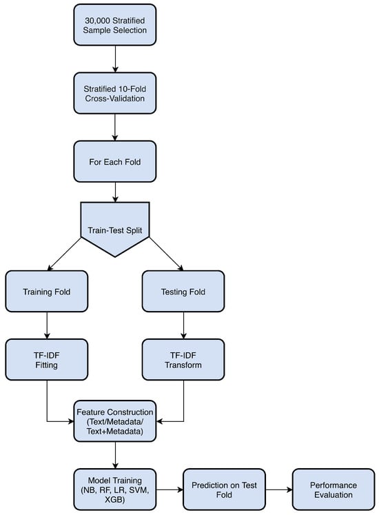
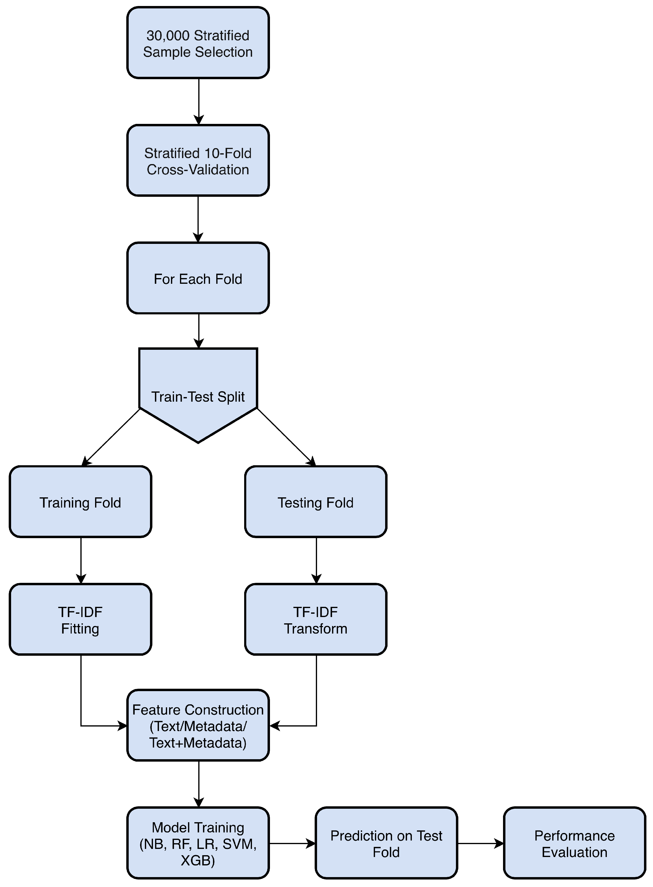
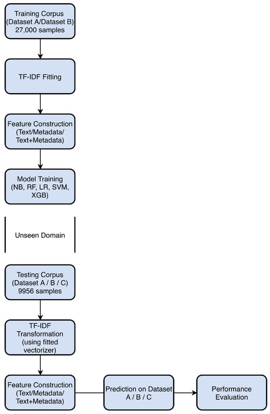
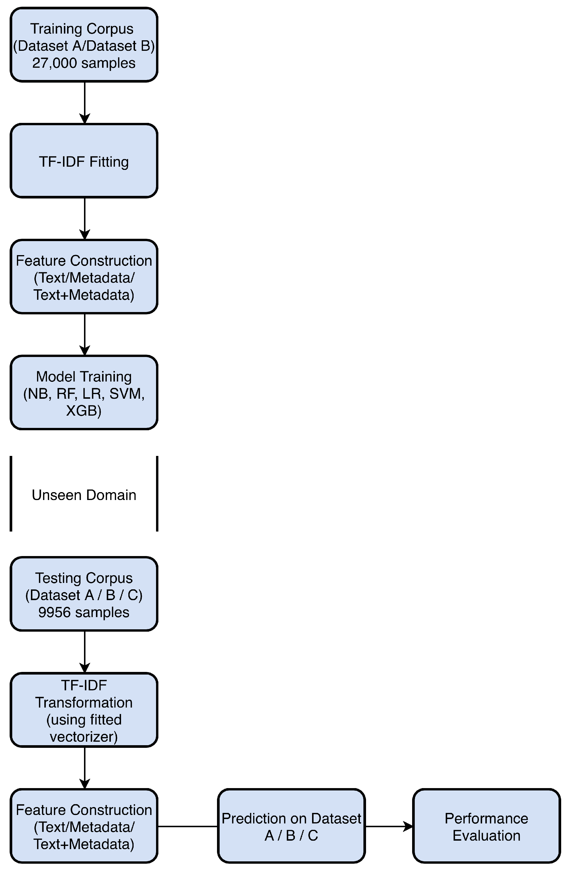
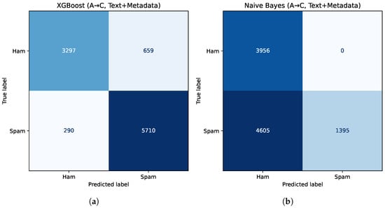
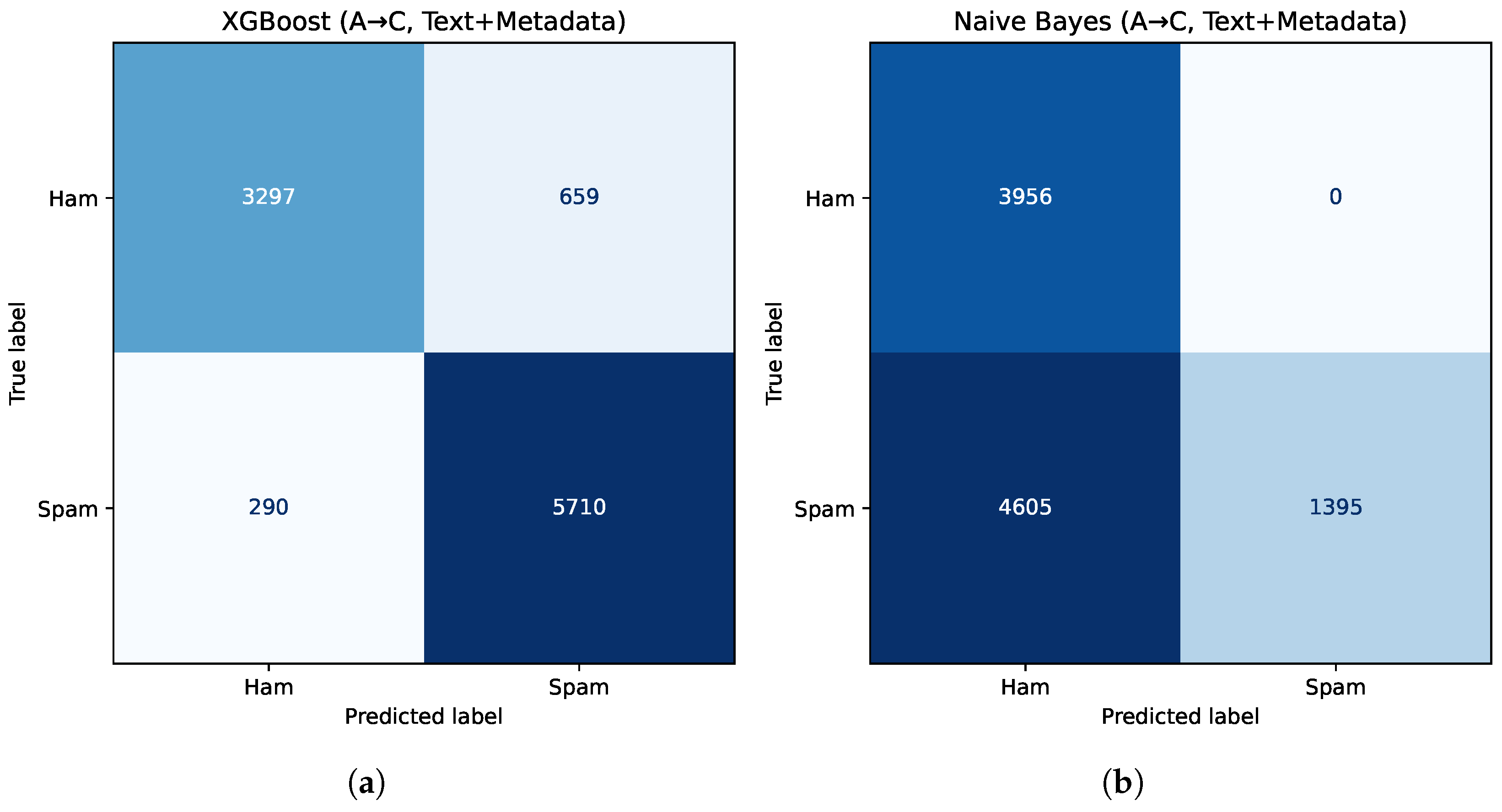
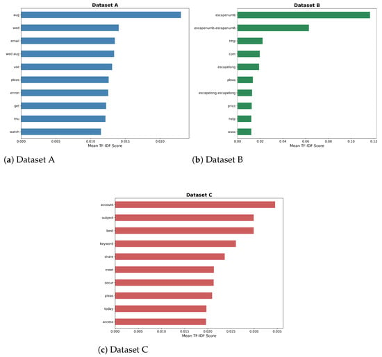
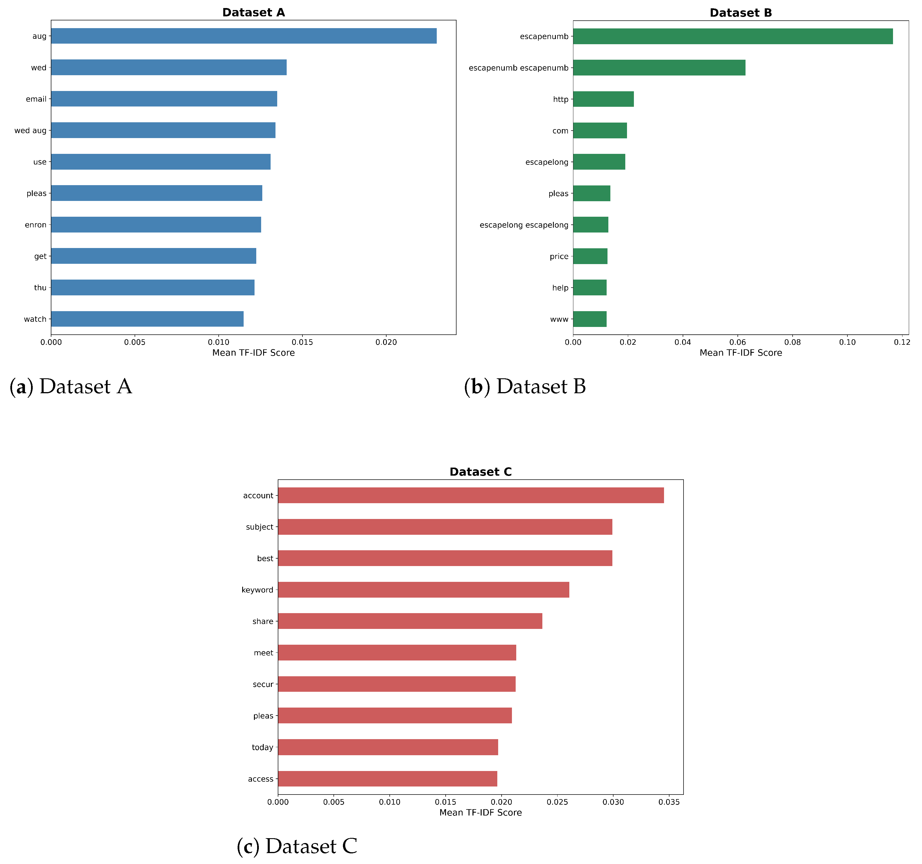
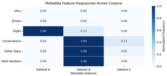

Disclaimer/Publisher’s Note: The statements, opinions and data contained in all publications are solely those of the individual author(s) and contributor(s) and not of MDPI and/or the editor(s). MDPI and/or the editor(s) disclaim responsibility for any injury to people or property resulting from any ideas, methods, instructions or products referred to in the content. |
© 2026 by the authors. Licensee MDPI, Basel, Switzerland. This article is an open access article distributed under the terms and conditions of the Creative Commons Attribution (CC BY) license.