


Abstract
Short-circuit-ratio-type indices describe the static fault level of a connection point but not how much network weakening, dispatch growth, or control-parameter drift a heterogeneous multiport system can absorb before a damping threshold or a stability limit is reached. This paper defines a dynamic system strength for systems with grid-following, grid-forming, modular multilevel converter, and synchronous-machine ports. The device–network return-difference matrix is normalized based on a power metric built from rated powers and port bases, which makes its frequency-band margin invariant to port units, base values, and power-preserving coordinate transformations. Network, dispatch, control, and model-uncertainty stresses form structured blocks, and dynamic strength is the largest multiplier of a task-specific stress set inside a safe set defined jointly by stability, performance thresholds, and an applicability flag. A first-boundary tracking algorithm with candidate-band refinement from eigenvalues or from frequency data alone reports radius bounds, the critical frequency, and the active failure mechanism, and radius changes are allocated completely to continuous and discrete resources based on Aumann–Shapley and Shapley values. On a three-port benchmark, three support resources raise the performance radius from 0.4884 to 1.4012 at an unchanged static proxy, and the normalized margin is unchanged under base changes with condition numbers up to 1000, whereas the raw singular value drifts by up to two orders of magnitude. On a converter-level test system with converters rated 1000, 100, and 10 MVA, the first boundaries are a return-difference threshold in the PLL–network band and the transfer limit of the weakened network, the allocation credits the PLL retuning of the large plant with 87% of the radius change and a non-binding damping resource with zero, and the applicability flag withholds the small-signal statement when the current limiters engage.
1. Introduction
1.1. Motivation
Power systems that combine grid-following (GFL) converters, grid-forming (GFM) converters, modular multilevel converter (MMC)-based high-voltage direct current (HVDC) links, synchronous generators, and synchronous condensers are planned and operated with an imbalance between the quantities that are routinely computed and the phenomena that actually limit operation. The static fault level of a connection point is easy to compute and easy to compare across projects, and short-circuit-ratio (SCR) type indices have therefore become the default measure of “grid strength” in interconnection studies. The stability phenomena that actually limit such systems, however, are dynamic: the revised classification of power system stability introduced converter-driven and resonance stability precisely because phase-locked loops, inner current loops, DC-voltage loops, and virtual-synchronous controls interact with the network impedance at frequencies from a few hertz to several hundred hertz [1], and GFL and GFM converters respond to a weak network in opposite directions [2,3], so that the same static fault level can host very different dynamic outcomes.
Field experience confirms the mismatch between static and dynamic strength. Sub-synchronous interaction between direct-drive wind farms and a weak AC network was traced to converter–network coupling rather than to an inadequate fault level [4], and sub-synchronous resonance in wind farms behind series compensation depended on the number of turbines online, wind speed, and control settings [5]. In such cases the operator needs answers that a static index cannot provide: how much further can the network be weakened, how many megawatts can be added, how far can a control gain drift before the first damping or stability limit is met, which frequency and which port pattern will fail first, and which devices, set-points, and connection points contribute to or consume the available margin. This paper defines and computes a dynamic system strength that answers these questions for heterogeneous multiport systems and, equally importantly, states when the answer cannot be given by a small-signal model.
1.2. Existing Approaches and the Remaining Research Gap
Two families of methods dominate the literature. The first family extends the SCR concept after the single-converter studies of weak-grid instability [6,7]: Wu et al. defined a site-dependent SCR that captures interactions among several renewable plants through power-flow sensitivities [8]. Zhang et al. proposed the generalized SCR (gSCR) for multi-infeed LCC-HVDC systems by decoupling the network into equivalent single-infeed systems [9], Dong et al. extended the gSCR to multi-infeed VSC systems of homogeneous converters [10], and Henderson et al. embedded frequency-dependent converter impedances into a grid-strength impedance metric evaluated at each connection point [11]. They either contain no converter dynamics at all or assume identical converters, they evaluate one connection point at a time, and they return a single number without a frequency, a failing port pattern, or an engineering tolerance in ohms, megawatts, or control units.
The second family works directly with impedance or admittance models. Sun formulated the impedance-ratio Nyquist criterion for a single inverter against a Thevenin grid [12], Wen et al. measured the two-by-two dq impedance of a grid-tied inverter and exposed the negative q-axis resistance produced by the phase-locked loop [13], Rygg et al. proved the equivalence between the mirror-frequency-coupled sequence-domain impedance and the dq impedance [14], and Lyu et al. applied harmonic linearization to MMC-HVDC with a wind farm [15]. Liu et al. built a unified dq-frame impedance network for a whole system and derived an oscillatory-stability criterion from the determinant of the nodal admittance matrix [16], and Zhang et al. compared loop-gain, determinant-based, and eigenvalue-based criteria on impedance networks and exposed their partition dependence and hidden right-half-plane-pole pitfalls [17]; passivity [18] and harmonic-stability [19] assessments complete this family. These methods answer “is the present operating point stable” and “how far is a given frequency from singularity”, but they do not define a set of physically structured stresses, do not normalize heterogeneous ports so that a singular value has a coordinate-independent meaning, and do not distribute a finite margin change to several continuous or discrete resources.
Converter-level studies in the power-electronics literature refine the device side of the same problem. Jiang et al. built a small-signal model of a system supplied entirely by converters and determined the smallest share of grid-forming converters that keeps it stable [20], Wang et al. mapped the stable, unstable, and physically infeasible operating regions of a grid-forming direct-drive wind turbine over its continuous operating space [21], Chen et al. identified the weakly damped modes of a heterogeneous grid-following photovoltaic and grid-forming storage system under a low short-circuit ratio and tuned the coupled parameters to restore damping [22], and Gebremedhin derived reduced-order converter models to assess remote converter interactions [23]. Each of them, however, evaluates one converter family, one control design, or one network strength at a time, and none returns the admissible stress along a task direction together with the mechanism that fails first and the allocation of the margin among resources.
Robust-control tools close part of the distance. The complex structured singular value quantifies the smallest structured perturbation that destroys stability [24], and Djukanovic et al. cast operating-point variations of multimachine systems as structured uncertainty for robust stability analysis [25]; modal analysis supplies the inter-area modes [26], participation factors [27], loading-margin sensitivities [28], and ringdown identification [29]. Fair allocation of a shared quantity has a long record in power systems, mostly for costs and losses: Junqueira et al. applied the Aumann–Shapley scheme to the transmission service cost [30], and Molina et al. combined circuit theory with Aumann–Shapley allocation for complex losses [31]. None of these works allocates a dynamic margin to devices, set-points, and connection points with a completeness guarantee. Finally, small-signal conclusions have a limited domain of validity: current saturation can remove the stable equilibrium of a droop-controlled converter [32], and grid-forming current-limiting strategies change the equilibrium structure and transient behavior [33]. The frozen operating state on which any small-signal quantity is computed is one sample of a scenario space, and dedicated scenario-generation methods supply long-term renewable-generation scenario sets for that purpose [34],; the strength quantity of this paper is evaluated once per scenario of such a set, which is why its cost per evaluation is measured in Section 3.10.
Nonlinear control design complements these linear tools with estimates of the region in which a controlled nonlinear system returns to its equilibrium. An intermittent controller for uncertain nonlinear systems with an adjustable function approximator and a Lyapunov stability proof [35] and its data-driven successor with a Lyapunov-guided estimate of the attraction region [36] are examples. Such attraction-region estimates describe how large a disturbance a nonlinear closed loop survives, which is the question that the applicability flag of Section 2.3.6 hands over to the time-domain evaluation.
The practical gap is therefore not the absence of stability criteria. It is the absence of a strength quantity that (i) is defined on the physical stress space of network weakening, dispatch growth, control drift, and model uncertainty rather than on an unstructured norm; (ii) is invariant to port units, base values, and power-preserving coordinate transformations for the dq, sequence and AC/DC ports; (iii) returns the first boundary along a task direction with an interval, a critical frequency, a critical port direction, and the mechanism that fails first, including the case in which the dominant mode switches; (iv) allocates the finite change of that boundary completely to continuous and discrete resources and reports their interactions; and (v) refuses to issue a physical stability statement when limiters, blocking, mode switching, or model confidence invalidate the small-signal model.
1.3. Contributions and Paper Organization
The first contribution is a definition of dynamic system strength as a structured safe stress set and its task-direction radii. The safe set is the intersection of internal stability, well-posedness, closed-loop stability, performance thresholds, and an applicability condition, evaluated on the device–network return-difference matrix after power-metric normalization. The frequency-band return-difference margin obtained in this way is invariant to power-preserving coordinate transformations, which include port re-ordering and base changes as special cases.
The second contribution is a first-boundary tracking algorithm that combines adaptive continuation along a stress direction, joint stability and performance criteria, candidate-band frequency refinement, safe–unsafe interval contraction, and mode tracking through singular-vector continuity and that reports radius bounds, the physical tolerance, the critical frequency and port direction, and the active failure mechanism, with Clarke generalized gradients where the active mode switches. Two safeguards complete the algorithm: a slack-bounded continuation step, derived from the eigenvalue-sensitivity bound, which cannot step over a narrow unsafe region and counts every transition along the direction, and a candidate-band construction that needs no state-space model, in which the candidate frequencies come from a rational fit of the sampled closed-loop response and from the phase increments of the determinant of the return difference between consecutive grid points.
The third contribution is a complete contribution allocation. Continuous resources receive Aumann–Shapley path-integral contributions whose sum equals the radius change along any admissible path, discrete resources receive exact or sampled Shapley values, pairwise interaction indices separate synergy from antagonism, and the device capability, set-point, and connection location are treated as distinct resource axes.
The fourth contribution is a reproducible three-port constructed benchmark and a converter-level test system with detailed grid-following and grid-forming converter models whose ratings span 10 MVA to 1000 MVA, on which every step of the chain is exercised and audited, including a quantitative comparison with static, impedance-based, modal, and unstructured margins, the sensitivity of the radii to thresholds and reference scales, the path dependence of the allocation, and the behavior of the applicability flag against converter current limiters.
2. Materials and Methods
Section 2.1 establishes the multiport return-difference model, Section 2.2 turns it into a strength quantity, Section 2.3 gives the algorithms that compute it, and Section 2.4 describes the benchmark and Section 2.5 the converter-level test system.
2.1. Multiport Return-Difference Model and the Limits of Static Indices
2.1.1. Port Relations and the Return-Difference Matrix
In a frozen operating state described by the parameter vector , every device is represented by a small-signal admittance from its port voltage increments to its port current increments. Stacking all device ports gives the following device relation:
where and are the stacked port current and voltage increments, is the block-structured device admittance matrix that collects GFL, GFM, MMC, synchronous-machine, and condenser ports, and is the Laplace variable. A dq port occupies two coordinates, a sequence-domain frequency-coupled port occupies two coordinates at mirrored frequencies, and an MMC AC/DC port occupies the AC coordinates plus one DC coordinate. The network seen from the same ports satisfies the following:
where is the multiport network impedance matrix and is the source-side voltage disturbance. Combining Equations (1) and (2) gives the closed-loop relation between the disturbance and response:
where is the dimensionless return-difference matrix. If is singular at some real frequency, a non-zero port-voltage pattern reproduces itself after one pass through the device response and the network feedback, and no external excitation is needed—the system is at a small-signal stability boundary at that frequency. When the open-loop subsystems have no hidden unstable modes, the closed-loop characteristic polynomial and the open-loop polynomials and are related through the determinant of the return difference:
which is the identity used by the generalized Nyquist criterion and which links the frequency–domain object of Equation (3) to the state-space eigenvalues used later as a cross-check.
2.1.2. Functional Dependence and Omissions of Static Strength Indices
Every SCR-type index is a function of the fundamental-frequency network matrix and of rated powers only. In the notation of Equation (2), this family can be written as follows:
where is the fundamental angular frequency and collects the rated powers. The classical SCR is the ratio of the short-circuit capacity to the rated power at a single port; the gSCR is the smallest eigenvalue of a capacity-normalized network matrix. Equation (5) makes the two omissions explicit. First, does not appear: the phase-locked-loop bandwidth, the current-loop and DC-voltage-loop gains, the virtual inertia and damping of a GFM converter, and the internal dynamics of an MMC leave unchanged, although each of them changes in Equation (3). Second, only appears: the network is characterized at 50 or 60 Hz, whereas converter–network interactions occur at the frequencies where a device admittance shows a negative real part and the network reactance resonates with it. Section 3.5 quantifies these omissions based on the benchmark by holding and hence fixed while changing only device-side support.
2.1.3. Coordinate Dependence of the Raw Minimum Singular Value
The natural frequency–domain distance from Equation (3) to singularity is the minimum singular value of . Its value, however, depends on how lengths are measured in the stacked port space. Under an invertible change of port coordinates , the return difference transforms by similarity:
where is a positive scalar. Eigenvalues are similarity invariants, but singular values are not: a change in the voltage base of one port, a change in units, or a mixing of AC and DC coordinates changes , while the physical system is unchanged. Equation (6) is the reason why a metric has to be chosen before a singular value can be called a strength; Section 2.2.1 chooses the metric so that the resulting margin measures perturbations by the power that they represent.
The size of the drift is bounded by the conditioning of the coordinate change. The smallest singular value of a product is at least the product of the smallest singular values of the factors; applying this inequality to and to gives the following:
where is the condition number of the coordinate change. For a diagonal base change it is the ratio of the largest to the smallest base factor, so a port set whose voltage bases span 500 kV to 35 kV admits a drift of up to 14.3 between the per-unit and the kilovolt description of the same loop, and a port set whose ratings span 10 MW to 1000 MW admits a drift of up to 100 between individual-base and common-base coordinates; Section 3.4 measures factors of 11.7 and 116 based on the benchmark for condition numbers 100 and 1000.
2.1.4. Modeling Requirements and Nomenclature
Devices and the network are represented as multiport blocks with a consistent port definition and known port bases. All later quantities are functions of the frozen state ; the operating point is not averaged over scenarios but evaluated per scenario. Physical stresses are always mapped to dimensionless coordinates through reference scales, so that ohms, megawatts, and control gains are never mixed in one norm. Table 1 lists the principal symbols.
Table 1.
Nomenclature and physical interpretation of the principal variables.
2.2. Dynamic Strength as a Structured Safe Stress Set
2.2.1. Power Metric and Normalized Return Difference
The metric is chosen so that the size of a port-voltage perturbation is measured based on the power that it represents. For port with rated apparent power , rated voltage , and coordinate dimension , the metric and the normalized return difference are as follows:
where is the identity of dimension and is the Hermitian square root of the positive definite metric. The quadratic form equals , so a one-percent voltage excursion on a 1000 MW port weighs ten times more than the same excursion on a 100 MW port. The weight is the rated admittance magnitude of port , so the quadratic form is the apparent power that the voltage perturbation would drive through the rated admittance of each port; this is what makes the metric independent of the converter technology behind the port, whose dynamics enter only through ; the d and q coordinates of a port share one weight, and the DC coordinate of an MMC port carries its own block with the rated DC power and voltage. The dual metric with the weights applies to current coordinates; it keeps the incremental power invariant and covers voltage-controlled ports, whose natural description is an impedance. The metric enters the safe set only through the return-difference criterion of Section 2.2.2.
The frequency-band margin is the infimum of the minimum singular value of the normalized return difference over the analysis band, which is the same as the minimum gain of measured in the metric norm:
where is the analysis band and ranges over non-zero port-voltage patterns. The minimizing is the critical port direction, and the minimizing is the critical frequency .
The margin defined in this way does not depend on the coordinates in which the ports are described, as long as the change in coordinates preserves incremental power. Let the port voltages be transformed by an invertible matrix , the port currents by the dual transformation that preserves the incremental power, and the metric accordingly:
where is the metric expressed in the new coordinates. Under this transformation, the device admittance becomes , the network impedance becomes , and the return difference transforms by similarity, . The two normalized return differences are connected by the matrix
which is unitary because the metric transforms contragrediently to the voltages, so that the transformed normalized return difference is a unitary similarity of the original one. Singular values are unchanged by unitary similarity, so and its critical frequency take the same values in both coordinate systems. Port re-ordering is the case of a permutation , and a change in base values is the case of a diagonal ; both leave unchanged, whereas Equation (6) shows that the raw changes under the diagonal case.
2.2.2. Joint Stability and Performance Criteria
The band margin alone does not decide closed-loop stability, because a system that is already unstable can show a large on the real frequency axis and because Equation (4) holds only in the absence of hidden unstable modes. The safe set therefore combines five criteria. Internal stability requires that every device block and the network block are stable on their own. Well-posedness requires that the interconnection has a unique solution, i.e., that is non-singular as . Closed-loop stability is checked in two independent ways whenever a full state-space model exists: by the generalized Nyquist count and by the eigenvalues of the closed-loop state matrix. The Nyquist count is written as follows:
where is the number of closed-loop poles in the open right half-plane, is the number of clockwise encirclements of the origin by as traverses the Nyquist contour, and is the number of open-loop right-half-plane poles. The eigenvalue check uses the modal damping ratio and the maximum real part of the eigenvalues:
where are the eigenvalues of the closed-loop state matrix. Closed-loop stability requires together with . The performance criterion requires , , and any user-defined constraint such as a settling-time or overvoltage limit. A mode with damping ratio decays to 5% of its initial amplitude in cycles, i.e., in 16 cycles at , in 11 cycles at , and in 10 cycles at ; the studies of this paper use 0.045, between the 3% that planning criteria commonly require for electromechanical modes and the 5% that stricter operating practices use. The return-difference threshold is a loop-robustness requirement: based on Equation (9), every metric-measured loop perturbation of norm below leaves non-singular on the whole band, so guarantees a 5.5% loop margin against modeling error in the critical band. Section 3.12 reports the sensitivity of the radii to both thresholds. The applicability criterion is the flag defined in Section 2.3.6. Whenever the boundary search of Section 2.3.1 leaves the safe set, the criterion that fails first is recorded as the active failure mechanism, so that a violation of the damping threshold is never reported as a loss of stability.
2.2.3. Structured Physical Stresses
Line impedances, dispatched active and reactive powers, phase-locked-loop and GFM control parameters, MMC control parameters, and uncertain model parameters have different units. Each physical parameter is standardized by its reference value and a non-zero reference scale:
where is the value at the reference state, has the unit of , and the dimensionless stress vector is partitioned into a network-weakening block , a dispatch block , a control block , and a model-uncertainty block . Each block enters the model at its physical location: modifies , and modify the operating point and the controllers inside , and perturbs identified or vendor parameters within their confidence ranges.
The reference scales are part of the task definition, and two properties govern their choice. First, along a task that is specified in physical units—a given line, a given plant, and a given controller—the physical tolerance of Equation (18) does not depend on the scale: replacing by divides the dimensionless radius by and multiplies the recovered tolerance by , so the tolerance is unchanged. Second, along a task that mixes several blocks in dimensionless coordinates, such as the combined direction of the benchmark, the scales fix the relative weight of the blocks and therefore the physical direction; two analysts who use different scales follow different physical paths and obtain different radii, so the scales are chosen so that one unit of each block is comparably plausible (the most severe single outage, the rated power of the plant, and the tolerance band of the vendor data). Section 3.12 quantifies both properties based on the benchmark.
The parameter vector at a stress is as follows:
where selects the position of parameter in . Because the stresses keep the structure of the physical model, the resulting perturbation of is structured; an unstructured matrix perturbation of the same norm would correspond to no realizable network or dispatch change.
2.2.4. Safe Stress Set and Directional Strength Radius
The safe stress set at a reference state collects the standardized stresses under which all five criteria hold:
where the product of 0/1 indicators is the logical conjunction, and the arguments of to are the same as that of . The criteria are parallel members of an intersection; they are not weighted and summed. For a task a, unit stress set is specified as a direction or a compact set in stress space, and the directional strength radius is the largest multiplier that keeps the scaled task set inside the safe set:
where is the dimensionless stress multiplier. The physical tolerance follows by inverting Equation (14) along the task direction:
where is the -th component of the unit stress direction of task . Because the safe set is defined per operating state and per threshold set, the radius is state-dependent by construction, and a stability radius obtained by dropping from Equation (16) separates the pure stability limit from the performance limit.
2.2.5. Ordering of Operating States and Relation to Static Indices
Two operating states are compared first by set inclusion and only afterwards by radii:
which is a partial order: when neither safe set contains the other, no weight-free global ranking exists, and the radii along the task directions of interest are reported side by side instead of being merged into one score. Static indices fit into this picture as one-dimensional projections. When every device is a homogeneous GFL converter, the network is inductive, and the band is restricted to the quasi-static low-frequency range, the network-weakening block of Equation (14) acts on the fundamental-frequency network matrix only and the radius along a proportional network-weakening direction is a monotone function of the smallest eigenvalue of the capacity-normalized network matrix, which is the gSCR.
2.3. Boundary Tracking, Contribution Allocation, and Applicability Screening
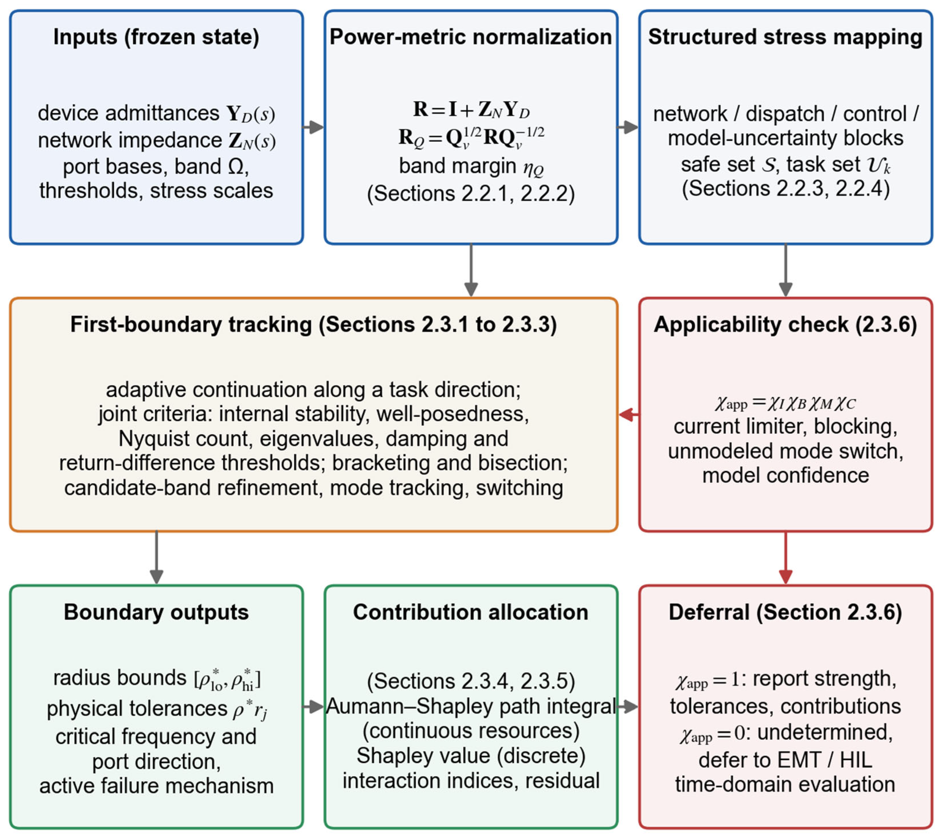
Figure 1 summarizes the chain from inputs to outputs.
2.3.1. First-Boundary Tracking Along a Task Direction
Starting from the safe reference point , the multiplier is increased with an adaptive step. Each candidate point is evaluated in a fixed order: internal stability and well-posedness first, then the band margin of Equation (9) based on the candidate frequency set, then the Nyquist count of Equation (12) and the eigenvalue quantities of Equation (13), and finally the performance thresholds. The multiplier update is as follows:
where is the expansion factor, and the search stops expanding as soon as the first unsafe candidate is met. When the safe set is not known to be star-shaped, the step is bounded by the slack of every criterion divided by a bound on its derivative along the direction:
where is the slack of criterion (the distance of from zero, of from , and of from ), is a Lipschitz bound of over the step, and the second inequality, the eigenvalue-sensitivity bound with unit right and left eigenvectors and of the closed-loop state matrix , supplies for the eigenvalue criteria: the bound for is times the largest eigenvalue condition number, and the bound for follows by dividing by the modulus of the eigenvalue. With this rule, no slack can change sign between two consecutive safe candidates, so the first unsafe candidate is the first boundary; the same rule, continued past the first boundary up to a prescribed multiplier, counts every sign change of every slack and reports the number of transitions along the direction. Section 3.12 reports the cost and the transition counts on the benchmark.
Figure 1.
Method chain from the frozen operating state to the reported strength: power-metric normalization, structured stress mapping, first-boundary tracking under joint criteria, applicability check, contribution allocation, and deferral to time-domain evaluation.
The last safe point and the first unsafe point bracket the boundary, and the bracket is contracted by bisection or by a conservative secant step until its width falls below a tolerance:
where is the radius tolerance. The output is the interval, not a point, together with the criterion whose slack is smallest at , which is the active failure mechanism.
2.3.2. Candidate-Band Frequency Refinement and Mode Tracking
A lightly damped mode is a pole close to the imaginary axis, and along the frequency axis, it appears as a dip of whose depth and half-power width are both proportional to the distance of the pole from the axis, i.e., to . The most dangerous dips are therefore also the narrowest, and a fixed frequency grid can step over them. Instead of a single global minimum, the algorithm collects every interior local minimum of the grid curve as a candidate and refines each candidate on its bracketing interval:
where is the set of grid indices at which the grid curve has a local minimum and the inner minimization is carried out by a golden-section search. Refining only the global grid minimum is not sufficient, because a coarse grid can place its global minimum in the wrong dip; Section 3.3 shows both failure modes based on the benchmark.
The candidate set does not require a state-space model. When the ports are described by measured or identified frequency responses, the modal frequencies are recovered from the sampled closed-loop response itself: the inverse return difference on the coarse grid is fitted by a rational function with common poles,
where are the fitted poles, the residue matrices, the constant term, and the fit order; the poles are relocated iteratively based on the vector-fitting algorithm [37], and the imaginary parts of the fitted poles form the candidate set . A second detector uses only the phase of the sampled determinant, whose zeros are the closed-loop poles: a zero close to the imaginary axis turns the phase of by about within a frequency interval whose width is the real part of the pole, so the phase increment between consecutive grid points,
marks every interval that contains a dip narrower than the grid, whether or not the magnitude shows a local minimum there; is used. Section 3.3 reports both generators based on the benchmark next to the eigenvalue-guided refinement.
Mode identity across consecutive stress points is tracked through the continuity of the critical singular vector and, when a state-space model exists, of the eigenvector, using the overlap index:
where is the unit critical port direction. A drop in below a threshold or a change in the criterion with the smallest slack marks a switch of the active mode or of the active constraint, and the switch point is stored with the boundary.
2.3.3. Local Sensitivity of the Radius and Non-Smooth Switching
When a single active constraint is smooth at the boundary, the radius is defined implicitly by the active boundary function —for example —and its sensitivity to a continuous resource follows from the implicit-function theorem:
where the partial derivatives are evaluated at and can be obtained from eigenvalue sensitivities or from finite differences of . Equation (27) gives, without a second boundary search, the local increase or decrease in the admissible stress multiplier per unit of the resource. When two active modes or two active constraints exchange roles at the boundary, the derivative is not unique, and the algorithm reports one-sided derivatives, the Clarke generalized gradient, or a contribution interval:
where is the gradient computed with active mode or constraint alone and is the active set. Forced smoothing of the switch is avoided because it would hide the mode change from the operator.
2.3.4. Aumann–Shapley Allocation for Continuous Resources
Let and be a physically admissible reference and current resource state, and let the straight path between them stay inside the domain on which is defined and differentiable almost everywhere. The Aumann–Shapley contribution of resource integrates its local marginal effect along the path:
where is the path parameter. Because the integrand is the directional derivative of along the path, the gradient theorem gives the completeness identity:
where is the number of continuous resources. Equation (30) is the auditable property that single-point sensitivities lack: the contributions sum exactly to the finite radius change, so an omitted or double-counted resource shows up as a non-zero residual.
Completeness holds along every admissible path, but the division of the total among the resources does not: the contribution of resource along a path is , and for two paths and with the same end points, the difference between the two contributions of resource is the circulation of around the closed loop formed by the paths, which Green’s theorem turns into an integral of the cross-sensitivities over the region between them:
where is the region enclosed by the projections of the two paths on the plane. The straight path is therefore a modeling choice; it is the choice singled out by the Aumann–Shapley axioms, and the sequential orders of a what-if study are the extreme paths that run along the coordinate axes, whose spread is exactly the interaction between the resources. For resources switched in at their current level, the credit of resource when it is switched last minus its credit when it is switched first equals the sum of its pairwise interaction indices of Equation (35) and the three-way remainder, which Section 3.6 verifies to machine precision.
The integral is evaluated by midpoint quadrature with central differences of the radius:
where is the number of quadrature points and the finite-difference step, so that each contribution costs boundary searches. If the straight path crosses an unstable region, a piecewise-linear dispatch path or several admissible paths are used and reported; a path that crosses instability is never used as the only attribution path.
2.3.5. Shapley Allocation for Discrete Resources and Interaction Indices
Lines, units, and control modes are switched in or out rather than varied continuously. With denoting the directional radius when only the resources in coalition are in service, the Shapley contribution of resource is the fairly weighted average of its marginal effect over all coalitions:
where is the coalition size and the number of discrete resources. The efficiency axiom gives the discrete completeness identity:
which allocates exactly the difference between the all-in and the all-out radii. For small , the coalition values are enumerated; for large , random permutations are sampled and a confidence interval is attached. The interaction between two resources is measured based on the second-order difference in coalition values:
where a positive indicates synergy (the pair adds more together than separately) and a negative indicates antagonism. Device capability, set-point, and connection location enter the allocation as separate resource axes.
2.3.6. Applicability Flag and Deferral to Time-Domain Evaluation
Every small-signal statement is conditioned on the flag:
where if no converter current limiter is predicted to engage along the stress path, if no blocking or tripping threshold is reached, if no unmodeled control-mode switch occurs, and if the model confidence in the critical band is above its threshold. The limiter flag, for example, compares the predicted current excursion with the remaining headroom:
where is the pre-disturbance current of converter , the small-signal current excursion predicted for the design disturbance, and the limiter setting. When , the radius bounds, the physical tolerances, the critical frequency and port direction, the active mechanism, and the allocations are reported. When , no physical stability statement is issued; the output is “applicability failed” or “undetermined—defer to electromagnetic-transient (EMT) or hardware-in-the-loop (HIL) evaluation”—and the case is added to the set of scenarios that require such detailed time-domain study. Section 3.9 exercises the flag based on the benchmark with a limiter that saturates the support force of the resources, and Section 3.13 exercises it based on the converter-level test system against converter current limiters.
2.4. Benchmark Design and Evaluation Procedure
2.4.1. Purpose and Evidence Boundary
The benchmark is a constructed small-signal system with three coupled ports. It is not field data, not a vendor model, and not an electromagnetic-transient model; its role is to show that every step of the chain executes, that the outputs are reproducible to the stated tolerances, and that the mechanisms discussed in Section 2.1, Section 2.2 and Section 2.3 are visible in numbers.
2.4.2. Constructed Three-Port Model
The benchmark uses three second-order coupled ports whose generalized states are normalized small-signal deviations at a GFL-type equivalent, a GFM-type equivalent, and an MMC AC/DC equivalent port, with the closed-loop state matrix
where is the diagonal normalized inertia matrix, the restoring-coefficient matrix in , the damping-coefficient matrix in , the structured stress multiplier, and the continuous resource state; the restoring and damping matrices are sums of a network block and a device block with their own stresses and support terms:
and the damping matrix follows the same composition:
where and are the network-weakening and device-stress multipliers, the subscripts w and s mark the weakening and stress patterns, and and are the diagonal support patterns of the three resources shown in Figure 2. The same matrices define the frequency–domain blocks of Section 2.1, so that the eigenvalue check and the return-difference margin are computed based on one model:
Figure 2.
Constructed three-port benchmark: (a) three coupled ports, the network block subject to network weakening, the device block subject to device stress and to the three support resources, and the return difference that links them; (b) diagonal support weights of the three resources based on the restoring (left) and damping (right) coefficients of the three ports, with the GFM virtual damping, the synchronous-condenser support, and the MMC supplementary damping; the color scale of (b) runs from white at zero to dark blue at 0.45 ( for the restoring and for the damping weights), so that darker cells are larger weights, and each cell is labeled with its value.
Table 2 lists the complete parameter set; the coupling matrix is a Laplacian-type pattern that couples the three ports.
Table 2.
Parameter set of the constructed three-port benchmark (all matrices 3 × 3; diag denotes a diagonal matrix; is the coupling pattern).
The device block has negative restoring and damping coefficients at the reference state, the constructed analog of the negative-resistance region of a converter admittance, and each support resource acts on all three ports with a dominant weight on its own port, so that the resources overlap and can interact.
2.4.3. Stress Directions, Resources, and Static Proxy
Three task directions are used. The combined direction scales the network-weakening and device-stress multipliers together, ; the network-only direction uses , and the device-only direction uses . The continuous resources are (GFM virtual damping), (synchronous-condenser support), and (MMC supplementary damping); the reference state is , the current state is , and a weakly supported control combination A with is used for the paired comparison. For the discrete allocation, the same three resources are switched in or out, either at unit level () or at their current level ().
Because the network block is identical for every resource state, any static index computed from the network alone takes the same value for every state. As a transparent proxy for such an index, the smallest eigenvalue of the network-restoring matrix is used:
which plays the role of a capacity-normalized network stiffness—the constructed analog of a generalized short-circuit ratio—and equals 9.5453 at for the reference state, the current state, and combination A alike.
2.4.4. Thresholds, Frequency Band, and Solver Settings
Table 3 collects the settings that determine every number in Section 3. The scripts, the models, and the exported trajectories are provided as Supplementary Code S1.
Table 3.
Solver, threshold, and procedure settings of the benchmark study.
2.5. Converter-Level Test System
The benchmark of Section 2.4 isolates the mechanisms based on a system that can be checked by hand. The test system of this section repeats the chain based on detailed converter models with physical ratings, a physical network, converter current limiters, and the mixture of current-controlled and voltage-controlled ports that a real multiport system contains. It is a small-signal and time-domain simulation study of a constructed system, not field data.
2.5.1. System and Converter Models
Three converter ports are connected through transformer-and-line branches to a point of common coupling (PCC) that is tied to an infinite bus through a Thevenin grid equivalent. Port 1 is a 1000 MVA grid-following plant connected at 500 kV, port 2 a 100 MVA grid-forming converter at 220 kV, and port 3 a 10 MVA grid-following cluster at 35 kV; the ratings span two orders of magnitude, which is the situation of Section 2.1.3 in which the raw singular value has no common scale. All quantities are per unit based on a common 100 MVA base with equal voltage bases behind ideal transformers, time is in seconds, and the model is written in a synchronous dq frame rotating at the nominal frequency.
The grid-following converters consist of an LC filter with a passive damping resistance in series with the capacitor, a synchronous-reference-frame PLL with a damping ratio 0.707 and bandwidth 40 Hz (port 1) or 25 Hz (port 3), active- and reactive-power set-points converted into current references through the measured terminal voltage, and a PI current controller with decoupling and terminal-voltage feed-forward tuned for a 300 Hz bandwidth based on internal-model control (, ); the DC voltage is assumed to be constant. The grid-forming converter has a virtual-synchronous active-power loop with an inertia constant of 2 s and a damping coefficient , a reactive-power/voltage droop of 5%, a 15 Hz power-measurement filter, and a virtual impedance of p.u. on its base through which the internal voltage drives the output current; the converter voltage is synthesized directly behind the virtual impedance, which assumes inner loops whose bandwidth lies far above the synchronization and virtual-impedance dynamics, and its filter inductor and damped filter capacitor are modeled explicitly. The reference dispatch is 600 MW and 100 Mvar at port 1, 30 MW at port 2, and 6 MW at port 3, and the grid equivalent gives a short-circuit ratio of 4.0 on the installed 1110 MVA at the PCC. Table 4 lists the parameters of the 34-state model. The equilibrium is solved via Newton iteration, the state matrix based on central differences of the nonlinear model, and the port blocks of Equation (3) based on the partition described next.
Table 4.
Parameters of the converter-level test system (own base: the rating of the port; system base: 100 MVA; rad/s).
2.5.2. Port Partition, Power Metric, Stresses, and Resources
Each device block receives its terminal voltage and returns its current, which is the admittance form of Equation (1); the network block, which contains the damped filter capacitors, the branches, the PCC capacitor, and the grid equivalent, receives the device currents and returns the terminal voltages. Because the terminal voltage includes the drop across the capacitor damping resistance, the network block has a direct feed-through term and the dependence of each device block on its own current through that term is assigned to the loop; the identity of Equation (4) then holds exactly, which is verified at the reference point by evaluating at the closed-loop eigenvalues (Section 3.13). A voltage-controlled converter with integral voltage control has an admittance block with right-half-plane poles, because its voltage controller acts on an exogenous voltage; such a port is described on its current coordinates with the dual metric of Section 2.2.1. The power metric is with the weights 1, 0.1, and 0.01, a spread of 100, and the kilovolt description is obtained with the diagonal of the connection voltages, whose condition number is 14.3.
Three physical stress blocks are used. Network weakening scales the grid inductance and resistance by , dispatch growth scales the active-power set-points of the two grid-following plants by , and control drift scales the PLL bandwidth of port 1 by . The combined direction is . The three resources separate the axes of Section 2.3.5: raises the grid-forming damping coefficient from 16 to 44 p.u. on its base (a control set-point), raises the grid-forming rating from 100 to 200 MVA with all of its per-unit quantities rescaled (device capability), and lowers the PLL bandwidth of port 1 from 40 Hz to 15 Hz (control retuning of the large plant). The reference state is , the current state , and combination A is , as on the benchmark.
2.5.3. Criteria, Limiters, and Procedure
The criteria are those of Section 2.2.2 with the thresholds of Table 3, the damping-ratio criterion applied to every oscillatory mode below 1 kHz, the analysis band 0.16 Hz to 1 kHz on a 360-point logarithmic grid, the internal stability of the device and network blocks, the existence of an equilibrium as the well-posedness criterion (its failure is the transfer limit of the weakened network), and steady-state converter currents within 1.1 times the rated current as the applicability condition at the operating point. The current limiters of the nonlinear simulations are a magnitude limit of 1.1 p.u. of the rated current based on the current references of the grid-following converters with priority on the active-power axis, and a threshold virtual impedance for the grid-forming converter whose virtual resistance and reactance grow by 1 and 4 p.u. based on its base per unit of relative excess current above the limit. The disturbance is a dip in the infinite-bus voltage of 2%, 5%, 15%, and 30% for 150 ms, applied at the current resource state at on the combined direction; the flag of Equation (37) compares the peak converter currents predicted by the linearized model with the limits, and the nonlinear model with limiters is integrated for 4 s. The allocation uses 12 midpoints and a step of 0.01.
3. Results
This section reports the results in the order of the method chain.
3.1. Directional Radii, Active Mechanisms, and Safe Sets
Table 5 lists the radii of the three resource states along the three directions with all criteria active (performance boundary) and with dropped (stability boundary).
Table 5.
Directional performance radii and stability radii of the three resource states along the three task directions (bisection tolerance ; interval widths between and ; 22 to 27 evaluations per boundary).
Three observations follow. First, the damping-ratio threshold is the active mechanism at every performance boundary, and the stability limit lies 15% to 109% further out; the method reports the two boundaries separately, so a violation of the 0.045 threshold is never confused with a loss of stability. Second, adding the three support resources multiplies the performance radius by 2.87 along the combined direction, 2.88 along the network-only direction, and 2.85 along the device-only direction, whereas the stability radius grows only by 1.90, 1.83, and 1.89: the resources act mainly on damping. Third, the two-dimensional safe sets of Figure 3 are nested— on the whole computed plane—so the partial order of Equation (19) is decisive here and the current state is stronger than the reference state in every direction.
Figure 3.
Two-dimensional safe stress sets in the plane of the network-weakening multiplier and the device-stress multiplier : (a) reference resource state; (b) current resource state. Green: all criteria satisfied; amber: stable but below the damping or return-difference threshold; red: unstable. Rays mark the combined, network-only, and device-only task directions with their performance radii (circles) and stability radii (squares).
The radii convert to physical tolerances. Along the combined direction, the network static proxy of Equation (42) falls from 9.5453 to 8.9366 (a 6.38% reduction) when the reference state reaches its performance boundary, to 7.7944 (18.34%) when the current state reaches its performance boundary, and to 7.1848 (24.73%) at the current stability boundary; expressed as a network tolerance, the same three support resources almost triple the admissible reduction in network stiffness before the damping threshold binds. On the 360-point grid, the trace does not reach zero at the stability boundary and oscillates between 0.02 and 0.06 beyond , the frequency-grid effect analyzed in Section 3.3.
3.2. Frequency-Resolved Margin, Mode Migration, and Active-Mode Switching
Figure 4 shows the frequency-resolved margin of the current state at four stress levels and the loci of the three oscillatory eigenvalue pairs as increases; Table 6 lists the three modes at the four boundaries of the combined direction.
Figure 4.
Frequency-resolved and modal view of the current state along the combined direction: (a) on the 360-point grid at , , , and ; (b) eigenvalue loci of the three oscillatory modes from (dots) to (arrow heads), with the constant-damping line and the modes at the performance boundary (circles) and at the stability boundary (squares).
Table 6.
Oscillatory modes at the performance and stability boundaries along the combined direction (modes ordered by frequency; the binding mode is marked; reference state at its performance boundary only).
The mode tracking reveals two facts that a scalar margin hides. First, the least-damped mode is not the same mode along the whole path: at the lowest-frequency mode 1 has the smallest damping ratio for both states, and mode 2 takes over at for the current state and at for the reference state; mode 2 is then the binding mode at every performance and stability boundary of the combined direction. Second, at the reference performance boundary, modes 1 and 2 have damping ratios of 0.0455 and 0.0450—a near-simultaneous activation of two constraints. In Figure 4a, the dip in the frequency-resolved margin deepens and narrows as grows and moves from 2.60 rad/s at to 2.89 rad/s at and 2.75 rad/s at , and at the stability boundary, the grid curve reaches only 0.038 although the true minimum is zero: the dip has become narrower than the grid spacing.
Both situations are what the overlap index of Equation (26) and the one-sided sensitivities of Section 2.3.3 are intended to handle, and both were exercised on the benchmark: the eigenvector overlap stays above 0.9999 inside every mode segment and collapses to 0.11 (current state) and 0.19 (reference state) at the step that spans the switch, which bisection then locates at 0.1680 and 0.4031, and the per-mode crossing radii at the reference boundary are 0.48843 (mode 2) and 0.49446 (mode 1), a gap of 0.0060. The mode-2-conditioned gradient of the radius, (0.5002, 0.4352, 0.3296), reproduces the local-linear estimate at the reference state reported in Section 3.6, while the mode-1-conditioned gradient is (0.2693, 0.4405, 0.7241). The GFM resource therefore improves the binding mode 2 almost twice as fast as it improves mode 1, and moving along the GFM-damping axis closes the 0.0060 gap already at . At that tie point, the one-sided derivatives of the radius along are 0.4998 from the left and 0.2694 from the right—each equal to its mode-conditioned slope to within —the Clarke interval of Equation (28) is their convex hull [0.269, 0.500], and a two-sided difference across the tie returns 0.3846, the mean of the two slopes and the derivative of neither active constraint.
3.3. Frequency-Grid Sensitivity and Candidate-Band Refinement
Table 7 quantifies the grid effect. The reference values are at 2.8875 rad/s, at 2.75423 rad/s (the imaginary part of the marginal eigenvalue in Table 6), and an -crossing radius of 1.79366.
Table 7.
Effect of the frequency grid and of the refinement strategy on the band margin and on the -crossing radius of the current state (combined direction; “none” means no crossing detected below ; evaluations refer to one margin evaluation at ).
The table shows both failure modes described in Section 2.3.2 and the remedy. Without refinement, the 30-point grid reports a margin of 0.306 at the stability boundary—five orders of magnitude above the true value—and never detects the crossing before the stability limit, and a 1440-point grid still reports 0.014, because the dip width vanishes as . Refining only the global grid minimum repairs the 30- and 360-point grids but not the 60-point grid: on that grid, the global minimum sits in the dip of mode 1 at 2.35 rad/s, the local search converges to 0.0488 at 2.36 rad/s, and the -crossing radius is overestimated by 4.6% (1.877 instead of 1.794). Refining all grid local minima does not help either, because the dip in the marginal mode 2 lies entirely between two grid points and creates no local minimum on the grid. Placing additional candidates at the eigenvalue frequencies—or, in continuation, at the previous critical frequency—recovers the correct margin, critical frequency, and crossing radius on every grid at a cost of 495 to 1011 single-frequency evaluations, i.e., less than three 360-point sweeps.
The modal information does not have to come from a state-space model. The two frequency-data-only generators of Section 2.3.2 reproduce the eigenvalue-guided result on every grid of Table 7. The rational fit of Equation (24) applied to the 30 sampled values of returns the three closed-loop pole pairs with imaginary parts 2.3652, 2.7542, and 3.1081 rad/s and the real part of the marginal pair to twelve digits, so that the candidates coincide with the eigenvalue frequencies without any eigenvalue computation; under 1% and 5% multiplicative noise on the samples, in all 80 trials, the candidate lies inside the grid interval that brackets the marginal frequency, which is all that the golden-section refinement needs. The phase screening of Equation (25) flags the interval from 2.68 to 3.07 rad/s on the 60-point grid, where the phase of turns by 114° between two consecutive samples, although the magnitude shows no local minimum there (Figure 5d), and recovers the margin at 2.7542 rad/s with 216 evaluations, fewer than the eigenvalue-guided refinement.
Figure 5.
Audits added on the benchmark: (a) ratio of the raw band minimum before and after diagonal base changes against the condition number of the base change, with the bound of Equation (7) and the unchanged metric margin; (b) normalized peak-to-peak envelopes of the port-1 generalized state over 500 s of simulation for the marginal scenario, the scenario with , and the scenario near the performance boundary of the current state, with the 14 s window of Section 3.8 shaded; (c) binding mode at the performance boundary and isolines of the radius over the resource plane at (blue: mode 2; red: mode 1), with the straight Aumann–Shapley path and the two extreme sequential paths; (d) of the current state at the stability boundary on a fine grid and on the 60-point grid, with the candidate frequencies from the rational fit of Equation (24) and the interval flagged by the phase screening of Equation (25).
3.4. Coordinate and Base Invariance
Table 8 reports the metric-normalized band margin and the raw minimum singular value at of the current state before and after four coordinate transformations applied according to Equation (10).
Table 8.
Invariance of the metric-normalized margin and drift of the raw minimum singular value under four coordinate transformations at of the current state (band minimum of the metric margin 0.447100 in all cases).
The metric margin is invariant to machine precision in every case, as the derivation of Section 2.2.1 requires; the base rescaling gives exactly zero difference because a diagonal commutes with the diagonal metric. The raw singular value changes by up to 0.16 at individual frequencies and its band minimum drifts by −8.70% under a mere change in base values.
The 8.70% of Table 8 is the mild end of the scale set by Equation (7), because the base change of that table has a condition number of only 4. Table 9 therefore applies diagonal base changes with condition numbers from 4 to 1000 to the same loop and assigns three rating realizations to the same return difference. Under the base changes, the metric margin moves by at most , whereas the raw band minimum falls by a factor of 1.96 at , the condition number of a port set at 500 kV, 220 kV, and 35 kV, by 11.7 at , and by 116 at ; the reversed rescaling with moves it by a factor of 21.4. The raw value in common-base coordinates is 0.4469 for every rating assignment, because the ratings do not enter it at all; the power-metric margin of a system whose ports are rated 1000, 100, and 10 MW is 0.288, that of the reversed assignment is 0.187, and the critical frequency moves from 2.96 to 2.65 rad/s between them. A raw singular value therefore overstates the physical margin of these two systems by factors of 1.55 and 2.39 and places the critical frequency on the wrong mode in the second case.
Table 9.
Drift of the raw band minimum under diagonal base changes of a growing condition number and band margin of one and the same loop under three rating realizations (current state, ; the metric margin before the base change is 0.4471 in every case).
3.5. Paired Comparison of Dynamic Radii at Identical Static Proxy
Combination A and the current state share every network-only quantity—, , the weakening blocks, and the static proxy —and differ only in the device-side support; Table 5 gives their radii.
The static proxy cannot distinguish the two combinations, while the dynamic performance radius differs by a factor of 2.19 in every direction and the stability radius by a factor of 1.61 to 1.65. Read as a network tolerance, combination A can lose 8.36% of its network stiffness before the damping threshold binds and the current state can lose 18.34%. This is the quantitative content of the argument in Section 2.1.2: the omission of from Equation (5) is not a small correction but a factor-of-two effect based on the admissible stress, and a planner who ranks connection options or control settings by a static index would rank these two combinations as equal.
3.6. Continuous Contribution Allocation
Table 10 gives the Aumann–Shapley contributions of the three resources to the change in the combined-direction performance radius from the reference to the current state, together with the single-point linear estimates at the two ends of the path, the sequential attributions in two switching orders, and the discrete Shapley values at current level.
Table 10.
Allocation of the performance-radius change along the combined direction to the three continuous resources (all values dimensionless; the last column is the sum minus relative to , in percent; GFM: virtual damping; Condenser: synchronous-condenser support; MMC: supplementary damping).
Four observations follow. First, the Aumann–Shapley contributions sum to the radius change with a residual of 0.0039%, and the residual stays below 0.021% for 2 to 48 midpoints and for steps from to . Second, the sequential attributions are strongly order-dependent: the GFM virtual damping is credited with 0.2216 when it is switched first and 0.4222 when it is switched last, and the MMC damping with 0.2302 or 0.4022 depending on the order, although every order sums to the same total. Third, the implicit-function sensitivity of Equation (27) agrees with the central-difference sensitivity to within (0.025%) at the current boundary, so the local sensitivities can be obtained from one eigenvalue-sensitivity evaluation instead of two boundary searches per resource once the active mode is known. Fourth, the Aumann–Shapley and the current-level Shapley allocations differ for the GFM and MMC resources (0.4071 versus 0.3224 and 0.2324 versus 0.3167) while agreeing for the condenser (0.2732 versus 0.2737): the two schemes answer different questions—gradual joint variation along the dispatch path versus all-or-nothing switching averaged over coalitions.
Table 11 quantifies the path dependence of Equation (31). Two curved admissible paths between the same end points, obtained by adding the deflection to the straight path, give the same total within the quadrature residual but divide it differently: the path that bends towards the GFM axis first () credits the GFM resource with 0.218 and the MMC resource with 0.408, almost exactly the sequential order in which the GFM resource is switched first, whereas the path that bends away from it () stays within 0.01 of the straight-path values. The reason is visible in Figure 5c, which maps the binding mode at the performance boundary over the plane at : mode 2 binds above a line that runs from the origin towards , mode 1 binds below it, and the gradient of the radius with respect to drops from 0.50 to 0.27 across that line (Section 3.2). The straight path stays on the mode-2 side, the first curved path and the sequential order with the GFM resource first cross into the mode-1 region, and this is where the GFM resource loses credit; the cross-sensitivity of Equation (31) is concentrated at that switching surface, and the 0.61% residual of the first curved path is the midpoint-rule error based on the kinked integrand. The identity of Section 2.3.4 holds to machine precision: the GFM credit when switched last minus its credit when switched first is , and ; for the MMC resource, the two sides are 0.1720 and 0.1720. The reference state matters less than the path: the shares from three reference states agree within 1.5 points with the same ranking.
Table 11.
Path dependence of the continuous allocation of (combined direction; 24 midpoints, ; shares in percent of the respective total in parentheses).
3.7. Discrete Shapley Allocation and Interactions
Table 12 lists the coalition values, the Shapley values, the pairwise interaction indices of Equation (35), and the three-way remainder for unit-level and current-level switching.
Table 12.
Discrete allocation of the combined-direction performance radius: coalition values , Shapley values, pairwise interactions, and three-way remainder for unit-level switching () and current-level switching ().
The efficiency identity of Equation (34) holds to machine precision in both cases. Under unit-level switching, the three resources receive almost equal shares (0.412, 0.412, 0.433), although their single-resource effects differ widely (0.275, 0.407, 0.328): the condenser is the most valuable resource on its own, whereas the GFM and MMC damping resources realize most of their value together, as the strong positive interaction shows—together they add 0.240 more than the sum of their separate effects, which is 19% of the total. Under current-level switching, every value is smaller because the switched-in levels are 0.65 to 0.80 instead of 1, but the pattern is the same: strong GFM–MMC synergy, mild condenser–MMC antagonism ( at unit level), and a three-way remainder of −0.007, so the two damping resources should be evaluated as a pair.
3.8. Time-Domain Verification
Table 13 and Figure 6 report four simulated scenarios of the current state: inside the safe set at , near the performance boundary at , at the last safe point of the stability bracket , and beyond the stability boundary at .
Table 13.
Time-domain simulation of four scenarios of the current state and re-identification of the recorded trajectories (peak-to-peak values of the port-1 generalized state in p.u.; identification based on 1.0 to 14.0 s with model order 7 and on 1.0 to 30.0 s for the 30 s scenario at the stability-bracket end).
Figure 6.
Time-domain response of the current state under a 0.02 p.u. step on port 1 at 0.5 s: (a) inside the safe set; (b) near the performance boundary; (c) at the last safe point of the stability bracket; (d) beyond the stability boundary. Shaded bands mark the early (6 to 10 s) and late (10 to 14 s) windows used for the peak-to-peak ratios. The dotted vertical line marks the step instant (0.5 s).
The trajectories agree with the classification: the two safe scenarios decay, with late-to-early peak-to-peak ratios of 0.357 and 0.452; the scenario at the stability-bracket end neither decays nor grows (ratios 0.894 and 0.935), and the scenario beyond the stability boundary grows, with a ratio of 1.048 and a visible increase in the port-3 excursion. The matrix-pencil identification reproduces the model eigenvalues to within , which confirms that the exported trajectories are consistent with the state matrix. At the stability-bracket end, the identification returns a mode at 2.75423 rad/s with a real part of : the sustained oscillation sits exactly at the critical frequency that the eigenvalue-guided refinement of Section 3.3 reports and that the unrefined 360-point grid misplaces at 2.7709 rad/s. The Nyquist count of Equation (12) equals the right-half-plane eigenvalue tally in all four scenarios (0, 0, 0, and 4), so the frequency–domain and eigenvalue stability tests agree.
A 14 s window is long enough for the classification in Table 13 but not for distinguishing a very lightly damped mode from a marginal one by its envelope, and Table 14 quantifies the difference. The bracket-end scenario () and a scenario at with (real part ) were simulated for 500 s for both resource states (Figure 5b). Over the 14 s windows, their late-to-early ratios are 0.894 and 0.886, indistinguishable because the envelope changes only by between windows 4 s apart; the separation appears at 100 s (1.14 against 0.61) and is complete at 300 s (1.09 against 0.16). Based on noise-free records, the matrix pencil returns to from 14 s, but with measurement noise of 1% of the early peak-to-peak value, the median error of based on a 14 s window is 0.004 to 0.006 , the same size as the real part that separates the two scenarios, whereas a 60 s window reduces it to to and a 200 s window to to . The rule that follows is that a recorded ringdown must cover a window of at least 60 s, i.e., about 25 cycles of the mode, before an identified damping ratio below 0.005 is reported as a distinct value.
Table 14.
Long-horizon simulation (500 s) of the marginal and the lightly damped scenarios of both resource states, with the horizon needed for a 95% envelope decay and the error of the identified real part of the least-damped mode (noise-free/median of 20 trials with 1% noise).
3.9. Paired Simulation and Limiter-Triggered Applicability Failure
Two further scenarios complete the time-domain evidence. The first simulates combination A and the current state at the common multiplier along the combined direction; the second saturates the support force delivered by the three resources at each port and applies three disturbance amplitudes to the current state at . Table 15 lists the limiter results.
Table 15.
Support-force limiter scenario of the current state at with p.u.: applicability flag from the linear prediction and comparison of the linear and limited responses (peak-to-peak ratios of the port-1 generalized state; windows 6 to 10 s, 10 to 14 s, and 26 to 30 s).
In the paired simulation at , combination A is unstable ( ) and the current state satisfies every criterion ( ); the trajectories show the port-1 excursion of combination A growing (late-to-early ratio 1.520) and that of the current state decaying (0.432), a distinction that a static index evaluated on the shared network cannot produce.
The limiter scenario exercises Equation (37) with the support force in the role of the limited current. At , the support resources are essential—without them, the maximum real part of the eigenvalues of the state matrix is —and the limiter p.u. is set to 1.5 times the peak support demand of the 0.02 p.u. design disturbance.
The three columns show the three regimes that the flag is designed to separate. For the 0.02 p.u. disturbance, the predicted demand stays at 0.667 of the limit, , the limiter never engages, and the limited response coincides with the linear prediction to the last digit; the small-signal statement is issued and it is correct. For the 0.10 p.u. disturbance, the linear model predicts a demand of 3.33 times the limit, so and the case is handed over to time-domain evaluation instead of being reported as safe. The limited response is still decaying, but with a last-to-early ratio of 0.1229 instead of 0.0631, half the decay rate that the linear model predicted, and the limiter is engaged 48% of the time. For the 0.20 p.u. disturbance, the flag is again 0, and the limited response grows: the late-to-early ratio is 1.165 instead of 0.449, the last-to-early ratio is 3.92 instead of 0.0631, and the port-1 excursion reaches 103.8 instead of 43.3 p.u.; the saturated support cannot balance the negative damping of the unsupported system, and the frozen-state damping ratio of 0.0475 has no meaning for this disturbance; the flag says “cannot conclude” for the bounded 0.10 p.u. case as well, which is its intended conservatism.
3.10. Computational Summary
One evaluation of the joint criteria—360-point sweep with a 3 × 3 singular value decomposition at each frequency plus a 6 × 6 eigenvalue problem—takes 7.4 ms in the Python implementation on a standard laptop and one boundary search 22 to 27 evaluations. The Aumann–Shapley allocation with 24 quadrature points needs 144 boundary searches (28.6 s), the two exact Shapley enumerations need 16 boundary searches (3.5 s), the two safe-set maps of Figure 3 need 7442 evaluations (72.5 s), and the complete Python procedure runs in 5.3 min. Warm starting reduces the boundary-search cost further in rolling use: re-solving the boundary along a ten-step support-decline sequence from the bracket of the previous state widened by ±5% needs on average 18.3 evaluations per state with bisection and 8.3 evaluations with the safeguarded secant contraction of Section 2.3.1, against 24.5 evaluations for the cold continuation—a 3.0× reduction at identical verified intervals.
Table 16 measures the growth of the cost with the system size. The benchmark was replicated into 1 to 32 blocks coupled in a ring, which gives 3 to 96 ports and 6 to 192 states, and the same Python implementation was timed on the same laptop. The cost of one joint-criteria evaluation grows from 7.3 ms at 3 ports to 2.03 s at 96 ports, with a fitted exponent of 2.4 in the number of ports between 12 and 96 ports; the 360-point sweep with one singular value decomposition per frequency dominates. A cold boundary search needs 25 evaluations at every size, so its time follows the evaluation time (0.19 s to 54 s), and the warm start from the bracket of a neighboring state needs 19 evaluations. The bisection is monotone and reproducible: the radii are returned to the tolerance at every size, and no evaluation failed. The numbers set the present range of the method: a few hundred boundary searches per hour at 24 ports, one search per minute at 96 ports, and a 24-point Aumann–Shapley allocation of three resources in about 2.2 h at 96 ports; the converter-level system of Section 2.5 with 34 states and six port coordinates costs 80 ms per evaluation and 1.8 s per boundary search. Beyond about one hundred ports, the band pre-screening and the critical-subspace reduction of Section 2.3.2, which replace the full decomposition at every frequency, are required for online use.
Table 16.
Measured computation time against the system size for the replicated benchmark (Python 3.11 with NumPy 2.3 on a standard laptop; 360-point sweep; cold search from ; warm search from the bracket of a neighboring state widened by 5%).
3.11. Comparison with Existing Indices on the Benchmark
The indices reviewed in Section 1.2 were evaluated based on the three resource states of the benchmark so that the information that each of them returns can be compared in numbers (Table 17).
Table 17.
Quantitative comparison of the information returned by existing indices and by the proposed radii based on the three resource states of the benchmark (combined direction where a direction is needed; extrapolation errors relative to the bisected radii; the unstructured margin and the structured loop change are evaluated at the critical frequency of the stability boundary).
Six observations follow. First, the static proxy is identical for the three states, as Section 3.5 showed, because it does not contain the device side. Second, the Nyquist verdict is binary: it separates combination A from the current state at but gives neither a distance nor a mechanism. Third, the raw singular value ranks the states in the same order as every dynamic quantity, but its value is not a property of the system—it moves by 11.5% for the reference state under a base change that moves the metric margin by zero—and it ranks them by a quantity that is not the binding one, since the damping threshold binds and the return-difference margin does not. Fourth, the modal damping ratio ranks the states and names a mode, but turning it into an admissible stress needs a sensitivity and a continuation: the linear extrapolation of each mode’s damping ratio from selects the correct binding mode and overestimates the performance radius by 3.5%, 4.6%, and 10.0% because the damping ratios are concave in , while the extrapolation of the real parts underestimates the stability radius by 1.6% to 3.2%; the extrapolation returns no interval and cannot detect the active-mode switch of Section 3.2, and its error grows with the distance to the boundary. Fifth, the unstructured margin at the critical frequency is a lower bound of the structured loop change that reaches the boundary; based on this benchmark, the structured change is 12% to 16% larger than the bound, so the unstructured margin is only mildly conservative here, but it is a distance in the norm of the loop matrix, not an admissible network, dispatch, or control change, and Equation (18) has no counterpart for it. Sixth, the proposed radii are coordinate invariant, come with an interval and the active mechanism, convert into a physical tolerance, and are the only quantities in the table that can be allocated to resources with a completeness residual; all dynamic quantities rank the states alike, and the advantage of the radii is the admissible stress, the mechanism, and the allocation.
3.12. Sensitivity to Thresholds and Reference Scales and Safeguards of the Boundary Search
Table 18 recomputes the combined-direction performance radii for damping thresholds from 0.03 to 0.10 and return-difference thresholds from 0.03 to 0.40 and for reference-scale factors of 0.5, 1, and 2 on the network and device blocks. Three facts follow. First, the radius is a smooth and monotone function of the damping threshold: for the current state, it falls from 1.5666 at through 1.4012 at 0.045 to 0.7584 at 0.10, and for the reference state, from 0.6609 to 0.1731 at 0.07. Second, the return-difference threshold does not bind up to 0.20 and takes over as the active mechanism at 0.30, where the radii shrink by 1% to 9% and the mechanism reported with them changes. Third, the allocation shares are insensitive to the threshold: the Aumann–Shapley shares are (44.5, 29.7, 25.7)% at , (44.6, 29.9, 25.5)% at 0.045, and (40.5, 29.8, 29.8)% at 0.07, with the same ranking, and the Shapley shares move by at most 1.4 points.
Table 18.
Sensitivity of the combined-direction performance radius to the thresholds and to the reference scales ( reductions at the boundary of the current state; “–” marks a state that is outside the safe set at or a case not run).
The scale study confirms the two properties of Section 2.2.3. Along the network-only direction, the dimensionless radius of the current state is 9.6045, 4.8022, and 2.4011 for scale factors of 0.5, 1, and 2, i.e., inversely proportional to the scale, and the physical tolerance—a 63.98% reduction in —is the same to within the bisection tolerance in all three cases. Along the combined direction, a common factor on both blocks rescales the radius without changing the physical boundary (2.8024, 1.4012, and 0.7006 all correspond to an 18.34% reduction in at a device-stress multiplier of 1.4012), whereas unequal factors change the physical direction: doubling the network scale alone moves the boundary to a 29.38% reduction in at a device multiplier of 1.119, and halving it to a 10.53% reduction at 1.611. The scales therefore belong in the task statement next to the direction, and the physical tolerances, not the dimensionless radii, are the quantities to compare across studies.
The slack-bounded continuation of Equation (21) was run along the three directions for the three states with both criterion sets, continued to (12 based on the network-only direction), and compared with the geometric continuation (Table 19). Every run found exactly one transition, from safe to unsafe, for the performance set and one for the stability set, at the same multiplier as the geometric continuation to within , and based on 91 rays through the two-dimensional safe sets of Figure 3, the number of transitions is one for both sets and both states; the safe sets of the benchmark are therefore star-shaped with respect to the reference point, and the geometric continuation cannot step over an unsafe region along any ray. The guarantee has a price: the bounded step needs 168 to 2329 evaluations where the geometric continuation needs 22 to 30, so the bounded continuation is the one-time check of a new system or direction and the geometric continuation the rolling tool.
Table 19.
Slack-bounded continuation with transition census against the geometric continuation (three resource states per direction; first boundary, evaluations, and number of safe–unsafe transitions up to , or 12 based on the network-only direction).
3.13. Results Based on the Converter-Level Test System
Figure 7a shows the one-line diagram of the test system. At the reference state, the power flow of the test system of Section 2.5 is 600 MW and 100 Mvar at port 1, 30 MW and −14.4 Mvar at port 2, and 6 MW at port 3, at terminal voltages of 1.054, 1.023, and 1.041 p.u., with converter currents at 58%, 33%, and 58% of their ratings. The least-damped mode of the 34-state model is the 2.27 Hz synchronization mode of the grid-forming converter (), followed by an 83 Hz mode of its filter and branch currents (), and the network block and the three device blocks are internally stable. The determinant of the return difference evaluated at the six least-damped closed-loop eigenvalues lies between and , against 0.35 to 34 at points displaced by 5% of the eigenvalue modulus, which confirms the partition and the identity of Equation (4) on this system.
Figure 7.
Converter-level test system and results: (a) one-line diagram with the ratings, connection voltages, controls, dispatch, and the three stress blocks; (b) metric return-difference margin of the current resource state at , , and along the combined direction; (c) the same loop at described in per unit and in kilovolts (condition number 14.3): the two metric curves coincide, the two raw curves do not; (d–f) d-axis current deviation of the port-1 converter for infinite-bus voltage dips of 5%, 15%, and 30% at , linear prediction (dashed) and nonlinear response with current limiters (solid), with the applicability flag of each case; the shaded band in (f) marks the time during which the grid-forming limiter is engaged.
Table 20 lists the radii along the four directions, and the mechanism that fails first differs by direction, which is the information that a scalar index does not carry. Along the network-only direction, the reference state meets no small-signal boundary before the network loses its equilibrium: at , a short-circuit ratio of 1.01 at the PCC, the power flow of 600 MW ceases to exist, so the transfer limit is the active mechanism; with the current resources, the 69 Hz PLL-related mode of port 1 loses its damping first, at , a short-circuit ratio of 0.83. Along the dispatch direction, the converter rating binds at for both states, which is 1107 MW at port 1, and the stability boundary lies at twice the stress (1593 to 1628 MW), a tolerance that the rating, not the dynamics, decides. Along the control direction, the damping threshold binds on the 203 to 206 Hz interaction mode of the PLL with the current loop when the PLL bandwidth of port 1 reaches 148 to 153 Hz, and instability follows at 159 to 165 Hz; the radii differ (5.40 and 10.23) only because the current state starts from the retuned bandwidth of 25 Hz, so the physical tolerance, the PLL bandwidth at the boundary, is nearly the same. Along the combined direction, the return-difference threshold binds first for the reference state, at with a critical frequency of 736 rad/s in the PLL–network band, followed by instability of a 113 Hz PLL mode at 1.95 (Figure 7b); the current state reaches the transfer limit at (short-circuit ratio 1.80 with 963 MW at port 1) before any dynamic criterion, and its stability boundary lies at 2.52.
Table 20.
Directional radii of the converter-level test system (reference and current resource states; bisection tolerance ; 19 to 26 evaluations per boundary; SCR: short-circuit ratio at the PCC based on the installed 1110 MVA; : active power of port 1; : PLL bandwidth of port 1).
Figure 7c and the first block of Table 21 repeat the coordinate test with physical bases: the same loop at of the current state is described in per unit based on the common base and in kilovolts at 500, 220, and 35 kV, a base change with condition number 14.3. The metric margin is 0.19182 in both descriptions, with a difference of , whereas the raw singular value falls from 0.2230 to 0.2056 in its band minimum, moves by up to 0.216 at individual frequencies, and with the rating spread of 100, the raw value in per unit overstates the physical margin by 16%.
Table 21.
Coordinate test, allocation, and current-limiter scenarios based on the converter-level test system (current resource state; the limiter scenarios at on the combined direction, dips of 150 ms, 4 s of nonlinear simulation; port order 1/2/3).
The combined-direction performance radius grows from 1.7995 at the reference state to 2.4203 at the current state. Its Aumann–Shapley allocation (Table 21) credits the PLL retuning of the large plant with 0.541 (87%), the grid-forming rating with 0.070 (11%), and the grid-forming damping with exactly zero; the Shapley allocation gives the same picture (85%, 15%, and zero). The zero is the dummy property of both allocation rules at work: the damping resource raises the damping ratio of the 2.3 Hz synchronization mode from 0.057 to 0.165, but that mode is never the binding one along this direction—the return-difference threshold in the PLL–network band and then the transfer limit are—so the resource that looks most valuable in a modal table receives no credit for this task; the switch of the active mechanism from the return-difference threshold to the transfer limit along the path explains the 1.5% Aumann–Shapley residual with 12 midpoints.
Table 21 and Figure 7d–f report the applicability flag against the converter current limiters for dips of the infinite-bus voltage at the current state at based on the combined direction, where the converter currents are at 80% of their ratings. For the 2%, 5%, and 15% dips, the predicted peaks are 75%, 78%, and 87% of the limit, the flag is 1, no limiter engages, and the nonlinear response follows the linear prediction, to within 1.9% and 5.1% of its peak for the two small dips and 11% above it for the 15% dip as the system approaches its transfer limit. For the 30% dip, the prediction exceeds the limit (102%, 120%, and 101% at the three ports), the flag is 0, the grid-forming limiter is engaged for 74% of the window and the grid-following limiters briefly, the PLL of port 1 loses synchronism, and the grid-forming angle departs by 19.5 rad: the small-signal statement would have been wrong, and it is withheld.
4. Discussion
4.1. Interpretation of the Outputs in Planning and Operation
The primary output of the framework is not a score but a set of directional radii with physical tolerances, a critical frequency and port pattern, an active mechanism, and an allocation. In planning, candidate network configurations or control settings are compared first based on set inclusion of their safe stress sets and, when the sets cross, by the radii along the task directions that matter for the project—network weakening for outage studies, dispatch growth for hosting-capacity studies, control drift for tuning studies. Because the damping threshold binds well before the stability limit—by 15% to 109% of the radius in Table 5—the performance radius is the operational quantity and the stability radius is the safety margin behind it.
The allocation is read in two steps. The Shapley value answers the procurement question—what each resource is worth when it is added or removed as a unit, averaged over the order in which the others are present—and the Aumann–Shapley value answers the dispatch question—how the margin accrues as the resources are raised together along the operating path. Their difference for a pair of resources is the interaction index, which identifies the pairs that must be evaluated together, and a zero credit, as for the grid-forming damping on the converter-level system of Section 3.13, identifies a resource whose mode is not binding for the task and which should not be procured for that task. The reference state is the pre-expansion system in a planning study or the previous dispatch in rolling operation, and the path is the order in which the resources are brought in. A planning decision therefore uses the Shapley values to rank candidate investments for a task, the Aumann–Shapley values to check that the ranking holds along the intended commissioning sequence, the interaction indices to decide which candidates must be assessed as a package, and the physical tolerance of Equation (18) to translate the radius change that a candidate buys into megawatts of hosting capacity, ohms of admissible weakening, or hertz of admissible control drift.
4.2. Rolling Online Use and Scenario Sets
The boundary search is warm-started: the critical frequency, port direction, and bracket of the previous operating state initialize the next search, and the eigenvalue-guided refinement of Section 3.3 makes a coarse frequency grid sufficient; based on the benchmark, this reduces the boundary-search cost from 24.5 to 8.3 joint-criteria evaluations per operating state (Section 3.10). Because the radius is defined per frozen operating state, its use under operating-condition uncertainty is a matter of evaluating it based on a representative scenario set, whose scenario probabilities can be supplied through historical sampling or by using an independently validated scenario-generation method [34]. The cost figures of Section 3.10 put numbers on what this requires: a few hundred boundary searches per hour at 24 ports, one search per minute at 96 ports, and the reduction measures of Section 2.3.2 beyond about one hundred ports. When the port responses are measured rather than modeled, the candidate band is built from the rational fit and the phase screening of Section 2.3.2, which Section 3.3 shows to recover the eigenvalue-guided result on every grid. When the model confidence in the critical band or the limiter headroom flag of Equation (37) fails, the state is handed over to a time-domain evaluation instead of being reported as safe.
4.3. Generalization to Real Multiport Systems
Nothing in Section 2.2 and Section 2.3 depends on the second-order equivalents of the benchmark: the device blocks may be dq, sequence-domain, MMC AC/DC, or synchronous-machine admittances and the network block a frequency-dependent multiport impedance from a nodal model or from identification, provided that the port definition and the port bases are consistent; the power metric then carries the real port bases. Section 3.13 is the first step of this generalization: based on the converter-level test system, the same chain returned a transfer limit, a return-difference threshold in the PLL–network band, a converter rating, and the damping threshold of a PLL–current-loop mode as the first boundaries of the four directions, each with its physical tolerance, and the allocation separated a resource that improves a non-binding mode from the two that move the boundary.
4.4. Limitations
The study has five limitations that bound its claims. First, the evidence is a constructed benchmark, a converter-level test system, and their time-domain simulation; no field, vendor, or EMT data are used, and the ranking of the resources is a property of each system, not a general statement about GFM converters, condensers, or MMCs. Second, the framework is linear: it inherits the applicability limits of a small-signal analysis and relies on the flag of Equation (36) to stop at limiter, blocking, or mode-switch thresholds; in the benchmark, the flag is exercised by a triggered event (Section 3.9), but the limiter is a constructed saturation of the support force rather than a converter current limiter with its control-mode changes, and based on the converter-level system (Section 3.13), the limiters are a reference saturation and a threshold virtual impedance without the control-mode changes of a vendor implementation, so the behavior beyond the flag is illustrative and the flag itself is only as good as the excursion prediction and the headroom data that it receives. Third, the continuous allocation is path-dependent when the path crosses an unstable region or a non-smooth switch; the benchmark path is smooth except for the near-simultaneous activation at the reference boundary; Section 3.6 shows that the dependence is confined to paths that cross the switching surface of the binding mode, and the reference state and path must always be reported with the contributions. Fourth, the thresholds, the reference scales, and the frequency band are user choices, whose effect Section 3.12 quantifies. Fifth, the converter-level test system assumes ideal inner loops for the grid-forming converter and a constant DC voltage for the grid-following converters, and its network is a single PCC behind an infinite bus; the cost study of Section 3.10 reaches 96 ports with replicated dynamics, not with a transmission-scale network model.
5. Conclusions
This paper defined the dynamic system strength for heterogeneous multiport power systems as a structured safe stress set and its task-direction radii, computed on the device–network return-difference matrix after normalization based on a positive definite power metric. The band margin obtained in this metric is invariant to port units, base values, and power-preserving coordinate transformations, which the raw minimum singular value is not; the safe set is the intersection of internal stability, well-posedness, closed-loop stability, performance thresholds, and an applicability condition, so that criteria are never weighted against each other; and the radius is converted back to physical tolerances through the stress scales. First-boundary tracking returns radius bounds, the critical frequency and port direction, and the active mechanism; the radius change is allocated completely to continuous and discrete resources; and small-signal statements are withheld when the applicability flag fails.
Based on the constructed three-port benchmark, the chain was exercised in full, from the frozen operating state to the time-domain verification. Adding three support resources raised the combined-direction performance radius from 0.4884 to 1.4012 and the stability radius from 0.9930 to 1.8860, with the damping threshold as the active mechanism at every performance boundary. Coarse frequency grids overestimated the margin at the stability boundary by up to five orders of magnitude or locked the refinement onto the wrong dip, whereas candidate bands built from modal information, from a rational fit, or from phase screening recovered the correct margin on every grid. Two control combinations with an identical static proxy differed by a factor of 2.19 in the performance radius. The Aumann–Shapley residual was 0.0039%, sequential attributions varied by a factor of two with the switching order, and the component contributions changed only along paths that cross the switching surface of the binding mode. Time-domain simulations classified inside, near, at, and beyond the boundaries as predicted, the Nyquist count matched the right-half-plane eigenvalue tally, and the applicability flag switched to zero for the disturbances whose limited response departed from the linear prediction. The raw singular value fell by factors of 11.7 and 116 under base changes with condition numbers 100 and 1000, while the metric margin did not move, in agreement with the condition-number bound; the slack-bounded continuation found exactly one transition along every direction; the physical tolerances were invariant to the reference scales; and 500 s simulations showed that a 14 s window cannot separate a damping ratio of 0.0024 from zero, whereas a 60 s window can.
Based on the converter-level test system with grid-following and grid-forming converters rated 1000, 100, and 10 MVA, the first boundaries of the four task directions were a return-difference threshold in the PLL–network band, the transfer limit of the weakened network, the converter rating, and the damping threshold of a PLL–current-loop mode, each with its physical tolerance; the metric margin was identical in per-unit and kilovolt coordinates, while the raw value drifted by 7.8%; the allocation credited the PLL retuning of the large plant with 87% of the radius change and the grid-forming damping with zero because its mode never binds; and the applicability flag withheld the statement for the 30% voltage dip at which the current limiters engaged and synchronism was lost, while the 2% to 15% dips that it accepted followed the linear prediction.
The framework is a screening and diagnostic tool for planning and operation. Its numbers based on the two test systems are properties of controlled systems rather than of any real project, and an electromagnetic-transient assessment remains the stage to which the cases it withholds are handed over. What is portable is the definition—strength as admissible structured stress under joint criteria and an applicability flag—the invariance and completeness properties, the boundary tracking rules, and the allocation scheme; the next step is a transmission-scale network with vendor converter models and EMT or hardware-in-the-loop scenarios chosen from the cases that the applicability flag withholds, with ringdown records of at least 60 s wherever a damping ratio below 0.005 is to be identified.
Supplementary Materials
The following supporting information can be downloaded at: https://www.mdpi.com/article/10.3390/electronics15215040/s1, Supplementary Code S1: a ZIP archive with the Python scripts of the benchmark and of the converter-level test system, the models, and the exported trajectories that reproduce every table and figure of this article.
Author Contributions
Conceptualization, J.Q. and F.L.; methodology, J.Q. and F.L.; software, J.Q. and H.L.; validation, J.Q., H.L., and J.M.; formal analysis, J.Q. and F.L.; investigation, H.L. and J.M.; resources, H.Y. and T.T.; data curation, H.L. and J.M.; writing—original draft preparation, J.Q. and F.L.; writing—review and editing, F.L., H.L. and J.M.; visualization, J.Q. and H.Y.; supervision, F.L.; project administration, H.Y. and T.T. All authors have read and agreed to the published version of the manuscript.
Funding
This research was funded by the Technology Service Project of State Grid Corporation of China (Research on Power Grid Development Planning for the 15th Five-Year Plan Period—Research on Planning Schemes), grant number B3440825G027. The funders had no role in the design of the study; in the collection, analyses, or interpretation of data; in the writing of the manuscript; or in the decision to publish the results.
Data Availability Statement
The original contributions presented in this study are included in the article and in the Supplementary Code S1: the Python implementation of the three-port benchmark and of the converter-level test system, of the boundary-tracking, frequency-refinement, invariance, and allocation procedures, the models, and the exported trajectories are provided with the article and are also available from the corresponding author. Further inquiries can be directed to the corresponding author.
Conflicts of Interest
Authors Jishuo Qin, Fan Li, Hanqing Liang, Jian Meng, and Taikun Tao were employed by the company State Grid Economic and Technology Research Institute Co., Ltd. Author Haoyang Yu was employed by the company State Grid Corporation of China. The remaining authors declare that the research was conducted in the absence of any commercial or financial relationships that could be construed as potential conflicts of interest. The authors declare that this study received funding from the Technology Service Project of State Grid Corporation of China (Research on Power Grid Development Planning for the 15th Five-Year Plan Period—Research on Planning Schemes). The funder was not involved in the study design, collection, analysis, interpretation of data, the writing of this article or the decision to submit it for publication.
References
- Hatziargyriou, N.; Milanovic, J.; Rahmann, C.; Ajjarapu, V.; Canizares, C.; Erlich, I.; Hill, D.; Hiskens, I.; Kamwa, I.; Pal, B.; et al. Definition and classification of power system stability—Revisited & extended. IEEE Trans. Power Syst. 2021, 36, 3271–3281. [Google Scholar] [CrossRef] [Scilit]
- Rosso, R.; Wang, X.; Liserre, M.; Lu, X.; Engelken, S. Grid-forming converters: Control approaches, grid-synchronization, and future trends—A review. IEEE Open J. Ind. Appl. 2021, 2, 93–109. [Google Scholar] [CrossRef] [Scilit]
- Li, Y.; Gu, Y.; Green, T.C. Revisiting grid-forming and grid-following inverters: A duality theory. IEEE Trans. Power Syst. 2022, 37, 4541–4554. [Google Scholar] [CrossRef] [Scilit]
- Liu, H.; Xie, X.; He, J.; Xu, T.; Yu, Z.; Wang, C.; Zhang, C. Subsynchronous interaction between direct-drive PMSG based wind farms and weak AC networks. IEEE Trans. Power Syst. 2017, 32, 4708–4720. [Google Scholar] [CrossRef] [Scilit]
- Xie, X.; Zhang, X.; Liu, H.; Liu, H.; Li, Y.; Zhang, C. Characteristic analysis of subsynchronous resonance in practical wind farms connected to series-compensated transmissions. IEEE Trans. Energy Convers. 2017, 32, 1117–1126. [Google Scholar] [CrossRef] [Scilit]
- Zhou, J.Z.; Ding, H.; Fan, S.; Zhang, Y.; Gole, A.M. Impact of short-circuit ratio and phase-locked-loop parameters on the small-signal behavior of a VSC-HVDC converter. IEEE Trans. Power Deliv. 2014, 29, 2287–2296. [Google Scholar] [CrossRef] [Scilit]
- Fan, L.; Miao, Z. An explanation of oscillations due to wind power plants weak grid interconnection. IEEE Trans. Sustain. Energy 2018, 9, 488–490. [Google Scholar] [CrossRef] [Scilit]
- Wu, D.; Li, G.; Javadi, M.; Malyscheff, A.M.; Hong, M.; Jiang, J.N. Assessing impact of renewable energy integration on system strength using site-dependent short circuit ratio. IEEE Trans. Sustain. Energy 2018, 9, 1072–1080. [Google Scholar] [CrossRef] [Scilit]
- Zhang, F.; Xin, H.; Wu, D.; Wang, Z.; Gan, D. Assessing strength of multi-infeed LCC-HVDC systems using generalized short-circuit ratio. IEEE Trans. Power Syst. 2019, 34, 467–480. [Google Scholar] [CrossRef] [Scilit]
- Dong, W.; Xin, H.; Wu, D.; Huang, L. Small signal stability analysis of multi-infeed power electronic systems based on grid strength assessment. IEEE Trans. Power Syst. 2019, 34, 1393–1403. [Google Scholar] [CrossRef] [Scilit]
- Henderson, C.; Egea-Alvarez, A.; Kneuppel, T.; Yang, G.; Xu, L. Grid strength impedance metric: An alternative to SCR for evaluating system strength in converter dominated systems. IEEE Trans. Power Deliv. 2024, 39, 386–396. [Google Scholar] [CrossRef] [Scilit]
- Sun, J. Impedance-based stability criterion for grid-connected inverters. IEEE Trans. Power Electron. 2011, 26, 3075–3078. [Google Scholar] [CrossRef] [Scilit]
- Wen, B.; Boroyevich, D.; Burgos, R.; Mattavelli, P.; Shen, Z. Analysis of D-Q small-signal impedance of grid-tied inverters. IEEE Trans. Power Electron. 2016, 31, 675–687. [Google Scholar] [CrossRef] [Scilit]
- Rygg, A.; Molinas, M.; Zhang, C.; Cai, X. A modified sequence-domain impedance definition and its equivalence to the dq-domain impedance definition for the stability analysis of AC power electronic systems. IEEE J. Emerg. Sel. Top. Power Electron. 2016, 4, 1383–1396. [Google Scholar] [CrossRef] [Scilit]
- Lyu, J.; Cai, X.; Molinas, M. Frequency domain stability analysis of MMC-based HVdc for wind farm integration. IEEE J. Emerg. Sel. Top. Power Electron. 2016, 4, 141–151. [Google Scholar] [CrossRef] [Scilit]
- Liu, H.; Xie, X.; Liu, W. An oscillatory stability criterion based on the unified dq-frame impedance network model for power systems with high-penetration renewables. IEEE Trans. Power Syst. 2018, 33, 3472–3485. [Google Scholar] [CrossRef] [Scilit]
- Zhang, C.; Molinas, M.; Rygg, A.; Cai, X. Impedance-based analysis of interconnected power electronics systems: Impedance network modeling and comparative studies of stability criteria. IEEE J. Emerg. Sel. Top. Power Electron. 2020, 8, 2520–2533. [Google Scholar] [CrossRef] [Scilit]
- Harnefors, L.; Wang, X.; Yepes, A.G.; Blaabjerg, F. Passivity-based stability assessment of grid-connected VSCs—An overview. IEEE J. Emerg. Sel. Top. Power Electron. 2016, 4, 116–125. [Google Scholar] [CrossRef] [Scilit]
- Wang, X.; Blaabjerg, F. Harmonic stability in power electronic-based power systems: Concept, modeling, and analysis. IEEE Trans. Smart Grid 2019, 10, 2858–2870. [Google Scholar] [CrossRef] [Scilit]
- Jiang, K.; Liu, D.; Cao, K.; Xiong, P.; Ji, X. Small-signal modeling and configuration analysis of grid-forming converter under 100% renewable electricity systems. Electronics 2023, 12, 4078. [Google Scholar] [CrossRef] [Scilit]
- Wang, H.; Zhang, Y.; Cao, W.; Xiao, F.; Yu, D.; Zhang, Q.; Peng, W. A wide-frequency stability characteristic domain method for small-signal stability analysis of grid-forming direct-drive wind turbines. Electronics 2026, 15, 3472. [Google Scholar] [CrossRef] [Scilit]
- Chen, H.; Liang, Y.; Li, H.; Wang, G. Damping enhancement control strategy for heterogeneous hybrid low short circuit ratio system with GFL-PV and GFM-ESS. Electronics 2026, 15, 2174. [Google Scholar] [CrossRef] [Scilit]
- Gebremedhin, T.B. Model reduction for multi-converter network interaction assessment considering impedance changes. Electronics 2025, 14, 3285. [Google Scholar] [CrossRef] [Scilit]
- Packard, A.; Doyle, J. The complex structured singular value. Automatica 1993, 29, 71–109. [Google Scholar] [CrossRef] [Scilit]
- Djukanovic, M.; Khammash, M.; Vittal, V. Application of the structured singular value theory for robust stability and control analysis in multimachine power systems. I. Framework development. IEEE Trans. Power Syst. 1998, 13, 1311–1316. [Google Scholar] [CrossRef] [Scilit] [PubMed]
- Klein, M.; Rogers, G.J.; Kundur, P. A fundamental study of inter-area oscillations in power systems. IEEE Trans. Power Syst. 1991, 6, 914–921. [Google Scholar] [CrossRef] [Scilit]
- Pérez-Arriaga, I.J.; Verghese, G.C.; Schweppe, F.C. Selective modal analysis with applications to electric power systems, Part I: Heuristic introduction. IEEE Trans. Power App. Syst. 1982, PAS-101, 3117–3125. [Google Scholar] [CrossRef] [Scilit]
- Greene, S.; Dobson, I.; Alvarado, F.L. Sensitivity of the loading margin to voltage collapse with respect to arbitrary parameters. IEEE Trans. Power Syst. 1997, 12, 262–272. [Google Scholar] [CrossRef] [Scilit]
- Hauer, J.F.; Demeure, C.J.; Scharf, L.L. Initial results in Prony analysis of power system response signals. IEEE Trans. Power Syst. 1990, 5, 80–89. [Google Scholar] [CrossRef] [Scilit]
- Junqueira, M.; da Costa, L.C., Jr.; Barroso, L.A.; Oliveira, G.C.; Thomé, L.M.; Pereira, M.V. An Aumann-Shapley approach to allocate transmission service cost among network users in electricity markets. IEEE Trans. Power Syst. 2007, 22, 1532–1546. [Google Scholar] [CrossRef] [Scilit]
- Molina, Y.P.; Prada, R.B.; Saavedra, O.R. Complex losses allocation to generators and loads based on circuit theory and Aumann-Shapley method. IEEE Trans. Power Syst. 2010, 25, 1928–1936. [Google Scholar] [CrossRef] [Scilit]
- Xin, H.; Huang, L.; Zhang, L.; Wang, Z.; Hu, J. Synchronous instability mechanism of P-f droop-controlled voltage source converter caused by current saturation. IEEE Trans. Power Syst. 2016, 31, 5206–5207. [Google Scholar] [CrossRef] [Scilit]
- Fan, B.; Liu, T.; Zhao, F.; Wu, H.; Wang, X. A review of current-limiting control of grid-forming inverters under symmetrical disturbances. IEEE Open J. Power Electron. 2022, 3, 955–969. [Google Scholar] [CrossRef] [Scilit]
- Li, H.; Yu, H.; Liu, Z.; Li, F.; Wu, X.; Cao, B.; Zhang, C.; Liu, D. Long-term scenario generation of renewable energy generation using attention-based conditional generative adversarial networks. Energy Convers. Econ. 2024, 5, 15–27. [Google Scholar] [CrossRef] [Scilit]
- Mei, J.; Jian, H.; Li, Y.; Wang, W.; Lin, D. Deep neural networks-based output-dependent intermittent control for a class of uncertain nonlinear systems. Chaos Solitons Fractals 2024, 185, 114999. [Google Scholar] [CrossRef] [Scilit]
- Mei, J.; Ye, R.; Xiang, Z.; Hu, J.; Wang, W. A direct data-driven intermittent control and learning via Lyapunov-guided attraction region estimation with neural feedback loop design. IEEE Trans. Autom. Sci. Eng. 2026, 23, 6504–6519. [Google Scholar] [CrossRef] [Scilit]
- Gustavsen, B.; Semlyen, A. Rational approximation of frequency domain responses by vector fitting. IEEE Trans. Power Deliv. 1999, 14, 1052–1061. [Google Scholar] [CrossRef] [Scilit]
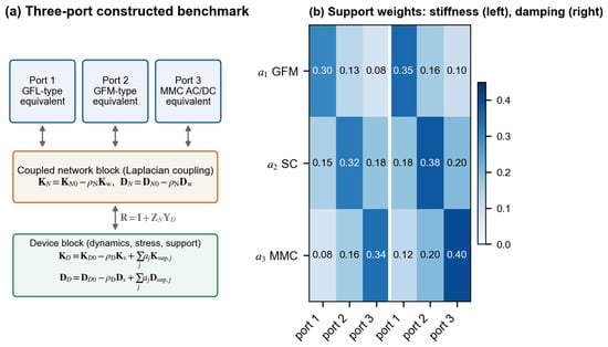
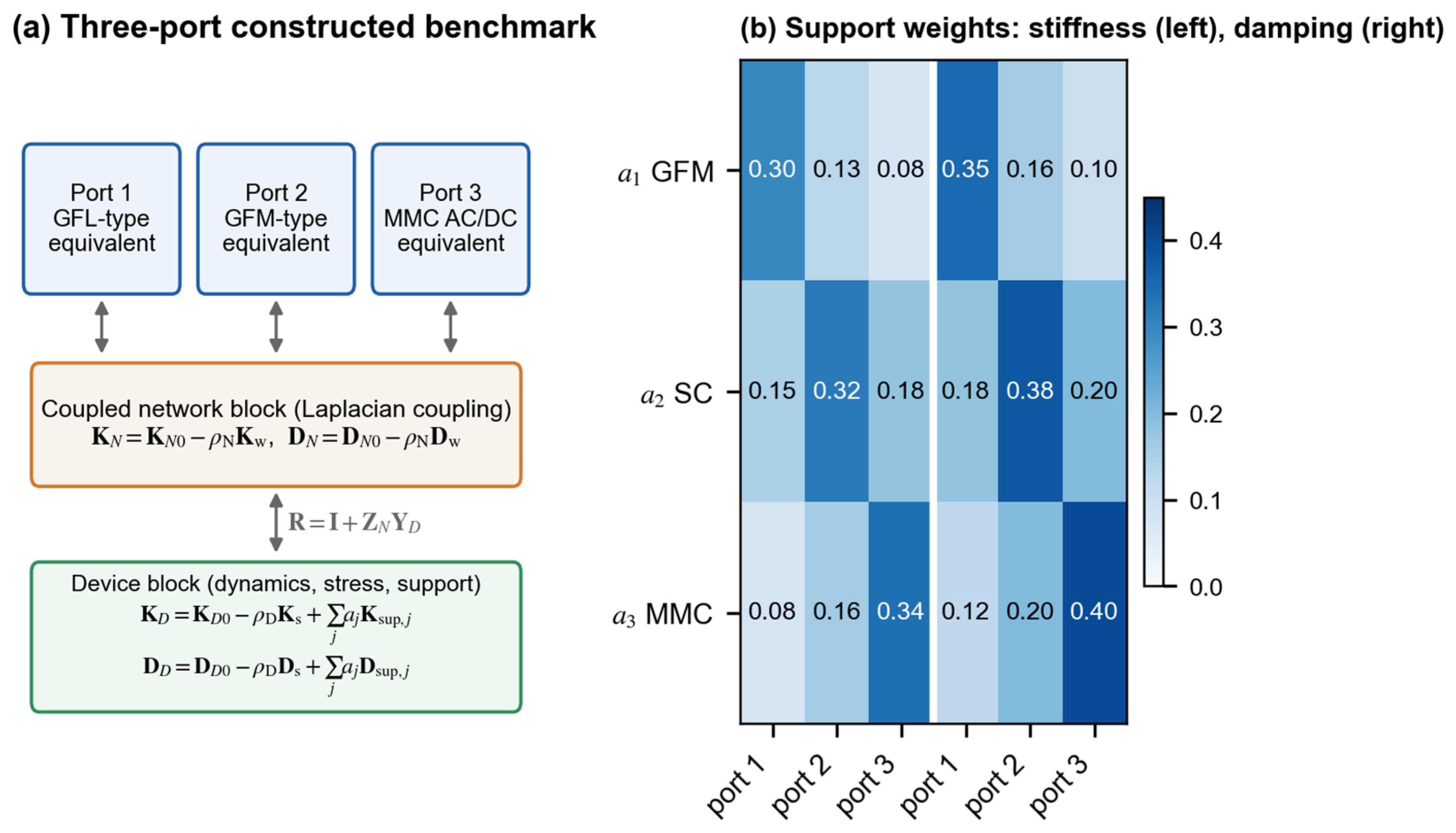
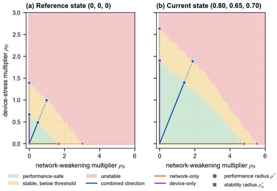
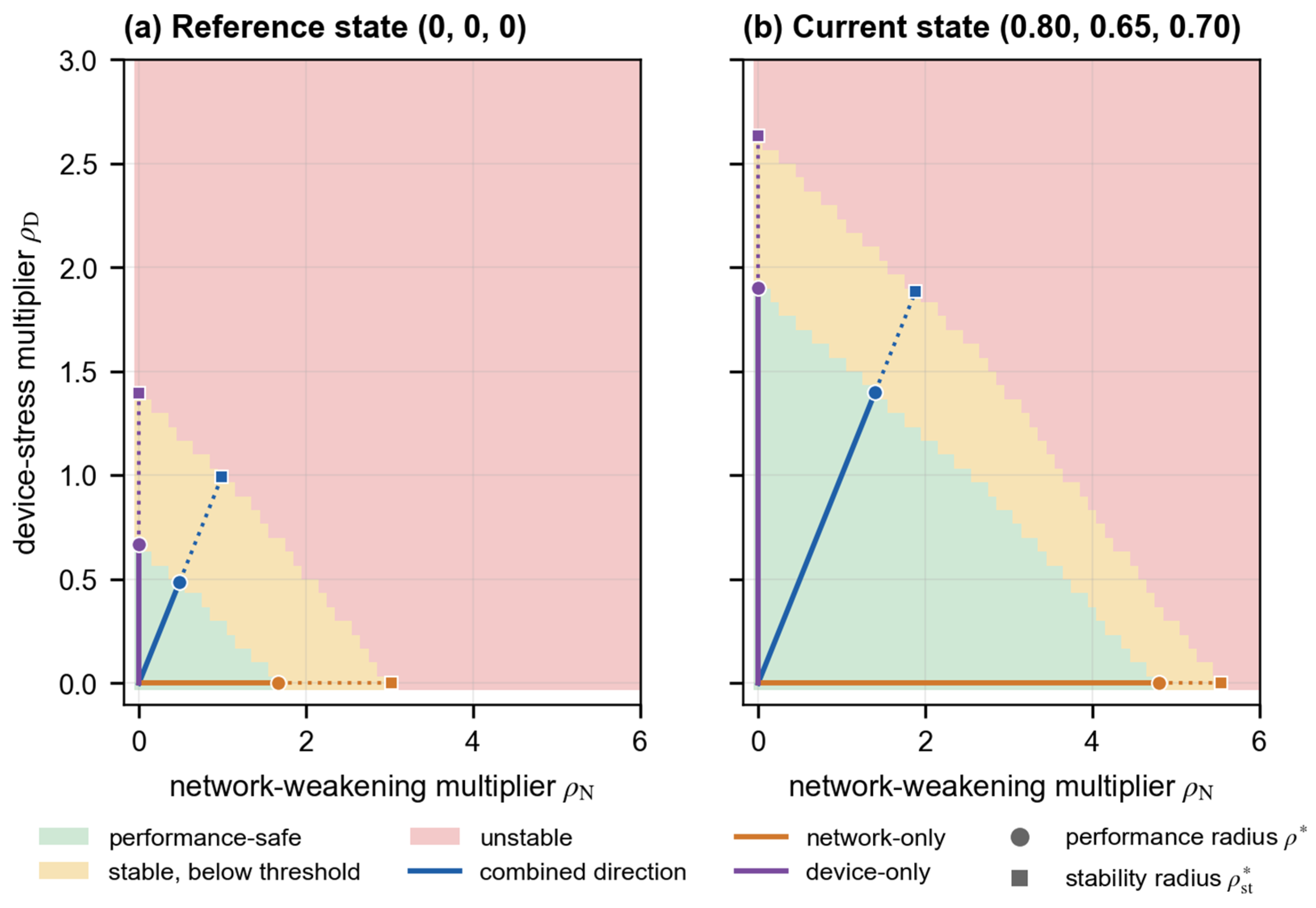
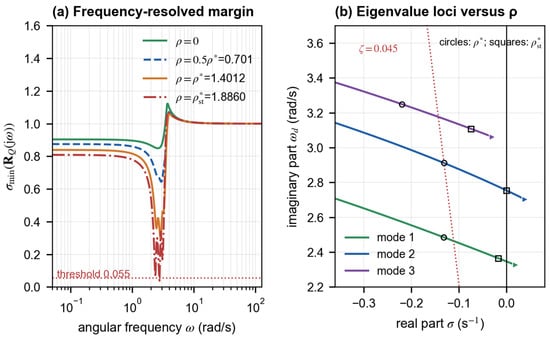
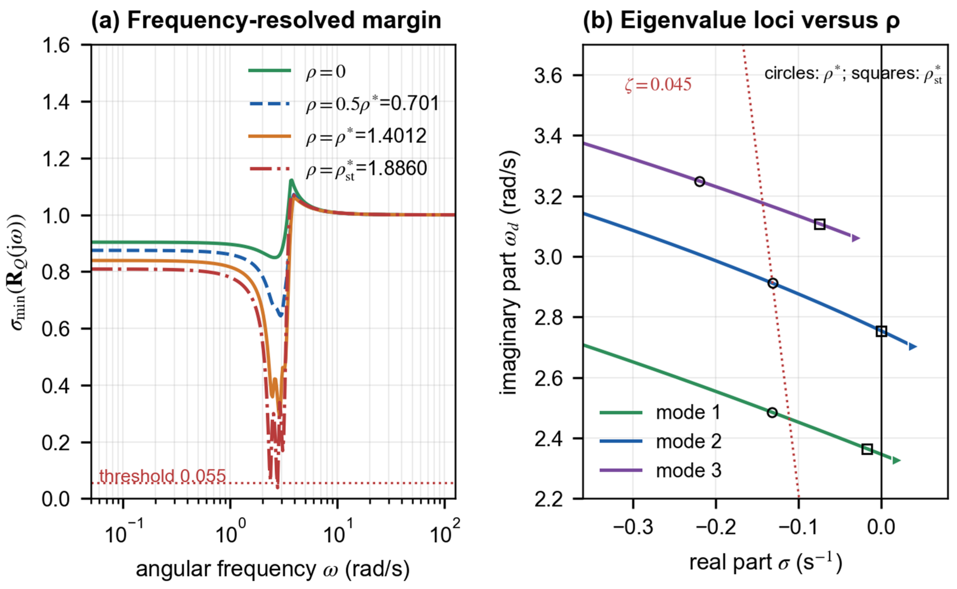
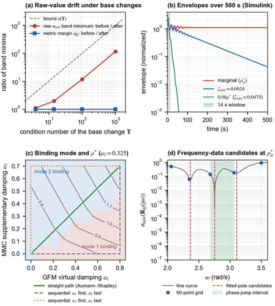
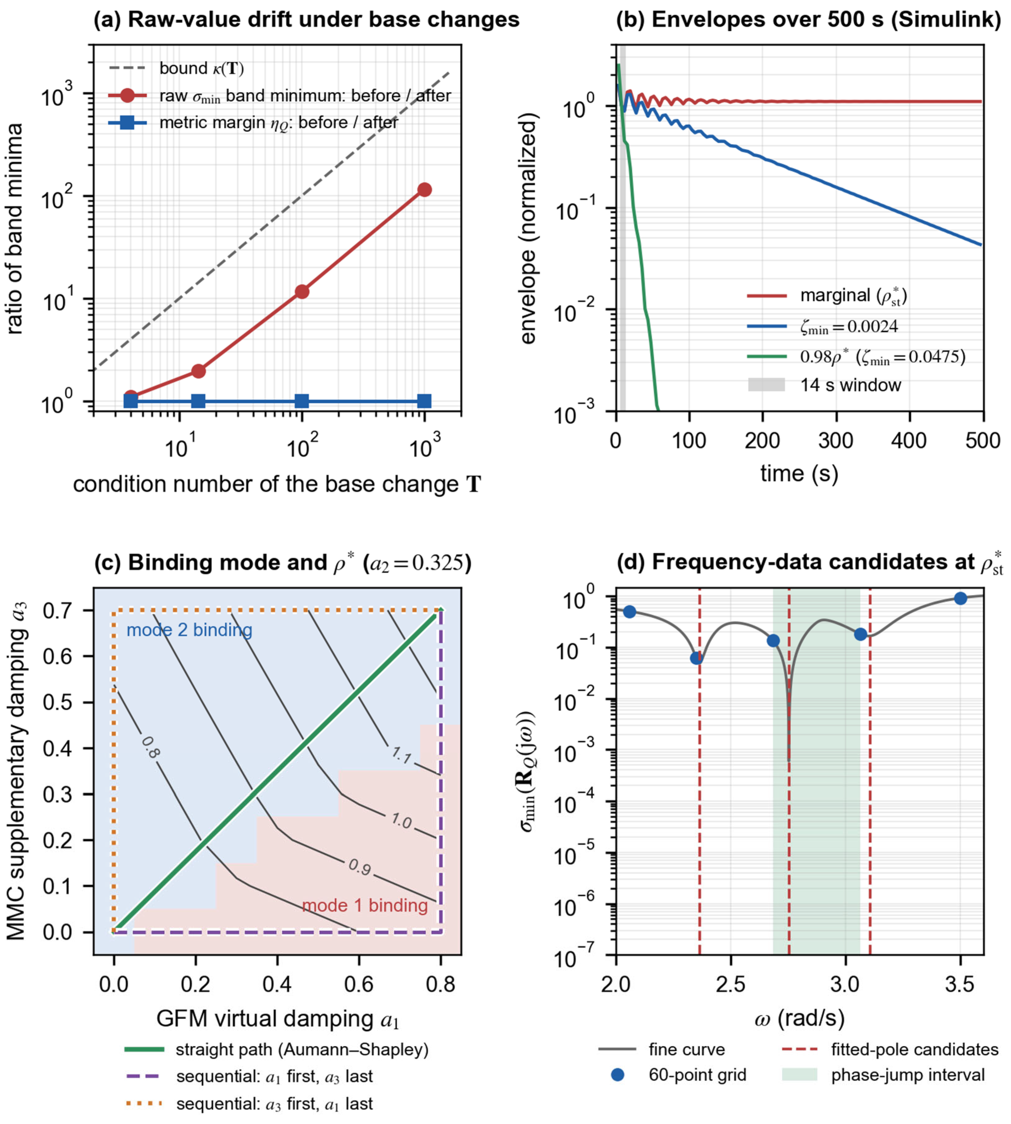
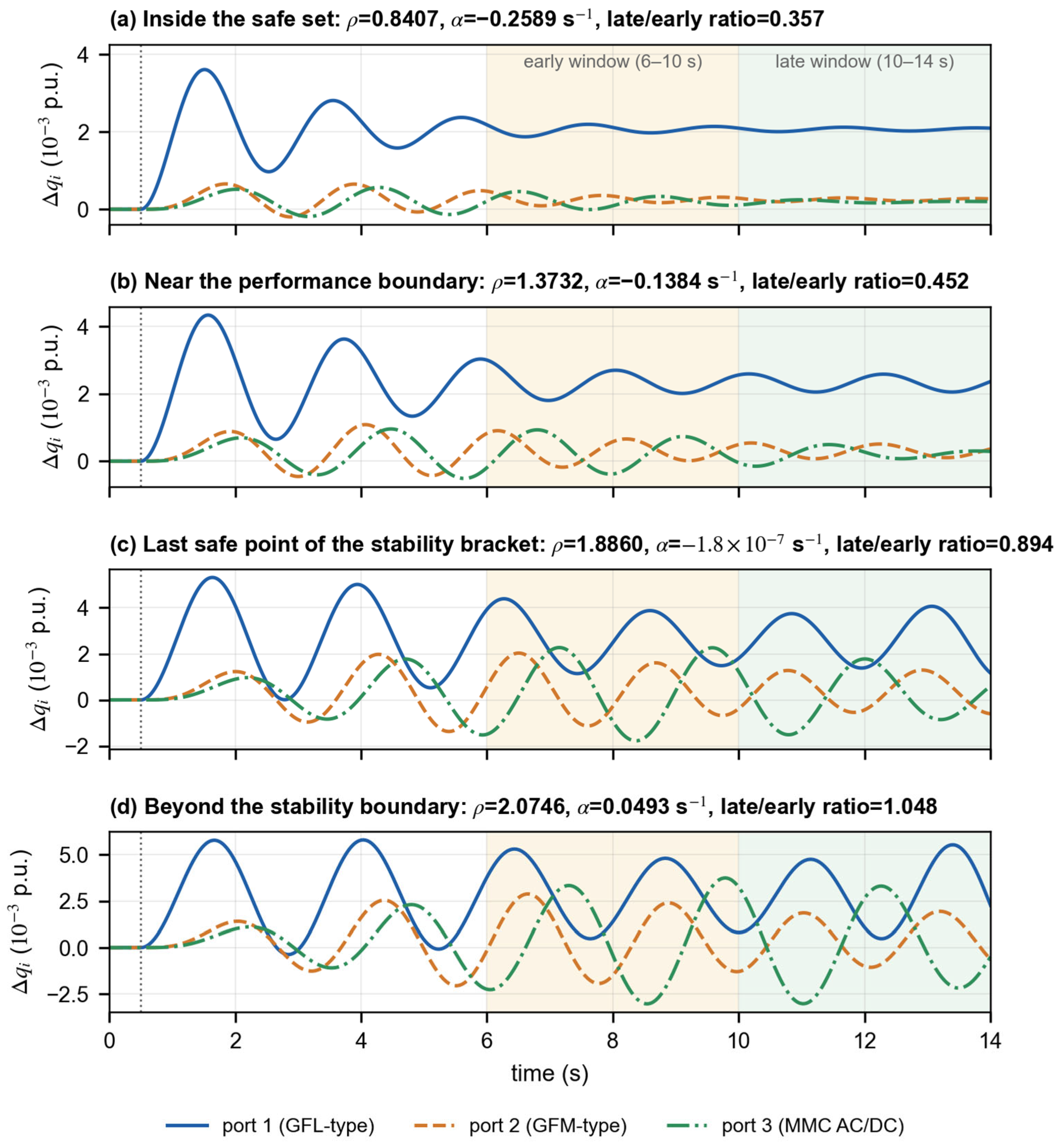
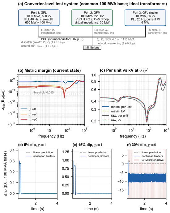
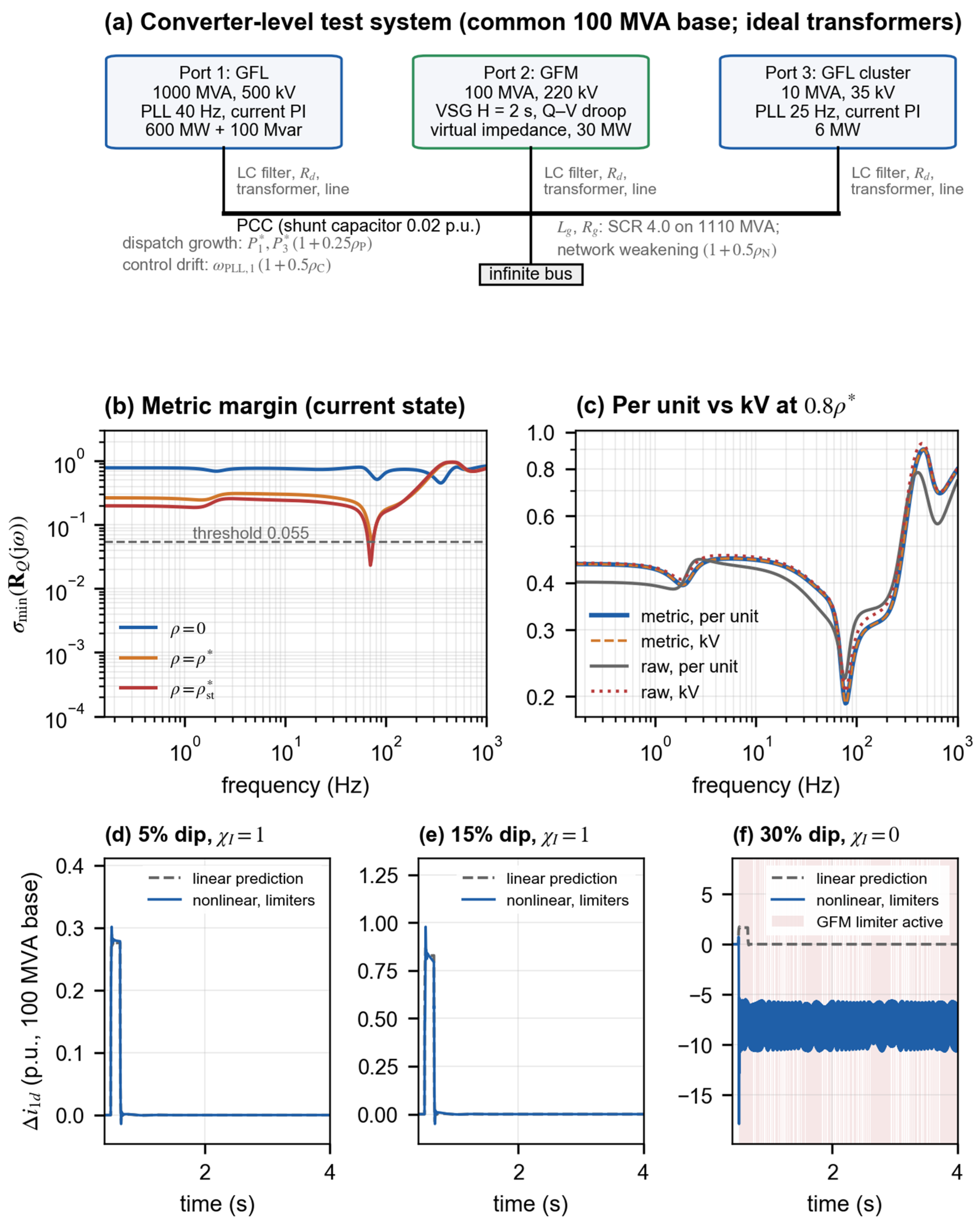

Disclaimer/Publisher’s Note: The statements, opinions and data contained in all publications are solely those of the individual author(s) and contributor(s) and not of MDPI and/or the editor(s). MDPI and/or the editor(s) disclaim responsibility for any injury to people or property resulting from any ideas, methods, instructions or products referred to in the content. |
© 2026 by the authors. Licensee MDPI, Basel, Switzerland. This article is an open access article distributed under the terms and conditions of the Creative Commons Attribution (CC BY) license.