


Abstract
Video class-incremental learning retains old knowledge while learning new actions under limited replay memory. Temporal compression stores more videos but may lose temporal details and introduce discrepancies between compressed and original videos. We propose Video Neural Memory with Bias Mitigation, combining a Spatio-Temporal Neural Memorizer and Contrastive Bias Correction. The Spatio-Temporal Neural Memorizer preserves temporal and task-related information in compact neural video representations. Contrastive Bias Correction uses class-wise adaptation prompts and contrastive learning to reduce compression-induced feature bias. Experiments on three action recognition benchmarks show higher average incremental accuracy than the compared methods under the same replay-memory budgets, including a gain of 9.18% over the strongest baseline on Something-Something V2 with 18 steps.
1. Introduction
Action recognition is a fundamental task in video understanding and has been widely studied using different data modalities, including videos [1] and sensor data collected from mobile devices [2]. However, current action recognition models are required to be finetuned on continuous video task sequences in practical scenarios, leading to a sharp decrease in the performance of previous classes, a phenomenon known as the catastrophic forgetting problem [3].
Video class-incremental learning methods explore strategies to mitigate the catastrophic forgetting problem when training an action recognition model on a sequence of independent classes. Recent video class-incremental learning methods demonstrate that storing a portion of old class videos as memory is effective in overcoming the catastrophic forgetting problem. TCD [4] stores original video frames from old tasks for memory replay to mitigate catastrophic forgetting. HCE [5] proposes a correlation refinement mechanism that uses old task memory and current task data to reduce the impact of the imbalance between old and current classes. Nevertheless, a video consists of multiple frames, which requires a large memory budget. To reduce the memory cost of videos, vCLIMB [6], VCIL-CT [7], and STSA-DFS [8] downsample the original videos along the temporal dimension. SMILE [9] stores a single frame for each original video and repeats it as a video. FrameMaker [10] constructs a condensed frame for each video to further reduce the memory cost, as shown in Figure 1a. However, these methods sacrifice the temporal details during compression, resulting in temporal misalignment during video class-incremental learning. In addition, the domain bias between the condensed frames and the original videos increases as the feature space of the incremental model changes, resulting in confusion between old and current tasks in the feature space of the current task.
Figure 1.
The comparison between VNMBM and FrameMaker (a) FrameMaker [10]. (b) VNMBM.
To address the aforementioned problems, we present a novel method, Video Neural Memory with Bias Mitigation (VNMBM), to maintain the temporal details of compressed videos in memory via a Spatio-Temporal Neural Memorizer (STNM) and correct domain bias through Contrastive Bias Correction (CBC), as shown in Figure 1b. Specifically, the STNM encodes spatio-temporal features by combining a spatial prototype with temporal indexes and decodes these features into compressed videos. As the original old task videos are inaccessible in the following tasks, we estimate their features via the knowledge distillation loss between the original video features and spatio-temporal features, allowing approximate original old class video features to be accessible in the following tasks. Additionally, we adopt a pixel reconstruction loss to capture the spatial details of the original videos. Therefore, the spatio-temporal details are maintained in the STNM, and the approximate original old class video features and compressed old class videos can be obtained from the old class STNM in the current task.
Moreover, we propose CBC to correct the current task model, which narrows the distance between compressed videos and original videos in the feature space of the current task to mitigate the domain bias and widens the distance between old and current task videos in the feature space of the current task to enhance the classification. Due to the lack of original old task videos in the current task, CBC first computes the approximate original old task video features via the STNM to represent the original old task video. As the original old task video features are computed in the old task feature space, we design learnable class-wise adaptation prompts to ensure the adaptation of approximate original old task video features to the current task feature space. Subsequently, CBC contrastively aligns and discriminates the video features in the current task feature space through a debiased contrastive loss. Moreover, the classification loss is designed to further correct the classifier. Therefore, domain bias between the compressed and original videos can be mitigated via CBC, improving the classification of old and current tasks.
The contributions of this paper can be summarized as follows:
- We introduce a memory-efficient STNM for video class-incremental learning, which can store compressed videos and approximate video features using a compact neural representation.
- We propose CBC to align the original and compressed video features and discriminate between the video features of old and current tasks in the feature space of the current task, thus mitigating the domain bias of the current task model.
- The proposed method outperforms existing methods under the same memory budget on three public benchmark datasets: UCF101, HMDB51 and Something-Something V2.
The remainder of this paper is organized as follows: We first review the related works in Section 2. Subsequently, we introduce the details of our proposed VNMBM in Section 3, following which we present the experiments and the analysis of the experimental results in Section 4. Finally, we provide a conclusion for our method in Section 5.
2. Related Work
This section reviews the literature related to our work from three aspects. We first introduce neural representations for videos as the basis for compact video memory representation, then review class-incremental learning methods for mitigating catastrophic forgetting, and finally discuss video class-incremental learning methods related to memory replay and video compression.
2.1. Neural Representations for Videos
The task of neural representation has gained increasing attention, aiming to train neural networks to regress the mapping between coordinate-like input and a given image or video. It has been widely applied in shape regression [11,12], image deblurring [13,14] and video compression. For video compression, some methods still rely on coordinates. MANIVR [15] proposes a phase-shift generation network to guide the frame-generation process. NIRVANA [16] divides videos into groups of frames and trains separate neural networks to perform a patch-wise prediction. Instead of taking coordinate-like inputs, NeRV [17] takes the frame index as the input to train the neural network representing videos. E-NeRV [18] improves NeRV by incorporating a disentangled spatio-temporal context. EC-NeRV [19] proposes a novel convolutional architecture that models the entropy of the weights and adopts quantization-aware training. Meanwhile, hybrid methods can represent videos via embeddings and decoders. HNeRV [20] uses content-adaptive embeddings as the input of the decoder, while DNeRV [21] proposes a collaborative content unit to merge the content embedding with the difference embedding. NeRV-Boost [22] introduces a temporal-aware affine transform module to improve representation capabilities and integrates a consistent entropy minimization technique to ensure the consistency between training and inference. Nevertheless, most existing neural video representation methods primarily focus on reconstructing the visual content of videos and are optimized mainly with reconstruction-oriented supervision. While this design is suitable for video representation and reconstruction, it does not specifically preserve the task-related feature representations required for video class-incremental learning. When neural representations are used as replay memory, the reconstructed old-task videos may therefore exhibit feature discrepancies from the original videos, introducing domain bias during incremental learning. In contrast, our STNM retains pixel-level reconstruction supervision while further introducing feature-level knowledge distillation and spatial prototypes to preserve the feature information of the original videos, thereby reducing the discrepancy between reconstructed and original video representations.
2.2. Class-Incremental Learning
Many class-incremental learning methods have been proposed to overcome the catastrophic forgetting problem. Existing methods mainly fall into three categories: regularization-based methods, memory-based methods and distillation-based methods.
- Regularization-Based Methods. These methods estimate the importance of model parameters and penalize the changes in the parameters associated with old tasks. EWC [23] applies a penalty based on the Fisher information matrix. PI [24] designs a synaptic framework to estimate importance weights. MAS [25] learns the importance of parameters in an unsupervised manner via the sensitivity of the output function. R-walk [26] improves EWC using a moving average and combines it with a modified PI, which uses the approximate Kullback–Leibler (KL) divergence to compute sensitivity. spWC [27] measures the discriminative contributions of old tasks via self-paced regularization.
- Memory-Based Methods. Memory-based methods focus on building the memory of old classes for memory replay. iCaRL [28] uses a herding strategy to construct memory. Mnemonics [29] parameterizes the memory using image-size parameters and then optimizes them and the model using bilevel optimization. MRDC [30] examines the trade-off between memory quality and quantity using JPEG [31] for data compression. CIM [32] proposes an adaptive mask generation model to construct 0-1 masks for discriminative pixels and downsample non-discriminative pixels. SRP [33] maintains feature distribution through class-feature sketching and projects examples into a lower-dimensional space via replay buffer projection.
- Distillation-Based Methods. These methods use knowledge distillation to transfer knowledge from the old model to the current model. LwF [34] first applies knowledge distillation in class-incremental learning by modifying the cross-entropy loss to align the outputs of the old model with those of the current model. Based on LwF, iCaRL [28] designs a nearest-mean-of-exemplars classifier for classification. LwM [35] utilizes an attention map for the attention distillation loss between the old model and the current model. To reduce feature and embedding drift, UCIR [36] proposes a less-forget constraint on features to preserve the previously learned knowledge. PODNet [37] further investigates feature constraints and introduces a pooled outputs distillation loss applied to both the embeddings and the outputs of intermediate layers. AFC [38] estimates the importance of each feature map for feature distillation. DKT [39] proposes a cluster-separation loss to encourage feature discrimination between old and new tasks. GR [40] proposes a distribution-aware knowledge distillation loss to alleviate the imbalanced catastrophic forgetting problem. Additionally, HFC [41] introduces a gradient-balanced relation distillation loss alongside a gradient-balanced forgetting compensation loss to tackle the heterogeneous forgetting speeds of different old classes.
2.3. Video Class-Incremental Learning
Although many class-incremental learning methods have been proposed in the image domain, video class-incremental learning methods have been rarely researched. TCD [4] uses a herding strategy to sample original videos for memory and proposes time-channel importance masks to facilitate time-channel distillation. HCE [5] proposes a hierarchical aggregation strategy and a correlation refinement mechanism for the alignment of spatio-temporal features. On the other hand, to compress the videos in memory, vCLIMB [6] downsamples the original videos in the temporal dimension and proposes a temporal consistency loss for regularization. VCIL-CT [7] employs temporal downsampling to store more exemplar videos under a fixed memory budget and restores the input sequence length through frame duplication during memory replay. STSA-DFS [8] introduces a difference-based frame selector that leverages global-local temporal differences and inter-task representation drift to adaptively preserve discriminative frames in the memory buffer. SMILE [9] stores a single frame for each video in memory and repeats a single frame to form a video for incremental training. FrameMaker [10] generates a condensed frame with an instance-specific prompt for each video to reduce memory costs. Although these compression-based methods have advanced video class-incremental learning, they do so at the cost of temporal details. In addition, a domain bias exists between the condensed frames and the original videos. In contrast to these methods, our VNMBM compactly compresses the videos and video features into neural representations and mitigates domain bias via a debiased contrastive loss.
3. Method
This section presents the proposed VNMBM. We first formulate the video class-incremental learning problem and introduce the datasets and task settings, followed by an overview of the proposed framework. We then describe the STNM for compact video memory representation and the CBC for bias correction, and finally present the overall training pipeline.
3.1. Problem Formulation
Video class-incremental learning methods aim to train an action recognition model , where x is the input video, f is the feature extractor and h is the final classification layer. The model is trained over a sequence of tasks , where contains the videos whose labels belong to the pre-defined label set , and . To prevent the catastrophic forgetting problem, memory-based methods construct a memory buffer to store N representative videos for each class after the incremental training step k. During the incremental training step k, the model will be trained on , where , and evaluated on all seen tasks without task boundaries.
3.2. Datasets
We evaluated our VNMBM on three standard action recognition datasets: UCF101 [42], HMDB51 [43] and Something-Something V2 [44]. The UCF101 dataset contains 13.3K videos covering 101 classes. The HMDB51 dataset contains 6.8K videos covering 51 classes. The Something-Something V2 dataset is a large-scale motion-sensitive dataset created by crowdsourcing over 174 classes, which contains 169K videos for training and 25K videos for testing.
We follow the video class-incremental settings of TCD. For UCF101, we train the initial model on 51 classes and divide the remaining 50 classes into 5, 10, and 25 incremental tasks, corresponding to 10 × 5 steps, 5 × 10 steps, and 2 × 25 steps, respectively. For HMDB51, the model is trained on 26 classes in the initial step, and the remaining 25 classes are divided into 5 and 25 incremental tasks, corresponding to 5 × 5 steps and 1 × 25 steps, respectively. For Something-Something V2, we first train the model on 84 classes, and the remaining 90 classes are divided into 9 and 18 incremental tasks, corresponding to 10 × 9 steps and 5 × 18 steps, respectively.
3.3. Overview
In this paper, we propose Video Neural Memory with Bias Mitigation (VNMBM), a novel video class-incremental learning method comprising two core components: a Spatio-Temporal Neural Memorizer (STNM) that preserves temporal details of compressed videos in memory during memory construction, and a Contrastive Bias Correction (CBC) that mitigates domain bias after memory construction. Specifically, at incremental training step k, we first train an action recognition model following TCD [4]. Then, we adopt a herding strategy to sample N original videos from each class of the current task. Instead of storing these original videos directly in memory, we train the proposed STNM for each class of the current task, which generates the compressed videos via the corresponding spatial prototypes of the original frames and the temporal indices. During the training of STNM, the knowledge distillation loss is used to align the original current task frame features and spatio-temporal features. After training the STNMs of the current task, we store the spatial prototype, the number of frames, and the STNM for each class of the current task. If , we retrain via CBC subsequent to the memory construction process. CBC first computes the spatio-temporal features as approximate original old task video features from the old task STNMs and introduces learnable class-wise adaptation prompts to adapt the approximate original old task video features to the current task feature space. Then, CBC uses a debiased contrastive loss to align and discriminate the video features in the current task feature space, and a classification loss to further correct the classifier. Thus, VNMBM achieves compact storage of compressed videos and their approximate video features through the STNM, while effectively mitigating domain bias via the CBC.
3.4. Spatio-Temporal Neural Memorizer
Existing video class-incremental methods [4,5,6,7,8,9,10] retain frame-like representations for memory replay. In contrast to existing methods, we propose the Spatio-Temporal Neural Memorizer (STNM) to construct the neural representations of the video memory buffer for more efficient memory replay. Given the temporal index and corresponding spatial prototype of the original frame, the compressed frame and approximate frame features can be constructed using the STNM, as shown in Figure 2.
Figure 2.
Illustration of STNM.
After the incremental training step k of TCD [4], we use a herding strategy [28] to select N videos from each class to construct a memory buffer and sample B frames with a uniform time interval for each video. For class , the original frames of the memory buffer are defined as , where is the j-th video in the memory buffer of class , is the q-th frame of video and .
For frame , we first compute the temporal index and normalize t between . Then, we use Positional Encoding (PE) [45] to obtain temporal embedding :
where b and l are the hyperparameters. After computing the temporal embedding, we construct the spatial prototype from the trained feature extractor . For a video of class , the feature extractor produces , where B denotes the number of sampled temporal positions and denotes the feature dimension. Each row of therefore represents the feature at one sampled temporal position. The spatial prototype of class is obtained by averaging the features of all training videos in this class:
where is the number of videos in class . The spatio-temporal encoder is designed to combine temporal embedding with the spatial prototype, and the spatio-temporal feature is computed as follows:
where is a linear layer, and denotes the q-th row of the spatial prototype , corresponding to the q-th sampled temporal position. When , 1D max pooling downsamples from to dimensions before its element-wise multiplication with the -dimensional encoder output. The resulting -dimensional spatio-temporal feature is then fed into the decoder.
Subsequently, a linear layer is used to compute the linear projection of the spatio-temporal feature , which is stacked with four NeRV blocks [17] as the decoder to decode the spatio-temporal feature into a compressed frame . These NeRV blocks utilize convolution layers, PixelShuffle layers [46] and swish activation layers [47] for upsampling. To adjust the channel dimension to 3, we add a convolution layer at the end of the final NeRV block. Therefore, the compressed frame of the compressed memory buffer is constructed from the normalized temporal index t, spatial prototype and STNM of class :
To reduce the domain bias between the compressed frame and the original frame , we first use the combination of the L1 loss and the SSIM loss [17] as the pixel reconstruction loss to supervise the STNM at the pixel-level:
where is set to 0.7, represents the L1 norm, represents the structural similarity index measure and . In addition, we use the feature extractor to compute the original current task frame feature and design the knowledge distillation loss to make the expression of the original current task frame feature and spatio-temporal feature similar:
where is the Frobenius norm. When , 1D max unpooling is applied to the -dimensional spatio-temporal feature before computing . Using the indices obtained from prototype pooling, the unpooling produces a -dimensional feature that matches the dimension of . Unpooling is used for feature matching and does not change the -dimensional input to the decoder. When , neither pooling nor unpooling is required. is obtained by normalizing the time-channel importance mask [4] computed from the final output of the feature extractor . After the incremental training of task k and before memory construction, the unnormalized importance at temporal position q and channel c is estimated as
where contains the original current task videos and the compressed replay videos from previous tasks. denotes the feature at the q-th sampled temporal position and the c-th channel in the final output of for video x. denotes the classification loss of the recognition model for video x and its label y. For the first task, . The importance mask is computed from the gradients of the classification loss with respect to the recognition features and remains fixed during subsequent STNM training.
Hence, the final objective function of the STNM is given by the following equation:
where is set to 0.001 for all tasks. After training the STNM in step k, we store the spatial prototype p, the number of frames T and the STNM G of each class in and use them to construct in the following tasks.
For different memory budgets, we change the STNM architecture to obtain STNM models with different sizes. The STNM architecture is shown in Table 1. As shown in Table 1, we design NeRV blocks with different upscale factors to gradually upsample the hidden dimensions h and w from to and adjust and to obtain STNM models with different sizes. In addition, the setting of is related to the dimension of the original video features, as we want to store the approximate original old task video features in the STNM, and the setting of is decided by and the memory budget. We use 8-bit quantization [17] for the STNM parameters. The 8-bit quantization of the parameter tensor can be represented as:
where and denote the n-th original parameter in the parameter tensor and its dequantized approximation, respectively. and denote the minimum and maximum values of , respectively. maps a value to the nearest integer. The scale and are stored as part of the memory budget for dequantization.
Table 1.
The STNM architecture for videos with a resolution of pixels. denotes the spatial prototype dimension, while and are adjusted to obtain STNM models with different sizes. FC represents a linear layer with a learnable bias, and Conv represents a convolutional layer with the learnable bias. Block represents the NeRV block. Here, denotes the largest integer not greater than x, and the max operation ensures a minimum of 96 output channels in Blocks 2 to 4.
The memory budget of each class consists of an STNM, a spatial prototype, a frame count, and the quantization parameters (scale and ). All storage sizes below are expressed in bytes:
Under 8-bit quantization, each quantized STNM weight or bias is stored using one byte. Based on the architecture in Table 1, the storage required for a STNM is
The spatial prototype contains elements, where denotes the prototype feature dimension. Since each element is stored in FP32 format, its storage requirement is
The frame count T is stored as a single 32-bit integer, requiring
The quantization parameters, scale and , are stored in FP32 format, requiring four bytes per scalar. Based on the architecture in Table 1, their total storage requirement is
The layer-wise storage breakdown of STNM is summarized in Table 2. The layer storage is obtained by counting the weights and biases of each learnable layer in Table 1. Under 8-bit quantization, each quantized parameter occupies one byte. The corresponding quantization storage includes the FP32 scale and values required for dequantization. Layers without learnable parameters are excluded from the storage calculation.
Table 2.
Layer-wise storage of a STNM. Layer storage includes 8-bit weights and biases, while quantization storage includes the FP32 scale and . All sizes are reported in bytes.
By combining the above four components, the per-class memory budget is obtained as
3.5. Contrastive Bias Correction
Although STNM mitigates domain bias between the compressed and original videos, the trained model of the current task is trained on the combination of the original current task videos and the compressed old task videos, resulting in the accumulation of domain bias. Therefore, we propose Contrastive Bias Correction (CBC) to separate the distribution of current task videos from old task videos while bringing the distribution of compressed videos and original videos closer together, as shown in Figure 3.
Figure 3.
Illustration of CBC. Lock/unlock icons indicate frozen/trainable weights.
Specifically, after the step k training of the STNM, given a compressed video and a corresponding original video for the j-th video in the memory buffer of class , we first compute the original current task video feature and the compressed current task video feature via the feature extractor .
Meanwhile, we randomly select a video index of class , where . The temporal index set s of video index is defined as , and we compute the approximate original old task video feature using the following formula:
where is the spatial prototype of class . Then, we feed into and obtain the compressed video , which is used to compute the compressed old task video feature .
The approximate original old task video feature is close to the original old task video feature in the old task feature space. To adapt to the feature space of the current task k, we design a learnable class-wise adaptation prompt for class . Thus, can be updated as follows:
Domain bias between the compressed and original videos leads to confusion between old and current tasks. To reduce domain bias, the compressed and original videos should be mapped to nearby features in the feature space of the current task k, and the old and current task videos should be mapped to distant features in the feature space of the current task k. Therefore, CBC computes the distance between the compressed and original videos in the feature space of the current task k as follows:
where is the cosine similarity, is the cosine distance, L is the number of classes in the current task k and N is the number of compressed videos stored in the STNM.
Then, CBC computes the similarity between the old and current task videos in the feature space of the current task k as follows:
Based on the distance between the compressed and original videos and the similarity between the old and current task videos, CBC introduces a debiased contrastive loss to pull the compressed and original videos together and push away old and current tasks in the feature space of the current task k, which is defined as follows:
In addition, the video features are fed into the classification layer , and we compute Neighborhood Component Analysis (NCA) loss [48] as classification loss to optimize the feature extractor and classification layer , which is computed from the Local Similarity Classifier (LSC) following PODNet [37].
Therefore, the final objective function of the CBC is given as follows:
where is set to 1 for all tasks.
3.6. Overall Training Pipeline
To provide a concise overview of the proposed VNMBM, Algorithm 1 details the complete training pipeline across three distinct stages for each incremental task. In Stage 1 (Incremental Training), our method reconstructs compressed old task video frames from the frozen STNMs using the stored spatial prototypes, the number of frames, and quantization parameters. It then trains the action recognition model using a combination of the original current task video frames and the reconstructed compressed old task video frames. During Stage 2 (Memory Construction), our method trains the new STNMs for the current classes and stores them alongside their corresponding spatial prototypes, the number of frames, and quantization parameters. Finally, in Stage 3 (Contrastive Bias Correction), our method initializes trainable class-wise adaptation prompts to retrain the action recognition model while keeping all STNMs strictly frozen, ultimately removing the prompts.
| Algorithm 1 Overall Training Pipeline of VNMBM |
Input: Sequential task raw data , where Output: The action recognition model
|
4. Experiments
This section evaluates the proposed VNMBM. We first introduce the evaluation metrics and implementation details, followed by comparisons with existing methods. We then conduct ablation studies and further analyses to evaluate the contributions of the proposed components and investigate their performance under different settings.
4.1. Evaluation Metrics
Following previous video class-incremental methods [4,5,6,7,8,9,10], we apply the average incremental accuracy using CNN and NME to evaluate the performance of video class-incremental learning, which can be defined as follows:
where CNN and NME are two inference methods. CNN classifies test videos using the trained fully connected layer. For NME evaluation [28], after the completion of CBC, we use the updated feature extractor to compute the class-mean features from the reconstructed videos in the memory buffer. Test videos are then classified by comparing their feature embeddings with these class means. Therefore, both the class means and test video features are obtained using the recognition model after CBC when . and are the average accuracies using CNN and NME in all the seen categories for the incremental training step k.
Peak signal-to-noise ratio (PSNR) is adopted to evaluate the quality of compressed frames, which is the ratio of the maximum value of the pixel to the mean squared error between the original and compressed frames. The higher the PSNR, the better the quality of the compressed frames. PSNR can be denoted as follows:
where is the maximum possible pixel value of the image, and is the mean squared error between the original and compressed frames.
4.2. Implementation Details
We implement our method based on TCD [4], following the training hyperparameters and data pre-processing steps of TCD. The dimensions of each frame are , where and . During the incremental training of TCD, the compressed old task videos are constructed using old task STNMs for memory replay. After the incremental training of TCD, we train the STNMs to construct the neural representations of the current task video memory buffer and use the CBC to retrain the TCD. For the STNM, b and l of PE are set to 1.25 and 40, respectively. We stack four NeRV blocks with upscale factors of 4, 2, 2, 2, and the hidden dimensions h and w are both set to 7. According to the upscale factors of the NeRV blocks, these blocks gradually upsample the hidden dimensions h and w from to . We adjust the model size of the STNM based on Equation (11). The STNM configurations under different datasets and backbones are summarized in Table 3. The spatial prototype dimension is determined by the dimension of the backbone output features used to construct the spatial prototype, which is 512 for ResNet-34 TSM [1,49], 2048 for ResNet-50 TSM [1,49], and 1024 for CLIP ViT-L/14 [50]. The internal channel dimensions and of STNM are adjusted according to the memory budget. Specifically, are set to , , , and for the 1.2 Mb, 2.4 Mb, 6.0 Mb, and 24.0 Mb STNMs, respectively. When , 1D max pooling is applied to downsample the spatial prototype from to dimensions before its element-wise multiplication with the encoder output. The corresponding 1D max unpooling operation restores the spatio-temporal feature from to dimensions for feature matching. When , these pooling and unpooling operations are not required. The detailed per-class memory budget under each experimental setting is reported in Table 4, including the quantized STNM parameters, spatial prototype, frame count, and quantization parameters. The exact total memory is calculated according to Equation (15). The quantization overhead introduced by storing the FP32 scale and parameters is calculated as the percentage of the total per-class memory occupied by these parameters and is reported in Table 4. Mb represents Mbytes.
Table 3.
STNM configurations under different datasets and backbones. Sth-Sth V2 denotes the Something-Something V2 dataset.
Table 4.
Memory budget and quantization overhead of VNMBM under different experimental settings. Sth-Sth V2 denotes the Something-Something V2 dataset.
We use the Adam optimizer to train the STNM, with a batch size of 32. The Adam optimizer uses , , , and a weight decay of 0. The initial learning rate is set to 0.004 for the 6.0 Mb, 2.4 Mb, and 24.0 Mb STNMs and 0.006 for the 1.2 Mb STNM. The STNM is trained for 300 epochs. For STNM training, we adopt a cosine annealing learning rate schedule with a warmup period of 60 epochs. We use a herding strategy [4] to select , , and videos per class for training the 6.0 Mb STNM on UCF101, the 24.0 Mb STNM on Something-Something V2, and the 6.0 Mb STNM on HMDB51, respectively. We sample frames with a uniform time interval for each video. After training the STNM, we use 8-bit quantization [17] for the STNM. After the training of the current task STNMs, we use CBC to train the current task TCD for 40 epochs. The batch size is set to 8 for UCF101 and 16 for HMDB51 and Something-Something V2. The SGD optimizer is deployed for CBC. The initial learning rates of the TCD and class-wise adaptation prompts are 0.0001 and 0.001, respectively. During CBC training, both learning rates are multiplied by 0.1 at epoch 20. The weight decay of CBC is set to . For UCF101 and HMDB51, following TCD [4], we use random seeds 1000, 1993, and 2021. Since the random seed also determines the class order, these three runs correspond to three different class orders. We report the mean and standard deviation over the three runs. For Something-Something V2, following TCD [4], we use the single-seed setting with seed 1000. The complete class orders corresponding to these random seeds are provided in Appendix A Table A1, Table A2, and Table A3, respectively.
4.3. Main Results
In this section, we compare our proposed approach with the existing class-incremental learning approaches on the UCF101, HMDB51 and Something-Something V2 datasets. For the UCF101 and HMDB51 datasets, Fine-tuning, LwFMC [34], LwM [35], iCaRL [28], UCIR [36], PODNet [37], TCD [4], FrameMaker [10], and HCE [5] employ ResNet-34 TSM and ResNet-50 TSM [1,49] as their respective backbones, both initialized with ImageNet-pretrained weights [51]. In contrast, VCIL-CT [7] and STSA-DFS [8] adopt the CLIP ViT-L/14 backbone [50] for both datasets. For the TSM settings, VNMBM uses ImageNet-pretrained ResNet-34 TSM on UCF101 and ResNet-50 TSM on HMDB51. For the CLIP ViT-L/14 settings, VCIL-CT, STSA-DFS, and VNMBM use the official OpenAI CLIP ViT-L/14 pretrained weights. Following STSA-DFS [8], the feature extractor of VNMBM consists of a frozen CLIP ViT-L/14 image encoder and a trainable Spatial-Temporal Side Adaptation (STSA) module [8]. The STSA module performs temporal modeling on classification tokens and spatial modeling on patch features extracted from the CLIP image encoder, and integrates the resulting representations for action classification. Therefore, the CLIP settings of VNMBM directly use CLIP visual features without relying on TSM for feature extraction. For the Something-Something V2 dataset, UCIR, PODNet, TCD, FrameMaker and HCE use the ResNet-50 TSM as backbone, which is initialized by ImageNet pretrained weights. For a fair comparison, we evaluated our method using the same model architecture and pre-training initialization as the existing video class-incremental learning methods [4,10]. For the memory-based comparison methods, including iCaRL, UCIR, PODNet, TCD, FrameMaker, HCE, VCIL-CT, and STSA-DFS, video frames are stored as replay memory. The memory budget is set to 6.0 Mb per class for UCF101 and HMDB51 and 24.0 Mb per class for Something-Something V2. VNMBM follows the same memory budget for a fair comparison, while its replay memory is stored in the form of neural representations rather than video frames. Specifically, the memory budget of VNMBM includes the quantized STNM parameters, spatial prototypes, frame count, and quantization parameters. In Table 5, Fine-tuning, LwFMC, and LwM do not store replay exemplars, corresponding to 0 bytes of exemplar replay memory per class. For iCaRL, UCIR, PODNet, TCD, FrameMaker, HCE, VCIL-CT, and STSA-DFS, the per-class replay-memory budget corresponds to 40 RGB frames of size stored in uint8 format, requiring bytes per class, denoted as 6.0 Mb in our experiments. FrameMaker stores 40 condensed frames within this budget. These per-class budgets apply to all reported task splits and CNN/NME columns on UCF101 and HMDB51 in Table 5.
Table 5.
Comparison with existing video class-incremental learning methods on the UCF101 and HMDB51 datasets. VNMBM achieves the best performance among the compared methods under the evaluated settings. Results marked with * are taken from HCE [5], while those marked with † are taken from STSA-DFS [8]. The results of VNMBM are presented as means ± standard deviations over three class orders generated using seeds 1000, 1993, and 2021, as detailed in Appendix A.
Table 5 reports the overall results on UCF101 and HMDB51. Under the evaluated memory budgets and backbone settings, VNMBM achieves the best performance among the compared methods across all configurations. Under the TSM setting, VNMBM surpasses HCE by up to 1.67%, 2.77%, and 2.76% in CNN accuracy on the three UCF101 settings and by up to 4.25% and 7.16% on the two HMDB51 settings, respectively. Under the CLIP ViT setting, VNMBM also outperforms the recent STSA-DFS method across all evaluated configurations. These results show that VNMBM provides favorable recognition performance under the evaluated video class-incremental learning settings and memory budgets.
Table 6 reports the overall results obtained on the large-scale motion-sensitive Something-Something V2 dataset. Our VNMBM outperforms HCE by up to 6.41% and 9.18% on the Something-Something V2 dataset with 9 steps and 18 steps, respectively. These results indicate that our method effectively maintains temporal information in the STNM while mitigating the domain bias problem caused by compression, thereby offering both high memory efficiency and superior performance.
Table 6.
Comparison with existing video class-incremental learning methods on the Something-Something V2 dataset. Results marked with * are taken from HCE [5].
4.4. Ablation Study
The figures in this section were prepared using Matplotlib 3.5.3 (Python 3.7.16) and Microsoft PowerPoint 2021. No additional calibration was applied to the experimental measurements.
- Effect of each component. To investigate the contributions of the individual components in STNM and CBC, we conduct ablation experiments by progressively introducing different components, and the results are summarized in Table 7. The Baseline represents TCD storing 40 frames from five videos per class under a memory budget of 6.0 Mb. The Baseline accuracies are taken from the original TCD publication [4], which does not report standard deviations. The remaining ablation configurations are evaluated using three seeds (1000, 1993, and 2021), with results reported as mean ± standard deviation.Table 7. Ablation study of different components of STNM and CBC on UCF101 with 10 steps. PE denotes positional encoding used for temporal encoding.
For STNM, using only the pixel reconstruction loss achieves CNN and NME accuracies of 44.82% and 37.10%, respectively. provides pixel-level reconstruction supervision and does not specifically target perceptual or discriminative features for action recognition. After introducing positional encoding for temporal encoding, the CNN and NME accuracies increase substantially to 77.22% and 77.30%, respectively. Without temporal encoding, STNM has difficulty representing high-frequency information from the temporal input, resulting in much lower performance. Positional encoding provides a richer representation of the temporal input and improves the modeling of video content at different temporal positions. On this basis, adding the knowledge distillation loss further improves the CNN and NME accuracies to 78.16% and 78.31%, respectively. provides feature-level supervision to preserve information extracted from the original videos. Incorporating the spatial prototype further increases the accuracies to 78.94% and 78.82% by introducing class-related feature information, forming the complete STNM. Compared with the Baseline, the complete STNM improves the CNN and NME accuracies by 5.51% and 3.47%, respectively, showing higher recognition accuracy than frame-based replay under the same memory budget.
Based on the complete STNM, introducing increases the CNN and NME accuracies to 79.08% and 79.28%, respectively. Further introducing improves the accuracies to 79.69% and 79.64%. Finally, incorporating the class-wise adaptation prompt achieves 80.36% and 80.17%, respectively. These results show the progressive contributions of the components in STNM and CBC to the final recognition performance.
- Different STNM configurations. To evaluate the effect of different STNM configurations, we design the VNMBM in different sizes for each class to store 40 compressed videos per class on the UCF101 dataset with 10 steps. Then, we compute the average accuracy of each task and the mean PSNR of the compressed frames for each class to represent the per-task accuracy and per-class quality, respectively. Specifically, PSNR is calculated between each compressed frame and its corresponding original frame. The results are shown in Figure 4, which shows that the larger VNMBM can achieve better compression quality when storing the same number of videos, thereby better mitigating the catastrophic forgetting problem. Notably, we introduce the compression quality metric to explicitly explore the behavior of our neural memory paradigm. By jointly analyzing the per-task accuracy and the per-class quality in Figure 4, we observe a phenomenon of diminishing marginal returns. Specifically, the growth in per-class quality from the 2.4 Mb VNMBM to the 6.0 Mb VNMBM is higher than the growth from the 1.2 Mb VNMBM to the 2.4 Mb VNMBM. However, the corresponding increase in per-task accuracy exhibits the exact opposite trend. This phenomenon provides an additional insight: the marginal benefit of solely improving image quality diminishes for downstream classification. It reveals that under a given memory budget, relying exclusively on higher video quality is suboptimal; one must comprehensively balance both the quantity and the quality of the stored videos. This finding motivates our subsequent further exploration regarding the trade-off between video quantity and quality in the following section.Figure 4. Per-task accuracy and compressed-video quality on UCF101 with 10 steps.
- Effect of the quality of compressed videos under different memory budgets. To show the effect of the quality differences at various memory budgets, we first construct 6.0 Mb VNMBM, 2.4 Mb VNMBM and 1.2 Mb VNMBM for the 6.0 Mb, 2.4 Mb and 1.2 Mb memory budgets. Then, we store different numbers of videos in these models for various compression qualities and use the mean PSNR of the compressed frames for all the classes to measure the compression quality. The results are shown in Table 8. When the number of stored videos N is fixed, increasing the memory budget improves the reconstruction quality of the compressed videos, as indicated by the higher PSNR, and is accompanied by higher CNN and NME accuracies. For example, when , the PSNR increases from 28.36 dB to 36.62 dB as the memory budget increases from 1.2 Mb to 6.0 Mb, while the CNN and NME accuracies increase from 74.58% and 77.35% to 79.95% and 79.91%, respectively. Specifically, increasing the memory budget from 1.2 to 2.4 Mb yields a PSNR gain of 3.09 dB, accompanied by CNN and NME accuracy gains of 3.78% and 1.90%, respectively. Increasing the budget further to 6.0 Mb yields a larger PSNR gain of 5.17 dB but smaller CNN and NME accuracy gains of 1.59% and 0.66%, respectively, indicating diminishing accuracy improvements despite greater reconstruction quality gains. When the memory budget is fixed, increasing the number of stored videos reduces the memory allocated to each video and therefore decreases the reconstruction PSNR. However, the recognition performance does not necessarily decrease accordingly. For example, under the 6.0 Mb memory budget, increasing N from 20 to 80 decreases the PSNR from 36.84 dB to 36.30 dB, while the CNN and NME accuracies increase from 76.80% and 79.34% to 80.36% and 80.17%, respectively. These results show that reconstruction quality and downstream recognition performance are not monotonically correlated under a fixed memory budget. The final recognition performance reflects a trade-off between the reconstruction quality of the compressed videos and the number of stored videos. For the 1.2 Mb memory budget, achieves better recognition performance than and , suggesting that storing too many heavily compressed videos may reduce the benefit of increasing the number of replay videos. Therefore, we set for the 6.0 Mb and 2.4 Mb VNMBMs, and for the 1.2 Mb VNMBM. We also visualize the compressed frames under different memory budgets in Figure 5. For this visualization, all three VNMBMs encode videos per class. From the visualization results, it can be observed that the motion information of the compressed videos is well preserved under different memory budgets, which demonstrates that our VNMBM ensures the high quality of compressed frames.Table 8. Analysis of the effect of quality differences at various memory budgets on the UCF101 dataset with 10 steps. N is the number of compressed videos stored in the VNMBM. PSNR represents the mean PSNR of compressed frames for all UCF101 classes.Figure 5. Compressed frames under different memory budgets on UCF101 with 10 steps. The compressed results in panels (b–d) correspond to videos per class.
- Memory budget comparison. We compare VNMBM with existing approaches under different memory budgets, and the results are reported in Table 9. The HCE results are taken from [5]. Both HCE and VNMBM follow the incremental task split settings established by TCD [4]. The class orders used for VNMBM are provided in the Appendix. From these results, we observe that our method using the 2.4 Mb memory budget can achieve better performance than HCE using the 6.0 Mb memory budget. Meanwhile, the performance of our method can be further improved by using the same memory budget as existing methods. These results demonstrate the effectiveness of our method in alleviating the catastrophic forgetting problem under the limited memory budget.Table 9. Memory budget comparison on the UCF101 dataset with 10 steps. Existing methods store the frame-like memory, while our VNMBM stores the neural representations.
- Effect of class-wise adaptation prompts. To evaluate the effect of class-wise adaptation prompts in CBC, we conduct experiments with different numbers of adaptation prompts. The “None” setting retains the complete STNM and uses both the classification loss and the debiased contrastive loss in CBC, without adaptation prompts. The results in Table 10 show that CBC with a shared adaptation prompt for all old classes outperforms CBC without the adaptation prompt, which indicates that the adaptation prompt adapts the original old task video features to the current task feature space. Moreover, CBC using class-wise adaptation prompts leads to further improvements in performance. This configuration assigns a learnable class-wise adaptation prompt for each class of old tasks and adapts the original old task video features according to the distribution of each class.Table 10. Ablations for different numbers of adaptation prompts in Contrastive Bias Correction on the UCF101 dataset with 10 steps.
- Effect of CBC on mitigating the domain bias. The domain bias refers to the difference between compressed and original videos. To evaluate the domain bias, we calculate the per-class feature distances between compressed and original videos of the initial 51 classes at the incremental step 2 on the UCF101 dataset with 10 steps. Specifically, we feed the compressed and original videos of each class within the initial 51 classes into the feature extractor, obtaining compressed old task video features and original old task video features, respectively. For each compressed-original video pair, we then compute the Frobenius norm of the difference between their corresponding video features. The mean of the Frobenius-normalized results for each class is the per-class feature distance between compressed and original videos. A larger per-class feature distance indicates a more significant domain bias between compressed and original videos. The results are summarized in Figure 6. As shown in this figure, all classes exhibit non-zero feature distances, which proves that there is a difference between compressed and original videos, i.e., domain bias exists. Additionally, our CBC reduces the feature distances across all 51 classes, which demonstrates that CBC effectively mitigates domain bias.Figure 6. Comparison of feature distances before and after our CBC.
To further investigate cross-task confusion, we calculate the average softmax probability mass assigned to the opposite task group using compressed old-class videos and original current-class videos. Specifically, we apply softmax over all 56 seen classes, sum the probabilities assigned to the 5 current classes for each compressed old-class video or to the 51 old classes for each original current-class video, and then average over the corresponding samples. The same samples are evaluated before and after CBC. As shown in Table 11, the old-to-new probability mass decreases from 4.38% to 1.93%, corresponding to a relative reduction of 55.94%. Similarly, the new-to-old probability mass decreases from 11.43% to 4.86%, corresponding to a relative reduction of 57.48%. These results indicate reduced cross-task probability assignment after CBC, providing additional evidence beyond feature alignment.
Table 11.
Cross-task probability mass before and after CBC at incremental step 2 on UCF101 with 10 steps.
To further evaluate the effect of feature alignment on recognition performance, we compare the classification accuracies before and after CBC on the held-out UCF101 test set containing all 56 seen classes at incremental step 2. As shown in Table 12, the CNN and NME accuracies increase from 83.05% and 83.68% to 84.89% and 84.50%, corresponding to improvements of 1.84% and 0.82%, respectively. These results show that the reduction in feature distance after CBC is accompanied by improved classification accuracy on unseen test videos.
Table 12.
Classification accuracy before and after CBC on the held-out UCF101 test set with 56 seen classes at incremental step 2.
- Quantitative analysis of feature separability. To further evaluate the effect of CBC on class separability, we perform a quantitative analysis on the test set of the 56 seen classes at incremental step 2 on UCF101 with 10 steps. We use the feature extractors before and after CBC to extract the corresponding test features, respectively. For each stage, the mean feature of each class is independently computed as its class center. We use cosine distance as the distance metric. The average intra-class distance is calculated by first computing the average cosine distance between the samples of each class and their corresponding class center and then equally averaging the results over all 56 classes. The average inter-class distance is calculated as the average cosine distance between all pairs of different class centers. We further calculate the ratio of the inter-class distance to the intra-class distance, where a smaller intra-class distance and a larger inter-class distance indicate more compact intra-class features and better separation between different classes, respectively. As shown in Table 13, after CBC, the average intra-class distance decreases from 0.300929 to 0.298902, while the average inter-class distance increases from 0.823290 to 0.932557. The inter-to-intra distance ratio increases from 2.735829 to 3.119943. Compared with the results before CBC, the intra-class distance decreases by 0.67%, the inter-class distance increases by 13.27%, and the inter-to-intra distance ratio increases by 14.04%. These results indicate that the feature space after CBC exhibits slightly improved intra-class compactness and substantially greater inter-class separation, providing quantitative support for the effect of CBC on feature separability.Table 13. Quantitative comparison of feature separability before and after CBC on the 56 seen classes at incremental step 2 of UCF101 with 10 steps. ↑ indicates that higher values are better, and ↓ indicates that lower values are better.
- Effect of hyperparameters and . Following the ablation study setting of TCD, we conduct the hyperparameter sensitivity analyses on UCF101 with 10 incremental steps. We investigate the sensitivity of the mixing coefficient in the pixel reconstruction loss for STNM without CBC and the weight of the debiased contrastive loss in VNMBM. Specifically, is varied from 0.5 to 0.9 with an interval of 0.1, while is evaluated at 0.1, 0.5, 1.0, 5.0, and 10.0. We evaluate and sequentially rather than through a joint grid search. We first evaluate using STNM without CBC, and then evaluate using VNMBM with fixed at 0.7. As shown in Table 14 and Table 15, and achieve the highest CNN and NME accuracies among the tested values, respectively. Therefore, we adopt these values as the default settings for all experiments. The same values are applied to HMDB51 and Something-Something V2 without additional tuning. These sensitivity analyses characterize the parameter behavior on UCF101 rather than establish the optimal values for every dataset.Table 14. Effect of varying on the UCF101 dataset with 10 steps using STNM without CBC.Table 15. Effect of varying on the UCF101 dataset with 10 steps using VNMBM.
- Frame reconstruction cost of STNM. To evaluate the frame reconstruction cost of our proposed STNM, we compute the FLOPs of different STNM sizes. In addition, we measure the inference speed of different STNM sizes using a single RTX 3090 GPU, which represents the number of compressed frames reconstructed by the STNM per second. The results are summarized in Table 16. These results prove that the impact of the STNM on frame reconstruction cost is acceptable.Table 16. Frame reconstruction costs of different STNM sizes.
- Computational efficiency analysis. We further evaluate the computational efficiency of VNMBM on UCF101 with 10 steps. The total training time is 24 h 16 min. As shown in Table 17, Stage 1 corresponds to the incremental training stage of TCD and requires 15 h 42 min. Stage 2 trains a separate STNM for each class and requires 6 h 14 min in total, while Stage 3 performs CBC and requires 2 h 20 min. These three stages account for 64.7%, 25.7%, and 9.6% of the total training time, respectively.Table 17. Training time breakdown of VNMBM on UCF101 with 10 steps.
As shown in Table 18, at the final incremental step, CNN and NME inference require 23.90 and 23.98 ms per video, respectively. CBC is performed only during training and does not add computation to CNN or NME inference. CNN inference directly uses the trained recognition model without STNM reconstruction. For NME evaluation, the stored compressed videos are reconstructed before constructing the class prototypes. Specifically, reconstructing the compressed videos requires 157.61 s, while constructing the class prototypes takes an additional 42.37 s, resulting in a total NME preparation time of 199.98 s. NME preparation is performed once after each incremental update, and the constructed class prototypes are reused for subsequent test videos. Therefore, the preparation cost is amortized across these videos rather than incurred per video, and it is not included in the reported per-video inference latency. In contrast, TCD directly uses stored exemplar frames to construct NME class prototypes and does not require neural reconstruction. Therefore, the 157.61 s reconstruction time represents an additional preparation cost specific to VNMBM.
Table 18.
Overall inference latency of VNMBM on UCF101 with 10 steps. Inference latency is measured at the final incremental step.
We further compare the training and inference costs of VNMBM with TCD, a frame-based replay method, on UCF101 with 10 steps. Training times are measured using eight NVIDIA RTX 3090 GPUs, while inference and NME preparation times are measured using a single RTX 3090 GPU. As shown in Table 19, under the same memory budget of 6.0 Mb per class, TCD stores 5 exemplar videos per class using original video frames, whereas VNMBM represents 80 videos per class using compressed neural memory. The larger replay set contributes to the longer training and NME preparation times of VNMBM. STNM construction and CBC also contribute to the training cost of VNMBM, while STNM reconstruction increases the NME preparation time. The total training times of TCD and VNMBM are 9 h 10 min and 24 h 16 min, respectively. For NME preparation, TCD directly uses stored exemplar frames to construct class prototypes, whereas VNMBM requires STNM reconstruction and prototype construction. Since both methods use the same action recognition network, their CNN and NME inference times are identical, requiring 23.90 and 23.98 ms per video, respectively.
Table 19.
Comparison of training and inference costs between TCD and VNMBM on UCF101 with 10 steps. Inference and NME preparation times are measured at the final incremental step.
- Visualization of feature space. In Figure 7, we use t-SNE [52] to visualize the feature space before and after our CBC at incremental step 2 on the UCF101 dataset with 10 steps. At this point, the model has completed the incremental training stage of step 2 and has seen 56 classes in total, including the 51 initial classes and the 5 classes introduced at this incremental step. The same 56 seen classes are visualized before and after CBC. The features are extracted from the test set without class balancing, and the number of samples per class follows the original test-set distribution. The t-SNE analysis is performed in Python using the scikit-learn implementation, including two output dimensions, PCA initialization, and a perplexity of 30. No additional parameter tuning is performed. The resulting two-dimensional features are visualized using Matplotlib. These visualization results demonstrate that CBC results in better clusters of classes in the feature space, and the classes are better separated after CBC, as it corrects domain bias.Figure 7. t-SNE visualization of 56 seen classes (51 initial and 5 newly introduced) before and after CBC at step 2 on UCF101 with 10 steps.
- Comparison of contrastive losses. To further analyze the debiased contrastive loss , we compare it with a standard supervised contrastive loss [53] under the same experimental setting. The standard supervised contrastive loss constructs positive and negative relationships according to class labels, pulling samples from the same class closer while separating samples from different classes. Although this objective can also separate samples from old and current tasks when they belong to different classes, it is not specifically designed to model the discrepancy introduced by compressed replay. In contrast, is designed for the domain bias introduced by compressed replay and considers both the relationships between compressed and original representations and those between old and current tasks. As shown in Table 20, using alone achieves CNN and NME accuracies of 79.08% and 79.28%, respectively. Adding results in 79.01% and 79.42%, while adding the proposed achieves 79.69% and 79.64%. Compared with , improves the CNN and NME accuracies by 0.68% and 0.22%, respectively. These results indicate that considering the compression-related and task-related feature relationships provides better recognition performance than directly applying a standard supervised contrastive objective in our setting.Table 20. Comparison of different loss functions on UCF101 with 10 steps.
- Performance on old and new tasks. At each incremental training step, VNMBM learns the current task while retaining the knowledge of previously learned tasks. Therefore, we compute the average accuracy of the old tasks and the accuracy of the current task at each incremental training step. The results on the UCF101 dataset with 10 steps are shown in Figure 8. As shown in Figure 8, VNMBM maintains favorable performance on both old and current tasks throughout the incremental learning process.Figure 8. Average accuracies of old and new tasks at each incremental step on UCF101 with 10 steps.
5. Conclusions
In this paper, we propose VNMBM to address two challenges in memory-limited video class-incremental learning: preserving temporal and task-related information during video compression and mitigating the discrepancy between compressed and original video features. A STNM compactly encodes videos and approximate video features into neural representations for memory replay. CBC uses class-wise adaptation prompts and contrastive learning to improve feature alignment and discrimination. Their combination integrates memory-efficient replay with domain-bias mitigation to alleviate catastrophic forgetting. Experiments on UCF101, HMDB51, and Something-Something V2 show higher average incremental accuracy than the compared methods under the evaluated memory budgets and task settings. Under the TSM setting, VNMBM achieves average CNN/NME accuracies of 79.92%/79.75% on UCF101, 52.02%/54.69% on HMDB51, and 42.73%/42.29% on Something-Something V2 across the evaluated task splits within each dataset. These correspond to absolute CNN/NME gains of 2.40%/0.94%, 5.71%/4.21%, and 7.14%/7.44% over HCE, respectively. These results demonstrate that VNMBM consistently improves recognition performance across all three benchmarks.
- Limitations. The current implementation uses conventional 8-bit quantization to reduce the storage cost of STNM parameters. We adopt this scheme for its simplicity and predictable storage cost, allowing us to focus on the memory representation capability of STNM and the bias correction mechanism of CBC. Both the approximate original old task video features and the reconstructed compressed old task videos used by CBC are obtained from quantized STNMs. Therefore, quantization may affect both feature preservation in STNM and the feature representations used for alignment in CBC. CBC aims to mitigate the discrepancy between these representations, although quantization-induced errors may remain. More advanced quantization and parameter compression techniques have not been explored, leaving room to improve the trade-off between memory usage and recognition performance. In addition, class-specific STNM construction and CBC introduce training overhead, while NME evaluation requires video reconstruction before class-mean computation.
- Future work. Future work will investigate more effective quantization and model compression strategies for STNM while preserving temporal and task-related information. We will also explore more efficient neural memory construction and reconstruction to reduce the additional computational cost. These directions aim to improve the balance among replay-memory usage, training cost, and recognition accuracy.
Author Contributions
Conceptualization, Y.D. and L.X.; methodology, Y.D. and L.X.; software, Y.D.; validation, Y.D. and L.X.; formal analysis, Y.D.; investigation, Y.D.; resources, Y.D. and L.X.; data curation, Y.D. and L.X.; writing—original draft preparation, Y.D.; writing—review and editing, Y.D. and L.X.; visualization, Y.D.; supervision, L.X.; project administration, Y.D. and L.X.; funding acquisition, L.X. All authors have read and agreed to the published version of the manuscript.
Funding
This research was supported in part by the National Natural Science Foundation of China (No. 62577016) and the Shenzhen Science and Technology Program (No. CJGJZD20250902091905007).
Data Availability Statement
We clarify that our research findings are based on the analysis of publicly available datasets: UCF101: https://www.crcv.ucf.edu/research/data-sets/ucf101/ (accessed on 8 July 2026); HMDB51: https://serre.lab.brown.edu/hmdb51.html (accessed on 12 July 2026); and Something-Something V2: https://www.qualcomm.com/developer/software/something-something-v-2-dataset (accessed on 28 July 2026).
Conflicts of Interest
The authors declare no conflicts of interest.
Appendix A. Class Orders
Table A1.
Class orders for UCF101: 51 initial classes and 50 subsequent classes per seed.
Table A2.
Class orders for HMDB51: 26 initial classes and 25 subsequent classes per seed.
Table A3.
Class orders for STHv2: 84 initial classes and 90 subsequent classes per seed.
References
- Lin, J.; Gan, C.; Han, S. Tsm: Temporal shift module for efficient video understanding. In Proceedings of the IEEE/CVF International Conference on Computer Vision, Seoul, Republic of Korea, 27 October–2 November 2019; pp. 7083–7093. [Google Scholar]
- Vrochidis, A.; Vasilopoulos, V.G.; Peppas, K.; Dimaridou, V.; Makaratzis, I.; Tsolakis, A.C.; Krinidis, S.; Tzovaras, D. A Recommendation Specific Human Activity Recognition Dataset with Mobile Device’s Sensor Data. In Proceedings of the Artificial Intelligence Applications and Innovations. AIAI 2021 IFIP WG 12.5 International Workshops; Maglogiannis, I., Macintyre, J., Iliadis, L., Eds.; Springer: Cham, Switzerland, 2021; pp. 327–339. [Google Scholar]
- French, R.M. Catastrophic forgetting in connectionist networks. Trends Cogn. Sci. 1999, 3, 128–135. [Google Scholar] [CrossRef] [Scilit] [PubMed]
- Park, J.; Kang, M.; Han, B. Class-Incremental Learning for Action Recognition in Videos. In Proceedings of the IEEE/CVF International Conference on Computer Vision (ICCV), Montreal, QC, Canada, 10–17 October 2021; pp. 13698–13707. [Google Scholar]
- Liang, S.; Zhu, K.; Zhai, W.; Liu, Z.; Cao, Y. Hypercorrelation Evolution for Video Class-Incremental Learning. Proc. AAAI Conf. Artif. Intell. 2024, 38, 3315–3323. [Google Scholar] [CrossRef] [Scilit]
- Villa, A.; Alhamoud, K.; Escorcia, V.; Caba, F.; Alcázar, J.L.; Ghanem, B. vclimb: A novel video class incremental learning benchmark. In Proceedings of the IEEE/CVF Conference on Computer Vision and Pattern Recognition, New Orleans, LA, USA, 18–24 June 2022; pp. 19035–19044. [Google Scholar]
- Lu, S.; Jiao, J.; Wang, L.; Qiu, H.; Lin, X.; Mei, H.; Li, H. Video Class-Incremental Learning With Clip Based Transformer. In Proceedings of the 2024 IEEE International Conference on Image Processing (ICIP), Abu Dhabi, United Arab Emirates, 27–30 October 2024; pp. 500–506. [Google Scholar] [CrossRef] [Scilit]
- Dai, Y.; Qiu, H.; Wang, L.; Zhao, T.; Qiu, B.; Gao, X.; Xu, L.; Wu, Q.; Li, H. Spatial–Temporal Side Adaptation with Difference-based Frame Selector for video class-incremental learning. Displays 2026, 95, 103578. [Google Scholar] [CrossRef] [Scilit]
- Alssum, L.; León Alcázar, J.; Ramazanova, M.; Zhao, C.; Ghanem, B. Just a Glimpse: Rethinking Temporal Information for Video Continual Learning. In Proceedings of the 2023 IEEE/CVF Conference on Computer Vision and Pattern Recognition Workshops (CVPRW), Vancouver, BC, Canada, 17–24 June 2023; pp. 2474–2483. [Google Scholar]
- Pei, Y.; Qing, Z.; Cen, J.; Wang, X.; Zhang, S.; Wang, Y.; Tang, M.; Sang, N.; Qian, X. Learning a Condensed Frame for Memory-Efficient Video Class-Incremental Learning. Adv. Neural Inf. Process. Syst. 2022, 35, 31002–31016. [Google Scholar] [CrossRef] [Scilit]
- Ben-Shabat, Y.; Koneputugodage, C.H.; Gould, S. Digs: Divergence guided shape implicit neural representation for unoriented point clouds. In Proceedings of the IEEE/CVF Conference on Computer Vision and Pattern Recognition, New Orleans, LA, USA, 18–24 June 2022; pp. 19323–19332. [Google Scholar]
- Wang, Y.; Rahmann, L.; Sorkine-Hornung, O. Geometry-consistent neural shape representation with implicit displacement fields. In Proceedings of the Tenth International Conference on Learning Representations, Online, 25–29 April 2022. [Google Scholar]
- Ma, L.; Li, X.; Liao, J.; Zhang, Q.; Wang, X.; Wang, J.; Sander, P.V. Deblur-nerf: Neural radiance fields from blurry images. In Proceedings of the IEEE/CVF Conference on Computer Vision and Pattern Recognition, New Orleans, LA, USA, 18–24 June 2022; pp. 12861–12870. [Google Scholar]
- Huang, X.; Zhang, Q.; Feng, Y.; Li, H.; Wang, Q. Inverting the Imaging Process by Learning an Implicit Camera Model. In Proceedings of the IEEE/CVF Conference on Computer Vision and Pattern Recognition, Vancouver, BC, Canada, 17–24 June 2023; pp. 21456–21465. [Google Scholar]
- Mai, L.; Liu, F. Motion-adjustable neural implicit video representation. In Proceedings of the IEEE/CVF Conference on Computer Vision and Pattern Recognition, New Orleans, LA, USA, 18–24 June 2022; pp. 10738–10747. [Google Scholar]
- Maiya, S.R.; Girish, S.; Ehrlich, M.; Wang, H.; Lee, K.S.; Poirson, P.; Wu, P.; Wang, C.; Shrivastava, A. NIRVANA: Neural Implicit Representations of Videos with Adaptive Networks and Autoregressive Patch-wise Modeling. In Proceedings of the IEEE/CVF Conference on Computer Vision and Pattern Recognition, Vancouver, BC, Canada, 17–24 June 2023; pp. 14378–14387. [Google Scholar]
- Chen, H.; He, B.; Wang, H.; Ren, Y.; Lim, S.N.; Shrivastava, A. Nerv: Neural representations for videos. Adv. Neural Inf. Process. Syst. 2021, 34, 21557–21568. [Google Scholar]
- Li, Z.; Wang, M.; Pi, H.; Xu, K.; Mei, J.; Liu, Y. E-nerv: Expedite neural video representation with disentangled spatial-temporal context. In Proceedings of the European Conference on Computer Vision; Springer: Cham, Switzerland, 2022; pp. 267–284. [Google Scholar]
- Gomes, C.; Azevedo, R.; Schroers, C. Video compression with entropy-constrained neural representations. In Proceedings of the IEEE/CVF Conference on Computer Vision and Pattern Recognition, Vancouver, BC, Canada, 17–24 June 2023; pp. 18497–18506. [Google Scholar]
- Chen, H.; Gwilliam, M.; Lim, S.N.; Shrivastava, A. Hnerv: A hybrid neural representation for videos. In Proceedings of the IEEE/CVF Conference on Computer Vision and Pattern Recognition, Vancouver, BC, Canada, 17–24 June 2023; pp. 10270–10279. [Google Scholar]
- Zhao, Q.; Asif, M.S.; Ma, Z. DNeRV: Modeling Inherent Dynamics via Difference Neural Representation for Videos. In Proceedings of the IEEE/CVF Conference on Computer Vision and Pattern Recognition, Vancouver, BC, Canada, 17–24 June 2023; pp. 2031–2040. [Google Scholar]
- Zhang, X.; Yang, R.; He, D.; Ge, X.; Xu, T.; Wang, Y.; Qin, H.; Zhang, J. Boosting Neural Representations for Videos with a Conditional Decoder. In Proceedings of the IEEE/CVF Conference on Computer Vision and Pattern Recognition, Seattle, WA, USA, 16–22 June 2024; pp. 2556–2566. [Google Scholar]
- Kirkpatrick, J.; Pascanu, R.; Rabinowitz, N.; Veness, J.; Desjardins, G.; Rusu, A.A.; Milan, K.; Quan, J.; Ramalho, T.; Grabska-Barwinska, A.; et al. Overcoming catastrophic forgetting in neural networks. Proc. Natl. Acad. Sci. USA 2017, 114, 3521–3526. [Google Scholar] [CrossRef] [Scilit] [PubMed]
- Zenke, F.; Poole, B.; Ganguli, S. Continual learning through synaptic intelligence. In Proceedings of the International Conference on Machine Learning, Sydney, Australia, 6–11 August 2017; pp. 3987–3995. [Google Scholar]
- Aljundi, R.; Babiloni, F.; Elhoseiny, M.; Rohrbach, M.; Tuytelaars, T. Memory aware synapses: Learning what (not) to forget. In Proceedings of the European Conference on Computer Vision (ECCV), Munich, Germany, 8–14 September 2018; pp. 139–154. [Google Scholar]
- Chaudhry, A.; Dokania, P.K.; Ajanthan, T.; Torr, P.H. Riemannian walk for incremental learning: Understanding forgetting and intransigence. In Proceedings of the European Conference on Computer Vision (ECCV), Munich, Germany, 8–14 September 2018; pp. 532–547. [Google Scholar]
- Cong, W.; Cong, Y.; Sun, G.; Liu, Y.; Dong, J. Self-Paced Weight Consolidation for Continual Learning. IEEE Trans. Circuits Syst. Video Technol. 2024, 34, 2209–2222. [Google Scholar] [CrossRef] [Scilit]
- Rebuffi, S.A.; Kolesnikov, A.; Sperl, G.; Lampert, C.H. icarl: Incremental classifier and representation learning. In Proceedings of the IEEE conference on Computer Vision and Pattern Recognition, Honolulu, HI, USA, 21–26 July 2017; pp. 2001–2010. [Google Scholar]
- Liu, Y.; Su, Y.; Liu, A.A.; Schiele, B.; Sun, Q. Mnemonics training: Multi-class incremental learning without forgetting. In Proceedings of the IEEE/CVF conference on Computer Vision and Pattern Recognition, Seattle, WA, USA, 13–19 June 2020; pp. 12245–12254. [Google Scholar]
- Wang, L.; Zhang, X.; Yang, K.; Yu, L.; Li, C.; Hong, L.; Zhang, S.; Li, Z.; Zhong, Y.; Zhu, J. Memory replay with data compression for continual learning. In Proceedings of the The Tenth International Conference on Learning Representations, Online, 25–29 April 2022. [Google Scholar]
- Wallace, G. The JPEG still picture compression standard. IEEE Trans. Consum. Electron. 1992, 38, xviii–xxxiv. [Google Scholar] [CrossRef] [Scilit]
- Luo, Z.; Liu, Y.; Schiele, B.; Sun, Q. Class-incremental exemplar compression for class-incremental learning. In Proceedings of the IEEE/CVF Conference on Computer Vision and Pattern Recognition, Vancouver, BC, Canada, 17–24 June 2023; pp. 11371–11380. [Google Scholar]
- Julian, J.; Koh, Y.S.; Bifet, A. Sketch-Based Replay Projection for Continual Learning. In Proceedings of the 30th ACM SIGKDD Conference on Knowledge Discovery and Data Mining, Barcelona, Spain, 25–29 August 2024; pp. 1325–1335. [Google Scholar]
- Li, Z.; Hoiem, D. Learning without forgetting. IEEE Trans. Pattern Anal. Mach. Intell. 2018, 40, 2935–2947. [Google Scholar] [CrossRef] [Scilit] [PubMed]
- Dhar, P.; Singh, R.V.; Peng, K.C.; Wu, Z.; Chellappa, R. Learning without memorizing. In Proceedings of the IEEE/CVF Conference on Computer Vision and Pattern Recognition, Long Beach, CA, USA, 15–20 June 2019; pp. 5138–5146. [Google Scholar]
- Hou, S.; Pan, X.; Loy, C.C.; Wang, Z.; Lin, D. Learning a unified classifier incrementally via rebalancing. In Proceedings of the IEEE/CVF Conference on Computer Vision and Pattern Recognition, Long Beach, CA, USA, 15–20 June 2019; pp. 831–839. [Google Scholar]
- Douillard, A.; Cord, M.; Ollion, C.; Robert, T.; Valle, E. Podnet: Pooled outputs distillation for small-tasks incremental learning. In Proceedings of the Computer Vision–ECCV 2020: 16th European Conference, Glasgow, UK, 23–28 August 2020, Proceedings, Part XX 16; Springer: Cham, Switzerland, 2020; pp. 86–102. [Google Scholar]
- Kang, M.; Park, J.; Han, B. Class-incremental learning by knowledge distillation with adaptive feature consolidation. In Proceedings of the IEEE/CVF Conference on Computer Vision and Pattern Recognition, New Orleans, LA, USA, 18–24 June 2022; pp. 16071–16080. [Google Scholar]
- Gao, X.; He, Y.; Dong, S.; Cheng, J.; Wei, X.; Gong, Y. DKT: Diverse Knowledge Transfer Transformer for Class Incremental Learning. In Proceedings of the IEEE/CVF Conference on Computer Vision and Pattern Recognition, Vancouver, BC, Canada, 17–24 June 2023; pp. 24236–24245. [Google Scholar]
- He, J. Gradient reweighting: Towards imbalanced class-incremental learning. In Proceedings of the IEEE/CVF Conference on Computer Vision and Pattern Recognition, Seattle, WA, USA, 16–22 June 2024; pp. 16668–16677. [Google Scholar]
- Dong, J.; Liang, W.; Cong, Y.; Sun, G. Heterogeneous forgetting compensation for class-incremental learning. In Proceedings of the IEEE/CVF International Conference on Computer Vision, Paris, France, 1–6 October 2023; pp. 11742–11751. [Google Scholar]
- Soomro, K.; Roshan Zamir, A.; Shah, M. UCF101: A Dataset of 101 Human Actions Classes from Videos in the Wild; CRCV-TR-12-01; Center for Research in Computer Vision, University of Central Florida: Orlando, FL, USA, November 2012. [Google Scholar]
- Kuehne, H.; Jhuang, H.; Garrote, E.; Poggio, T.; Serre, T. HMDB: A large video database for human motion recognition. In Proceedings of the 2011 IEEE International Conference on Computer Vision, Barcelona, Spain, 6–13 November 2011; pp. 2556–2563. [Google Scholar]
- Goyal, R.; Ebrahimi Kahou, S.; Michalski, V.; Materzynska, J.; Westphal, S.; Kim, H.; Haenel, V.; Fruend, I.; Yianilos, P.; Mueller-Freitag, M.; et al. The “Something Something” video database for learning and evaluating visual common sense. In Proceedings of the 2017 IEEE International Conference on Computer Vision (ICCV), Venice, Italy, 22–29 October 2017; pp. 5843–5851. [Google Scholar]
- Mildenhall, B.; Srinivasan, P.P.; Tancik, M.; Barron, J.T.; Ramamoorthi, R.; Ng, R. Nerf: Representing scenes as neural radiance fields for view synthesis. In Proceedings of the European Conference on Computer Vision; Springer: Cham, Switzerland, 2020; pp. 405–421. [Google Scholar]
- Shi, W.; Caballero, J.; Huszár, F.; Totz, J.; Aitken, A.P.; Bishop, R.; Rueckert, D.; Wang, Z. Real-time single image and video super-resolution using an efficient sub-pixel convolutional neural network. In Proceedings of the IEEE Conference on Computer Vision and Pattern Recognition, Las Vegas, NV, USA, 27–30 June 2016; pp. 1874–1883. [Google Scholar]
- Ramachandran, P.; Zoph, B.; Le, Q.V. Searching for Activation Functions. arXiv 2017, arXiv:1710.05941. [Google Scholar] [CrossRef] [Scilit]
- Movshovitz-Attias, Y.; Toshev, A.; Leung, T.K.; Ioffe, S.; Singh, S. No fuss distance metric learning using proxies. In Proceedings of the IEEE International Conference on Computer Vision, Venice, Italy, 22–29 October 2017; pp. 360–368. [Google Scholar]
- He, K.; Zhang, X.; Ren, S.; Sun, J. Deep residual learning for image recognition. In Proceedings of the IEEE Conference on Computer Vision and Pattern Recognition, Las Vegas, NV, USA, 27–30 June 2016; pp. 770–778. [Google Scholar]
- Radford, A.; Kim, J.W.; Hallacy, C.; Ramesh, A.; Goh, G.; Agarwal, S.; Sastry, G.; Askell, A.; Mishkin, P.; Clark, J.; et al. Learning transferable visual models from natural language supervision. In Proceedings of the International Conference on Machine Learning, Online, 18–24 July 2021; pp. 8748–8763. [Google Scholar]
- Deng, J.; Dong, W.; Socher, R.; Li, L.J.; Li, K.; Fei-Fei, L. ImageNet: A large-scale hierarchical image database. In Proceedings of the 2009 IEEE Conference on Computer Vision and Pattern Recognition, Miami, FL, USA, 20–25 June 2009; pp. 248–255. [Google Scholar]
- Van der Maaten, L.; Hinton, G. Visualizing data using t-SNE. J. Mach. Learn. Res. 2008, 9, 2579–2605. [Google Scholar]
- Khosla, P.; Teterwak, P.; Wang, C.; Sarna, A.; Tian, Y.; Isola, P.; Maschinot, A.; Liu, C.; Krishnan, D. Supervised contrastive learning. Adv. Neural Inf. Process. Syst. 2020, 33, 18661–18673. [Google Scholar] [CrossRef] [Scilit] [PubMed]
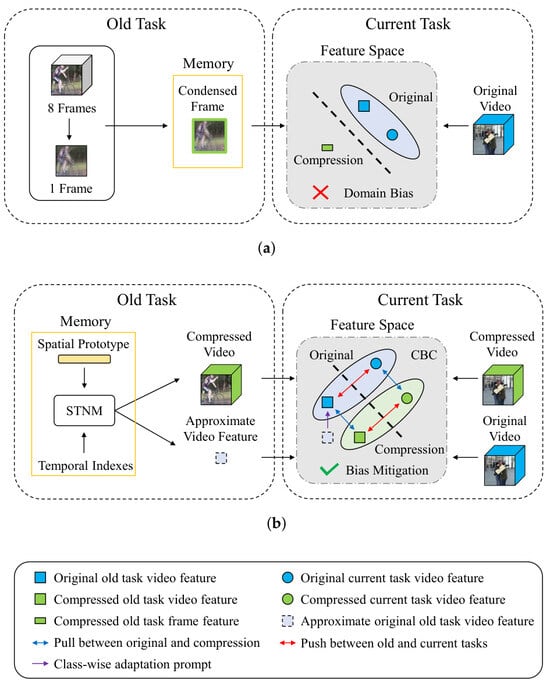
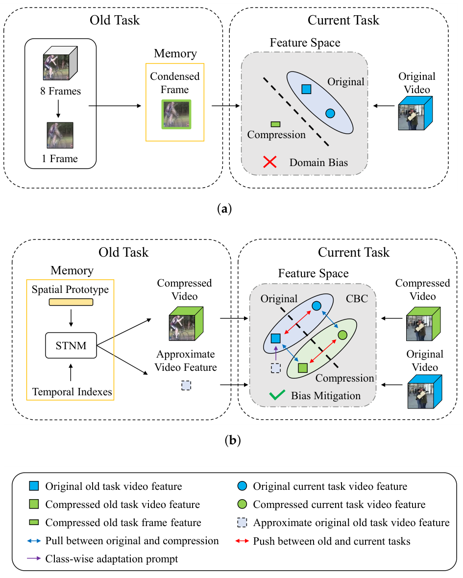
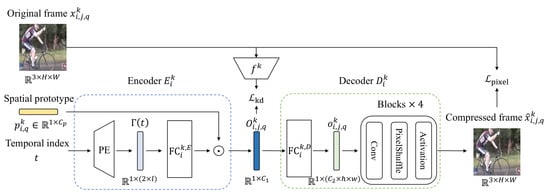
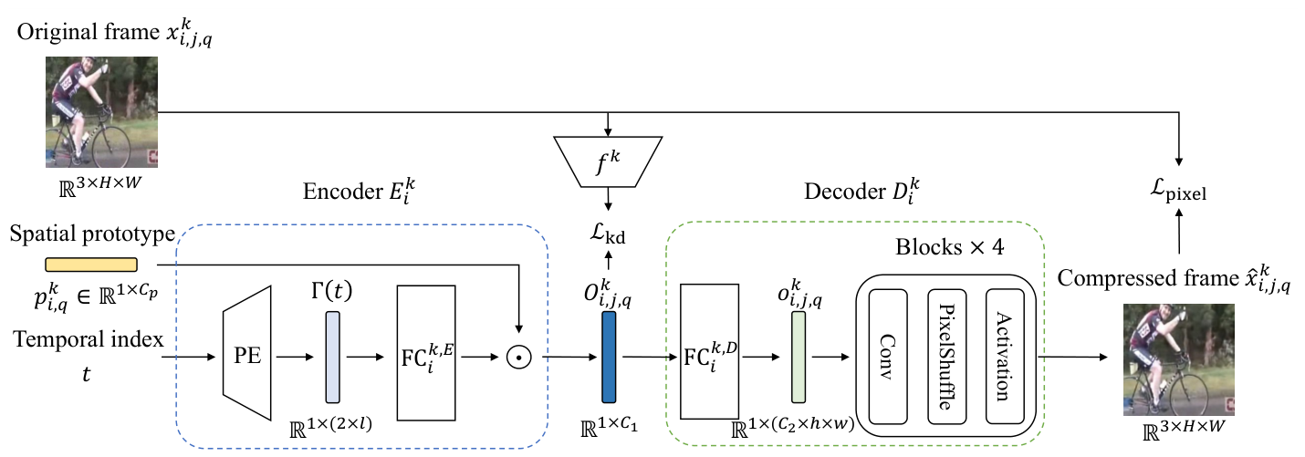
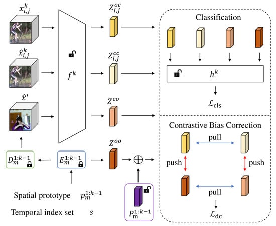
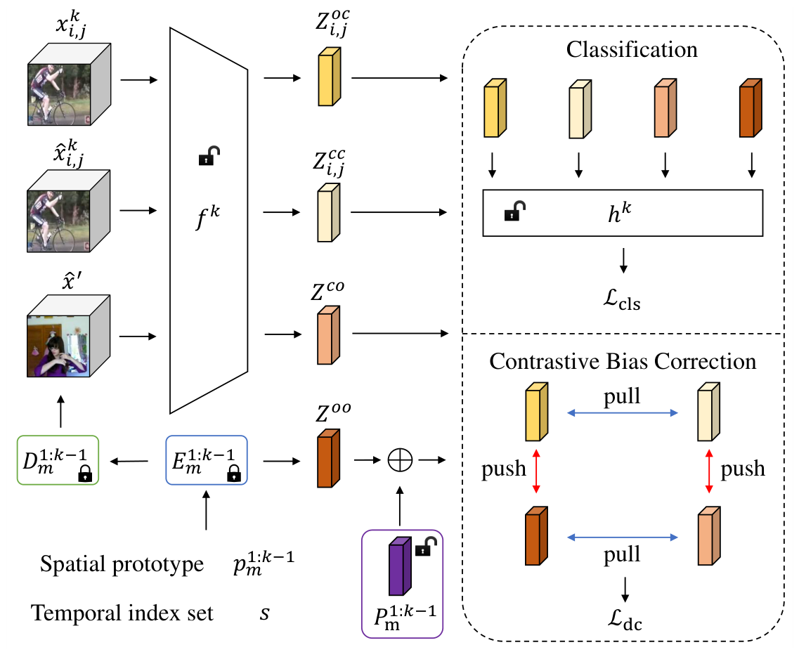
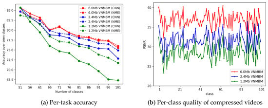
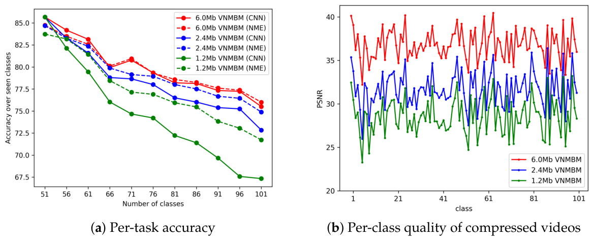
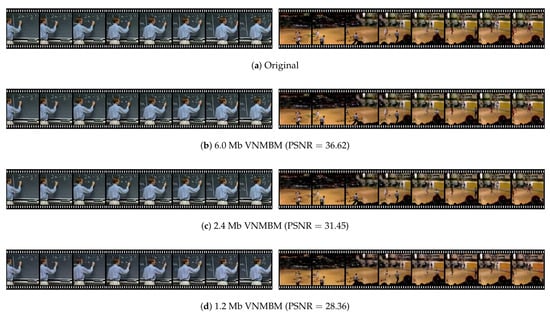
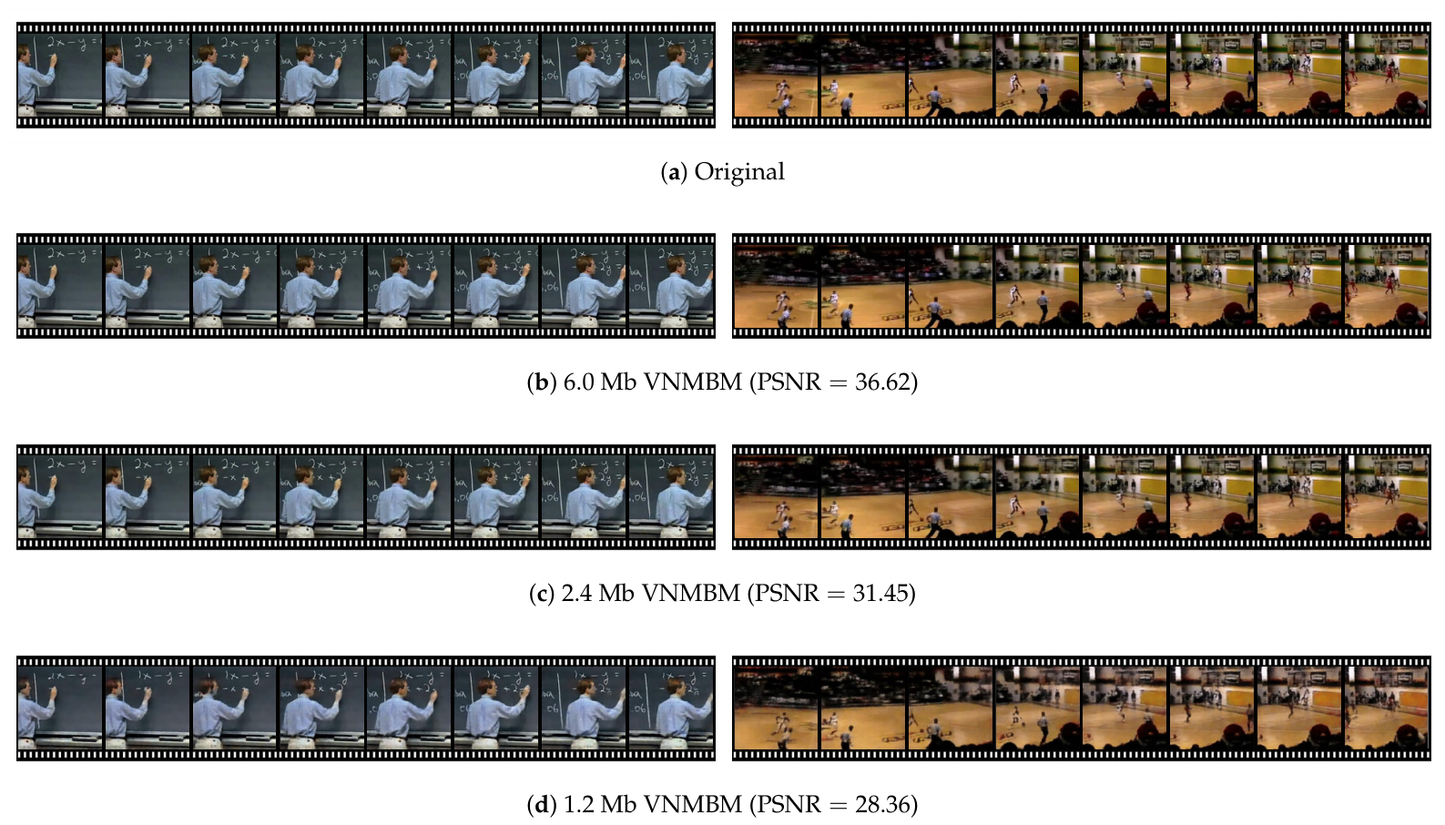
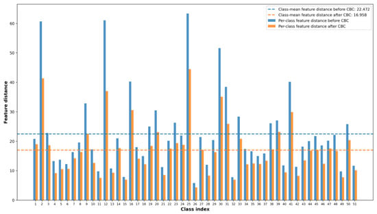
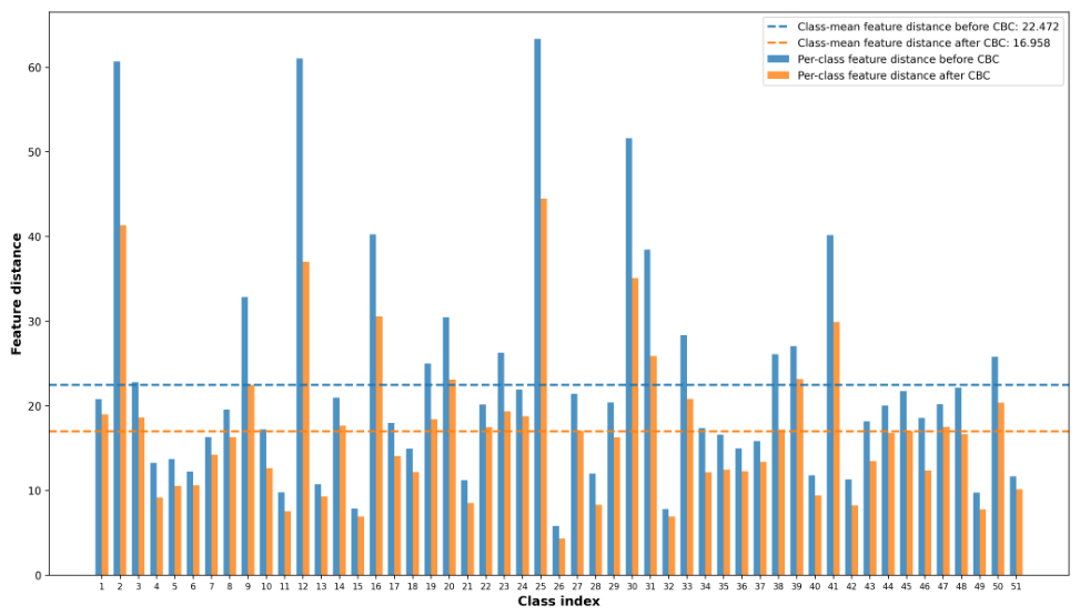
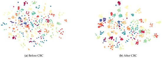
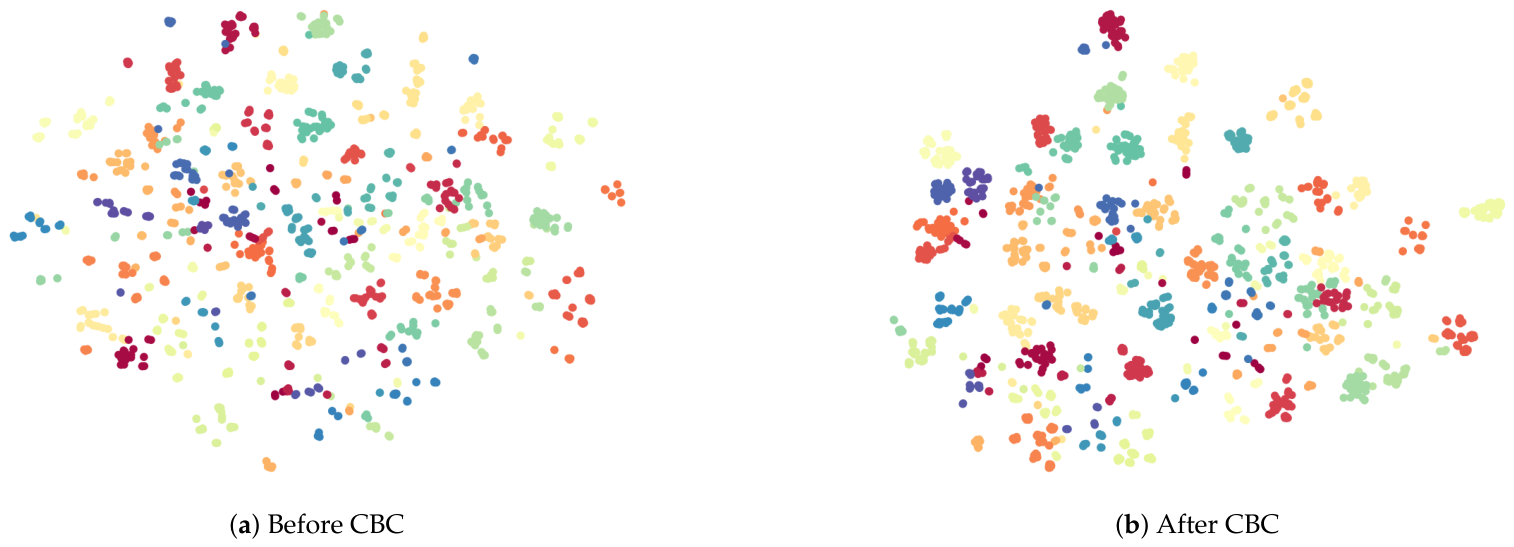
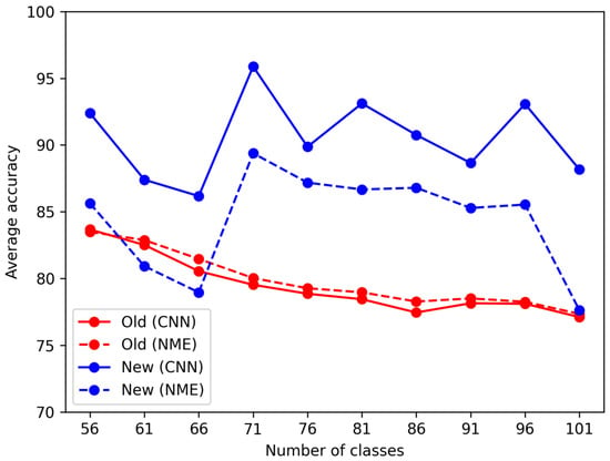
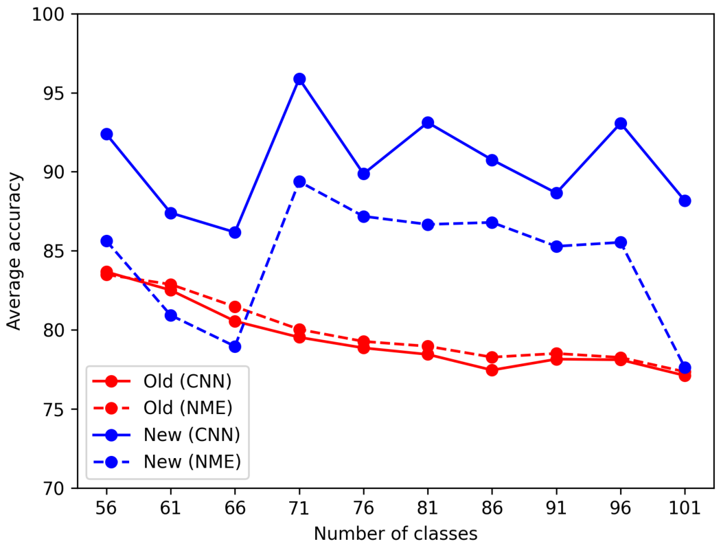

Disclaimer/Publisher’s Note: The statements, opinions and data contained in all publications are solely those of the individual author(s) and contributor(s) and not of MDPI and/or the editor(s). MDPI and/or the editor(s) disclaim responsibility for any injury to people or property resulting from any ideas, methods, instructions or products referred to in the content. |
© 2026 by the authors. Licensee MDPI, Basel, Switzerland. This article is an open access article distributed under the terms and conditions of the Creative Commons Attribution (CC BY) license.