An Evolving Fuzzy Belief Classification Technology for Bearing Fault Diagnosis

Abstract

Self-organizing fuzzy belief inference systems (SOFBISs) have been used in evolving prototype-based classifications. However, the existing SOFBIS models treat all features and statistical descriptors equally, which may limit their performance in applications where input features have unequal diagnostic relevance. This paper presents an evolving fuzzy belief (EFB) technique to enhance pattern classification and machine condition monitoring. Application of a new feature, Manhattan distance measure, is proposed to highlight informative features and suppress less relevant patterns. The feature weights are estimated using class-wise Pearson correlations to emphasize informative features, thereby improving the interpretability and accuracy of fault diagnosis. The effectiveness of the proposed EFB technique for bearing health condition monitoring and fault diagnosis is examined by both simulation and experimental tests.

1. Introduction

Rolling-element bearings are essential components in rotating machines. Up to 50% of malfunctions in rotating machines are related to bearing faults. Reliable bearing fault detection and diagnosis techniques and tools are critically needed in industries to improve machine operation quality, reliability and safety, as well as to reduce maintenance costs by avoiding periodically shutting down machines for manual inspections (i.e., preventive maintenance) [1,2]. Unfortunately, reliable bearing fault diagnosis remains a challenging task in this research and development field; it is because, being different from a gear or shaft, a bearing is a system consisting of an inner race, an outer race, rolling elements and a cage, each generating specific vibration signals. In addition, bearing fault-related features are relatively weak and modulated by other vibration signals. To address this issue, researchers have proposed many bearing fault detection methods in the time domain, frequency domain and time–frequency domain. But each of these techniques has its own merits and limitations [3]. One solution to improve bearing fault diagnostic reliability is to integrate the merits of several fault detection techniques for automatic bearing condition monitoring, using appropriate intelligent classifiers. The traditional intelligent classifiers use fixed classification structures such as support vector machines, K-nearest neighbors, and naive Bayes, which have limited adaptability in time-varying environments [3,4]. Fuzzy systems use fuzzy “If–Then” rules in pattern classification and diagnostic decision-making. Although fuzzy systems have merits such as transparency and interpretability in reasoning, traditional fuzzy inference systems (FIS) often rely on static rule bases and predefined reasoning structures designed by experts, which limit their adaptability in dynamic and time-varying environments [5]. Neuro-fuzzy (NF) models integrate fuzzy reasoning with neural network-based parameter training to improve adaptability while maintaining interpretability. However, they require large tr28aining datasets and are prone to degradation of performance with uncertain or incomplete training data [6]. Building upon traditional fuzzy logic and complementing the NF models, belief rule (BR) systems introduce belief degrees into fuzzy rules to characterize uncertainty and incomplete information inherent in real systems [7]. BR inference is usually undertaken on evidential reasoning that relies on Dempster–Shafer theory [8]. This integration can properly handle uncertain and incomplete information in decision-making processes. However, BR systems inherit structural rigidity from traditional fuzzy systems, as they rely on expert-defined rule bases and fixed parameters, which restrict their adaptability and scalability in real-time monitoring applications [9]. To tackle the limitations of FIS, NF and BR systems [10], especially in their structural rigidity and limited adaptability while preserving model transparency, evolving fuzzy systems (eFS) have been proposed to enable online adaptation of fuzzy rules and structures by incrementally learning from streaming data [11]. For example, evolving Takagi–Sugeno model (eTS) [12] is proposed to incrementally tune fuzzy rules based on data-driven estimation; however, it relies on predefined rule structures, which could be inefficient in highly dynamic data streams. Parsimonious fuzzy network [13] is suggested to support both structure and parameter adaptation. However, its open evolving mechanism makes it highly sensitive to data fluctuations and noise, especially in streaming environments. Dynamic evolving neural-fuzzy inference system (DENFIS) [14] can support online learning by combining supervised and unsupervised rule evolution and rule selection; however, its performance largely depends on the adequacy of training sample coverage over the input spaces. The authors’ research team has also proposed eFS techniques for dynamic system analysis [15] and machine condition monitoring [16]. Each of these classical eFSs has demonstrated its own strengths and limitations, which drive the development of more flexible and powerful classification frameworks for better interpretable, adaptive, and uncertainty-aware classifications, especially under real-world conditions [17]. While deep learning models such as convolutional neural networks, recurrent neural networks, and vision transformers have shown impressive performance in fault diagnosis, they lack transparency and require extensive training data. Recent intelligent fault-diagnosis studies have explored complementary challenges such as emerging fault recognition, interpretable diagnosis, and complex time–frequency dependency. For example, OpensetCapsNet [18] can jointly address emerging and compound faults through open-set recognition and capsule-based representation learning. The Traceable Algorithm Unrolling network [19] improves interpretability by embedding sparse-representation mechanisms into a deep diagnostic architecture. In addition, the time–frequency fully connected graph neural network [20] models multiscale spatiotemporal dependencies from multisource machinery signals. On the other hand, these methods generally rely on relatively complex deep architectures and extensive feature learning.

Some recent efforts have focused on integrating fuzzy rule-based reasoning with evolving learning mechanisms to enhance both interpretability and adaptability under streaming or scarce data conditions [6,21]. Among them, the self-organizing fuzzy belief inference system (SOFBIS) provides a promising method by combining Bayesian-style BRs with evolving fuzzy structures [22,23]. Unlike conventional fuzzy models, SOFBIS enables online incremental learning without predefined rule bases to handle interclass overlaps and multimodal data. Several recent works have extended the SOFBIS method to address complex streaming data scenarios. For example, a self-adaptive fuzzy learning ensemble system is suggested in [24] to integrate SOFBIS with ensemble pruning and dimensionality compression for flexible classification under concept drift and high-dimensional data streams. A prototype-based fuzzy classifier in [25] applies multi-objective evolutionary optimization to refine prototype placement to improve rule compactness. However, these methods have not considered the varying importance of input features in distance calculations, which limits their processing accuracy in redundant environment decision-making [26]. Some other evolutionary fuzzy systems have been adopted to explore different strategies to reduce rule complexity. For instance, the modified sequential adaptive fuzzy inference system in [27] addresses class imbalance using fuzzy clustering and generative modeling; an evolving fuzzy classifier is introduced [16] with participatory learning and a multivariable Gaussian method. However, these methods rely on uniform distance metrics and employ black-box inference mechanisms, which may limit their reasoning transparency when dealing with redundant and high-dimensional input spaces.

To tackle these problems, a new evolving fuzzy belief (EFB) classification technique is proposed in this work for more accurate pattern classification and bearing fault diagnosis. The EFB technique is new in the following aspects: (1) It introduces feature-weighted Manhattan distance measures into both training and inference processes. The feature weights are estimated from labeled training data using class-wise correlation analysis and incorporated into the Manhattan distance measure to emphasize diagnostically informative features. (2) The EFB technique is implemented for fault diagnosis of rolling-element bearings, and its effectiveness is validated by both simulation and experimental tests.

The remainder of this paper is organized as follows: Section 2 presents the proposed EFB technique. The effectiveness of the EFB technique is verified in Section 3 by simulation tests. Its effectiveness in bearing fault diagnosis is examined in Section 4 by simulation and experimental tests.

2. Proposed EFB Technique

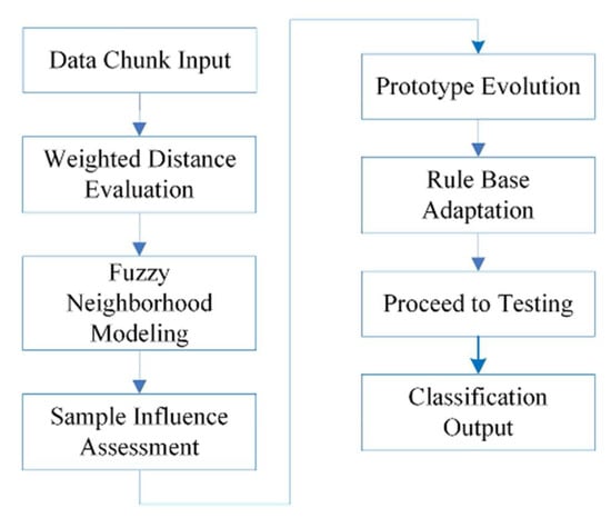
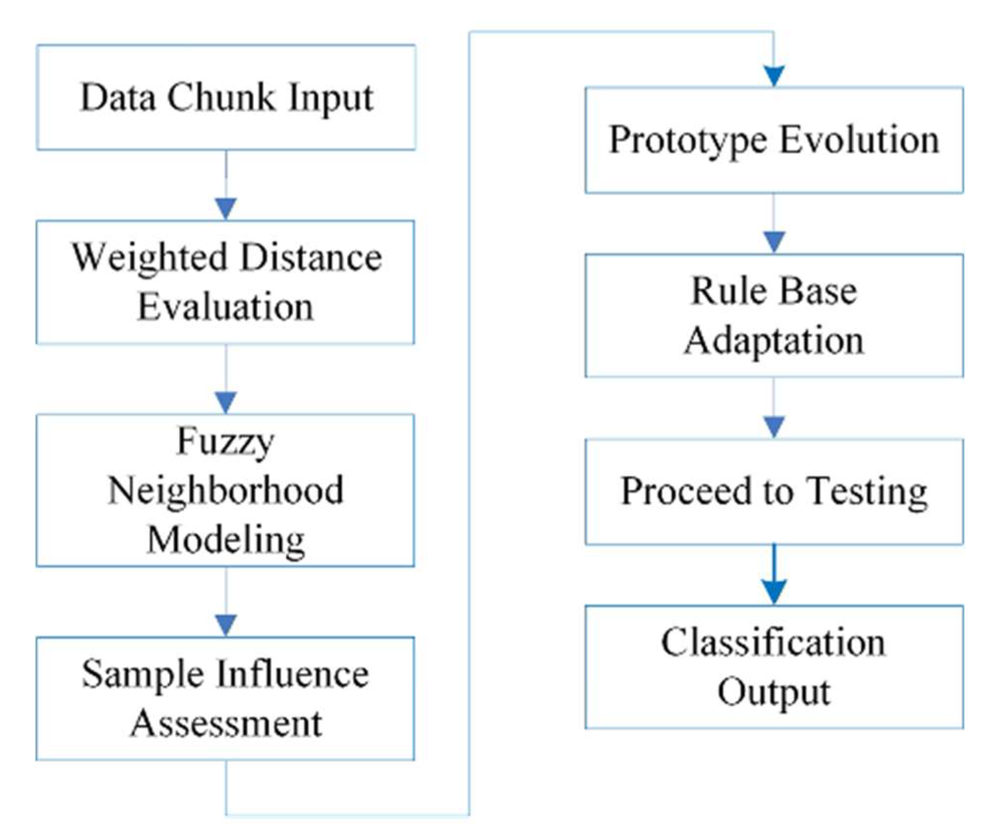
Figure 1 shows the flowchart of the proposed EFB technique. During the supervised training stage, each labeled training data chunk is first processed to compute feature similarities to recognize fuzzy neighborhoods. A set of representative prototypes are then generated through a support learning algorithm. During the test stage, new samples are classified using the learned prototypes and their corresponding fuzzy membership degrees, without requiring the true class labels of the test samples. Detailed processing will be discussed in the following subsections.

Figure 1. The flowchart of the proposed EFB technique.

2.1. EFB System Evolution

The proposed EFB classification technique operates on incoming data chunks. It follows a supervised evolving learning protocol. Labeled data chunks are used for feature-weight estimation and prototype evolution in training. During prediction, unseen samples are classified using the learned feature weights and prototypes without requiring their true class labels. Let X ∈ R^n×d denote an input data chunk with n samples and d features. Each sample is represented as x_i, i = 1, 2, …, n, and associated with a label y_i ∈ {1, 2, …, C}, where C represents the total number of classes.

For each labeled training data chunk X, the feature weights are estimated in training by measuring the relevance of each feature to the class labels. To avoid imposing an artificial ordinal relationship on nominal class labels, the multiclass labels are transformed into one-vs-rest binary class indicators. For each feature X_k, the absolute Pearson correlation is calculated for each binary class. The resulting class-wise correlations are averaged to obtain the feature weight w_k:

$$w_k={\displaystyle \frac{1}{C}}{\displaystyle \sum _{c=1}^C|\mathit{corr}(X_k,y_c)|}$$

(1)

where X_k ∈ Rⁿ is the k-th feature vector, C is the number of classes, y_c ∈ Rⁿ is the one-vs-rest binary indicator for class c; the i-th element equals 1 if y_i = c and 0 otherwise. The term corr(X_k, y_c) denotes the Pearson correlation coefficient between X_k and y_c.

The learned feature weights are subsequently used for class prediction, whereas test labels are not required during prediction. Given two samples x_i and x_j in the current chunk X, the weighted Manhattan distance between them is calculated as:

$$d(x_i,x_j)={\displaystyle \sum _{k=1}^{N_f}{w}_k\cdot \left|x_{i,k}-x_{j,k}\right|}$$

(2)

where N_f is the number of features and w_k denotes the weight of the k-th features.

To enable smooth neighborhood construction, a distance threshold τ is defined by averaging all pairwise weighted distances between samples in the current data chunk:

$$\tau ={\displaystyle \frac{1}{n(n-1)}}{\displaystyle \sum _{i=1}^n{\displaystyle \sum _{j=i+1}^{n}d(x_i,x_j)}}$$

(3)

where n is the number of samples in the current data chunk X. The estimated threshold τ provides an adaptive criterion for identifying neighborhood relationships within each data chunk. It reflects the overall distribution and dispersion of the samples in the current chunk to determine whether two samples are sufficiently close to be regarded as neighbors.

Based on this criterion, a binary adjacency matrix B ∈ R^n×n is defined to characterize the local neighborhood structure of the data. Specifically, the adjacency relationship between two samples x_i and x_j is defined as:

$$B_{i,j}=\left\{\begin{array}{c}1,\mathit{if}d(x_i,x_j)\le \tau \\ 0.\mathit{otherwise}\end{array}\right\}$$

(4)

Accordingly, two samples are considered adjacent if their pairwise distance satisfies the neighborhood threshold; otherwise, they are treated as non-neighbors.

Fuzzy membership degrees are introduced to characterize the relative influence between each data sample and its neighboring samples. Instead of employing the Gaussian-like decay function adopted in the SOFBIS [23], an inverse distance weighting measure is utilized to define the fuzzy membership matrix, which adaptively modulates neighborhood influence, without relying on predefined decay scales. Accordingly, the fuzzy membership matrix μ_i,j ∈ R^n×n is defined as:

$${\mu }_{i,j}=B_{i,j}\cdot {\displaystyle \frac{1}{d(x_i,x_j)+\epsilon }}$$

(5)

where μ_i,j is the fuzzy membership degree between samples x_i and x_j; d(x_i, x_j) denotes the weighted distance between them; and ε is a small positive constant used to avoid numerical instability when the distance approaches zero.

Based on the fuzzy membership matrix, the fuzzy neighborhood R(x_i) is defined as a set of samples within the current data chunk X with respect to x_i:

R(x_i) = {x_j ∈ X | μ_i,j > 0}

(6)

This fuzzy neighborhood formulation enables a soft representation of local sample relationships, enabling neighboring samples to contribute to subsequent prototype learning and rule generation adaptively.

To characterize the local representativeness of each sample within its fuzzy neighborhood, a relative fuzzy support measure is defined based on the fuzzy membership degrees between a sample and its neighboring samples. Given the fuzzy membership matrix μ quantifying the pairwise neighborhood influence among samples within the current data chunk, the fuzzy support of sample x_i is computed as:

$$r_i={\displaystyle \frac{{\displaystyle \sum _{j=1}^n{\mu }_{i,j}}}{{\displaystyle \sum _{i=1}^n{\displaystyle \sum _{j=1}^n{\mu }_{i,j}}}}}$$

(7)

where n is the number of samples; and r_i denotes the aggregated representative score of x_i, which quantifies its relative importance within the local fuzzy neighborhood.

Next, each sample is compared with the other samples within its fuzzy neighborhood. The sample x_i is selected as the primary prototype p_i if it achieves the maximum representative score r_i among all samples in its fuzzy neighborhood, which can be represented as:

IF r_i = max{r_k | x_k ∈ R(x_i)}, THEN p_i = x_i AND p_i ∈ P_t.

(8)

where R(x_i) represents the fuzzy neighborhood of sample x_i, and P_t denotes the set of primary candidate prototypes obtained from the current data chunk.

Based on the constructed fuzzy neighborhoods, representative samples are identified as prototypes to formulate the local data structure that preserves both the intrinsic feature characteristics and the associated class belief information. The geometric centers of the selected prototype candidates in P_t are updated to better represent the local data distribution. Specifically, for each prototype candidate x_i^(t) ∈ P_t, its updated center a_i^(t) is recognized as the average of its connected neighboring samples, such that

$$a_i^{(t)}={\displaystyle \frac{{\displaystyle {\sum }_{j=1}^{N_i}{B}_{i,j}^{(t)}B\cdot x_j^{(t)}}}{{\displaystyle {\sum }_{j=1}^{N_i}{B}_{i,j}^{(t)}}}}$$

(9)

where x_j^(t) is the j-th neighboring sample connected to x_i^(t); B_i,j^(t) denotes 1 or 0 indicating whether sample x_j^(t) is connected to prototype x_i^(t) or not, respectively; and N_i is the total number of connected neighbors of the prototype.

After updating the prototype centers, a belief vector is assigned to each prototype to characterize local class distribution within its neighborhood. Specifically, for a prototype p_i^(t), the belief vector β_i^(t) = [β_i,1^(t), …, β_i,C^(t)] is defined as

$${\beta }_{i,c}^{(t)}={\displaystyle \frac{{\displaystyle {\sum }_{j=1}^{N_i}{B}_{i,j}^{(t)}\delta (y_j^{(t)},c)}}{{\displaystyle {\sum }_{j=1}^{N_i}{B}_{i,j}^{(t)}}}}, c=1,\dots ,C,$$

(10)

where Δ(y_j^(t), c) equals 1 or 0 representing whether the class label of sample x_j belongs to c, or not, respectively.

This belief vector β_i^(t) reflects the relative class proportions of samples connected to the prototype. In addition, a support factor S_i^(t) is assigned to each prototype to characterize its representative grade within the current data chunk calculated by:

$$S_i^{(t)}={\displaystyle \sum _{j=1}^{N_t}{B}_{i,j}^{(t)}}$$

(11)

where N_t denotes the total number of samples in the current chunk t. The support factor S_i^(t) reflects the number of samples connected to the prototype.

Next, an adaptive distance threshold is introduced to determine whether a newly generated prototype should be retained as a distinct prototype or merged with existing ones. If t > 1, the kernel width λ is adaptively updated based on the measure of both the current and previous data chunks, such that:

$$\lambda \leftarrow \sqrt{{\displaystyle \frac{{\displaystyle {\sum }_{j=1}^{t-1}{N}_j{\lambda }^2+N_t{\sigma }_t^2}}{{\displaystyle {\sum }_{j=1}^t{N}_j}}}}$$

(12)

where N_j is the total number of samples in the j-th chunk; N_t is the number of samples in the current chunk t; and σ_t² is the estimated variance of the current chunk.

Based on the updated distance threshold λ, each newly generated prototype p_i^(t) ∈ P_t is compared with all existing prototypes. Specifically, the minimum Manhattan distance between p_i^(t) and the existing prototypes is defined as:

$$d_{\min }=\underset{j}{\min }{‖p_i^{(t)}-{\tilde{p}}_j‖}_1$$

(13)

where p_i^(t) is the i-th newly generated prototype obtained from the current data chunk; ${\tilde{p}}_j$ is the j-th existing prototype in the rule base; and the index j runs over all existing prototypes.

If d_min > λ, the prototype is added to the rule base together with its associated belief vector and support factor. Otherwise, if d_min ≤ λ, the prototype is merged with its closest existing prototype according to the updating rules discussed below.

Let v_i^(t) denote the belief vector with a newly generated prototype p_i^(t) from the current chunk, with the support factor s_i^(t). For an existing prototype ${\tilde{p}}_j$ in the rule base with corresponding belief vector ${\tilde{v}}_j$ and support factor ${\tilde{s}}_j$, respectively, when a newly generated prototype p_i^(t) is sufficiently close to an existing one or d_min ≤ λ, a prototype merging operation is performed to adaptively update the knowledge base. Specifically, the belief vector of the existing prototype is updated by:

$${\tilde{v}}_j\leftarrow {\tilde{v}}_j+{\displaystyle \frac{s_j^{(t)}}{s_j+s_i^{(t)}}}(v_i^{(t)}-{\tilde{v}}_j).$$

(14)

The support value of the existing prototype is updated as

$$s_j\leftarrow s_j+s_i^{(t)}$$

(15)

Using the above adaptive prototype merging approach, the rule base is adaptively updated, with each prototype acting as a fuzzy rule characterized by its center a_i^(t). After each data chunk is processed, the updated prototypes P_t, their corresponding belief vectors β_i^(t) and support factor S_i^(t) are employed in class prediction, as discussed below.

2.2. Class Prediction

During the class prediction stage, the proposed EFB technique performs classification by evaluating the relationship between a new test sample and the existing prototypes. For a given test sample x, the weighted distance between x and each existing prototype p_j is first computed according to Equation (2). Then the adaptive neighborhood membership degree between the test sample and each prototype, μ_j(x), is estimated using Equation (5). Each prototype p_j is associated with a belief vector β_j that represents the class distribution. Then, the cumulative confidence score for class c is computed as

$$S(c|x)={\displaystyle {\sum }_{j=1}^{C_L}{\mu }_j(x){\beta }_{j,c}}$$

(16)

where C_L is the total number of existing prototypes; μ_j(x) denotes the soft membership degree between the test sample and prototype p_j; and β_j,c is the belief of prototype p_j supporting class c.

The predicted class label of the test sample is then determined by selecting the class that yields the maximum cumulative confidence score:

$$\widehat{y}=\arg \underset{c}{\max }S(c|x)$$

(17)

This class prediction process relies on the joint activation of prototype-based fuzzy membership degrees and their associated belief distributions, which enables an interpretable classification process. Each prototype–belief pair can be viewed as a fuzzy rule characterizing a local region of the feature space.

3. Performance Evaluation Based on Simulation Tests

First, the effectiveness and generalization capability of the proposed EFB technique are evaluated through simulation tests using some benchmark datasets under different data sizes, numbers of features and class distributions.

3.1. Benchmark Dataset Illustration

In this study, four commonly used benchmark datasets with different characteristics are used to evaluate the classification performance of the proposed EFB technique. For all datasets, the input variables correspond to the feature vectors, while the output labels represent the associated class categories. The Iris dataset [28] comprises 150 samples described by four floral features, namely sepal length, sepal width, petal length, and petal width, and involves three flower species as output classes. The Wine dataset [29] contains 178 samples with 13 physicochemical features and three output classes, which will be used to evaluate classification performance under high-dimensional feature spaces. The Wisconsin Breast Cancer dataset [30] includes 699 samples characterized by nine cytological features and aims to distinguish between benign and malignant tumors. The Pima Indians Diabetes dataset [31] comprises 768 samples with eight diagnostic features and exhibits class imbalance and overlapping distributions, which poses a more challenging classification task.

3.2. Benchmark Results and Interpretability Analysis

To evaluate the performance of the proposed EFB technique, three related evolving fuzzy classification techniques are used as baseline methods for comparison, including SOFIS+ [26], ALMMo1 [32], and SOFBIS [23]. These methods represent different modeling paradigms in evolving fuzzy systems, enabling a balanced evaluation of the proposed EFB approach. Specifically, SOFIS+ is a zero-order self-organizing fuzzy inference ensemble system that incrementally constructs fuzzy rules from data streams and combines them through an ensemble learning strategy. ALMMo1 is a first-order autonomous learning multi-model system that dynamically generates, updates, and prunes local models to adapt to data distributions in streaming environments. SOFBIS+ is a belief-rule prototype-based fuzzy inference system that integrates fuzzy logic with belief-rule reasoning to model uncertainty and class evidence. These baseline methods cover zero-order, first-order, and belief-rule-based fuzzy modeling structures, ensuring a diverse and representative comparison. All methods are implemented and evaluated in MATLAB R2022b within a unified processing framework using consistent data preprocessing procedures and 5-fold cross-validation settings. For each cross-validation fold, the input features are normalized over [0, 1] using min–max scaling. The minimum and maximum values of each feature are estimated exclusively from the training set, and the same scaling parameters are subsequently applied to the corresponding test set to avoid information leakage.

Table 1 summarizes the classification accuracy of the related classification techniques. It is seen that the EFB technique achieves the highest classification accuracy among all baseline methods, which can be attributed to its adaptive feature-weighting strategy.

Table 1. Classification accuracy (%) on benchmark datasets.

Dataset	SOFIS+ (%)	ALMMo1 (%)	SOFBIS (%)	EFB (%)
IRIS	94.93	82.22	94.60	95.13
Wine	96.63	96.23	97.60	96.01
Cancer	96.40	95.59	96.50	96.76
Pima	70.77	72.61	72.62	75.27
Mean	89.68	86.66	90.33	90.79
SD	12.63	11.38	11.87	10.37
CV	14.08	13.13	13.14	11.42

EFB also achieves the highest mean accuracy of 90.79%, together with the lowest standard deviation (SD) of 10.37% and coefficient of variation (CV) of 11.42%, indicating better overall consistency across the four benchmark datasets.

To further investigate the effect of involved components in EFB, an ablation study is conducted using the same benchmark datasets and the same cross-validation settings. Starting from the baseline configuration, adaptive feature-weighting, inverse-distance membership, and modified prototype generation/evolution mechanism are introduced progressively. The corresponding results are summarized in Table 2. It is seen that adaptive feature-weighting provides a significant contribution to the observed performance improvement, increasing the mean accuracy from 88.93% to 90.84%. The inverse-distance formulation does not provide clear improvement on the benchmark datasets when it is used alone. However, the complete EFB framework achieves the highest mean accuracy of 90.99%, together with the lowest SD of 10.51% and CV of 11.55%.

Table 2. Classification accuracy (%) of the ablation study on benchmark datasets.

Dataset	Baseline	+Weighting	+Weighting + InvDist	EFB
IRIS	94.80	95.00	94.73	95.13
Wine	95.15	96.63	95.23	96.62
Cancer	96.59	96.95	95.34	96.93
Pima	69.18	74.77	72.61	75.27
Mean	88.93	90.84	89.48	90.99
SD	13.19	10.75	11.25	10.51
CV	14.83	11.83	12.57	11.55

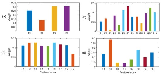
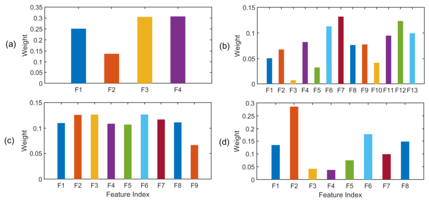
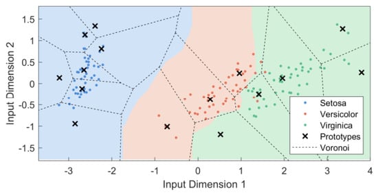
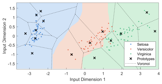
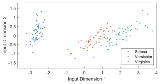
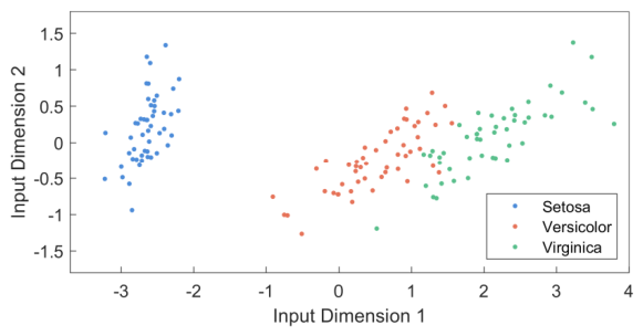
Figure 2 illustrates the corresponding adaptive feature weights from the EFB technique. Figure 2a shows the corresponding adaptive feature weights in Iris dataset classification. The adaptive feature-weighting strategy of the EFB technique can provide more discriminative petal-related features. Figure 3 presents a principal component analysis projection of the overall class distribution for the Iris dataset. Partial overlap exists between Versicolor and Virginica classes, posing a moderate challenge for multi-class classification. Figure 4 illustrates the classification regions generated by the proposed EFB technique. The resulting prototypes can formulate localized and well-structured decision boundaries, enabling effective discrimination in overlapping regions.

Figure 2. Feature weight learned by EFB from four benchmark datasets: (a) IRIS, (b) Wine, (c) Cancer, and (d) Pima.

Figure 3. Principal component analysis projection of the Iris dataset.

Figure 4. Visualization of the EFB classification result on the Iris dataset.

The Wine dataset has the characteristics of a relatively high-dimensional feature space with 13 physicochemical attributes. EFB attains an accuracy of 96.62%, outperforming all baseline methods. As shown in Figure 2b, the learned feature weights highlight informative variables such as alcohol content and flavonoids, while suppressing less relevant attributes.

The Wisconsin Breast Cancer dataset is comparatively clean and well-balanced. EFB exhibits performance comparable to SOFBIS and slightly superior to ALMMo1. The distribution of feature weights in Figure 2c suggests that most cytological features contribute meaningful information to malignancy discrimination, explaining the relatively small performance differences among competing methods.

The Pima Indians Diabetes dataset presents a more challenging classification scenario due to significant class imbalance and overlapping feature distributions. Under these conditions, EFB outperforms SOFIS+, ALMMo1 and SOFBIS, respectively. As illustrated in Figure 2d, dominant weights are associated with glucose and body mass index, which are clearly recognized as key diagnostic indicators, thereby enhancing robustness under imbalanced data conditions.

From the above results and analysis, it is seen that the proposed EFB classifier can adapt to diverse data characteristics—including low-dimensional overlapping classes, high-dimensional feature spaces, balanced datasets, and imbalanced scenarios—while providing interpretable insights of classification processing. This combination of performance and interpretability recommends it for application in real-world bearing condition monitoring discussed in the following section.

4. Performance Evaluation for Bearing Fault Diagnosis

The effectiveness of the proposed EFB technique will be evaluated for bearing health condition monitoring and fault diagnosis. Its effectiveness, including robustness, is evaluated experimentally in this section.

4.1. Laboratory Bearing Condition Monitoring

4.1.1. Experimental Setup

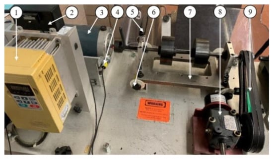
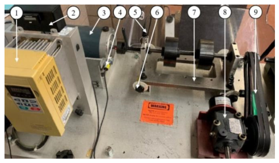
Figure 5 shows the experimental setup used in this test. It is driven by a 3 HP induction motor with a speed range of 100 ~ 4200 rpm, controlled by a frequency converter (VFD022B21A). An elastic coupler is applied to eliminate high-frequency vibrations generated by the motor. An optical sensor is used to provide a signal of one pulse per revolution to measure shaft speed, which is inputted into the monitoring system. The accelerometers (ICP-603C01) are mounted on the top and back of the bearing housing to measure the vibration signal along the vertical and horizontal axes. Redundant sensor information can be used not only for processing result verification, but also for sensor and connection integrity assessments [33]. The vibration signals are fed to a computer through a smart data acquisition (DAQ) system developed by our research team. The smart wireless DAQ system is a 4-channel distributed measurement system that collects sensor signals, digitizes them, processes the data, and transmits the measurements wirelessly to a computer or central monitoring station. It uses both an FPGA and a microcontroller for processing. The FPGA provides high-speed, deterministic data acquisition, while the microcontroller handles sensor interfacing, system control, wireless communication, and power management. Its ADC resolution is 24 bits using external ADC chips, with a sampling rate up to 100 kS/s per channel over four channels.

Figure 5. Experimental setup: (1) speed controller; (2) encoder display; (3) drive motor; (4) optical encoder; (5) ICP accelerometer; (6) misalignment adjustor; (7) adjustable rig; (8) variable load system; (9) belt drive.

The tested bearing MBER-10K [34] is located in the left bearing housing. The static bearing load is provided by two heavy mass discs and dynamic load is provided by a brake system through a belt-drive.

A series of data sets have been collected from multiple accelerometers mounted on both sides of the bearing housing. The tests are conducted corresponding to different bearing health conditions: healthy bearings, bearings with outer race, inner race and rolling-element defects, respectively. The defect dimension (in diameter × depth) is: 0.3 mm × 0.3 mm (outer race defect), 0.3 mm × 0.3 mm (inner race defect), and 0.5 mm × 0.5 mm (ball defect), respectively.

The tests are undertaken under conditions of 100~4200 rpm, and 0.5~2 Nm operating conditions. If a bearing is damaged, the fault usually propagates slowly. Thus, condition monitoring is not conducted continuously, but every 15 min. The sampling frequency is selected based on shaft speeds. For example, if shaft speed is over 500~1000 rpm: f_s = 10,240 Hz; if shaft speed is over 1000~2000 rpm: f_s = 20,480 Hz; if shaft speed is over 2000–3000 rpm: f_s = 30,720 Hz. Each data collection is over 5 s; the collected vibration signals are divided into consecutive non-overlapping segments, each containing 30 shaft revolutions.

4.1.2. Input–Output Features

As stated in the Introduction, although there are many bearing fault detection methods proposed in the literature in the time domain, frequency domain and time–frequency domain, each method has its own merits and limitations and can be used for specific applications only [3]. It is mainly because the bearing is a complex system and its fault-related features are relatively weak and modulated by other vibration signals. The proposed EFB classifier will integrate the merits of several robust techniques for more reliable bearing fault diagnosis. The selected features should be robust in monitoring applications, or sensitive to bearing fault but insensitive to noise. By systematic investigation, the three selected features originate from signal processing techniques of the statistical kurtosis, the Hilbert–Huang Transform (HHT) [35], and the squared envelope spectrum (SES) [36], which are employed as inputs to the classifiers. Detailed discussions about the time response and frequency response of the related bearing faults, as well as the related dynamics analysis, can be found in [3].

The output of the classifier corresponds to bearing health conditions, including healthy and fault conditions, where fault condition is further classified into outer race defect, inner race damage, and rolling-element fault. Before classification, the extracted features are normalized using the same training set-based min–max procedure described in Section 3.2, to ensure comparable numerical scales among different types of features.

For HHT-based feature extraction, empirical mode decomposition is applied to each vibration segment, and three intrinsic mode functions with the highest kurtosis values are selected. The Hilbert marginal spectrum was calculated over 0–400 Hz with a frequency resolution of 0.5 Hz. For SES-based feature extraction, the signals are detrended and bandpass-filtered at 2–8 kHz. The spectral amplitudes at the selected characteristic frequencies and their first three harmonics are integrated for analysis.

The same baseline methods as used in Section 3.2: SOFIS, ALMMo1 and SOFBIS, are also applied in this test for comparison. All processing is conducted in MATLAB R2023b, and five-fold cross-validation is applied to ensure statistical reliability. The reported accuracy reflects the average performance across the five folds.

4.1.3. Experimental Test Results and Discussion

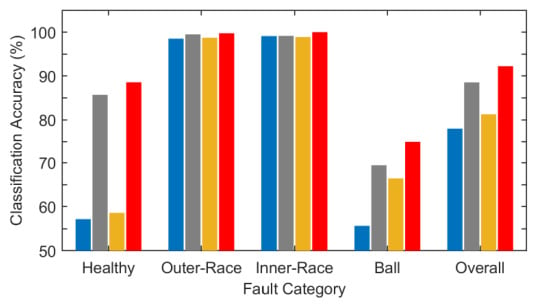
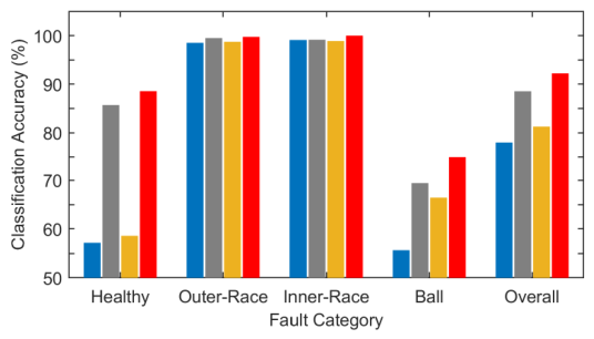
Table 3 summarizes the diagnostic classification accuracy using the related techniques, while Figure 6 provides a visual comparison of the classification performance across different fault categories.

Table 3. Classification accuracy on laboratory data.

Health Condition	SOFIS+ (%)	ALMMo1 (%)	SOFBIS (%)	EFB (%)
Healthy	53.19	83.24	57.23	84.12
Outer race	97.32	98.05	97.86	98.46
Inner race	98.23	98.68	98.12	98.73
Ball fault	49.69	50.98	55.43	57.11
Mean	74.61	82.74	77.14	84.61
SD	26.79	22.34	24.09	19.56
CV	35.91	27.00	31.23	23.12

Figure 6. Diagnostic classification accuracy comparison using the related techniques: SOFIS+ (blue), ALMMo1 (gray), SOFBIS (yellow), and the proposed EFB technique (red), respectively.

As summarized in Table 3 and illustrated in Figure 6, the proposed EFB technique consistently achieves the highest classification accuracy across all bearing health conditions. EFB exhibits strong discrimination capability for the outer-race and inner-race fault conditions, with accuracy reaching approximately 98.73%. EFB achieves the highest mean accuracy of 84.61%, with the lowest SD of 19.56% and CV of 23.12%, indicating better overall consistency across the four bearing health conditions. On the other hand, for the healthy bearing condition, the characteristic frequency is the shaft speed, whose harmonics are close to those spectral components from other vibration sources. As a result, the false diagnosis rate increases. When a rolling element (a ball in this case) is damaged, the impact feature properties become time-variant. The damaged location may not always strike the bearing’s outer race and/or the inner race due to the change in alignment of the damaged location. Correspondingly, all classifiers have much lower diagnostic accuracy. As a matter of fact, reliable ball fault detection remains a challenging task in this research and development field.

Compared with these baseline methods, the performance of EFB is most pronounced for the ball fault condition, indicating its effectiveness in handling fault types with relatively weak or complex diagnostic signatures. Overall, EFB outperforms other related classification techniques, demonstrating its clear advantage as an evolving fuzzy system in bearing health condition monitoring and fault diagnosis.

4.2. Robustness Evaluation

To further evaluate the robustness of the proposed EFB technique, more tests will be undertaken using the CWRU bearing dataset [37] under different bearing health states and test conditions, with results compared against the same baseline methods.

4.2.1. CWRU Experimental Setup

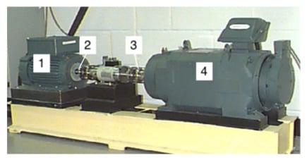
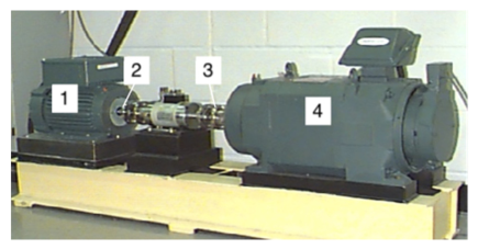
Figure 7 shows the experimental setup used in this study from the CWRU Bearing Data Center. It is driven by a 2 HP drive motor, and the load is provided by the load motor on the right. The tested bearing is installed in the bearing housing between the drive motor and the load motor. Vibration signals are collected using accelerometers.

Figure 7. CWRU bearing test experiment setup [37]: (1) electric motor, (2) drive end bearing, (3) torque sensor encoder, (4) dynamometer.

The tested bearing model is 6205-2RS JEM SKF (deep groove ball bearing) [38]. Under this experimental setup, vibration signals were collected under four different load conditions of 0, 1, 2, and 3 HP, corresponding to motor speeds of approximately 1797, 1772, 1750, and 1730 rpm, respectively. For each operating condition, four bearing health states are considered, including healthy, outer-race fault, inner-race fault, and rolling-element fault conditions. All faulty bearings have a single-point fault with a diameter of 0.007 in on the outer race, the inner race or the ball. The outer-race fault located at the centered 6:00 position is used. All fault-related vibration signals are collected from the drive end bearing dataset, with a sampling frequency of 48 kHz. The baseline healthy bearing vibration signals are acquired separately from the Normal Baseline Data subset under the same motor load conditions to ensure consistency. The vibration signals are segmented according to shaft revolutions. The number of samples per revolution is calculated as N_rev = round (f_s/f_r) where f_s is the sampling frequency and f_r is the shaft rotational frequency. Each segment contains 20 shaft revolutions, and consecutive non-overlapping segments are used. After segmentation and feature extraction, the datasets under 0, 1, 2, and 3 HP contain 75, 146, 146, and 145 classifier samples, respectively.

For consistency, the same inputs and outputs as described in Section 4.1.2 are used in the related classifiers. The classification experiments are conducted separately for each load condition using five-fold cross-validation repeated for 10 trials. To assess the influence of data partitioning, an additional chronological holdout experiment is conducted. For each bearing health condition, the first 70% of temporally ordered segments are used for training, approximately 10% are excluded as a separation gap, and the remaining segments are used for testing. This procedure reduces the direct mixing of neighboring segments between training and testing sets. The EFB data-block size is set to 30 samples, and the granularity level is set to 6. Specifically, fault-related features extracted from vibration signals using kurtosis, SES, and HHT techniques are employed as classifier inputs, while the outputs correspond to four bearing health conditions: healthy, outer-race fault, inner-race fault, and rolling-element fault. Different from the test in Section 4.1, the classification performance will be evaluated separately under the four load conditions, which provides a more challenging setting for evaluating the robustness of the proposed EFB classifier.

4.2.2. Test Results Analysis

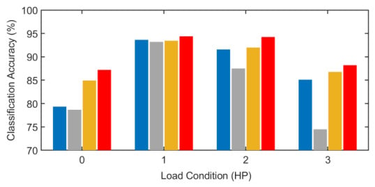
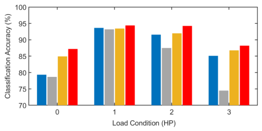
Table 4 summarizes the classification accuracies using the related classification techniques under four load conditions, and Figure 8 provides a visual comparison of their performance. It is seen that EFB maintains competitive classification performance across varying loads, with accuracies ranging from 87.03% to 94.32%. In comparison, the baseline methods exhibit variant variant performance as the load changes, especially under low (0 HP) and high (3 HP) load conditions.

Table 4. Classification accuracy under four load conditions on the CWRU bearing dataset.

Load (HP)	Speed (rpm)	SOFIS+ (%)	ALMMo1 (%)	SOFBIS (%)	EFB (%)
0	1797	79.33	78.67	84.93	87.20
1	1772	93.64	93.20	93.44	94.32
2	1750	91.57	87.50	91.98	92.58
3	1730	85.10	74.48	86.78	87.03
Mean	-	87.41	83.46	89.28	90.28
SD	-	6.50	8.46	4.07	3.73%
CV (%)	-	7.44	10.14	4.56	4.13%

Figure 8. Diagnostic classification accuracy comparison under four load conditions using the related techniques: SOFIS+ (blue), ALMMo1 (gray), SOFBIS (yellow), and the proposed EFB technique (red), respectively.

As summarized in Table 4, EFB achieves the highest mean accuracy of 90.28%, together with the lowest SD of 3.73% and CV of 4.13%, demonstrating better performance consistency across varying load and speed conditions. It is seen that EFB maintains competitive classification performance across varying loads, with accuracies ranging from 87.03% to 94.32%. In comparison, the baseline methods exhibit more variant performance as the load changes, especially under low (0 HP) and high (3 HP) load conditions. As summarized in Table 4, EFB achieves the highest mean accuracy of 90.28%, but the lowest SD of 3.73% and CV of 4.13%, demonstrating better performance consistency across varying load and speed conditions.

Table 5 compares the classification performance under random five-fold cross-validation and chronological holdout evaluation. The results show comparable accuracies across the four load conditions, with differences within 2.32%. This suggests that EFB maintains reasonable classification performance under temporal data separation. However, this evaluation does not fully eliminate within-recording correlations or establish generalization to independent recordings.

Table 5. Comparison of random five-fold cross-validation and chronological holdout evaluation on the CWRU dataset.

Load (HP)	Random-5-Fold (%)	Chronological Holdout (%)	Balanced Accuracy (%)
0	87.01	86.67	87.33
1	94.57	96.67	95.83
2	92.03	90.04	87.50
3	87.57	89.89	89.58

5. Conclusions

Rolling bearings are widely used in rotating machines, but their reliable fault diagnosis remains a challenging task in this research and development field due to their complex signal properties and signal modulations. An evolving fuzzy belief (EFB) technique has been proposed in this study for bearing condition monitoring and fault diagnosis. Application of a new feature, Manhattan distance measure, is suggested in the inference process to highlight informative features and suppress less relevant patterns. The prototype-based fuzzy reasoning is integrated with adaptive feature-weighting to achieve interpretable and more accurate fault classification diagnosis. The EFB technique has also been evaluated for bearing health condition monitoring and fault diagnosis using laboratory and CWRU datasets. The experimental results demonstrate competitive classification performance across different bearing health states and operating conditions. Its effectiveness has been verified by simulation and experimental tests. Test results show that EFB outperforms some related evolutionary fuzzy systems (e.g., SOFIS+, ALMMo1, and SOFBIS) in terms of accuracy and stability. It demonstrates potential for practical machine-condition-monitoring applications.

Advanced research was undertaken to further improve the accuracy of the proposed EFB technique, and to compare its effectiveness with other related classification techniques, including representative non-fuzzy classifiers under different bearing health states and operating conditions.

References

- Zhao, J.; Wang, W.; Huang, J.; Ma, X. A comprehensive review of deep learning-based fault diagnosis approaches for rolling bearings: Advancements and challenges. AIP Adv. 2025, 15, 020702. [Google Scholar] [CrossRef] [Scilit]
- Yan, X.; Li, N.; Nan, S.; Yu, Y.; Dai, R. A bearing fault diagnosis method for complex system based on improved extended belief rule base. Sci. Rep. 2026, 16, 15827. [Google Scholar] [CrossRef] [Scilit] [PubMed]
- Wang, W. Analysis of fault detection in rolling element bearings. IEEE Instrum. Meas. Mag. 2021, 24, 42–49. [Google Scholar] [CrossRef] [Scilit]
- Tian, J.; Morillo, C.; Azarian, M.H.; Pecht, M. Motor Bearing Fault Detection Using Spectral Kurtosis-Based Feature Extraction Coupled With K-Nearest Neighbor Distance Analysis. IEEE Trans. Ind. Electron. 2016, 63, 1793–1803. [Google Scholar] [CrossRef] [Scilit]
- Barai, V.; Ramteke, S.; Dhanalkotwar, V.; Nagmote, Y. Bearing fault diagnosis using signal processing and machine learning techniques: A review. IOP Conf. Ser. Mater. Sci. Eng. 2022, 1259, 012034. [Google Scholar] [CrossRef] [Scilit]
- Gu, X.; Ni, Q.; Shen, Q. Multilayer evolving fuzzy neural networks with self-adaptive dimensionality compression for high-dimensional data classification. IEEE Trans. Fuzzy Syst. 2024, 32, 6314–6328. [Google Scholar] [CrossRef] [Scilit]
- Toky, T.D.; Zhang, M.; Wang, W. An adaptive NF technology for bearing condition monitoring and fault diagnosis. Intell. Control Autom. 2025, 16, 61–79. [Google Scholar]
- Yan, X.; Li, N.; Yu, Y.; He, W.; Wang, D. A bearing fault diagnosis method based on hierarchical belief rule base with power set. IEEE Access 2025, 13, 70324–70339. [Google Scholar] [CrossRef] [Scilit]
- Yang, J.; Liu, J.; Wang, J.; Si, H.; Wang, H. Belief rule-base inference methodology using the evidential reasoning approach–RIMER. IEEE Trans. Syst. 2006, 36, 266–285. [Google Scholar] [CrossRef] [Scilit]
- Ming, Z.; Zhou, Z.; Hu, C.; Feng, Z.; Lian, Z.; Zhang, C. A new compact belief rule model for fault diagnosis. Control Eng. Pract. 2025, 159, 106298. [Google Scholar] [CrossRef] [Scilit]
- Gu, X.; Shen, Q. A self-adaptive fuzzy learning system for streaming data prediction. Inf. Sci. 2021, 579, 623–647. [Google Scholar] [CrossRef] [Scilit]
- Angelov, P.; Filev, D. An approach to online identification of Takagi–Sugeno fuzzy models. IEEE Trans. Syst. 2004, 34, 484–498. [Google Scholar] [CrossRef] [Scilit] [PubMed]
- Pratama, M.; Anavatti, S.; Angelov, P.; Lughpfer, E. PANFIS: A novel incremental learning machine. IEEE Trans. Neural Netw. Learn. Syst. 2014, 25, 55–68. [Google Scholar] [CrossRef] [Scilit] [PubMed]
- Kasabov, N.K.; Song, Q. DENFIS: Dynamic evolving neural-fuzzy inference system and its application for time-series prediction. IEEE Trans. Fuzzy Syst. 2002, 10, 144–154. [Google Scholar] [CrossRef] [Scilit]
- Ahwiadi, M.; Wang, W. An adaptive evolving fuzzy technique for prognosis of dynamic systems. IEEE Trans. Fuzzy Syst. 2022, 30, 841–849. [Google Scholar] [CrossRef] [Scilit]
- Shah, J.; Wang, W. An evolving NF classifier for fault diagnosis of gear systems. ISA Trans. 2022, 123, 372–380. [Google Scholar] [CrossRef] [Scilit] [PubMed]
- Gu, X.; Han, J.; Shen, Q.; Angelov, P. Autonomous learning for fuzzy systems: A review. Artif. Intell. Rev. 2023, 56, 7549–7595. [Google Scholar] [CrossRef] [Scilit]
- Huang, R.; Chen, Y.; Liu, C. OpensetCapsNet: A collaborative fault diagnosis framework for emerging and compound faults of machinery. ASCE-ASME J. Risk Uncertain. Eng. Syst. Part A Civ. Eng. 2026, 12, 4. [Google Scholar] [CrossRef] [Scilit]
- Lan, H.; Chen, Z.; Deng, S.; Huang, R.; Tsung, F.; Li, W. Traceable algorithm unrolling network: An interpretable deep sparse representation model for mechanical fault diagnosis. IEEE Trans. Cybern. 2026, 56, 927–939. [Google Scholar] [CrossRef] [Scilit] [PubMed]
- Xu, Y.; Li, S.; Li, Z.; Wu, K.; Huang, R.; Sun, B.; Ji, J. Time–frequency fully-connected graph neural network: An effective multiscale spatiotemporal dependency learning method for multisource machine fault diagnosis. Adv. Eng. Inform. 2026, 69, 104023. [Google Scholar] [CrossRef] [Scilit]
- Ding, W.; Wan, X.; Jiang, H.; Zhou, J. Rolling bearing fault diagnosis with noise-resistant multi-dimensional integrated convolutional residual networks. In Proceedings of the 2024 Global Reliability and Prognostics and Health Management Conference (PHM-Beijing), Beijing, China, 11–13 October 2024. [Google Scholar]
- Zhou, Z.; Hu, G.; Hu, C.; Wen, C.; Chang, L. A survey of belief rule-base expert system. IEEE Trans. Syst. Man Cybern. Syst. 2021, 51, 4944–4958. [Google Scholar] [CrossRef] [Scilit]
- Gu, X.; Angelov, P.; Shen, Q. Self-organizing fuzzy belief inference system for classification. IEEE Trans. Fuzzy Syst. 2022, 30, 5473–5485. [Google Scholar] [CrossRef] [Scilit]
- Gu, X. Self-adaptive fuzzy learning ensemble systems with dimensionality compression from data streams. Inf. Sci. 2023, 634, 382–399. [Google Scholar] [CrossRef] [Scilit]
- Gu, X.; Li, M.; Shen, L.; Tang, G.; Ni, Q.; Peng, T.; Shen, Q. Multi-objective evolutionary optimisation for prototype-based fuzzy classifiers. IEEE Trans. Fuzzy Syst. 2022, 31, 1703–1715. [Google Scholar]
- Gu, X.; Angelov, P. Self-organising fuzzy logic classifier. Inf. Sci. 2018, 447, 36–51. [Google Scholar] [CrossRef] [Scilit]
- Rubio, J.; Bouchachia, A. MSAFIS: An evolving fuzzy inference system. Evol. Syst. 2015, 21, 2357–2366. [Google Scholar] [CrossRef] [Scilit]
- Fisher, R.A. Iris [Dataset]; UCI Machine Learning Repository: Irvine, CA, USA, 1936. [Google Scholar] [CrossRef]
- Aeberhard, S.; Forina, M. Wine [Dataset]; UCI Machine Learning Repository: Irvine, CA, USA, 1992. [Google Scholar] [CrossRef]
- Wolberg, W. Breast Cancer Wisconsin (Original) [Dataset]; UCI Machine Learning Repository: Irvine, CA, USA, 1990. [Google Scholar] [CrossRef]
- Smith, J.; Everhart, J.; Dickson, W.; Knowler, W. Pima Indians Diabetes Database. 1988. Available online: https://www.kaggle.com/datasets/uciml/pima-indians-diabetes-database (accessed on 12 November 2025).
- Angelov, P.; Gu, X.; Príncipe, J. Autonomous learning multimodel systems from data streams. IEEE Trans. Fuzzy Syst. 2018, 26, 2213–2224. [Google Scholar] [CrossRef] [Scilit]
- Xing, X.; Zhang, M.; Wang, W.; Melek, W. A smart sensor-based bearing fault detection technology. IEEE/ASME Trans. Mechatron. 2026, 31, 3370–3381. [Google Scholar] [CrossRef] [Scilit]
- SKF. 6203 Deep Groove Ball Bearing. Available online: https://www.motioncanada.ca/products/sku/00052141 (accessed on 1 January 2026).
- Yu, D.; Cheng, J.; Yang, Y. Application of EMD method and Hilbert spectrum to the fault diagnosis of roller bearings. Mech. Syst. Signal Process. 2005, 19, 259–270. [Google Scholar] [CrossRef] [Scilit]
- Abboud, D.; Antoni, J.; Sieg-Zieba, S.; Eltabach, M. Envelope analysis of rotating machine vibrations in variable speed conditions: A comprehensive treatment. Mech. Syst. Signal Process. 2017, 84, 200–223. [Google Scholar] [CrossRef] [Scilit]
- Case Western Reserve University. Bearing Data Center. 2016. Available online: https://engineering.case.edu/bearingdatacenter/download-data-file (accessed on 1 January 2026).
- SKF. 6205 Deep Groove Ball Bearing. 2025. Available online: https://www.skf.com/group/products/rolling-bearings/ball-bearings/deep-groove-ball-bearings/productid-6205 (accessed on 12 November 2025).
Disclaimer/Publisher’s Note: The statements, opinions and data contained in all publications are solely those of the individual author(s) and contributor(s) and not of MDPI and/or the editor(s). MDPI and/or the editor(s) disclaim responsibility for any injury to people or property resulting from any ideas, methods, instructions or products referred to in the content. |
© 2026 by the authors. Licensee MDPI, Basel, Switzerland. This article is an open access article distributed under the terms and conditions of the Creative Commons Attribution (CC BY) license.