Partial-Channel Mamba for Surface Defect Detection on Cable-like Structures: Channel Allocation and Backend-Aware TensorRT Evaluation

Abstract

Slender cable-like surface defects often exhibit weak texture and indistinct boundaries, requiring both local detail and long-range context. We introduce YOLOv8s-PMNL, which inserts Partial Mamba Neck Lite (PMNL) at two YOLOv8s neck fusion sites while retaining the backbone and detection head. PMNL allocates projected channels between local convolution and selective state-space modeling. We evaluate five channel-allocation ratios, parameter-matched controls, held-out testing, and retraining on a second public dataset. On a wire-rope dataset, three-seed validation gives $(70.191\pm 0.215)\%$ mean average precision (mAP) at an intersection-over-union (IoU) of 0.50:0.95, 4.566 percentage points above YOLOv8s; the held-out test mAP is 69.636%. PMNL improves over parameter-matched convolution by 2.515 percentage points, whereas Full Mamba retains higher aggregate accuracy. Under matched TensorRT 32-bit floating-point (FP32) core inference on an RTX 4090, PMNL reduces latency and device-memory requirement relative to Full Mamba by 9.32% and 16.88%, respectively. A separate 1114-image software-path end-to-end benchmark measures $8.708\pm 0.161$ ms for PMNL and $8.878\pm 0.015$ ms for Full Mamba, corresponding to a 1.920% lower mean latency and 1.958% higher throughput under that protocol. Together, these measurements define a backend- and timing-scope-dependent accuracy–efficiency trade-off; they do not establish universal acceleration.

1. Introduction

Cable-like structures are widely used in load-bearing and transmission systems, including emerging flexible photovoltaic support systems. In such systems, long-span cable networks operate under varying mechanical and environmental conditions, making condition monitoring and timely defect identification important for structural maintenance and safety assessment. One engineering motivation for this study is an ongoing research program on flexible photovoltaic support systems and intelligent equipment in which cable-network health monitoring forms part of the broader research objectives. Surface deterioration of cable-like components may appear as broken wires, wear, twisting deformation, or other localized defects. These defects are often slender, weakly textured, and poorly bounded, requiring detectors to preserve local cues while integrating spatially distant information.

Convolutional neural network (CNN)-based inspection systems must address small targets, scale variation, and accuracy–efficiency trade-offs [1,2]. Recent YOLO-based approaches address these challenges through multi-scale fusion, localization enhancement, and lightweight architectures [3,4,5,6,7]. YOLOv8 [8], adopted here as the baseline, extracts local textures effectively, but convolutional fusion offers limited explicit modeling of distant portions of elongated defects.

Recent industrial anomaly detection studies address scarce or normal-only supervision. ArcAD uses hypersphere-based push–pull calibration with limited normal and anomalous samples for cold-start supervised anomaly detection [9]. Dinomaly learns unified Transformer feature reconstruction from normal samples across categories [10]. Dinomaly2 adds context-aware recentering and extends reconstruction-based anomaly detection across modalities and task settings [11]. The present work studies category-labeled bounding-box detection, focusing on partial-channel state-space modeling and backend-dependent execution costs.

Mamba introduces input-dependent state-space modeling. Vision Mamba and VMamba subsequently extend this formulation to vision [12,13,14]. LocalMamba, EfficientVMamba, and MambaVision explore local scanning, computational efficiency, and hybrid visual architectures, respectively [15,16,17]. Mamba-YOLO incorporates an ODMamba backbone and RG Block [18]; CSAMamba-YOLOv8 combines attention, Mamba, weighted fusion, and a small-defect head [19]; and CBH-YOLO uses cross-stage Mamba enhancement and hierarchical semantic graph fusion [20]. However, the value of state-space modeling depends on the task and feature organization [21]. These studies motivate two questions: how much state-space capacity should be allocated to neck fusion while preserving local processing, and does that allocation reduce measured deployment cost?

Although flexible photovoltaic cable networks provide the motivating engineering scenario, the controlled quantitative experiments in this study are conducted on public defect datasets to isolate the effects of the proposed architecture and deployment strategy.

We therefore introduce Partial Mamba Neck Lite (PMNL), which combines local convolution with partial-channel state-space context at two YOLOv8s neck sites. Geometry, corruption, and second-dataset analyses help delimit where the measured benefits hold. Our contributions are:

• A Partial Mamba Neck Lite (PMNL) module that combines local convolution with partial-channel selective state-space modeling at two YOLOv8s neck fusion sites while retaining the original backbone and detection head;
• A controlled study of channel-allocation and accuracy–capacity trade-offs using ratio screening, three-seed validation, parameter-matched convolution, Partial PMNL and Full Mamba references, held-out testing, geometry/category/robustness analyses, and retraining on a second dataset;
• A numerically verified ONNX custom operator and CUDA-backed TensorRT IPluginV3 implementation that we evaluate with standalone operator timing, core inference, matched partial–full engines, and a 1114-image software-path end-to-end benchmark to characterize backend- and timing-scope-dependent efficiency.

2. Materials and Methods

2.1. Overall YOLOv8s-PMNL Architecture

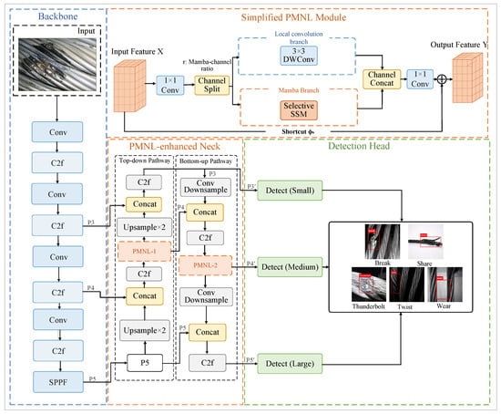
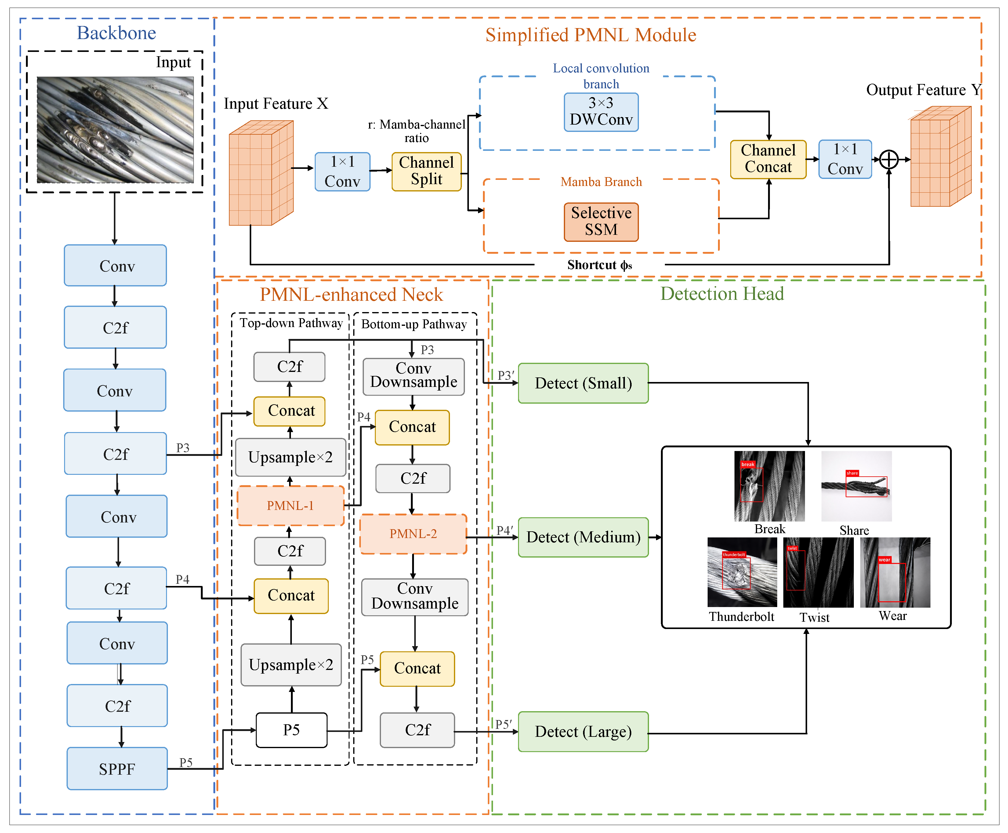
YOLOv8s-PMNL retains the YOLOv8s backbone and detection head and inserts PMNL at two neck fusion sites (Figure 1). The backbone extracts hierarchical features through convolution and C2f modules. During multi-scale fusion, PMNL combines local texture and boundary cues with partial-channel state-space context; the unchanged head performs classification and bounding-box regression.

Figure 1. Overall architecture of YOLOv8s with Partial Mamba Neck Lite (PMNL) modules incorporated at two neck fusion sites; the backbone and detection head are retained. The upper panel shows a simplified PMNL schematic; the detailed branch operations are shown in Figure 2.

2.2. Partial-Channel Local–Long-Range Co-Modeling

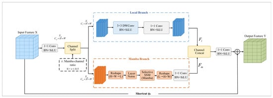
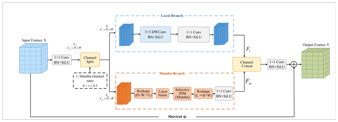
PMNL splits projected features between local convolution and Mamba branches (Figure 2). The branches combine spatial detail with sequence-based context without explicitly encoding orientation or aspect ratio; geometry-specific benefits are evaluated in Section 3.2.

Figure 2. Detailed structure of PMNL. The projected feature is split into a local branch with $C_l$ channels and a Mamba branch with $C_m$ channels. The local branch performs depthwise spatial processing followed by pointwise projection, whereas the Mamba branch applies sequence rearrangement, LayerNorm, selective state-space modeling, and output projection. The two branch outputs are concatenated and fused through a $1\times 1$ projection before residual addition through the shortcut mapping (${\varphi }_s$). All PMNLConv blocks consist of convolution, batch normalization, and SiLU activation.

Given an input feature map ($X\in {\mathbb{R}}^{C\times H\times W}$), a $1\times 1$ convolution first projects the input:

$$X_p={\varphi }_p\left(X\right),$$

(1)

where ${\varphi }_p$ denotes the channel projection and the projected feature ($X_p$) has $C_p$ channels. The feature is then split along the channel dimension into a local branch ($X_l$) and a Mamba branch ($X_m$):

$$[X_l,X_m]=\mathrm{Split}(X_p,r),$$

(2)

where r is the nominal Mamba-channel ratio, restricted to $0<r\le 0.5$ to retain an explicit local branch. The channel counts are

$$\begin{array}{cc}\hfill C_m& =\min \left(⌊{\displaystyle \frac{C_p}{2}}⌋,\max \left(16,⌊r{C}_p⌋\right)\right),\hfill \\ \hfill C_l& =C_p-C_m,\hfill \end{array}$$

(3)

Here, $C_m$ and $C_l$ are the Mamba and local channel counts. Integer allocation applies a nominal minimum of 16 channels, subject to a half-channel cap that preserves the local branch. The Full Mamba model evaluated below is a separate structural reference, not an $r=1$ member of PMNL.

2.3. Channel Allocation Strategy

The r ratio specifies the nominal proportion of projected channels assigned to the Mamba branch. We restrict $0<r\le 0.5$ so that an explicit local-convolution branch is retained at every PMNL site. Smaller values preserve more local-processing capacity and use fewer state-space channels; larger values allocate more capacity to long-range modeling at potentially higher computational and memory cost. Integer rounding and the minimum-channel and half-channel-cap rules in Equation (3) can make the realized layer-wise proportions differ slightly from the nominal ratio. We screen five ratios using observed strict-IoU validation accuracy and parameter count; the selection and its scope are detailed in Section 3.1.

The local branch applies a $3\times 3$ depthwise convolution followed by a $1\times 1$ pointwise projection. Both operations are implemented with the PMNL convolution block, consisting of convolution, batch normalization, and SiLU activation:

$$F_l={\varphi }_l^{1\times 1}\left({\varphi }_l^{\mathrm{dw}3\times 3}\left(X_l\right)\right),$$

(4)

where ${\varphi }_l^{\mathrm{dw}3\times 3}$ and ${\varphi }_l^{1\times 1}$ denote the depthwise and pointwise PMNL convolution blocks, respectively.

The Mamba branch rearranges $X_m$ into a spatial sequence of length $L=HW$, applies LayerNorm followed by selective state-space modeling, restores the spatial layout, and finally performs a $1\times 1$ output projection:

$$F_m={\varphi }_m^{1\times 1}\left\{{\mathcal{R}}^{-1}\left[\mathcal{M}\left(\mathrm{LN}\left[\mathcal{R}\left(X_m\right)\right]\right)\right]\right\},$$

(5)

where $\mathcal{R}$ and ${\mathcal{R}}^{-1}$ denote the spatial-to-sequence rearrangement and its inverse, respectively; LN denotes LayerNorm; and $\mathcal{M}$ denotes selective state-space modeling. The output projection (${\varphi }_m^{1\times 1}$) is implemented by a $1\times 1$ convolution followed by batch normalization and SiLU activation.

The branch outputs are concatenated and fused with a $1\times 1$ projection, followed by a residual shortcut:

$$Y={\varphi }_o\left[\mathrm{Concat}(F_l,F_m)\right]+{\varphi }_s\left(X\right),$$

(6)

Here, ${\varphi }_o$ is a $1\times 1$ PMNL convolution. When the input and output channel counts match, ${\varphi }_s$ is the identity; otherwise, it is a $1\times 1$ PMNL convolution. The r ratio is selected in Section 3.1.

The term “Lite” refers to the reduced allocation of state-space channels relative to the Full Mamba reference, rather than a claim of lower runtime than the original YOLOv8s baseline. In the reported YOLOv8s configuration, both PMNL sites have $C_{\mathrm{in}}=C_{\mathrm{out}}=C_p=256$ and use $r=0.25$, giving $C_m=64$ Mamba channels and $C_l=192$ local channels under Equation (3). The implementation uses mamba_ssm.Mamba with $d_{\mathrm{state}}=16$, $d_{\mathrm{conv}}=4$, and an expansion factor of 2. The Mamba input sequence is formed by flattening the spatial dimensions to $[B,HW,C_m]$, followed by LayerNorm and Mamba processing, and is then restored by the inverse transpose and reshape. The spatial sequence uses a single row-major order (width varying fastest), without additional reverse or multidirectional scans.

2.4. State-Space Modeling and TensorRT Deployment

The Mamba branch models spatial dependencies through selective state propagation. For the partial-channel feature ($X_m$), the spatial sequence is $S=\mathcal{R}\left(X_m\right)={\left\{s_t\right\}}_{t=1}^L$, where $L=HW$. Following the selective state-space formulation of Mamba [12], the state update is expressed as

$$h_t={\overline{A}}_t{h}_{t-1}+{\overline{B}}_t{s}_t,$$

(7)

where $s_t$ and $h_t$ denote the input feature and hidden state at position t, respectively. The input-dependent discretized ${\overline{A}}_t$ and ${\overline{B}}_t$ matrices govern state propagation and input injection, respectively.

The profiling results identify the retained Mamba route as a runtime bottleneck. The ablation and profiling results in Section 3.4 therefore motivate optimization of its selective scan paths.

The export-safe PyTorch graph is converted to Open Neural Network Exchange (ONNX) using two custom pmnl::PMNLSelectiveScan operators, implemented through a CUDA-backed TensorRT IPluginV3 plugin [22] for 32-bit floating-point (FP32) inference, preserving topology, trained weights, and state-transition semantics. In the reported deployment experiment, the runtime registered the creator PMNLSelectiveScan with version 4 and an empty namespace under TensorRT 10.4.0. ONNX serves only as an intermediate deployment representation; no independent ONNX Runtime accuracy benchmark is performed.

2.5. Datasets, Training Configuration, and Evaluation Metrics

The primary experiments use a locally reorganized export (DD.v1.yolov8) of the public wire-rope dataset dd, released by 4love on Roboflow Universe [23]. It contains five categories: Break, Share, Thunderbolt, Twist, and Wear. The original dataset class labels are retained throughout this study. The data were repartitioned into training, validation, and held-out test sets at approximately 70:15:15, followed by offline augmentation of the training set only. The final sets contain 5633, 1114, and 1116 images and 12,106, 2239, and 2464 defect instances, respectively.

Offline augmentation. The base training partition, before the additional local augmentation pass, contained 5203 images and 11028 bounding boxes. Class-targeted augmentation was performed with Albumentations on Windows before transfer to the RTX 4090 training server. This generation pass was limited to 150 eligible training images containing Share, Twist, or Wear. Images containing these classes were assigned four, three, or two candidate variants, respectively; for co-occurring target classes, the maximum applicable count was used. The saved parent–derivative mapping identifies 33 parents with four variants, 64 with three, and 53 with two, yielding 430 additional images and 1078 boxes. Retaining the base training files gives the reported total of 5633 images and 12,106 boxes. The existing validation and test files received no additional transformations from this offline pass.

Transformations and bounding-box handling. The offline transformations were considered in the order listed in Table 1. Bounding boxes and class labels were processed together in YOLO format. The visibility threshold was set to min_visibility = 0.35; boxes below this threshold were removed, together with their class labels. Each candidate received, at most, ten attempts in total and was skipped if all attempts retained no bounding boxes. Coordinates were written to six decimal places. Python seed 42 was specified in the generation script; the fixed augmented files, parent–derivative mapping, and image/annotation hashes form the saved record of this augmentation pass.

Table 1. Offline augmentation operations in execution order. The listed probabilities are configured for each generation attempt.

Operation	Parameters	p
Horizontal flip	HorizontalFlip	0.50
Affine transformation	Scale: 0.95–1.05; translation fraction: $-0.03$–0.03; rotation: $-5$–$5^{\circ }$; shear: $-2$–$2^{\circ }$	0.70
Brightness and contrast	brightness_limit = 0.12; contrast_limit = 0.12	0.50
HSV adjustment	Hue, saturation, and value shift limits: 4, 8, and 4	0.20
OneOf: blur	MotionBlur(blur_limit = 3); or GaussianBlur(blur_limit = (3,5))	0.15 (group)
OneOf: enhancement	CLAHE: clip limit 2.0, grid $8\times 8$; Sharpen: alpha 0.10–0.25, lightness 0.9–1.1; or GaussNoise(std_range = (0.02,0.06))	0.20 (group)

Note: Each activated OneOf group selects one listed member. The probability applies to the group; member p = 1.0 values do not mean that all members are applied. Configured probabilities are not measured frequencies among the 430 retained variants because attempts yielding no retained boxes are retried subject to the ten-attempt limit.

Online training settings. The six saved training configurations for the principal YOLOv8s–PMNL comparison, covering seeds 0, 42, and 3407 for both models, specify identical online augmentation arguments. HSV gains were set to 0.01, 0.4, and 0.2 for hue, saturation, and value, respectively. The geometric arguments were degrees = 5, translate = 0.03, scale = 0.1, and shear = 2. Horizontal and vertical flip probabilities were configured as 0.5 and 0, respectively. Mosaic was configured with mosaic = 0.2 and close_mosaic = 15. The MixUp, CutMix, copy–paste, perspective, BGR-reversal, and multi-scale arguments were zero, and rectangular batching was disabled. These are the saved online augmentation settings for training on the fixed offline dataset.

Additional evaluation uses GC10-DET [24], with 2294 images and 3564 instances after YOLO-format conversion. The seed-42 split contains 1606 training, 344 validation, and 344 test images. Both models were retrained with seeds 42, 0, and 3407 using matched AdamW settings (initial learning rate of 0.001, weight decay of 0.0005); identical online augmentation; and, at most, 120 FP32 epochs. The cable-experiment recipe was retained without a GC10-specific hyperparameter sweep; checkpoints were selected by validation (${\mathrm{mAP}}_{0.50:0.95}$). Evaluation uses unfused exponential moving average (EMA) weights in FP32, imgsz = 800, and rectangular batches.

The validation and test files were kept unchanged during the additional local offline augmentation pass. Model selection, channel-ratio screening, and parameter tuning use only training and validation data. Testing begins only after the model configuration and training protocol are fixed. The principal YOLOv8s–PMNL comparison reports validation mean and sample standard deviation over three independent runs (seeds 0, 42, and 3407), with held-out testing using each model’s fixed seed-42 checkpoint.

For the framework-level comparison, all final checkpoints were re-evaluated on the same validation split under matched evaluation settings: 1114 images, imgsz = 800 with rectangular batching, batch size of 8, confidence threshold of 0.001, non-maximum suppression (NMS) with an intersection-over-union (IoU) threshold of 0.70, and FP32 precision. YOLOv5s used its native YOLOv5 evaluator, whereas the remaining models used their compatible Ultralytics implementations; the test set was not used. Because several detectors retain their official training pipelines, the training recipes are not identical. We therefore treat this as a reference comparison under matched evaluation conditions, not as a strictly controlled training-level ablation.

Experiments were conducted on an NVIDIA GeForce RTX 4090 workstation. Table 2 summarizes the main detector-training configuration; series-specific evaluation conditions are listed in Table 3.

Table 2. Main detector-training configuration. GPU denotes graphics processing unit, OS denotes operating system, AMP denotes automatic mixed precision, and LR denotes learning rate.

Item	Setting	Item	Setting
GPU	RTX 4090	Input size	$800\times 800$
OS	Ubuntu 24.04	Max. epochs	120
Python	3.12.3	Batch size	20
PyTorch	2.5.1+cu121	Optimizer	AdamW
CUDA	12.1	Initial LR	0.001
Ultralytics	8.4.43	Final LR factor	0.01
AMP	False	Weight decay	0.0005
Pretrained	True	Workers	4
Seeds	0, 42, 3407	Patience	40
Split	Train/Val/Test	Ratio	70/15/15

Note: The split ratio refers to the partition before the additional training-set augmentation. GPU denotes graphics processing unit, OS denotes operating system, AMP denotes automatic mixed precision, and LR denotes learning rate.

Table 3. Overview of the experimental series and their comparison scopes. Comparisons are interpreted within the corresponding checkpoint series and evaluation or timing protocol.

Series	Checkpoints and Purpose	Evaluation/Execution	Valid Comparison
Ratio and site screening	Reduced 40-epoch protocol; ratio screening uses seed 42	Main-data validation; ratio and site variants	Design screening within the reduced training budget
Structural comparison	Independent 120-epoch series; seeds 42, 0, and 3407; Matched Conv, Partial PMNL, and Full Mamba	Common split and evaluation within the series; seed-42 native timing uses FP32, TensorFloat-32 (TF32) off, batch 1, unfused models	Structural effects within this series; separate from baseline repeatability
Baseline repeatability	Three-seed validation; fixed seed-42 checkpoints for held-out testing	Main-data validation (1114 images) and test (1116 images)	YOLOv8s versus PMNL; validation means and single-seed test scores reported separately
Framework comparison	Detector-specific final checkpoints; training recipes differ	Validation: FP32, batch 8, confidence 0.001, NMS IoU 0.70; YOLOv5 native/compatible Ultralytics evaluators. Native timing: FP32, batch 1	Detector comparison under matched evaluation settings; not an identical-training-recipe ablation
GC10-DET held-out testing	Independent retraining; seeds 42, 0, and 3407; fixed split seed 42	Held-out test on 344 images; mean and sample standard deviation	Second-dataset performance after retraining, not zero-shot transfer
Original deployment	Fixed seed-42 PMNL checkpoint for backend consistency; original engines for core-inference timing	Consistency: 1114 images, batch 1, TensorRT FP32, unchanged preprocessing, NMS and metrics. Timing: forward/TensorRT execution only	Backend fidelity within a fixed configuration; The original-engine benchmark reports core latency
Matched partial–full deployment	Seed-42 structural-series checkpoints; independently rebuilt engines	TensorRT 10.4, FP32, TF32 off, builder level 1, same scan plugin, batch 1; validation on 1114 images	Partial versus full under the same deployment protocol; independent of the original-engine benchmark
Software-path end-to-end	Same matched partial–full engines and plugin	RTX 4090, TensorRT 10.4, FP32, batch 1; 100 warm-ups; 5 groups × 1000 iterations; all 1114 images	Host-specific end-to-end software-path latency; separate from core-inference timing

Note: The framework and structural validation series use imgsz = 800 with rectangular batching and batch sizes 8 and 40, respectively, in their Ultralytics evaluators. The structural series uses the archived Ultralytics 8.4.22 implementation and unfused models. Deployment evaluation and core-inference timing use fixed 800 × 800 input with a batch size of 1. Core-inference timing excludes preprocessing, NMS and postprocessing; it is not end-to-end system latency. The standalone scan benchmark uses FP32 tensors with dimensions of 1 × 128 × 2500 and TF32 disabled and measures operator execution separately. Geometry, category and corruption analyses characterize performance on the validation set; qualitative examples use the held-out test set and are not estimates of subgroup success rates. Statistics across training seeds and across timing repeats quantify different sources of variation.

Detection performance is evaluated using precision (P), recall (R), and mean average precision (mAP), reported as ${\mathrm{mAP}}_{0.50}$, ${\mathrm{mAP}}_{0.75}$, ${\mathrm{mAP}}_{0.90}$, and ${\mathrm{mAP}}_{0.50:0.95}$. The stricter thresholds of 0.75 and 0.90 assess localization accuracy, while ${\mathrm{mAP}}_{0.50:0.95}$ summarizes performance across IoU thresholds from 0.50 to 0.95 in increments of 0.05. Parameter count (Params), latency, and throughput in frames per second (FPS) characterize model size and inference efficiency.

The experimental series in Table 3 address distinct questions. Accuracy and latency comparisons remain within each checkpoint series and protocol; cross-series results do not define a common accuracy–speed operating point.

3. Results

3.1. Channel Allocation and Repeatability

Channel allocation is screened over five ratios using seed 42 and 40 epochs (Table 4). Optimization and augmentation remain fixed; only the branch allocation varies. Final accuracy and repeatability are evaluated separately under the main protocol.

Table 4. Mamba-channel ratio screening under the controlled 40-epoch protocol with seed 42. The r ratio denotes the nominal proportion of projected channels assigned to the Mamba branch; mAP values are percentages.

r	Params	mAP (%)
	(M)	0.50	0.75	0.90	0.50:0.95
0.1250	11.530	93.334	60.274	10.239	57.915
0.2500 a	11.554	93.748	62.032	12.213	58.399
0.3750	11.613	93.775	60.317	11.602	57.961
0.4375	11.654	93.933	61.230	11.428	57.972
0.5000	11.705	93.746	62.275	11.788	58.781

Note: Bold values indicate the highest mAP in each corresponding IoU metric column. ^a Selected for subsequent PMNL experiments.

In the 40-epoch screen with seed 42 (Table 4), $r=0.25$ achieves the highest observed ${\mathrm{mAP}}_{0.90}$ (12.213%), exceeding $r=0.50$ by 0.425 percentage points with 0.150 M fewer parameters. We retain $r=0.25$ to prioritize strict-IoU localization and model size, accepting lower aggregate ${\mathrm{mAP}}_{0.50:0.95}$ (58.399% versus 58.781%; a decrease of 0.382 percentage points). The reported evaluation does not compare TensorRT latency, memory, or throughput across the five ratios; Full Mamba is a separate structural reference, not another PMNL ratio setting. Thus, multi-seed stability of the ratio ranking and a deployment-optimal ratio remain unverified.

An independent 120-epoch structural series compares parameter-matched convolution, Partial PMNL, and Full Mamba using seeds 42, 0, and 3407. The split, optimization, and evaluation settings are identical across structures, and seed selection is independent of the measured outcome. All checkpoints are loaded and evaluated in FP32. The seed-42 Partial PMNL and Matched Conv checkpoints were stored in FP16, whereas the corresponding Full Mamba checkpoint was stored in FP32. We interpret scores within this series separately from the 40-epoch screening and baseline repeatability experiments.

Controlled structural references. The three variants occupy the same two neck sites (zero-based indices 13 and 20), each with 256-channel input/output interfaces. Matched Conv replaces the state-space branch with local convolutions; Partial PMNL retains 192 local channels and 64 Mamba channels. Full Mamba uses a separate FullChannelMamba block with all 256 projected channels assigned to Mamba and the parallel local branch and concatenation removed. Its sequence is $1\times 1$ pre-projection, flattening to $[B,HW,256]$, LayerNorm, mamba_ssm.Mamba ($d_{\mathrm{model}}=256$, $d_{\mathrm{state}}=16$, $d_{\mathrm{conv}}=4$, expansion factor 2), spatial restoration, $1\times 1$ output projection, $1\times 1$ fusion, and identity residual addition. All three projections use Conv–BN–SiLU, and the surrounding detector architecture is unchanged. This is a separately constructed reference, not the $r=1$ setting of PMNL. The Full Mamba detector has 12.4104 M parameters; Matched Conv and Partial PMNL have 11.5543 M and 11.5544 M, respectively, differing by less than 0.001%.

Partial PMNL improves aggregate mAP over matched convolution by 2.515 percentage points despite a parameter difference below 0.001% (Table 5). Gains at IoU values of 0.75 and 0.90 are 4.038 and 4.419 points, consistent with an effect beyond parameter growth. Full Mamba remains most accurate; relative to Full Mamba, Partial PMNL is 1.757 percentage points lower in aggregate mAP and uses 6.90% fewer parameters.

Table 5. Three-seed controlled structural comparison under the 120-epoch training protocol. Accuracy values are mean ± sample standard deviation (%) over seeds 42, 0, and 3407.

Model	${\mathbf{mAP}}_{0.50}$	${\mathbf{mAP}}_{0.75}$	${\mathbf{mAP}}_{0.90}$	${\mathbf{mAP}}_{0.50:0.95}$	Params (M)
Matched Conv	$95.838\pm 0.101$	$74.591\pm 0.159$	$32.347\pm 1.569$	$68.590\pm 0.344$	11.5543
Partial PMNL	$96.128\pm 0.122$	$78.629\pm 0.827$	$36.766\pm 1.616$	$71.105\pm 0.528$	11.5544
Full Mamba	$\mathbf{96.386}\pm \mathbf{0.055}$	$\mathbf{81.515}\pm \mathbf{1.084}$	$\mathbf{37.658}\pm \mathbf{1.149}$	$\mathbf{72.863}\pm \mathbf{0.552}$	12.4104

Note: Bold values indicate the highest mean performance in each corresponding mAP metric column.

Native runtime is measured on the RTX 4090 using fixed seed-42 checkpoints, FP32, TF32 disabled, unfused models, a batch size of 1, $800\times 800$ input, and order-balanced CUDA-event timing. Matched Conv, Partial PMNL, and Full Mamba require $6.675\pm 0.018$, $7.908\pm 0.107$, and $7.470\pm 0.031$ ms, respectively (149.82, 126.45, and 133.87 FPS), with peak allocated memory of 111.24, 119.36, and 122.15 MiB. Partial PMNL uses 2.28% less peak memory than Full Mamba but is 5.87% slower. TensorRT efficiency is assessed separately in Section 3.5.

Across these measured points, no structure dominates every criterion. Matched Conv has the lowest native latency and parameter count but lower accuracy; Full Mamba forms the accuracy-oriented boundary, while Partial PMNL occupies an intermediate accuracy–resource point. TensorRT changes this ordering: Partial PMNL has lower core latency, engine size, device memory, and software-path end-to-end mean latency than Full Mamba. This reading is protocol-specific; the proposed ratio was not obtained by solving a formal multi-objective optimization problem.

Table 6 reports the independent YOLOv8s–PMNL baseline series: three-seed validation and held-out testing with fixed seed-42 checkpoints after architecture and protocol selection.

Table 6. Repeated validation and held-out test results (%).

Model	${\mathbf{mAP}}_{0.50}$	${\mathbf{mAP}}_{0.75}$	${\mathbf{mAP}}_{0.90}$	${\mathbf{mAP}}_{0.50:0.95}$
Validation set: three seeds, mean ± sample standard deviation
YOLOv8s	$95.450\pm 0.313$	$72.205\pm 0.582$	$26.687\pm 1.107$	$65.625\pm 0.344$
YOLOv8s-PMNL	$\mathbf{95.758}\pm \mathbf{0.252}$	$\mathbf{79.024}\pm \mathbf{0.201}$	$\mathbf{32.866}\pm \mathbf{0.407}$	$\mathbf{70.191}\pm \mathbf{0.215}$
Held-out test set: fixed seed-42 checkpoints
YOLOv8s	94.814	65.191	17.880	61.376
YOLOv8s-PMNL	95.866	78.866	31.202	69.636

Note: Bold values indicate the higher result for each metric within the corresponding validation or held-out test group. Italic text identifies the evaluation groups.

PMNL improves validation ${\mathrm{mAP}}_{0.50:0.95}$ by 4.566 percentage points, with gains of 6.819 and 6.179 points at IoU values of 0.75 and 0.90, respectively. Its sample standard deviation is lower across all four metrics. On the 1116 held-out images, aggregate mAP reaches 69.636% and exceeds YOLOv8s by 8.261 points. Gains at IoU values of 0.50, 0.75, and 0.90 are 1.052, 13.674, and 13.322 points, respectively. These gains are calculated from unrounded values. The larger strict-IoU improvements support more accurate localization.

3.2. Geometry, Robustness, and Qualitative Analysis

Performance is further analyzed with respect to target geometry, defect category, and image degradation. For each ground-truth box with normalized width (w) and height (h), the normalized area (A) and aspect ratio ($\rho$) are defined as

$$A=wh,\rho ={\displaystyle \frac{\max (w,h)}{\min (w,h)}}.$$

(8)

Following the COCO area convention [25], the ${32}^2$ and ${96}^2$ thresholds are normalized to the $800\times 800$ input resolution, giving Small ($A<0.0016$), Medium ($0.0016\le A<0.0144$), and Large ($A\ge 0.0144$) groups. Morphology thresholds are obtained from the 75th and 90th percentiles of the training-set aspect-ratio distribution: Regular ($\rho <2.192$), Elongated ($2.192\le \rho <3.620$), and Very-Elongated ($\rho \ge 3.620$). All thresholds are fixed before validation.

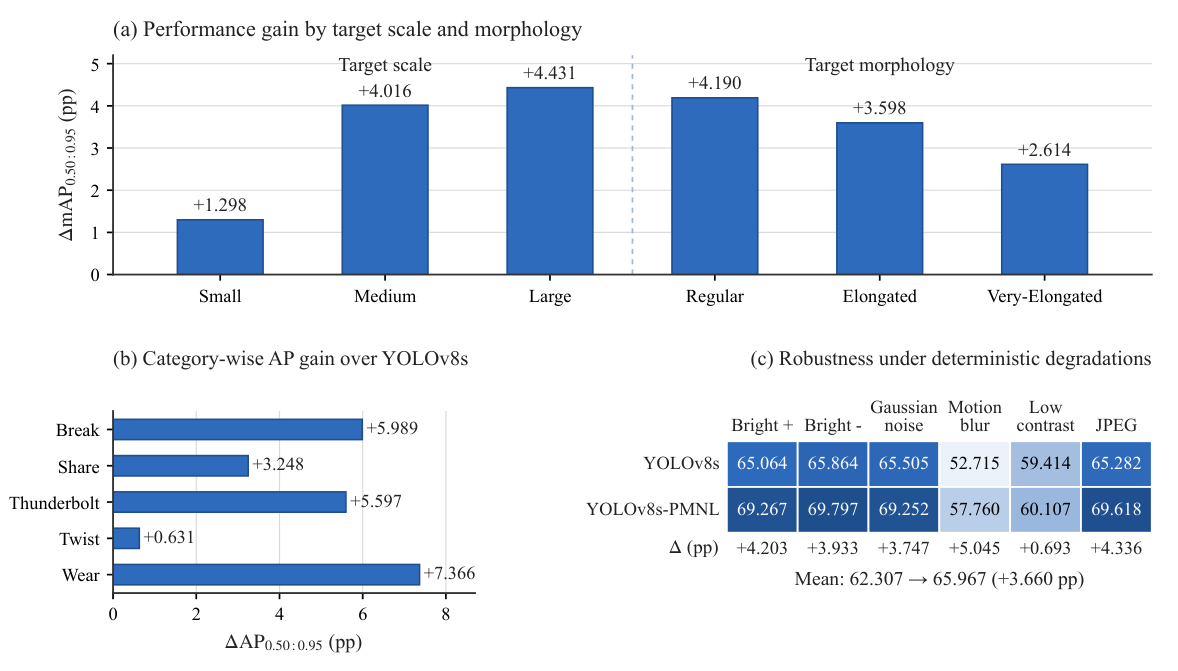
Figure 3a reports aggregate mAP gains of 1.298, 4.016, and 4.431 percentage points for Small, Medium, and Large targets. The corresponding gains for Regular, Elongated, and Very-Elongated targets are 4.190, 3.598, and 2.614 points. Gains persist for elongated defects but decline with aspect ratio. Because scale and morphology are evaluated separately and may covary with category and frequency, these results do not isolate a shape-specific mechanism. Category-wise gains are 5.989, 3.248, 5.597, 0.631, and 7.366 points for Break, Share, Thunderbolt, Twist, and Wear, respectively (Figure 3b).

Figure 3. Comparison of YOLOv8s-PMNL with YOLOv8s: (a) ${\mathrm{mAP}}_{0.50:0.95}$ gains across target scales and morphologies, (b) category-wise average precision (AP)_0.50:0.95 gains, and (c) robustness under deterministic image degradations. Gains are reported in percentage points.

Robustness is evaluated with an author-defined deterministic corruption robustness protocol (RCP-v1): brightness factors of 1.2 and 0.8, Gaussian noise ($\sigma =10$), 7-pixel motion blur at ${45}^{\circ }$, low contrast ($\alpha =0.70$), and Joint Photographic Experts Group (JPEG) quality of 50. Both models use identical corrupted validation images generated with seed 20260829. PMNL yields a higher measured mAP under all six conditions (Figure 3c), increasing mean aggregate mAP from 62.307% to 65.967%. Gains range from 0.693 points under low contrast to 5.045 under motion blur. Higher accuracy on corrupted images alone does not establish a smaller degradation from clean accuracy, and global contrast reduction does not constitute texture-stratified evaluation.

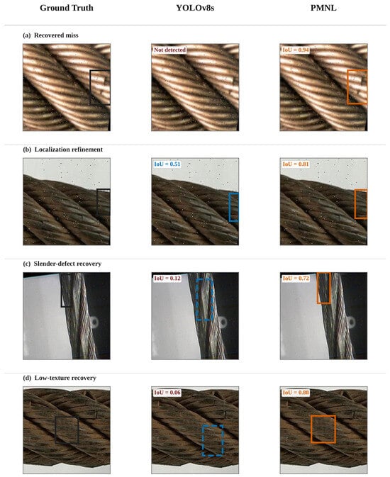
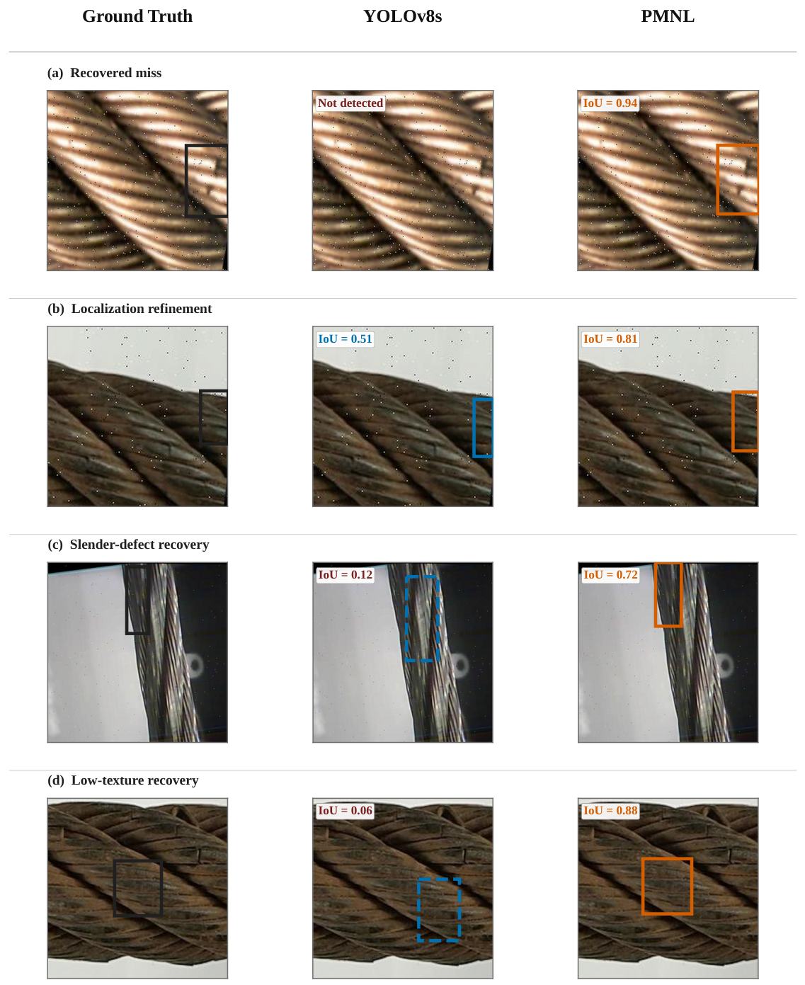
Qualitative analysis compares the fixed YOLOv8s and PMNL checkpoints on all 1116 held-out test images. Inference uses a confidence of 0.001 and NMS IoU of 0.70; visualization retains post-NMS predictions with confidence $\ge 0.25$. Each ground-truth instance is matched to the highest-IoU same-class prediction, with zero IoU assigned to unmatched targets. A hit requires IoU $\ge 0.50$. Localization refinement requires a hit from both models, PMNL IoU $\ge 0.75$, and an IoU gain of at least 0.15.

The selected examples in Figure 4 improve matched IoU from 0 to 0.944 (recovered miss), 0.506 to 0.814 (refined localization), 0.116 to 0.723 (slender defect), and 0.061 to 0.881 (low-texture defect). They do not establish subgroup success rates or a population-level advantage for low-texture defects.

Figure 4. Representative localization behaviors on the held-out test set. Columns show the ground truth, YOLOv8s prediction, and PMNL prediction, respectively. Black solid boxes denote ground truth, blue boxes denote YOLOv8s predictions, and orange solid boxes denote PMNL predictions. The dashed blue boxes in (c,d) mark low-overlap YOLOv8s predictions (IoU $<0.50$). The four examples illustrate (a) missed-defect recovery, (b) localization refinement, (c) slender-defect recovery, and (d) low-texture recovery. The displayed IoU values denote the highest overlap with a retained same-class prediction for the target ground-truth instance under the fixed qualitative-analysis rule described in the text.

Paired failure analysis. We analyzed the saved predictions of the fixed seed-42 YOLOv8s and PMNL checkpoints on all 1116 held-out test images and 2464 ground-truth (GT) instances. The main diagnostic operating point retains post-NMS predictions with confidence $\ge 0.25$, using NMS IoU 0.70 and matching IoU $\ge 0.50$. Same-class GT–prediction pairs are sorted by decreasing IoU and accepted greedily only when neither instance has already been assigned; ties are resolved by GT and prediction row order. Each GT is classified as detected by both models, detected only by YOLOv8s (PMNL regression), detected only by PMNL (PMNL recovery), or unmatched by both. Regression and recovery percentages use all GT instances in the corresponding group as the denominator. Scale groups use the normalized-area thresholds defined above. These population counts use one-to-one matching; the preceding qualitative examples retain their displayed maximum-overlap IoUs.

Background-texture grouping. For each GT, we measured the surrounding background after bilinear resizing to a longest edge of 800 pixels, preserving aspect ratio without padding. Grayscale intensities are normalized to $[0,1]$. Within the GT rectangle enlarged by a factor of 1.5 about its center and clipped to the image, all annotated GT regions are excluded. The score is $T=\mathrm{mean}(G_x^2+G_y^2)$, where $G_x$ and $G_y$ are $3\times 3$ Sobel responses divided by 8. Only gradient centers whose entire kernel support lies in valid background are retained. Regions with fewer than 64 valid centers are labeled Unassigned. Low, Medium, and High groups are defined by the 33rd and 67th percentiles of 11,986 valid GT neighborhoods from the existing 5633-image training partition, including its offline derivatives: $q_{33}\approx 1.547148\times {10}^{-3}$ and $q_{67}\approx 3.249645\times {10}^{-3}$. Low corresponds to $T\le q_{33}$, Medium to $q_{33}<T\le q_{67}$, and High to $T>q_{67}$. These training-derived thresholds are applied to the test set. This background measure differs from the defect-crop grayscale variation used to select the low-texture example in Figure 4d.

Failure distribution. At the main operating point, 2122 GT instances are detected by both models, 73 regress from YOLOv8s to PMNL, 54 are recovered by PMNL, and 215 remain unmatched by both models (Table 7). Medium targets account for 62 of the 73 regressions (84.93%) and have the highest scale-specific regression rate (4.18%). All 62 belong to Break or Wear. Break contributes 46 regressions (4.27% of its GT instances), and Wear contributes 25 (3.03%); together, these categories account for 71 of the 73 regressions (97.26%).

Table 7. Paired detection outcomes on the held-out test set at confidence $\ge 0.25$ and matching IoU $\ge 0.50$.

Group	GT N	Both Detected	Regression n (%)	Recovery n (%)	Both Unmatched	PMNL Unmatched n (%)
Overall	2464	2122	73 (2.96)	54 (2.19)	215	288 (11.69)
Target scale
Small	90	31	2 (2.22)	3 (3.33)	54	56 (62.22)
Medium	1483	1244	62 (4.18)	41 (2.76)	136	198 (13.35)
Large	891	847	9 (1.01)	10 (1.12)	25	34 (3.82)
Defect category
Break	1078	841	46 (4.27)	34 (3.15)	157	203 (18.83)
Share	101	100	0 (0.00)	1 (0.99)	0	0 (0.00)
Thunderbolt	252	243	2 (0.79)	0 (0.00)	7	9 (3.57)
Twist	209	208	0 (0.00)	0 (0.00)	1	1 (0.48)
Wear	824	730	25 (3.03)	19 (2.31)	50	75 (9.10)
Background texture
Low	776	698	25 (3.22)	15 (1.93)	38	63 (8.12)
Medium	803	715	20 (2.49)	24 (2.99)	44	64 (7.97)
High	863	701	28 (3.24)	15 (1.74)	119	147 (17.03)
Unassigned	22	8	0 (0.00)	0 (0.00)	14	14 (63.64)

Note: Regression means YOLOv8s-only detection; recovery means PMNL-only detection. Both detected, regression, recovery, and both unmatched sum to GT N. PMNL unmatched equals regression plus both unmatched. All percentages use group-specific GT N. The scale, category, and texture sections are overlapping descriptions of the same test instances. Unassigned denotes insufficient valid background.

Small targets have a high PMNL unmatched rate of 56/90 (62.22%), including 54 targets unmatched by both models. Only two small targets regress, and three are recovered, identifying small-target detection as predominantly a shared difficulty at this operating point. Among the assigned background-texture groups, High has a larger PMNL unmatched rate (17.03%) than Low (8.12%) or Medium (7.97%). Its regression rate is 3.24%, however, which is close to 3.22% for Low. Within medium targets, the regression rates are 4.09% for High and 4.76% for Low. These are descriptive associations across groups with different category and scale composition rather than evidence of an independent texture-induced regression mechanism.

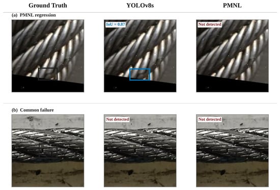
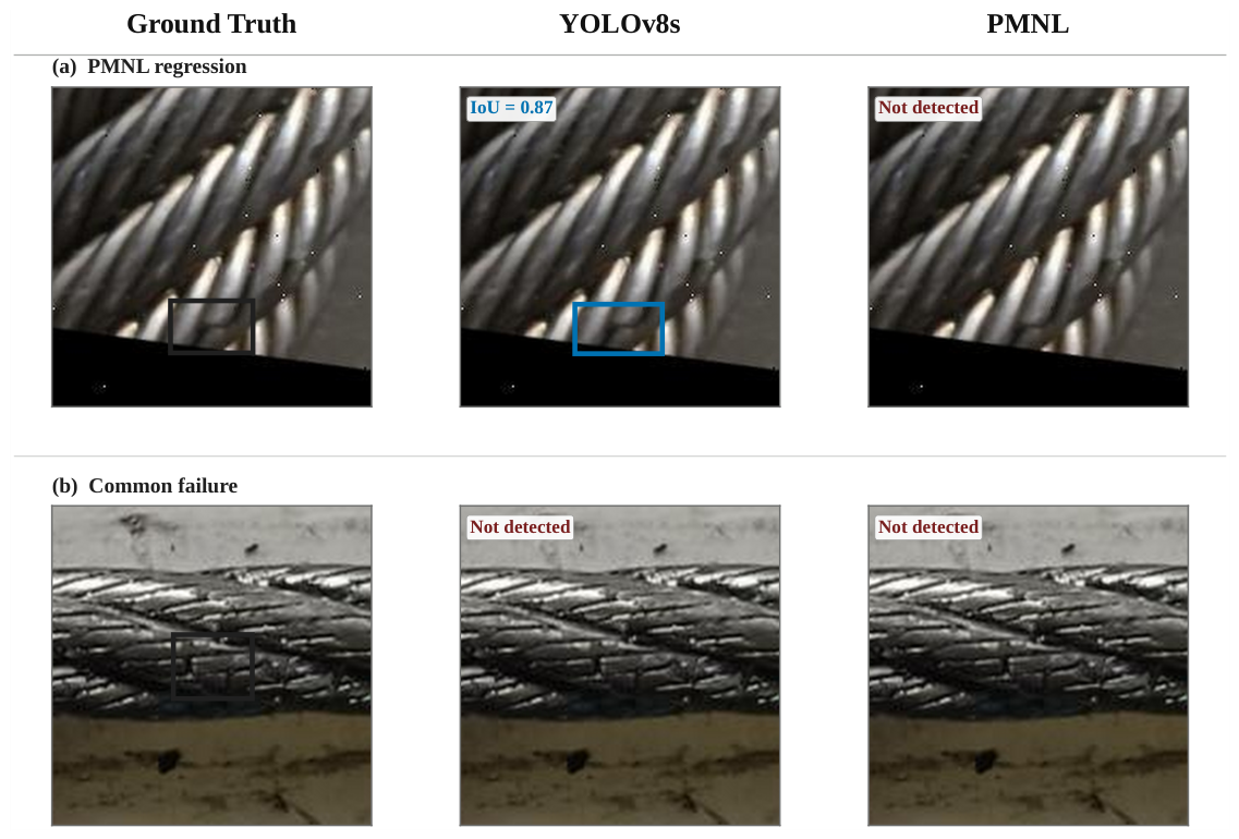
Figure 5a is a medium-sized Break regression in the High background-texture group, whereas Figure 5b is a small Break target in the same texture group that remains unmatched by both models. Thus, the examples correspond to distinct outcomes in the full-test-set statistics.

Figure 5. Representative failure cases on the held-out test set: (a) a medium-sized Break target in the high-background-texture group, detected by YOLOv8s at an IoU of 0.870 but unmatched by PMNL; (b) a small Break target in the high-background-texture group, unmatched by both models. The background-texture groups use the quantitative definition in the text. Black solid boxes denote ground truth, and the blue solid box denotes the YOLOv8s prediction in (a). No PMNL prediction box is shown; “Not detected” indicates that no prediction is retained for the target. Both cases are linked to the population statistics in Table 7.

Operating-point sensitivity. At a confidence of 0.25 and matching IoU of 0.50, recall is 89.083% for YOLOv8s and 88.312% for PMNL, while false positives decrease from 297 to 262 (0.266 to 0.235 per image). At a matching IoU of 0.50, confidence 0.10 gives 2249 versus 2223 matched GT instances, and confidence of 0.50 gives 2083 versus 2095, respectively. At a confidence of 0.25 and matching IoU of 0.90, PMNL matches 380 GT instances versus 321 for YOLOv8s; unmatched targets at this threshold do not meet the strict localization requirement and are not all complete detection misses. These counts describe fixed operating points and complement the reported AP evaluation.

3.3. Comparative Evaluation

YOLOv8s-PMNL is compared with representative convolutional, Transformer-based, and state-space detectors, including YOLOv5s [26], YOLOv8s [8], YOLOv10s [27], YOLO26s [28], RT-DETR-L [29], and Mamba-YOLO-T and Mamba-YOLO-B [18]. Final checkpoints are re-evaluated under the framework-level protocol in Section 2.5. Mamba-YOLO uses its official pipeline with the same dataset, $800\times 800$ input, a maximum of 120 epochs, seed 42, four workers, and early-stopping patience of 40 epochs. Batch sizes are 20 for Mamba-YOLO-T and 12 for Mamba-YOLO-B owing to GPU-memory constraints. Its use of SGD and automatic mixed precision means that training recipes differ across detectors despite matched final evaluation.

CSAMamba-YOLOv8 and CBH-YOLO are discussed as related work but are not included in this reference comparison because compatible training implementations and directly reproducible configurations were not established for this study.

Under the framework-level validation protocol, PMNL records the highest aggregate and strict-IoU mAP among the evaluated detectors (Table 8). Its aggregate mAP exceeds YOLOv8s by 6.821 percentage points, with gains of 9.642 and 10.136 points at IoU values of 0.75 and 0.90. YOLOv5s is fastest and has the highest ${\mathrm{mAP}}_{0.50}$; Mamba-YOLO-T has the fewest parameters. These rankings are conditional on the reported evaluation protocol and should not be interpreted as evidence of universal superiority across training recipes or hardware platforms.

Table 8. Reference comparison of accuracy and efficiency for representative detectors under the framework-level validation protocol.

Model	${\mathbf{mAP}}_{0.50}$	${\mathbf{mAP}}_{0.75}$	${\mathbf{mAP}}_{0.90}$	${\mathbf{mAP}}_{0.50:0.95}$	Params (M)	Latency (ms)	FPS
YOLOv5s	96.030	70.503	25.558	65.299	7.033	$\mathbf{5.660}\pm \mathbf{0.098}$	176.68
YOLOv8s	94.935	69.321	22.009	63.441	11.138	$8.332\pm 0.338$	120.02
YOLOv10s	95.018	70.062	28.358	64.823	8.070	$9.158\pm 0.868$	109.19
YOLO26s	95.187	70.450	30.203	65.519	9.952	$10.496\pm 0.574$	95.28
RT-DETR-L	95.851	73.109	29.074	66.862	32.816	$39.699\pm 0.487$	25.19
Mamba-YOLO-T	94.049	68.659	25.741	63.868	5.986	$6.572\pm 0.251$	152.16
Mamba-YOLO-B	95.332	74.353	29.156	67.149	21.799	$13.792\pm 0.130$	72.51
YOLOv8s-PMNL	95.476	78.963	32.145	70.262	11.554	$11.321\pm 0.988$	88.33

Note: mAP values (%) use the framework-level validation protocol in Section 2.5; the test set is not used. Parameter counts refer to unfused networks. Latency and FPS use native-framework inference on an RTX 4090 with 800 × 800 input, a batch size of 1, and FP32 precision. Training recipes and evaluator implementations differ across detectors; these results are reference comparisons, not a strictly controlled performance ranking (Section 3.3). The timing scope differs from the TensorRT core-inference benchmark reported later in the deployment evaluation. Best values in each column are bold.

Relative to Mamba-YOLO-T, PMNL gains 6.394 aggregate points but is larger and slower; relative to Mamba-YOLO-B, it gains 3.113 points with 47.00% fewer parameters and 17.92% lower native latency. These detector-level results are distinct from the controlled partial–full structural comparison. Relative to YOLOv8s, PMNL increases parameters by 3.74% but native latency by 35.88%, motivating component profiling.

On GC10-DET, mean ${\mathrm{mAP}}_{0.50:0.95}$ improves by 0.687 percentage points, whereas ${\mathrm{mAP}}_{0.90}$ decreases by 0.383 points (Table 9). Class ${\mathrm{AP}}_{0.50:0.95}$ improves in seven categories but decreases by 1.851 points for crease and 1.500 points for oil_spot. Post hoc diagnostics use the original class-consistent one-to-one AP matching at a confidence of 0.001. Pooling three runs on the same 547 test objects, matched counts increase from 1366 to 1405 at an IoU of 0.50 but decrease from 74 to 65 at an IoU of 0.90, with 22 shared, 52 baseline-only, and 43 PMNL-only strict matches. All 52 regressions remain matched by both models at an IoU of 0.50; PMNL’s best same-class IoUs range from 0.656 to 0.899. These observations identify a strict bounding-box alignment shortfall alongside the category-dependent aggregate gains.

Table 9. Three-seed held-out test results on GC10-DET (%).

Metric	YOLOv8s	PMNL
${\mathrm{mAP}}_{0.50}$	$58.392\pm 1.889$	$\mathbf{59.628}\pm \mathbf{1.839}$
${\mathrm{mAP}}_{0.75}$	$23.603\pm 1.558$	$\mathbf{24.051}\pm \mathbf{0.955}$
${\mathrm{mAP}}_{0.90}$	$\mathbf{1.598}\pm \mathbf{0.479}$	$1.215\pm 0.285$
${\mathrm{mAP}}_{0.50:0.95}$	$27.813\pm 1.352$	$\mathbf{28.500}\pm \mathbf{0.695}$

Note: Mean ± sample standard deviation over seeds 42, 0, and 3407. Best mean per metric is bold.

3.4. Structural Contribution and Runtime Bottleneck

Four variants are evaluated under the 40-epoch screening protocol: both Mamba paths retained, front path removed, rear path removed, and both paths removed. Ablations disable the state-space paths while retaining the remaining local-processing and projection/fusion topology as closely as possible.

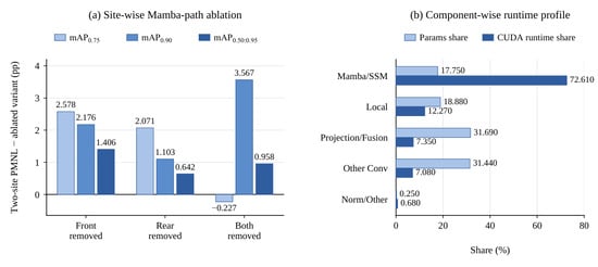
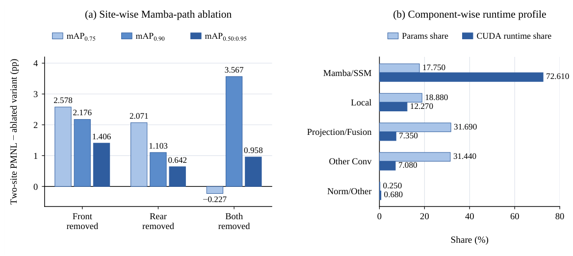
Among the site-ablation variants, the complete model achieves the highest aggregate mAP (58.399%) and ${\mathrm{mAP}}_{0.90}$ (12.213%). Front- and rear-path removal reduce aggregate mAP by 1.406 and 0.642 percentage points, respectively (Figure 6a); their decreases at an IoU of 0.75/0.90 are 2.578/2.176 and 2.071/1.103 points. Removing both paths reduces aggregate mAP by 0.958 points and ${\mathrm{mAP}}_{0.90}$ by 3.567 points but increases ${\mathrm{mAP}}_{0.75}$ by 0.227 points. Effects are therefore non-additive. These results favor retaining both sites within the evaluated budget, without establishing statistical significance.

Figure 6. Structural ablation and runtime profiling of PMNL. (a) Performance differences between the complete two-site PMNL and the front-, rear-, and both-site Mamba-path removal variants under the matched 40-epoch protocol. The difference is defined as $\Delta \mathrm{mAP}={\mathrm{mAP}}_{\mathrm{two}\text{-}\mathrm{site}}-{\mathrm{mAP}}_{\mathrm{ablated}}$, in percentage points: positive values indicate degradation after removal, whereas negative values indicate a slight improvement. (b) Parameter shares and diagnostic CUDA timing shares, normalized separately within the two PMNL modules. For Norm/Other, the parameter bar denotes separately categorized normalization weights, and the timing bar denotes recorded shortcut time.

Figure 6b compares parameter and diagnostic timing shares within the two PMNL modules. The Mamba/SSM group contains 0.073984M of their 0.416896M parameters (17.75%) and accounts for 2.2397 ms of 3.0846 ms of summed direct-child CUDA timings (72.61%). This group includes LayerNorm, Mamba, and its output projection; the timing share describes the grouped route rather than Scan alone or whole-network wall-clock latency. Parameter count measures stored weights; the Mamba branch additionally performs state propagation over the spatial sequence ($L=2500$ at each profiled site), so its parameter share does not predict its execution share. The imbalance identifies the retained Mamba route as an execution bottleneck, motivating its CUDA-backed TensorRT implementation in Section 3.5.

3.5. Numerically Consistent Selective Scan and TensorRT Evaluation

Backend fidelity is evaluated with a fixed seed-42 PMNL checkpoint on all 1114 validation images, using $1\times 3\times 800\times 800$ input; confidence of 0.001; NMS IoU of 0.70; and, at most, 300 detections per image. Preprocessing, NMS, and metrics remain unchanged; the test set is excluded. Native PyTorch, export-safe PyTorch, and TensorRT FP32 give identical reported mAP values: 94.7969%, 72.9571%, 26.9051%, and 66.3479% at IoU values of 0.50, 0.75, 0.90, and 0.50:0.95, respectively. The TensorRT–native aggregate difference is approximately $-{10}^{-6}$ percentage points. Export-safe PyTorch versus TensorRT yields a maximum absolute error of $1.15966796875\times {10}^{-3}$, mean absolute error of $8.13757\times {10}^{-6}$, root mean square error (RMSE) of $2.224317\times {10}^{-5}$, and mean relative error of $9.11197\times {10}^{-8}$, supporting numerical consistency for this deployment graph.

This fidelity test uses a separate evaluation configuration from the other series (Table 3); its absolute scores are not directly comparable across series.

The two scan sites are also tested independently against PyTorch selective_scan_fn, using actual model features with dimensions of $1\times 128\times 2500$, in FP32 with TF32 disabled. Maximum absolute error, mean absolute error, and RMSE are $1.3351\times {10}^{-5}$, $1.3324\times {10}^{-7}$, and $5.4056\times {10}^{-7}$ at the first site and $1.4648\times {10}^{-3}$, $7.6065\times {10}^{-6}$, and $4.5331\times {10}^{-5}$ at the second site.

Operator timing uses a non-default CUDA stream, 100 warm-ups, 2000 executions per repeat, and 10 order-balanced repeats measured by CUDA events. Latency decreases from $0.055372\pm 0.000207$ to $0.032103\pm 0.001276$ ms at the first site (42.02%) and from $0.054872\pm 0.000273$ to $0.031541\pm 0.000339$ ms at the second (42.52%). These reductions apply to standalone scan execution.

Table 10 compares core-inference execution on the RTX 4090 with a batch size of 1, FP32, and $800\times 800$ input. Synchronized CUDA events measure only PyTorch forward or TensorRT execute_async_v3(), excluding buffer preparation, data loading, dataset traversal, preprocessing, NMS, and postprocessing. PMNL uses the export-safe PyTorch implementation. Each backend uses 100 warm-ups and five repeats of 1000 timed inferences. These measurements characterize model-core execution on the evaluated GPU and should not be interpreted as complete end-to-end system latency.

Table 10. Matched PyTorch–TensorRT core-inference benchmark on the RTX 4090. All measurements use a batch size of 1, 800 × 800 input, and FP32 precision.

Model	PyTorch (ms)	TensorRT (ms)	TensorRT FPS	Speedup	Reduction (%)
YOLOv8s	$5.662\pm 0.022$	$1.717\pm 0.002$	582.47	$3.298\times$	69.68
YOLOv10s	$9.287\pm 0.016$	$1.696\pm 0.0004$	589.56	$5.475\times$	81.74
YOLOv8s-PMNL	$8.014\pm 0.048$	$2.090\pm 0.005$	478.55	$3.835\times$	73.92

Note: For PMNL, PyTorch denotes the export-safe implementation. Each backend uses 100 warm-ups and five repeats of 1000 timed inferences. For PMNL, latency is the mean ± sample standard deviation of the five repeat means. Timing uses synchronized CUDA events and includes only PyTorch model forward or TensorRT execution. Preprocessing, NMS, postprocessing, buffer preparation, data loading, and validation/test traversal are excluded. These core-inference measurements use a different timing scope from the native-framework latency values in Table 8.

Table 10 shows a $3.835\times$ full-model speedup and 73.92% core-inference latency reduction for PMNL. Its TensorRT latency remains higher than those of YOLOv8s and YOLOv10s under this protocol. The framework-level accuracy comparison is reported separately in Table 8.

The component profile in Figure 6b motivates porting the retained Mamba route to TensorRT through a custom Scan plugin. The approximately 42% standalone Scan reductions quantify operator-level improvement, whereas the $3.835\times$ speedup in Table 10 measures the complete export-safe PyTorch–TensorRT core-inference transition and cannot be attributed solely to the plugin. To characterize the partial–full deployment trade-off, we next compare independently rebuilt engines from the seed-42 structural-series checkpoints.

The matched partial–full comparison uses TensorRT 10.4 FP32, the same CUDA-backed scan plugin, TF32 disabled, builder optimization level 1, a batch size of 1, and $800\times 800$ input. Level 1 is fixed because diagnostic experiments identify optimization-level sensitivity in the partial graph and this setting preserves numerical consistency for both models. These engines are distinct from the original deployment benchmark.

Both rebuilt seed-42 models are evaluated on all 1114 validation images (Table 11). Partial PMNL gives 67.6112% aggregate mAP in both PyTorch and TensorRT; Full Mamba changes from 68.5308% to 68.5309%. Their TensorRT ${\mathrm{mAP}}_{0.90}$ values are 32.4042% and 31.6017%, respectively. The 0.802-point Partial lead is driven by Share (${\mathrm{AP}}_{0.90}$: $+10.798$ points), whereas the other four classes favor Full Mamba. Averaging the remaining nine IoU thresholds gives a 1.111-point AP deficit for Partial, explaining its lower aggregate mAP. The same ${\mathrm{mAP}}_{0.90}$ crossover occurs in the matched export-safe PyTorch reference.

Table 11. Matched TensorRT FP32 comparison between partial-channel PMNL and the Full Mamba reference on the RTX 4090.

Model	${\mathbf{mAP}}_{0.50:0.95}$ (%)	${\mathbf{mAP}}_{0.90}$ (%)	Latency (ms)	FPS	Engine (MiB)	Device Memory (MB)
Partial PMNL	67.6112	32.4042	$\mathbf{2.272201}\pm \mathbf{0.012185}$	440.10	65.72	63.04
Full Mamba	68.5309	31.6017	$2.505624\pm 0.013464$	399.10	69.28	75.85

Note: Bold values indicate the better result in each column: higher mAP and FPS, and lower latency, engine size, and device-memory requirement. Both models use TensorRT 10.4 FP32, TF32 disabled, builder optimization level 1, the same Selective Scan plugin, a batch size of 1, and 800 × 800 input. Latency is the mean ± sample standard deviation of 10 repeat means, with 100 warm-up iterations and 2000 timed inferences per repeat. Odd repeats use the Partial–Full order, and even repeats use Full–Partial. Device memory denotes the TensorRT engine device-memory requirement reported by the runtime, in decimal MB; serialized engine size is reported in binary MiB. Percentage changes are calculated from the unrounded measurements; the displayed rounded values may yield small differences when recomputed. The accuracy and latency values in this table belong to the separate matched partial–full deployment experiment and are independent of the preceding original PMNL deployment-consistency benchmark.

The final TensorRT benchmark uses 100 warm-ups, 2000 timed inferences per repeat, and 10 repeats, alternating partial–full and full–partial execution to reduce temperature, clock-state, and ordering bias (Table 11).

Under this matched RTX 4090 TensorRT core-inference protocol, Partial PMNL has 9.32% lower latency, a 5.15% smaller serialized engine, and a 16.88% lower device-memory requirement than Full Mamba; throughput is 10.27% higher (Table 11). Full Mamba retains higher aggregate accuracy. The opposite native PyTorch latency ordering makes this trade-off dependent on the backend and graph optimization; it does not imply a universal speed advantage or a complete system-level deployment benefit.

3.6. Software-Path End-to-End TensorRT Benchmark

To complement the core-inference measurements, we conducted a separate software-path end-to-end benchmark on the same RTX 4090 host. The benchmark used the same independently rebuilt 800 × 800, batch-one, FP32 TensorRT engines and the same Selective Scan plugin. Each measured iteration included cv2.imread, letterbox resizing, BGR-to-RGB conversion, and channel–height–width (CHW) float32 normalization. It then included host-to-device transfer, TensorRT execute_async_v3(), class-aware NMS, coordinate restoration, device-to-host transfer, and central processing unit (CPU) result materialization. After 100 warm-up iterations per model, five groups of 1000 timed iterations were collected for each model. The group order alternated between Partial PMNL–Full Mamba and Full Mamba–Partial PMNL, and the same rotating sequence of all 1114 validation images was used for both models.

Table 12 summarizes the software-path results. The measured means were 8.708 ms for Partial PMNL and 8.878 ms for Full Mamba. P95 values were nearly identical (9.823 versus 9.827 ms), whereas Partial PMNL had the higher P99 (10.699 versus 10.397 ms); the experiment therefore does not support a broad claim of tail-latency superiority. The 1.920% mean difference is small relative to the variation across Partial PMNL groups; independent process-restart repetitions would be required before describing the difference as statistically significant. We therefore report this benchmark as evidence of a backend-specific operating point, not as a universal speed ranking.

Table 12. Software-path end-to-end TensorRT benchmark on the RTX 4090. The measured path includes image reading, preprocessing, data transfers, TensorRT execution, NMS, coordinate restoration, and CPU result materialization; P95 and P99 denote the 95th and 99th latency percentiles, respectively.

Model	Mean Latency (ms)	FPS	P95 (ms)	P99 (ms)	Timed Iterations
Partial PMNL	$8.707781\pm 0.160773$	114.84	9.822769	10.698593	5000
Full Mamba	$8.878272\pm 0.014563$	112.63	9.826961	10.397026	5000

Note: Both models used the same 1114-image pool and identical image sequences within each group. The reported ± values are sample standard deviations of the five group means. Partial PMNL was 1.920% lower in mean latency and 1.958% higher in throughput than Full Mamba under this protocol; these percentages were calculated from unrounded mean latencies. Its P99 latency is higher than that of Full Mamba (10.699 versus 10.397 ms). Repeated image reads may benefit from the Linux filesystem cache after warm-up; therefore, these values describe the evaluated software path and host state rather than cold-storage I/O or a complete acquisition-to-decision system.

4. Discussion

4.1. Accuracy–Capacity Trade-Off

Partial PMNL exceeds Matched Conv by 2.515 aggregate mAP points with approximately matched parameter counts (Table 5). Full Mamba leads the three-seed means in aggregate mAP (72.863% versus 71.105%) and ${\mathrm{mAP}}_{0.90}$ (37.658% versus 36.766%); Partial’s ${\mathrm{mAP}}_{0.90}$ lead occurs in only one of the three paired seeds. The class-specific deployment crossover in Table 11 is specific to the evaluated checkpoint/protocol combination and does not establish a general localization benefit from routing fewer feature channels through Mamba. Partial PMNL remains an accuracy–resource operating point.

4.2. Backend Dependence and Timing Scope

Partial PMNL is slower than Full Mamba in native PyTorch but has lower latency, a smaller serialized engine size, and lower device-memory requirements under the matched RTX 4090 TensorRT protocol. This reversal shows that parameter count and channel allocation must be evaluated alongside the execution backend.

The software-path benchmark further separates model-core and complete software-path effects. Although Partial PMNL reduces matched TensorRT core latency by 9.32%, its mean software-path latency is only 1.920% lower than that of Full Mamba. Shared image reading, preprocessing, host-to-device transfer, non-maximum suppression, device-to-host transfer, and CPU result materialization attenuate the model-core difference. The nearly identical P95 values, the higher P99 of Partial PMNL, and the absence of independent process-restart repetitions mean that the 1.920% difference is not interpreted as statistically established acceleration, cold-storage I/O latency, or complete industrial-system latency.

4.3. Dataset and Geometry Dependence

The 52 strict-IoU regressions span low-, medium-, and high-texture backgrounds (18, 17, and 17 observations), using GC10-DET training 33rd/67th percentiles of the background score in Section 3.2. For $\rho$ in Equation (8), GC10-DET training 75th/90th percentiles (4.909/10.314) define Regular (406 test objects), Elongated (86), and Very-Elongated (55) groups, with strict matched counts changing from 61 to 50, 5 to 9, and 8 to 6, respectively. These associations characterize the retained recipe; independent morphology, texture, and optimization effects remain unresolved. A single row-major order may make context aggregation sensitive to scan direction and defect orientation; the present experiments do not isolate this effect. Future work will compare bidirectional and multidirectional scans for accuracy, latency, and memory under matched training and deployment conditions.

5. Conclusions

Within the evaluated datasets and training protocols, YOLOv8s-PMNL combines local convolution with partial-channel state-space modeling at two neck fusion sites. It improves three-seed validation aggregate mAP over YOLOv8s by 4.566 percentage points and reaches 69.636% on the fixed seed-42 held-out test set. The parameter-matched structural control supports a contribution beyond parameter growth, whereas Full Mamba retains higher aggregate accuracy. The selected $r=0.25$ is an accuracy–parameter compromise from the ratio screen; the reported deployment comparison uses Full Mamba as a separate structural reference.

The numerically verified TensorRT plugin reduces standalone Selective Scan latency by approximately 42%. Under the matched RTX 4090 TensorRT FP32 core-inference protocol, Partial PMNL reduces latency, serialized engine size, and device-memory requirement by 9.32%, 5.15%, and 16.88%, respectively, relative to Full Mamba. In the separately reported 1114-image software-path benchmark, Partial PMNL measures $8.708\pm 0.161$ ms versus $8.878\pm 0.015$ ms for Full Mamba, corresponding to a 1.920% lower mean latency and 1.958% higher throughput. Shared image reading, preprocessing, transfer, NMS, and CPU postprocessing overhead attenuate the model-core advantage in this software-path measurement.

The evidence is limited to the evaluated public datasets, configurations, and RTX 4090 host. The study does not include field-acquired large-scale data, embedded hardware, or a complete industrial acquisition-to-decision system. Repeated image reads may benefit from the Linux filesystem cache, and independent process-restart repetitions were not included; therefore, the 1.920% mean latency difference is not treated as statistically established acceleration. The modest GC10-DET gain, its lower strict-IoU score, and the absence of a monotonic elongation benefit further limit generalization claims. Future work will focus on field-acquired cable defects from flexible photovoltaic support systems, joint scale–morphology–texture effects, independent timing repetitions, and end-to-end evaluation on resource-constrained hardware.

References

- Ameri, R.; Hsu, C.C.; Band, S.S. A Systematic Review of Deep Learning Approaches for Surface Defect Detection in Industrial Applications. Eng. Appl. Artif. Intell. 2024, 130, 107717. [Google Scholar] [CrossRef] [Scilit]
- Ma, Y.; Yin, J.; Huang, F.; Li, Q. Surface Defect Inspection of Industrial Products with Object Detection Deep Networks: A Systematic Review. Artif. Intell. Rev. 2024, 57, 333. [Google Scholar] [CrossRef] [Scilit]
- Wang, X.; Kan, Z. Defect Detection of Steel Wire Rope in Coal Mine Based on Improved YOLOv5 Deep Learning. J. Inf. Process. Syst. 2023, 19, 745–755. [Google Scholar] [CrossRef]
- Zhao, C.; Shu, X.; Yan, X.; Zuo, X.; Zhu, F. RDD-YOLO: A Modified YOLO for Detection of Steel Surface Defects. Measurement 2023, 214, 112776. [Google Scholar] [CrossRef] [Scilit]
- Gao, S.; Chu, M.; Zhang, L. A Detection Network for Small Defects of Steel Surface Based on YOLOv7. Digit. Signal Process. 2024, 149, 104484. [Google Scholar] [CrossRef] [Scilit]
- Lu, M.; Sheng, W.; Zou, Y.; Chen, Y.; Chen, Z. WSS-YOLO: An Improved Industrial Defect Detection Network for Steel Surface Defects. Measurement 2024, 236, 115060. [Google Scholar] [CrossRef] [Scilit]
- Tie, J.; Zhu, C.; Zheng, L.; Wang, H.; Ruan, C.; Wu, M.; Xu, K.; Liu, J. LSKA-YOLOv8: A Lightweight Steel Surface Defect Detection Algorithm Based on YOLOv8 Improvement. Alex. Eng. J. 2024, 109, 201–212. [Google Scholar] [CrossRef] [Scilit]
- Jocher, G.; Chaurasia, A.; Qiu, J. Ultralytics YOLO. Available online: https://github.com/ultralytics/ultralytics (accessed on 26 September 2026).
- Han, N.; Fan, L.; Guo, J.; Cao, Y.; Su, X.; Cao, F.; Di, D.; Su, T. ArcAD: Anomaly-Rectified Calibration for Cold-Start Supervised Anomaly Detection. In Proceedings of the Computer Vision–ECCV 2026; Lecture Notes in Computer Science; Springer: Cham, Switzerland, 2026; Volume 17060, pp. 460–477. [Google Scholar] [CrossRef] [Scilit]
- Guo, J.; Lu, S.; Zhang, W.; Chen, F.; Li, H.; Liao, H. Dinomaly: The Less Is More Philosophy in Multi-Class Unsupervised Anomaly Detection. In Proceedings of the IEEE/CVF Conference on Computer Vision and Pattern Recognition (CVPR), Nashville, TN, USA, 11–15 June 2025; pp. 20405–20415. [Google Scholar] [CrossRef] [Scilit]
- Guo, J.; Lu, S.; Fan, L.; Li, Z.; Di, D.; Song, Y.; Zhang, W.; Zhu, W.; Yan, H.; Chen, F.; et al. Dinomaly2: A Unified Framework for Unsupervised Image Anomaly Detection. arXiv 2025, arXiv:2510.17611. [Google Scholar] [CrossRef] [Scilit]
- Gu, A.; Dao, T. Mamba: Linear-Time Sequence Modeling with Selective State Spaces. In Proceedings of the First Conference on Language Modeling, Philadelphia, PA, USA, 7–9 October 2024. [Google Scholar]
- Zhu, L.; Liao, B.; Zhang, Q.; Wang, X.; Liu, W.; Wang, X. Vision Mamba: Efficient Visual Representation Learning with Bidirectional State Space Model. In Proceedings of the 41st International Conference on Machine Learning, Vienna, Austria, 21–27 July 2024; Volume 235, pp. 62429–62442. [Google Scholar]
- Liu, Y.; Tian, Y.; Zhao, Y.; Yu, H.; Xie, L.; Wang, Y.; Ye, Q.; Jiao, J.; Liu, Y. VMamba: Visual State Space Model. In Proceedings of the Advances in Neural Information Processing Systems, Vancouver, BC, Canada, 10–15 December 2024; Volume 37. [Google Scholar] [CrossRef] [Scilit]
- Huang, T.; Pei, X.; You, S.; Wang, F.; Qian, C.; Xu, C. LocalMamba: Visual State Space Model with Windowed Selective Scan. In Proceedings of the Computer Vision–ECCV 2024 Workshops, Milan, Italy, 29 September–4 October 2024; Lecture Notes in Computer Science; Springer: Cham, Switzerland, 2025; Volume 15633, pp. 12–22. [Google Scholar] [CrossRef] [Scilit]
- Pei, X.; Huang, T.; Xu, C. EfficientVMamba: Atrous Selective Scan for Light Weight Visual Mamba. In Proceedings of the AAAI Conference on Artificial Intelligence, Philadelphia, PA, USA, 25 February–4 March 2025; Volume 39, pp. 6443–6451. [Google Scholar] [CrossRef] [Scilit]
- Hatamizadeh, A.; Kautz, J. MambaVision: A Hybrid Mamba-Transformer Vision Backbone. In Proceedings of the IEEE/CVF Conference on Computer Vision and Pattern Recognition, Nashville, TN, USA, 11–15 June 2025; pp. 25261–25270. [Google Scholar] [CrossRef] [Scilit]
- Wang, Z.; Li, C.; Xu, H.; Zhu, X.; Li, H. Mamba YOLO: A Simple Baseline for Object Detection with State Space Model. In Proceedings of the AAAI Conference on Artificial Intelligence, Philadelphia, PA, USA, 25 February–4 March 2025; Volume 39, pp. 8205–8213. [Google Scholar] [CrossRef] [Scilit]
- Zhao, Z.; Liu, X. CSAMamba-YOLOv8: A Method for Detecting Defects on Steel Surfaces. Signal Image Video Process. 2025, 19, 439. [Google Scholar] [CrossRef] [Scilit]
- Gao, B.; Tong, J.; Fu, R.; Zhang, Z.; Yuan, Y. CBH-YOLO: A Steel Surface Defect Detection Algorithm Based on Cross-Stage Mamba Enhancement and Hierarchical Semantic Graph Fusion. Neurocomputing 2025, 656, 131467. [Google Scholar] [CrossRef] [Scilit]
- Yu, W.; Wang, X. MambaOut: Do We Really Need Mamba for Vision? In Proceedings of the IEEE/CVF Conference on Computer Vision and Pattern Recognition, Nashville, TN, USA, 11–15 June 2025; pp. 4484–4496. [Google Scholar] [CrossRef] [Scilit]
- NVIDIA. TensorRT: Adding Custom Layers Using the C++ API. Available online: https://docs.nvidia.com/deeplearning/tensorrt/latest/inference-library/plugins-cpp.html (accessed on 26 September 2026).
- 4love. dd Dataset. Available online: https://universe.roboflow.com/4love/dd-xp6o3 (accessed on 26 September 2026).
- Lv, X.; Duan, F.; Jiang, J.j.; Fu, X.; Gan, L. Deep Metallic Surface Defect Detection: The New Benchmark and Detection Network. Sensors 2020, 20, 1562. [Google Scholar] [CrossRef] [Scilit]
- Lin, T.Y.; Maire, M.; Belongie, S.; Hays, J.; Perona, P.; Ramanan, D.; Dollár, P.; Zitnick, C.L. Microsoft COCO: Common Objects in Context. In Proceedings of the Computer Vision–ECCV 2014; Springer: Cham, Switzerland, 2014; pp. 740–755. [Google Scholar] [CrossRef] [Scilit]
- Ultralytics. Ultralytics YOLOv5. Available online: https://github.com/ultralytics/yolov5 (accessed on 26 September 2026).
- Wang, A.; Chen, H.; Liu, L.; Chen, K.; Lin, Z.; Han, J.; Ding, G. YOLOv10: Real-Time End-to-End Object Detection. In Proceedings of the Advances in Neural Information Processing Systems, Vancouver, BC, Canada, 10–15 December 2024; Volume 37. [Google Scholar] [CrossRef] [Scilit]
- Jocher, G.; Qiu, J.; Liu, M.; Lyu, S.; Akyon, F.C.; Kalfaoglu, M.E. Ultralytics YOLO26: Unified Real-Time End-to-End Vision Models. arXiv 2026, arXiv:2606.03748. [Google Scholar] [CrossRef] [Scilit]
- Zhao, Y.; Lv, W.; Xu, S.; Wei, J.; Wang, G.; Dang, Q.; Liu, Y.; Chen, J. DETRs Beat YOLOs on Real-Time Object Detection. In Proceedings of the IEEE/CVF Conference on Computer Vision and Pattern Recognition, Seattle, WA, USA, 16–22 June 2024; pp. 16965–16974. [Google Scholar] [CrossRef] [Scilit]
Disclaimer/Publisher’s Note: The statements, opinions and data contained in all publications are solely those of the individual author(s) and contributor(s) and not of MDPI and/or the editor(s). MDPI and/or the editor(s) disclaim responsibility for any injury to people or property resulting from any ideas, methods, instructions or products referred to in the content. |
© 2026 by the authors. Licensee MDPI, Basel, Switzerland. This article is an open access article distributed under the terms and conditions of the Creative Commons Attribution (CC BY) license.