


Abstract
Whether a stand-alone wind–photovoltaic supply is adequate depends more on how its load is described than on how it is rated. Sizing starts from component ratings and a peak load, yet the annual energy balance that follows says nothing about whether the load is served in every hour, and one installation can look comfortable under one description of its duty and insufficient under another. We size such a supply for an offshore cage farm in the northwestern Yellow Sea and test it against ten years of hourly reanalysis data. The annual margin over a monitoring and control load is wide, while the same hardware meets only a small part of a demand that draws full power continuously. The hourly simulation qualifies the first verdict: part of the critical demand is unserved, the longest lull outlasts the battery, and added storage closes the gap slowly. The site’s two resources are out of phase but only weakly complementary, so generation and storage must be sized for the wind season alone. The resource carries the uncertainty. Annual adequacy establishes a margin rather than continuity, and the storage is set by the load-duration curve.
1. Introduction
Offshore cage aquaculture has moved into more exposed coastal waters. Each farm now needs a continuous supply of electricity for lighting, feeding, environmental monitoring, and data transmission [1,2]. No grid reaches these sites. The bus has to be created locally, and both the generation and the storage must be carried on the platform. Laying a submarine cable to a single small farm is expensive and often impractical. Diesel generation is the usual fallback, at a fuel cost that operators in the Dalian region report as 2–3 RMB per kWh on top of fuel logistics, and the province records the resulting energy expenditure [2]. A wind–photovoltaic supply carried on a moored buoy removes both. Multi-use platforms of this kind have been reviewed widely [3], and the concept has reached commercial scale: the Guoneng Gongxiang floating wind–fishery platform was commissioned off Fujian in 2024 with a 4 MW turbine and a 10,000 m3 cage [4]. Wave-powered supplies for offshore cages have been assessed for exposed Atlantic sites as well [5,6]. Supplies for such sites have been reviewed from several directions. Marine spatial planning studies map where aquaculture can share space with offshore energy at all [6], and floating photovoltaic platforms have been assessed for the thermal and motion penalties they carry relative to land-based arrays [7,8]. Integrated wind–wave generation units have been developed for offshore deployment [9]. The present work differs in scope rather than in technology: it asks what a given installation can actually deliver to a load whose description is itself uncertain.
Such supplies are usually characterised by component rating and instantaneous efficiency. A 300 W turbine and a 250 Wp array are quoted together as a 500 W design point, which is then compared with the load. The comparison misleads in two ways. The turbine reaches its rated power only above its rated wind speed, and the array produces nothing at night. The energy delivered over a year is therefore a fraction of the design-point product, and that fraction depends on the site and on the shape of the wind-speed distribution, not only on its mean [10]. The size of that fraction also depends on how the load is structured. A farm whose demand can be split into a small critical tier and a large deferrable tier can be served by a much smaller installation than one that draws full power continuously, so that a single set of hardware can be either comfortably adequate or badly inadequate depending only on how its duty is written down. Neither quantity has been quantified for small stand-alone aquaculture supplies. Field campaigns, including ours, have validated motion response and instantaneous power [11], but not annual energy, and none has tested the coverage claim hour by hour. Sizing procedures for stand-alone wind–photovoltaic systems are well developed for rural electrification, where the load is residential, and its daily cycle dominates [10].
Reliability-based sizing and energy management for stand-alone hybrid microgrids have advanced quickly. Autoencoder and other machine-learning models now predict the parameters of solar generation from operating data, which improves the resource estimate that any sizing calculation rests on [12]. Metaheuristic and multi-objective formulations size wind–photovoltaic–storage systems against loss-of-power-supply or net-present-cost objectives [10], and demand-side management is used to reshape the load so that a smaller installation can meet it [13,14]. These methods optimise capacity against a specified load, and they require that specification as an input. What they do not test is the step before it: whether the adequacy verdict itself is a property of the hardware or of the way the load has been written down. This paper isolates that step. It shows, for one measured case, that the same components yield a tenfold range of verdicts under three defensible descriptions of the same physical load, and it then quantifies the residual, hour-by-hour shortfall that no annual ratio can expose.
Two things are needed to size such a supply properly, and neither is available. One is a monthly energy balance driven by the site resource and by measured conversion characteristics, since the annual figure cannot be inferred from component ratings. The other is a description of the load that identifies which parts of it can be deferred, because the same hardware is either adequate or badly inadequate depending on the answer. We provide both here and test the component models against a full-scale prototype. Section 3, Section 4, Section 5 and Section 6 set out the system, the models and the sea trials, so that every result used in this paper is reported in full.
2. Site and Resource Characterisation
2.1. Site and Data Sources
The site is the coastal water off Bailanzi Fishing Port, Lvshunkou District, Dalian, in the northwestern Yellow Sea (38°43′–40°12′ N, 120°58′–123°31′ E). The region has a monsoon climate. North-westerly winds dominate from October to February and south-easterly winds from May to August. Tropical cyclones tracking northward from the East China Sea affect the area between June and October.
No meteorological mast was deployed during the field campaign, so the resource was taken from reanalysis rather than from measurement. Ten years (2015–2024) of hourly and monthly data were obtained from the NASA POWER archive for the grid point nearest the site (38.75°N, 121.18°E); the archive is built on the MERRA-2 reanalysis [15,16]. The variables used are the wind speed at 10 m, the all-sky surface shortwave downward irradiance, and the 2 m air temperature. The grid spacing is approximately 0.5° × 0.625°, so the values represent a regional average rather than conditions at the buoy, and this is the dominant source of uncertainty in the resource. It is carried through to Section 6.3. The record is internally consistent over the full ten years, and it replaces the monthly wind statistics used in the preliminary design of this platform. Reanalysis products are the usual substitute for measurement in this region, and their performance over the China Sea has been evaluated against coastal stations [17,18].
2.2. Wind Resource
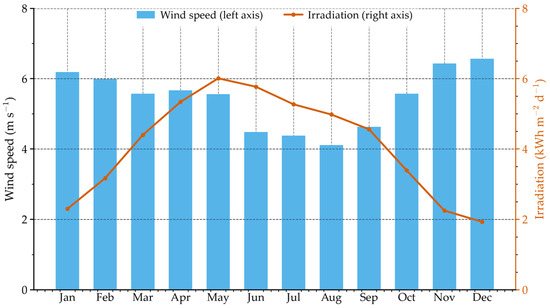
The monsoon cycle is pronounced: 6.57 m/s in December and 6.19 m/s in January, falling to 4.11 m/s in August. The seasonal range of the wind speed is a factor of 1.6, against 3.1 for the solar resource discussed in Section 2.3; the solar resource is therefore the more seasonal of the two. The two statements are reconciled by the energy they produce rather than by the resource ranges: because wind supplies most of the delivered energy, the seasonal range of the wind yield is the larger of the two in absolute terms, and it is the yield that Section 4.3 examines.
Wind speeds were represented by a two-parameter Weibull distribution, fitted month by month with a shape parameter k = 2. The corresponding scale parameter c is listed in Table 1 and refers to the 10 m height of the reanalysis variable; the transfer to the 8 m hub height is given in Section 3.2. This follows established practice for the China Sea resource assessment [18]; the sensitivity of the annual yield to the shape assumption is examined in Section 4.2. The monthly maximum 10 m wind speed reaches 16.7–20.3 m/s over the ten-year record (Table 1), well above the 13.8 m/s that the preliminary design basis treated as the survival wind speed. Winds up to Force 6 are thus a recurring strong-wind condition rather than a survival case, and the monthly maxima reach Force 8. The survival condition is taken here from the typhoon case (Section 2.4).
Table 1.
Ten-year monthly climatology of the wind and solar resource at the site (NASA POWER/MERRA-2, 2015–2024).
2.3. Solar Resource
The resource peaks at 6.01 kWh m−2 d−1 in May and falls to 1.93 kWh m−2 d−1 in December, a range of 3.1. This is the larger of the two seasonal ranges in the resource itself, the wind range being 1.6 (Section 2.2). It does not follow that the delivered energy is more seasonal than the wind because, in absolute terms, the wind contributes the greater share; Section 4.3 gives the energy result.
The phase relationship matters for Section 4.3. The wind minimum in July–August does not coincide with the solar maximum in May–June. By August, the irradiation has already fallen from 6.01 to 4.98 kWh m−2 d−1, while the wind resource is still declining, so the two are only partly complementary. This is worth anticipating here because the consequence is counter-intuitive and is carried through to the Conclusions: at this site, the array does almost nothing to flatten the annual energy profile, and the winter-wind/summer-sun compensation that hybrid systems are usually justified by does not hold. Both series are plotted in Figure 1.
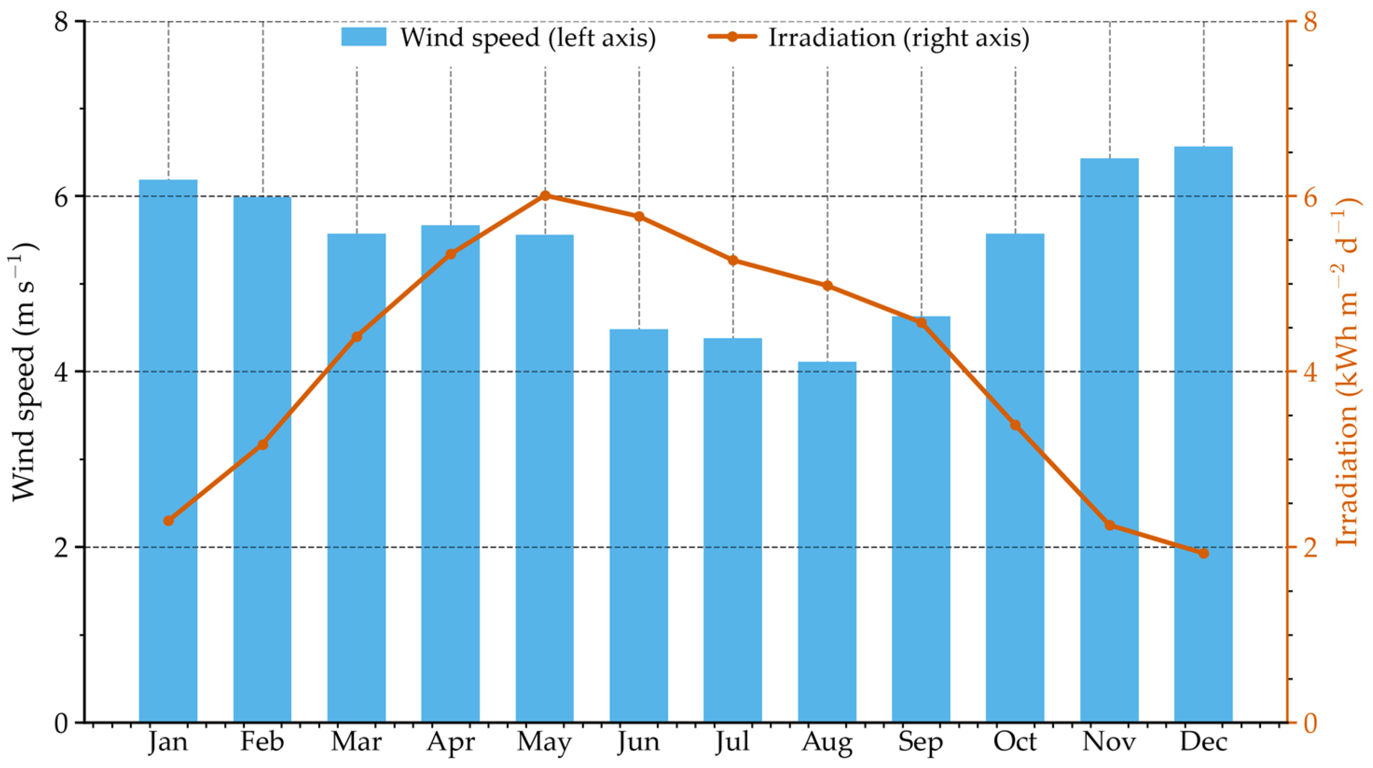
Figure 1.
Ten-year monthly climatology of the wind speed at 10 m (bars, left axis) and the horizontal surface irradiation (line, right axis) at the site.
2.4. Design Basis
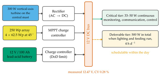
Figure 2 shows the system schematic. Table 2 collects the design parameters used throughout. Two differ from the preliminary design basis for this platform; both are justified below.
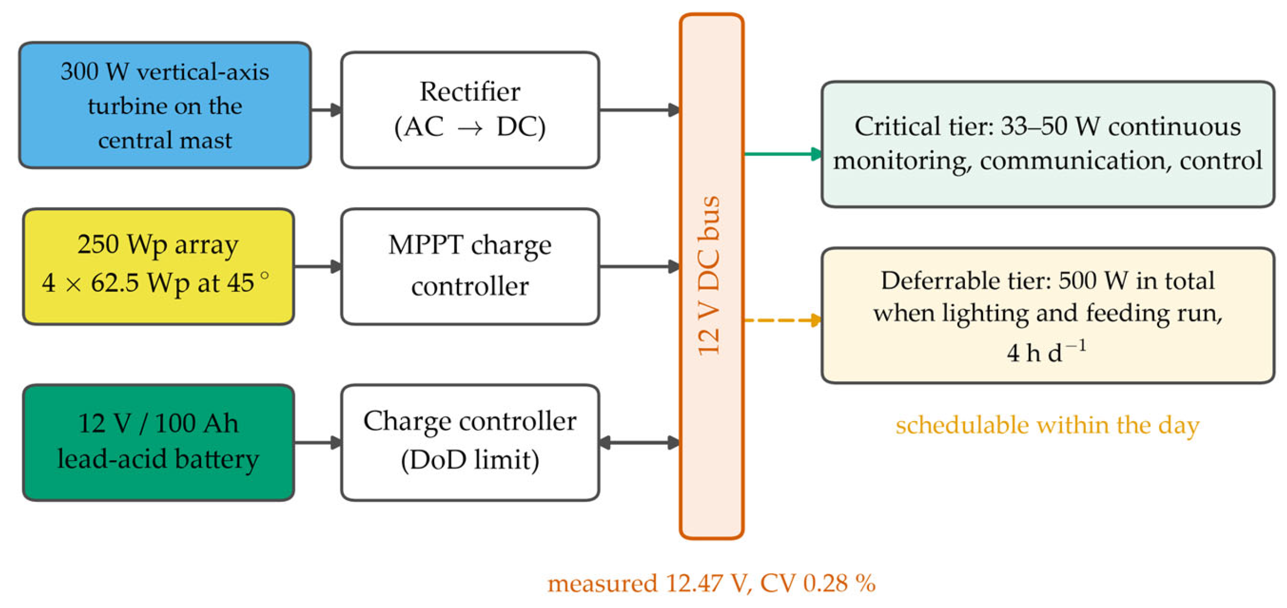
Figure 2.
System schematic. The turbine output is rectified, and the array is controlled before both reach the single 12 V DC bus; the battery sits on the bus through a bidirectional charge controller that enforces the depth-of-discharge limit. The critical and deferrable tiers are separate connections from the bus, which is what allows the deferrable load to be scheduled into hours of surplus generation.
Table 2.
Design basis derived from the resource and from the survival condition.
We retain the turbine rated wind speed at 6.0 m/s even though the ten-year annual mean is 5.43 m/s. Small vertical-axis machines are commonly specified at 6 m/s, and this one is rated at 300 W at that speed; the rated point is a property of the machine, not of the site. The consequence is that the turbine runs below its rated point for most of the year. It is quantified in Section 4, and it is why a design-point comparison is unsafe.
3. Stand-Alone DC Bus and Component Models
3.1. Configuration of the DC Bus and the Load Tiers
The buoy is an axisymmetric floating body of 0.9 m radius: a hemispherical base below the waterline and a cylindrical upper body above it. It is moored at a single point. A central mast carries the vertical-axis turbine. The internal compartment of the cylindrical body houses the battery and the power electronics. The prototype displaces 2.54 m3 at a total mass of 2603.5 kg. The nominal 0.75 m and the measured 0.78 m refer to the depth of the mooring attachment below the waterline, not to the draft. The displacement balance is closed here, because the geometry is easy to misread. A hemisphere of that radius displaces 1.527 m3 when fully submerged. The cylinder contributes the remaining 1.013 m3; at a waterplane area of 2.545 m2, that is 0.398 m of cylinder below the waterline, so the keel lies 1.298 m below it, and the waterline draft is about 1.3 m.
Three conversion stages connect the sources to the bus. The turbine produces alternating current at a frequency and amplitude set by the rotor speed, so its output is rectified before it reaches the bus. The rectifier has to accept an input voltage that varies widely with wind speed, because the turbine output changes as the cube of that speed between cut-in and rated. The four panels are connected in series-parallel and fed to the bus through their own charge controller. Both controllers operate at the maximum power point of their source, so the array is held at its maximum-power voltage as the irradiance and cell temperature change through the day. The converter losses are not modelled as a separate stage; they are carried in the performance ratio of Section 3.3, together with the other array-level losses listed there. The battery sits directly on the bus through a charge controller that limits the charging current and enforces the depth-of-discharge limit.
The battery sets the bus voltage. It is a low-impedance source across the bus, so the regulation reported in Section 6.2 reflects the charge/discharge balance of the lead-acid cells rather than an active voltage regulator. This matters for sizing: what has to be matched to the load is the energy delivered at the bus terminals after these stages, not the sum of the component ratings.
The load is not a single number. Following the operator’s description of the farm, we split it into two tiers (Table 3). The critical tier covers monitoring, communication, and control, draws 33–50 W, and must be supplied without interruption. The deferrable tier covers lighting and feeding and can be moved within the day. The two are not additive: 500 W is the total drawn when the lighting and feeding equipment runs together with the critical tier, so the deferrable increment is 450 W, not 500 W. The preliminary design treated the total of 500 W as a continuous demand and compared it with the 500 W design-point output; Section 5 shows what that comparison implied. Where a single figure is needed for the critical demand, we use the upper bound of 50 W, which makes the storage requirement quoted in Section 5 conservative.
Table 3.
Load tiers used in the analysis.
3.2. Turbine and Rectification
The turbine was modelled with a conventional three-region power curve. Below the cut-in speed, the output is zero. Between the cut-in and the rated speed, the output follows the cube of the wind speed. Between the rated and the furling speeds, the output falls linearly from the rated value to the value measured at the furling speed. Above the furling speed, the measured output falls as the overspeed protection acts, until cut-out:
where Pv is the turbine output at wind speed v, Prated is the turbine rated power, Pfurl is the turbine output at the furling speed, v is the wind speed at hub height (m s−1), vci, vr, vf, and vco are the cut-in, rated, furling, and cut-out wind speeds (m s−1).
The cut-in speed is 3.0 m/s, the rated speed 6.0 m/s at 300 W, the furling speed 12.0 m/s at approximately 150 W, and the cut-out speed 20.0 m/s. Above the furling speed, the output falls linearly to zero at cut-out, which follows the measured decay as the overspeed protection acts. At the 8 m hub height, the ten-year wind yield is 1171 kWh per year, which is the figure carried in Table 4. Wind speeds were referred from the 10 m reanalysis height to the 8 m hub height with a power-law exponent of 0.14. The transfer factor is 0.969.
Table 4.
Monthly and annual energy yield over the ten-year record, from the hourly model of Section 5.4. The right-hand column is the delivered energy as a fraction of a continuous 12 kWh/day demand; it is not the capacity factor, which is defined in Section 4.1 and reported there for both installation bases.
The model reproduces the measured operating point: 295 W was measured against 300 W modelled at the rated wind speed of 6 m/s, a difference of 1.7%. Only two measured points were available, at 6 m/s and at 12 m/s, so the shape of the curve between those anchors is adopted rather than validated. This is the dominant modelling uncertainty on the wind side, and it is examined in Section 6.3. Floating vertical-axis machines of this scale have been characterised numerically and in wind–wave basin tests [19].
3.3. Array and Charge Control
The array is rated at 250 Wp at standard test conditions and was modelled as PPV = PSTC × (G/GSTC) × PR. It is made up of four 62.5 Wp monocrystalline panels mounted symmetrically around the central mast, each inclined at 45° from the horizontal and facing outward, and the mounting is fixed rather than tracking. The 45° inclination is close to the angle that maximises annual yield at this latitude, and it also sheds spray and snow. Because the mounting is fixed to a floating body, the array orientation in service is the installed orientation superposed on the buoy’s roll and pitch. The four panels are mounted on one level about the mast, so they shade one another at low solar elevation; that array-level loss is carried in the annual performance ratio below rather than modelled separately. At the reference irradiance used throughout this study, 800 W m−2, the rating scaled by irradiance alone gives 200 W. Measured at that irradiance: 198 W, a difference of 1.0%. The reference point therefore validates the irradiance scaling of the array. Estimating the annual energy yield of a floating photovoltaic array from the rating and the incident irradiance is standard practice, and the loss channels it has to carry are well documented [20]. For the annual energy estimate, a performance ratio PR = 0.85 is applied. It carries the losses the reference measurement does not: a cell temperature above the 25 °C reference, with a temperature coefficient of −0.4% K−1 adopted for this module type, plus soiling, mismatch, cabling and the inter-panel shading noted above. The annual energy model also applies that temperature coefficient hour by hour (Section 5.4). The annual figures below should not be read as the reference-point output, which applies only while the reference irradiance persists.
We considered two corrections, both small for this platform. Wave-induced roll and pitch change the incidence angle of the direct beam, but at the working sea state—roll and pitch amplitudes of approximately 3.2° and 2.1°—the effect on this compact buoy body is about 0.1%, so it is neglected. Wave-induced motion losses of this order have been reported for other floating photovoltaic platforms [21,22]. The performance ratio is the dominant modelling uncertainty on the photovoltaic side: a range of 0.75 to 0.95 changes the annual photovoltaic yield from 282 to 357 kWh.
3.4. Battery and Usable Capacity
The battery is a 12 V/100 Ah lead-acid unit with a nominal capacity of 1.2 kWh. Lead-acid cells should not be taken below about 50% state of charge in routine cycling, so we use 0.6 kWh as the usable capacity in the autonomy calculations and quote the full 1.2 kWh only where stated. That 0.6 kWh is the capacity available at the terminals of the cells; once the discharge efficiency is applied, the energy actually delivered to the bus is about 0.54 kWh, which is the figure used in Section 5.3 and in the hourly model of Section 5.4. Discharging the full usable capacity of 0.6 kWh gives 12.0 h at the 50 W end of the critical range and 18.2 h at the 33 W end; Section 5.3 gives the realistic values at the adopted depth of discharge.
4. Annual Energy Balance and Capacity Factor
4.1. Method
For each month, the expected turbine output was obtained by integrating the power curve over the fitted Weibull distribution,
where is the monthly mean turbine output (W), f is the Weibull probability density function of the wind speed, and v is the wind speed at hub height (m s−1).
The monthly wind energy is Ewind = P × 24 × Ndays. The monthly photovoltaic energy follows from the rating, the monthly mean daily irradiation H and the performance ratio,
where EPV is the monthly photovoltaic energy (kWh), PSTC is the array rating at standard test conditions (Wp), H is the monthly mean daily irradiation as peak sun hours (kWh m−2 d−1), PR is the annual performance ratio, and Ndays is the number of days in the month. The factor 0.001 converts Wh to kWh.
Two capacity factors are used, and they should not be confused. The wind-side capacity factor of the month depends on what is taken as the installed rating. Against the reference design point of 500 W, which is the turbine at 300 W plus the array at 200 W at 800 W m−2, it is 33.8% over the ten years. Against the nameplate rating of 550 W, it is 30.7%. The second figure is the one that can be checked against the installed hardware, so both are given. The preliminary design point was matched to the load, so the design-point energy per day equals the daily demand of 12 kWh. The capacity factor on the 500 W basis and the fraction of the 12 kWh demand that is covered are therefore the same number, 33.8%. That equality holds only at the annual level. It does not hold month by month, and the two are reported separately in Table 4.
4.2. Monthly and Annual Energy Balance
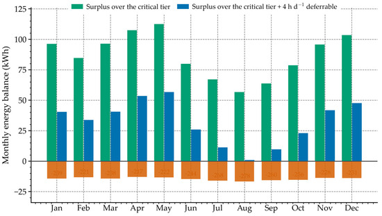
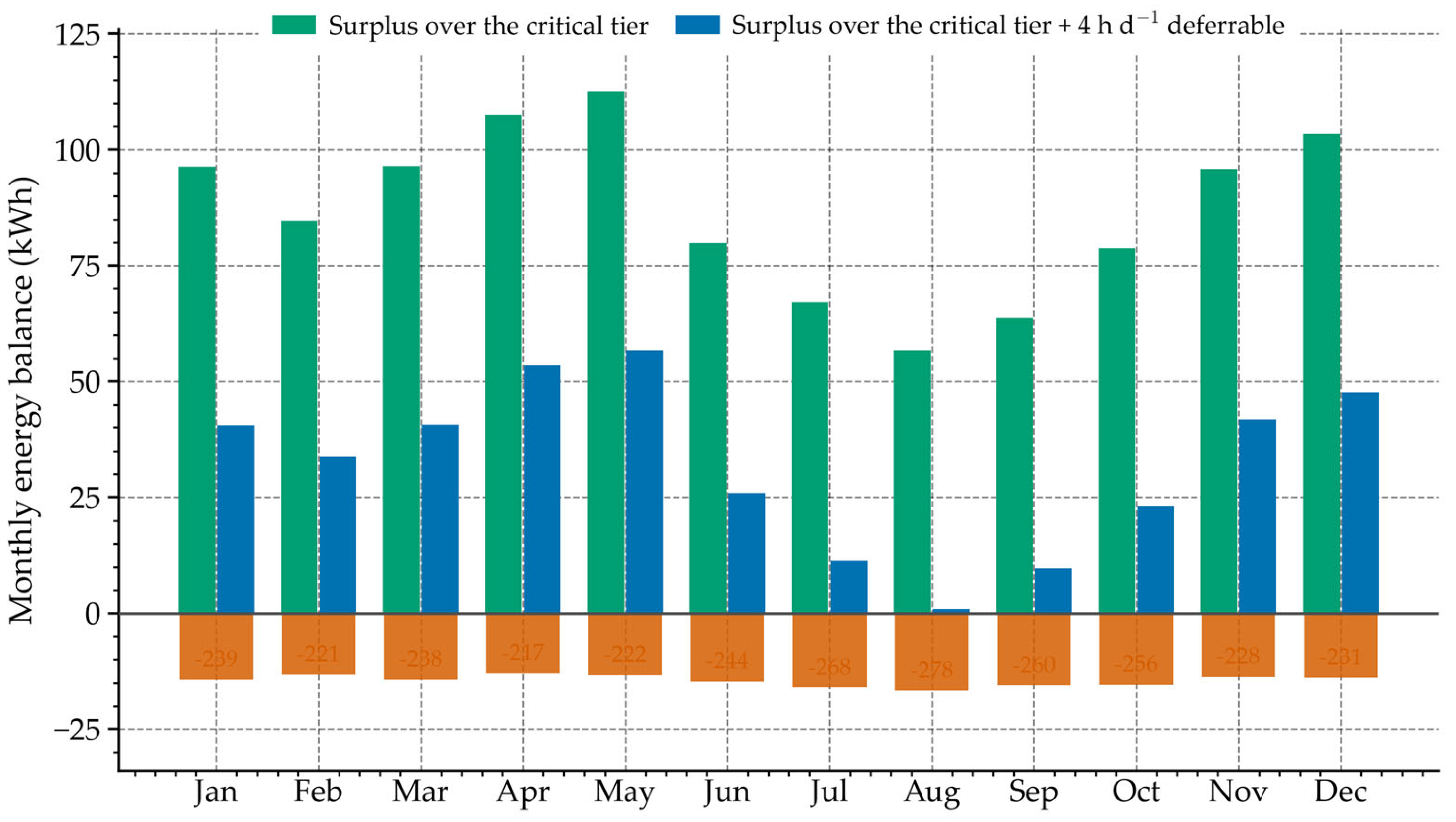
Table 4 gives the monthly result from the hourly model, and Figure 3 shows the delivered energy against the two load tiers month by month. The capacity factor and the coverage of the 12 kWh per day demand are reported as separate quantities there, and they coincide only at the annual level (Section 4.1).
Figure 3.
Monthly energy balance against the two load descriptions: the surplus over the critical tier, the surplus over the critical tier plus a four-hour deferrable schedule, and the shortfall against a continuous 12 kWh/day demand (bars below the axis, scaled by 0.06). Generation exceeds the critical tier in every month of the ten-year record; the margin is smallest in August (+57 kWh) and largest in May (+113 kWh).
The monthly model delivers 1464 kWh per year, of which 1144 kWh comes from wind and 319 kWh from photovoltaics, and it gives a mean daily delivery of 4.01 kWh and an annual capacity factor of 33.4% on the design-point basis. The ten-year hourly simulation of Section 5.4, which uses the same component models but the hourly resource directly, gives 1481 kWh per year over the ten years, of which 1171 kWh is wind and 310 kWh is photovoltaic. Both models run at the 8 m hub height. The wind figures differ slightly because the fitted Weibull distributions only approximate the hourly record, and the photovoltaic figures differ because the hourly model applies the cell-temperature coefficient hour by hour while the monthly model omits it. The two agree to within about 1%, so the monthly Weibull model is a sound annual estimator. Table 4 lists the hourly monthly figures, and the capacity factors quoted in Section 4.1 are those of the hourly model, 33.8% against the design point and 30.7% against the nameplate. Those are the figures carried through the rest of the paper where reliability is concerned. The installed rating is 300 W plus 250 Wp, but the design-point output at the reference conditions is 500 W, and it is that output sustained for a full year, 4380 kWh, which the design implicitly assumed. The supply delivers about 34% of it. An annual balance of this kind establishes the margin of the supply over the load; it does not establish that the load is served in every hour, and Section 5.4 shows that it is not.
The design-point balance describes a single instant of good resource, not a year: it holds only while the 6 m/s wind and the 800 W m−2 irradiance both persist, a small fraction of the time. Averaged over the record, the same hardware delivers 4.05 kWh per day, not 12, and that gap is what a design-point comparison conceals.
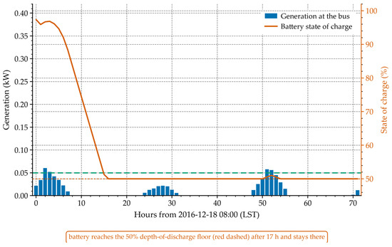
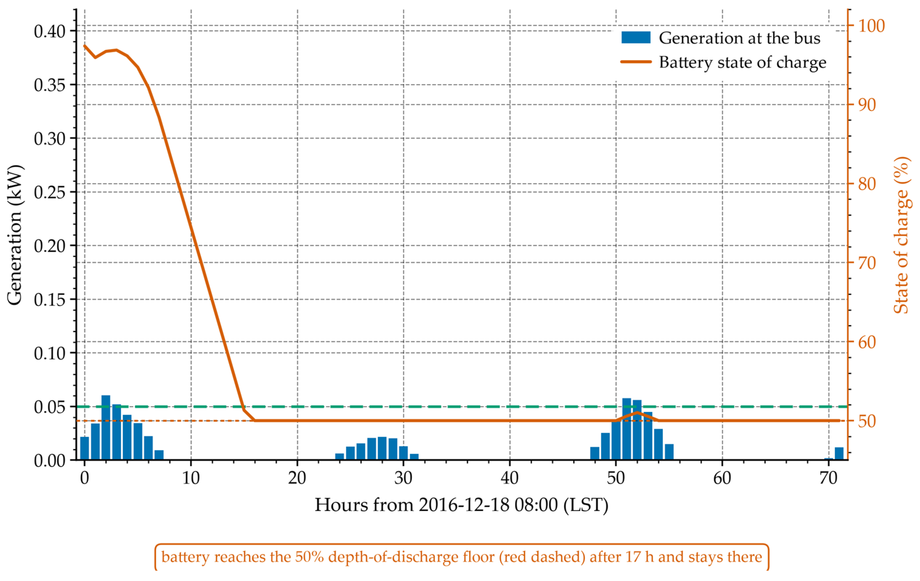
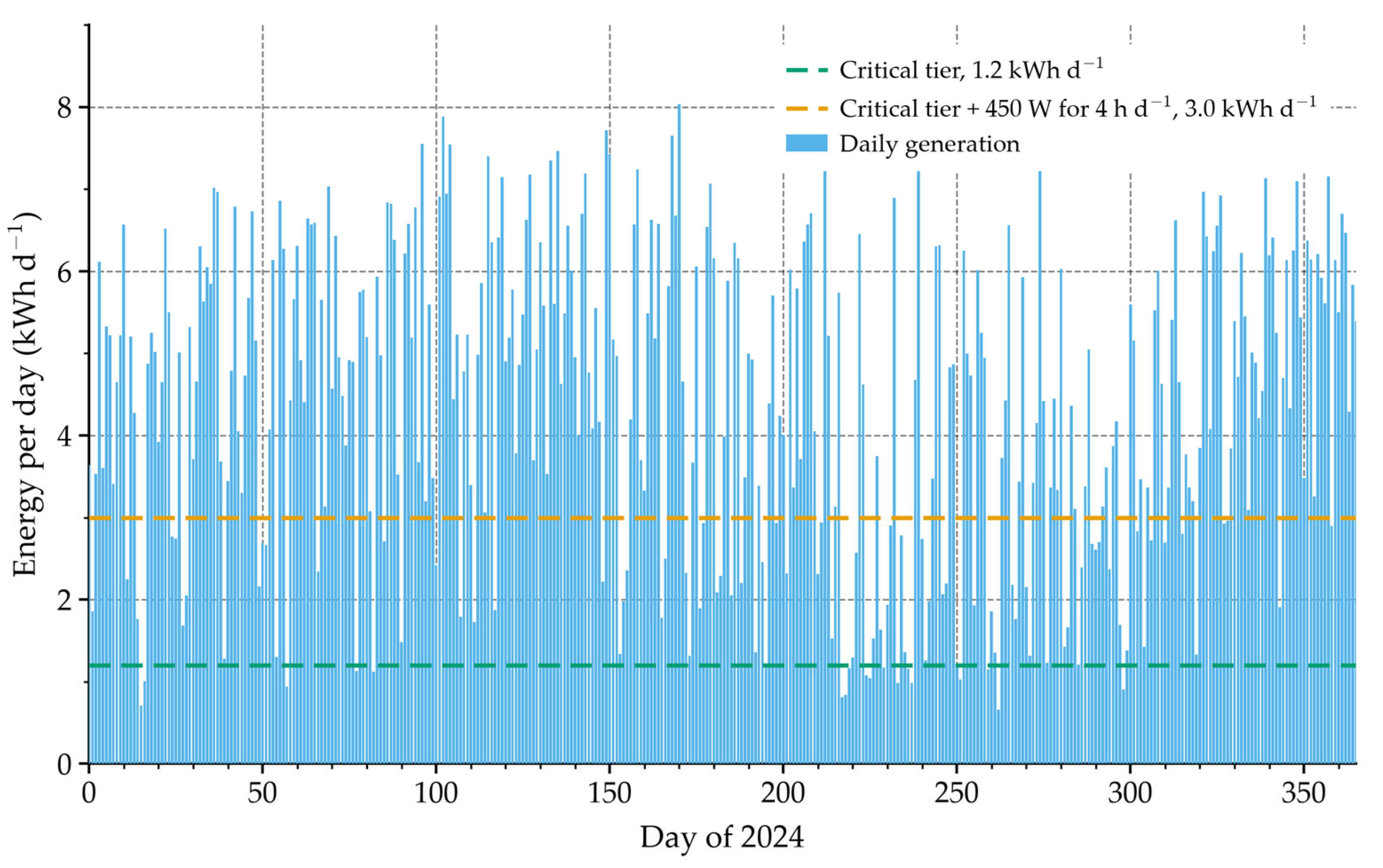
Over the ten years the monthly delivered energy varies by a factor of 1.59, from 4.83 kWh/day in May to 3.03 kWh/day in August (Table 4). The resource ranges are comparable or wider, 1.60 for the wind speed and 3.11 for the irradiation, but they are not directly comparable, because the wind supplies four fifths of the energy. The point that matters is that the delivered-energy ratio, 1.59, is no better than the wind-speed ratio, 1.60. The array does very little to flatten the annual profile at this site. The annual capacity factors are 33.8% against the design point and 30.7% against the nameplate. Figure 4 shows the worst 72 h of the ten-year record, in which generation totals 0.7 kWh against a demand of 3.6 kWh and the battery sits on its depth-of-discharge floor, and Figure 5 shows the daily generation of the record year, 2024, against the two load tiers.
Figure 4.
The worst 72 h of the ten-year record: hourly generation at the bus and the resulting battery state of charge. Generation totals 0.7 kWh over the window against a critical demand of 3.6 kWh, and the battery reaches its 50% depth-of-discharge floor within 17 h and remains there for most of the event. The green dashed line marks the 50 W critical load.
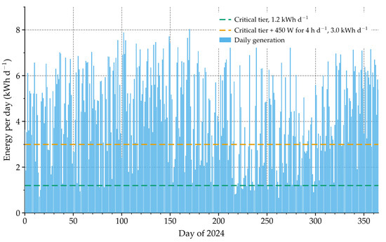
Figure 5.
Daily generation at the bus through the year 2024 of the record, against the critical tier and against the critical tier with the 450 W deferrable load running for four hours.
We tested two modelling assumptions. The first concerns the shape of the speed distribution. The power curve is convex below the rated speed, so the wind energy has to be obtained by integrating over that distribution; evaluating the power curve at the monthly mean wind speed instead overestimates the annual wind energy by 47%, 1687 kWh against 1144 kWh. The result is only weakly sensitive to the shape itself. Changing the Weibull shape parameter from the Rayleigh value of 2.0 to 1.8 or 2.2, at the same monthly means, moves the annual wind energy from 1144 kWh to 1093 kWh or 1199 kWh, a change of about ±5%.
The second assumption is the hub height. Reducing it from 8 m to 5 m at the same shear exponent lowers the turbine wind speed by 6.4% and the annual wind energy by 6.5%, to 1069 kWh. By comparison, a 10% change in the site wind speed changes the annual wind energy by about 9%, so the resource dominates the turbine model as a source of uncertainty. This sensitivity coefficient, close to unity rather than at the cubic exponent of the power curve, follows from the linear decline of the output between the rated and furling speeds and from the furling decay above them, which offset part of the cubic gain below the rated speed.
4.3. Seasonal Complementarity and Where It Fails
Hybrid wind–solar systems on this coast are usually justified by the argument that winter wind and summer sun compensate for each other, so that the combination achieves a higher capacity factor than either source alone [13,14,23]. The ten-year record supports the seasonal pattern, but not the conclusion.
Wind supplies 79% of the annual delivered energy and solar 21%, well away from the 60:40 split assumed in the preliminary design, which was not derived from any resource calculation. In August, the wind resource reaches its annual minimum of 4.11 m/s. The wind share falls, but the absolute yield does not recover. The solar resource is 4.98 kWh m−2 d−1, already 17% below its May peak. The array supplies 30.2 kWh in the month, against 37.7 kWh in May. The complementarity is real but weak. It does not prevent the August yield from falling to 3.03 kWh/day, the lowest of the year. Two consequences follow for the design. Because wind carries four fifths of the energy, a larger turbine would raise the annual total but would not help in August, when the wind resource itself is at its minimum; the machine and its support structure are also sized by the survival condition of Section 2.4, so upsizing the rotor is not a free change. A tracking array or an optimised orientation would move the annual split towards the 60:40 assumed at the design stage, but on a moored buoy that gain is bought with moving parts and additional wave-induced loads, and the fixed 45° mounting was chosen for robustness rather than for maximum yield.
A design based on annual energy absorbs this variation, because the battery and the load tiering carry it—but only within the limits of the store, and Section 5.4 shows that the limits bind. A design that assumed a constant 12 kWh/day shows a 75% shortfall in the same month. That is what follows from reading the design point as a delivered yield, and it is why the two quantities should be reported separately.
5. Storage Sizing and Load Coverage
5.1. The Load-Duration View
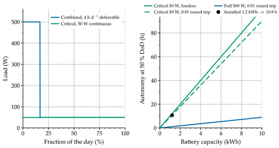
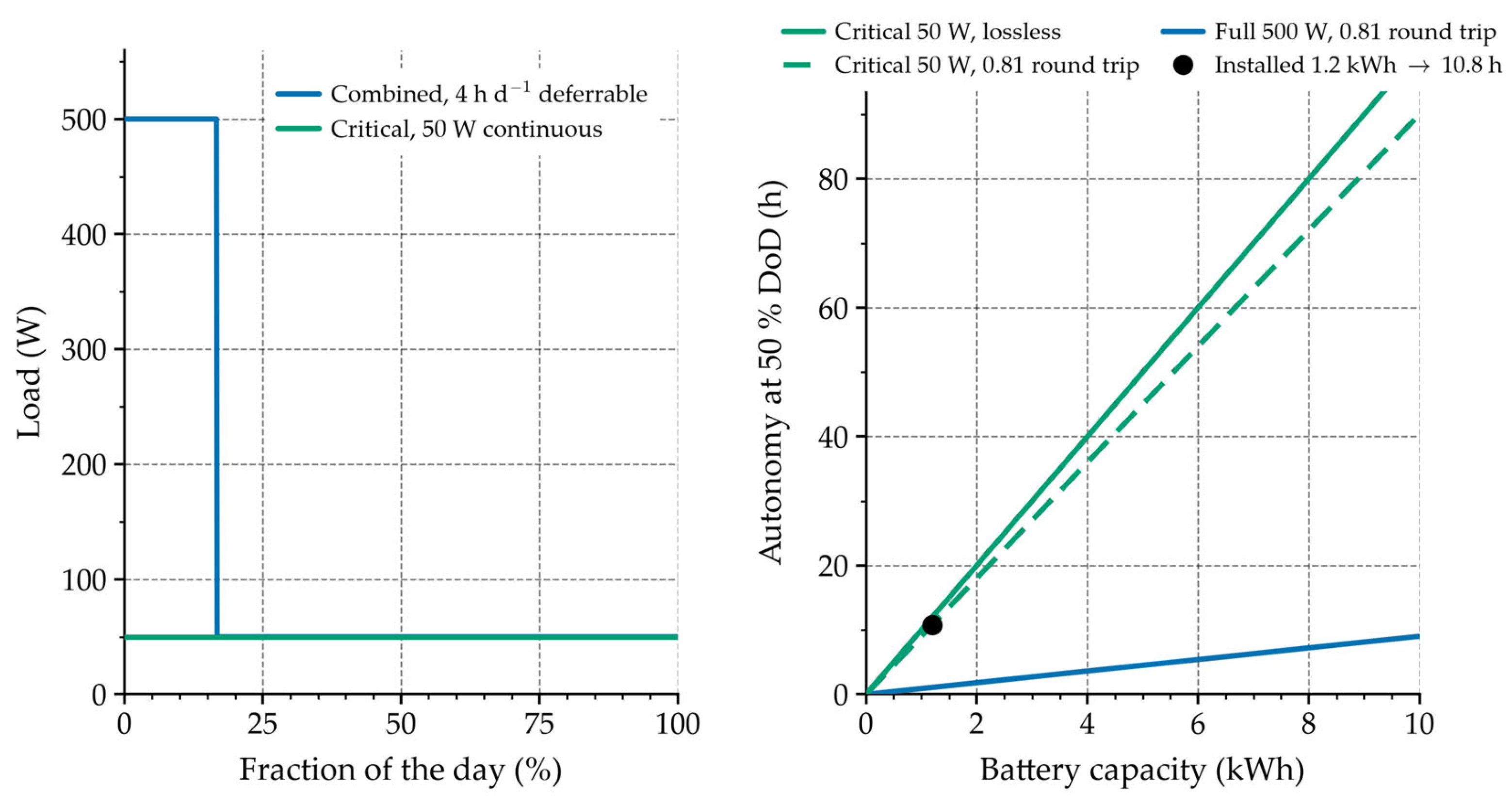
Figure 6 shows the two load tiers as duration curves. The critical tier is a flat 33–50 W, that is 0.8–1.2 kWh/day, and it sets the storage requirement because it cannot be deferred. The deferrable tier raises the demand to 500 W when it operates, which is an increment of 450 W over the critical tier and not a load additional to it. Its duration is not fixed by the farm operation but can be scheduled, which is what makes the tiering useful. We assume four hours of deferrable load per day, representative of a lighting and feeding schedule. Feeding dominates the electrical load at offshore cage farms, and such sites are normally off-grid and diesel-supplied [24]. Automatic feeders at comparable sites draw a few tens of watts rather than hundreds [24]. Continuous monitoring and communication at a comparable aquaculture site is met by a 50 Wp array with a 480 Wh battery at a reliability index of 100% [25]. Energy audits of Mediterranean sea-cage farms show direct energy use dominated by fuel, with only a minor electrical share [26]. Modelling lighting plus feeding as up to 500 W for four hours a day, about 2 kWh/day, is therefore on the conservative side. Load prioritisation of this kind is standard practice in isolated microgrid design, where scheduling the deferrable demand is what allows a smaller installation to meet the critical load [13,14].
Figure 6.
Left: load-duration curves for the critical tier and for the combined tier with four hours per day of deferrable load; scheduling the deferrable load cuts the time for which the full 500 W must be supplied from 100% to 17%. Right: autonomy against battery capacity at a 50% depth of discharge without the round-trip loss, for the critical and full tiers, with the installed 1.2 kWh battery marked.
5.2. Annual Load Coverage
The critical demand is 50 W × 24 h × 365 = 438 kWh/year. The 1481 kWh/year delivered covers it 3.4 times over in energy, so the critical tier is covered in annual energy with a wide margin. That is a statement about the annual balance, not about continuity. The same 3.4-fold margin coexists with a residual shortfall hour by hour, and Section 5.4 quantifies it. The full-tier demand is 500 W × 24 h × 365 = 4380 kWh/year, of which the delivered energy covers 34%.
The verdict therefore depends entirely on how the load is described. Against the critical tier alone, the supply covers 338% of demand; against the critical tier plus the four-hour deferrable schedule of Section 5.1, it covers 135%; against a continuous 500 W demand, it covers 34%. One set of hardware supports all three readings. A comparison of component ratings distinguishes none of them, so any sizing procedure for this class of supply has to begin from a load-duration description.
5.3. Autonomy and the Sizing Rule
Table 5 gives the autonomy obtained from a given battery capacity on each tier at a 50% depth of discharge, with the round-trip loss applied. Figure 6 shows the same information graphically, together with the load-duration curves.
Table 5.
Autonomy as a function of battery capacity and load tier at a 50% depth of discharge, with the round-trip loss of 0.81 applied. The lossless column is given for comparison so that the size of the correction is visible. The cycle count is from the hourly simulation at the installed capacity.
On the critical tier, the installed 1.2 kWh battery gives 10.8 h at a 50% depth of discharge once the discharge efficiency is carried, and 24 h at a full discharge. The preliminary design assumed 24–36 h from the same battery; that figure is correct only at a full discharge and for a load at the bottom of the critical range. At a realistic depth of discharge, it is 10.8–16.4 h, the upper figure being the 33 W end of the critical range. Restoring 36 h of autonomy on the critical tier at 50% depth of discharge requires 4.0 kWh once the losses are carried, against the 3.6 kWh that a lossless calculation gives, and the extra storage costs far less than the additional generation that would be needed to make the full tier continuous. Sizing storage from the demand profile rather than from a single power figure has been shown to reduce the installed capacity of isolated systems [27].
A design rule follows, and it transfers to other sites, but it is a preliminary rule, and it sets a lower bound rather than a complete specification. The battery is sized for the critical tier at the required autonomy and depth of discharge. The generation is sized for the annual energy of the critical tier, plus as much of the deferrable tier as the resource can supply. The deferrable tier is scheduled into the resource window instead of treating it as a continuous load. Applied to this system, the rule gives 1.2 kWh of storage, or 10.8 h of critical autonomy once the discharge efficiency is carried, and 1481 kWh of annual generation. That covers the critical tier in energy terms three times over and the four-hour deferrable schedule in energy terms as well. The critical tier takes 438 kWh of the 1481 kWh, leaving 1043 kWh per year for the deferrable tier, which is 6.4 h per day at the 450 W increment. It is against the preliminary basis of a continuous 500 W demand that the same supply covers only 34%. The rule accounts for energy, not for continuity, and the two differ: because the rule sizes the store from the critical load and the depth of discharge, it cannot guarantee that the store bridges the longest lull in the record. Section 5.4 quantifies the residual and shows what it takes to remove it.
5.4. Hourly Reliability of the Critical Tier
The energy balances above compare monthly energies. They cannot show whether the critical tier is served in every hour, and this is the claim that matters. An hourly model was therefore built over the whole ten-year record, 87,672 h. The hourly wind speed at 10 m, the all-sky surface shortwave irradiance and the 2 m air temperature were taken from the same NASA POWER archive used in Section 2. They were referred to the 8 m hub height with the same shear exponent, then passed through the turbine curve of Equation (1) and the array model of Section 3.3, including the cell-temperature derating. The battery was modelled as a state of charge with a round-trip efficiency of 0.81 and a hard floor at 50% depth of discharge. The critical tier is served first in every hour. The deferrable tier is dispatched in two ways because the choice turns out to matter, and the total is capped by what the sources can deliver.
The dispatch rule is stated here because the reliability figures depend on it. In every hour, the critical tier is served first from generation and, when that is not enough, from the battery. The deferrable tier is then treated in one of two ways. Under the scheduled policy, it runs for four hours each calendar day, placed in the four hours of highest generation of that day. Under the surplus-only policy, it runs only in hours in which generation already covers the critical tier and the battery is not being discharged. Surplus energy charges the battery at a constant one-way efficiency of 0.90, and discharge is subject to the same efficiency, so the cycle round-trip efficiency is 0.81. Charging is limited by the remaining capacity of the store and discharge by its state of charge. The store is initialised full at the start of the ten-year record and carries its state of charge continuously through it; it may not fall below 50% depth of discharge, which fixes the floor of 0.54 kWh delivered to the bus. The deferrable load is shed rather than the critical load whenever the two cannot both be met.
Over the ten years, the hourly model delivers 1481 kWh per year at the bus, a mean of 4.05 kWh per day, in agreement with the monthly model to within about 1%. Generation exceeds the 50 W critical load in 76.6% of hours, so that in the remaining hours the load is carried entirely by the battery. The longest run of consecutive hours in which generation stays below the critical load is 47 h, against a battery autonomy of 10.8 h; the second and third longest are 42 h and 37 h, and the 95th-percentile run is 16 h. Table 6 gives the resulting reliability, and Figure 4 shows the worst 72 h window of the record, in which generation totals 0.7 kWh against a demand of 3.6 kWh and the battery sits on its depth-of-discharge floor for most of the event. The daily generation falls below the critical daily demand of 1.2 kWh on 295 of the 3653 days of the record. The duty cycle of the deferrable load is an operating assumption, and Table 7 shows that the result does not turn on it: doubling the deferrable duration to 6 h per day, or halving it to 2 h, moves the unmet critical energy by about two percentage points.
Table 6.
Hourly reliability of the critical tier over the ten-year record (87,672 h). The critical demand is 50 W continuous, 438 kWh per year. “Surplus only” dispatches the deferrable load only in hours in which generation already covers the critical tier; “fixed 4 h/day” runs it for four scheduled hours each day. Coverage is the complement of the unmet fraction. The 0.72 row is the round-trip efficiency of the aged cell, given for comparison.
Table 7.
Sensitivity of the result to the assumed duration of the deferrable load, at a round-trip efficiency of 0.81 and with the deferrable load on a fixed daily schedule. The four-hour case used throughout the paper is the middle of the range.
The critical tier is not covered without interruption. With the deferrable load restricted to surplus hours, 2.65% of the critical demand is unserved in 3.8% of hours. Running the deferrable load on a fixed four-hour schedule raises that to 8.35%. The reason is simply that both tiers then draw on the same stored energy. The dispatch rule for the deferrable tier is therefore worth about 5.7 percentage points of critical-tier coverage, which is a larger effect than any component change examined here.
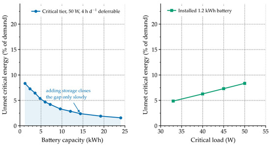
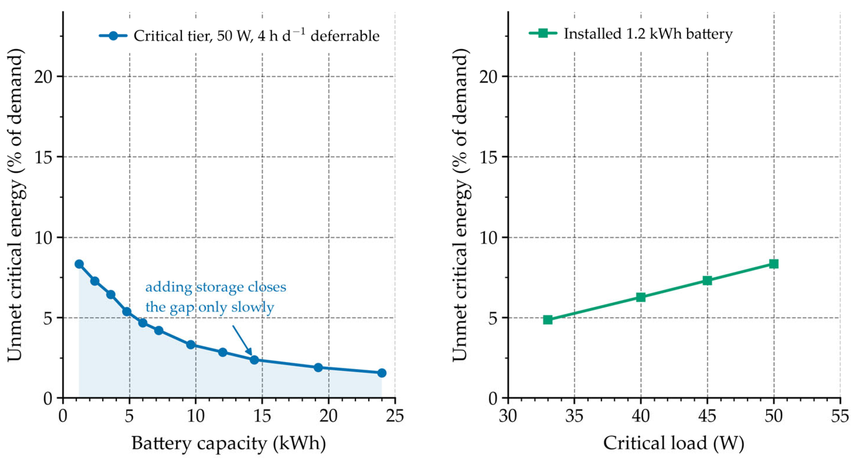
The shortfall is set by usable capacity, not by the annual resource. Even if the entire generation passed through the battery, 1199 kWh per year would remain after the round-trip loss, 2.7 times the 438 kWh critical demand. With an ideal store and no depth-of-discharge floor the critical tier is served in full. The installed battery holds 1.2 kWh, of which 0.6 kWh is usable at the 50% limit. That is half of one day of critical demand, and it cannot bridge a 47 h lull. Adding storage helps only slowly. Under the fixed four-hour schedule, raising the capacity to 3.6 kWh leaves 6.4% unserved, 9.6 kWh leaves 3.3%, and even 24 kWh still leaves 1.6%. The residual follows the timing of the longest lulls rather than the total energy. Figure 7 shows both responses.
Figure 7.
Left: the unmet critical energy against battery capacity, from the hourly model under the fixed four-hour deferrable schedule. Adding storage reduces the shortfall only slowly: 3.6 kWh gives 6.4%, and 24 kWh still leaves 1.6%. Right: the same quantity against the critical load at the installed 1.2 kWh capacity, showing that taking the lower end of the critical range (33 W) rather than the upper end (50 W) reduces the shortfall from 8.4% to 4.9%.
The limitation of the hourly model is the resource itself. It is driven by reanalysis rather than by an on-site measurement, so its absolute reliability figures inherit the uncertainty of Section 6.3. What does not depend on that uncertainty is the qualitative result: under the fixed four-hour schedule, across a wind bias of −15% to +15%, the unserved critical energy runs from 13.4% to 5.3% and never reaches zero, so annual energy adequacy does not imply continuity anywhere in the plausible range.
6. Field Validation
6.1. Prototype and Instrumentation
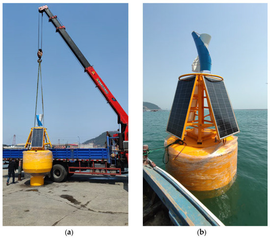
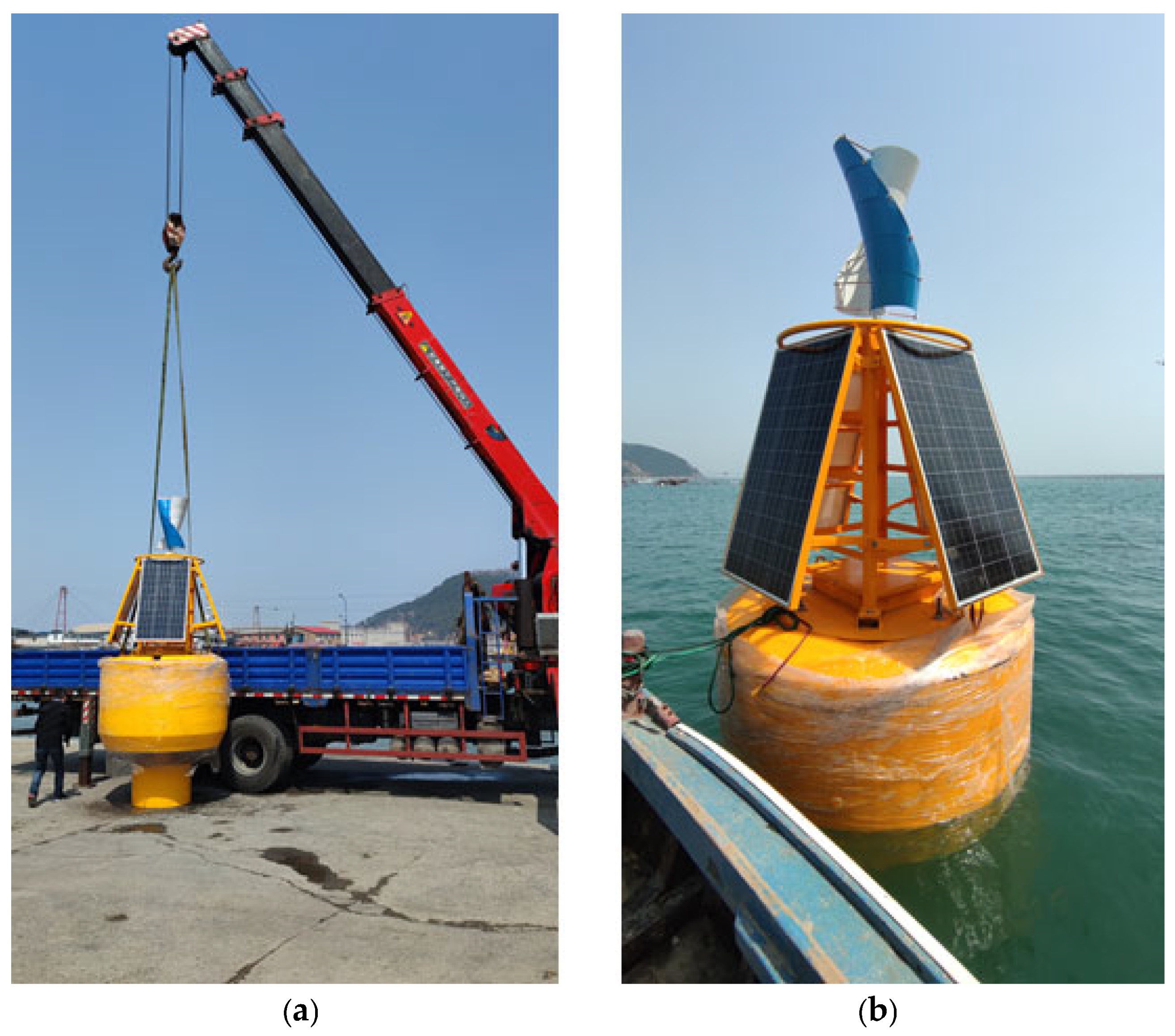
A full-scale prototype was built with a high-strength polyethylene body: a hemispherical base and a cylindrical upper section, with high-density rubber seals, a 300 W vertical-axis turbine on a central mast, four 62.5 Wp monocrystalline panels mounted around the mast at 45°, and a 12 V/100 Ah battery in the internal compartment. The body was thermoformed, and the compartments were assembled with bolted connections and sealing compound. Figure 8 shows the buoy being placed and the tow to the test location.
Figure 8.
Field records from the deployment. (a) The prototype being placed, with the turbine, array and cylindrical body visible; (b) the buoy under tow to the test site with the mast and modules erected. Both are documentary rather than measurement records, and the original files are of limited resolution.
The trials were carried out at Bailanzi Fishing Port, Lvshunkou District, Dalian, under real marine conditions, in May 2024, over three days for a total of about 9 h on station, and the prototype was assessed against the General Technical Specifications for Buoys, JT/T 760-2009 [28]. The water depth at the test site was 12 m, and the sea state was slight, with an estimated significant wave height below 0.3 m. The electrical measurements were taken with the prototype on load: the turbine and array were connected to the bus, and the critical tier was drawing its normal 40 W during the logging runs, so the bus voltage reported below is an on-load value. Bus voltage was logged at 1 Hz with a Fluke 287 multimeter (±0.025% + 5 digits), chamber pressure at 1 Hz with a digital manometer (±0.1% of full scale), and inclination at 20 Hz with a dual-axis inclinometer (±0.1°); all instruments were calibrated before use. Turbine output was obtained from the rectifier output current and the bus voltage. Ambient wind speed and irradiance were not logged on site, so the conditions referred to below are the reanalysis values for the test hours. We treat this as a limitation, not as a measurement (Section 6.3).
6.2. Comparison with the Model
Table 8 compares the modelled and measured quantities.
Table 8.
Modelled and measured quantities, with the relative difference on each basis. All measured values are on load, with the critical tier drawing its normal 40 W.
The turbine delivered 295 W at its rated speed against 300 W modelled, and the array 198 W at the reference irradiance against 200 W, with the test-hour wind speed and irradiance taken from the reanalysis (Section 6.1). The power curve is anchored on both measured points, 295 W at the rated speed of 6 m/s and about 150 W at the furling speed of 12 m/s, with a linear transition between them; the shape of the curve between the anchors is adopted rather than validated. The natural roll period was 2.82 s against 2.86 s from the hydrodynamic model, and the mooring attachment depth was 0.78 m against a nominal 0.75 m. The bus voltage averaged 12.47 V over eight readings with a coefficient of variation of 0.28%, a range of 12.42–12.53 V, or −0.64% to +0.24% of the 12.5 V nominal value. The chamber sealing test pressurised the compartment to 0.05 MPa and held it for 10 min in three trials; no pressure loss exceeding the instrument resolution of ±0.05 kPa was detected.
The relative differences are given on both bases. The attachment-depth comparison falls just below 4% with the measurement as denominator and just above it with the model as denominator; reporting only the first basis, as is common, would conceal that the agreement is at the 4% level rather than below it.
6.3. Uncertainty Budget
Table 9 gives the measurement uncertainty budget. Type A contributions are the standard error of the repeated readings. Type B contributions are taken from the instrument specifications and, for the resource, from an estimate of the difference between reanalysis and on-site conditions; those two rows are assumptions rather than measurements and are labelled as such.
Table 9.
Measurement uncertainty budget.
The combined bus voltage uncertainty is 0.12%, about a factor of two below the observed coefficient of variation of 0.28%. Measurement error therefore accounts for only part of the observed spread; the rest is real variation in the charge/discharge balance of the cells. The rolling-period uncertainty of 0.49% lies well below the 1.4% difference between the simulated and measured values, so that comparison is meaningful. The attachment-depth uncertainty of 1.3% is comparable to the 3.8% difference from the nominal value, so the attachment-depth agreement should be described as consistent rather than close.
The resource dominates the energy result, and it carries the largest uncertainty in the paper. A 15% uncertainty in wind speed moves the annual energy by −14.9% to +9.8% (Table 10), and a 12% uncertainty in irradiation moves it by about ±2%, because the array supplies only a fifth of the total. The two are independent and combine in quadrature to about −15% and +10%, or 1481 −224/+150 kWh per year; the response is asymmetric because the turbine saturates and furls at the upper end of the wind-speed range. The magnitudes are assumed, not measured. Their basis is as follows. Over the Bohai and Yellow Seas, reanalysis 10 m wind speeds reproduce buoy observations at twelve stations over eleven years with a correlation above 0.83 for speed and above 0.90 for direction [29]. For irradiance, NASA POWER daily solar radiation has been validated against ground stations with a normalised RMSE of 8–20%, and 11.2% for daily irradiation after bias correction [30]. ERA5 overestimates the national mean surface solar radiation over China by about 10 W m−2, roughly 6% [31]. The adopted values sit within those ranges. They are central estimates, not upper bounds, because the irradiance studies report normalised errors above 12% as well as below it. They are also single-source annual-mean figures. Extreme events would need a separate bias correction before the survival condition is used for structural design. The response to the assumption is reported as a range. The hourly model of Section 5.4 was rerun with a wind bias from −15% to +15% and an irradiance bias from −12% to +12% (Table 10, under the fixed four-hour deferrable schedule). The annual energy moves from 1260 to 1626 kWh/year, and the unmet critical energy from 13.4% to 5.3%. Both qualitative conclusions hold across the whole range. The resource, rather than the hardware, is what has to be measured. A short on-site reference campaign would replace the assumption with a measurement.
Table 10.
Response of the result to the assumed resource uncertainty. The annual energy and the unmet critical energy are from the hourly model of Section 5.4 with a uniform bias applied to the wind speed or to the irradiance across the whole record, under the fixed four-hour deferrable schedule.
6.4. Motion Response and Stability
A hydrodynamic model of the buoy was built in ANSYS AQWA-LINE 2023 R1 with the JONSWAP spectrum (γ = 3.3, σ = 0.07 below and 0.09 above the peak frequency), a water depth of 40 m, representative of the open-water design site rather than the 12 m harbour depth at which the trials ran, a 50 m × 50 m diffraction-mesh domain, a simulation of 200 s at a time step of 0.05 s, and first- and second-order wave forces. A mesh-convergence study used 8432, 16,894, and 33,786 elements. The heave RAO peak differed by 4.5% between the coarse and fine meshes and by 1.8% between the medium and fine meshes. A difference below 2% was adopted as the convergence criterion, and the medium mesh was used.
The model gives a natural roll period of 2.86 s (0.35 Hz) and a heave natural period of 2.50 s (0.40 Hz), both below the dominant wave period band of the site, 4.5–4.8 s. The resonant peaks are therefore not excited by the incident wave spectrum, and the buoy does not resonate at the design sea states; the frequency-domain response and the radiation coefficients are not reproduced here. What matters is that separating the natural periods from the wave band keeps the roll and pitch amplitudes small, which is the condition under which the incidence-angle correction discussed in Section 3.3 remains negligible. Parked and operating loads on floating vertical-axis machines have been measured in wind–wave basin tests, the closest available analogue to the sea trials reported here [32].
The small-angle free-decay records oscillate at about 1.4 s, against the 2.82 s measured in the 15° decays, and we report this amplitude dependence as an unresolved feature of the records rather than attribute it. As for the cause, the sampling rate can be addressed from the logging configuration. The inclinometer recorded at 20 Hz, which resolves the 1.4 s oscillation with about 28 samples per cycle, so the sampling rate was sufficient to resolve the short-period records and aliasing is not the explanation. That leaves the contamination of the small-angle decays by coupled heave motion or by the mooring as the most probable cause, and it is the mechanism we adopt here. A repeat campaign with the raw time series retained at a higher rate would settle it.
The waterline draft of about 1.3 m, fixed by the mass-displacement closure of Section 3.1, exceeds the 0.70 m minimum of JT/T 760-2009; the measured 0.78 m refers to the depth of the mooring attachment, not to the draft. The standard also specifies a rolling period of 3–5 s, and the measured natural period of 2.82 s lies below that band. The requirement appears to be written for navigation buoys, whose freedom of motion is not constrained; a shorter natural period is not in itself a defect here, since it moves the resonance away from the wave band rather than towards it. We therefore report the deviation explicitly instead of claiming compliance, and note that no dedicated criterion exists for small energy buoys. A still-water free-decay test cannot in any case demonstrate compliance with a maximum-inclination requirement, which is set by wind and waves in service; the tests establish the natural period, not the in-service inclination.
7. Discussion
The central result is that adequacy is a property of the load description, not of the hardware. The same supply covers a 50 W critical load 3.4 times over in annual energy, covers a four-hour daily deferrable schedule as well in energy terms (135%), and covers only 34% of a continuous 500 W demand; nothing about the hardware differs between the verdicts, only the assumption about the load. A design point is a power, and a demand is an energy, and equating the two is what produces the apparent factor of three. This distinguishes the present result from established stand-alone sizing practice. Capacity-optimisation tools, whether the standard simulation-based packages or the metaheuristic and multi-objective formulations now common in the literature [10], minimise a cost or maximise a reliability index over candidate capacities; all of them require a load profile as an input, usually a peak and a daily energy. The result here is that the same physical load, written down in three defensible ways, produces a tenfold range in the answer, which is an input those methods take as given rather than test. The contribution is therefore not a better optimiser but a demonstration that the load description dominates the sizing outcome, and the hourly evidence that fixing the description is not sufficient on its own either. The distinction from established practice is one of position rather than of method: those approaches answer the question “how much capacity, given this load”; the present result shows that the answer moves by an order of magnitude according to how that same load is written down.
The seasonal result deserves stating plainly, because it contradicts an assumption often used to justify hybrid systems [7,8]. The two resources at this site are out of phase, but the phase difference is too small to flatten the annual profile: delivered energy varies by a factor of 1.59 between May and August, which is no better than the 1.60 of the wind speed alone, and August is the minimum rather than the maximum, because the mid-summer wind lull is deeper than the mid-summer solar gain. A hybrid supply on this coast inherits the wind seasonality more than it compensates for it, and the 79% wind share reflects that. It has to be checked against the resource data; it cannot be assumed.
The limitations are set by the data, not by the model. No meteorological mast was deployed, so the resource comes from a reanalysis with a grid spacing of about 50 km. The resulting 15% uncertainty in wind speed becomes −14.9% to +9.8% in annual energy, and about −15% to +10% in the annual total (Table 10). That is larger than every other uncertainty in the study combined, and it is the strongest argument for a short on-site reference campaign. The turbine power curve is the second soft point: only two operating points could be logged, so the shape between cut-in and rated speed had to be adopted. The campaign itself lasted hours rather than months, so nothing can yet be said about ultraviolet degradation of the polyethylene body, marine growth on the panels, or calibration drift, and the seasonal losses these would cause are absent from the annual model. The survival condition of 6.5 m significant wave height and 32 m/s was never encountered, so it is carried in the design basis only. No cost model was built, and without one the tiering argument cannot be weighed against the 2–3 RMB per kWh that operators pay for diesel. Finally, the small-angle rolling records remain unexplained, and we report them as such.
The sizing rule generalises, but only as a lower bound. Resource statistics give the annual energy; the load-duration curve, not the peak load, sets the storage; and the deferrable part of the load should be scheduled rather than sized for. The hourly analysis qualifies it: the same supply leaves 2.65–8.35% of the critical demand unserved, because the usable capacity at a 50% depth of discharge is half of one day of critical demand and the longest lull in the record is 47 h. The rule therefore specifies a system that is adequate on annual energy and not yet adequate hour by hour, and closing that gap is a storage and dispatch decision rather than a generation one.
8. Conclusions
We sized a stand-alone wind–photovoltaic DC supply for an offshore cage farm and validated its component models against a full-scale prototype (differences of 1.7%, 1.0%, and 1.4% for the turbine, the array, and the roll period). The supply delivers about 1481 kWh per year, and whether that is enough is a property of the load description rather than of the hardware: the same installation covers a 33–50 W critical load 3.4 times over in annual energy, yet only 34% of the continuous 500 W reading it was originally matched to. Annual adequacy does not imply continuity: hour by hour, 2.65% of the critical demand remains unserved under surplus-hour scheduling and 8.35% on a fixed schedule; the longest lull of 47 h outlasts the 10.8 h of battery autonomy, and 24 kWh of storage still leaves 1.6% unserved. The two resources are out of phase but only weakly complementary: the winter-wind/summer-sun compensation often assumed for hybrids does not hold on this coast, because the August minimum of 3.03 kWh/day falls inside the wind lull rather than against the solar peak, so generation and storage must both be sized for the wind season and the array treated as an energy contributor. Uncertainty is dominated by the reanalysis resource (−15% to +10% on the annual energy), and the three-day trials leave seasonal degradation, biofouling and calibration drift unrepresented. The next step is a techno-economic study that prices the storage for the critical tier, the generation avoided by scheduling the deferrable tier (roughly a fourfold saving) and the residual shortfall, against the 2–3 RMB per kWh that operators now pay for diesel, alongside a short on-site meteorological reference, a full turbine power curve and multi-season trials.
Author Contributions
Conceptualisation, Y.Z. and G.M.; methodology, Y.Z. and G.M.; software, Y.Z.; validation, Y.Z., G.M., H.C. and F.D.; formal analysis, Y.Z.; investigation, Y.Z.; resources, G.M.; data curation, H.C.; writing—original draft preparation, Y.Z.; writing—review and editing, G.M., H.C. and F.D.; visualisation, Y.Z.; supervision, G.M.; project administration, G.M.; funding acquisition, H.C. All authors have read and agreed to the published version of the manuscript.
Funding
This research was funded by the Natural Science Foundation of Liaoning Province (grant number 2024BSLH258) and the Scientific Research Project of the Liaoning Provincial Department of Education (grant number LJ212510153047).
Data Availability Statement
The NASA POWER reanalysis data used in this study are openly available from https://power.larc.nasa.gov/. The field measurement data are available upon request from the corresponding author.
Acknowledgments
The authors thank the marine meteorological services in Dalian for the environmental data, and the crew of Bailanzi fishing port for assistance with the sea trials.
Conflicts of Interest
The authors declare no conflicts of interest.
Abbreviations
AQWA, ANSYS Quantitative Wave Analysis; CV, coefficient of variation; DoD, depth of discharge; JONSWAP, Joint North Sea Wave Project; LST, local solar time; MERRA-2, Modern-Era Retrospective analysis for Research and Applications, version 2; MPPT, maximum power point tracking; NASA POWER, Prediction of Worldwide Energy Resources; PR, performance ratio; PV, photovoltaic; RAO, response amplitude operator; SoC, state of charge; STC, standard test conditions; VAWT, vertical-axis wind turbine.
References
- Manolache, A.I.; Andrei, G. A Comprehensive Review of Multi-Use Platforms for Renewable Energy and Aquaculture Integration. Energies 2024, 17, 4816. [Google Scholar] [CrossRef] [Scilit]
- Liaoning Provincial Bureau of Statistics. Liaoning Statistical Yearbook 2023; China Statistics Press: Beijing, China, 2023. [Google Scholar]
- Buck, B.H.; Troell, M.F.; Krause, G.; Angel, D.L.; Grote, B.; Chopin, T. State of the art and challenges for offshore integrated multi-trophic aquaculture (IMTA). Front. Mar. Sci. 2018, 5, 165. [Google Scholar] [CrossRef] [Scilit]
- National Energy Group Longyuan Power. Guoneng Gongxiang: World’s First Floating Wind–Fishery Integrated Platform; Technical Report; National Energy Group: Beijing, China, 2024. [Google Scholar]
- Bertrand, M.; Giannini, G.; Majidi, A.G.; Senocq, C.; Rosa-Santos, P.; Clemente, D. Wave Energy Conversion to Decarbonize Offshore Aquaculture: Multi-Level Techno-Economic Analysis for a Case Study in Peniche, Portugal. Energies 2025, 18, 5934. [Google Scholar] [CrossRef] [Scilit]
- Ewig, G.; Hasankhani, A.; Won, E.; Haji, M.N. Marine spatial planning techniques with a case study on wave-powered offshore aquaculture farms. Renew. Energy 2025, 238, 121791. [Google Scholar] [CrossRef] [Scilit]
- Bon, T.; Van Craenenbroeck, V.; Meyers, J. Improving wind farm efficiency in offshore hybrid wind–solar farms with thermally induced secondary motions. Phys. Rev. Fluids 2025, 10, 043801. [Google Scholar] [CrossRef] [Scilit]
- He, Z.; Xu, W.; Sun, Y.; Zhang, X. A GIS-based techno-economic comparative assessment of offshore fixed and floating photovoltaic systems: A case study of Hainan. Appl. Energy 2025, 391, 125854. [Google Scholar] [CrossRef] [Scilit]
- Chen, W.; Gao, F.; Meng, X.; Chen, B.; Ren, A. W2P: A high-power integrated generation unit for offshore wind power and ocean wave energy. Ocean Eng. 2016, 128, 41–47. [Google Scholar] [CrossRef] [Scilit]
- Wankouo Ngouleu, C.A.; Koholé, Y.W.; Fohagui, F.C.V.; Tchuen, G. Techno-economic analysis and optimal sizing of a battery-based and hydrogen-based standalone photovoltaic/wind hybrid system for rural electrification in Cameroon based on meta-heuristic techniques. Energy Convers. Manag. 2023, 280, 116794. [Google Scholar] [CrossRef] [Scilit]
- Cao, Y.; Wang, K.; Xi, C.; Wang, F. Hydrodynamic performance characteristics of small-scale in-situ buoys with critical motion requirements. Ocean Eng. 2024, 313, 119420. [Google Scholar] [CrossRef] [Scilit]
- Zafar, A.; Che, Y.; Faheem, M.; Abubakar, M.; Ali, S.; Bhutta, M.S. Machine learning autoencoder-based parameters prediction for solar power generation systems in smart grid. IET Smart Grid 2024, 7, 328–350. [Google Scholar] [CrossRef] [Scilit]
- Kondaji, A.K. Integrating demand side management in isolated hybrid system design. Results Eng. 2025, 27, 106033. [Google Scholar] [CrossRef] [Scilit]
- Rajbhandari, Y.; Marahatta, A.; Shrestha, A.; Gachhadar, A.; Thapa, A.; Gonzalez-Longatt, F.; Korba, P. Enhanced demand side management for solar-based isolated microgrid system: Load prioritisation and energy optimisation. IET Smart Grid 2024, 7, 294–313. [Google Scholar] [CrossRef] [Scilit]
- NASA Langley Research Center. Prediction of Worldwide Energy Resources (POWER) Project, Release 2.10; NASA: Hampton, VA, USA, 2024. Available online: https://power.larc.nasa.gov/ (accessed on 1 September 2026).
- Gelaro, R.; McCarty, W.; Suárez, M.J.; Todling, R.; Molod, A.; Takacs, L.; Randles, C.A.; Darmenov, A.; Bosilovich, M.G.; Reichle, R.; et al. The Modern-Era Retrospective Analysis for Research and Applications, Version 2 (MERRA-2). J. Clim. 2017, 30, 5419–5454. [Google Scholar] [CrossRef] [Scilit] [PubMed]
- Yuan, Y.; Ma, Y.; Dai, L.; Zang, Y.; Ke, K.; Huang, X. Evaluation of Wind Field for ERA5 Reanalysis Data in Offshore East China Sea. Atmosphere 2026, 17, 310. [Google Scholar] [CrossRef] [Scilit]
- Zheng, C.W.; Pan, J.; Li, J.X. Assessing the China Sea wind energy and wave energy resources from 1988 to 2009. Ocean Eng. 2013, 65, 39–48. [Google Scholar] [CrossRef] [Scilit]
- Chen, Y.; Yang, H.; Chen, S.; Zheng, X.; Jiang, J.; Yang, Z. Study on aerodynamic and coupled motion response characteristics of floating vertical axis wind turbine. Ships Offshore Struct. 2024, 20, 1599–1611. [Google Scholar] [CrossRef] [Scilit]
- Shanka Vasuki, S.; Levell, J.; Santbergen, R.; Isabella, O. A technical review on the energy yield estimation of offshore floating photovoltaic systems. Renew. Sustain. Energy Rev. 2025, 216, 115596. [Google Scholar] [CrossRef] [Scilit]
- Nysted, V.S.; Stieng, L.E.S.; Kumar, M.; Roosloot, N.; Otnes, G.; Kjeldstad, T.; Selj, J. Modelling wave-induced losses for floating photovoltaics: Impact of design parameters and environmental conditions. Sol. Energy 2025, 293, 113439. [Google Scholar] [CrossRef] [Scilit]
- Huang, L.; Yang, Y.; Khojasteh, D.; Ou, B.; Luo, Z. Floating solar power loss due to motions induced by ocean waves: An experimental study. Ocean Eng. 2024, 312, 118988. [Google Scholar] [CrossRef] [Scilit]
- Solomon, A.A.; Kammen, D.M.; Callaway, D. Investigating the impact of wind–solar complementarities on energy storage requirement and the corresponding supply reliability criteria. Appl. Energy 2016, 168, 130–145. [Google Scholar] [CrossRef] [Scilit]
- Asgher, N.; Iqbal, T. Design and Simulation of a Floating Solar Photovoltaic System for an Offshore Aquaculture Site in Canada. Jordan J. Electr. Eng. 2023, 9, 466–480. [Google Scholar] [CrossRef] [Scilit]
- Jamroen, C.; Yonsiri, N.; Odthon, T.; Wisitthiwong, N.; Janreung, S. A standalone photovoltaic/battery energy-powered water quality monitoring system based on narrowband internet of things for aquaculture: Design and implementation. Smart Agric. Technol. 2023, 3, 100072. [Google Scholar] [CrossRef] [Scilit]
- Zoli, M.; Bacenetti, J. Energy analysis in fish aquaculture: Cumulative energy demand of different farming systems. Aquac. Eng. 2025, 110, 102525. [Google Scholar] [CrossRef] [Scilit]
- Alamri, A.; AlKassem, A.; Draou, A. Composite Demand-Based Energy Storage Sizing for an Isolated Microgrid System. Sustainability 2023, 15, 1517. [Google Scholar] [CrossRef] [Scilit]
- Ministry of Transport of the People’s Republic of China. General Specification for Buoy: JT/T 760-2009; Ministry of Transport of the People’s Republic of China: Beijing, China, 2009. (In Chinese) [Google Scholar]
- Liu, A.; Lu, B.; Sun, J.; Ji, C.; Shang, J.; Qian, C. Evaluation of CFSv2, MERRA2, and ERA5 Sea Surface Wind Field Reanalysis Data in the Bohai and Yellow Seas. J. Ocean Univ. China 2026, 25, 480–488. [Google Scholar] [CrossRef] [Scilit]
- Rodrigues, G.C.; Braga, R.P. Evaluation of NASA POWER Reanalysis Products to Estimate Daily Weather Variables in a Hot Summer Mediterranean Climate. Agronomy 2021, 11, 1207. [Google Scholar] [CrossRef] [Scilit]
- He, Y.; Wang, K.; Feng, F. Improvement of ERA5 over ERA-Interim in Simulating Surface Incident Solar Radiation throughout China. J. Clim. 2021, 34, 3853–3867. [Google Scholar] [CrossRef] [Scilit]
- Hossain, M.S.; Griffith, D.T. Experimental validation of parked loads for a floating vertical axis wind turbine: Wind–wave basin tests. Wind Energy Sci. 2025, 10, 1211–1230. [Google Scholar] [CrossRef] [Scilit]

Disclaimer/Publisher’s Note: The statements, opinions and data contained in all publications are solely those of the individual author(s) and contributor(s) and not of MDPI and/or the editor(s). MDPI and/or the editor(s) disclaim responsibility for any injury to people or property resulting from any ideas, methods, instructions or products referred to in the content. |
© 2026 by the authors. Licensee MDPI, Basel, Switzerland. This article is an open access article distributed under the terms and conditions of the Creative Commons Attribution (CC BY) license.