


Abstract
The increasing penetration of renewable energy sources and converter-interfaced generators requires rigorous validation of power plant controllers to ensure grid-code compliance and stable operation. This paper presents a CiL test system for validating a redundant PLC-based PPC developed for an actual utility-scale hybrid PV–wind–BESS power plant. To the best of the authors’ knowledge, this represents one of the first CiL-based pre-commissioning validation frameworks specifically developed for an industrial PPC of such a plant. The proposed framework integrates a MATLAB/Simulink plant model with the physical PLC-based PPC through MODBUS TCP for closed-loop signal exchange and MQTT for SCADA integration. The PPC validates key grid-code and plant-level functions, including active power limiting, ramp-rate control, FSM, LFSM-O, LFSM-U, constant reactive power control, voltage regulation, and constant power factor control. A time-compression method is also used to reproduce 24 h operating scenarios within 240 s simulation windows while preserving SCADA schedule consistency. Validation using real 24 h plant data confirms enforcement of the 172.2 MW connection limit through coordinated BESS operation and renewable curtailment, with stable active and reactive power responses. The proposed CiL framework reduces commissioning risk and supports reliable hybrid power plant integration.
1. Introduction
The global energy transition toward decarbonized power systems has accelerated the deployment of renewable energy sources (RES), with PV and wind generation capacity experiencing significant growth over the past decade. This rapid penetration of converter-interfaced generators (CIGs) fundamentally alters power system dynamics, replacing conventional synchronous generators that inherently provide inertia, voltage support, and frequency regulation with power-electronic-based systems that lack these natural stabilizing characteristics.
The displacement of synchronous generation reduces system inertia, leading to faster frequency deviations following disturbances and increased rate-of-change-of-frequency (RoCoF) values that can trigger protective relay operations and cascade failures [1,2]. Modern grid codes and Transmission System Operator (TSO) requirements increasingly require renewable power plants to provide grid-support functions, including frequency support, voltage regulation, and active power control [3]. Therefore, power plant controller (PPC) functionality must be validated under diverse operating conditions before grid connection.
Hybrid renewable power plants that integrate multiple generation technologies, typically combining photovoltaic (PV), wind, and battery energy storage system (BESS), present additional control complexity. The PPC must coordinate heterogeneous subsystems with distinct dynamic characteristics, manage power flow to respect connection agreement limits, optimize energy arbitrage, and provide coordinated grid services while responding to both local measurements and supervisory control and data acquisition (SCADA) commands [4,5,6]. Validating such multi-functional controllers through field testing alone is impractical due to high costs, safety risks, limited reproducibility, and the difficulty of creating specific grid disturbance scenarios on demand.
In-the-loop testing is a model-based verification and validation approach in which a controller is connected in closed loop with a representation of the controlled plant. The controller receives simulated plant measurements, calculates control actions, and returns these commands to the plant model. The resulting closed-loop behavior is then evaluated under predefined operating scenarios. The main in-the-loop paradigms differ according to the implementation level of the controller and the hardware on which the controller and plant model are executed [7]. Model-in-the-Loop (MiL) is generally used during the early stages of controller development. In MiL testing, both the controller logic and the plant are represented by virtual models, typically within the same simulation environment. This configuration enables rapid evaluation of control concepts, parameter settings, and functional behavior before executable controller software is developed. In Software-in-the-Loop (SiL) testing, the virtual controller model is replaced by executable controller software, while the plant remains represented by a virtual model. The controller software is normally executed on development hardware rather than the final target platform. SiL testing is therefore used to verify whether the implemented or automatically generated controller code reproduces the behavior expected from the controller model and interacts correctly with the simulated plant. In Processor-in-the-Loop (PiL) testing, the controller software is executed on the target processor or target controller hardware, while the plant remains virtual. Compared with SiL testing, PiL enables the effects of processor architecture, numerical precision, execution time, task scheduling, memory limitations, and other hardware-dependent constraints to be evaluated. It therefore provides an intermediate validation stage between software-level testing and complete real-time hardware integration. In Hardware-in-the-Loop (HiL) testing, the controller software is executed on the target controller hardware, while the virtual plant is deployed on dedicated real-time simulation hardware. The real-time simulator exchanges measurements and control signals with the physical controller under strict timing constraints. HiL testing consequently enables the validation of controller timing, physical or communication interfaces, input/output behavior, latency, and integration issues that may not be represented adequately in MiL, SiL, or conventional PiL testing [7]. Controller-in-the-Loop (CiL) is closely related to PiL. PiL primarily emphasizes that the controller software is executed on its target processor, whereas CiL emphasizes that the complete controller is the system under test. In addition to the processor and control algorithm, CiL testing may include the controller’s cyclic execution, communication stack, supervisory interfaces, data handling, redundancy functions, and operating-state logic. Therefore, a CiL system can be regarded as a controller-oriented implementation of PiL. When the virtual plant is executed on dedicated real-time simulation hardware, the same arrangement is also commonly classified as Controller Hardware-in-the-Loop (CHiL), which is a specialized form of HiL. In this study, the term CiL is used because the physical redundant programmable logic controller (PLC) based PPC is connected in a closed loop with a virtual model of the hybrid renewable power plant. The configuration enables the PPC algorithms, real-time signal exchange, SCADA communication, schedule handling, and redundant controller operation to be evaluated before the controller is deployed at the actual plant.
HIL and CiL testing methodologies have emerged as essential tools for validating power system controllers in controlled, repeatable environments before field deployment. These approaches bridge the gap between pure simulation and full-scale physical testing by integrating real controller hardware with real-time simulated power system models [8,9].
Recent literature on HIL and CiL testing demonstrates the growing importance of real-time validation frameworks for renewable and hybrid power plants. Power Hardware-in-the-Loop (PHIL) extends conventional HIL by interfacing real power hardware with simulated systems through power amplifiers, enabling validation of actual power converters and their control systems. Several commercial real-time simulation platforms have become industry standards for such testing. OPAL-RT systems, based on field-programmable gate arrays (FPGAs) and multi-core processors, provide microsecond-level time steps suitable for detailed power electronics modeling and have been extensively applied for grid-connected inverter testing [10,11,12]. RTDS (Real-Time Digital Simulator) offers electromagnetic transient simulation capabilities with time steps down to 1–2 microseconds, making it suitable for protection system testing, transient stability studies [13], and wind turbine controller validation [14]. Typhoon HIL provides integrated HIL solutions with built-in power amplifiers and has gained popularity for microgrid and distributed energy resource testing [15].
Recent studies illustrate the diversity of HIL applications in renewable energy systems. Rueda et al. [1] employed PHIL to analyze fast active power regulation in low-inertia systems, comparing converter control strategies and demonstrating response times critical for frequency stability. Hoke et al. [8] developed a PHIL framework for advanced grid-interactive inverter testing, validating volt-var, volt-watt, and frequency-watt functions against IEEE 1547 [16] requirements. Singh et al. [9] presented a controller-HIL testbed for a 50 kW Silicon carbide (SiC) based PV inverter, achieving sub-millisecond control loop validation, while Kikusato et al. [17] evaluated grid-following and grid-forming inverter performance on frequency stability through PHIL experiments, showing that grid-forming control significantly improved frequency nadir and RoCoF metrics in low-inertia scenarios.
CiL testing has emerged as a particularly relevant methodology for validating supervisory controllers such as PPCs, Energy Management Systems (EMS), and microgrid central controllers. Unlike PHIL, CiL testing does not require power amplifiers and instead focuses on realistic bidirectional communication between the physical controller and the simulated plant [18]. This approach is well suited for validating industrial controllers implementing complex multifunction control algorithms and SCADA interactions. Samano-Ortega et al. [19] developed a CHIL testbed for residential PV systems with Internet of Things (IoT) integration, using HTTP/REST-based communication through ThingSpeak for monitoring and control, while Message Queuing Telemetry Transport (MQTT) was discussed as a possible alternative. Similarly, the work in [15] implemented CiL testing for a PV-battery microgrid using Raspberry Pi-based control coordinated through the MQTT protocol and Typhoon HIL simulation. Liu et al. [20] proposed an MQTT gateway for HIL testing of energy systems, addressing latency and reliability issues in publish–subscribe architectures for real-time control. Comprehensive validation of multiple grid-code-oriented services required by modern grid codes—including active power limitation, ramp-rate control, frequency-support functions, and reactive power control modes—within a unified CiL framework remains limited in the literature. Alongside these developments in controller testing, fuzzy energy-management approaches have been investigated for coordinating hybrid AC/DC microgrids [21]. Such studies extend resource coordination to broader operational objectives, while the present work focuses on validating an industrial PPC that executes plant-level references through deterministic allocation priorities. Economic and multi-objective dispatch optimization are outside this scope.
As shown in Table 1, previous studies have demonstrated valuable in-the-loop and testbed-based validation approaches for inverter-level grid-support functions, BESS peak-shaving control, PV–BESS microgrid coordination, multi-energy system communication gateways, and hybrid plant automation integration. However, existing CiL studies often employ generic plant representations or address selected aspects of controller operation rather than the complete industrial PPC integration required for a specific utility-scale hybrid plant. Although multifunction validation has been demonstrated, coordinated PV–wind–BESS control, industrial PLC redundancy, SCADA schedule processing, and communication handling are not consistently assessed together. In particular, the closest hybrid-plant-related study focuses mainly on automation integration and data-flow validation. The present work addresses this integration gap through a CiL platform developed for an industrial redundant PLC-based PPC intended for an actual utility-scale hybrid PV–wind–BESS power plant. Its distinguishing feature is the combined evaluation of eight PPC functions, daily schedule execution, measured production-profile replay, and controller recovery following physical power and communication interruptions within the same test environment. The proposed system therefore offers a practical pre-commissioning test platform using MODBUS TCP-based closed-loop control, MQTT-based SCADA integration, real 24 h operational data, and time-compressed schedule handling. The main contributions of this work can be listed as follows:
Table 1.
Comparison of representative in-the-loop and testbed studies for renewable and hybrid energy systems.
- A hybrid-plant-compliant Controller-in-the-Loop validation platform is developed for the pre-commissioning assessment of an industrial redundant PLC-based PPC controlling an actual utility-scale PV–wind–BESS power plant.
- The proposed platform enables unified validation of eight major PPC functions, including active power control, frequency support, voltage regulation, and reactive power control, within a single industrial testing environment.
- A time-compressed testing methodology is introduced to reproduce 24 h plant operation within a short laboratory test while preserving SCADA schedule consistency.
- Experimental results demonstrate that the proposed platform provides an effective pre-commissioning tool for verifying PPC functionality and grid-code compliance before field deployment.
The remainder of this paper is organized as follows: Section 2 describes the hybrid power plant system architecture and the CiL test system architecture, including the simulation model, PLC-based PPC implementation, and communication infrastructure. Section 3 details the control algorithms for all eight PPC functions. Section 4 presents experimental validation results for the controller and analyzes system performance. Section 5 discusses the applicability, advantages, and limitations of the proposed CiL platform. Section 6 concludes the paper and outlines future research directions.
2. Hybrid Power Plant and CiL Test System Architecture
2.1. Hybrid Power Plant Architecture
Hybrid renewable power plants require coordinated control of generation and storage subsystems with different dynamic characteristics, availability limits, and operational objectives. Such plants commonly employ hierarchical control structures consisting of supervisory dispatch, plant-level closed-loop regulation, reference generation, and local asset-control layers [4,5,6,18,24,25,26]. The proposed CiL model represents the plant-level behavior required to validate these coordination functions while maintaining computational suitability for closed-loop and accelerated testing.
The hybrid power plant demonstrated in Figure 1 consists of photovoltaic power plants, a wind power plant, and a battery energy storage system connected to a common medium-voltage network. The plant topology is based on the actual project structure used for pre-commissioning validation. The plant is connected to the external grid at the 154 kV point of connection (PoC). The PoC is the main control and measurement point for the PPC and provides active power, reactive power, voltage, current, and frequency feedback. Moreover, Figure 1 shows the complete CiL environment, including the cloud SCADA interface, MQTT communication with the redundant PLC-based PPC, MODBUS TCP communication with the MATLAB/Simulink model, and the simulated hybrid plant composed of PVPP1, PVPP2, wind power plant (WPP), and BESS subsystems connected at the PoC.
Figure 1.
Hybrid power plant and CiL test system architecture overview.
The high-voltage grid is connected to the 33 kV collector system through two 154/33 kV, 100 MVA transformers. The renewable and storage units are connected to the 33 kV bus. The PV system is divided into two photovoltaic power plants, denoted as PVPP1 and PVPP2. PVPP1 consists of six aggregated PV groups connected through 33/0.8 kV transformers, with a total apparent power rating of 25.08 MVA. PVPP2 is represented by six aggregated PV groups with a total rating of 25.74 MVA. This aggregation preserves the plant-level electrical behavior and power capability while keeping the simulation computationally efficient.
The wind power plant is modeled as an aggregated 179 MVA subsystem connected to the same 33 kV collector bus. The BESS is represented as a 10 MVA controllable storage unit. The BESS model includes active and reactive power control capability and provides state-of-charge feedback to the PPC. The overall plant structure enables coordinated operation of PV, wind, and storage resources at the PoC while respecting the grid connection agreement limit of 172.2 MW.
2.2. Simulation Model
The simulation model supplies the PLC-based PPC with PoC active power, reactive power, voltage and frequency, together with PV and wind active power, BESS active power and state-of-charge (SoC), PV and wind reactive power, and BESS availability information. Simulation time and a heartbeat are also exchanged to support schedule handling and communication supervision. These signals provide the feedback used by the PPC to calculate plant and asset references.
The simulation inputs originate from measured PoC and contemporaneous wind available-power information, rather than forecast generation profiles. Wind availability reflects weather and turbine availability during the recorded operating conditions. These recordings retain aggregate operational variability, but do not independently identify specific faults without event labels. The operational data have a sampling interval of 30 s. Each value is held constant over its corresponding input interval, without interpolation between successive samples. The selected datasets contain no missing samples and correspond to days without PV curtailment; therefore, no gap filling or correction for curtailed PV production is required. PVPP production is calculated using the recorded PoC active power and contemporaneous WPP available-power data. The resulting PVPP production and WPP available-power series are supplied to the respective plant models as available-power inputs. The recorded PoC data are thus used to construct the input profiles, whereas the PoC feedback supplied to the PPC during closed-loop testing is generated by the simulation model in response to the available power and controller commands.
The model receives the PPC output commands for the controllable plant subsystems. These commands include the BESS active power setpoint , PV active power setpoint , wind active power setpoint , and reactive power reference . The simulated subsystems apply these commands while considering their ratings and operating limits. This closed-loop configuration allows the PPC response to be evaluated under repeatable and safe laboratory conditions.
The simulation was implemented in MATLAB/Simulink R2025b. The PV, wind, and BESS models were taken directly from Jonathan LeSage’s “Systems-Level Microgrid Simulation from One-Line Diagram” library [27] and parameterized using the plant ratings. Each PV group is controlled through a dedicated datalogger, and each inverter has an apparent-power rating of 330 kVA. The aggregated apparent-power ratings of PVPP1 and PVPP2 are 25.08 MVA and 25.74 MVA, respectively, while the aggregated wind-plant rating is 179 MVA. The transformers and grid are represented using the Simulink two-winding transformer and three-phase source blocks, respectively. The transformer and grid parameters used in the Simulink model are provided in Appendix A.
The BESS has a nominal active-power rating of 10 MW, an apparent-power rating of 10 MVA, and a nominal energy capacity of 13 MWh. Its initial SoC is 50%, its operating SoC range is 5–95%, and its specified round-trip efficiency is 98%. To represent storage-energy evolution during accelerated daily profile replay, a factor of 360 is applied to the complete SoC integration rate. This factor accelerates the energy balance and does not modify the specified physical efficiency.
The reactive-power capability settings are based on a power factor of 0.85 for the PV inverters and BESS power conversion system (PCS), and 0.90 for the wind plant. These values correspond to reactive-to-active-power ratios of approximately 0.620 and 0.484, respectively. The ratios describe capability settings and should not be interpreted as a requirement to operate continuously at those power factors.
The asset representations are intended for plant-level supervisory-control testing rather than manufacturer-specific dynamic validation. The library source and principal ratings are provided to identify the modeling basis, while detailed reproduction of the reported transients would additionally require the complete model configuration. The results are therefore interpreted for the implemented aggregate models and are not presented as validated equipment-specific responses.
2.3. PLC-Based PPC Implementation and Redundant Controller Structure
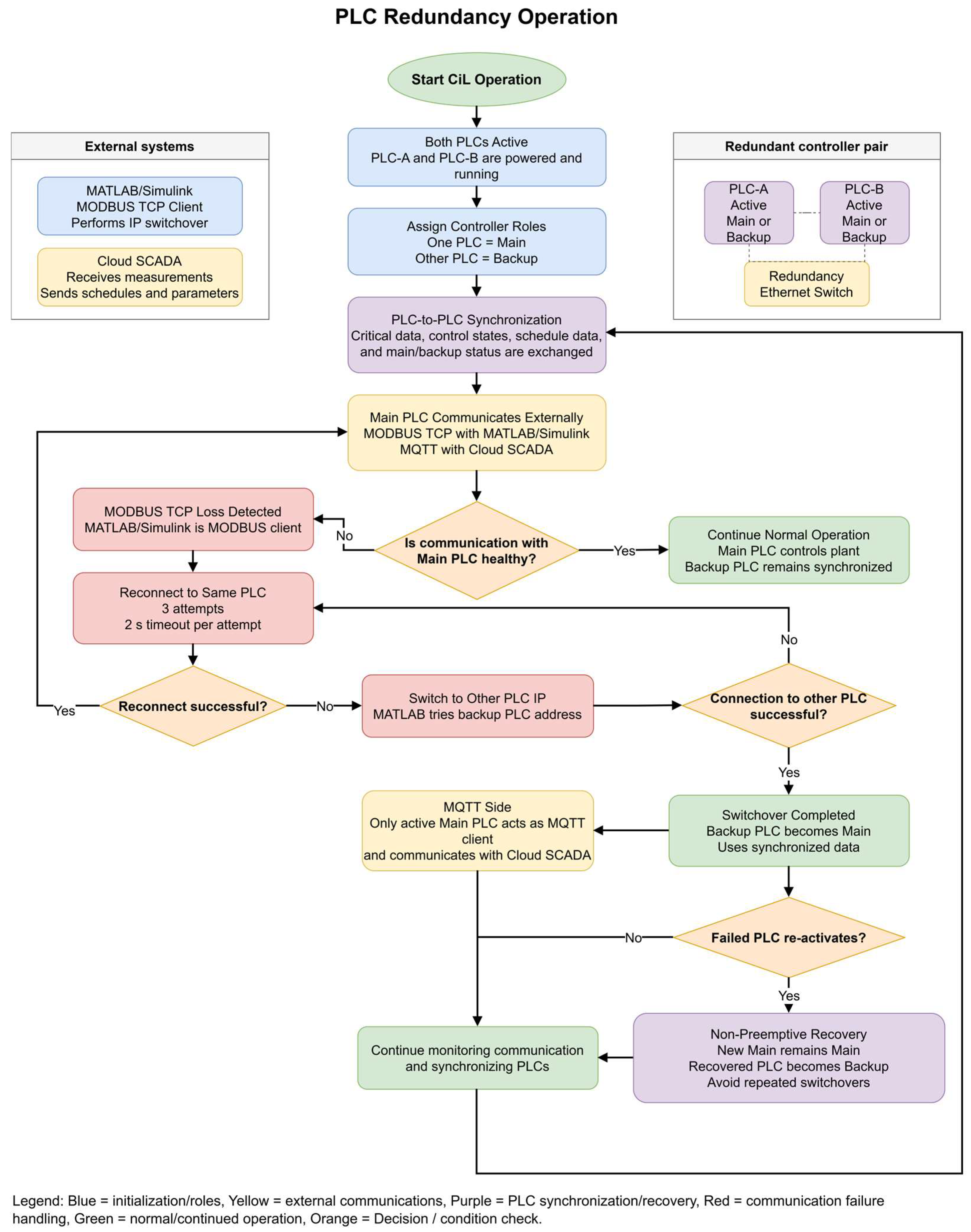
The PPC is implemented on an industrial redundant PLC platform. The redundant controller structure consists of two PLCs and a redundant Ethernet switch. Both PLCs remain active during operation; however, only one PLC operates as the main controller while the other operates as the backup controller. The main PLC is responsible for external communication with the MATLAB/Simulink simulation model and the cloud SCADA system, while the backup PLC remains synchronized and ready to take over in case of a failure.
The two controllers are Phoenix Contact AXC F 3152 PLCnext devices (Phoenix Contact GmbH & Co. KG, Blomberg, Germany). The application is implemented in Structured Text and Function Block Diagram. The controllers use hardware revision 03 and firmware version 2024.0.6, while the engineering software is version 2025.6.
The PLC receives plant measurements from the simulation model and executes the PPC logic cyclically. Based on PoC measurements, plant availability, selected control modes, local limits, and supervisory commands received from SCADA, the PLC calculates the required references for the PV, wind, and BESS subsystems. The active power control layer coordinates renewable curtailment and BESS charging or discharging to satisfy the plant-level active power objective. The reactive power control layer generates the plant-level reactive power reference according to the selected reactive power function, such as constant reactive power control, voltage regulation, or constant power factor control.
The PPC and redundancy programs are assigned to one processor core, while communication tasks are assigned to the other. The PPC task has a configured execution period of 100 ms, and the communication tasks have a configured execution period of 10 ms. These configured task periods are distinct from the MATLAB communication callback spacing and do not represent measured execution or communication latency. On the control core, the redundancy programs have the highest execution priority, followed by the PPC algorithm. All communication programs on the other core have equal execution priority.
The redundancy logic is designed so that only the active main PLC communicates with the external systems. On the MODBUS TCP side, the MATLAB/Simulink model acts as the MODBUS client. Therefore, the IP switchover mechanism is implemented in MATLAB. If communication with the currently connected PLC is lost, MATLAB attempts to reconnect three times, with a timeout of 2 s for each attempt. If all three attempts fail, MATLAB switches to the IP address of the other PLC and attempts to establish communication with it. If this attempt is also unsuccessful, the reconnection process continues alternately until communication with one of the PLCs is restored.
On the SCADA side, MQTT communication is handled by the PLC. Since the PLC acts as the MQTT client, only the active main PLC establishes communication with the cloud SCADA. The SCADA receives measurements from the main PLC and sends the daily function operation schedule and supervisory control parameters to it. The PLC also executes the time-compression algorithm used during accelerated daily profile tests and selects the corresponding scheduled values according to the compressed simulation time.
The two PLCs communicate with each other for critical data synchronization and status exchange. This internal communication is used to keep both controllers updated regarding operating states, control parameters, schedule data, and the current main/backup status. If the main PLC fails, the backup PLC assumes the main role and continues operation using the synchronized data. After a switchover, the newly active PLC remains the main controller even if the failed PLC returns to service. This non-preemptive recovery strategy avoids unnecessary repeated switchovers and improves the stability of the redundant control system. Figure 2 summarizes the main/backup PLC logic, the MATLAB-side MODBUS TCP reconnection sequence, MQTT communication through the active main PLC, data synchronization between redundant controllers, and the non-preemptive recovery strategy used after a PLC switchover.
2.4. Communication and SCADA Infrastructure
Communication architecture is an essential part of CiL validation because the test environment should reproduce not only the control algorithms but also the information-exchange paths used during field operation. In PPC applications, plant measurements, control references, status information, and supervisory commands are exchanged through industrial communication interfaces with different timing and interoperability requirements. MODBUS TCP is suitable for cyclic register-based client–server signal exchange between controllers, field devices, and simulation systems, whereas MQTT provides a lightweight publish–subscribe structure suitable for remote monitoring, cloud integration, and supervisory control [20,22,28]. Other protocols, such as IEC 61850, are also commonly used for industrial interoperability and standardized power-system automation, particularly when formal information models and device-level interoperability are required [29,30]. Accordingly, the proposed CiL platform separates the fast closed-loop plant-control communication from the supervisory SCADA communication.
The first communication layer is the interface between the MATLAB/Simulink model and the PLC-based PPC. This interface is implemented using MODBUS TCP because the exchanged measurements and control commands are represented as cyclic register-based signals. Through this link, the simulation model sends plant measurements to the PLC, and the PLC returns the calculated control commands to the simulation model. This layer therefore represents the plant-to-controller communication path used for PPC validation.
The Modbus TCP interface exchanges 25 signals across 50 16-bit holding registers using Unit ID 1. Each signal is encoded as a 32-bit signed integer with a scaling factor of 1000; the engineering value is multiplied by 1000 before transmission and recovered by dividing the received integer by 1000. MATLAB/Simulink writes 14 signals to the PLC, including plant measurements, BESS availability information, simulation time, and a heartbeat, and reads 11 signals containing controller setpoints and feedback values. The transmitted and received signals occupy holding-register addresses 1–28 and 101–122, respectively, using the address convention in the MATLAB interface.
The interface uses big-endian encoding with the most significant 16-bit word transmitted first and no byte or word swapping. Communication is initiated by a MATLAB timer configured in fixed-spacing mode with a period of 100 ms. This setting specifies the interval between completion of one communication callback and initiation of the next. Each callback reads the controller signals and writes the applicable simulation signals, with most measurement writes performed only when their values change. The Modbus transaction timeout is 2 s.
Figure 2.
PLC redundancy operation scheme.
The second communication layer is the supervisory interface between the cloud SCADA and the PLC. This interface is implemented using MQTT because its publish–subscribe architecture is suitable for remote monitoring, parameter transfer, and schedule-based supervisory operation. The SCADA does not communicate directly with the MATLAB/Simulink model; instead, all supervisory data exchange is performed through the PLC. The SCADA receives plant measurements from the PLC for monitoring and sends the daily operation schedule and operating parameters to the controller.
The scheduled parameters sent by SCADA include the PoC active power upper limit, the BESS open-loop active power setpoint, the minimum SoC limit, and the maximum SoC limit. Each parameter is transmitted as 96 separate values, corresponding to the 96 fifteen-minute intervals of a 24 h day. By storing the full daily schedule locally in the PLC, the controller can continue applying valid scheduled values even if a temporary communication loss occurs between the cloud SCADA and the PLC. This structure reduces dependence on continuous cloud connectivity and improves the robustness of schedule-based operation.
2.5. Time-Compression and Daily Schedule Handling
To accelerate the validation of daily operating scenarios, the PLC implements a time-compression algorithm that maps a complete 24 h operating day into a 240 s CiL simulation window. The time-compression factor, denoted by , is defined as the ratio between the real duration of one day and the duration of the compressed simulation test as in (1).
where is the number of seconds in one day and 240 is the total duration of the accelerated CiL test in seconds. Therefore, 1 s of simulation time represents 360 s, or 6 min, of real daily operation. The flow chart in Figure 3 shows how the PLC converts the selected simulation date into epoch time, compresses a 24 h operating day into a 240 s test, reconstructs hour and minute values from the simulation epoch timestamp, selects the active 15 min schedule index, and publishes time-consistent MQTT data to SCADA.
Figure 3.
Time compression and daily schedule handling algorithm.
The full-day operational profile is reproduced over 240 s of simulation time using a fixed-step configuration with automatic solver selection and a step size of 50 µs. The original production data are sampled at 30 s intervals. With the applied time-compression factor of 360, successive available-power values are supplied to the asset models approximately every 0.08333 s of simulation time and held constant until the next update. The 240 s duration refers to the simulation time axis, rather than a measured wall-clock execution time.
The observed transients characterize the interaction between the industrial PPC and the simplified plant models under accelerated profile replay. The simplified inverter, wind-generation, and BESS converter models respond to setpoint changes more rapidly than the corresponding physical equipment. The simulation step size specifies the numerical integration interval; it does not establish equivalence between simulated and physical equipment dynamics. Accordingly, the accelerated tests evaluate PPC logic implementation, including resource allocation, operating constraints, mode transitions, and schedule execution, rather than physical asset settling times or dynamic equivalence with an uncompressed plant model.
Time compression is applied to the production profiles and supervisory schedule, while the complete BESS SoC integration rate is scaled to represent the corresponding storage-energy evolution. The physical PLC task periods and communication settings remain unchanged. The tests therefore evaluate the implemented logic within the stated CiL configuration without claiming uniformly scaled closed-loop dynamics. Simulation-to-wall-clock timing was not characterized, and the reported simulation-axis response times are not used to demonstrate compliance with physical response-time requirements.
This approach provides a low-cost, functionally comprehensive environment for checking industrial PPC logic before commissioning. It enables daily operating sequences to be examined without requiring a dedicated real-time simulator or a continuous 24 h real-time test, which can be impractical in resource-constrained laboratory setups. The platform therefore supports logic verification and identification of implementation errors, while detailed equipment-dynamic validation and verification of physical response-time requirements remain separate testing objectives.
The SCADA schedule is divided into 96 intervals, where each interval corresponds to 15 min of the 24 h day. The duration of one 15 min schedule interval in compressed simulation time, denoted by , is calculated as in (2).
where s is the real duration of one schedule interval.
The selected simulation date, defined by the year, month, day, and coordinated universal time (UTC) offset, is converted in the PLC to a base Unix epoch timestamp, , using a standard Gregorian calendar conversion. This timestamp represents the beginning of the selected simulated day and is used as the reference time for the compressed daily profile.
The elapsed simulation time, , is then converted into the corresponding timestamp within the compressed 24 h day. The current simulation epoch time, , is calculated using the base timestamp and the compression factor.
where is in milliseconds. Since , the timestamp advances by 360,000 ms for every 1 s increase in simulation time. The PLC inserts into the MQTT messages sent to SCADA, allowing the 240 s CiL test data to be represented as measurements belonging to the selected 24 h calendar day.
The same compressed epoch timestamp is also used to determine the active SCADA schedule interval. After is calculated, the PLC converts this epoch value back into local date-time variables. The reconstructed hour and minute values are then used to select the active 15-min schedule interval.
Since one day is divided into 96 intervals of 15 min, each hour contains four schedule intervals. Therefore, the active schedule index is calculated as in (4).
where is the selected schedule index, is the reconstructed hour, and is the reconstructed minute obtained from the epoch-to-date-time conversion. The index is limited to the range 0–95. If the PLC array uses one-based indexing, the corresponding array index is obtained by adding one to .
The PLC then selects the effective scheduled values using this index. The selected PoC active power upper limit, BESS open-loop active power setpoint, minimum SoC limit, and maximum SoC limit are applied as in (5)–(8).
where , , , and are the effective values used by the PPC at the current simulation instant. This ensures that the scheduled values are selected according to the reconstructed daily time represented by the compressed epoch timestamp. The UTC offset and leap-year logic are considered internally during the epoch-to-date conversion so that the reconstructed hour and minute remain consistent with the selected simulation day.
By storing the full 96-point daily schedule locally in the PLC, the controller does not require a new SCADA command at every control cycle. Instead, the compressed timestamp is used to select the appropriate scheduled values and to publish time-consistent MQTT data. This enables a complete 24 h operating scenario to be validated within a 240 s laboratory test while preserving SCADA schedule consistency and reducing the effect of temporary communication loss between the cloud SCADA and the PLC.
2.6. Integrated CiL Test Operation
During a CiL test, the MATLAB/Simulink model emulates the hybrid power plant and continuously updates the PoC and subsystem measurements. These signals are transmitted to the PLC through MODBUS TCP. The PLC executes the PPC algorithm using the received measurements, the selected control function, and the locally stored SCADA schedule. The resulting setpoints are sent back to the simulation model and applied to the PV, wind, BESS, and reactive power control blocks.
In parallel, the PLC exchanges monitoring and supervisory data with the cloud SCADA through MQTT. This architecture separates the fast plant-control loop from the supervisory scheduling layer: MODBUS TCP is used for real-time interaction between the simulated plant and the PPC, while MQTT is used for SCADA monitoring and daily schedule transfer. Since the actual PLC hardware, communication interfaces, schedule handling, and PPC algorithms are included in the loop, the proposed CiL setup provides a practical pre-commissioning validation environment for the hybrid power plant controller.
2.7. Physical CiL Laboratory Setup
Figure 4 shows the physical laboratory setup used for the CiL validation tests. The setup includes the redundant PLC-based PPC, the simulation computer, Ethernet switches, power supply units, uninterruptible power supply (UPS) equipment, remote I/O modules, and remote terminal unit (RTU) hardware. In the scope of this work, the main components used in the CiL tests are the two PLCs, the Ethernet communication infrastructure, and the PC used for the MATLAB/Simulink hybrid plant simulation. The remaining devices are part of the extended laboratory panel and are available for future integration with field I/O, RTU-based communication, or additional automation tests.
Figure 4.
Physical CiL laboratory setup including redundant PLCs, simulation PC, Ethernet switches, auxiliary power supply, UPS, RTU, and remote I/O modules.
The two PLCs operate as a redundant PPC pair, where one PLC acts as the active main controller and the other remains synchronized as the backup controller. The simulation PC executes the hybrid power plant model and exchanges real-time measurements and control commands with the active PLC through the Ethernet network using MODBUS TCP. The Ethernet switches provide the communication path between the simulation PC, PLCs, and other panel devices. The power supply and UPS system ensure stable auxiliary power for the controller hardware during testing. This physical setup allows the actual controller hardware, redundancy logic, and communication interfaces to be evaluated in closed loop with the simulated hybrid power plant model. The user interfaces used to configure the PPC functions, operate the simulation, and manage Modbus communication are presented in Appendix B.
3. PPC Control Functions
This section describes the eight PPC functions validated in the proposed CiL platform: active power limiting, ramp-rate control, FSM, LFSM-O, LFSM-U, voltage control, constant power factor control, and constant reactive power control. The PPC operates as a closed-loop plant controller: it receives real-time PoC measurements, compares them with the selected references or limits, and generates active and reactive power commands for the PV, wind, and BESS subsystems. The active power controller is responsible for power limitation, ramp-rate control, and frequency support, while the reactive power controller provides constant Q, constant power factor, and voltage-control operation.
The evaluated control functions are based on the European Network of Transmission System Operators for Electricity (ENTSO-E) Requirements for Generators grid code [3], while the voltage-to-reactive-power characteristic follows Annex 18 of the Turkish grid code [31]. Peak shaving, capacity firming, and BESS open-loop operation are evaluated as plant dispatch functions. The tests focus on implementing and verifying grid support functions within the CiL platform.
The main measured variables are the active power , reactive power , voltage , and frequency at the point of connection. The nominal system frequency is denoted by , where Hz. The saturation function used throughout this section is defined as in (9).
where is the input value, is the lower limit, and is the upper limit.
3.1. Active Power Control Structure
The active power control system operates in a closed loop based on the measured active power at the PoC. The selected active power reference is compared with the measured active power , and the error is processed by a proportional–integral (PI) controller as in (10) and (11) respectively.
where is the active power error, is the active power PI controller output, is the proportional gain, and is the integral gain. The controller output is limited by the available operating range of the plant and dispatched to the PV, wind, and BESS subsystems. Figure 5 presents the block diagram of the active power controller, which separates the active power controller into reference generation, closed-loop power control, and dispatch stages. It shows active power limiting, frequency-support correction, ramp-rate handling, PI control based on PoC active power feedback, and dispatch of plant-level commands to PV, wind, and BESS assets.
Figure 5.
Active power controller block diagram.
3.2. Active Power Limiting Function
Active power limiting is a fundamental PPC function used to ensure that the active power transferred at the PoC does not exceed connection-agreement, grid-operator, plant-operator, or scheduled limits. In hybrid plants, this function may coordinate renewable curtailment with BESS charging or discharging depending on the selected operating mode and available plant capability. The active power limiting function ensures that the measured active power at the PoC remains below the permitted upper limit. The limit can originate from the connection agreement, grid operator, plant operator, or SCADA daily schedule. The effective active power limit is selected as in (12).
where is the connection agreement limit, is the grid-operator limit, is the plant-operator limit, and is the scheduled active power upper limit received from SCADA.
In active power limiting mode, the active power reference is set according to the selected limit as in (13).
The closed-loop active power error is therefore as given in (14).
where is the active power limiting error. If exceeds , the error becomes negative, and the PI controller reduces the plant active power command. In the hybrid plant, this reduction is achieved by increasing BESS charging when SoC allows it and/or by curtailing PV and wind generation. If is below the limit, the controller allows the plant output to increase within the available renewable power, BESS constraints, and ramp-rate limits. Thus, active power limitation is performed as a measurement-based closed-loop control function rather than a feedforward calculation.
Active power limiting control can be operated by one of the three methods below:
- Peak-shaving mode: When peak-shaving is enabled, the PPC limits active power at the PoC primarily by charging the BESS (absorbing excess power). If charging the BESS is not sufficient to meet the PoC limit, the PPC then curtails the production units. Priority: charge the BESS first, curtail generation second.
- Capacity-firming mode: Capacity-firming aims to keep the PoC active power at the requested setpoint using all available resources. If generation is below the setpoint, the PPC discharges the BESS to increase PoC power. If generation is above the setpoint, the PPC charges the BESS to reduce PoC power to the setpoint.
- BESS open-loop mode: In the open-loop mode, the BESS is controlled manually and directly (outside the PPC). The PPC still maintains the PoC active power limit by curtailing production units when needed. If PoC power exceeds the limit, production units will be curtailed even if the BESS is discharging.
Figure 6 illustrates how the PPC selects between peak-shaving, capacity-firming, and BESS open-loop modes, including the use of hysteresis logic to avoid repeated mode changes and the priority of BESS charging/discharging or renewable curtailment depending on the selected mode.
Figure 6.
Active power limiting operation mode activation algorithm.
3.3. Ramp-Rate Control Function
The ramp-rate control function limits how quickly the active power reference is allowed to change. This prevents sudden changes in plant output when the active power limit or SCADA schedule changes. Ramp-rate control is not applied to references calculated by the frequency-support functions. This function is used to adjust active power gradually according to the maximum allowable rate of change. Grid codes and connection agreements may restrict the rate at which plant active power is allowed to change. Ramp-rate control converts abrupt changes in operator or SCADA commands into gradual active power trajectories, thereby reducing sudden power variations at the PoC. Frequency-support commands are excluded from this limitation because they require faster response.
Let be the requested active power command at the current PLC cycle , and let be the ramp-limited reference from the previous cycle. The ramp-limited reference is calculated as in (15).
where is the updated ramp-limited reference, is the upward ramp-rate limit, is the downward ramp-rate limit, and is the PLC control-cycle time. If ramp-rate control is disabled, the requested command is applied directly.
3.4. Frequency-Support Functions
Grid codes and TSO requirements define frequency-dependent active power response characteristics for renewable power plants, including droop-based frequency support and limited frequency-sensitive operation [3]. In this study, three frequency-support functions are implemented and validated: FSM, LFSM-O, and LFSM-U.
Previous studies have investigated active-power-based frequency support, synthetic inertia, virtual inertia, and coordinated PV–wind–BESS frequency regulation for converter-interfaced renewable plants [32,33,34,35]. These studies demonstrate the importance of validating frequency-support behavior in low-inertia systems. However, the experimental scope of this paper focuses on droop-based FSM, LFSM-O, and LFSM-U functions implemented in the industrial PPC.
FSM provides a proportional active power response to frequency deviations in both under-frequency and over-frequency regions. LFSM-O is activated when the measured frequency exceeds a specified threshold and reduces plant active power to limit further frequency increase. LFSM-U is activated below an under-frequency threshold and increases plant active power when sufficient renewable reserve or BESS discharge capability is available.
In the implemented PPC, LFSM-O and LFSM-U operate according to their respective activation thresholds when FSM is disabled. When FSM is enabled, it has priority over the limited frequency-sensitive modes. Ramp-rate limitation is not applied to these references because frequency-support functions require rapid active power response. This priority is configurable via the controller’s user interface.
The general droop constant for frequency response is as in (16).
where is the active power-frequency gain, is the nominal active power of the plant, is the droop setting in percent, and is the nominal frequency.
In FSM, the PPC responds to both under-frequency and over-frequency deviations. The active power correction is as in (17).
where and are the under-frequency and over-frequency activation thresholds, and are the corresponding droop gains, and and are the maximum allowed active power increase and reduction.
LFSM-U is activated only when the frequency falls below its under-frequency threshold as in (18).
where is the LFSM-U activation threshold and is the maximum allowed increase in active power. This function increases the active power reference when sufficient reserve or BESS discharge capability is available. Figure 7 demonstrates the priority logic among FSM, LFSM-U, and LFSM-O. FSM overrides the limited frequency-sensitive modes when enabled, while LFSM-U and LFSM-O operate according to their under-frequency and over-frequency thresholds when FSM is not active.
Figure 7.
Frequency-support reference selection algorithm.
LFSM-O is activated only when the frequency exceeds its over-frequency threshold as in (19).
where is the LFSM-O activation threshold and is the maximum allowed active power reduction. This reduction is achieved through BESS charging and/or renewable curtailment.
The active power reference after frequency support is as in (20).
where is the active power reference before frequency correction, and is the active power correction from FSM, LFSM-U, or LFSM-O. The resulting reference is limited by plant capability and sent directly to the active power PI controller, since ramp-rate limitation is not applied to frequency-support references.
3.5. Reactive Power Control Structure
Renewable power plant PPCs commonly provide several reactive power control modes. Constant reactive power control maintains a specified reactive power exchange at the PoC. Constant power factor control calculates the required reactive power according to the measured active power and requested power factor. Voltage control adjusts the reactive power reference according to the deviation between the measured and requested PoC voltage while respecting the available reactive power capability of the plant. Only one reactive power control mode is active at a time. The reactive power control system also operates in closed loop using the measured reactive power at the PoC. The selected reactive power reference is compared with the measured reactive power as in (21), and the error is used in the PI controller as in (22).
where is the reactive power error, is the reactive power PI controller output, is the proportional gain, and is the integral gain. The calculated output is limited according to the reactive power capability of the plant. In this paper, positive reactive power corresponds to capacitive operation, while negative reactive power corresponds to inductive operation. Figure 8 demonstrates the reactive power reference-generation modes, including constant Q, voltage control, and constant power factor control, followed by closed-loop reactive power PI control and dispatch of the resulting reactive power command to the available plant assets.
Figure 8.
Reactive power controller block diagram.
3.6. Constant Reactive Power Control
In constant reactive power mode, the PPC tracks a fixed reactive power setpoint received from the operator or SCADA. The reference is as in (23).
where is the requested reactive power value. This reference is limited by the available reactive power capability of the plant before being applied to the reactive power PI controller. The controller then adjusts the plant reactive power command until the measured tracks the selected setpoint.
3.7. Constant Power Factor Control
In constant power factor mode, the PPC converts the requested power factor into an equivalent reactive power reference. Let be the requested power factor magnitude. The corresponding power factor angle is as in (24).
The reactive power reference is then calculated as in (25).
where is the reactive power reference, is the measured active power at the PoC, and defines the operating direction. In the adopted sign convention, represents capacitive operation and represents inductive operation. The calculated reference is limited by the available reactive power capability before being sent to the reactive power PI controller.
3.8. Voltage Control Function
The voltage control function regulates the PoC voltage by generating a reactive power reference according to the measured voltage deviation and the available PQ capability of the plant. The implementation consists of two main parts: calculation of the available reactive power capability , and calculation of the voltage-control reactive power reference .
- (1)
- Qmax Calculation
The available reactive power capability is calculated according to the real-time measured active power production and the plant PQ capability curve. The curve is represented by active power breakpoints and corresponding reactive power capability values. For an operating point between two breakpoints, and , the available reactive power capability is obtained by linear interpolation as in (26).
where and are the reactive power capability values at the two neighboring active power breakpoints. This interpolation is applied to calculate the magnitude of the maximum reactive power and is used for both inductive and capacitive sides of the PQ capability curve.
- (2)
- Qref Calculation
The voltage deviation is calculated using the measured PoC voltage as in (27).
where is the voltage deviation in per unit, is the measured PoC voltage, is the voltage reference, and is the nominal voltage at the connection point.
The voltage droop in per unit is as in (28).
where is the voltage droop setting in percent. The voltage-control reactive power reference is calculated as in (29).
Thus, when the measured PoC voltage is lower than the voltage reference, , and the PPC generates a positive capacitive reactive power reference. When the measured PoC voltage is higher than the voltage reference, , and the PPC generates a negative inductive reactive power reference. The resulting is limited by the available PQ capability and then tracked by the reactive power PI controller.
3.9. Final Reference Selection
The final active-power reference is selected from the applicable plant limit and frequency-support function according to the implemented mode priority. Ramp-rate limitation is applied to ordinary active-power commands when enabled, while frequency-support references bypass the ramp limiter. The selected reference is tracked by the closed-loop active-power PI controller using the measured PoC active power.
For reactive power, only one mode is active at a time. The selected reference is defined in (30).
where is the constant reactive power setpoint, is the power-factor-based reactive power reference, and is the voltage-control reference. The selected reactive power reference is tracked by the closed-loop reactive power PI controller using the measured .
3.10. Controller Parameterization
The active- and reactive-power PI controllers were tuned empirically by trial and error using the responses of the simulated plant. The active-power PI controller uses a proportional gain of and an integral gain of , while the reactive-power PI controller uses and . These values are reported as configured in the PLC implementation, whose PPC task period is 100 ms. Table 2 summarizes the controller output limits and operating-mode settings used in the tests.
Table 2.
Controller operating parameters and settings.
The ramp-rate setting is implemented in the physical PLC control task described in Section 2.3. Its configured value and the response plotted on the simulation time axis represent different time bases. Because their timing relationship was not characterized, the plotted trajectory is used to assess ramp-rate function operation within the CiL configuration rather than to verify a physical plant ramp rate.
4. Experimental Validation Results
4.1. Quantitative Evaluation Procedure
The quantitative assessment considers mean absolute error (MAE), maximum error (), normalized tracking accuracy (), steady-state error (SSE), directional overshoot (OS), and settling time (). These metrics characterize average tracking performance, the largest deviation, residual error after the response stabilizes, excursion beyond the target, and the time required to reach the specified tolerance.
A common initialization interval of 0–1.5 s is excluded from all evaluated modes, including redundancy. Analysis is restricted to the remaining samples within each figure’s displayed time interval. Reference changes initiated before 1.5 s are excluded from the dynamic assessment, while the preceding reference history is retained to identify ramps already in progress. Full-day profiles characterize the input data and are excluded from the function comparison in Table 3. Redundancy is evaluated separately.
Table 3.
Tracking and dynamic-response metrics for the evaluated control modes after exclusion of the initialization interval.
Let denote the plant active or reactive power reference and the corresponding PoC measurement at sample . The signed tracking error is defined in (31).
For active power upper-limit modes, the evaluation error includes only positive deviations, as defined in (32) since the controller’s objective is to prevent exceeding the limit and not achieve the setpoint in these modes. During intentional downward-reference response windows, the absolute-error definition in (33) is used instead. Capacity firming and all reactive power modes are evaluated using (33).
A downward-reference response window ends immediately before the next reference change or 2.0 s after the step or ramp finishes, whichever occurs first.
The MAE represents the time-weighted average evaluation error and is calculated using (34), where N is the number of retained samples, and ti is the timestamp of sample i.
identifies the largest evaluation error, while normalized tracking accuracy, , expresses the average error relative to a common power base. Both are calculated using (35), where B is the applicable normalization base.
The normalization bases are 172.2 MW for active power and 55.608 MVAr for reactive power. The reactive power base is the largest absolute reference in the selected reactive test intervals and represents a common test scale rather than nameplate capability.
For capacity firming only, the maximum error reported in Table 3 uses the upper-side statistic defined in (36) instead of the maximum-error expression in (35), capped for reporting at 10 MW to correspond to the nominal BESS active-power rating.
This statistic does not represent the maximum absolute mismatch or quantify below-reference deviations. MAE, accuracy, and the dynamic metrics continue to use uncapped data.
Reference steps are identified by changes of at least 0.5 MW or MVAr. For ramp-rate evaluation, successive same-direction increments exceeding 10−6 MW are grouped when their separation does not exceed 0.150 s, provided the total reference change is at least 0.5 MW. Dynamic assessment considers downward reference changes in active power upper-limit modes and both directions in capacity-firming and reactive power modes.
Let denote the start of a reference change, the end of the step or ramp, and the observation-window end. The window ends immediately before the next reference change or no later than 2.0 s after tb. The settling tolerance is calculated using (37), where is the signed change from the pre-change reference to the final step or ramp reference.
The minimum tolerance is 0.1 MW for active power and 0.1 MVAr for reactive power. The settling instant is the earliest recorded instant at or after from which the absolute tracking error remains within this tolerance through , with at least 0.1 s of continuous in-band observation. Settling time and post-ramp settling time are calculated using (38).
Table 3 reports the largest available settling-time value satisfying this criterion. Values that cannot be established within the observation window are omitted. For ramp-rate control, the reported settling time includes the ramp duration.
SSE characterizes the residual tracking error after the response has stabilized. It is evaluated over the final portion of each response window, with the terminal averaging duration L defined in (39).
Let J denote the set of indices i for which the sample interval lies entirely within . The time-weighted terminal mean absolute error is calculated using (40).
An SSE value is included only when the entire terminal interval follows the identified settling instant.
Directional overshoot is calculated using (41). It measures the excursion beyond the reference in the direction of the commanded change, including below-reference excursions following a reduction. The sign function distinguishes upward and downward changes.
Percentage overshoot is calculated using (42) and is defined only for nonzero reference changes.
Controller redundancy is evaluated using two complementary metrics: peak deviation, , which measures the largest absolute reference-to-measurement difference following a PLC role transfer, and PoC output recovery time, , which measures the time required for the controlled output to return to and remain within a specified tolerance.
For each recorded Active PLC transition at , the observation window extends up to 2.0 s and ends one sample before the next transition if this occurs earlier. The recovery tolerances are ±1.722 MW for active power and ±0.55608 MVAr for reactive power, corresponding to 1% of the respective normalization bases. The recovery instant is the earliest recorded instant from which the absolute tracking error remains within the applicable tolerance through the window end, with at least 0.1 s of continuous in-band observation. Output recovery time and peak deviation are calculated using (43).
If the output remains within the tolerance throughout the observation window and satisfies the minimum observation duration, the recovery time is zero. A recovery time is not assigned when the final in-band requirement cannot be established. The recorded sample interval is 0.005 s. These metrics describe output recovery on the simulation time axis; they do not measure fault-detection latency, command interruption, or wall-clock network failover. The recorded PLC role changes identify the assessment starting points rather than independently verified fault-inception times.
4.2. Full-Day Profile Validation
Two full-day active power profiles were used to evaluate the PPC behavior under realistic daily renewable production conditions. The profiles belong to two different operating days and therefore include different renewable production characteristics. The first profile is more suitable for evaluating peak-shaving and frequency-support operation, while the second profile is more suitable for evaluating capacity-firming behavior. Both full-day profile simulations were run using the default active power operation mode, namely peak-shaving mode, with the plant active power limit set to 1 pu.
The full-day plots are used primarily to demonstrate the operational data profiles and their variability. Both displayed cases operate in peak-shaving mode. They are not included in the function-by-function quantitative comparison in Table 3.
Figure 9 shows the first full-day profile under normal operation, including the interaction between peak-shaving control, BESS charging, and renewable curtailment. At T1, the measured PoC active power reaches the plant active power upper limit while the BESS is still available for charging. Therefore, the PPC activates peak-shaving operation by charging the BESS. This is observed in the asset production subplot as the BESS power moves in the negative direction, while the SoC begins to increase. At T2, the available renewable production falls below the active power limit. Since peak-shaving is no longer required, the PPC stops charging the BESS, and the SoC remains constant. During the following interval, the PoC active power follows the available renewable production and remains below the limit without requiring additional limiting action. At T3, the PoC active power again approaches the active power upper limit. As the BESS still has remaining charging capacity, the PPC reactivates peak-shaving by charging the BESS. This results in a rapid increase in SoC while the measured PoC active power is maintained close to the plant limit. At T4, the BESS reaches its maximum SoC limit and can no longer absorb excess renewable production. Consequently, the PPC automatically switches from BESS charging to renewable curtailment. This behavior is visible in the asset production subplot, where the wind power output is curtailed after the BESS becomes fully charged. From this point until the end of the simulated day, the controller maintains the PoC active power at the prescribed upper limit primarily through WPP curtailment. Overall, the profile demonstrates a complete full-day simulation of normal operation, where the PPC first uses BESS charging for peak-shaving when storage capacity is available and then automatically applies renewable curtailment after the BESS reaches its maximum SoC.
Figure 9.
Full-day profile curve under the normal operating mode used for peak-shaving and frequency-support function tests.
Figure 10 shows the second full-day production profile under the default peak-shaving operating mode. Although this profile contains stronger renewable production fluctuations and is therefore more suitable for capacity-firming validation, it is first operated in peak-shaving mode to observe the daily plant behavior under normal operating conditions. At T1, the measured PoC active power reaches the plant active power upper limit while the BESS is available for charging. Therefore, the PPC activates peak-shaving operation by charging the BESS. This is observed in the asset production subplot as the BESS power moves in the negative direction, while the SoC begins to increase. At T2, the available renewable production decreases below the active power limit. Since no limiting action is required, the PPC stops charging the BESS, and the SoC remains constant. During this interval, the PoC active power follows the available renewable production without additional peak-shaving action. At T3, the PoC active power again reaches the active power upper limit. Since the BESS still has available charging capacity, the PPC reactivates peak-shaving by charging the BESS. As a result, the SoC increases rapidly while the PoC active power is maintained close to the plant limit. At T4, the BESS reaches its maximum SoC limit and can no longer absorb excess renewable generation. Consequently, the PPC automatically switches from BESS charging to renewable curtailment. This behavior is visible in the asset production subplot, where the WPP output is limited while the PoC active power remains at the prescribed upper limit. Between T4 and T5, the controller continues to maintain the PoC active power limit primarily through WPP curtailment. After T5, the available renewable production falls below the limit, so curtailment is no longer required. The PoC active power then follows the available production again.
Figure 10.
Full-day production curve used for capacity-firming testing.
4.3. Active Power Limiting and Ramp-Rate Control Validation
The active power limiting function was validated in the three operating modes described in Section 3: peak-shaving mode, capacity-firming mode, and BESS open-loop mode. For these three tests, ramp-rate control was disabled so that the active power limiting response of each mode could be evaluated directly. The active power references were changed using 20% increments and decrements based on the 172.2 MW base power. This sequence was selected to verify both downward and upward active power control actions.
First, active power limiting was tested in peak-shaving mode. In this mode, the PPC limits the active power at the PoC primarily by charging the BESS when sufficient charging capacity is available; otherwise, renewable production is curtailed. As shown in Figure 11, the peak-shaving limit is first reduced in 20% steps and then increased again in 20% steps. At T1, the decreasing reference sequence begins, and the measured PoC active power follows the reduced plant reference. During this interval, the BESS is charged to absorb excess active power, as indicated by the negative BESS power and the increasing SoC. At T2, the measured PoC active power reaches zero, demonstrating that the PPC can reduce the plant output to the minimum operating point during peak-shaving operation. At T3, the reference begins to increase again. Around this point, the BESS reaches its maximum SoC limit; however, the peak-shaving operation continues without interruption, since the controller adjusts renewable production instead of relying on further BESS charging. Finally, at T4, the active power limit reaches 100% of the base value, and the measured PoC active power follows the increasing reference back to the full-limit operating region.
Figure 11.
Active power limiting validation in peak-shaving mode without ramp-rate control under 20% decreasing and increasing reference steps.
Second, active power limiting was tested in capacity-firming mode. In this mode, the PPC aims to regulate the PoC active power around the requested setpoint using all available plant resources. If renewable production is higher than the requested setpoint, the PPC reduces PoC active power by charging the BESS and/or curtailing production. If renewable production is lower than the requested setpoint, the PPC increases PoC active power by discharging the BESS when sufficient energy is available.
As shown in Figure 12, at T1, the available renewable production begins to fluctuate. The PPC responds by charging or discharging the BESS to compensate for these variations and keep the PoC active power close to the selected reference. This behavior is visible in the BESS power and SoC traces, where the BESS changes its operating direction depending on whether the available production is above or below the setpoint. At T2, the BESS reaches its maximum SoC limit and can no longer absorb additional excess production. Therefore, the PPC curtails the WPP to maintain the PoC active power at the requested value. At T3, the active power reference is reduced by 20%, and the measured PoC active power follows the new lower setpoint. At T4, the reference is returned to 50%, and the controller again brings the PoC active power back to the selected operating point. At T5, the reference is increased by 20%. Since the available renewable production is not sufficient to reach the higher setpoint, the PPC first releases curtailment and then discharges the BESS to support the PoC active power. However, the combined available production and BESS contribution are initially still insufficient to fully reach the requested value. At T6, the measured PoC active power reaches the increased setpoint, confirming successful tracking once sufficient power becomes available. Finally, at T7, the reference is reduced back to 50%, and the PPC successfully regulates the PoC active power to the new setpoint.
Figure 12.
Active power limiting validation in capacity-firming mode without ramp-rate control under 20% decreasing and increasing reference steps.
Third, active power limiting was tested in BESS open-loop mode. In this mode, the BESS active power setpoint is applied independently, while the PPC maintains the PoC active power limit by adjusting the renewable production units when necessary. Therefore, the BESS is not used as the main closed-loop active power limiting resource; instead, the PPC compensates for the externally commanded BESS behavior by curtailing or releasing renewable production.
As shown in Figure 13, the simulation starts with the PoC active power limit set to 100% of the base value, while the available production is slightly below this limit. At T1, a manual 10 MW charging command is applied to the BESS. This causes the measured PoC active power to decrease, since part of the renewable production is absorbed by the BESS. The PPC does not apply additional limiting action during this interval because the PoC active power remains below the selected limit. At T2, the BESS charging command is removed, and the measured PoC active power increases slightly until it reaches the active power limit. At T3, the BESS is manually commanded to discharge. Since BESS discharge increases the active power injected toward the PoC, the PPC responds by curtailing the WPP to prevent the PoC active power from exceeding the limit. At T4, the PoC active power limit starts to decrease in 10% steps while the BESS continues discharging. The measured PoC active power follows the reduced limits, demonstrating that the PPC can maintain the PoC limit regardless of the externally imposed BESS operating condition. At T5, the active power limit starts to increase again, and the controller releases curtailment accordingly until the limit reaches 100% at T6. At T7, the BESS reaches its minimum SoC limit and can no longer continue discharging. As a result, the measured PoC active power falls below the 100% limit due to the available renewable production. These results confirm that, even when the BESS is operated independently in open-loop mode, the PPC successfully maintains the PoC active power limit by curtailing or releasing renewable production as needed.
Figure 13.
Active power limiting validation in BESS open-loop mode without ramp-rate control under 10% decreasing and increasing reference steps.
The ramp-rate control function was then validated by applying active power reference changes with ramp-rate control enabled. In this test, the plant active power reference was decreased using 20% steps until it reached zero and was then increased using 20% steps until the requested reference reached 100% of the base value. The purpose of this test was to verify that abrupt active power reference changes are not directly applied to the plant controller, but are converted into ramp-limited active power trajectories.
Figure 14 shows the ramp-rate control validation under decreasing and increasing active power reference changes. At T1, the active power setpoint starts to decrease, and the measured PoC active power follows the ramp-limited reference smoothly instead of responding with abrupt step changes. At T2, the BESS reaches its maximum SoC limit; however, this does not cause a significant disturbance in the measured PoC active power, since the PPC reacts quickly and continues regulating the plant output through renewable production adjustment. At T3, the measured PoC active power reaches zero, confirming that the controller can reduce the plant output to the minimum operating point while respecting the ramp-rate limitation. After T3, the active power reference starts to increase again, and the measured PoC active power follows the ramp-limited trajectory during the upward transition. Around T4, the requested reference exceeds the available renewable production. Therefore, the PoC active power remains below the requested limit.
Figure 14.
Ramp-rate control validation under 20% decreasing and increasing active power reference steps.
4.4. Frequency-Support Function Validation
The frequency-support functions were validated by applying synthetic measured frequency signals to the PPC. This approach allows the under-frequency and over-frequency operating regions to be tested in a controlled and repeatable way without disturbing the rest of the simulated plant model. The synthetic frequency profiles were applied using 0.2 Hz steps. During these tests, the active power response was evaluated by comparing the measured frequency signal, the calculated active power reference, and the measured active power at the PoC. Ramp-rate limitation was not applied to the frequency-support references because these functions must respond rapidly to frequency deviations. The FSM test was performed using a synthetic frequency profile that moves away from the nominal frequency in both directions and then returns to nominal. The synthetic frequency measurement is applied in the controller through a signal-selection logic that disconnects the real frequency measurement and replaces it with a manually adjustable frequency signal entered via the controller’s web human–machine interface (WHMI).
Figure 15 presents the FSM validation using a synthetic frequency signal. To enable active power increase during the under-frequency test, the plant active power limit was first reduced to 50% at T1. At T2, the synthetic frequency signal was decreased in successive 0.2 Hz steps. After the first step, the controller does not react because the measured frequency remains within the configured deadband. As three additional under-frequency steps are applied, the PPC increases the PoC active power accordingly, demonstrating the expected FSM response under under-frequency conditions. At T3, the frequency is returned to its nominal value, and the PoC active power correspondingly returns to the 50% operating limit. At T4, the synthetic frequency is increased in 0.2 Hz steps to test the over-frequency response. Similar to the under-frequency case, the first step does not produce a response because the frequency remains within the deadband. As the subsequent over-frequency steps are applied, the PPC reduces the PoC active power in accordance with the FSM characteristic. Finally, at T5, the frequency is restored to its nominal value, and the PoC active power returns to the pre-disturbance operating point defined by the 50% limit.
Figure 15.
FSM validation using synthetic under-frequency and over-frequency deviations.
The LFSM-O function was tested using a synthetic frequency signal that increases above the over-frequency activation threshold and then returns to nominal frequency. As shown in Figure 16, the synthetic frequency starts to increase in steps at T1. The PPC does not react after the first frequency step because the measured frequency is still below the LFSM-O activation threshold. After the second step, the activation threshold is exceeded, and the controller starts reducing the active power reference. As the frequency continues to increase, the measured PoC active power decreases accordingly, following the selected LFSM-O droop characteristic. At T2, the BESS reaches its maximum SoC limit. However, this does not cause a significant disturbance in the measured PoC active power, since the PPC quickly maintains the requested active power reduction through renewable curtailment. After T2, the synthetic frequency signal is gradually reduced back toward the nominal value. As the frequency decreases, the PPC progressively releases the active power reduction, and the measured PoC active power increases accordingly. At T3, the frequency returns to nominal, and the plant resumes normal operation. These results confirm that LFSM-O activates only when the over-frequency threshold is exceeded, reduces active power according to the frequency deviation, and restores the plant output when the frequency returns to the normal operating range.
Figure 16.
LFSM-O validation using a synthetic over-frequency signal.
The LFSM-U function was tested using a synthetic frequency signal that decreases below the under-frequency activation threshold and then returns to nominal frequency. As shown in Figure 17, the plant active power limit is first reduced to 50% at T1 to provide upward regulation margin, since LFSM-U is expected to increase the active power output during under-frequency conditions. At T2, the first under-frequency step is applied. As the frequency continues to decrease in successive steps, the PPC increases the active power reference according to the LFSM-U characteristic, and the measured PoC active power rises accordingly. After the lowest frequency level is reached, an additional decreasing and increasing frequency step is applied between T3 and T4 to verify that the controller continues to respond correctly to changes in the under-frequency region. At T5, the synthetic frequency starts to return toward the nominal value in steps. As the frequency recovers, the PPC gradually reduces the LFSM-U active power contribution, and the measured PoC active power decreases accordingly. At T6, the frequency reaches the nominal value, and the LFSM-U contribution is fully removed. Finally, at T7, the active power limit is released, and the plant returns to normal operation.
Figure 17.
LFSM-U validation using a synthetic under-frequency signal.
4.5. Constant Reactive Power Control Validation
The constant reactive power control function was validated by applying reactive power reference steps in both capacitive and inductive directions. The reference was changed using 11% step changes to evaluate the tracking performance of the closed-loop reactive power controller over different operating points. The sequence also included a return toward the initial operating point to verify stable recovery after the step changes.
As shown in Figure 18, constant reactive power control is first enabled at T1, after which the PPC brings the measured PoC reactive power to the initial reference of 0 MVAr. The reactive power reference is then increased in 11% steps in the positive direction, corresponding to capacitive operation according to the adopted sign convention. The measured reactive power follows each step and reaches the maximum capacitive test value. After T2, the reference is decreased step by step back toward 0 MVAr. Following T3, negative reactive power steps are applied to test inductive operation, and the measured PoC reactive power tracks the requested values until the maximum inductive test value is reached. After T4, the reference is gradually returned toward 0 MVAr, and at T5, the measured reactive power reaches the zero setpoint again.
Figure 18.
Constant reactive power validation with 11% step changes in capacitive and inductive directions.
4.6. Voltage Control Validation
The voltage control function was tested by applying simulated voltage measurement steps while keeping the voltage reference constant at 1 pu. The synthetic voltage measurement was injected using the same method as the synthetic frequency signal. This test was designed to verify whether the PPC generates the correct reactive power response depending on the direction and magnitude of the voltage deviation. When the measured PoC voltage is below the voltage reference, the PPC should generate a capacitive reactive power reference to support the voltage. When the measured PoC voltage is above the voltage reference, the PPC should generate an inductive reactive power reference to reduce the voltage.
The voltage function calculates a reactive-power reference from the imposed voltage deviation, and this reference is tracked by the closed-loop PoC reactive-power controller. The synthetic voltage input keeps the prescribed deviation independent of the reactive-power response, allowing the Q(V) reference calculation and subsequent tracking to be evaluated. Consequently, this test validates the voltage-dependent reference-generation function and reactive-power tracking, but does not assess the voltage response of the connected network.
As shown in Figure 19, the voltage control function was validated using a synthetic PoC voltage signal, while the voltage setpoint was kept constant. At T1, the synthetic voltage measurement starts to increase above the voltage setpoint, and the PPC responds by driving the measured PoC reactive power in the negative direction, corresponding to inductive operation. The voltage is increased in successive 1% Vnom steps, equivalent to 1.54 kV per step, and the reactive power response becomes more inductive until T2. After T3, the synthetic voltage is reduced step by step back toward nominal value, and the measured PoC reactive power correspondingly returns toward zero, reaching the neutral operating point at T4. At T5, the synthetic voltage is decreased below the setpoint in the same 1% Vnom steps. In response, the PPC drives the measured PoC reactive power in the positive direction, corresponding to capacitive operation, until the maximum test value is reached at T6. After T7, the voltage is increased step by step back toward nominal, and the measured PoC reactive power gradually decreases toward zero, reaching the neutral operating point again at T8. These results confirm that the voltage control mode responds correctly to both over-voltage and under-voltage conditions and adjusts the reactive power exchange in the expected direction according to the voltage deviation.
Figure 19.
Voltage control validation in capacitive and inductive operating regions.
4.7. Constant Power Factor Control Validation
The constant power factor control function was tested separately in lagging and leading regimes. In both tests, the requested power factor was changed using 0.01 setpoint variations and then returned to unity power factor. This test verifies the conversion of the requested power factor into the corresponding reactive power reference and the ability of the PPC to regulate the measured power factor at the PoC.
As shown in Figure 20, the power factor control mode was validated by changing the power factor setpoint away from unity in 0.01 steps starting at T1. In response, the PPC adjusts the plant reactive power output so that the measured power factor follows the requested setpoint. The setpoint is progressively moved toward the lagging region, and at T2, the measured power factor reaches 0.95 lagging. After T3, the setpoint is changed back toward unity in the same 0.01 steps, and the controller correspondingly reduces the reactive power output. Finally, at T4, the measured power factor returns to unity.
Figure 20.
Constant power factor validation in lagging regime with 0.01 setpoint variations.
As shown in Figure 21, the power factor control mode was also validated in the leading region by changing the power factor setpoint away from unity in 0.01 steps starting at T1. In response, the PPC adjusts the plant reactive power output so that the measured power factor follows the requested setpoint. The setpoint is progressively moved toward the leading region, and at T2, the measured power factor reaches 0.95 leading. During this interval, the corresponding PoC reactive power increases in the positive direction, consistent with capacitive operation. After T3, the setpoint is changed back toward unity in the same 0.01 steps, and the controller correspondingly reduces the reactive power output. Finally, at T4, the measured power factor returns to unity.
Figure 21.
Constant power factor validation in leading regime with 0.01 setpoint variations.
Table 3 summarizes the calculated performance metrics for the evaluated active and reactive power modes after the common initialization exclusion. MAE, maximum error, SSE, and overshoot are expressed in MW or MVAr, normalized tracking accuracy in percent, and settling time in simulation seconds. The reported SSE, overshoot, and settling time are the largest applicable values across the assessed reference changes. Maximum error includes transient tracking lag, whereas directional overshoot measures excursion beyond the target.
The results in Table 3 should be interpreted jointly: a high normalized accuracy can coexist with a substantial transient maximum because the accuracy score reflects average error over the evaluation interval. For voltage control, the tabulated errors quantify reactive-power reference tracking under the synthetic voltage input. For power-factor control, they likewise quantify reactive-power tracking rather than a separately calculated power-factor error.
4.8. Controller Redundancy Validation
The redundancy tests comprised two disturbance scenarios. The first two transfers were initiated by de-energizing the active PLC, first PLC 1 and then PLC 2, and subsequently re-energizing each controller before de-energizing the other. The third and fourth transfers were initiated by disconnecting and subsequently reconnecting the active controller’s communication interface. Recovery is measured from the recorded Active PLC transition, rather than from the instant of power removal or communication disconnection. During an unsuccessful Modbus read, the MATLAB communication callback returns without replacing the previously assigned command variables. The simulation therefore retains its last assigned references until a successful read provides updated values. Table 4 presents the recorded transfer times and directions, together with the peak deviations and PoC output recovery times for active and reactive power.
Table 4.
Peak deviations and PoC output recovery times during PLC power-interruption and communication-disconnection tests.
The controller redundancy test was carried out to verify whether the redundant PLC structure can maintain PPC operation during controller switchovers. The validation figures include an additional subplot showing the active PLC number. In this subplot, a value of 1 indicates that PLC1 is the active main controller, while a value of 2 indicates that PLC2 is the active main controller. The test sequence begins with PLC1 as the active controller, switches to PLC2, returns to PLC1, switches again to PLC2, and finally returns to PLC1.
Figure 22 and Figure 23 show the active and reactive power responses during the four recorded PLC role transfers. The controller resumes regulation following the transfers, although the magnitude and duration of the associated output deviations differ between transitions. Table 4 quantifies these deviations and the corresponding PoC output recovery times.
Figure 22.
Controller redundancy validation during active power control with active PLC indication.
Figure 23.
Controller redundancy validation during reactive power control with active PLC indication.
As shown in Table 4, the second transfer produces the largest measured deviations, 35.759 MW and 20.684 MVAr, with active- and reactive-power output recovery times of 1.605 s and 1.395 s, respectively. During the communication-disconnection tests, the third transfer produces peak deviations of 9.967 MW and 0.895 MVAr, with recovery times of 0.35 s and 0.180 s, respectively. The fourth transfer produces peak deviations of 0.182 MW and 1.702 MVAr; active power remains within its recovery tolerance, while reactive power recovers within 0.080 s. Active power also remains within the specified tolerance throughout the first transfer’s observation window. These results characterize the controlled-output response to PLC power interruptions and communication disconnections. The reported recovery times exclude any delay between disturbance initiation and the recorded PLC role change and therefore do not represent total fault-detection or failover times.
5. Discussion
The experimental results demonstrate that the proposed PLC-based CiL platform provides a practical validation environment for industrial PPCs used in utility-scale hybrid PV–wind–BESS power plants. The main advantage of the proposed approach is that the actual industrial PPC hardware is included in the loop. Therefore, the validation covers not only the embedded control algorithms, but also the PLC cyclic execution, communication handling, signal mapping, SCADA interaction, schedule processing, and redundancy logic. This makes the proposed CiL system more representative of field operation than conventional offline simulation, while maintaining the repeatability, safety, and low cost of laboratory testing.
Previous CHIL, HIL, and CiL studies include multifunction validation, although their plant representations, controller hardware, and integration scope differ. The present framework brings coordinated PV–wind–BESS control, industrial PPC redundancy, SCADA schedule handling, and communication testing into a single plant-specific validation environment. In contrast, this work validates an industrial redundant PLC-based PPC responsible for coordinating PV, wind, and BESS subsystems in an actual utility-scale hybrid renewable power plant. This hybrid-plant-specific CiL formulation is a key distinction of the proposed work, since the validation target is not an individual inverter or generic controller, but the plant-level PPC responsible for coordinated operation at the PoC, SCADA schedule handling, industrial communication, redundancy logic, and grid-code-oriented control.
The objectives evaluated here complement the energy-management objectives considered in [21], which addresses power-quality improvement and cost reduction through fuzzy energy management in a hybrid AC/DC microgrid. The present PPC uses deterministic priorities to coordinate renewable curtailment and BESS operation while executing plant-level references and operating constraints. Its evaluation focuses on industrial PLC implementation and the interaction of control logic with communication, scheduling, and redundancy. Operating-cost minimization, battery-degradation minimization, optimal reserve scheduling, and harmonic optimization are outside the implemented control objectives. No quantitative comparison with a fuzzy EMS under matched operating conditions was performed; the comparison therefore distinguishes control objectives and experimental scope rather than establishing the superiority of either approach.
The validation results confirm that the proposed CiL platform can be used to assess the applicability of multiple grid-code-oriented PPC functions within a single integrated environment. The active power tests demonstrated coordinated operation of renewable curtailment and BESS charging/discharging under different operating modes, while the frequency-support and reactive power tests confirmed the expected plant-level response under the selected control characteristics. In addition, the full-day profile tests showed that real operational data can be used in the CiL environment to reproduce realistic renewable variability, BESS coordination, curtailment behavior, and connection-limit enforcement. These results support the use of the proposed CiL method as a pre-commissioning validation step for hybrid renewable power plant controllers.
Another important aspect of the proposed framework is the use of industrial communication protocols that reflect the architecture encountered in commercial renewable power plants. MODBUS TCP is used for cyclic closed-loop signal exchange between the MATLAB/Simulink model and the PLC-based PPC, whereas MQTT is used for SCADA monitoring, supervisory commands, and daily schedule transfer. As a result, the platform validates not only the PPC algorithms, but also the communication and integration structure that can become a major source of commissioning problems in industrial projects. The time-compression strategy further improves the practicality of the framework by allowing complete 24 h operating scenarios to be reproduced within a short laboratory test while preserving the original SCADA schedule logic implemented in the PLC.
The redundant PLC structure is also significant for utility-scale plant operation. PPC availability is directly related to grid-code compliance, connection-limit enforcement, and the ability of the plant to provide required active and reactive power functions. A controller failure or communication interruption may lead to loss of plant-level regulation or non-compliance with operating requirements. By validating the main/backup PLC operation, synchronization, switchover behavior, and non-preemptive recovery in the CiL environment, redundancy-related risks can be evaluated before site deployment. The redundancy tests therefore show that the proposed platform can support not only functional validation, but also reliability-oriented controller verification.
The use of MATLAB/Simulink instead of a dedicated real-time simulation platform is appropriate for the scope of this study because the objective is plant-level PPC validation through signal exchange with the actual PLC, rather than electromagnetic transient simulation or power-hardware interfacing. The investigated PPC functions operate using plant-level measurements such as active power, reactive power, voltage, frequency, SoC, and asset power limits. These dynamics are compatible with the considered simulation environment, and deterministic microsecond-level execution is not required for validating the intended supervisory control functions. Dedicated real-time simulators such as OPAL-RT or RTDS would be more suitable for detailed converter switching studies, protection interaction, sub-cycle electromagnetic transients, PHIL testing, or high-fidelity fault ride-through validation. However, for the plant-level PPC validation addressed in this work, MATLAB/Simulink provides a lower-cost and computationally efficient alternative.
The proposed methodology is also scalable. Since the controller exchanges plant-level measurements and references through standardized industrial communication protocols, additional renewable generation units, storage systems, SCADA schedule variables, or supervisory control functions can be incorporated with limited modifications to the simulation model and communication register structure. This makes the framework suitable for future hybrid renewable power plants with larger numbers of distributed assets and more complex operating strategies.
Future extensions could include controlled tests of partial inverter unavailability, reduced generation capacity, degraded feedback signals, and communication interruptions. Integrated PV fault-diagnosis approaches, such as [36], highlight the complementary role of identifying abnormal operating conditions. The PPC responds to deviations between the PoC measurement and the reference through closed-loop control, subject to available resources and operating constraints; however, this response does not itself identify the underlying fault or guarantee that its effects can be fully compensated. Introducing disturbances with specified onset, magnitude, and duration would allow the platform to assess reference tracking, fallback behavior, and recovery under degraded conditions.
6. Conclusions
This paper presented a hybrid-plant-compliant CiL validation framework for the pre-commissioning assessment of an industrial redundant PLC-based PPC intended for an actual utility-scale PV–wind–BESS power plant. The framework combines a redundant PLC-based PPC with a MATLAB/Simulink model of the hybrid plant through industrial communication protocols, allowing the controller to be evaluated under laboratory conditions that closely resemble real plant operation.
The developed platform was used to verify a comprehensive set of PPC functionalities, including active power limiting, ramp-rate control, frequency support (FSM, LFSM-O, and LFSM-U), voltage regulation, constant reactive power control, and constant power factor control. In addition, a time-compression approach was proposed to reproduce a full day of renewable generation within a short laboratory experiment while maintaining the original controller logic and SCADA scheduling process. The validation results confirmed accurate reference tracking, effective coordination among the PV plant, wind farm, and BESS, and stable operation under a range of grid-code-related operating scenarios.
Beyond conventional simulation-based verification, the proposed CiL platform offers a practical environment for validating industrial PPC software together with its communication interfaces and supervisory functions before on-site commissioning. This enables potential implementation issues to be identified at an early stage, reducing commissioning effort and improving confidence in controller performance prior to field deployment.
Although the present study employs aggregated plant-level models, the proposed framework can be readily adapted to different hybrid renewable energy plants and industrial PPC implementations. Future work will focus on incorporating detailed inverter-level dynamic models, integrating converter hardware through HIL testing, and validating the framework using measurements from an operating utility-scale hybrid renewable power plant. The test matrix will also be extended to include controlled asset unavailability, degraded feedback signals, and communication interruptions to assess advanced PPC fallback behavior and recovery under abnormal operating conditions.
Author Contributions
Conceptualization, A.A., A.T. (Adnan Tan), Y.Y., K.Ç.B. and A.T. (Alper Terciyanlı); methodology, A.A., A.T. (Adnan Tan), Y.Y. and K.Ç.B.; software, A.A. and A.T. (Adnan Tan); validation, A.A., A.T. (Adnan Tan) and Y.Y.; investigation, A.A., A.T. (Adnan Tan), Y.Y. and K.Ç.B.; resources, A.A., A.T. (Adnan Tan), K.Ç.B. and A.T. (Alper Terciyanlı); data curation, A.A., A.T. (Adnan Tan) and Y.Y.; writing—original draft preparation, A.A., A.T. (Adnan Tan) and Y.Y.; writing—review and editing, A.A., A.T. (Adnan Tan), Y.Y., K.Ç.B. and A.T. (Alper Terciyanlı); visualization, A.A., A.T. (Adnan Tan) and Y.Y.; supervision, A.T. (Adnan Tan), Y.Y., K.Ç.B. and A.T. (Alper Terciyanlı). All authors have read and agreed to the published version of the manuscript.
Funding
This research was funded by the Scientific and Technological Research Institution of Türkiye (TÜBİTAK) under project number 119C128 for his PhD program.
Data Availability Statement
The authors do not have permission to share data.
Acknowledgments
The corresponding author acknowledges the financial support provided by the Scientific and Technological Research Institution of Türkiye (TÜBİTAK) under project number 119C128 for his PhD program.
Conflicts of Interest
Author Alper Terciyanlı was employed by the company Inavitas Enerji. The remaining authors declare that the research was conducted in the absence of any commercial or financial relationships that could be construed as a potential conflict of interest.
Abbreviations
The following abbreviations are used in this manuscript:
| AC | Alternating Current |
| API | Application Programming Interface |
| BESS | Battery Energy Storage System |
| CHIL/CHiL | Controller Hardware-in-the-Loop |
| CIG | Converter-Interfaced Generator |
| CiL | Controller-in-the-Loop |
| DC | Direct Current |
| EMS | Energy Management System |
| ENTSO-E | European Network of Transmission System Operators for Electricity |
| FAPR | Fast Active Power Regulation |
| FPGA | Field-Programmable Gate Array |
| FSM | Frequency Sensitive Mode |
| HIL/HiL | Hardware-in-the-Loop |
| HTTP | Hypertext Transfer Protocol |
| IEC | International Electrotechnical Commission |
| IEEE | Institute of Electrical and Electronics Engineers |
| I/O | Input/Output |
| IoT | Internet of Things |
| IP | Internet Protocol |
| LFSM-O | Limited Frequency Sensitive Mode–Over-frequency |
| LFSM-U | Limited Frequency Sensitive Mode–Under-frequency |
| MAE | Mean Absolute Error |
| MiL | Model-in-the-Loop |
| Modbus TCP | Modbus over Transmission Control Protocol |
| MPPT | Maximum Power Point Tracking |
| MQTT | Message Queuing Telemetry Transport |
| OS | Overshoot |
| PC | Personal Computer |
| PCS | Power Conversion System |
| PF | Power Factor |
| PHIL | Power Hardware-in-the-Loop |
| PI | Proportional–Integral |
| PiL | Processor-in-the-Loop |
| PLC | Programmable Logic Controller |
| PoC | Point of Connection |
| PPC | Power Plant Controller |
| pu | Per Unit |
| PV | Photovoltaic |
| PVPP | Photovoltaic Power Plant |
| RES | Renewable Energy Sources |
| REST | Representational State Transfer |
| RoCoF | Rate of Change of Frequency |
| RTDS | Real-Time Digital Simulator |
| RTU | Remote Terminal Unit |
| SCADA | Supervisory Control and Data Acquisition |
| SiC | Silicon Carbide |
| SiL | Software-in-the-Loop |
| SoC | State of Charge |
| SSE | Steady-State Error |
| TSO | Transmission System Operator |
| UPS | Uninterruptible Power Supply |
| UTC | Coordinated Universal Time |
| WF | Wind Farm |
| WHMI | Web-based Human–Machine Interface |
| WPP | Wind Power Plant |
Appendix A. Grid and Transformer Model Parameters
The external-grid settings are listed in Table A1. Table A2 summarizes the three transformer configurations shown in the model parameter dialogs. Transformer block names are provided to distinguish the parameter sets. Winding voltages are reported in kV, while winding resistances, leakage inductances, and magnetization parameters are reported in per unit.
Table A1.
External-grid source parameters.
Table A2.
Transformer model parameters.
Appendix B. User Interfaces
Figure A1, Figure A2 and Figure A3 present the user interfaces used to configure and operate the CiL platform. Figure A1 shows the PPC settings for active-power limiting, ramp-rate control, and frequency support, together with PoC measurements and the active PLC indication.
Figure A1.
PPC user interface for configuring active-power control and frequency-support functions.
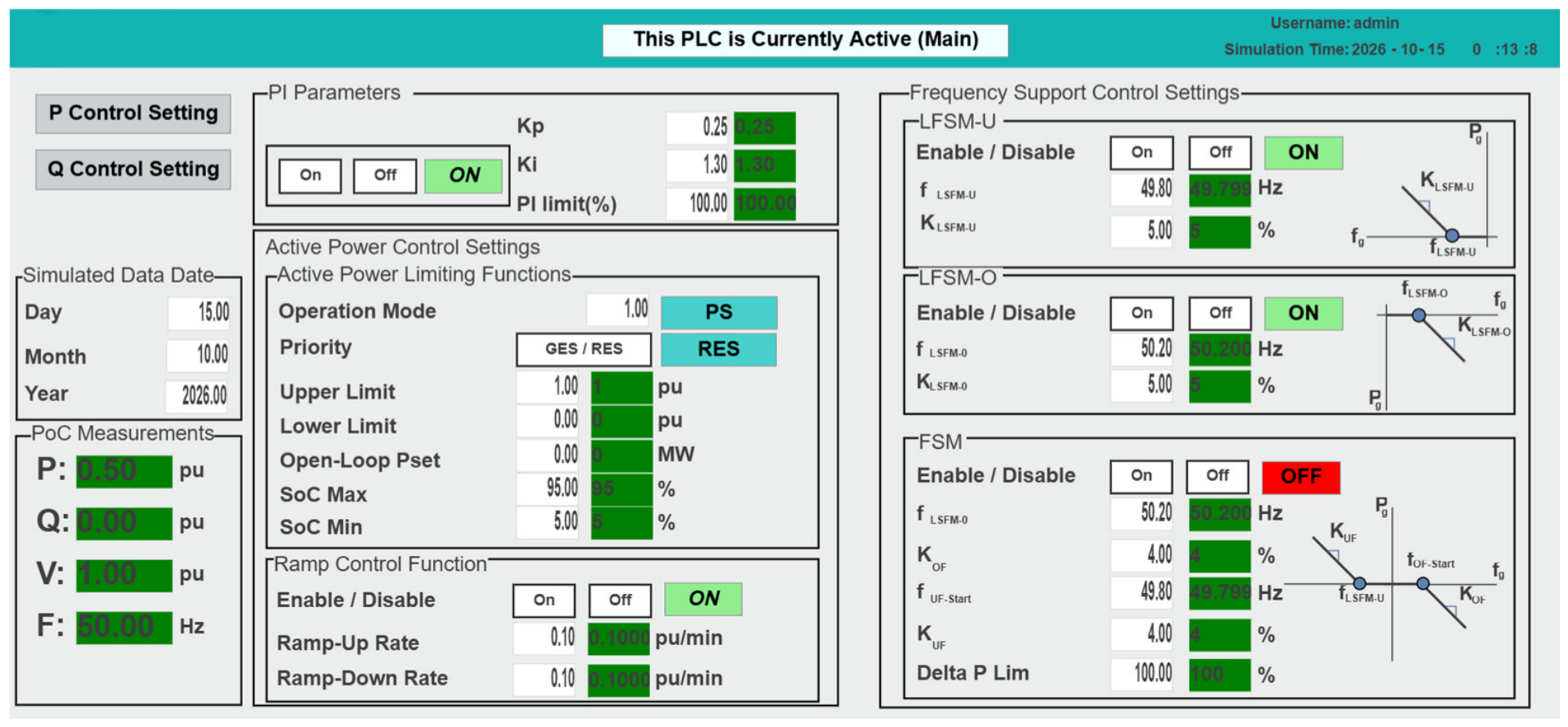
Figure A2 shows the reactive-power controller settings, including constant reactive power, power factor, and voltage control.
Figure A2.
PPC user interface for configuring reactive-power, power-factor, and voltage-control functions.
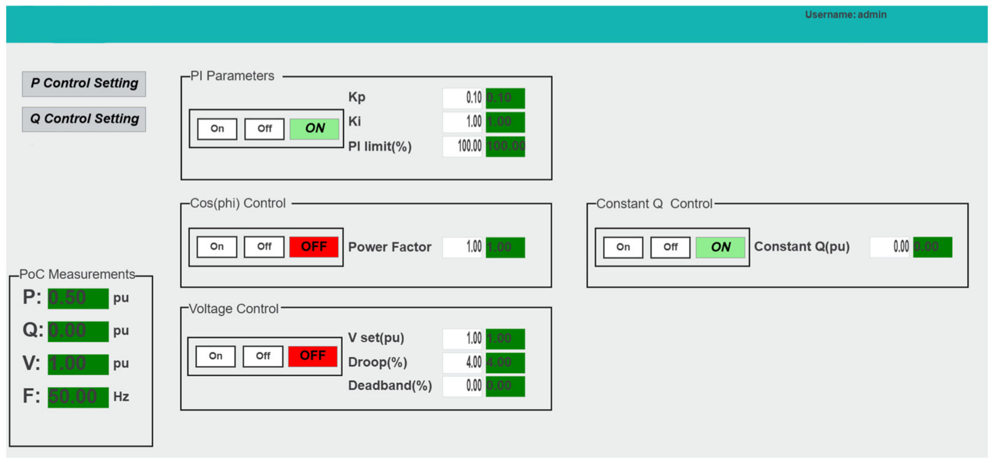
Figure A3 presents the MATLAB interface used to select the production dataset, start and stop the simulation, enable or disable Modbus communication, and monitor connection and simulation status.
Figure A3.
MATLAB user interface for dataset selection, simulation operation, and Modbus communication management.
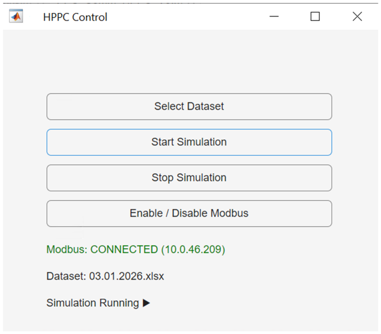
References
- Torres, J.R.; Ahmad, Z.; Veera Kumar, N.; Rakhshani, E.; Adabi, E.; Palensky, P.; van der Meijden, M. Power hardware-in-the-loop-based performance analysis of different converter controllers for fast active power regulation in low-inertia power systems. Energies 2021, 14, 3274. [Google Scholar] [CrossRef] [Scilit]
- Gupta, S.; Shukla, A.; Abusara, M. Integrated co-simulation and hardware-in-the-loop testing for microgrid. IEEE Trans. Ind. Electron. 2025, 72, 9082–9094. [Google Scholar] [CrossRef] [Scilit]
- European Commission. Commission Regulation (EU) 2016/631 of 14 April 2016 Establishing a Network Code on Requirements for Grid Connection of Generators (Text with EEA Relevance). Off. J. Eur. Union 2016, 112, 1–68. Available online: https://eur-lex.europa.eu/eli/reg/2016/631/oj/eng (accessed on 1 October 2026).
- Antoniadou-Plytaria, K.; Srivastava, A.; Ghazvini, M.A.F.; Steen, D.; Tuan, L.A.; Carlson, O. Chalmers campus as a testbed for intelligent grids and local energy systems. In Proceedings of the 2019 International Conference on Smart Energy Systems and Technologies (SEST), Porto, Portugal, 9–11 September 2019; IEEE: Piscataway, NJ, USA, 2019. [Google Scholar] [CrossRef] [Scilit]
- Asadi, E.; Keshavarzi, D.; Koehler, A.; Tashakor, N.; Goetz, S. Partial-Power Flow Controller, Voltage Regulator, and Energy Router for Hybrid AC-DC Grids. arXiv 2025, arXiv:2511.06335. [Google Scholar] [CrossRef] [Scilit]
- Estebsari, A.; Vogel, S.; Melloni, R.; Stevic, M.; Bompard, E.F.; Monti, A. Frequency control of low inertia power grids with fuel cell systems in distribution networks. IEEE Access 2022, 10, 71530–71544. [Google Scholar] [CrossRef] [Scilit]
- Clausen, C.S.B.; Jørgensen, B.N.; Ma, Z.G. A scoping review of In-the-loop paradigms in the energy sector focusing on software-in-the-loop. Energy Inform. 2024, 7, 12. [Google Scholar] [CrossRef] [Scilit]
- Hoke, A.; Chakraborty, S.; Basso, T. A power hardware-in-the-loop framework for advanced grid-interactive inverter testing. In Proceedings of the 2015 IEEE Power & Energy Society Innovative Smart Grid Technologies Conference (ISGT), Washington, DC, USA, 18–20 February 2015; IEEE: Toulouse, France, 2015. [Google Scholar] [CrossRef] [Scilit]
- Singh, A.; Prabakar, K. Controller-hardware-in-the-loop testbed for fast-switching sic-based 50-kw pv inverter. In Proceedings of the IECON 2018-44th Annual Conference of the IEEE Industrial Electronics Society, Washington, DC, USA, 21–23 October 2018; IEEE: Toulouse, France, 2018. [Google Scholar] [CrossRef] [Scilit]
- Gabbar, H.A. (Ed.) Microgrids: Planning, Protection and Control; MDPI-Multidisciplinary Digital Publishing Institute: Basel, Switzerland, 2022. [Google Scholar] [CrossRef] [Scilit]
- Schmitz, P.; Gonschor, D.; Jung, M. X-in-the-Loop Test Environment for Standardized Development of Photovoltaic Inverters. In Proceedings of the IEEE EUROCON 2023-20th International Conference on Smart Technologies, Torino, Italy, 6–8 July 2023; IEEE: Toulouse, France, 2023. [Google Scholar] [CrossRef] [Scilit]
- Singh, A.K.; Seethalekshmi, K. Hardware in the loop testing of converter control in solar PV and BESS based islanded microgrid. Eng. Res. Express 2024, 6, 035336. [Google Scholar] [CrossRef] [Scilit]
- De Carne, G.; Buticchi, G.; Liserre, M. Reverse power flow control in a ST-fed distribution grid. IEEE Trans. Smart Grid 2017, 9, 3811–3819. [Google Scholar] [CrossRef] [Scilit]
- Ahmad, Z.; Torres, J.R.; Veera Kumar, N.; Rakhshani, E.; Palensky, P.; van der Meijden, M. A power hardware-in-the-loop based method for FAPR compliance testing of the wind turbine converters control. Energies 2020, 13, 5203. [Google Scholar] [CrossRef] [Scilit]
- Gregorius Petra, T.N.A.; Irnawan, R. Design, Implementation, and Hil Testing of Internet-of-Things-Based Control System for PV-Battery Microgrid. In Proceedings of the 2025 International Seminar on Intelligent Technology and Its Applications (ISITIA), Surabaya, Indonesia, 23–25 July 2025; IEEE: Toulouse, France, 2025. [Google Scholar] [CrossRef] [Scilit]
- IEEE Std 1547-2018; IEEE Standard for Interconnection and Interoperability of Distributed Energy Resources with Associated Electric Power Systems Interfaces. IEEE: Piscataway, NJ, USA, 2018.
- Kikusato, H.; Orihara, D.; Hashimoto, J.; Takamatsu, T.; Oozeki, T.; Matsuura, T.; Miyazaki, S.; Hamada, H.; Miyazaki, T. Performance evaluation of grid-following and grid-forming inverters on frequency stability in low-inertia power systems by power hardware-in-the-loop testing. Energy Rep. 2023, 9, 381–392. [Google Scholar] [CrossRef] [Scilit]
- Campos, I.G.S.A.; Aragão, M.B.; Guerra, L.C.; Lisboa, L.A.C.; Malisano, G.; Ribeiro, A.S.; Santos, A.Á.; Melo, T.R. An automation system simulator for integration of a hybrid power plant: A real-unit case study. In Proceedings of the 2023 Workshop on Communication Networks and Power Systems (WCNPS), Brasilia, Brazil, 30 November–1 December 2023; IEEE: Toulouse, France, 2023. [Google Scholar] [CrossRef] [Scilit]
- Samano-Ortega, V.; Mendez-Guzman, H.; Padilla-Medina, J.; Aguilera-Alvarez, J.; Martinez-Nolasco, C.; Martinez-Nolasco, J. Control hardware in the loop and IoT integration: A testbed for residential photovoltaic system evaluation. IEEE Access 2022, 10, 71814–71829. [Google Scholar] [CrossRef] [Scilit]
- Liu, D.; Carta, D.; Xhonneux, A.; Muller, D.; Benigni, A. An MQTT gateway for HIL testing of energy systems. In Proceedings of the IECON 2022–48th Annual Conference of the IEEE Industrial Electronics Society, Brussels, Belgium, 17–20 October 2022; IEEE: Toulouse, France, 2022. [Google Scholar] [CrossRef] [Scilit]
- Pratticò, D.; Laganà, F.; Versaci, M.; Franković, D.; Jakoplić, A.; Vlahinić, S.; La Foresta, F. Enhancing power quality and reducing costs in hybrid AC/DC microgrids via fuzzy EMS. Energies 2025, 18, 5985. [Google Scholar] [CrossRef] [Scilit]
- Saha, S.K.; Arzani, A.; Salcedo, R.; Mahajan, S.M. Modbus tcp/ip based bess plant controller operations for a peak shaving application. In Proceedings of the 2025 IEEE Texas Power and Energy Conference (TPEC), College Station, TX, USA, 10–11 February 2025; IEEE: Toulouse, France, 2025. [Google Scholar] [CrossRef] [Scilit]
- IEC 61850-8-1:2011+AMD1:2020; Communication Networks and Systems for Power Utility Automation—Part 8-1: Specific Communication Service Mapping (SCSM)—Mappings to MMS (ISO 9506-1 and ISO 9506-2) and to ISO/IEC 8802-3. International Electrotechnical Commission: Geneva, Switzerland, 2020.
- Aboumadi, A.; Güneş, Z.; Yalman, Y.; Tan, A.; Terciyanlı, A.; Terciyanlı, E.; Bayındır, K.Ç. Design and Development of Energy Management System for Hybrid Microgrid. In Proceedings of the 2023 14th International Conference on Electrical and Electronics Engineering (ELECO), Bursa, Turkiye, 30 November–2 December 2023; IEEE: Toulouse, France, 2023. [Google Scholar] [CrossRef] [Scilit]
- Ampleman, S.; Sharma, H.; Mukherjee, S.; Glavaski, S. Control affine hybrid power plant subsystem modeling for supervisory control design. In Proceedings of the 2026 American Control Conference (ACC), New Orleans, LA, USA, 26–29 May 2026; IEEE: Toulouse, France, 2026. [Google Scholar]
- Liu, D.; De Din, E.; Carta, D.; Benigni, A. Controller hardware-in-the-loop testing of a multitimescale control architecture for multienergy systems. IEEE J. Emerg. Sel. Top. Ind. Electron. 2025, 6, 499–510. [Google Scholar] [CrossRef] [Scilit]
- Jonathan LeSage. Systems-Level Microgrid Simulation from One-Line Diagram, MATLAB Central File Exchange. 2026. Available online: https://www.mathworks.com/matlabcentral/fileexchange/67060-systems-level-microgrid-simulation-from-one-line-diagram (accessed on 19 February 2026).
- Kermani, M.; Adelmanesh, B.; Shirdare, E.; Sima, C.A.; Carnì, D.L.; Martirano, L. Intelligent energy management based on SCADA system in a real Microgrid for smart building applications. Renew. Energy 2021, 171, 1115–1127. [Google Scholar] [CrossRef] [Scilit]
- Cleveland, F.M. IEC 61850-7-420 communications standard for distributed energy resources (DER). In Proceedings of the 2008 IEEE Power and Energy Society General Meeting-Conversion and Delivery of Electrical Energy in the 21st Century, Pittsburgh, PA, USA, 20–24 July 2008; IEEE: Toulouse, France, 2008. [Google Scholar] [CrossRef] [Scilit]
- Honeth, N.; Yiming, W.; Etherden, N.; Nordström, L. Application of the IEC 61850-7-420 data model on a hybrid renewable energy system. In Proceedings of the 2011 IEEE Trondheim PowerTech, Trondheim, Norway, 19–23 June 2011; IEEE: Toulouse, France, 2011. [Google Scholar] [CrossRef] [Scilit]
- Energy Market Regulatory Authority (EPDK). Elektrik Şebeke Yönetmeliği [Electricity Grid Regulation], Annex 18, Resmî Gazete, no. 29013 (Mükerrer), 28 May 2014, Incorporating Amendments Through 29 December 2025 (Resmî Gazete, no. 33122). Available online: https://www.epdk.gov.tr/Detay/Icerik/3-6730/elektrik--sebeke- (accessed on 1 October 2026).
- Feng, J.; Cui, W.; Cortés, J.; Shi, Y. Online event-triggered switching for frequency control in power grids with variable inertia. IEEE Trans. Power Syst. 2025, 40, 3347–3360. [Google Scholar] [CrossRef] [Scilit]
- Zhang, Y.; Melin, A.; Djouadi, S.; Olama, M. Performance guaranteed inertia emulation for diesel-wind system feed microgrid via model reference control. In Proceedings of the 2017 IEEE Power & Energy Society Innovative Smart Grid Technologies Conference (ISGT), Washington, DC, USA, 23–26 April 2017; IEEE: Toulouse, France, 2017. [Google Scholar] [CrossRef] [Scilit]
- Breesam, W.; Alamian, R.; Tashakor, N.; Youcefa, B.E.; Goetz, S.M. Frequency Control in Microgrids: An Adaptive Fuzzy-Neural-Network Virtual Synchronous Generator. arXiv 2025, arXiv:2506.18611. [Google Scholar] [CrossRef] [Scilit]
- Hu, Y.; Zhang, R.; Lei, X.; Chao, P.; Jin, Y.; Zheng, J. Adaptive Frequency Regulation Control Method for Hybrid Renewable Energy Power Plants Based on Disturbance Intensity and Frequency Regulation Capability. In Proceedings of the 2025 7th International Conference on Energy Systems and Electrical Power (ICESEP), Wuhan, China, 20–22 June 2025; IEEE: Toulouse, France, 2025. [Google Scholar] [CrossRef] [Scilit]
- Laganà, F.; Pratticò, D.; Bibbò, L.; Pullano, S.A.; Calcagno, S. Integrated Fault Diagnosis in Grid-Connected PV Systems: Synergizing Infrared Thermography and Advanced Signal Processing. Appl. Sci. 2026, 16, 6036. [Google Scholar] [CrossRef] [Scilit]
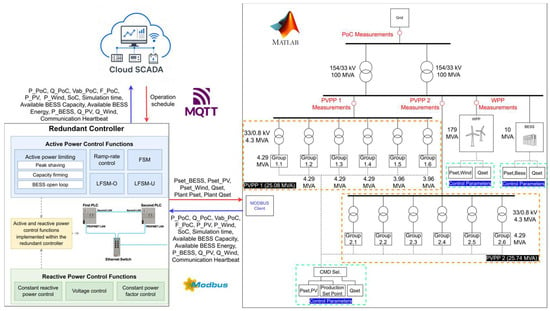
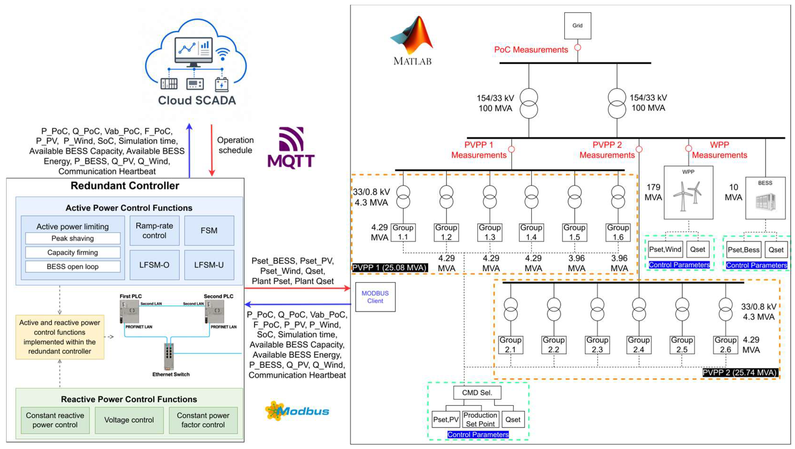
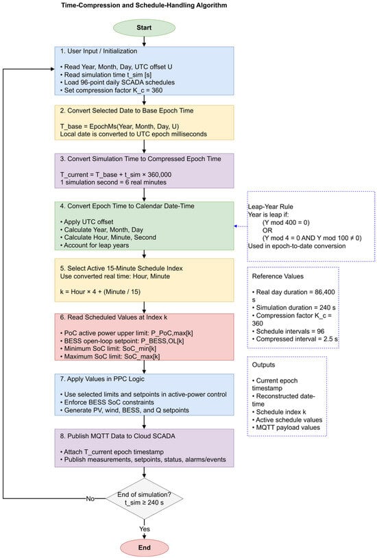
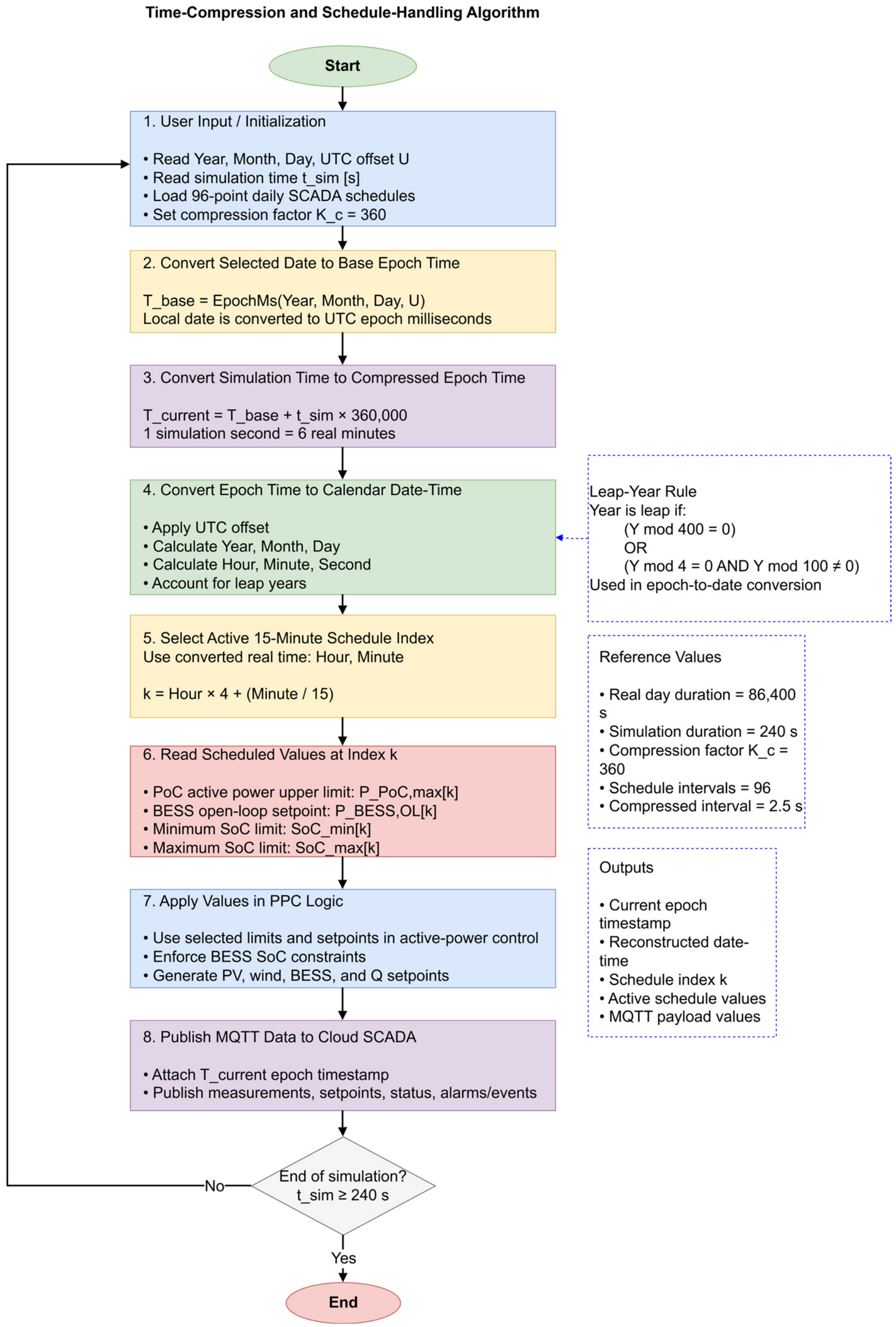
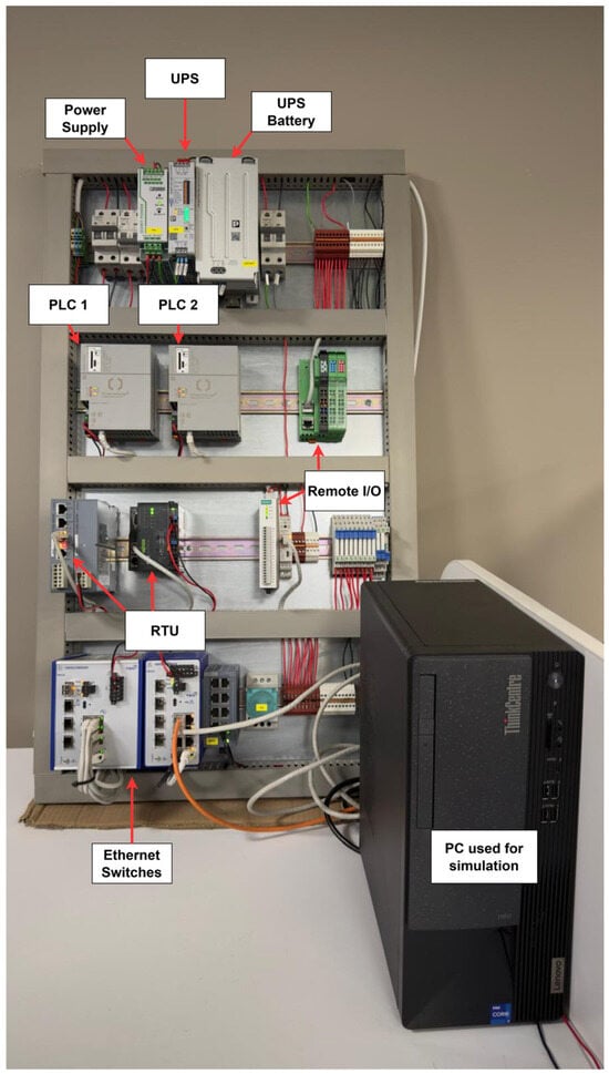
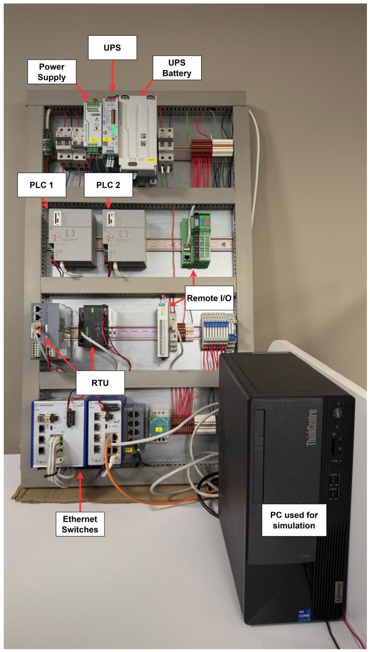
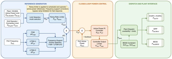
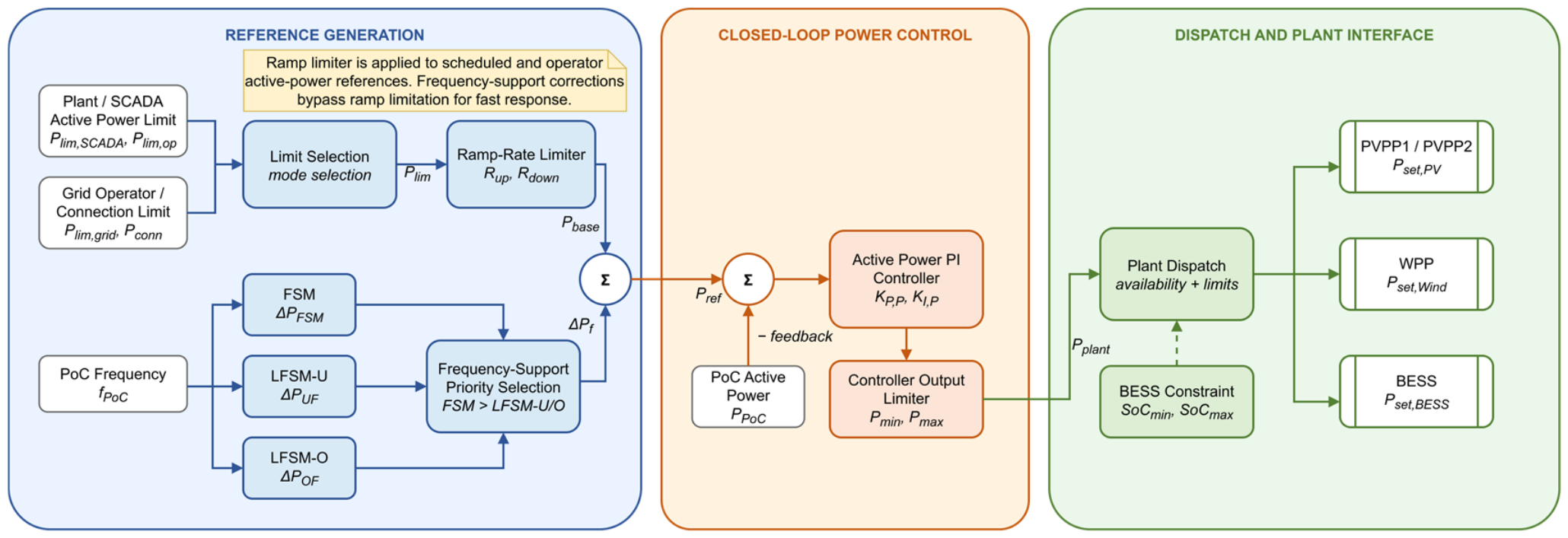
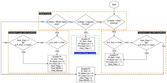
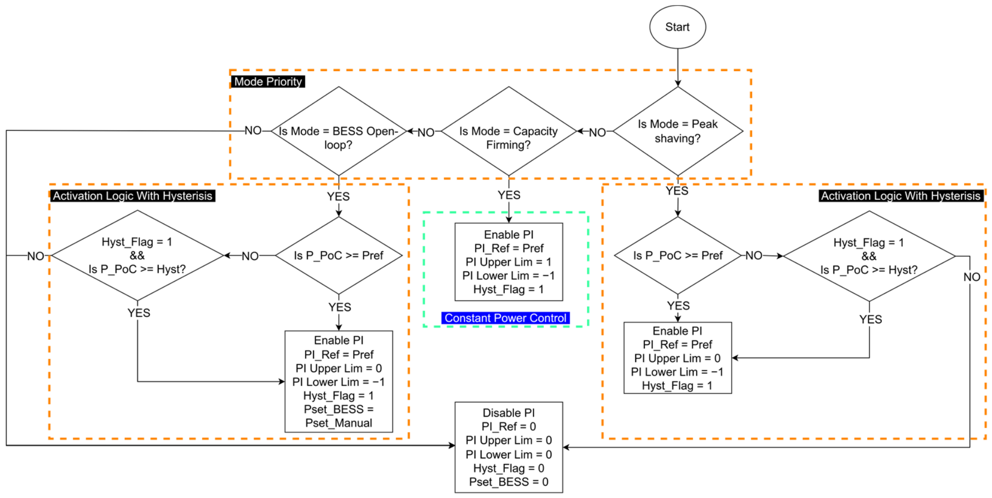
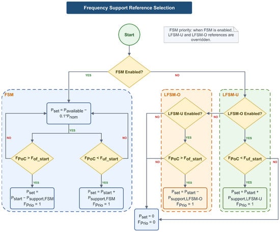
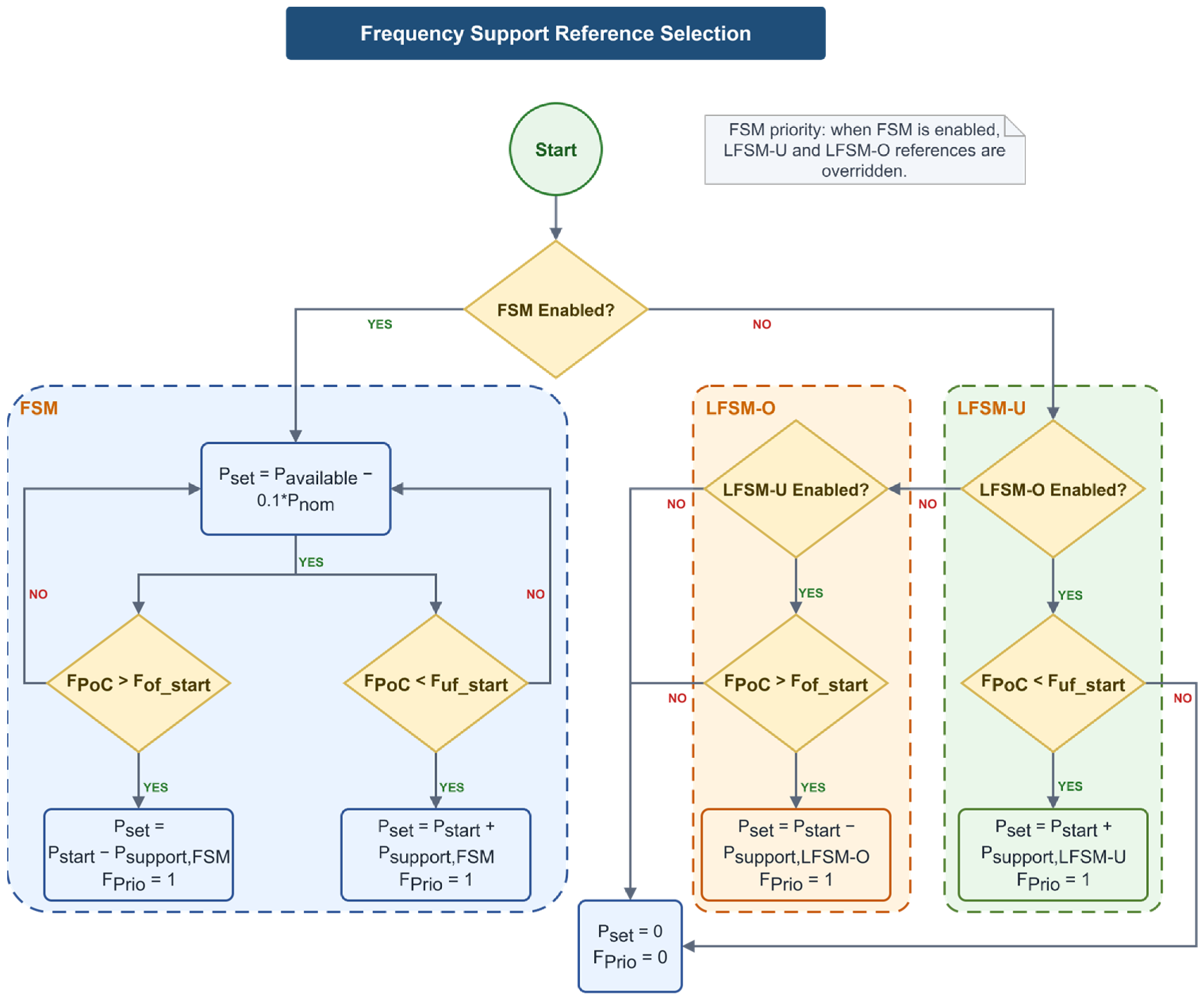
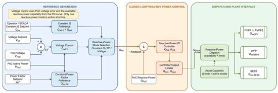
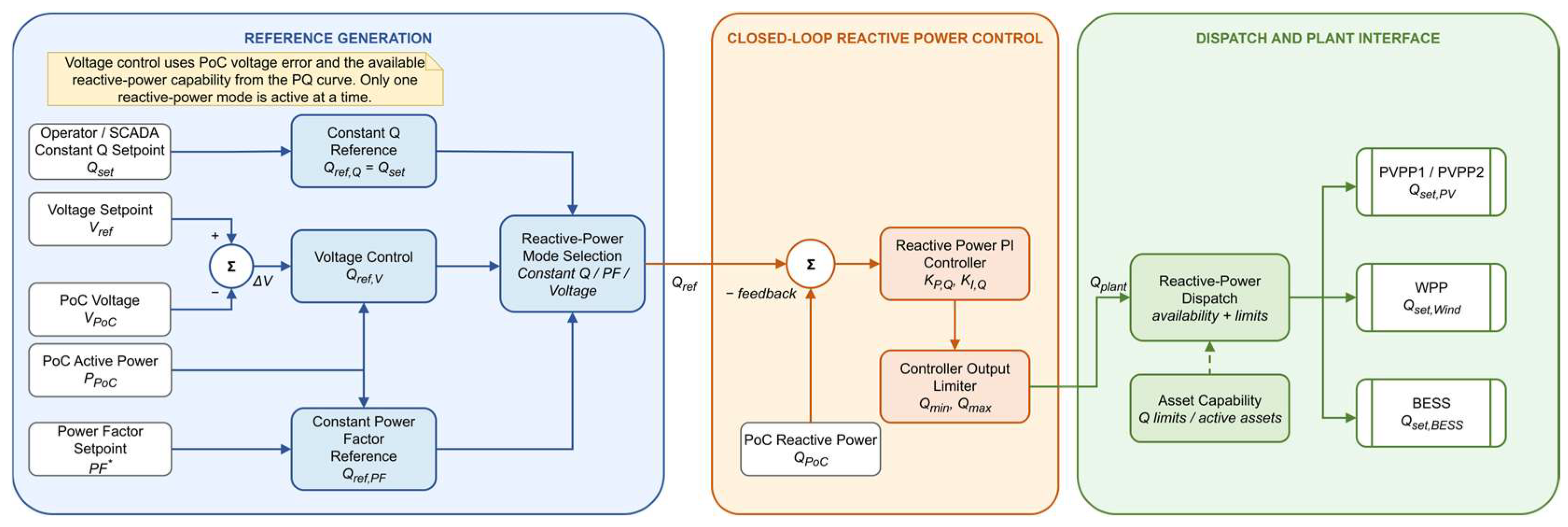
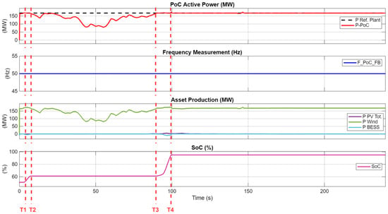
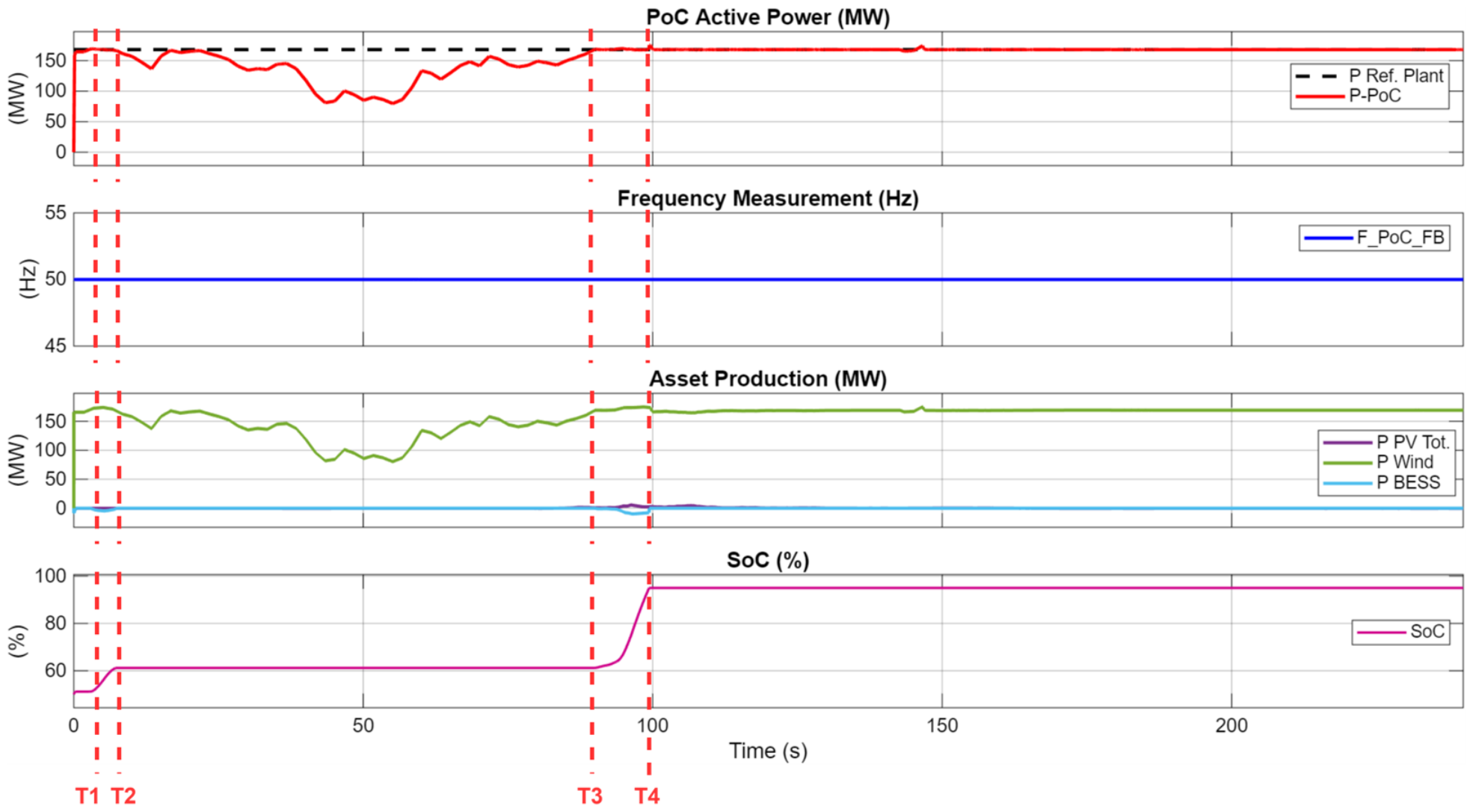
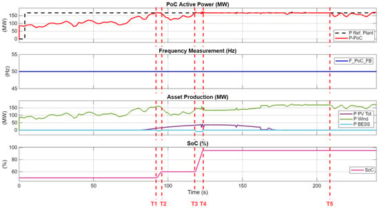
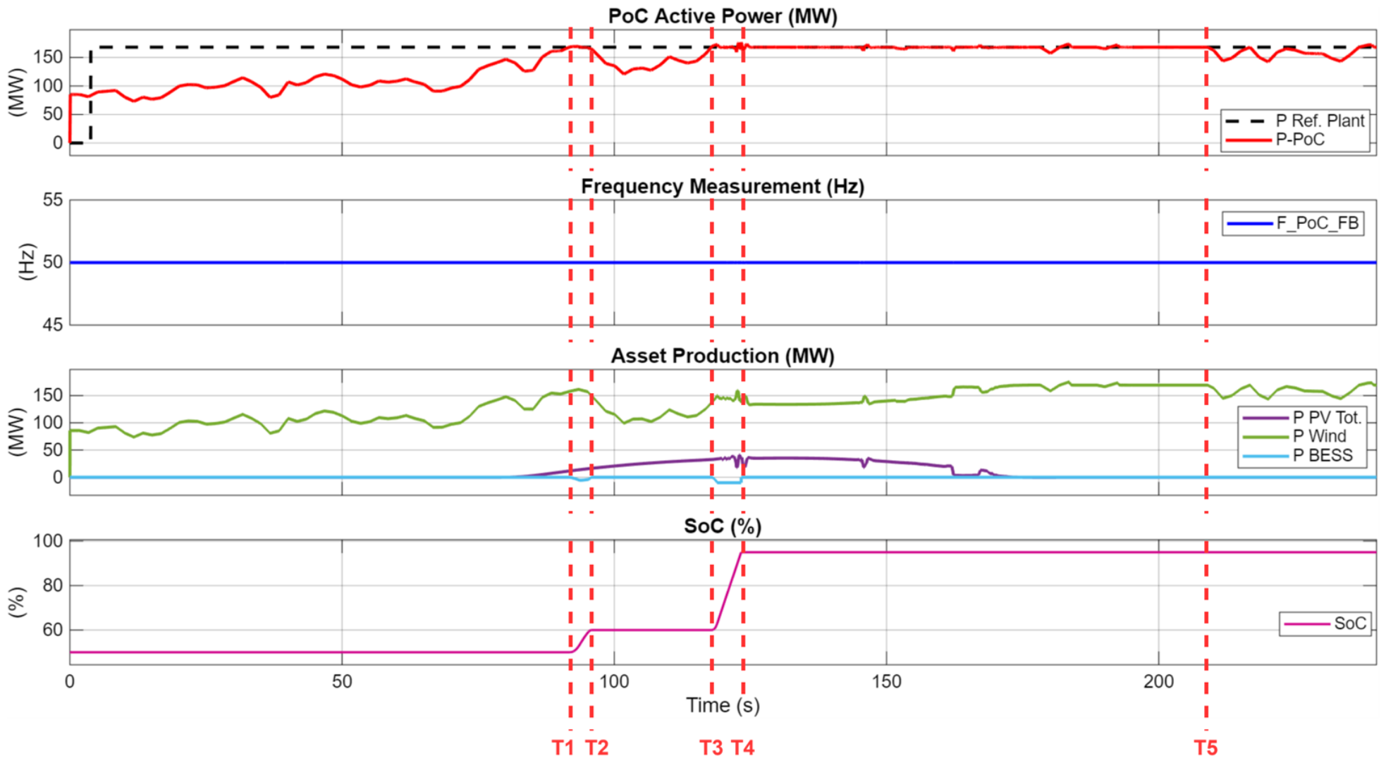
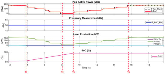
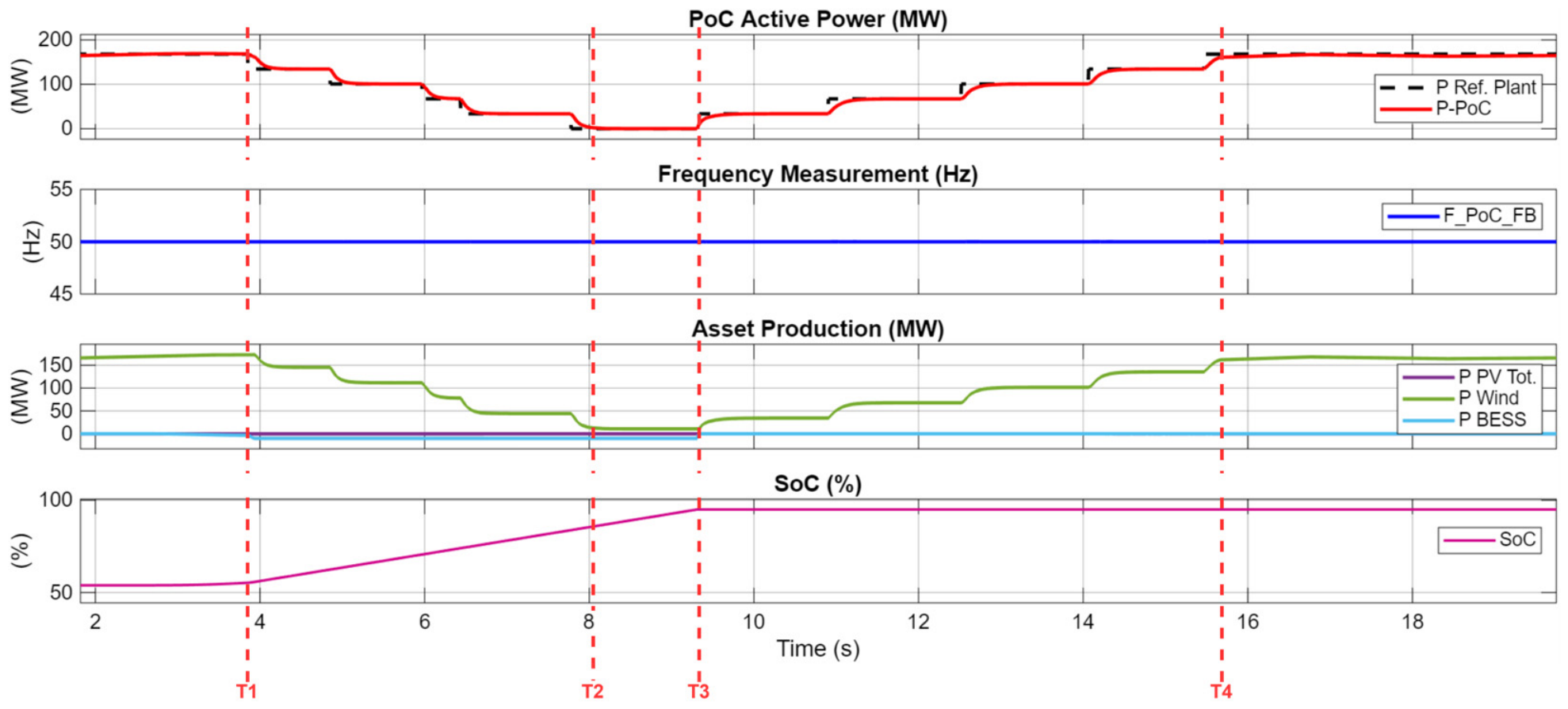
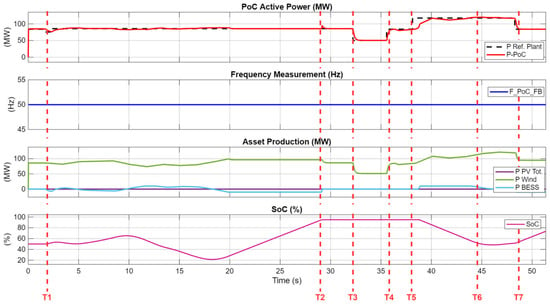
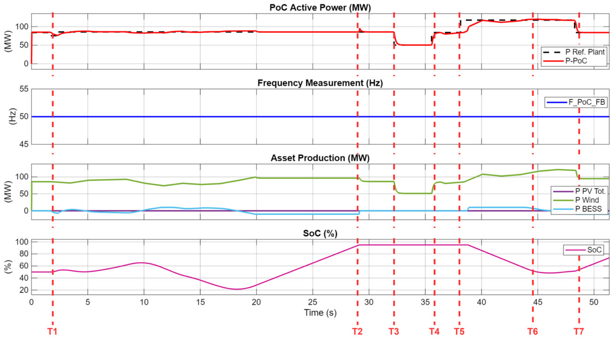
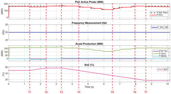
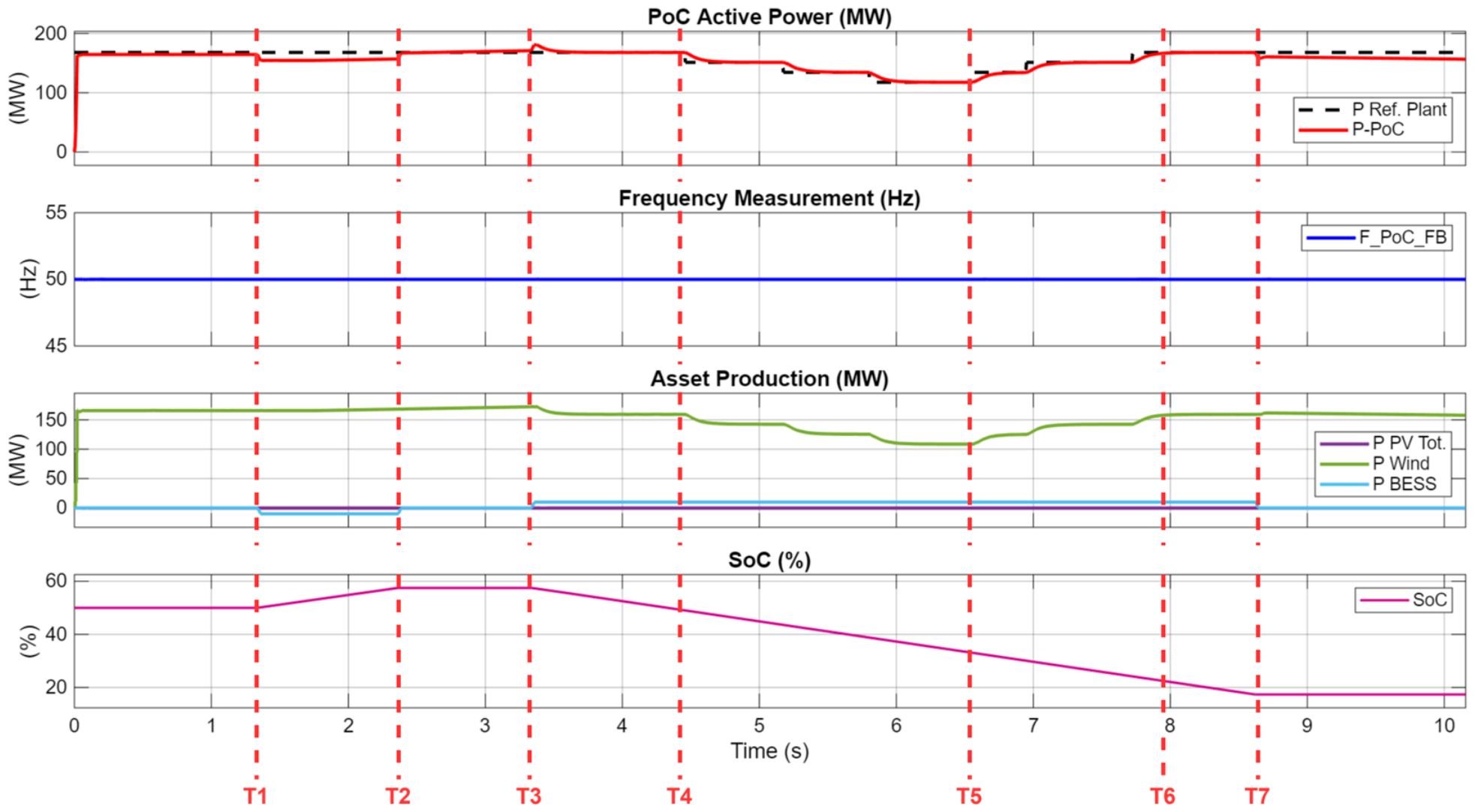
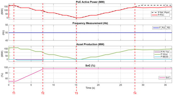
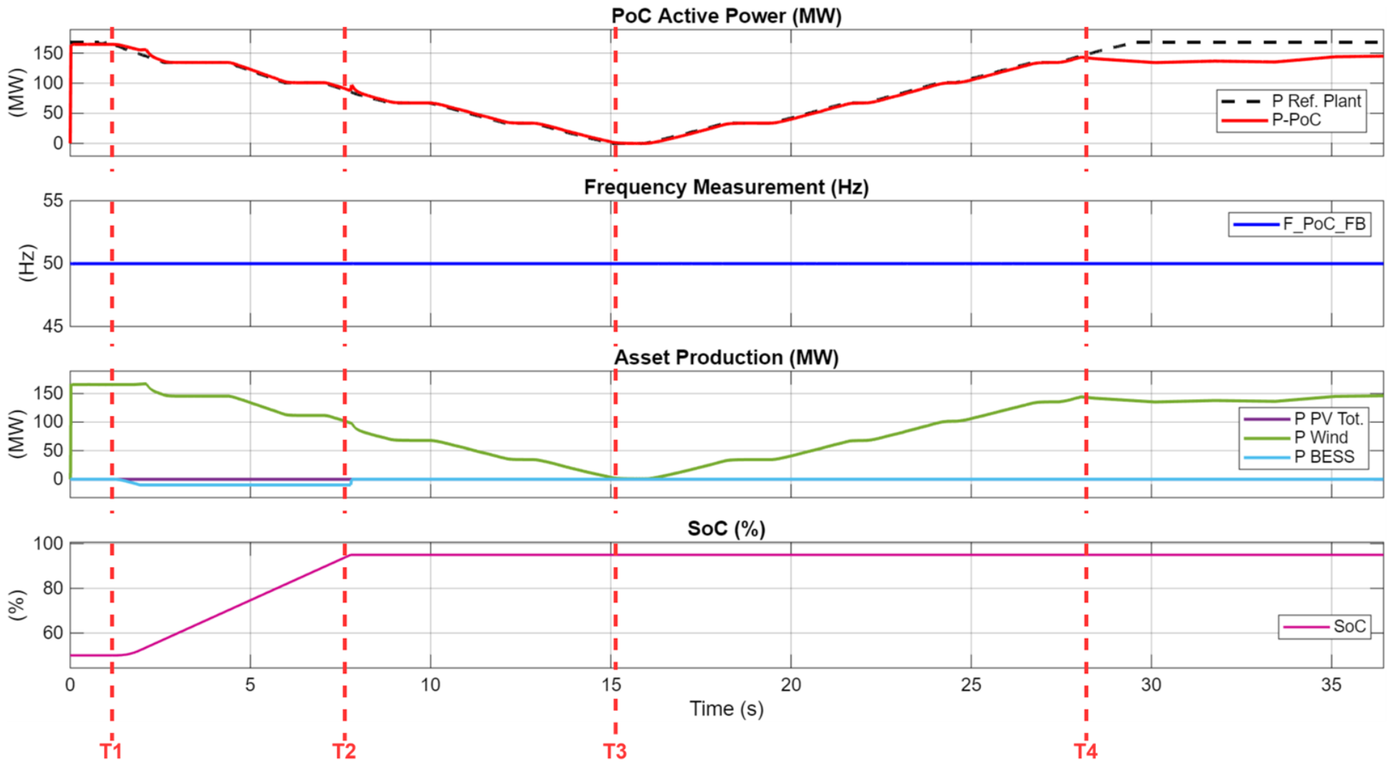
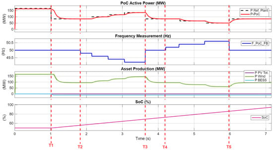
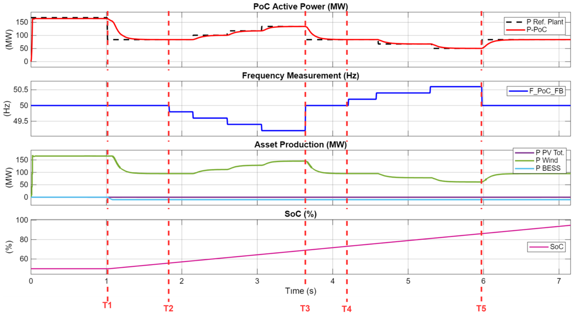
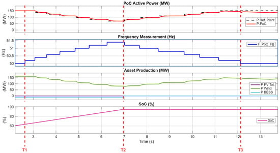
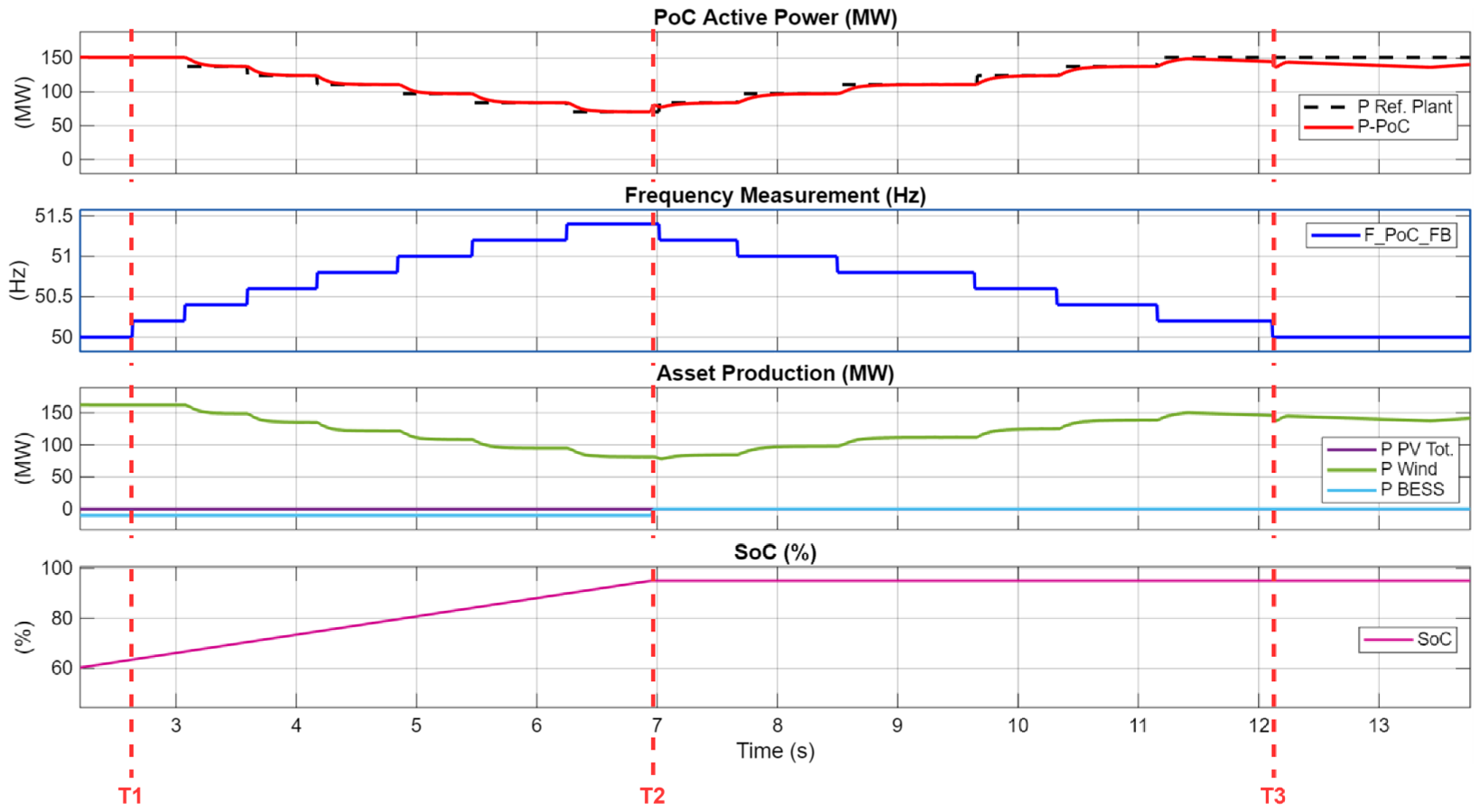
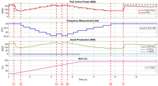
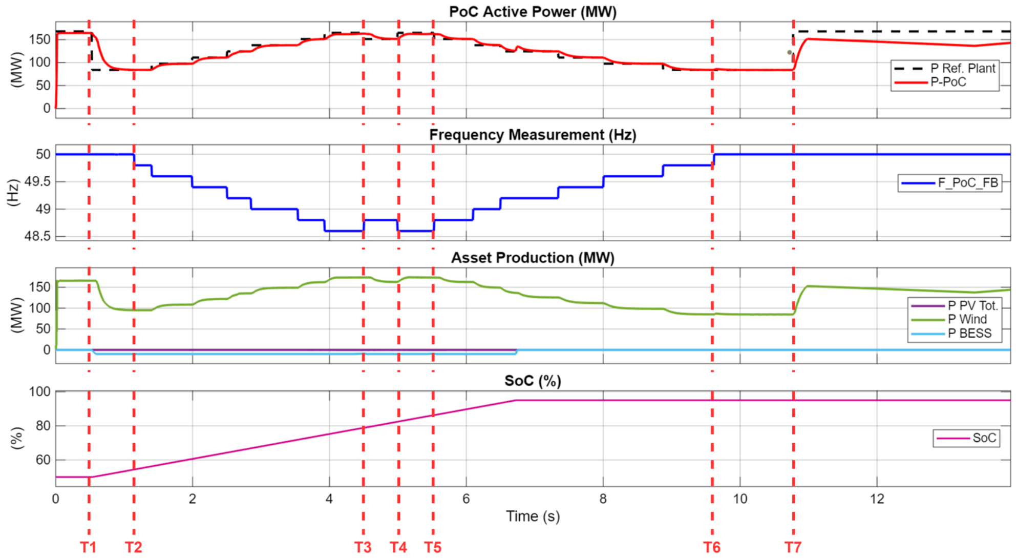
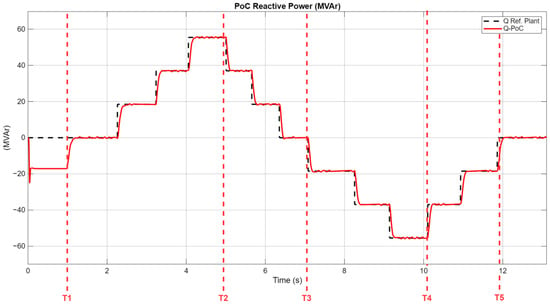
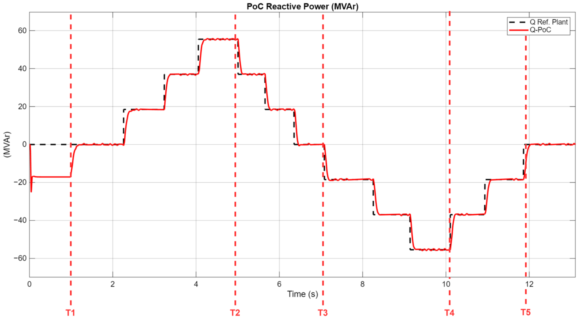
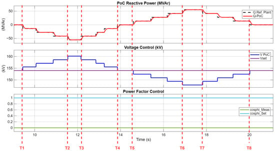
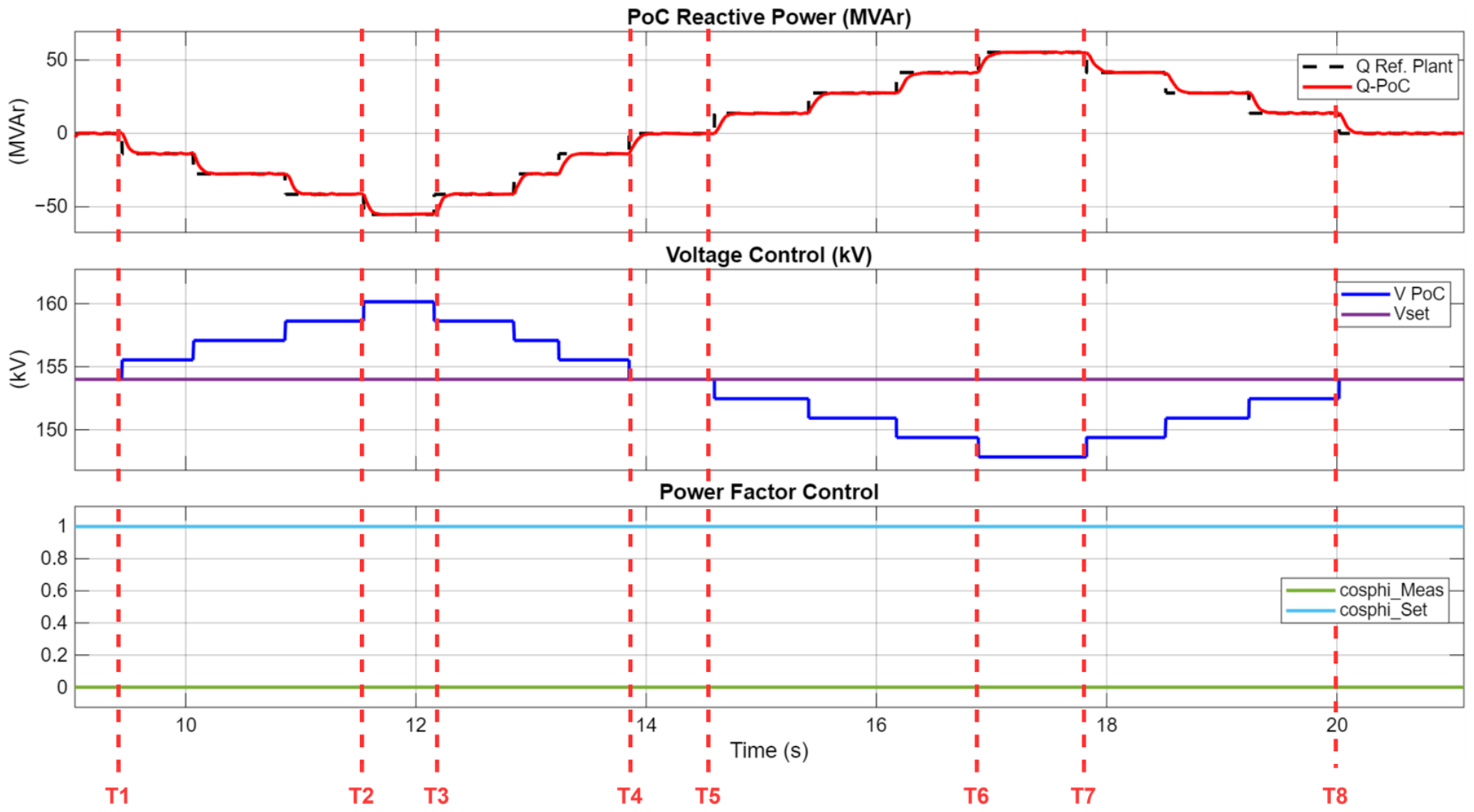
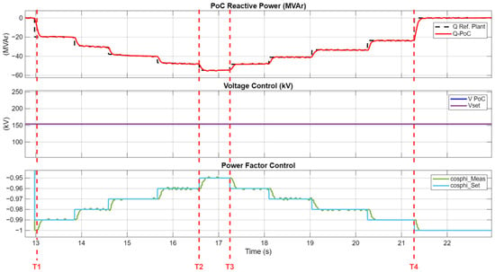
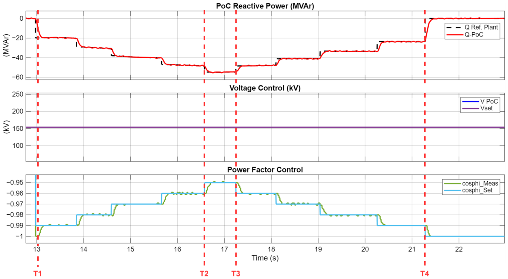
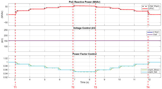
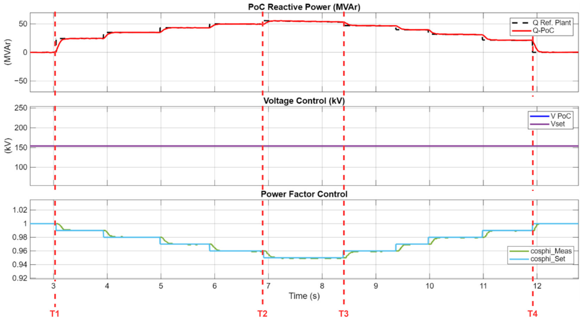
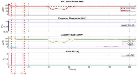
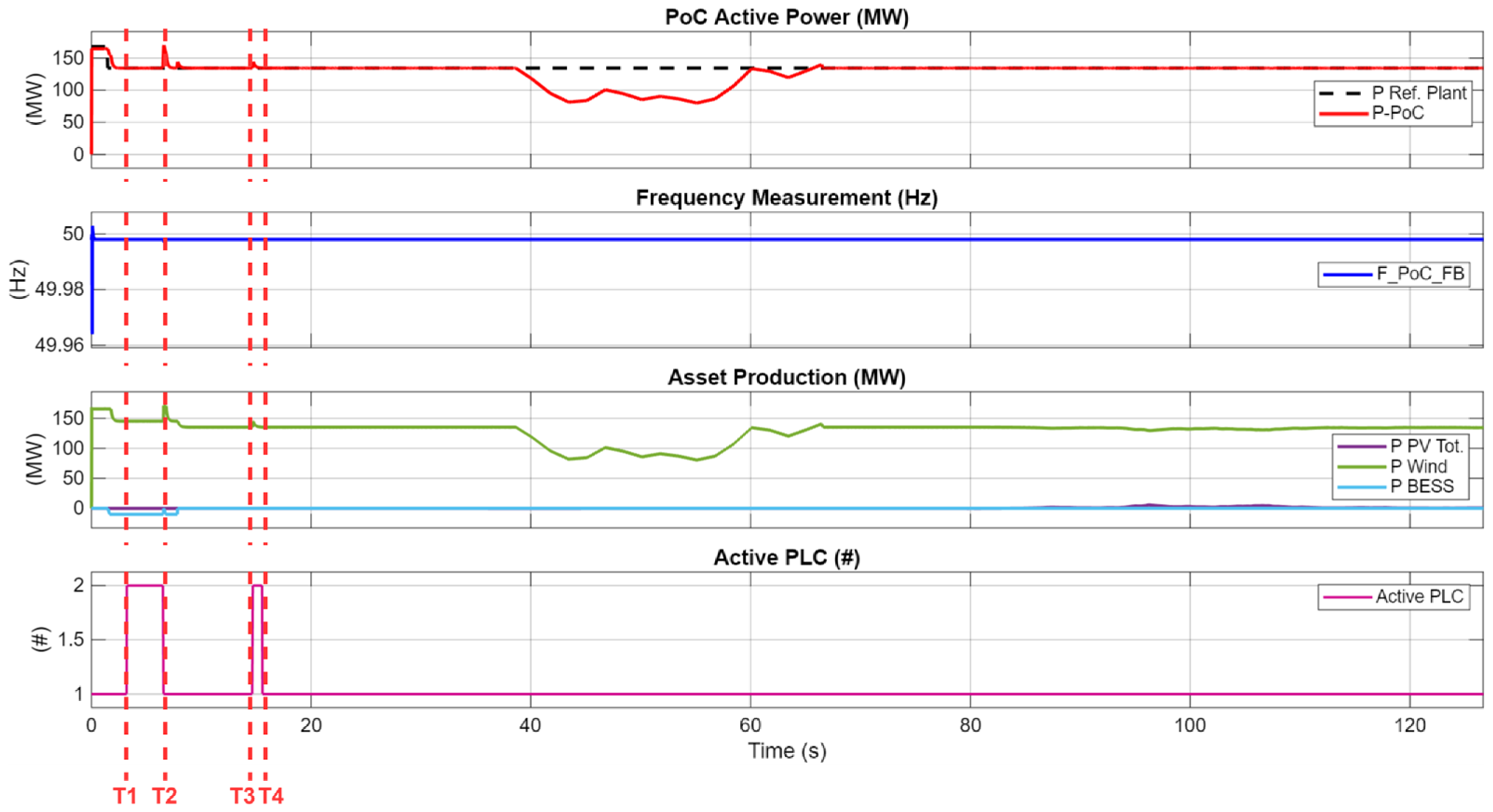
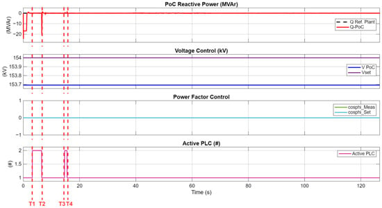
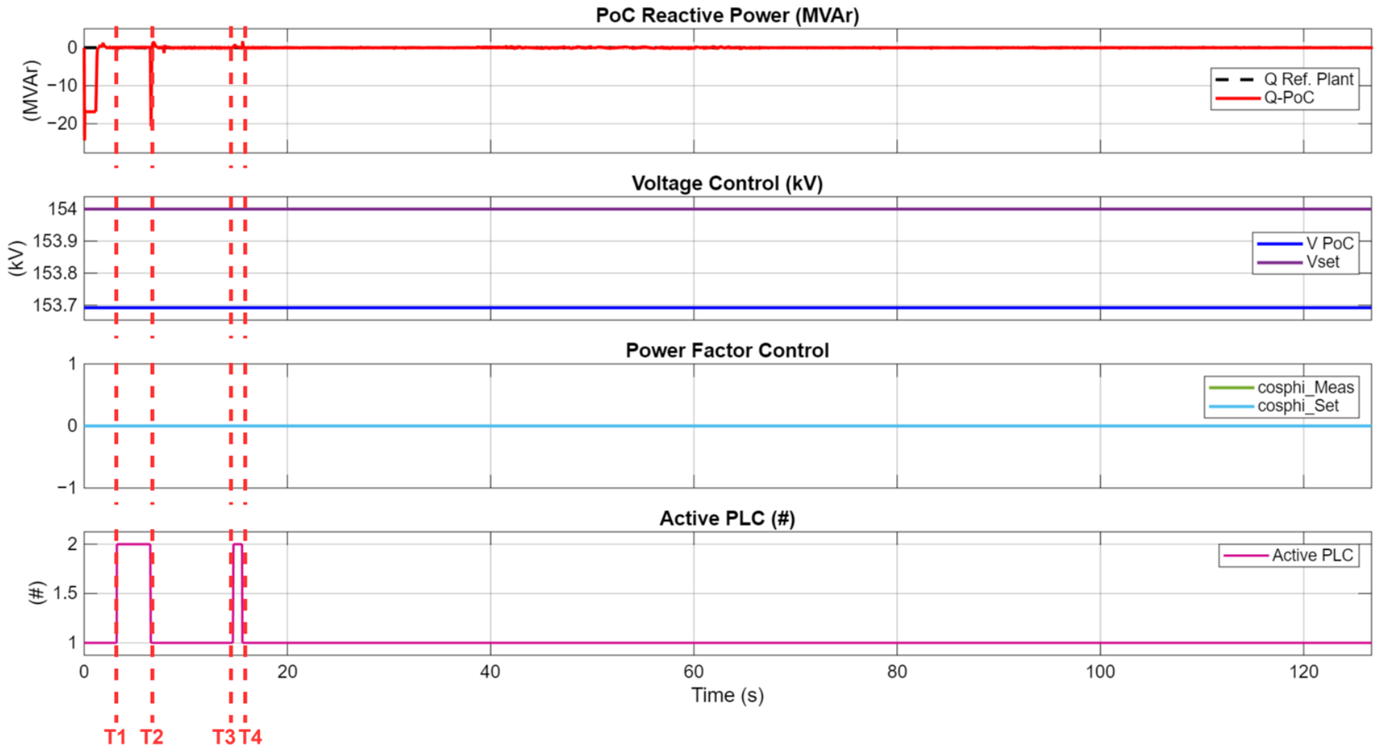

Disclaimer/Publisher’s Note: The statements, opinions and data contained in all publications are solely those of the individual author(s) and contributor(s) and not of MDPI and/or the editor(s). MDPI and/or the editor(s) disclaim responsibility for any injury to people or property resulting from any ideas, methods, instructions or products referred to in the content. |
© 2026 by the authors. Licensee MDPI, Basel, Switzerland. This article is an open access article distributed under the terms and conditions of the Creative Commons Attribution (CC BY) license.