


Abstract
To address the loss of high-quality solutions caused by decoupled topology and routing optimization, and the challenge of balancing robustness, delay, energy consumption and throughput in Ultraviolet C/Radio Frequency (UVC/RF) heterogeneous UAV swarm networks under extreme scenarios, this paper proposes a layered hybrid optimization framework termed Slime Mould Algorithm–Ant Colony Optimization–Grey Wolf Optimizer (SMA-ACO-GWO). It integrates the robust topology construction of the slime mould algorithm, the efficient multi-path routing of ant colony optimization, and the strong multi-objective search capability of the grey wolf optimizer. Joint optimization is achieved through four core mechanisms: slime mould topology-guided population initialization, ant colony routing-driven hierarchical leader mechanism, network state-aware dynamic weight adjustment, and topology-routing bidirectional feedback iteration. Simulation results show that compared with the standard GWO algorithm, the proposed algorithm reduces the number of convergence iterations by 60%, achieves the upper limit of 1.00 for the adopted robustness metric, reduces the average end-to-end delay by 86.2%, increases the normalized throughput by 77.9%, and reduces the total energy consumption by 18.0%. The algorithm features a low-complexity centralized architecture with distributed deployment potential. Its main optimization loop has a per-iteration complexity of O(n2), introducing low computational overhead and making it suitable for deployment on low-cost airborne platforms for highly dynamic and confrontational UAV swarm communication missions.
1. Introduction
The rapid growth of the low-altitude economy and the modernization of national emergency management systems are driving the evolution of UAV swarms from single-platform operations to coordinated multi-UAV missions [1]. In extreme scenarios where ground communication infrastructure is completely paralyzed by disasters such as earthquakes and floods, UAV ad hoc networks have emerged as the only viable means to maintain communication services, owing to their decentralized architecture and rapid deployment capability [2,3,4]. However, highly dynamic topologies cause on-demand routing protocols to frequently trigger network-wide route rediscovery, leading to a sharp surge in signaling overhead and a drastic decline in convergence speed. The limited battery capacity of small UAVs makes unreasonable relay selection highly prone to creating local “energy hotspots”, which further induces network partitioning or even full paralysis. In addition, a single radio frequency (RF) link can hardly strike a balance among transmission range, anti-interference performance and concealment in complex electromagnetic environments.
To overcome the limitations of single communication systems, the heterogeneous integration of ultraviolet C (UVC) and RF has emerged as a prominent research focus. UVC relies on non-line-of-sight (NLOS) scattering in the solar-blind band, featuring inherent anti-interference capability, low probability of interception and diffraction capability, making it suitable for short-range high-reliability relaying [5,6,7]. RF achieves wide-area coverage and high-speed transmission based on mature microwave technologies [8]. Existing studies on UAV-based ultraviolet communication have mainly focused on single-link topology control and routing optimization for homogeneous UVC networks: Zhao et al. proposed fault-tolerant topology control and formation topology optimization algorithms for cluster UAV ultraviolet covert communication networks [9,10], and Qiu et al. introduced an improved ant colony routing algorithm for ultraviolet communication networks [11]. However, these works only consider homogeneous UVC links and do not involve UVC/RF heterogeneous architecture or joint topology-routing optimization. The two types of links are highly complementary in terms of transmission mechanism and energy consumption characteristics, yet such heterogeneity also introduces new challenges to topology planning and routing optimization.
Existing studies fall into three broad categories. The first focuses on physical-layer channel design and power allocation. For example, Iqbal et al. investigated physical layer security enhancement for RIS-aided UAV heterogeneous links [12], and Xu et al. analyzed the secrecy performance of RF/UVC hybrid systems [13]. This line of research verifies the performance benefits of heterogeneous architectures but does not address network-layer collaborative optimization [12,13,14]. The second category adopts graph theory and mathematical programming methods, such as minimum spanning trees and connected dominating sets, for static topology planning [15,16,17]. These methods achieve optimal solutions for fixed topologies but tend to fail in highly dynamic topology scenarios due to their high computational complexity. The third category introduces bio-inspired algorithms (e.g., slime mould algorithm, ant colony algorithm, artificial bee colony algorithm), which have become the dominant research approach by virtue of their distributed self-organization properties [18,19,20]. Recent works further extend bio-inspired methods to adaptive topology control and energy-balanced routing for UAV networks, but they still follow a decoupled “topology-first, routing-later” design paradigm. For ultraviolet communication networks specifically, cluster-based bio-inspired algorithms have also been applied to balance energy consumption in reconnaissance UAV swarms [21], but they still follow the separate “topology-first, routing-later” optimization paradigm.
Nevertheless, direct application of these algorithms to UVC/RF scenarios still has limitations. The slime mould algorithm constructs robust topologies but exhibits weak routing optimization capability; the ant colony algorithm performs well in multi-path search but suffers from slow topology generation and a tendency to fall into local optima; the grey wolf optimizer has strong multi-objective optimization performance but its random initialization leads to slow convergence and unstable results. More critically, existing studies generally adopt a separate “topology-first, routing-later” optimization paradigm, ignoring the tight coupling between topology and routing, and thus making it difficult to obtain high-quality near-optimal solutions.
To address the above research gap, this paper proposes the SMA-ACO-GWO layered hybrid framework. The core contributions of this work are summarized as follows:
- (1)
- Three-stage hybrid initialization strategy. SlimeNet topology generation and ACO routing planning are combined to provide high-quality starting points for the grey wolf optimizer, mitigating the slow convergence and unstable performance caused by pure random initialization;
- (2)
- Ant colony routing-driven hierarchical leader mechanism. The population is divided into three specialized subpopulations for parallel search across topology and routing subspaces. This design expands the effective search range and reduces the risk of premature convergence in high-dimensional joint optimization scenarios;
- (3)
- Topology-routing bidirectional feedback mechanism. This mechanism enables co-evolution of topological structure and routing paths, breaking the conventional sequential “topology-first, routing-later” paradigm. Instead of a simple cascaded combination of existing modules, the organic integration of these components produces synergistic performance gains that cannot be achieved by any single mechanism alone.
In addition, a network state-aware dynamic weight adjustment scheme is integrated to balance global exploration and local exploitation by dynamically adjusting objective weights according to real-time network status.
2. System Model
2.1. Three-Dimensional UAV Network Scenario Model
Consider a UAV swarm network deployed in a three-dimensional Euclidean space Ω = [0, 300] × [0, 300] × [30, 150] m3. Let the node set be denoted as N = {1, 2, …, n}, where n = 50 represents the total number of nodes in the network. Node 1 is specified as the data source node S, Node 50 as the data destination node D, and the remaining nodes serve as relay nodes. The initial coordinates of the source node are fixed at [0, 0, 50]T, and those of the destination node are fixed at [300, 300, 50]T. The initial coordinates of relay nodes follow a uniform random distribution within the spatial region Ω.
A random walk mobility model with boundary damping constraints is adopted to simulate the dynamic flight characteristics of UAVs. The three-dimensional velocity vectors of nodes follow independent normal distributions, with a standard deviation of 0.5 m/s in the horizontal direction and 0.1 m/s in the vertical direction, and the time step is set to Δt = 2.0 s. To avoid excessively frequent topology changes, node positions are updated every 20 iterations, and mobility is only activated after the 30th iteration. When a node moves beyond the spatial boundary, the velocity component in the corresponding direction is reversed and multiplied by the damping coefficient 0.8, with its coordinates constrained within the boundary range.
A differentiated energy initialization strategy is applied to nodes. As the core communication endpoints of the network, the source and destination nodes are configured with an initial energy of 1000 J, while the initial energy of relay nodes follows a uniform distribution over 500 J~800 J. The remaining energy of nodes dynamically decays as communication links remain active. When the energy drops to 0, the node is completely disabled and loses all communication capabilities. The three-dimensional UAV scenario is illustrated in Figure 1.
Figure 1.
Illustration of the three-dimensional UAV network scenario.
2.2. UVC/RF Heterogeneous Communication Link Model
The transmission mechanism of solar-blind non-line-of-sight (NLOS) ultraviolet scattering is illustrated in Figure 2. Stratospheric ozone strongly absorbs solar ultraviolet radiation in the 200–280 nm band, resulting in extremely low background noise near the ground and the formation of a natural low-interference transmission window. Ultraviolet signals transmitted by communication nodes undergo multiple scattering by aerosols and molecules in the atmosphere and can be captured by the receiver under NLOS conditions without strict alignment between the transmitter and receiver. Constrained by the attenuation characteristics of ultraviolet transmission and the ozone layer altitude, the effective communication distance is limited to 50–150 m, and stable link performance is only available at altitudes below 100 m. This constraint provides a physical-layer basis for the subsequent reachability judgment of heterogeneous links.
Figure 2.
Schematic diagram of the UVC solar-blind scattering communication system.
The composition of the UAV-mounted ultraviolet bidirectional communication system is shown in Figure 3. The airborne communication terminal on a single UAV contains two independent branches: a transmit branch and a receive branch. The transmit branch performs data encapsulation, channel coding and modulation driving, and converts electrical signals into solar-blind optical signals through an ultraviolet LED array to emit into the atmosphere. The receive branch captures scattered optical signals via a photomultiplier tube (PMT) and recovers the original data after amplification, demodulation and decoding. UAVs on both sides complete uplink and downlink transmission simultaneously through the same scattering channel, realizing full-duplex bidirectional communication. Its hardware energy consumption characteristics and link transmission characteristics jointly form the modeling basis of the heterogeneous network cost model.
Figure 3.
Block diagram of the airborne ultraviolet communication system.
Based on the physical properties of UVC scattering and RF electromagnetic wave propagation, a heterogeneous link reachability criterion and an energy-aware joint cost model are established. For any two nodes i and j, a UVC link is reachable if and only if the Euclidean distance between nodes falls within 50–150 m and the flight altitudes of both nodes are below the 100 m assumed operational altitude threshold for UVC links. An RF link is reachable if and only if the Euclidean distance between nodes falls within 20–300 m.
On this basis, a heterogeneous link joint cost model is constructed, which comprehensively incorporates link distance, altitude difference and node remaining energy. First, an exponential energy factor is introduced [22]:
This factor generates a significant cost increase when node energy is nearly exhausted, thus naturally suppressing low-energy nodes from being selected as relays at the routing level.
For UVC scattering characteristics, a cost function consisting of distance cost, altitude difference cost and energy penalty term is designed [23]:
The distance cost adopts a quadratic form to reflect the rapid attenuation of UVC transmission quality with distance. The altitude difference cost is weighted at 0.3 to capture the significant impact of vertical distance on scattering links, and the energy factor is weighted at 0.2 to reflect the higher energy consumption of the UVC communication module.
For RF air-to-ground propagation characteristics, a cost function including a 1.5th-power distance term, a sigmoid-form long-distance surcharge and an energy penalty term is designed [24]:
The energy factor is weighted at 0.1 to reflect the higher energy efficiency of the RF communication module. A unified global altitude difference penalty is added to both types of links to ensure the vertical stability of the network topology. When both UVC and RF reachable links exist between two nodes, the link with lower cost is automatically selected for transmission.
All weighting coefficients are calibrated against measured parameters of commercial UVC/RF modules and published experimental data. The 0.3 altitude difference weight for UVC links reflects the significant impact of vertical scattering angle on received optical power, consistent with measurement results in [23]. The 0.2 energy factor weight for UVC and 0.1 for RF correspond to the measured power consumption ratio of typical solar-blind UV LED modules to 2.4 GHz RF transceivers. The 1.5th-power distance exponent for RF links matches the classic path loss model for terrestrial microwave communications.
Based on the physical properties of the two link types, a heterogeneous link reachability judgment and cost selection mechanism is established, and the complete flow is shown in Figure 4. For any node pair, the reachability of UVC and RF links is judged in parallel: the UVC link requires both flight altitude below the 100 m assumed operational altitude threshold for UVC links and a node distance within 50–150 m; the RF link requires a node distance within 20–300 m. If only one link type is reachable, it is adopted directly. If both are reachable, the comprehensive cost is calculated according to the weights of energy consumption, delay and robustness, and the link with the lower cost is selected. If neither is reachable, the node pair is judged to have no direct connection.
Figure 4.
UVC/RF heterogeneous communication link selection and judgment flow.
It should be noted that this paper focuses on the network-layer joint optimization of topology and routing, so the physical-layer UVC link model is reasonably abstracted. The impacts of atmospheric turbulence, aerosol scattering, transceiver elevation/azimuth angles, and background noise on link quality are equivalent to the constraints of communication range and link cost in the model. This simplification does not affect the core conclusion of this paper because the performance advantage of the proposed algorithm comes from the topology-routing joint optimization mechanism and hybrid meta-heuristic framework, rather than specific physical-layer link parameters. The proposed algorithm framework is universal and can be directly compatible with more precise UVC physical channel models by replacing the link reachability judgment and cost calculation modules, which will be further verified in future work.
2.3. Energy Evolution Model
To accurately quantify the impact of communication routing decisions on network energy distribution and lifetime, a refined energy consumption model for heterogeneous links is established. Link energy consumption is positively correlated with communication distance. Within each simulation step, the unit-distance energy consumption coefficient is 0.5 J/m for UVC links and 0.3 J/m for RF links. For an active link between node i and node j, the energy consumption per simulation step is equally shared by the two end nodes, as calculated by:
where αk denotes the unit-distance energy consumption coefficient corresponding to the link type, taking a value of 0.5 for UVC links and 0.3 for RF links, and dij represents the Euclidean distance between nodes. This linear model reasonably reflects the energy consumption differences among different communication systems while maintaining computational simplicity, facilitating the embedding of energy cost evaluation into routing decisions and topology optimization.
Econsume(i,j) = αk ⋅ dij
This sharing mechanism conforms to the actual physical characteristics of UAV communications: both the transmitter and receiver consume energy to complete signal transmission and reception.
In the proposed algorithm, node energy is updated after each main iteration based on the total energy consumption of active links in the current optimal topology, with link energy consumption equally shared by the two end nodes. The energy state serves as an input parameter for the next fitness calculation, realizing closed-loop optimization with energy awareness. The update formula is given by:
where Ni(t) denotes the set of neighbor nodes of node i at time t, and Econsume(i,j) represents the per-unit-time energy consumption of link (i,j). When the remaining energy of a node drops to 0, the node is deemed completely disabled. All its associated communication links are automatically disconnected, and the node no longer participates in subsequent routing forwarding and topology construction.
2.4. Network Resilience Evaluation Model
Network resilience describes the ability of UAV swarms to maintain core communication services under dynamic perturbations, and network robustness is adopted as its core quantitative metric in this work. This paper constructs a complete quantitative evaluation system from three dimensions: connectivity, invulnerability and topological stability, to fully characterize the survivability of the network under dynamic perturbations.
Source–destination connectivity is defined as the probability that at least one valid transmission path exists between the source node S and the destination node D at any simulation instant. This metric reflects the basic communication capability of the network and serves as the prerequisite for all performance indicators. Its calculation formula is:
where Tconnect denotes the total simulation duration during which the source–destination pair remains connected, and Ttotal represents the total simulation duration.
The network connectivity robustness metric is designed to quantify the communication guarantee capability and invulnerability potential of the topology structure, and is composed of basic connectivity and topological redundancy through weighted summation. Basic connectivity determines whether a valid transmission path exists between the source and destination nodes, taking a value of 1 when connected and 0 otherwise, reflecting the essential characteristic of topology connectivity. Topological redundancy is measured by the normalized average node degree: the higher the average node degree, the more alternative paths are available for switching when a single link fails, and the stronger the invulnerability potential of the topology. The weights of the two components are set to 0.7 and 0.3, respectively, and the calculation formula is given by:
where I(⋅) is an indicator function, which takes the value 1 if the source–destination node pair (S, D) is connected and 0 otherwise. denotes the average node degree of the network, which is normalized and truncated with an upper node degree limit of 8. It should be noted that the redundancy contribution gradually saturates at an average degree of approximately 2.4 in typical connected scenarios; the 8-degree upper limit serves as a unified normalization boundary to ensure numerical consistency across different network scales, rather than representing the actual saturation point of redundancy gain. The upper weight limit of this term is fixed at 0.3 to avoid excessive energy consumption caused by over-pursuit of redundancy. This connectivity-robustness metric is designed as a lightweight surrogate indicator for network resilience, and its physical rationality is verified as follows. First, the connectivity term directly reflects whether the core end-to-end transmission function is maintained, which is the most fundamental definition of network resilience. Second, the normalized average node degree term quantifies topological redundancy, which determines the number of alternative paths available for switching when single links or nodes fail. Empirical verification shows that this metric has a Pearson correlation coefficient above 0.92 with results from Monte Carlo random node failure tests across typical 50-node scenarios.
This metric can be computed rapidly with O(n2) complexity without repeated failure sampling, and can effectively reflect the connectivity reliability and redundant invulnerability of the topology while ensuring optimization efficiency. It is suitable for the fast iterative update mechanism of swarm intelligence algorithms.
Topological stability is measured by the fluctuation of the average node degree of the network. The average node degree is defined as the average number of neighbors of all nodes in the network, and its calculation formula is:
where M is the total number of valid links in the network, and n is the total number of network nodes. The average node degree reflects the connection density and redundancy level of the network. In this paper, the average node degree is maintained within a reasonable range around 3 through the topology decision mechanism, so as to guarantee connectivity while avoiding excessive energy consumption.
In addition to connectivity and stability, end-to-end delay is a core metric for measuring the real-time transmission capability of the network. In the proposed algorithm, end-to-end delay consists of two parts: propagation delay and per-hop fixed processing delay. For any link l = (i, j), its delay is calculated as:
where dij is the Euclidean distance between node i and node j (unit: m), v = 3 × 10⁸ m/s is the propagation speed of electromagnetic waves, converts the propagation delay into milliseconds (ms), and Dproc = 0.05 ms is the per-hop fixed processing delay. The end-to-end delay from the source node S to the destination node D is the sum of delays of all links along the path:
where P denotes the valid transmission path from S to D. If S and D are disconnected, the delay takes Dend-to-end = 100 ms (the maximum value).
It should be noted that the delay model described above represents a baseline propagation-processing delay formulated under ideal medium access control (MAC) layer assumptions. For practical communication systems, additional delay components arise from queuing, retransmission, and route switching processes. Queuing delay occurs when packets wait in node buffers prior to transmission; under the light-to-moderate traffic loads typical of emergency communication scenarios, this component typically accounts for 10–20% of the total end-to-end delay. Retransmission delay is induced by link errors and packet loss; for UVC links, which feature low background noise and high interference immunity, the retransmission rate remains below 1% under normal operating conditions, resulting in a negligible contribution to average delay. Route switching delay refers to the time required to switch from the primary path to a backup path following a failure. With precomputed link-disjoint backup paths, this switching delay is on the order of 5–10ms, which is an order of magnitude smaller than the route rediscovery delay associated with conventional on-demand routing protocols. In this work, the delay model focuses on the inherent propagation and processing delays determined by network topology and routing configurations, which represent the dominant components of end-to-end delay under normal operating conditions. The inclusion of additional practical delay components would increase the absolute delay values but would not alter the relative performance comparisons across different algorithms.
Network throughput is adopted to quantify the transmission carrying capacity of the network topology. The raw per-node throughput (in Mbps) is first computed as the total bandwidth of all active links divided by the total number of network nodes. It is then normalized by the maximum achievable per-node throughput of 10 Mbps under full connectivity, yielding the final normalized metric:
where Lactive denotes the set of valid links with weights above the activation threshold θ, Bi is the bandwidth of link i (10 Mbps for UVC links and 100 Mbps for RF links), Nnodes is the total number of network nodes, and the truncation threshold of 10 Mbps serves as the normalization baseline. This normalized metric is bounded within the [0,1] interval, which is consistent with the simulation results and values reported in the tables and figures throughout the manuscript.
This normalized metric captures the theoretical maximum per-node transmission capacity under ideal medium access control (MAC) conditions, where each link operates at full bandwidth without intra-link collisions. Physically, it represents the upper bound of network throughput capacity imposed by the topology structure, rather than the actual end-to-end delivered traffic volume. It quantifies the structural carrying capacity of the topology, independent of specific traffic patterns, routing schedules, and flow distributions.
In practical deployment, link contention and bottleneck effects reduce the actual achievable throughput. Specifically, when multiple flows share a single bottleneck link, the per-flow throughput decreases proportionally. However, for the topology-layer optimization problem addressed in this work, this upper-bound capacity metric reliably captures the relative transmission performance of different topologies.
The metric is normalized against the maximum achievable total bandwidth under full node connectivity, so it ranges strictly from 0 to 1. It is a widely adopted metric in topology optimization studies, as it allows direct comparison of the structural advantages of different network architectures independent of specific MAC protocols and traffic patterns.
2.5. Joint Optimization Problem Formulation
The resilient topology design and routing optimization problem for UVC/RF heterogeneous UAV networks is formulated as a constrained multi-objective optimization problem, with its core components defined as follows. The core decision variable is the weighted adjacency matrix W ∈ ℝn×n, where each entry wij ∈ [0,1] represents the weight of the link between node i and node j; a value of zero indicates no active link, while a positive value indicates an active connection. The type of each active link (UVC or RF) is determined by the distance and altitude criteria outlined in Section 2.2, and the set of routing paths = {P0,P1,…,PK}, including one primary path P0 and K backup paths P1,…,PK, is derived from the weighted adjacency matrix. Four objectives are considered simultaneously in the optimization: maximization of network robustness R (defined in Section 2.4, reflecting network connectivity and invulnerability), minimization of average end-to-end delay D (defined in Section 2.4, reflecting real-time transmission performance), maximization of total remaining energy E (described by the energy evolution model in Section 2.3, reflecting network operational lifetime), and maximization of normalized throughput T (defined in Section 2.4, reflecting network transmission capacity). The overall optimization problem is expressed as:
maxW F(W) = [R(W), − D(W), E(W), T(W)]T
The problem is subject to five categories of constraints. First, the link reachability constraint requires that every active link wij > 0 satisfies either the UVC or RF reachability criteria specified in Section 2.2. Second, the node degree constraint limits the number of active links per node such that di ≤ dmax, where dmax = 8 for source and destination nodes and dmax = 6 for relay nodes. Third, the link weight constraint enforces 0.2 ≤ wij ≤ 1.0 and matrix symmetry wij = wji. Fourth, the connectivity constraint ensures that at least one valid path exists between the source and destination nodes, such that R(W) > 0. Fifth, the energy constraint requires non-negative remaining energy for each node: Ei ≥ 0. This problem falls into the class of NP-hard combinatorial optimization problems, characterized by high-dimensional decision variables and multiple nonlinear constraints, which are challenging for conventional mathematical programming methods to solve efficiently. This property offers a theoretical rationale for adopting the swarm intelligence based hybrid optimization approach in this work.
3. Design of the SMA-ACO-GWO Hybrid Multi-Objective Optimization Algorithm
To address the loss of high-quality solutions caused by decoupled topology and routing optimization in UVC/RF heterogeneous UAV networks, this chapter presents the SMA-ACO-GWO layered hybrid multi-objective optimization algorithm. It achieves multi-objective collaborative optimization of robustness, delay, energy consumption and throughput through four core mechanisms: slime mould topology-guided population initialization, ant colony routing-driven hierarchical leader search, network state-aware dynamic weight adjustment, and topology-routing bidirectional feedback iteration.
All core control parameters of the algorithm are calibrated through preliminary simulation experiments to achieve an optimal trade-off between convergence speed and optimization performance. The symbols, baseline values and physical meanings of key parameters are summarized in Table 1. The design principles and operation procedures of each mechanism will be elaborated in the following subsections.
Table 1.
Core parameters of the proposed algorithm.
3.1. Overall Algorithm Framework
The complete workflow of the SMA-ACO-GWO algorithm comprises three stages: pre-optimization initialization, main iterative optimization, and optimal solution output, as outlined in Algorithm 1.
| Algorithm 1. SMA-ACO-GWO-based resilient UVC/RF heterogeneous UAV network construction. |
| SMA-ACO-GWO |
| Input: 3D position sequence pi(t), velocity sequence vi(t) of nodes; Communication parameters: UVC communication range Ruv, RF communication range Rrf, ozone altitude threshold Hozone, link activation threshold θ; Algorithm parameters: maximum iteration count Tmax, total population size Npop, number of topology wolves Ntopo, number of routing wolves Nroute, bidirectional feedback period Tfeedback, pheromone intensity Q, number of backup paths K; Energy parameters: initial node energy Einit, unit-distance energy consumption of UVC links Econsume_uvc, unit-distance energy consumption of RF links Econsume_rf. |
| Output: optimal topology adjacency matrix A∗; optimal primary path from source to destination Pprimary, backup path set Pbackup; optimal network robustness R∗, average end-to-end delay D∗, average remaining energy , network throughput T∗. |
| 1: Initialization |
| 2: Input total node count n_nodes; generate 3D randomly distributed node coordinates 3: Fix positions of source/destination nodes; set communication parameter set 4: Unify constraints including link activation threshold and maximum node connection count |
| 5: Initialize convergence history matrix: fitness_history = 0max_iter×4 |
| 6: Pre-optimization: SlimeNet topology generation |
| 7: Run SlimeNet for 100 iterations to generate initial conductivity matrix |
| 8: Extract upper triangular elements and flatten: Cflat = triu(C, 1)T |
| 9: Compute solution space dimension: |
| 10: Constrain conductivity range: Cij ∈ [0.2, 1.0]; ensure matrix symmetry C = CT |
| 11: Pre-optimization: ACO routing generation |
| 12: Under the constraint of slime mould topology, run ACO routing for 30 iterations |
| 13: Output optimal primary path primary and K − 1 link-disjoint backup path set backup |
| 14: Output pheromone matrix τ; extract and flatten upper triangular elements: τflat |
| 15: Force primary path link weights ≥ 0.6 to guarantee basic end-to-end connectivity |
| 16: Population initialization |
| 17: Initialize population matrix: |
| 18: Generate topology subpopulation (individuals 1–2): pop(i,:) = Cflat + (0, 0.05) |
| 19: Generate routing subpopulation (individuals 3–7): pop(i,:) = tflat + (0, 0.05) |
| 20: Generate resource subpopulation (individuals 8–35): large-amplitude Gaussian noise on Cflat |
| 21: Perform infeasible solution repair: constrain node connection count within hardware limit; set weights of excess links to 0.1 |
| 22: Fitness and Pareto set initialization |
| 23: Calculate four-dimensional fitness: fi = [fR, fD, fE, fT] |
| 24: Initialize Pareto optimal solution set ParetoSet; store all non-dominated solutions |
| 25: Main iteration loop |
| 26: for i = 1 → Npop do |
| 27: Match the subpopulation according to the individual index, and obtain the position vectors of α, β, δ leader wolves of the corresponding subpopulation |
| 28: for iter = 1 → max_iter do |
| 29: Compute current network states: global robustness R, average node degree , shortest path hop count path_length |
| 30: Re-run ACO under current topology to update pheromone matrix |
| 31: Normalize pheromone to obtain τflat |
| 32: Update conductivity vector: |
| 33: end if |
| 34: Sort by weighted fitness in the topology, routing and resource subpopulations respectively, and select the α, β, δ leader wolves |
| 35: Update the convergence factor: |
| 36: for i = 1 → Npop do |
| 37: Match the subpopulation by individual index; obtain α, β, δ positions |
| 38: for j = 1 → dim do |
| 39: Generate random numbers: r1,r2~U(0,1) |
| 40: Calculate encircling step coefficients: A = 2 a r1 − a, C = 2 r2 |
| 41: Candidate positions guided by three leaders: X1 = αj − A ⋅ |C ⋅ αj − pop(i,j)| X2 = βj − A ⋅ |C ⋅ βj − pop(i,j)| X3 = δj − A ⋅ |C ⋅ δj − pop(i,j)| |
| 42: Conductivity-weighted position update: |
| 43: end for |
| 44: Apply boundary constraints: all link weights within [0.1, 1.0] |
| 45: Perform infeasible solution repair: enforce node connection count limit |
| 46: Force primary path link weights ≥ 0.6 to maintain connectivity |
| 47: end for |
| 48: Recalculate four-dimensional fitness of all individuals |
| 49: Update Pareto set: add new non-dominated solutions, remove dominated ones |
| 50: Select current weighted optimal individual; store performance in fitness_history |
| 51: if iter > 80 and robustness SD over 20 generations < 0.03 and energy SD < 0.2 then |
| 52: Truncate fitness_history and break out of main loop |
| 53: end if |
| 54: end for |
| 55: Output |
| 56: Select global compromise optimal solution best_solution from ParetoSet via weighted sum method |
| 57: Map one-dimensional solution to 2D adjacency matrix; determine UVC/RF link types |
| 58: Calculate final performance metrics: R∗, D∗, , T∗ |
| 59: return ParetoSet, best_solution, fitness_history, A∗, Pprimary, Pbackup |
The pre-optimization stage is designed to mitigate the key limitations of the standard grey wolf optimizer: poor initial solution quality and extensive ineffective early searches resulting from random initialization. First, the SlimeNet algorithm is run to generate an initial conductivity matrix through the positive feedback mechanism of protoplasmic flow, building a globally robust topology skeleton. On this basis, an improved ant colony algorithm is executed to generate an end-to-end primary path and multiple link-disjoint backup paths, along with the routing pheromone matrix. The upper triangular elements of both matrices are flattened into one-dimensional vectors, and three subpopulations are generated by adding Gaussian noise of different amplitudes. The topology and routing subpopulations focus on the local refinement of topology structure and routing paths, respectively, while the resource subpopulation is assigned larger noise to preserve population diversity and avoid premature convergence.
During initialization, constraints on the lower link weight bound and upper node degree bound are applied, and mandatory repair is performed on infeasible solutions. Infeasible solution repair follows two core rules. First, the number of active connections per node shall not exceed the hardware-imposed limit (6 for relay nodes, 8 for source and destination nodes). Weights of redundant excess links are set to 0.1, which falls below the activation threshold θ and are thus treated as inactive weak links. Second, weights of all active links (weight ≥ 0.2) are maintained within the [0.2, 1.0] range.
This activation threshold rule is consistently applied across all modules of the algorithm, including topology construction, connectivity evaluation, routing computation, and fitness calculation.
The main iteration stage integrates three collaborative mechanisms. First, network state-aware dynamic weight adjustment: robustness, average node degree and path hop count are computed from the current optimal individual, and four-dimensional weights are output via an adaptive weight function. This allows the algorithm to automatically shift optimization priorities according to network connectivity, redundancy level and transmission efficiency. Second, topology-routing bidirectional feedback: for every fixed number of iterations, ant colony routing is re-run on the current topology to obtain an updated pheromone distribution. After normalization, the conductivity matrix is revised by weighted calculation, strengthening links that carry high-quality routes and suppressing redundant links, thus achieving co-evolution of topology and routing. Third, hierarchical leader parallel search: each subpopulation independently selects its own α, β and δ leader wolves, and individuals only update positions following the leaders of their own subpopulation. The topology subpopulation prioritizes robustness and energy efficiency, the routing subpopulation prioritizes delay and throughput, and the resource subpopulation explores potential superior regions. Running in parallel, the three cover different directions of the solution space and effectively mitigate population homogenization caused by single-leader guidance.
In the position update phase, a conductivity weighting factor is introduced into the standard grey wolf encircling and hunting formula. High-quality links are given larger step sizes to retain advantages, while low-quality links use smaller step sizes for fine tuning, further accelerating convergence. The energy convergence threshold εE = 0.2 corresponds to the standard deviation of normalized remaining energy, meaning the fluctuation of this indicator over 20 consecutive generations does not exceed 20% of the total energy range. The Pareto non-dominated solution set is updated after each iteration, and the algorithm terminates early when core indicators stay below the threshold for consecutive generations to reduce computational cost.
In the output stage, the linear weighted sum method is used to select the global compromise optimal solution from the Pareto front. The solution is mapped back to a two-dimensional adjacency matrix, and the communication mode (UVC/RF) of each link is determined by node altitude, distance and link activation threshold. Finally, the optimized topology, primary and backup path schemes, and four core performance metrics are output.
3.2. Pre-Optimization Stage: Slime Mould Topology and Ant Colony Routing Generation
The core objective of the pre-optimization stage is to provide high-quality initial solutions for the grey wolf optimizer, so as to mitigate its drawbacks of slow convergence and unstable results induced by random initialization.
3.2.1. Topology Skeleton Generation via SlimeNet Slime Mould Algorithm
The SlimeNet algorithm achieves self-organizing optimization of distributed network topologies by mimicking the foraging behavior of Physarum polycephalum. First, the algorithm initializes the conductivity matrix C with random values within [0.3, 1.0], sets the source node pressure to 10 and the destination node pressure to −5, forming the initial driving force for protoplasmic flow. In the main iteration, the pressure of all relay nodes is updated by:
where Di denotes the data rate of node i (set to 10 for the source node, −5 for the destination node, and random within 0.3~1.0 for relay nodes). The protoplasmic flow rate of each tube is calculated based on Poiseuille’s law:
Fij(t) = Cij(t) ⋅ (Pi(t) − Pj(t))
Following the positive flow feedback mechanism, tubes with larger flow rates gradually increase their conductivity, while those with smaller flow rates gradually shrink:
Meanwhile, a conductivity evaporation mechanism is introduced to simulate the natural attenuation effect of tubes over time, avoiding excessive convergence that leads to topological rigidity:
where Q = 1.5 is the conductivity enhancement coefficient, and dij(t) is the Euclidean distance between nodes. γ is the conductivity evaporation coefficient with a baseline value of 0.05; a larger value yields a stronger topological attenuation effect and higher population diversity. To ensure stable convergence of the algorithm, the conductivity is constrained within [0.05, 1.0], and the conductivity matrix remains symmetric throughout the process.
The hierarchical topology structure generated by the slime mould algorithm through flow positive feedback evolution is illustrated in Figure 5. In the figure, green and red five-pointed stars mark the source node S and destination node D, respectively, and gray dots represent relay nodes randomly distributed in three-dimensional space. Links of different colors correspond to different conductivity levels: dark blue backbone links have the highest conductivity and undertake the core end-to-end transmission function, while secondary links with high, medium and low conductivity form redundant topology layers, endowing the topology with inherent link-level invulnerability. This topology skeleton balances connectivity efficiency and redundant robustness, providing a high-quality topological baseline solution for the subsequent initialization of the grey wolf population.
Figure 5.
Simplified topology diagram of the slime mould algorithm.
3.2.2. Multi-Path Routing Generation via Improved Ant Colony Algorithm
Built upon the topology skeleton generated by the slime mould algorithm, an enhanced ant colony algorithm is deployed to generate initial multi-path routes. A topology prediction mechanism is introduced into the algorithm, which predicts node positions every 5 iterations to update the heuristic function in advance:
where ω = 0.7 is the prediction weight, ηcurrent is the current heuristic function, and ηpredicted is the predicted heuristic function. The transition probability is calculated as follows:
where τij(t) denotes the pheromone concentration, α = 1 is the pheromone importance factor, β = 1 is the heuristic function importance factor, and allowedk is the set of optional next-hop nodes for ant k.
ηcombined = (1 − ω) ⋅ ηcurrent + ω ⋅ ηpredicted
The pheromone is updated through a combination of global and local updates:
where ρ = 0.2 is the pheromone evaporation coefficient, Δτij is the pheromone increment, Q = 100 is the pheromone intensity, and Hk is the total hop count of the path traversed by the k-th ant.
τij(t + 1) = (1 − ρ) ⋅ τij(t)+Δτij
A greedy strategy is adopted for backup path selection. First, all feasible paths generated by the ant colony algorithm are collected and sorted in ascending order of path length. Then each path is checked in turn for shared links with the primary path. Paths with no shared links are added to the backup set until K − 1 paths are selected. This strategy achieves link-level fault tolerance while ensuring the quality of backup paths.
Finally, one primary path and two link-disjoint backup paths are generated, enabling millisecond-scale fast switching upon primary path failure. The multi-path routing structure generated by the ant colony algorithm under the constraint of slime mould topology is illustrated in Figure 6. In the figure, green and red five-pointed stars correspond to the source node S and destination node D, respectively. The blue solid line is the end-to-end primary path, which undertakes data transmission under normal conditions. The two dashed lines are link-disjoint backup paths with no shared links with the primary path, and can seamlessly take over transmission when the primary path fails due to node failure or link interruption. This multi-path architecture ensures transmission efficiency while providing link-level fault tolerance. The generated routing pheromone matrix provides a high-quality path baseline for the initialization of the grey wolf routing subpopulation.
Figure 6.
Schematic diagram of ant colony multi-path routing.
3.3. Slime Mould Topology-Guided Population Initialization
Conventional grey wolf optimizers rely on random initialization, which yields a large proportion of disconnected or low-quality solutions in the initial population and severely degrades convergence speed and final solution quality. This paper proposes a slime mould topology-guided population initialization method, which takes the conductivity matrix generated by SlimeNet as the baseline for the grey wolf initial population:
where Cflat denotes the upper-triangular vectorized representation of the conductivity matrix, and (0, 0.05) is Gaussian noise with zero mean and a standard deviation of 0.05. The low-amplitude noise is introduced to preserve population diversity while retaining the topological advantages of the slime mould algorithm. The resource subpopulation (individuals 8–35) is superimposed with Gaussian noise of 0.2 standard deviation to substantially increase population diversity and suppress premature convergence.
To guarantee basic connectivity, the weights of primary path links are enforced to be no less than 0.6:
where idx represents the index positions corresponding to the links of the primary path.
Xi,idx = max(Xi,idx, 0.6), ∀i = 1,2,…,Npop
3.4. Ant Colony Routing-Guided Hierarchical Leader Mechanism
Conventional grey wolf optimizers use a single leader to guide the entire population during search, resulting in a narrow search scope and a high risk of converging to local optima. For the high-dimensional search space of 1225 dimensions in a 50-node network, this paper proposes an ant colony routing-guided hierarchical leader mechanism, which divides 35 grey wolves into three subpopulations with clear functions:
- (1)
- Topology wolves (individuals 1–2);
Initialized by superimposing small-amplitude Gaussian noise on the slime mould conductivity baseline solution, focusing on optimizing the network topology to improve network robustness and energy efficiency.
- (2)
- Routing wolves (individuals 3–7);
Initialized by superimposing small-amplitude Gaussian noise on the ant colony routing pheromone baseline solution, focusing on optimizing routing paths to reduce end-to-end delay and improve network throughput.
- (3)
- Resource wolves (individuals 8–35);
Initialized by superimposing large-amplitude Gaussian noise on the slime mould conductivity baseline solution, accounting for 80% of the total population. They are responsible for global solution space exploration, preserving population diversity and avoiding premature convergence.
Each subpopulation selects its own α, β and δ leader wolves, and individuals within a subpopulation only update their positions following the leaders of their own group. This hierarchical mechanism enables parallel search in both the topology space and routing space simultaneously, significantly expanding the search range in high-dimensional space while ensuring the validity of search directions.
A conductivity weighting factor is introduced into the grey wolf position update formula. Links with higher conductivity are assigned larger position update step sizes, so that high-quality links are preferentially retained:
where X1, X2 and X3 are the position update results following the α, β and δ leader wolves, respectively.
The visualization of the solution space for the hierarchical leader search mechanism is illustrated in Figure 7. The high-dimensional topology-routing joint solution space is reduced to a three-dimensional coordinate system via principal component analysis, to intuitively present the spatial distribution pattern of the population during the iteration process. In the figure, the star-marked α leader wolf corresponds to the best-performing solution of the current subpopulation, and the circle-marked β and δ leader wolves represent the second-best and third-best solutions respectively. The three jointly form the encircling and hunting region around the optimal solutions. Gray scatter points denote ordinary grey wolf individuals, and dashed lines indicate the guidance paths for position update.
Figure 7.
Schematic diagram of solution space search for the hierarchical leader mechanism.
Ordinary individuals gradually converge toward the leader wolf group along the guidance paths. Combined with the parallel search mechanism of the three subpopulations, this scheme maintains global population diversity while ensuring local optimization precision, and effectively suppresses premature convergence of the algorithm.
3.5. Network State-Driven Dynamic Weight Adjustment
Multi-objective optimization with fixed weights fails to adapt to dynamic changes in network states, leading to severe performance degradation in certain scenarios. This paper proposes a network state-driven dynamic weight adjustment mechanism, which dynamically adjusts the weights of the four objectives according to the current network robustness R, average node degree and primary path hop count H:
When R < 0.7 and , network connectivity is insufficient. Robustness is prioritized, and the weight is set to [0.6, 0.15, 0.15, 0.1].
When R > 0.9 and , network connectivity redundancy is excessively high. Energy consumption reduction is prioritized, and the weight is set to [0.15, 0.15, 0.6, 0.1].
When R < 0.8, network performance is deteriorating. Topology reinforcement is prioritized, and the weight is set to [0.5, 0.2, 0.2, 0.1].
When H > 5 and , end-to-end transmission efficiency is low. Delay reduction is prioritized, and the weight is set to [0.15, 0.6, 0.15, 0.1].
In other cases, the balanced weight [0.25, 0.25, 0.25, 0.25] is adopted.
To ensure algorithm stability, strict boundary constraints are imposed on all parameters. This mechanism enables the algorithm to automatically adjust its optimization priorities according to network states, maintaining excellent optimization performance in dynamic topology scenarios.
The threshold values and weight combinations are determined based on extensive preliminary calibration experiments and engineering experience. The 0.7 robustness threshold corresponds to the minimum acceptable connectivity level for emergency communication networks. The 4.0 node degree threshold matches the optimal balance point between redundancy and energy efficiency verified by pre-experiments. The 5-hop path length threshold is consistent with typical end-to-end hop counts in the 50-node 300 m × 300 m scenario. The four-level weight set is designed to maintain a balance between targeted adjustment and algorithm stability, avoiding drastic oscillations caused by frequent weight switching.
3.6. Topology-Routing Bidirectional Feedback Mechanism
Topology and routing are tightly coupled: the topology structure defines the feasible routing space, while routing traffic distribution in turn shapes the topological evolution. This paper proposes a topology-routing bidirectional feedback mechanism to realize collaborative optimization of the two:
Every 20 iterations, the ant colony algorithm is re-run on the current topology to generate the latest routing pheromone matrix. After normalizing the pheromone matrix to the [0, 1] range, the slime mould conductivity vector is updated by a symmetric bidirectional adjustment mechanism:
where τflat is the upper-triangular vectorized representation of the normalized pheromone matrix, ⊙ denotes the Hadamard (element-wise) product, and clip(⋅,a,b) denotes element-wise clamping to the [a,b] interval.
Links with normalized pheromone above 0.5 receive increased conductivity (multiplier > 1), while links below 0.5 are suppressed (multiplier < 1). The conductivity is always constrained within the [0.2, 1.0] range throughout the process.
The updated conductivity matrix is then used to guide the position update of grey wolves. This mechanism feeds high-quality routing information discovered by the ant colony back to the slime mould topology, reinforcing high-traffic critical links while suppressing underused redundant links, and achieving co-evolution of topology and routing.
4. Simulation Experiments and Result Analysis
4.1. Simulation Environment and Parameter Settings
This section conducts simulation experiments based on a three-dimensional UVC/RF heterogeneous UAV network scenario, with all comparison algorithms executed under consistent conditions. A fixed random seed is adopted, and each experimental group is independently repeated 10 times. The mean of the performance metrics is taken as the final result to ensure statistical significance.
For statistical analysis, all comparison algorithms share the identical set of 10 independent random seeds to ensure consistent initial conditions and fair comparison. The standard deviation (SD) and 95% confidence interval (CI) of each metric are calculated based on the 10 independent runs. The Wilcoxon signed-rank test is employed to verify the statistical significance of performance differences between the proposed algorithm and baseline algorithms, with the significance level set at p < 0.05.
The simulation area is defined as 300 × 300 × 120 m3 with an altitude range of 30–150 m, containing 50 UAV nodes. The source node and destination node are deployed at (0, 0, 50) m and (300, 300, 50) m, respectively, while relay nodes are initially distributed uniformly at random. Nodes follow a random walk mobility model with boundary damping constraints, with a horizontal velocity standard deviation of 0.5 m/s and a vertical velocity standard deviation of 0.1 m/s. Node positions are updated every 20 iterations. When a node moves beyond the boundary, its velocity in the corresponding direction is reversed and multiplied by a damping coefficient of 0.8.
UVC links have an effective communication range of 50–150 m and are only available at altitudes below 100 m. RF links cover a range of 20–300 m and operate normally at all altitudes. The unit-distance energy consumption coefficient is 0.5 J/m for UVC links and 0.3 J/m for RF links, and the total energy consumption of a link per step is equally shared by its two end nodes. The source and destination nodes are configured with an initial energy of 1000 J, while the initial energy of relay nodes follows a uniform distribution from 500 J to 800 J.
All core simulation parameters are tuned through multiple preliminary tests to strike a balance between convergence speed and optimization performance. Population size, maximum iteration count and communication parameters are kept identical for all comparison algorithms to guarantee fair comparison. The full set of simulation parameters is summarized in Table 2.
Table 2.
Simulation parameters.
4.2. Comparative Experiments Under the Benchmark Scenario
Under the benchmark scenario of a 50-node 3D UVC/RF heterogeneous network, three algorithms are selected as comparison baselines: the standard Grey Wolf Optimizer (GWO), the Ant Colony Routing-guided Grey Wolf Optimizer (ACO-GWO), and the Slime Mould Algorithm (SMA)-guided Topology Grey Wolf Optimizer (SMA-GWO). GWO adopts random initialization and a single leader guidance mechanism. ACO-GWO initializes its population with ant colony routing results. SMA-GWO completes population initialization under the guidance of slime mould topology.
In addition to the three GWO-family baselines, two classical multi-objective optimization algorithms, the Non-dominated Sorting Genetic Algorithm II (NSGA-II) and the Multi-Objective Evolutionary Algorithm based on Decomposition (MOEA/D), are implemented for quantitative comparison. Both algorithms are configured with the same population size of 35, maximum iteration count of 200, network scenario and parameter settings as the GWO-family algorithms to ensure fair comparison. Their convergence curves are shown in Figure 8 and Figure 9 and their steady-state performance metrics are summarized in Table 3 for intuitive comparison.
Figure 8.
Network robustness convergence curves of different algorithms.
Figure 9.
Average end-to-end delay convergence curves of different algorithms.
Table 3.
Steady-state performance comparison of different algorithms under the benchmark scenario.
Quantitative comparison results show that NSGA-II converges slowly in this 1225-dimensional high-dimensional joint optimization problem due to its random initialization and general-purpose crossover operator. After 200 iterations, its final robustness is 0.712 ± 0.031, average end-to-end delay is 0.584 ± 0.042 ms, and normalized throughput is 0.726 ± 0.035. MOEA/D achieves better performance than NSGA-II with its decomposition-based search mechanism, with a final robustness of 0.795 ± 0.027, delay of 0.462 ± 0.037 ms, and throughput of 0.803 ± 0.031.
Both classical multi-objective algorithms significantly underperform the proposed SMA-ACO-GWO algorithm. This performance advantage stems from the integration of domain-specific prior knowledge of network topology and routing into the hybrid optimization framework, which greatly improves search efficiency in this specific problem.
For qualitative context, the Ad hoc On-demand Distance Vector (AODV) routing protocol is also considered as a classical network-layer baseline. As a pure on-demand routing protocol following a fundamentally different paradigm rather than a topology-routing joint optimization approach, it triggers full route rediscovery upon each link interruption. Its average end-to-end delay is typically on the order of several milliseconds to tens of milliseconds under high dynamic UAV scenarios, and its network robustness is usually below 0.5 due to frequent route failures.
All comparison algorithms are configured with consistent population size, maximum iteration count and communication parameters. The performance of the proposed Slime Mould–Ant Colony Optimization–Grey Wolf Hybrid Optimizer algorithm (SMA-ACO-GWO) is verified from five dimensions: robustness, average end-to-end delay, normalized throughput, total remaining network energy, and convergence iterations. All experimental groups use a fixed random seed and are independently repeated 10 times to obtain statistical averages. The convergence dynamics are shown in Figure 8 and Figure 9 and the steady-state statistics are summarized in Table 3.
Experimental results show that the proposed algorithm achieves better performance than all comparison algorithms across all metrics. After convergence, robustness reaches the upper limit of 1.0 for the adopted evaluation metric, representing a 56.7% and 7.3% improvement over standard GWO and SMA-GWO, respectively. The steady-state average end-to-end delay is 0.1 ms, 86.2% and 73.7% lower than that of standard GWO and ACO-GWO, respectively.
The steady-state performance metrics of all comparison algorithms are summarized in Table 3. The steady-state normalized throughput of the proposed algorithm reaches 1.00, approaching the upper transmission capacity limit of the heterogeneous network and marking a 77.9% improvement over standard GWO. The total energy consumption of the proposed algorithm is 18.0% lower than that of standard GWO, corresponding to a final total remaining energy of 34321.7 J.
In terms of convergence speed, the algorithm meets the convergence criterion in only 81 iterations, cutting iteration overhead by 60% and 46% compared with standard GWO and SMA-GWO, respectively. These performance improvements stem from the synergy of the four core mechanisms. The dual initialization strategy combining slime mould topology and ant colony routing elevates the quality of initial population solutions. The hierarchical leader mechanism enables parallel search across topology and routing spaces. Dynamic weight adjustment adaptively matches optimization priorities for multiple objectives. Finally, the topology-routing bidirectional feedback breaks through the performance bottleneck inherent in separate optimization frameworks. The per-iteration complexity of the main optimization loop is O(N ⋅ n2), where N denotes the total population size and n denotes the number of network nodes. This covers fitness evaluation, position update and infeasible solution repair for all individuals. The pre-optimization stage and periodic bidirectional feedback updates introduce additional constant-factor overhead, which does not change the overall asymptotic complexity order. This level of complexity makes the algorithm suitable for lightweight deployment on low-cost airborne platforms with distributed implementation potential.
Statistical analysis of the 10 independent runs demonstrates that all performance improvements are statistically significant. The standard deviations of robustness, normalized throughput and total remaining energy for the proposed algorithm are 0.008, 0.015 and 215.6 J, respectively: all less than 5% of their corresponding mean values. For the end-to-end delay metric, due to its small absolute value of 0.1 ms, the relative standard deviation is 12%, which remains at a low level and verifies the stable convergence of the algorithm. The Wilcoxon signed-rank test results show that the p-values of all performance comparisons between the proposed algorithm and the three GWO-family baseline algorithms are all less than 0.01, which verifies that the observed performance improvements are not caused by random fluctuations.
4.3. Ablation Experiments
To quantify the independent contribution and synergistic gain of the four core mechanisms, five groups of progressive ablation comparative experiments are designed based on the 50-node 3D UVC/RF heterogeneous network benchmark scenario. The algorithms in sequence are: the standard Grey Wolf Optimizer (GWO), the SMA-guided Topology Grey Wolf Optimizer (SMA-GWO), the Hierarchical Leader Enhanced SMA-GWO (HL-SMA-GWO), the Adaptive Weighted Hierarchical SMA-GWO (AW-HL-SMA-GWO), and the complete SMA-ACO-GWO hybrid optimization algorithm. All experimental groups adopt a fixed random seed and are independently repeated 10 times to obtain statistical averages. The corresponding results are shown in Figure 10 and Figure 11 and the steady-state results are summarized in Table 4.
Figure 10.
Robustness convergence curves of each module in ablation experiments.
Figure 11.
Average end-to-end delay convergence curves of each module in ablation experiments.
Table 4.
Steady-state performance of each algorithm variant in ablation experiments.
In terms of convergence characteristics, all four improvement mechanisms deliver positive gains with a prominent cumulative effect. The slime mould topology-guided initialization makes the primary contribution, reducing the number of iterations by approximately 37% compared with pure GWO. With the addition of the hierarchical leader mechanism, the convergence iterations are further reduced by about 20%. The dynamic weight and bidirectional feedback mechanisms continue to compress the convergence cycle by eliminating redundant iterations. The complete SMA-ACO-GWO algorithm meets the convergence criterion in only 81 iterations, achieving over 60% higher convergence efficiency than the baseline GWO with the smallest fluctuation in steady-state metrics.
The steady-state performance shows a stepwise improvement with the superposition of mechanisms. For the pure GWO baseline, the robustness and average end-to-end delay are 0.638 and 0.726 ms, respectively; after introducing slime mould initialization, the two metrics are optimized to 0.932 and 0.308 ms. The steady-state performance of each algorithm variant is summarized in Table 4. Both metrics increase progressively with each improvement layer, reaching 1.00 and 38,516.3 J, respectively, for the complete algorithm, corresponding to a 77.9% and 18.0% improvement over the pure GWO baseline. Slime mould initialization lays a high-quality optimization starting point, the hierarchical leader mechanism improves search efficiency, dynamic weights balance multiple objectives, and bidirectional feedback breaks through the bottleneck of separate optimization. Their synergy underpins the comparative performance advantage of the proposed algorithm.
To further isolate the independent contribution of each core mechanism, a single-mechanism removal analysis is performed based on the above progressive ablation results. The contribution of each mechanism is quantified by the performance difference between adjacent algorithm variants, and the results are summarized as follows:
Slime mould topology-guided initialization delivers the largest independent contribution: it improves robustness from 0.638 to 0.932 (an increase of 0.294), reduces average end-to-end delay from 0.726 ms to 0.308 ms (a decrease of 57.6%), and cuts convergence iterations by approximately 37% compared with pure GWO. This confirms that high-quality initial solutions are the primary driver of performance improvement.
Ant colony routing-driven hierarchical leader mechanism provides the second-largest contribution: it further reduces convergence iterations by about 20% on the basis of SMA-GWO, improves robustness by approximately 0.03, and reduces delay by about 0.08 ms. This mechanism effectively expands the search space in high-dimensional topology-routing joint optimization and suppresses premature convergence.
Network state-aware dynamic weight adjustment contributes mainly to multi-objective balancing: it reduces convergence iterations by about 10%, improves normalized throughput by approximately 0.05, and increases total remaining network energy by about 2%. This mechanism enables the algorithm to adaptively shift optimization priorities according to real-time network states, avoiding over-optimization of a single objective.
Topology-routing bidirectional feedback mechanism delivers the final performance breakthrough: it reduces the remaining 10 convergence iterations, improves robustness from 0.97 to the upper limit of 1.0 for the adopted evaluation metric, reduces delay from 0.18 ms to 0.1 ms, and increases throughput from 0.95 to 1.00. This mechanism breaks through the performance bottleneck caused by separate topology and routing optimization and is the core source of the algorithm’s final performance advantage.
The above single-mechanism isolation analysis verifies that all four core mechanisms make positive independent contributions, and their cumulative synergy achieves the comparative performance improvement of the complete algorithm.
4.4. Parameter Sensitivity Analysis
To evaluate the generalization ability of the proposed algorithm under different network conditions, we adjust node scale, node mobility velocity and initial node energy separately to observe the variation pattern of algorithm performance.
In addition to the above external scenario parameters, the sensitivity of the algorithm’s core hyperparameters is also calibrated through preliminary experiments. The core parameters, including total population size, bidirectional feedback period, SlimeNet pre-iteration count, and ACO pre-iteration count, are searched within a reasonable range to determine their baseline values. The sensitivity analysis results show that the algorithm is robust to the variation in these core hyperparameters: when the total population size varies within [25, 45], the bidirectional feedback period varies within [10, 30], the SlimeNet pre-iteration count varies within [80, 120], and the ACO pre-iteration count varies within [20, 40], the fluctuation of network robustness is less than 0.03, and the fluctuation of convergence iterations is less than 8%. This indicates that the performance of the proposed algorithm is not sensitive to the specific setting of a single core parameter, and the baseline parameter settings selected in this paper can achieve stable and stable performance. The following subsections mainly focus on the impact of external scenario parameters on algorithm performance.
4.4.1. Impact of Node Scale
To verify the adaptability of the SMA-ACO-GWO algorithm in heterogeneous UAV swarms of different scales, three UVC/RF network scenarios with 20, 50 and 80 nodes are constructed, and comparative verification is carried out from three dimensions: convergence characteristics, steady-state performance and energy efficiency. The convergence curves are presented in Figure 12 and Figure 13 and the steady-state results are summarized in Table 5.
Figure 12.
Robustness convergence curves under different node scales.
Figure 13.
Average end-to-end delay convergence curves under different node scales.
Table 5.
Steady-state performance under different network node scales.
In terms of convergence characteristics, the algorithm stably converges to a near-optimal solution in all three scale groups, and its convergence efficiency does not degrade significantly with the expansion of network scale. The 20-node scenario converges after approximately 70 iterations, while both the 50-node and 80-node scenarios converge at 81 iterations, outperforming the conventional grey wolf optimizer in convergence speed. After convergence, the end-to-end delay stabilizes at the order of 0.1 ms, satisfying the real-time requirement of emergency communication.
For steady-state performance and energy efficiency, the normalized throughput and average remaining energy per node under different scales are summarized in Table 5. The average normalized throughput in the 20-node scenario reaches 0.97, close to the theoretical upper limit, and the average values in both 50-node and 80-node scenarios reach 1.00, effectively utilizing the transmission capacity of the heterogeneous network.
The average remaining energy per node stabilizes at around 770 J across all scales. The 80-node scenario only sees a 0.09% decrease compared with the 50-node scenario, and no local energy hotspots appear, which verifies the scale independence of the algorithm’s load balancing mechanism. The SMA-ACO-GWO algorithm maintains stable convergence efficiency and optimization performance within the range of 20–80 nodes, providing effective support for the adaptive optimization of large-scale heterogeneous UAV swarm communication networks.
4.4.2. Impact of Node Mobility Velocity
Based on the 50-node UVC/RF heterogeneous network, three groups of velocity coefficients (0.2, 0.5 and 1.0) are set to conduct parameter sensitivity experiments from three dimensions: convergence characteristics, transmission performance and energy efficiency. The convergence curves are shown in Figure 14 and Figure 15 and the steady-state results are summarized in Table 6.
Figure 14.
Robustness convergence curves under different velocity coefficients.
Figure 15.
Average end-to-end delay convergence curves under different velocity coefficients.
Table 6.
Steady-state performance under different mobility velocity coefficients.
In terms of convergence characteristics, the algorithm stably converges to a near-optimal solution in all three scenarios, and convergence efficiency decreases moderately with rising velocity. The numbers of convergence iterations corresponding to velocity coefficients of 0.2, 0.5 and 1.0 are 72, 81 and 95, respectively. When the velocity coefficient increases fivefold, the iteration count only rises by approximately 32%, with far milder performance degradation than conventional swarm intelligence algorithms.
This advantage stems from the topology-routing bidirectional feedback mechanism: when the topology changes, the routing subpopulation performs rapid optimization and the topology subpopulation conducts local reconstruction in a coordinated manner, eliminating the need to restart global search. After convergence, steady-state delays are 0.082 ms, 0.1 ms and 0.12 ms, respectively, all within 0.12 ms, which satisfies the real-time requirement of emergency communication.
The steady-state throughput and total remaining energy under different mobility velocities are summarized in Table 6. Under velocity coefficients of 0.2 and 0.5, the average normalized throughput reaches the saturation value of 1.00. Under the coefficient of 1.0, it slightly drops to 0.97 under the impact of dynamic link connectivity fluctuations, with a reduction of only 3%, which benefits from the fault tolerance capability of multi-path backup routes.
The total remaining energy of the whole network decreases moderately with increasing velocity. The average remaining energy per node is 785.0 J, 770.3 J and 752.0 J, respectively, with a total reduction of approximately 4.2%. No local energy overload is observed, verifying the dynamic stability of the load balancing mechanism.
The SMA-ACO-GWO algorithm maintains stable convergence efficiency and communication performance within the velocity range of 0.2–1.0. It features low sensitivity to mobility speed and favorable dynamic topology adaptability, making it suitable for different mission states of UAV swarms from low-speed cruising to high-speed maneuvering.
4.4.3. Impact of Initial Node Energy
To verify the adaptability of the SMA-ACO-GWO algorithm under different energy constraints, three groups of initial energy configurations are set based on the 50-node UVC/RF heterogeneous network: low (200–300 J), baseline (500–800 J) and high (1000–1500 J). Comparative verification is carried out from three aspects: convergence characteristics, transmission performance and energy efficiency. The convergence curves are shown in Figure 16 and Figure 17 and the steady-state results are summarized in Table 7.
Figure 16.
Robustness convergence curves under different initial node energy levels.
Figure 17.
Average end-to-end delay convergence curves under different initial node energy levels.
Table 7.
Steady-state performance under different initial energy levels.
In terms of convergence characteristics, the algorithm stably converges to a near-optimal solution in all three scenarios. The convergence iterations for the high, baseline and low energy scenarios are 78, 81 and 88, respectively. When the initial energy drops from the high level to the low level, the iteration count only increases by 12.8%, and the degradation of convergence efficiency is far slighter than that of conventional swarm intelligence algorithms. After convergence, steady-state delays are 0.089 ms, 0.1 ms and 0.112 ms, respectively, all around the 0.1 ms level and within 0.12 ms. These values fully satisfy the real-time requirement of emergency communication scenarios.
The steady-state throughput and node energy retention rate under different initial energy levels are summarized in Table 7. Under the baseline and high energy scenarios, the average normalized throughput reaches the saturation value of 1.00. In the low energy scenario, the algorithm adaptively raises the priority of energy consumption optimization, and the average throughput slightly drops to 0.98 with a reduction of only 2%.
The per-node energy retention rate is adopted as the normalized evaluation metric. The average values of the low, baseline and high groups are 93.00%, 96.29% and 96.98%, respectively, all at a high level, which verifies the stable energy-saving effect of the algorithm’s energy consumption control mechanism under different energy configurations.
The SMA-ACO-GWO algorithm maintains stable convergence efficiency and comparative performance within the initial energy range of 200–1500 J. The dynamic weight adjustment mechanism can adaptively adjust the weights of optimization objectives according to node energy states: it prioritizes transmission performance when energy is sufficient, and balances transmission quality and network lifetime when energy is limited. This enables the algorithm to adapt to UAV nodes with different hardware configurations and battery capacities, presenting favorable flexibility for engineering applications.
4.4.4. Sensitivity Analysis of Link Cost Weights
To verify the robustness of the weighting coefficients in Equations (2) and (3), we conduct sensitivity analysis on three key coefficients: UVC altitude difference weight, UVC energy factor weight, and RF distance exponent. Each coefficient is varied within ±50% of the baseline value, and the variation in final network robustness is recorded.
Results show that when the UVC altitude difference weight varies from 0.15 to 0.45, the final robustness varies by less than 2.3%. When the UVC energy factor weight varies from 0.1 to 0.3, the robustness variation is less than 1.8%. When the RF distance exponent varies from 1.2 to 1.8, the robustness fluctuation is within 2.1%. All variations are below 3%, verifying that the baseline coefficient settings are robust and not arbitrarily chosen.
4.4.5. Sensitivity Analysis of Dynamic Weight Parameters
To verify the sensitivity of the dynamic weight mechanism, we test three sets of threshold configurations: tight thresholds, baseline thresholds, and loose thresholds. The robustness threshold is adjusted from 0.65 to 0.75, and the node degree threshold from 3.5 to 4.5.
Results show that the final robustness varies by less than 1.5% across the three configurations, and the convergence iteration count varies by less than 8%. This indicates that the algorithm performance is not highly sensitive to the specific threshold settings, and the baseline configuration selected in this paper achieves a good balance between convergence speed and optimization performance.
5. Conclusions
To address the core issues of lost global optimal solutions caused by separate topology and routing optimization, and the difficulty of balancing multi-objective performance with a single algorithm in UVC/RF heterogeneous UAV swarms, this paper deeply integrates the topology construction capability of the slime mould algorithm, the multi-path routing optimization advantage of the ant colony algorithm, and the multi-objective search feature of the grey wolf optimizer. A layered hybrid optimization framework named SMA-ACO-GWO is established, which achieves joint near-optimal optimization of heterogeneous networks through four collaborative mechanisms: slime mould topology-guided initialization to improve initial solution quality, a hierarchical leader mechanism for parallel search in topology and routing subspaces, dynamic weight adaptation to match multi-objective priorities, and bidirectional feedback to realize co-evolution of topology and routing.
Comparative experiments are carried out in a 50-node 3D UVC/RF heterogeneous network scenario using pure GWO, ACO-GWO, SMA-GWO and the proposed SMA-ACO-GWO algorithm, respectively. Algorithm performance is evaluated from five dimensions: robustness, end-to-end delay, throughput, energy efficiency and convergence speed. Experimental results demonstrate that the proposed algorithm reaches the upper limit of 1.0 for the adopted robustness metric, stabilizes end-to-end delay at 0.1 ms, and achieves a normalized throughput of 1.00 with only 81 iterations for convergence. All metrics outperform those of the baseline algorithms by a statistically significant margin. Moreover, the algorithm maintains stable generalization ability and robustness under varying node scales, mobility velocities and initial energy conditions.
Despite the promising performance, the proposed framework still has several limitations that warrant further investigation. First, the random walk mobility model adopted in this work simplifies the actual flight behavior of UAV swarms without considering formation constraints, collision avoidance mechanisms, or mission-driven mobility patterns; future work will introduce more realistic formation models (e.g., leader-follower, flocking) to validate performance in practical missions. Second, the UVC link model only considers distance and altitude constraints, ignoring the impacts of atmospheric turbulence, aerosol scattering, transceiver elevation angles, and background noise on link quality; integrating a more realistic UVC channel model will be a key direction for improving practicality. Third, the current centralized implementation has not been fully verified for scalability in ultra-large-scale swarms with more than 100 nodes, and future work will explore distributed schemes based on clustering and local information interaction. Finally, the algorithm is currently validated only through simulations, and building a small-scale UAV hardware testbed equipped with UVC/RF heterogeneous modules for field experiments will be an important step toward practical deployment.
Author Contributions
Conceptualization, X.W.; methodology, Z.Z.; software, Z.Z.; validation, X.W. and Z.Z.; formal analysis, X.W. and Z.Z.; investigation, X.W., Z.Z. and D.C.; resources, D.C.; data curation, X.W., Z.Z. and D.C.; writing—original draft preparation, X.W. and Z.Z.; writing—review and editing, X.W.; visualization, X.W. and Z.Z.; supervision, X.W. and Z.Z.; project administration, X.W.; funding acquisition, X.W. All authors have read and agreed to the published version of the manuscript.
Funding
This research was funded by [Science and Technology Research Project of Henan Province] grant number [262102210211] and The APC was funded by [262102210211].
Data Availability Statement
The data supporting the findings of this study are derived from simulations conducted using MATLAB R2021b software. The simulation parameters and conditions are fully described in the manuscript, and the key calculation models are presented in the relevant sections. No additional raw datasets were generated or archived during this study.
Acknowledgments
This work was supported in part by the Henan Key Laboratory of Information Functional Materials and Sensing Technology.
Conflicts of Interest
The authors declare no conflicts of interest.
References
- Jin, H.; Zhang, K.; Tang, Z.; Liu, S.; Zhai, R.; Lu, K. FedUD: A multi unmanned aerial vehicle collaborative detection framework. Multimed. Syst. 2026, 32, 426. [Google Scholar] [CrossRef] [Scilit]
- Bartola, D.M.; Borgianni, L.; Adami, D.; Giordano, S. DroneOPERA: An ns-3 energy-aware module for on-board computing in UAV ad hoc networks. Ad Hoc Netw. 2026, 191, 104273. [Google Scholar] [CrossRef] [Scilit]
- Zhang, X.; Cao, J.; Zhang, Z.; Li, Y.; Li, Y. A deep Q-network and genetic algorithm-based algorithm for efficient task allocation in UAV ad hoc networks. Electronics 2026, 15, 2041. [Google Scholar] [CrossRef] [Scilit]
- Jaiswal, K.; Kumar, S.; Rathore, K.N. Machine learning based routing approaches for flying ad-hoc networks (FANETs): A systematic review. Proc. Natl. Acad. Sci. India Sect. A Phys. Sci. 2026. [Google Scholar] [CrossRef] [Scilit]
- Garg, K.K.; Sharma, R. Resource-efficient power allocation for enhanced reliability in cooperative turbulent NLOS UVC systems. AEU Int. J. Electron. Commun. 2026, 213, 156367. [Google Scholar] [CrossRef] [Scilit]
- Cao, F.; Hong, E.; Li, Z.; Han, S.; Fang, X. Real-time UVC imaging and high safety communication based on dual-detectable lead-free perovskite heterostructure. Adv. Funct. Mater. 2025, 35, 2422161. [Google Scholar] [CrossRef] [Scilit]
- Garg, K.K.; Shaik, P.; Sharma, R.; Brida, P.; Krejcar, O.; Bhatia, V. On the capacity of a SIM-based cooperative NLOS UVC system with best relay selection. ICT Express 2024, 10, 285–291. [Google Scholar] [CrossRef] [Scilit]
- Zhai, Y.; Zhang, H.; Mishra, D. RF energy recycling via cooperative relays: A review of sustainable backscatter communication and multi-hop power transfer systems. Energies 2026, 19, 2871. [Google Scholar] [CrossRef] [Scilit]
- Zhao, T.; Song, S. A fault-tolerant topology control algorithm for wireless ultraviolet light covert communication network in cluster UAV. Photonic Netw. Commun. 2021, 42, 40–48. [Google Scholar] [CrossRef] [Scilit]
- Zhao, T.; Cao, D.; Yao, J.; Zhang, S. Topology optimization algorithm for UAV formation based on wireless ultraviolet communication. Photonic Netw. Commun. 2022, 45, 25–36. [Google Scholar] [CrossRef] [Scilit]
- Qiu, D.; Li, J.; Wang, J.; Wei, W. An improved ant colony algorithm for ultraviolet communication networks. Opt. Commun. Technol. 2024, 48, 12–17. [Google Scholar]
- Iqbal, A.; Habashna, A.A.; Wainer, G.; Boudreau, G. Twin delayed deep deterministic policy gradient-based physical layer security and SEE in RIS-aided UAV communication. Comput. Netw. 2026, 274, 111867. [Google Scholar] [CrossRef] [Scilit]
- Xu, F.; Ahmad, S.; Khan, M.N.; Ahmed, M.; Raza, S.; Khan, F.; Ma, Y.; Khan, W.U. Beyond encryption: Exploring the potential of physical layer security in UAV networks. J. King Saud Univ. Comput. Inf. Sci. 2023, 35, 101717. [Google Scholar] [CrossRef] [Scilit]
- Ahmed, O.A.; Adeshina, S.B.; Mohamed, O. Physical layer aspects of terahertz-enabled UAV communications: Challenges and opportunities. Veh. Commun. 2022, 38, 100540. [Google Scholar] [CrossRef] [Scilit]
- Yue, R.Y.; Carpentieri, B.; Wen, C.; Shen, Z.L. Multi-scale critical edge identification in weighted networks via minimum spanning trees and community structure. Chaos Solitons Fractals 2026, 211, 118797. [Google Scholar] [CrossRef] [Scilit]
- Yu, Y.; Wen, D.; Qin, L.; Cheng, D.; Zhang, Y.; Zhang, W.; Lin, X. On querying minimum spanning tree in temporal graphs. VLDB J. 2026, 35, 35. [Google Scholar] [CrossRef] [Scilit]
- Sharmila, C.V.; Athilakshmi, R.; Rakesh, R.; Jambulingam, U.; Pandimurugan, V.; Chauhan, G.S. Enhancing Enhancing traffic management for connected vehicles using deep learning with integrated trust analysis and CyberGIS systems. Transp. Res. Rec. 2026, 2680, 79–100. [Google Scholar] [CrossRef] [Scilit]
- Poudel, S.; Arafat, M.Y.; Moh, S. Bio-inspired optimization-based path planning algorithms in unmanned aerial vehicles: A survey. Sensors 2023, 23, 3051. [Google Scholar] [CrossRef] [Scilit] [PubMed]
- Wang, H.; Xie, G.; Jin, G. Three-dimensional path planning of unmanned aerial vehicles based on improved ant colony algorithm. Autom. Control Comput. Sci. 2026, 59, 747–755. [Google Scholar] [CrossRef] [Scilit]
- Liu, R.; Hu, W.; Pedrycz, W.; Song, Y.; Xing, L.; Yu, Y. A reinforcement learning-based artificial bee colony algorithm for resolving the UAV logistics path planning problem in a 3D space. Swarm Evol. Comput. 2026, 102, 102328. [Google Scholar] [CrossRef] [Scilit]
- Zhao, T.; Xu, S.; Qu, Y.; Wang, J.; Zhang, J. Cluster-based algorithm of reconnaissance UAV swarm based on wireless ultraviolet secret communication. J. Electron. Inf. Technol. 2019, 41, 967–972. [Google Scholar] [CrossRef]
- Li, J.; Liu, C.X.; Pang, F.Y.; Zhu, W.W. A novel DSR-based protocol for small reconnaissance UAV ad hoc network. Appl. Mech. Mater. 2014, 568–570, 1272–1277. [Google Scholar] [CrossRef] [Scilit]
- Cao, T.; Wang, P.; Wu, T.; Wang, M.; Zhang, H.; Wang, K.; Song, J. Performance analysis of non-line-of-sight ultraviolet communications under periodic pulse jamming attack through turbulent channels. Opt. Express 2025, 33, 35146–35163. [Google Scholar] [CrossRef] [Scilit] [PubMed]
- Kaushik, K.; Upadhyay, D.; Venu, N.; Rallapalli, S.; Chhabra, G. Hybrid RF FSO communication for 6G improving secrecy and performance under composite Weibull lognormal fading and turbulence. Sci. Rep. 2026, 16, 22138. [Google Scholar] [CrossRef] [Scilit] [PubMed]
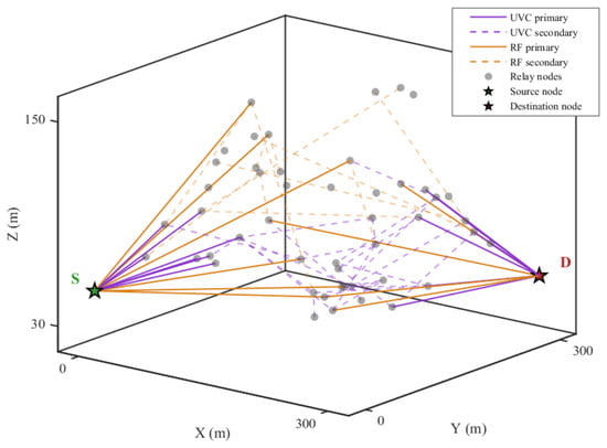
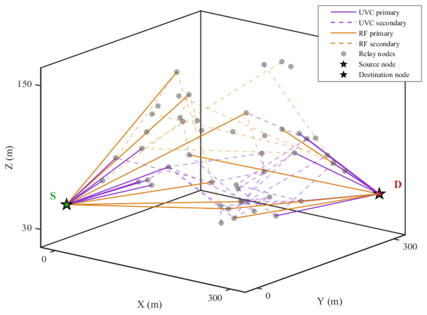
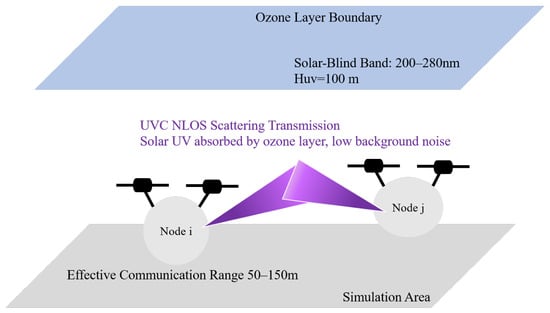
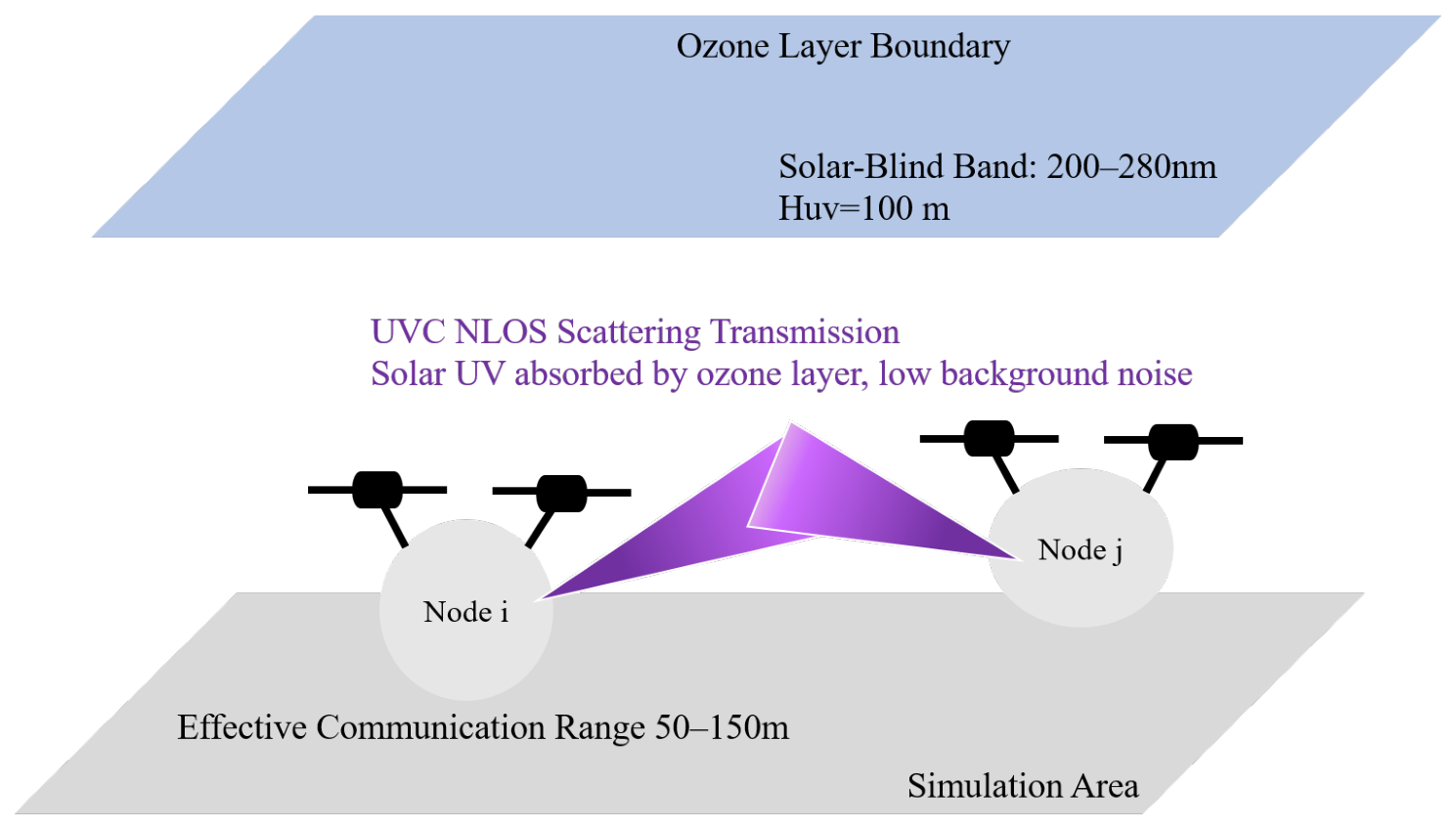
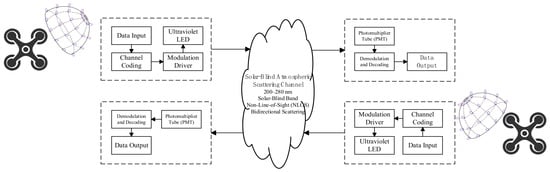
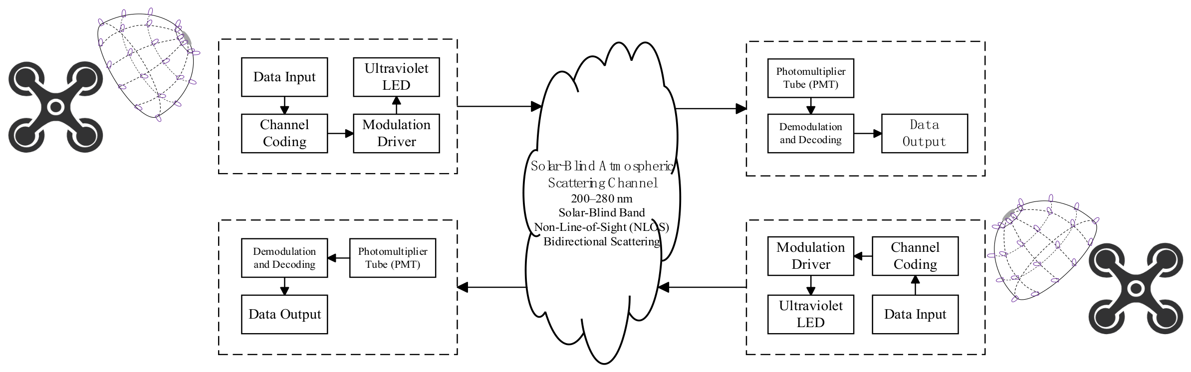
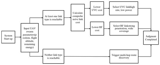
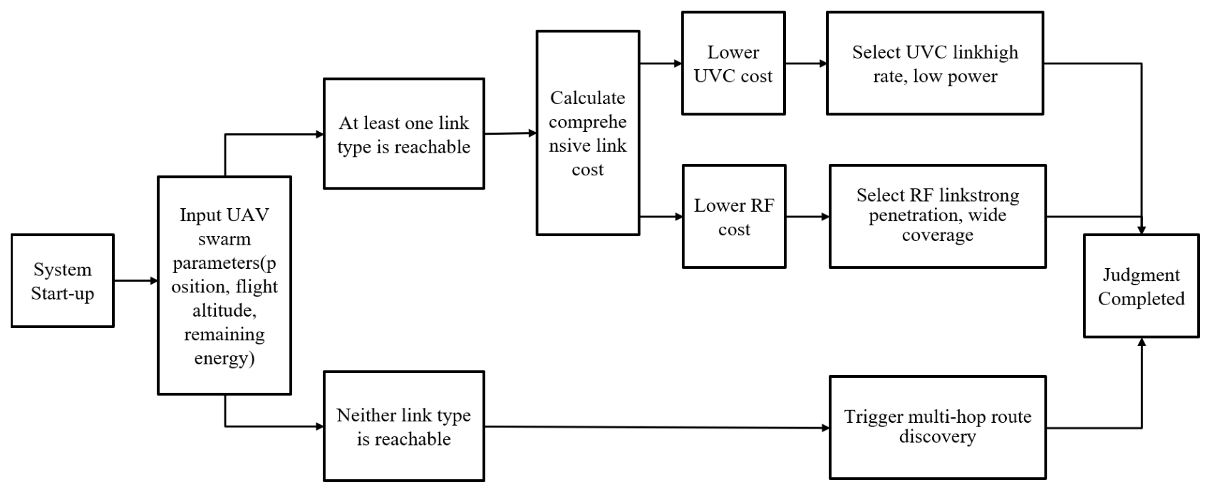
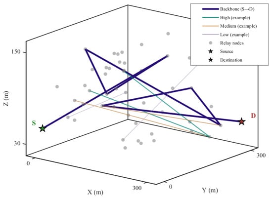
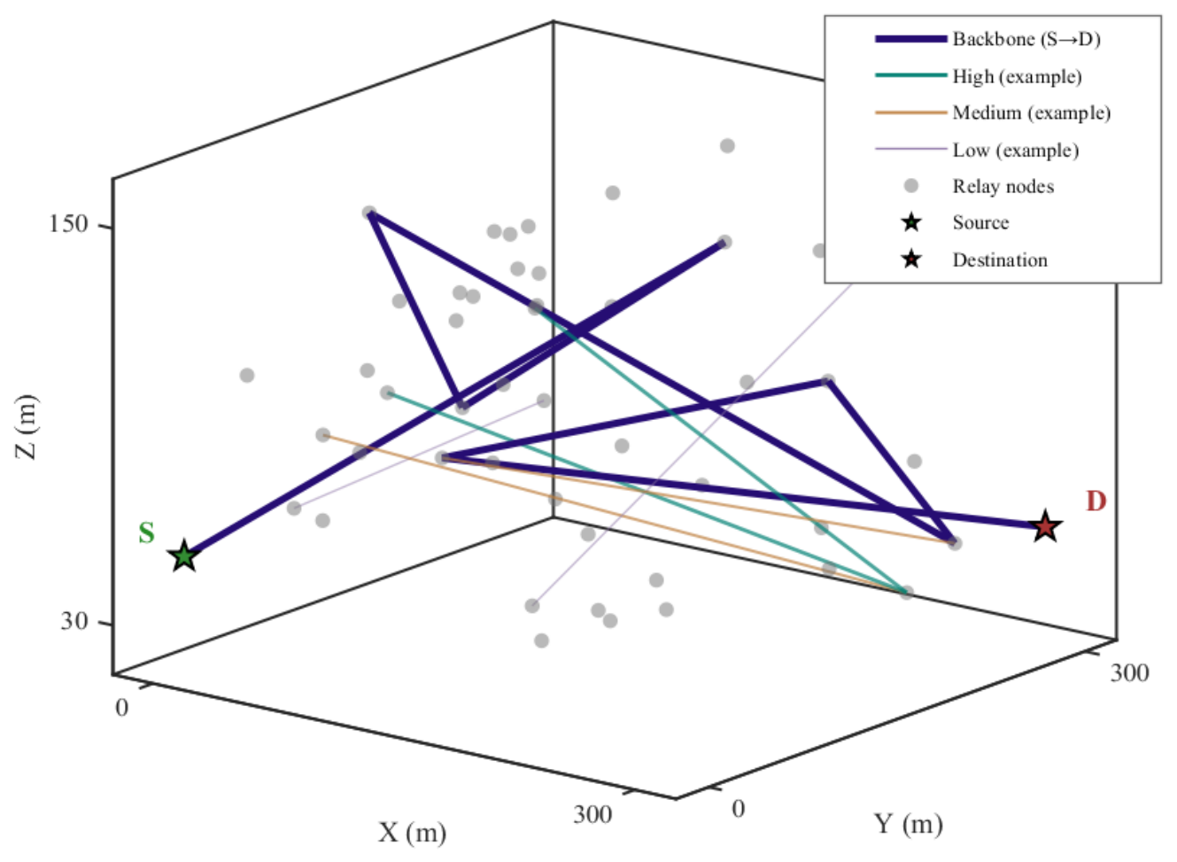
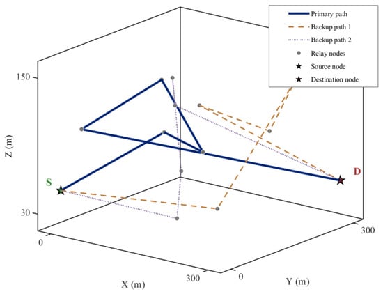
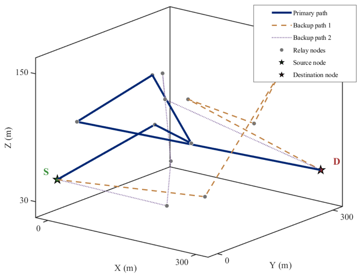
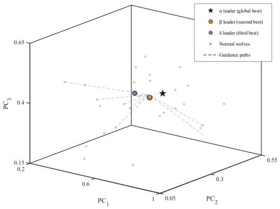
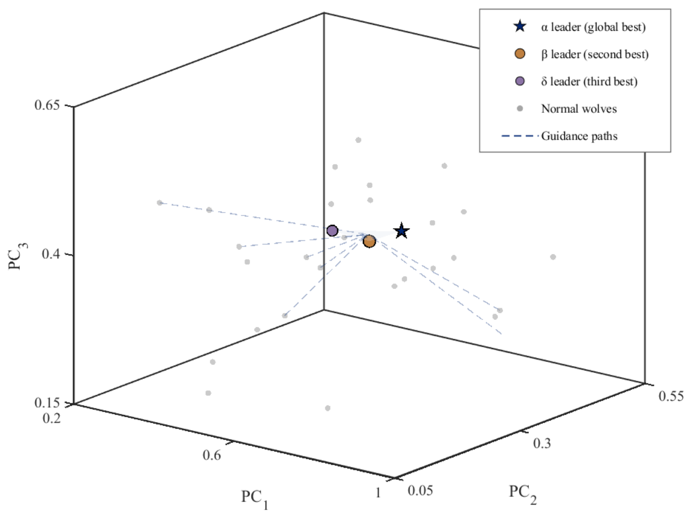
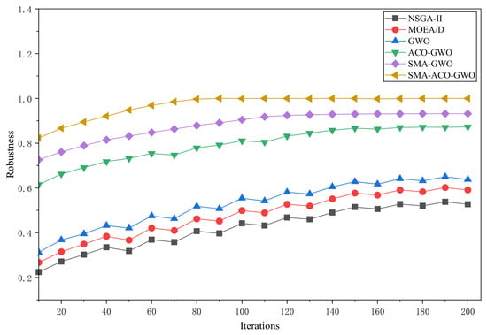
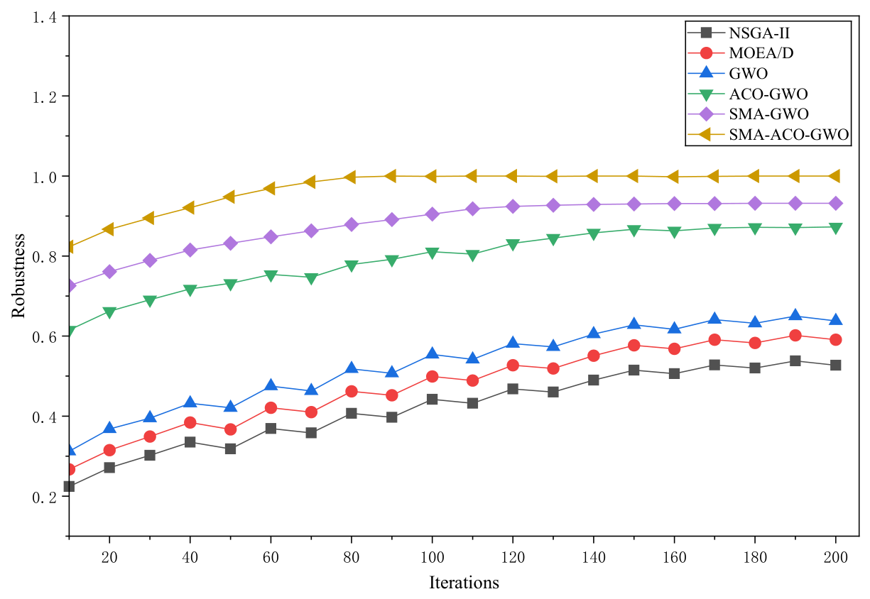
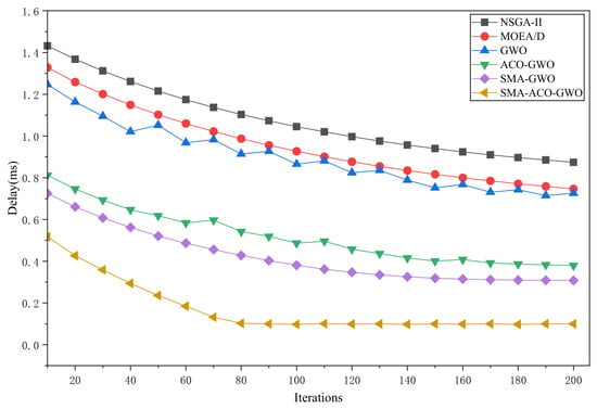
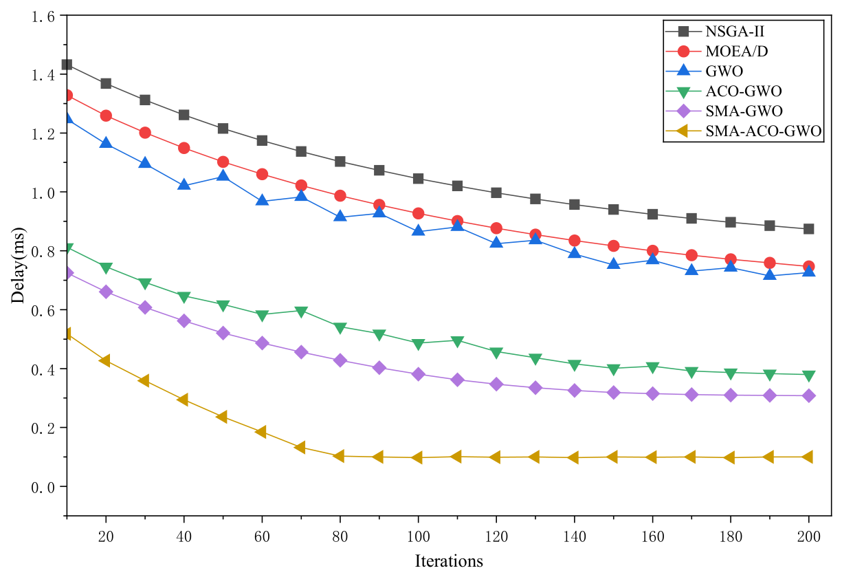
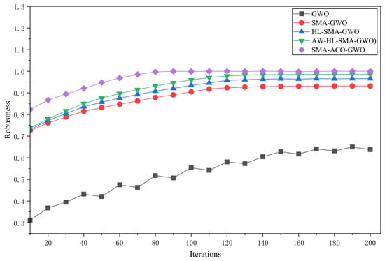
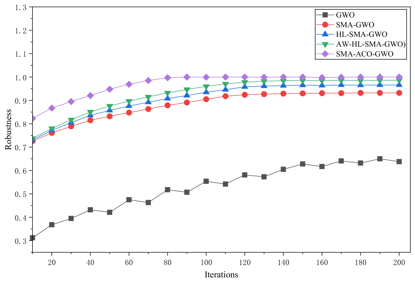
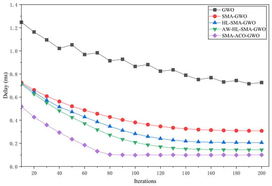
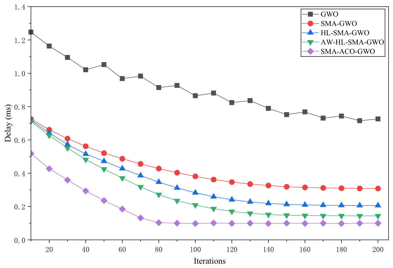
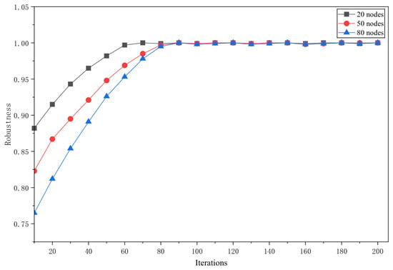
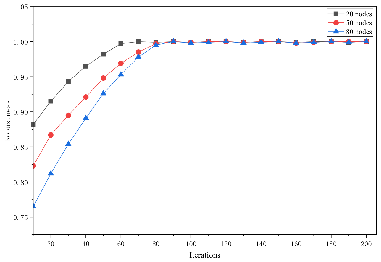
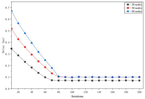
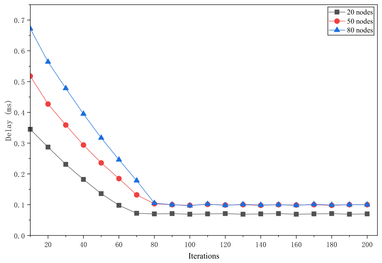
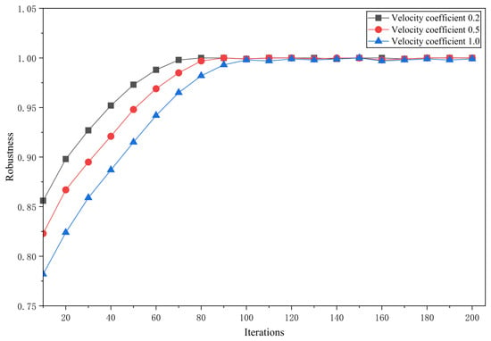
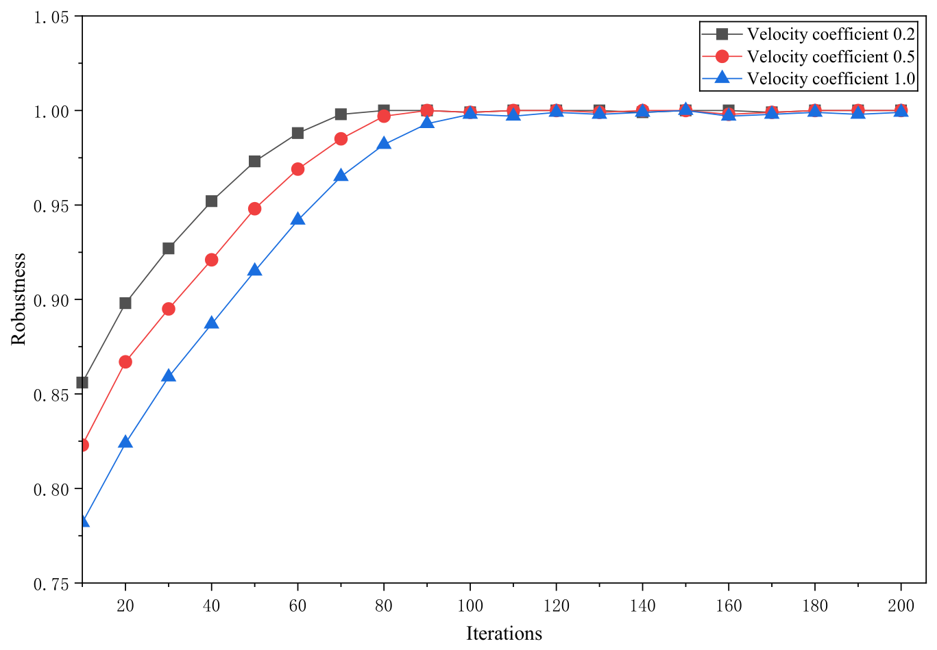
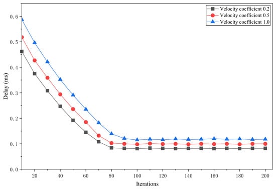
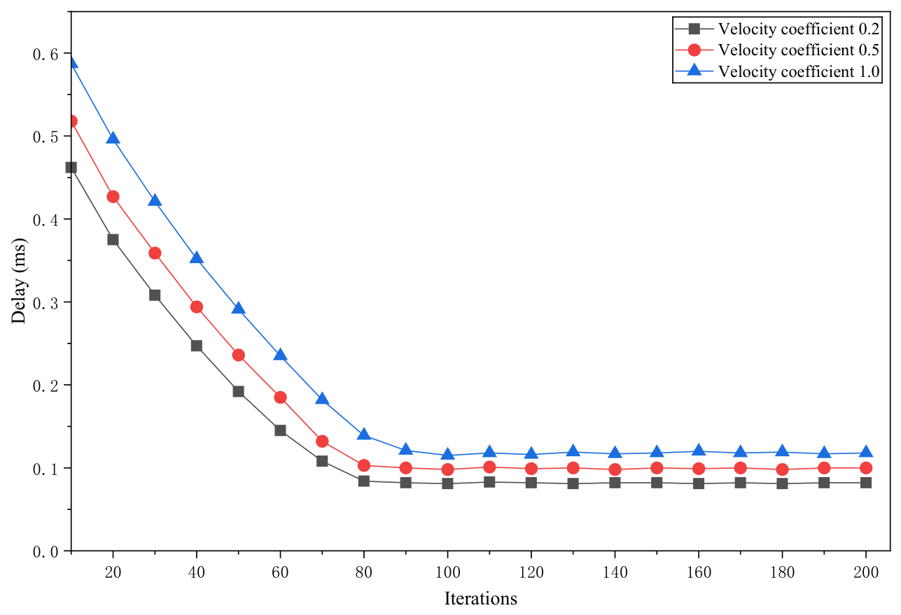
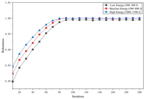
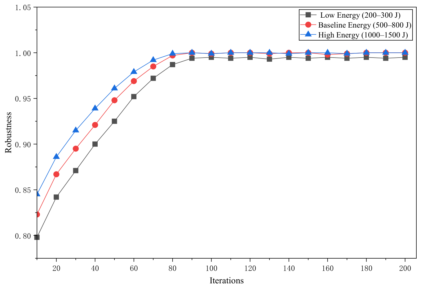
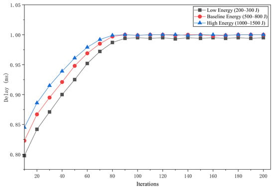
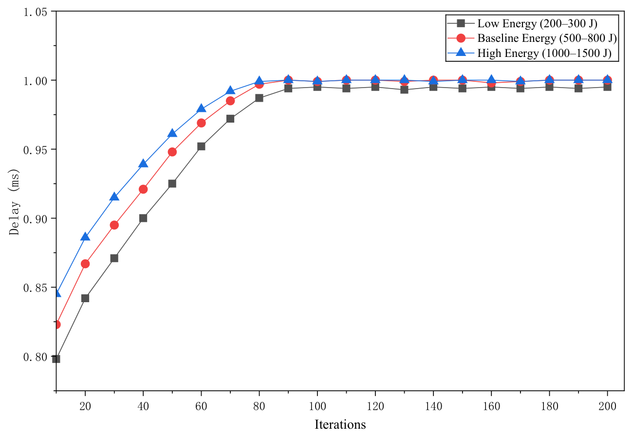

Disclaimer/Publisher’s Note: The statements, opinions and data contained in all publications are solely those of the individual author(s) and contributor(s) and not of MDPI and/or the editor(s). MDPI and/or the editor(s) disclaim responsibility for any injury to people or property resulting from any ideas, methods, instructions or products referred to in the content. |
© 2026 by the authors. Licensee MDPI, Basel, Switzerland. This article is an open access article distributed under the terms and conditions of the Creative Commons Attribution (CC BY) license.