Real-Time Thermal Human Activity Recognition on a CPU-Only Raspberry Pi 5 Using YOLO-Pose and Temporal Models

Abstract

Deploying human pose estimation and activity recognition on low-cost, accelerator-free hardware remains challenging, particularly for thermal imaging, which supports privacy-preserving and illumination-robust monitoring but has received comparatively little attention on CPU-only edge platforms. This study presents a complete thermal activity recognition pipeline that acquires video over RTSP, estimates human pose using YOLO-pose, and classifies six activities using lightweight temporal models, evaluated entirely on a Raspberry Pi 5 without a dedicated neural-network accelerator. Using a purpose-built single-participant thermal dataset with manually annotated pose keypoints and activity labels, YOLOv8-pose, YOLO11-pose, and YOLO26-pose were benchmarked in nano and small variants across native PyTorch, ONNX, and NCNN export formats, with NCNN reducing inference time by up to 2.9× while also minimizing power consumption; the selected YOLO26n-pose/NCNN configuration achieved 92.6% mAP50–95 at approximately 86 ms per frame. Five temporal architectures (LSTM, GRU, Conv1D, Conv1D-GRU, and a compact Transformer encoder) were then systematically compared across network sizes and observation windows on held-out test recordings. Network size was found to be the dominant driver of recognition performance, and convolutional and hybrid convolutional-recurrent architectures provided the most favorable accuracy–latency trade-offs at the low-latency end, while the highest Macro F1-score of 0.879 was obtained by a GRU at a processing rate of 5.8 FPS, with processing latency below 0.7 s and window-dependent response latency of 1.2–4.7 s. These results indicate that real-time thermal activity recognition is feasible on CPU-only edge hardware through careful joint selection of export format and temporal architecture, within the single-participant, full-body-visibility setting evaluated here.

1. Introduction

Human activity recognition identifies human movements, postures, and interactions from visual or other sequential sensor data and is widely used for automated analysis of human behavior. These methods support applications such as assisted living and healthcare monitoring, industrial safety and transportation safety [1,2,3]. In these contexts, continuous activity monitoring supports the timely identification of changes in behavior and potentially dangerous events without requiring constant human supervision. However, practical applications require continuously acquired data to be processed with sufficient accuracy and low latency, motivating the development of real-time recognition methods suitable for deployment on edge computing platforms.

Processing activity data locally on an edge device can reduce communication latency, dependence on network connectivity, and the transmission of sensitive information to remote servers. These advantages are particularly relevant for continuous monitoring systems, in which video or sensor data must be processed as they are acquired. However, embedded platforms provide considerably fewer computational and memory resources than desktop workstations or dedicated GPU systems. Consequently, the real-time feasibility of an activity recognition system depends not only on recognition accuracy but also on inference latency, memory usage, power consumption, and the computational requirements of the complete processing pipeline [1,3,4].

Vision-based activity recognition is commonly performed using RGB cameras, which provide detailed information about human appearance, surrounding objects, and environmental context. However, RGB cameras capture identity-revealing appearance information, and their performance can be affected by insufficient or varying illumination. Thermal imaging provides an alternative sensing modality by representing the thermal radiation emitted by people and surrounding objects rather than visual texture. Consequently, thermal data can support activity recognition in low-light or dark environments while limiting the amount of identifiable appearance information captured during continuous monitoring [5,6,7,8]. These characteristics make thermal imaging suitable for assisted living, indoor monitoring, and other privacy-sensitive applications.

Despite these advantages, thermal imagery presents several challenges for computer vision methods. Unlike RGB images, thermal images do not contain color information and generally provide less texture and spatial detail. The visibility and separability of individual body parts can also be affected by sensor resolution, thermal contrast, environmental temperature, occlusion, and thermally reflective surfaces. These factors can reduce the reliability of person detection and body keypoint estimation, particularly for small or partially occluded subjects [7,9,10]. These challenges are compounded by the limited availability of large thermal datasets containing reliable body keypoint annotations. Previous studies have therefore adapted pose-estimation models to thermal imagery using paired RGB and thermal recordings, knowledge transfer, automatically generated annotations, and domain-specific model training [5,9,11].

Once body keypoints have been detected, pose-based features provide an intermediate representation between thermal image acquisition and activity classification. Instead of supplying complete image sequences to the activity classifier, each detected person is represented using the coordinates and confidence values of anatomical keypoints. This compact representation reduces input dimensionality and limits the influence of background appearance while preserving body configuration information that can subsequently be analyzed over time. Thermal pose estimation has been investigated using bottom-up and top-down methods, lightweight convolutional architectures, and recent YOLO-pose models [5,6,12,13]. The keypoints detected in consecutive frames can then be arranged into temporal sequences and processed using recurrent, convolutional, or attention-based models to distinguish activities that cannot be identified reliably from an individual frame [14,15,16].

Recent studies have further examined the integration of thermal pose estimation into embedded monitoring systems. Lightweight thermal pose models have been deployed on embedded platforms, demonstrating the feasibility of performing pose estimation using compact and low-power computing hardware [11]. More comprehensive frameworks have combined thermal person detection, pose estimation, tracking, and contextual analysis, while other systems have evaluated thermal mobility recognition directly on low-cost edge devices [8,10]. However, previous studies have generally evaluated thermal pose estimation, temporal activity classification, or edge deployment as separate components. Consequently, limited evidence is available on complete thermal pose-based activity recognition pipelines operating on CPU-only single-board computers. In particular, the combined effects of pose-model family and export format, temporal architecture and network size, observation window, and sampling rate on recognition performance and computational cost remain insufficiently characterized under a common experimental protocol.

To address these challenges, this study develops and evaluates a thermal pose-based activity recognition pipeline on a CPU-only Raspberry Pi 5. The proposed pipeline receives thermal video through an RTSP stream, extracts human body keypoints using YOLO-pose, constructs temporal pose sequences, and classifies six human activities using lightweight temporal models. The evaluation considers pose-estimation accuracy, latency, and power consumption together with temporal activity-recognition performance, processing latency, and throughput under deployment-realistic conditions. This study builds on two earlier papers that used the same thermal pose dataset: ref. [17] evaluated YOLOv8-pose and YOLO11-pose on NVIDIA Jetson platforms, and ref. [18] investigated accuracy–efficiency trade-offs of thermal pose estimation on the Raspberry Pi 5. Both papers address pose estimation only. The present paper addresses the subsequent stage, i.e., recognizing activities from the estimated pose sequences, together with the complete deployed pipeline. The pose-estimation benchmark in Section 4.1 is therefore not claimed as a contribution; it is summarized to justify the choice of the pose front end and to report its latency and power consumption within the complete pipeline. The main contributions of this study are as follows:

• A multi-label thermal activity dataset of 93,070 annotated frames (approximately 62 min; 102,586 frames including background frames without a person) from 31 recordings, with six activity classes aligned with 17-keypoint pose information, made publicly available;
• A complete CPU-only pipeline (RTSP acquisition, YOLO-pose, temporal pose-sequence construction, activity classification) on a Raspberry Pi 5, with an explicit operational definition of real-time operation and a latency model that separates camera, pose-estimation and temporal-model delays;
• A systematic comparison of five temporal architectures, six network sizes and four observation windows under recording-level train/validation/test splits and five random seeds, with a Pareto analysis on measured Raspberry Pi 5 latency and a seed-aware ranking showing that the best configurations cannot be separated by Macro F1;
• The selection of the pose front end for this pipeline, building on [17,18]: YOLO26n-pose in NCNN format is chosen from the compared model families and export formats.

The remainder of this paper is organized as follows. Section 2 reviews human activity recognition methods and their deployment on Raspberry Pi platforms. Section 3 describes the materials and methods: the thermal pose and activity datasets (Section 3.1), the five temporal architectures (Section 3.2), the Raspberry Pi 5 platform (Section 3.3), the automated benchmarking protocol (Section 3.4) and the pose-estimation evaluation (Section 3.5). Section 4 presents the results on pose estimation (Section 4.1), action classification (Section 4.2) and end-to-end throughput, latency and the definition of real-time operation (Section 4.3). Section 5 discusses the findings and limitations, and Section 6 concludes the paper and outlines future work.

2. Related Works

Human activity recognition has been investigated using a wide range of input representations and temporal modeling approaches. Existing methods use RGB and infrared imagery, skeletal keypoints, and multi-modal sensor data together with recurrent, convolutional, attention-based, and transformer-based models. Alongside recognition accuracy, their practical application depends on the ability to operate within the computational constraints of low-cost edge devices. This section reviews recent human activity recognition methods and their deployment on Raspberry Pi platforms.

2.1. Human Activity Recognition Methods

Human activity recognition methods differ primarily in how human appearance, posture, and motion are represented for classification. Pose-based approaches use detected body keypoints, whereas other methods learn compact representations directly from video sequences or combine visual data with complementary sensor measurements. The selected representation determines how spatial and temporal information is encoded and provided to the activity-classification model.

A common strategy is to represent human motion as temporal sequences of body keypoints. Bharathi et al. [14] combined OpenPose with an attention-based LSTM network that processed 32 frame sequences of two dimensional skeletal coordinates. The method achieved an accuracy of 95.94% and an F1-score of 95.65% on six activities from the Berkeley Multimodal Human Action Database, considerably exceeding the accuracy of 73.18% obtained by a conventional LSTM. Similarly, Vijay et al. [19] combined body and hand landmarks extracted using MediaPipe with velocity, acceleration, and joint angle features. Their multibranch bidirectional LSTM model achieved an accuracy of 95.6% for eight indoor activities and processed RGB video at 43.5 FPS on a desktop CPU. Wang et al. [15] also used skeletal features extracted by LightOpenPose and evaluated several LSTM configurations with attention. Their lightweight model achieved an accuracy of 97.5% on a subset of the KTH dataset, while a double LSTM with attention achieved an accuracy of 96.3% for four occupant thermal adaptation activities.

Transformers and attention mechanisms have also been applied to model longer temporal relationships between successive poses. Sykes [16] compared OpenPose, PoseNet, and MediaPipe as pose extraction methods combined with transformer classifiers for fall detection. The MediaPipe configuration provided the best results, achieving an accuracy of 98% and an F1-score of 90.91%. For activity recognition under poor illumination, Luo et al. [20] proposed LPAC Net, in which Zero DCE++ image enhancement and YOLO Pose were combined with rotation invariant pose encoding and a bidirectional LSTM with multihead attention. The model achieved an accuracy of 95.53% and an F1-score of 94.9% on 12 activities from the ARID Fall dataset. However, the authors reported reduced reliability under extremely low illumination, severe occlusion, interactions involving multiple people, and inaccurate pose estimation.

Beyond skeleton-based representations, activity recognition can be performed using compact features learned directly from video sequences. Wanna et al. [21] proposed TinyAct, in which a lightweight video autoencoder transforms sequences of 16 RGB frames into latent representations that are subsequently classified using SVM, Random Forest, or XGBoost. Evaluation on the Kinetics 400 dataset showed that Random Forest achieved the highest accuracy of 57%, followed by SVM with 55% and XGBoost with 54%. These results demonstrate that compact latent representations can reduce the amount of transmitted data, although the recognition performance achieved on the evaluated dataset remained limited.

Infrared imaging provides an alternative representation when privacy or illumination conditions restrict the use of conventional RGB cameras. Park et al. [22] introduced the HDIA dataset containing 48 daily indoor activities recorded using infrared cameras and wearable armband sensors. Their infrared model achieved an accuracy of 86.41%, while the fusion of infrared, inertial, and electromyographic features increased the accuracy to 90.1%. Guo et al. [23] addressed the related task of posture detection in thermal images using adaptations of YOLOF, YOLOX, and TOOD. The best model achieved a composite mean average precision of 70.4% for standing, sitting, lying, and bending, with sitting and bending remaining more difficult because of occlusion, posture variation, and visual similarity.

Despite the generally high recognition results reported for pose-based and multimodal methods, their direct comparison remains difficult because of differences in activity classes, datasets, hardware, and evaluation protocols. The systematic review conducted by Nabizade et al. [24] similarly found that real-time fall detection studies frequently relied on small controlled datasets containing simulated falls and rarely included older participants. These findings indicate that recognition accuracy alone is insufficient for assessing practical applicability and that computational performance should also be evaluated directly on the intended deployment platform.

2.2. Deployment of Human Activity Recognition Methods on Raspberry Pi Platforms

Deploying human activity recognition methods on Raspberry Pi platforms requires recognition performance to be evaluated together with inference latency, memory usage, and power consumption. To support operation within these resource constraints, previous studies have used lightweight pose estimators, compact temporal models, model quantization, and optimized inference frameworks. The main characteristics and reported results are summarized in Table 1.

Table 1. Comparison of human activity recognition methods deployed on Raspberry Pi platforms.

Study	Raspberry Pi	Input	Resolution	Methods	Deployment Performance	Recognition Performance
Cho et al. [25]	Zero 2 W	RGB	Not specified	MediaPipe Pose, CNN, TCN, attention	325.88 ms per decision	Accuracy: 94.71% Macro F1-score: 93.63%
Huang et al. [26]	4	RGB	Not specified	YOLO-pose, bidirectional GRU, attention	8.3 FPS	Accuracy: 95.04% Macro F1-score: 94.3%
Le et al. [27]	4 Model B	RGB	$640\times 480$ px	Tiny HAR	2.8 ms classifier inference 1.32 s latency 2.6 W	Accuracy: 97.62% UR Falling dataset
Le et al. [28]	4 Model B	RGB	Not specified	MoveNet, TS ResCNN	12.2 ms classifier inference 2.8 W	Accuracy: 99.66% Florence 3D dataset
Sharma et al. [29]	4	RGB	$640\times 480$ px	MediaPipe Hands, quantized attention-based LSTM	500 ms per sequence 899 MB heap memory	Accuracy: 99.7% on the collected dataset Accuracy: 97.5% on CSLTR
Bach et al. [30]	3 Model B+	RGB	$640\times 640$ px	Optimized YOLOv8n-pose, LSTM	12.5 to 13.0 FPS 80 to 112 ms complete pipeline latency	Accuracy: 97% F1-score: 94%
Wang et al. [31]	4B	RGB	$254\times 192$ px	YOLOv7-tiny-pose, multi-branch 1D TCN	8.5 FPS	F1-score: 88%
Analia et al. [32]	5	Thermal	$256\times 192$ px	MediaPipe Pose, geometric features, KNN, SVC, MLP ensemble	0.2687 s average execution time per prediction	Accuracy: 98% F1-score: 98%

Note: Deployment values are reported according to the measurement scope used in each study. Some values represent classifier inference, whereas others represent decision latency or complete pipeline performance.

Pose-based fall and activity recognition on Raspberry Pi platforms has primarily relied on RGB cameras. Cho et al. [25] combined MediaPipe skeletal landmarks with a CNN, a temporal convolutional network, and an attention module. The method achieved an accuracy of 94.71% and a macro F1-score of 93.63%, while ONNX Runtime deployment on a Raspberry Pi Zero 2 W resulted in a decision latency of 325.88 ms. Huang et al. [26] combined an improved YOLO Pose model with a bidirectional GRU and attention mechanism for industrial activity recognition. The method achieved an accuracy of 95.04%, but its processing speed decreased from 48 FPS on GPU hardware to 8.3 FPS on a Raspberry Pi 4, which was below the required rate of 24 FPS. Bach et al. [30] optimized YOLOv8n Pose and combined it with LSTM-based fall classification on a Raspberry Pi 3 Model B+. The complete system achieved an F1-score of 94% and processed video at 12.5 to 13.0 FPS. However, fall detection performance decreased considerably under dim illumination, occlusion, and the presence of additional people.

System-level optimizations can further improve the performance of pose-based recognition pipelines. Wang et al. [31] combined YOLOv7 Tiny Pose with a multi-branch temporal convolutional network for monitoring people on a Raspberry Pi 4B. Motion-dependent frame skipping, adaptive keypoint selection, asynchronous processing, ONNX deployment, and INT8 quantization increased the processing speed from 6.1 to 8.5 FPS while maintaining an F1-score of 88%. Analia et al. [32] instead used thermal video to support privacy-preserving fall and prolonged immobility detection on a Raspberry Pi 5. MediaPipe Pose features were classified using a soft voting ensemble of KNN, SVC, and MLP models, producing an accuracy and F1-score of 98%. However, the evaluation was based on simulated falls performed by healthy participants, while severe occlusion and lateral body orientations reduced the reliability of thermal keypoint extraction.

Other studies have focused on reducing the complexity of skeletal sequence classification. Le et al. [27] deployed Tiny HAR using TensorFlow Lite on a Raspberry Pi 4 Model B. The classifier processed skeletal sequences of 35 frames in 2.8 ms and consumed approximately 2.6 W, while the reported system latency was 1.32 s. In a related study, Le et al. [28] evaluated TS ResCNN on the same platform using joint coordinates, pairwise distances, and several motion features within a compact residual convolutional architecture. The classifier required 12.2 ms per sequence and consumed approximately 2.8 W when integrated with MoveNet pose estimation. For dynamic sign language recognition, Sharma et al. [29] deployed a quantized attention-based LSTM using MediaPipe hand landmarks on a Raspberry Pi 4. The model achieved accuracies of 99.7% and 97.5% on two datasets, but required approximately 500 ms to classify a gesture sequence and used 899 MB of heap memory.

The reviewed studies show that skeletal representations and temporal models can support accurate activity recognition, while infrared sensing is suitable for applications in which privacy and illumination are important considerations. Nevertheless, recognition performance remains sensitive to dataset composition, pose-estimation quality, occlusion, viewpoint, and sensing conditions. Raspberry Pi deployments demonstrate the feasibility of local activity recognition using lightweight models, quantization, and optimized inference frameworks. However, direct comparison remains difficult because the reported measurements may represent classifier inference time, complete pipeline latency, or application-level throughput. Most reviewed implementations use RGB video, and several focus specifically on fall detection, whereas complete thermal activity recognition pipelines on Raspberry Pi platforms remain limited. Existing work also provides limited comparison of YOLO-pose families, export formats, temporal architectures, and sampling conditions under a common experimental protocol. Therefore, the combined setting of thermal imagery, pose-based temporal recognition, and CPU-only Raspberry Pi 5 deployment remains underexplored, particularly when pose accuracy and power consumption are considered together with activity-recognition performance, latency, and throughput.

3. Materials and Methods

3.1. Thermal Image and Activity Datasets

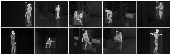
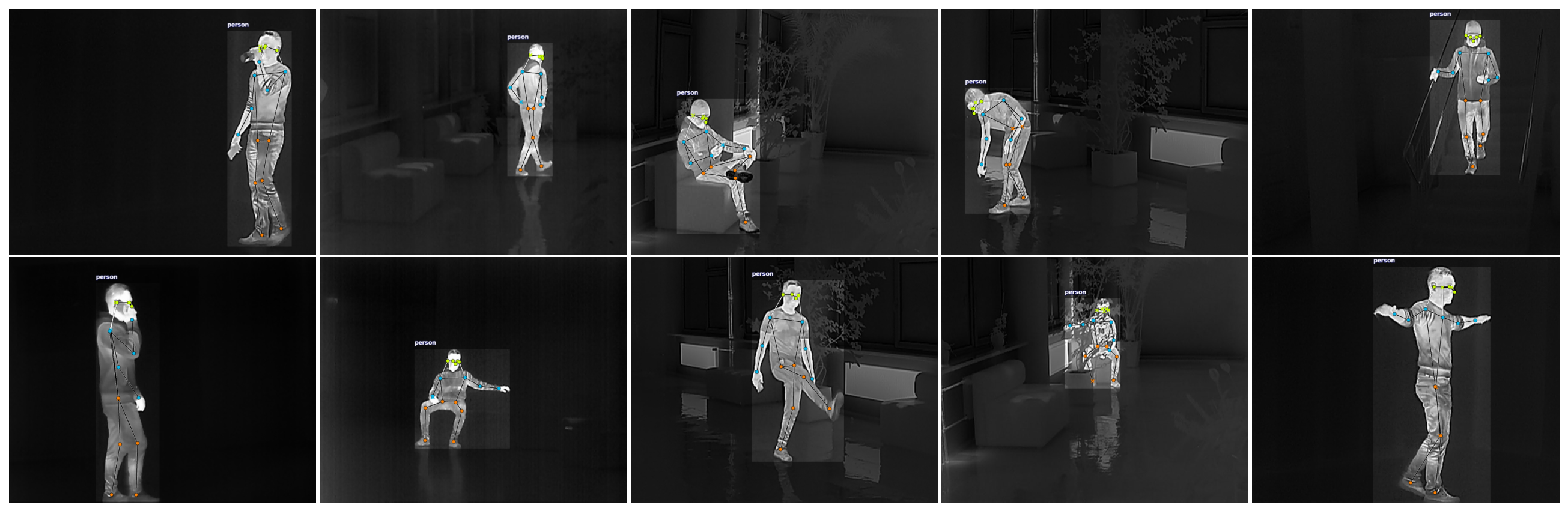
A single-person thermal image dataset was collected to evaluate human pose estimation under the intended edge-deployment conditions. Thermal video was captured using a Lynx L15 thermal monocular (HIKMICRO, Hangzhou, China) at a spatial resolution of $720\times 576$ px and a frame rate of 25 FPS, with the recordings stored as MP4 video sequences. To reduce redundancy between temporally adjacent frames during pose annotation, every fifth frame was sampled from the original recordings. The resulting dataset contained 2500 manually annotated thermal frames, with each frame labeled using a single-person bounding box and 17 body keypoints following the standard human pose estimation annotation format (Figure 1).

Figure 1. Representative thermal images from the dataset showing the 17 manually annotated human pose keypoints.

The dataset was collected from a single male participant of average build. To introduce variation in the observed thermal silhouette, self-occlusion, and body-heat distribution, three clothing conditions were used during recording: a T-shirt, a sweater, and a jacket worn with a hat. Recordings were performed in eight different indoor rooms at an ambient temperature of approximately 21 °C. The different recording environments introduced variation in background clutter, furniture arrangement, and thermally reflective surfaces while keeping the participant and thermal camera model fixed.

The thermal image dataset and the corresponding training splits are the same as those used in our previous study of embedded GPU deployment on Jetson platforms [17]. In that study, YOLOv8-pose and YOLO11-pose model families were evaluated on NVIDIA Jetson Orin Nano and AGX Orin platforms using TensorRT with FP32, FP16, and INT8 precision. The present work extends this evaluation to the complementary accelerator-free setting of CPU-only inference on the Raspberry Pi 5. The same thermal pose data are therefore used to train the pose-estimation models, while the present study additionally evaluates YOLO26-pose and investigates CPU-oriented export formats, namely native PyTorch, ONNX, and NCNN.

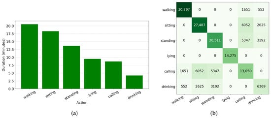
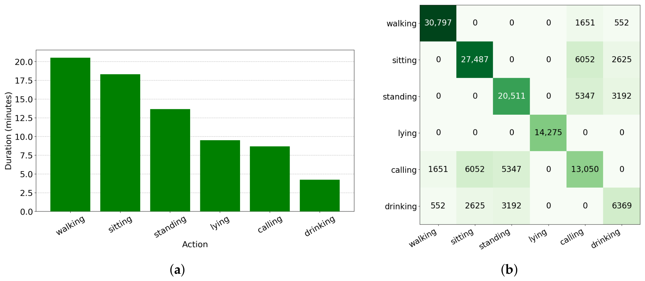
For temporal human activity recognition, an annotated action dataset was constructed automatically from the thermal video recordings applying the YOLO26x-pose in native PyTorch format, the most accurate model in [18] (pose mAP50–95 of 95.6%), trained on the 2000 training frames of the annotated pose dataset. The dataset contains six activity classes: walking, sitting, standing, lying, calling, and drinking. In total, the action dataset contains 93,070 annotated frames corresponding to approximately 62 min of activity recordings at 25 FPS (102,586 frames in total covering background frames without person). The walking class contains 30,797 frames (20.5 min), sitting contains 27,487 frames (18.3 min), standing contains 20,511 frames (13.7 min), lying contains 14,275 frames (9.5 min), calling contains 13,050 frames (8.7 min), and drinking contains 6369 frames (4.2 min). Activities can occur simultaneously: walking, sitting, or standing may be combined with calling or drinking, so a frame may carry two active labels. Approximately 21% of the annotated frames have two labels, whereas lying was never combined with another class and calling and drinking were never annotated alone (Figure 2b). The class-wise frame counts therefore overlap, and their sum (112,489 frames) exceeds the number of annotated frames. In Figure 2a, frames with two active labels are counted in both classes; in Figure 2b, the diagonal cells give the total number of frames per class and the off-diagonal cells give the number of frames in which two activities are active simultaneously.

Figure 2. Distribution of activity classes: (a) duration of each class; (b) co-occurrence matrix of activity labels.

Each action annotation is stored together with the pose information for the corresponding frame. The annotation record follows the structure:

$$[frame, walking, sitting, standing, lying, calling, drinking, {kp}_{1x}, {kp}_{1y}, {kp}_{1v}, \dots , {kp}_{17v}],$$

where the first field identifies the video frame, the following six fields contain the activity labels, and each of the 17 keypoints is represented by its horizontal coordinate, vertical coordinate, and predicted confidence. The six activity labels are encoded as independent binary values (a multi-hot vector), so that several labels can be active in the same frame, allowing the action-recognition models to produce an independent probability for each activity class. The participant was fully visible in the image during all activities, so that all 17 keypoints were within the field of view. Frontal, lateral and oblique orientations occur during walking, standing, sitting, calling and drinking.

Before temporal model training, the spatial keypoint coordinates were converted to bounding-box-relative coordinates. Specifically, the horizontal and vertical keypoint locations were normalized with respect to the width and height of the person’s bounding box, respectively. This representation reduces the influence of the person’s absolute image location and scale while retaining the relative spatial configuration of the body. The resulting pose representation contains 17 keypoints with three values per keypoint, giving $17\times 3=51$ input features per frame. Consequently, each temporal sample supplied to the action-recognition models is represented as a sequence $\mathrm{X}\in {\mathbb{R}}^{T\times 51}$, where T is determined by the selected temporal observation window and video sampling rate.

The original action recordings were acquired at 25 FPS. For temporal sequence construction, the recordings were decimated by a factor of four to approximately 6 FPS, which corresponds to the throughput sustained by the complete deployed pipeline on the Raspberry Pi 5. The resulting pose sequences were used as input to the LSTM, GRU, Conv1D, Conv1D-GRU, and Transformer-based temporal classifiers.

3.2. Temporal Models

Five lightweight temporal architectures were evaluated for action classification from pose sequences: LSTM, GRU, Conv1D, Conv1D-GRU, and a compact Transformer encoder. All models receive a temporal sequence of pose features as input and produce independent probabilities for the six activity classes using a sigmoid output layer. The input sequence is represented as $\mathrm{X}\in {\mathbb{R}}^{T\times D}$, where T denotes the sequence length and $D=51$ denotes the number of input features obtained from 17 pose keypoints, each represented by its horizontal coordinate, vertical coordinate, and confidence value. Across all five architectures, the network-size parameter N denotes the number of units in recurrent and dense layers and the number of filters in convolutional layers, and a dropout rate of 0.2 is applied consistently after each recurrent, convolutional, or dense block.

The LSTM architecture consists of two stacked bidirectional LSTM layers. The first layer returns the complete sequence so that the second recurrent layer can process the resulting temporal representation. Dropout is applied between the recurrent layers, followed by a fully connected layer, a second dropout layer, and a six-unit sigmoid output layer. The corresponding architecture is summarized in Algorithm 1.

Algorithm 1 Bidirectional LSTM architecture

Require:  Pose sequence $\mathrm{X}\in {\mathbb{R}}^{T\times D}$, number of units N Ensure:  Six-dimensional activity probability vector $\widehat{\mathrm{y}}$   1: ${\mathrm{H}}_1\leftarrow \mathrm{BiLSTM}(\mathrm{X},N,\mathrm{return}\_\mathrm{sequences}=\mathrm{True})$   2: ${\mathrm{H}}_1\leftarrow \mathrm{Dropout}({\mathrm{H}}_1,0.2)$   3: ${\mathrm{H}}_2\leftarrow \mathrm{BiLSTM}({\mathrm{H}}_1,N)$   4: $\mathrm{h}\leftarrow \mathrm{Dense}({\mathrm{H}}_2,N,\mathrm{ReLU})$   5: $\mathrm{h}\leftarrow \mathrm{Dropout}(\mathrm{h},0.2)$   6: $\widehat{\mathrm{y}}\leftarrow \mathrm{Dense}(\mathrm{h},6,\mathrm{Sigmoid})$   7: return  $\widehat{\mathrm{y}}$

The GRU model follows a similar stacked recurrent structure but uses two unidirectional GRU layers. The first GRU layer preserves the temporal dimension, while the second GRU layer produces the final sequence representation. A dense layer with ReLU activation and dropout forms the classification head before the six independent sigmoid outputs. This architecture is shown in Algorithm 2.

Algorithm 2 Stacked GRU architecture

Require:  Pose sequence $\mathrm{X}\in {\mathbb{R}}^{T\times D}$, number of units N Ensure:  Six-dimensional activity probability vector $\widehat{\mathrm{y}}$   1: ${\mathrm{H}}_1\leftarrow \mathrm{GRU}(\mathrm{X},N,\mathrm{return}\_\mathrm{sequences}=\mathrm{True})$   2: ${\mathrm{H}}_1\leftarrow \mathrm{Dropout}({\mathrm{H}}_1,0.2)$   3: ${\mathrm{H}}_2\leftarrow \mathrm{GRU}({\mathrm{H}}_1,N)$   4: $\mathrm{h}\leftarrow \mathrm{Dense}({\mathrm{H}}_2,N,\mathrm{ReLU})$   5: $\mathrm{h}\leftarrow \mathrm{Dropout}(\mathrm{h},0.2)$   6: $\widehat{\mathrm{y}}\leftarrow \mathrm{Dense}(\mathrm{h},6,\mathrm{Sigmoid})$   7: return  $\widehat{\mathrm{y}}$

The Conv1D architecture replaces recurrent processing with two temporal one-dimensional convolutional layers. Both convolutional layers use N filters, a kernel size of five, ReLU activation, and same padding. Dropout follows each convolutional layer. Global average pooling then aggregates the temporal representation before a dense classification layer and the final sigmoid output layer. This design provides local temporal feature extraction with a comparatively simple computational structure, as summarized in Algorithm 3.

Algorithm 3 Conv1D architecture

Require:  Pose sequence $\mathrm{X}\in {\mathbb{R}}^{T\times D}$, number of filters N Ensure:  Six-dimensional activity probability vector $\widehat{\mathrm{y}}$   1: ${\mathrm{H}}_1\leftarrow \mathrm{Conv}1\mathrm{D}(\mathrm{X},N,k=5,\mathrm{ReLU},\mathrm{same})$   2: ${\mathrm{H}}_1\leftarrow \mathrm{Dropout}({\mathrm{H}}_1,0.2)$   3: ${\mathrm{H}}_2\leftarrow \mathrm{Conv}1\mathrm{D}({\mathrm{H}}_1,N,k=5,\mathrm{ReLU},\mathrm{same})$   4: ${\mathrm{H}}_2\leftarrow \mathrm{Dropout}({\mathrm{H}}_2,0.2)$   5: $\mathrm{h}\leftarrow \mathrm{GlobalAveragePooling}1\mathrm{D}\left({\mathrm{H}}_2\right)$   6: $\mathrm{h}\leftarrow \mathrm{Dense}(\mathrm{h},N,\mathrm{ReLU})$   7: $\mathrm{h}\leftarrow \mathrm{Dropout}(\mathrm{h},0.2)$   8: $\widehat{\mathrm{y}}\leftarrow \mathrm{Dense}(\mathrm{h},6,\mathrm{Sigmoid})$   9: return  $\widehat{\mathrm{y}}$

The Conv1D-GRU architecture combines local temporal feature extraction with recurrent temporal modeling. Two Conv1D layers first extract short-range temporal patterns from the pose sequence, using the same kernel size and filter count as the standalone Conv1D architecture. The resulting feature sequence is then processed by a GRU layer, which models longer-range temporal dependencies. A dense layer, dropout, and sigmoid classification layer complete the architecture. The resulting sequence of operations is given in Algorithm 4.

Algorithm 4 Conv1D-GRU architecture

Require:  Pose sequence $\mathrm{X}\in {\mathbb{R}}^{T\times D}$, number of filters/units N Ensure:  Six-dimensional activity probability vector $\widehat{\mathrm{y}}$   1: ${\mathrm{H}}_1\leftarrow \mathrm{Conv}1\mathrm{D}(\mathrm{X},N,k=5,\mathrm{ReLU},\mathrm{same})$   2: ${\mathrm{H}}_1\leftarrow \mathrm{Dropout}({\mathrm{H}}_1,0.2)$   3: ${\mathrm{H}}_2\leftarrow \mathrm{Conv}1\mathrm{D}({\mathrm{H}}_1,N,k=5,\mathrm{ReLU},\mathrm{same})$   4: ${\mathrm{H}}_2\leftarrow \mathrm{Dropout}({\mathrm{H}}_2,0.2)$   5: $\mathrm{h}\leftarrow \mathrm{GRU}({\mathrm{H}}_2,N)$   6: $\mathrm{h}\leftarrow \mathrm{Dense}(\mathrm{h},N,\mathrm{ReLU})$   7: $\mathrm{h}\leftarrow \mathrm{Dropout}(\mathrm{h},0.2)$   8: $\widehat{\mathrm{y}}\leftarrow \mathrm{Dense}(\mathrm{h},6,\mathrm{Sigmoid})$   9: return  $\widehat{\mathrm{y}}$

A compact Transformer encoder was evaluated to provide attention-based temporal modeling. The input features are first projected to the dense dimension $N_D$. A multi-head self-attention block with four attention heads and a key dimension of 16 models temporal relationships between observations. The attention output is combined with the input through a residual connection followed by layer normalization. A two-layer feed-forward network with an intermediate dimension of $2N_D$ is then applied, again followed by a residual connection and layer normalization. Global average pooling aggregates the temporal representation before the final dense classification head. The architecture is summarized in Algorithm 5.

Algorithm 5 Compact Transformer encoder architecture

Require:  Pose sequence $\mathrm{X}\in {\mathbb{R}}^{T\times D}$, dense dimension $N_D$ Ensure:  Six-dimensional activity probability vector $\widehat{\mathrm{y}}$   1: $\mathrm{H}\leftarrow \mathrm{Dense}(\mathrm{X},N_D)$   2: $\mathrm{A}\leftarrow \mathrm{MultiHeadAttention}(\mathrm{H},\mathrm{H},h=4,k=16)$   3: $\mathrm{H}\leftarrow \mathrm{LayerNorm}(\mathrm{H}+\mathrm{A})$   4: $\mathrm{F}\leftarrow \mathrm{Dense}(\mathrm{H},2N_D,\mathrm{ReLU})$   5: $\mathrm{F}\leftarrow \mathrm{Dense}(\mathrm{F},N_D)$   6: $\mathrm{H}\leftarrow \mathrm{LayerNorm}(\mathrm{H}+\mathrm{F})$   7: $\mathrm{h}\leftarrow \mathrm{GlobalAveragePooling}1\mathrm{D}\left(\mathrm{H}\right)$   8: $\mathrm{h}\leftarrow \mathrm{Dense}(\mathrm{h},N_D,\mathrm{ReLU})$   9: $\mathrm{h}\leftarrow \mathrm{Dropout}(\mathrm{h},0.2)$ 10: $\widehat{\mathrm{y}}\leftarrow \mathrm{Dense}(\mathrm{h},6,\mathrm{Sigmoid})$ 11: return  $\widehat{\mathrm{y}}$

For all architectures, the six output neurons correspond to walking, sitting, standing, lying, calling, and drinking. A sigmoid activation was used because the classifier produces an independent probability for each activity class rather than a mutually exclusive one. Each sequence is assigned the multi-hot label vector $\mathrm{y}\in {\{0,1\}}^6$ of its last frame, and the network is trained with binary cross-entropy applied to each output. Each output is thresholded independently, ${\widehat{y}}_c=\mathbb{1}[p_c>0.5]$, without softmax or argmax, so that concurrent activities (e.g., standing and calling) are predicted simultaneously, and a sequence may also receive a single label or no label. During evaluation, an activity was considered positive when its predicted probability exceeded the fixed threshold of 0.5. The recurrent, convolutional, and attention-based architectures were evaluated using the same experimental protocol, including the shared dropout rate and network-size parameter N, allowing their recognition performance and computational characteristics to be compared under equivalent conditions.

Each architecture is described step by step below; the step numbers correspond to the line numbers of the respective algorithm. Tensor shapes are given per sample (batch dimension omitted), where T is the sequence length, $D=51$ the number of input features and N the network-size parameter.

Bidirectional LSTM (Algorithm 1):

Step 1.

The first BiLSTM layer reads $\mathrm{X}\in {\mathbb{R}}^{T\times D}$ forwards and backwards with N units per direction and returns the output of every time step, ${\mathrm{H}}_1\in {\mathbb{R}}^{T\times 2N}$.

Step 2.

Dropout (0.2) is applied to ${\mathrm{H}}_1$.

Step 3.

The second BiLSTM layer processes this sequence and returns only its final output, which condenses the window into one vector ${\mathrm{H}}_2\in {\mathbb{R}}^{2N}$.

Step 4.

A dense layer with N units and ReLU activation gives $\mathrm{h}\in {\mathbb{R}}^N$.

Step 5.

Dropout (0.2) is applied to $\mathrm{h}$.

Step 6.

A dense layer with six units and sigmoid activation outputs the independent probabilities of the six activities, $\widehat{\mathrm{y}}\in {[0,1]}^6$.

In the stacked GRU (Algorithm 2), Steps 1–6 are identical, except that both GRU layers are unidirectional; hence ${\mathrm{H}}_1\in {\mathbb{R}}^{T\times N}$ and ${\mathrm{H}}_2\in {\mathbb{R}}^N$.

The Conv1D (Algorithm 3):

Step 1.

A one-dimensional convolution with N filters, kernel size five, ReLU activation and same padding is applied along time, giving ${\mathrm{H}}_1\in {\mathbb{R}}^{T\times N}$; each output step depends on five consecutive frames.

Step 2.

Dropout (0.2) is applied.

Step 3.

A second identical convolution gives ${\mathrm{H}}_2\in {\mathbb{R}}^{T\times N}$ (receptive field of nine frames).

Step 4.

Dropout (0.2) is applied.

Step 5.

Global average pooling averages ${\mathrm{H}}_2$ over time, giving $\mathrm{h}\in {\mathbb{R}}^N$ independently of T.

Step 6.

A dense layer with N units and ReLU activation follows.

Step 7.

Dropout (0.2) is applied.

Step 8.

The six-unit sigmoid layer outputs $\widehat{\mathrm{y}}\in {[0,1]}^6$.

In the Conv1D-GRU (Algorithm 4), Steps 1–4 are identical to Conv1D. In Step 5 a GRU layer with N units reads the feature sequence ${\mathrm{H}}_2$ in temporal order and returns its final state $\mathrm{h}\in {\mathbb{R}}^N$ instead of global average pooling; Steps 6–8 are identical to Conv1D.

The Transformer encoder (Algorithm 5): Here $N_D=N$.

Step 1.

A dense layer projects the 51 features of each frame to $N_D$ dimensions, $\mathrm{H}\in {\mathbb{R}}^{T\times N_D}$.

Step 2.

Multi-head self-attention (four heads, key dimension 16) lets every frame attend to all frames of the window, giving $\mathrm{A}\in {\mathbb{R}}^{T\times N_D}$.

Step 3.

The residual sum $\mathrm{H}+\mathrm{A}$ is layer-normalized and replaces $\mathrm{H}$.

Step 4.

A position-wise feed-forward network is applied to every time step: a dense layer with $2N_D$ units and ReLU activation.

Step 5.

The second dense is applied layer with $N_D$ units, giving $\mathrm{F}\in {\mathbb{R}}^{T\times N_D}$.

Step 6.

The residual sum $\mathrm{H}+\mathrm{F}$ is layer-normalized and replaces $\mathrm{H}$.

Step 7.

Global average pooling over time gives $\mathrm{h}\in {\mathbb{R}}^{N_D}$.

Step 8.

A dense layer with $N_D$ units and ReLU activation follows.

Step 9.

Dropout (0.2) is applied.

Step 10.

The six-unit sigmoid layer outputs $\widehat{\mathrm{y}}\in {[0,1]}^6$.

3.3. Edge Deployment Platform

The trained models were deployed and benchmarked on a Raspberry Pi 5 Model B (Rev. 1.1; Raspberry Pi Ltd., Cambridge, UK) single-board computer, a CPU-centric edge platform based on the Broadcom BCM2712 system-on-chip with a quad-core Arm Cortex-A76 processor (Arm Ltd., Cambridge, UK) running at up to 2.4 GHz and 8 GB of LPDDR4X RAM. The Raspberry Pi 5 was operated with 64-bit Raspberry Pi OS (release XX, based on Debian GNU/Linux 13.4 “trixie”) and relied exclusively on its CPU for neural-network inference, without a dedicated GPU, NPU, or other neural-network accelerator. The overall deployment architecture is illustrated in Figure 3.

Figure 3. Structural representation of deployment architecture.

Thermal video was acquired using a Lynx L15 thermal monocular, which provided a Wi-Fi hotspot and an RTSP video stream. The Raspberry Pi 5 connected directly to this wireless network and received the thermal video through the RTSP interface. The RTSP stream was supplied directly to the YOLO-pose inference pipeline, eliminating the need for intermediate video-file transfer during real-time operation. The pipeline processes the most recent frame of the stream and discards frames that arrive during processing. The detected human keypoints were subsequently passed to the temporal action-recognition model for activity classification. Thus, the deployed pipeline consisted of thermal image acquisition, RTSP streaming, pose estimation, temporal pose-sequence construction, and action classification.

The edge-deployment software stack consisted of Debian GNU/Linux 13.4 (trixie), Linux kernel 6.12.75+rpt-rpi-2712 (aarch64), Python 3.13.5, PyTorch 2.10.0 (CPU build), ONNX Runtime 1.24.4, NCNN (https://github.com/Tencent/ncnn, (accessed on 9 October 2026)), OpenCV 4.13.0, Ultralytics 8.4.23, TensorFlow 2.21.0, Keras 3.15.1, and NumPy 2.4.3. The YOLO-pose models were exported from native PyTorch to ONNX and NCNN formats using the Ultralytics export function. The YOLO-pose models received the RTSP stream as their input source and operated in inference mode using the Ultralytics/PyTorch/ONNX components of this stack, while the temporal action-recognition models were executed using TensorFlow/Keras. The resulting pose coordinates, confidence values, and temporal observations were then used by the trained action-recognition models running on the same Raspberry Pi 5.

The training and deployment environments were intentionally separated. Model training was performed on an NVIDIA GeForce RTX 4080 Super GPU, whereas the final inference experiments were performed using the CPU-only software environment on the Raspberry Pi 5. This separation ensures that the reported edge performance reflects the computational characteristics of the target deployment platform rather than those of the training workstation.

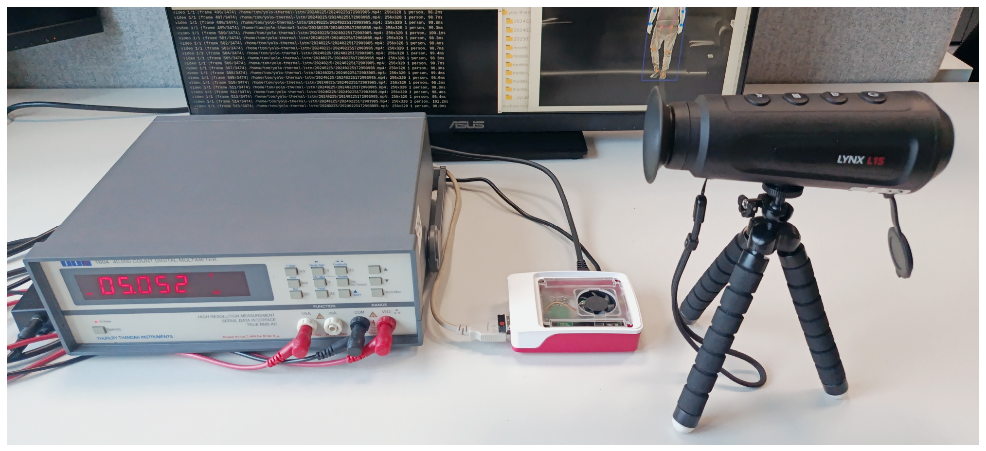
During benchmarking, the Raspberry Pi 5 used four CPU threads for the inference backends, corresponding to its four physical Cortex-A76 cores. The board used its integrated active cooling system without additional external cooling. The experimental setup used for evaluating real-time operation includes the Raspberry Pi 5, the Lynx L15 thermal monocular, and a TTi 1604 digital multimeter (Thurlby Thandar Instruments, Huntingdon, UK) for power logging (Figure 4).

Figure 4. Experimental setup for real-time evaluation on the Raspberry Pi 5.

3.4. Automated Benchmarking Protocol

An automated benchmarking script was developed to systematically evaluate the temporal action-recognition models under a common experimental protocol. Five architectures (LSTM, GRU, Conv1D, Conv1D-GRU, and Transformer encoder) were evaluated using six network sizes, $N\in \{8,16,32,64,128,256\}$, and four temporal windows of approximately 1, 2, 4, and 8 s. The common hyperparameters were fixed to a Conv1D kernel size of five, a dropout rate of 0.2, and a classification threshold of 0.50. To prevent data leakage between overlapping windows, the dataset was split at the recording level before temporal windows were constructed. Complete recordings were randomly assigned to training (approximately 70%), validation (approximately 10%), and test (approximately 20%) sets, so that no window or frame of a test recording was used during training or model selection. Splits were required to contain all six activity classes in every subset. Sliding windows were then generated independently within each subset. The validation set was used exclusively for early stopping (patience of 20 epochs, restoring the best weights), and all reported metrics were computed on the held-out test recordings. Each configuration was trained using five random seeds (42, 33, 26, 58, and 101). The seed determined both the assignment of recordings to the subsets and the weight initialization; the same seed therefore yields identical held-out recordings for all architectures, network sizes, windows, and sampling rates. The five repetitions are repeated random hold-out evaluations and not cross-validation folds. The training, validation, and test sets contained 22, 3, and 6 recordings, respectively (4583–8316 test windows, depending on the seed and window length, and including no-person frames).

Training was performed on an NVIDIA GeForce RTX 4080 Super GPU with 16 GB of VRAM using TensorFlow 2.21.0, Keras 3.15.1, Python 3.12.9, and CUDA 12.6. The trained models were subsequently evaluated on the Raspberry Pi 5 using the deployment environment described in Section 3.3. For each configuration, the automated procedure recorded the action-recognition metrics together with inference latency and processing throughput, enabling direct comparison of recognition accuracy and computational cost.

The original thermal recordings were acquired at 25 FPS. Because the deployed pipeline processes approximately 6 frames per second, the recordings were decimated by a factor of four to approximately 6 FPS before sequence construction. The sequence lengths for the 1, 2, 4, and 8 s windows were 6, 13, 25, and 50 samples. Sequences were generated with a sliding-window stride of one frame independently within the training, validation, and test recordings, yielding about 24,141–25,505 sequences in total, depending on the window length.

Performance was evaluated using class-wise precision, recall, and F1-score, computed independently for each output as a binary one-vs-rest problem, with the macro F1-score (the unweighted mean over the six classes) used as the primary aggregate metric. The automated protocol therefore provides a consistent comparison of model architecture, network size, temporal window, and sampling rate while simultaneously characterizing the computational performance of the models on the target Raspberry Pi 5 platform.

3.5. Pose Estimation Evaluation

Pose estimation accuracy is reported as the pose (keypoint) mAP50–95, not as the bounding-box mAP. It was computed separately for each export format by running the exported PyTorch, ONNX, and NCNN models in the Ultralytics validation mode on the Raspberry Pi 5 at 640 × 512 px input resolution. Predicted and annotated persons are matched using the Object Keypoint Similarity (OKS):

$$\mathrm{OKS}={\displaystyle \frac{{\sum }_{i=1}^{17}\exp \left(-{\displaystyle \frac{d_i^2}{2 s^2{k}_i^2}}\right)\delta (v_i\ne 0)}{{\sum }_{i=1}^{17}\delta (v_i\ne 0)}},$$

(1)

where $d_i$ is the Euclidean distance between the predicted and annotated i-th keypoint, $s^2$ is the area of the annotated bounding box multiplied by 0.53 (the scale convention of the COCO evaluation toolkit adopted by Ultralytics), $k_i=2{\sigma }_i$ uses the per-keypoint constants of the COCO 17-keypoint definition, and $v_i$ is the annotated visibility flag. Keypoints that are not annotated ($v_i=0$) are excluded from both sums, whereas annotated keypoints, visible or occluded, contribute equally. The predicted keypoint confidences do not enter the OKS; detections are ranked by their person confidence score.

A detection is counted as correct when its OKS with an annotated person exceeds the threshold. The average precision (AP) is the area under the 101-point interpolated precision–recall curve, and mAP50–95 is its mean over ten OKS thresholds from 0.50 to 0.95 in steps of 0.05. Because the dataset contains a single class (person), mAP equals AP. Default Ultralytics validation settings were used, confidence threshold 0.001, NMS IoU threshold 0.7.

The 2500 annotated frames originate from 23 recording sessions. The evaluation used the held-out partition of 500 frames from 9 sessions, whereas the remaining 14 sessions (2000 frames) were used for training. Each session was assigned entirely to one partition, so no recording session appears in both [18]. The same partition, resolution, and validation settings were used for all models and export formats.

4. Results

4.1. Pose Estimation

The first stage of the evaluation investigated the accuracy and computational performance of the YOLO-pose models on the Raspberry Pi 5. Table 2 summarizes the per-frame inference time, power consumption, and pose-estimation accuracy for the YOLOv8-pose, YOLO11-pose, and YOLO26-pose model families in nano and small variants across the native PyTorch, ONNX, and NCNN export formats, using an input resolution of $640 \times 512$ px. The reported per-frame time includes preprocessing, model inference, and postprocessing. Across all three model families and both size variants, the NCNN export format is substantially faster than the alternatives, reducing per-frame processing time by a factor of approximately 1.9–2.4 relative to ONNX and approximately 2.5–2.9 relative to native PyTorch, while also consuming the least power in every configuration. This consistent advantage motivates the use of NCNN as the export format for the subsequent deployment pipeline.

Table 2. Per-frame inference time, power consumption, and pose accuracy of YOLO-pose models on the Raspberry Pi 5, adapted from [18].

Model		Time/Frame, ms			Power, W			Pose mAP50–95, %
		PyTorch	ONNX	NCNN	PyTorch	ONNX	NCNN	PyTorch	ONNX	NCNN
YOLOv8-	n	220 ± 9	181 ± 7	87 ± 4	9.5 ± 0.4	9.4 ± 0.4	8.1 ± 0.2	90.3	89.8	89.7
pose	s	508 ± 21	449 ± 18	189 ± 8	10.3 ± 0.5	10.8 ± 0.5	9.5 ± 0.3	93.4	93.1	93.0
YOLO11-	n	243 ± 9	174 ± 7	87 ± 3	8.9 ± 0.4	9.9 ± 0.3	8.1 ± 0.2	89.8	89.5	89.3
pose	s	526 ± 20	406 ± 15	191 ± 7	9.8 ± 0.4	10.9 ± 0.4	9.2 ± 0.3	90.2	89.8	89.7
YOLO26-	n	251 ± 9	163 ± 6	86 ± 3	9.1 ± 0.3	9.4 ± 0.3	8.7 ± 0.2	93.1	92.8	92.6
pose	s	547 ± 19	407 ± 14	196 ± 7	9.7 ± 0.5	10.8 ± 0.4	9.5 ± 0.3	94.2	93.9	93.6

Pose accuracy was evaluated separately for each export format (Section 3.5). Format conversion slightly reduced the pose mAP50–95 relative to native PyTorch, by 0.3–0.5 percentage points for ONNX and by 0.4–0.6 percentage points for NCNN (0.5 percentage points on average) across the six evaluated models. These reductions are small compared with the differences between model families and sizes, and the ranking of the nano variants is identical in all three formats.

Within the NCNN format, the results demonstrate a clear trade-off between pose-estimation accuracy and computational cost: the small models generally provide higher mAP50–95 than their nano counterparts, but at roughly twice the per-frame processing time. The magnitude of this accuracy gain, however, differs markedly between model families. The NCNN YOLOv8-pose model improves from a pose mAP50-95 of 89.7% (nano) to 93.0% (small), a gain of 3.3 percentage points, while its mean processing time increases from approximately 87 ms to 189 ms per frame. The NCNN YOLO26-pose model shows a comparable pattern, improving from 92.6% to 93.6% (+1.0 percentage points) as processing time increases from approximately 86 ms to 196 ms per frame. In contrast, the NCNN YOLO11-pose model gains only 0.4 percentage points (89.3% to 89.7%) for a similar increase in processing time (87 ms to 191 ms), indicating a substantially less favorable accuracy-per-millisecond return for this family at the small scale.

For the subsequent action-recognition experiments, only the nano and small model variants were considered. Medium-sized and larger pose-estimation models were excluded because their computational cost on the Raspberry Pi 5 reduces the achievable frame rate to approximately 2 FPS or below, which is insufficient for constructing a temporally dense sequence for real-time action recognition. Among the nano-variant NCNN models, per-frame processing time was similar across all three families (86–87 ms), so the choice of pose-estimation model was determined primarily by accuracy. The NCNN YOLO26n-pose model was selected for the final deployment pipeline because it achieves the highest pose mAP50–95 among the nano variants (92.6%, compared with 89.7% for YOLOv8n-pose and 89.3% for YOLO11n-pose) at an equivalent processing cost, corresponding to a mean processing time of approximately 86 ms per frame, or 11.6 pose-estimation frames per second. The corresponding NCNN YOLO26s-pose model achieves higher pose accuracy (93.6%) but requires approximately 196 ms per frame, making it substantially less suitable for the real-time temporal action-recognition pipeline. Therefore, YOLO26n-pose in NCNN format was used as the pose-estimation model for the subsequent experiments.

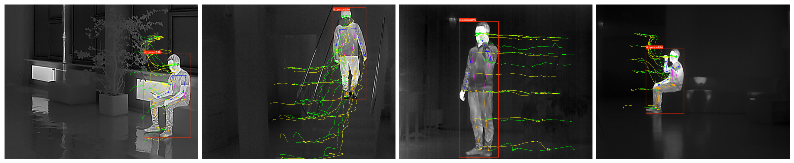
Figure 5 illustrates representative predicted keypoint trajectories over a 4 s temporal window obtained from the deployed pose-estimation pipeline. The trajectories demonstrate the temporal evolution of the detected body configuration and provide the spatial input subsequently used by the action-recognition models. The relative movement of individual keypoints across the observation window captures characteristic changes in body posture and motion, which are exploited by the temporal models for activity classification. The example also illustrates that the pose representation preserves temporal information while substantially reducing the input dimensionality compared with processing the original thermal images directly.

Figure 5. Predicted keypoints trajectories at 4 s temporal window.

4.2. Action Classification

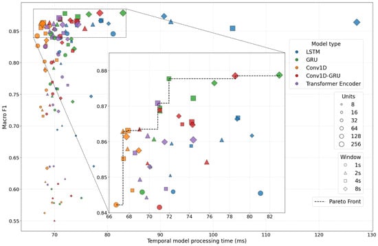
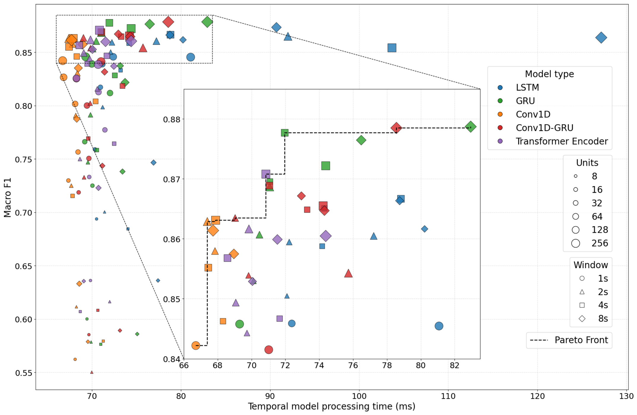
Figure 6 summarizes the relationship between action-recognition performance and computational cost for the evaluated temporal models. Each point represents one experimental configuration defined by the temporal architecture, network size, and observation window. The horizontal axis represents the temporal-model processing time on the Raspberry Pi 5 (excluding the selected YOLO-pose processing time), while the vertical axis represents the corresponding Macro F1-score. For each configuration, the reported value represents the mean obtained from five independent training/testing repetitions performed using five different random seeds. This repeated evaluation reduces the influence of stochastic training variability and provides a more representative estimate of the expected recognition performance and processing cost of each configuration. All recognition results were obtained on recordings of a single participant; they therefore characterize within-subject performance and do not measure generalization to unseen individuals (Section 5.2).

Figure 6. Macro F1-score versus temporal-model processing time on the Raspberry Pi 5 (mean of five seeds); the dashed line marks the Pareto front.

The results reveal a clear accuracy–latency trade-off among the evaluated temporal architectures, driven primarily by network size rather than by the length of the observation window. Averaged across all architectures and temporal windows, increasing the number of units N from 8 to 256 raises the mean Macro F1-score from approximately 0.61 to 0.86, while increasing the mean temporal-model processing time by only about 7 ms (from approximately 71 ms to 78 ms). The temporal window has a smaller and markedly architecture-dependent effect on processing time. For the Conv1D model, temporal-model processing time remains nearly constant across window lengths—for example, 66.7–67.9 ms for $N=256$ across 1–8 s windows—because the global-average-pooling stage collapses the temporal dimension independently of sequence length, while the corresponding Macro F1-score improves from 0.842 at a 1 s window to approximately 0.863 at 4–8 s windows. In contrast, the recurrent architectures show a much stronger dependence of processing time on window length: for $N=256$, GRU processing time increases from 69.3 ms at 1 s to 82.9 ms at 8 s, and LSTM increases far more steeply, from 81.1 ms to 127.2 ms over the same range, without a corresponding advantage in recognition performance.

Convolutional and hybrid convolutional-recurrent architectures occupy the low-latency end of the accuracy–latency space: five of the eight Pareto-optimal configurations in Table 3 are Conv1D or Conv1D-GRU, reaching Macro F1-scores of 0.842–0.878 at total processing times of 154–166 ms. The GRU architecture achieves the highest mean Macro F1-score observed in this study ($0.879\pm 0.005$, $N=256$, 8 s window), but this is within seed variability of the 128-unit GRU ($0.878\pm 0.008$) and the Conv1D-GRU ($0.878\pm 0.009$), and at a higher processing cost (82.9 ms) than the Conv1D-GRU with the same size (78.6 ms). The LSTM architecture reaches comparable Macro F1-scores for large network sizes, but its consistently higher and more steeply growing processing time means that no LSTM configuration lies on the Pareto frontier. The Transformer encoder appears on the frontier only once ($N=256$, 4 s window, 0.871 at 70.8 ms) and is otherwise dominated by the Conv1D, Conv1D-GRU, and GRU models. These results indicate that convolutional and hybrid architectures provide the most favorable trade-off for real-time deployment on the Raspberry Pi 5, whereas the differences between the best configurations (0.871–0.879) are small.

Table 3. Pareto-optimal temporal action-recognition configurations on the Raspberry Pi 5. The derived FPS = 1000/total time; frames arriving during processing are skipped.

Model	Units	Temporal Window, s	Sequence Length	Temporal Model Time, ms	Total Time, ms	FPS	Macro F1
Conv1D	256	1	6	66.7 ± 1.4	153.8 ± 2.5	6.5	0.842 ± 0.016
Conv1D	256	2	13	67.4 ± 1.4	155.2 ± 3.4	6.4	0.863 ± 0.008
Conv1D	256	4	25	67.9 ± 1.7	155.8 ± 4.8	6.4	0.863 ± 0.015
Conv1D-GRU	128	2	13	69.0 ± 1.5	155.9 ± 2.0	6.4	0.864 ± 0.003
Transformer-encoder	256	4	25	70.8 ± 2.0	157.1 ± 2.8	6.4	0.871 ± 0.005
GRU	128	4	25	72.0 ± 1.8	158.1 ± 2.5	6.3	0.878 ± 0.008
Conv1D-GRU	256	8	50	78.6 ± 2.1	166.3 ± 3.9	6.0	0.878 ± 0.009
GRU	256	8	50	82.9 ± 2.4	171.1 ± 3.6	5.8	0.879 ± 0.005

The resulting Pareto-optimal configurations are summarized in Table 3 and marked by the dashed Pareto front in Figure 6, where the inset enlarges the region of the highest Macro F1-scores; marker size and shape encode the network size and the observation window (see the legend). Pareto optimality is evaluated with respect to the temporal-model processing time, since this isolates the computational cost attributable to the temporal architecture itself, independent of the shared YOLO-pose front end; the corresponding total processing time is reported alongside for reference. Temporal-model and total processing times in Table 3 are reported as mean ± standard deviation over the five independent training/testing repetitions. The resulting frontier contains configurations from the Conv1D, Conv1D-GRU, GRU, and Transformer-encoder architectures. At the low-latency end of the frontier, the Conv1D model with 256 units and a 1 s temporal window achieves a Macro F1-score of 0.842 at a temporal-model processing time of approximately 67 ms (total processing time of approximately 154 ms). Increasing the model capacity and temporal window progressively improves recognition performance, with the highest Macro F1-score of 0.879 obtained by the 256-unit GRU using an 8 s window at a temporal-model processing time of approximately 83 ms (total processing time of approximately 171 ms). The intermediate configurations provide a range of accuracy–latency operating points, allowing the deployment configuration to be selected according to the required balance between recognition performance and real-time responsiveness.

Macro F1 is reported as mean ± standard deviation (sample SD, $n=5$ seeds); each seed changes both the assignment of recordings to the training, validation and test sets and the weight initialization. The SD of the Pareto-optimal configurations ranges from 0.003 to 0.016, which is larger than the difference among the four best configurations (0.871–0.879). These configurations therefore cannot be ranked reliably by Macro F1, and the Pareto frontier, computed from mean values, should be read as a set of comparable operating points that differ mainly in latency.

Table 4 presents a class-wise evaluation of one Pareto-optimal configuration, selected as an illustrative example rather than as the single recommended operating point. The example shown is the Conv1D-GRU architecture with 256 units, an 8 s temporal window, and a sequence length of 50 samples, corresponding to the configuration with a Macro F1-score of 0.878 in Table 3. Precision, recall, and F1-score are reported separately for each of the six activity classes (means over five seeds). The class-wise F1-scores lie in a narrow range of 0.857–0.895, with the highest value for standing (0.895) and the lowest for drinking (0.857) and walking (0.861). The lower score for drinking is consistent with it being the least represented activity in the dataset (Section 3.1), but the differences between classes are small. This configuration therefore provides balanced classification performance across the six activities while maintaining the computational efficiency required for edge deployment on the Raspberry Pi 5.

Table 4. Class-wise precision, recall, and F1-score for the selected Conv1D-GRU configuration with 256 units, an 8 s temporal window, and a sequence length of 50 samples.

Action	Precision	Recall	F1	Macro F1
Walking	0.849	0.874	0.861	0.878
Sitting	0.888	0.892	0.889
Standing	0.897	0.894	0.895
Lying	0.889	0.883	0.886
Calling	0.874	0.893	0.884
Drinking	0.854	0.861	0.857

The purpose of Table 4 is to illustrate the class-wise classification performance for one representative configuration, rather than to report precision, recall, and F1-score for every evaluated configuration. Since the complete experimental evaluation includes multiple architectures, network sizes, and temporal windows, presenting all class-wise metrics here would substantially increase the length of the manuscript without adding to the main accuracy–latency analysis in Table 3. The complete set of experimental results, together with the evaluation scripts and the annotated dataset, is made available through the associated repository (see the Data Availability Statement), allowing the reported results to be further inspected and reproduced.

4.3. End-to-End Throughput, Latency and Definition of Real-Time Operation

In this study, real-time operation is defined by three measurable conditions: (1) no backlog: surplus camera frames are skipped and never queued, so latency does not accumulate; (2) the sustained throughput of the complete RTSP-to-classification pipeline is within 10% of the sampling rate used for sequence construction (6.25 FPS, i.e., ≥5.6 FPS), so that the effective window length deviates from its nominal value by less than 10%; and (3) the processing latency of a frame is below 1 s. In addition, the response delay to an activity change is reported and compared with the time scale of the monitored activities (postures and daily actions that persist for seconds to minutes). All Pareto-optimal configurations satisfy (1)–(3).

Pose estimation and temporal classification are executed sequentially on the same CPU, so the cycle time of the pipeline equals the total processing time in Table 3 (154–171 ms), corresponding to 5.8–6.5 FPS. The camera delivers 25 FPS; therefore, frames are dropped by design: after each cycle the pipeline takes the most recent frame from the RTSP stream and discards the older ones, so that approximately three of every four frames are skipped and no queue forms. The recordings used for training and testing were decimated by the same factor of four (160 ms). In live operation the interval between processed frames is quantized to the 40 ms camera period; it is mostly four frames at 6.4 FPS and alternates between four and five frames for the 8 s configurations (6.0 and 5.8 FPS), whose effective window is therefore slightly longer than nominal (up to about 8.6 s). This timing jitter was not included in training.

Two quantities are distinguished. The processing latency of a frame is:

$$L_{\mathrm{proc}}=t_{\mathrm{RTSP}}+t_{\mathrm{pose}}+t_{\mathrm{temp}},$$

(2)

where $t_{\mathrm{RTSP}}$ is the delay introduced by the camera (encoding, wireless transmission, decoding and buffering), $t_{\mathrm{pose}}$ is the YOLO26n-pose/NCNN time per frame and $t_{\mathrm{temp}}$ is the temporal-model time; $t_{\mathrm{pose}}+t_{\mathrm{temp}}$ is the total time in Table 3. The response latency to a change of activity is:

$$L_{\mathrm{resp}}=L_{\mathrm{proc}}+\alpha W,\hspace{1em}0\le \alpha \le 1,$$

(3)

where W is the observation window. Because each sequence is labeled by its last frame, the window still contains mostly the previous activity right after a transition, and the output is expected to change once the new activity occupies about half of the window ($\alpha \approx 0.5$). The case $\alpha =1$ (the window fully filled by the new activity, as also required after start-up) is the upper bound. The value of $\alpha$ was not measured and is treated as an analytical estimate. $t_{\mathrm{RTSP}}$ was measured as approximately 0.5 s for the Lynx L15 stream.

Table 5 lists these values for the Pareto-optimal configurations. The processing latency is nearly constant (0.65–0.67 s) and dominated by the camera stream, whereas the response latency is dominated by the window: 1.15 s for the 1 s window and 4.67 s for the 8 s window at $\alpha =0.5$, and up to 1.65 s and 8.67 s at $\alpha =1$. The gain in Macro F1 from long windows is therefore paid for mainly in response time and not in computation. For example, the 8 s GRU (0.879) differs from the 4 s GRU with 128 units (0.878) by only 0.001, well below the seed SD (0.005–0.008), while adding about 2 s of nominal response latency, so the 4 s configuration is the more practical operating point. Configurations with 1–2 s windows respond within about 1.2–1.7 s with Macro F1 of 0.842–0.864. Such delays are acceptable for monitoring postures and daily activities, but 4–8 s windows are not suitable for applications needing sub-second reaction, such as fall alarms, which are outside the six classes studied here.

Table 5. End-to-end latency of the Pareto-optimal configurations on the Raspberry Pi 5 ($t_{\mathrm{RTSP}}=0.5$ s; $L_{\mathrm{resp}}$ for $\alpha =0.5$ and the upper bound $\alpha =1$).

Model	Units	W, s	Total Time, ms	FPS	${\mathit{L}}_{\mathbf{proc}}$, s	${\mathit{L}}_{\mathbf{resp}}$ ($\mathit{\alpha } = 0.5$), s	${\mathit{L}}_{\mathbf{resp}}$ ($\mathit{\alpha } = 1$), s
Conv1D	256	1	153.8	6.5	0.65	1.15	1.65
Conv1D	256	2	155.2	6.4	0.66	1.66	2.66
Conv1D	256	4	155.8	6.4	0.66	2.66	4.66
Conv1D-GRU	128	2	155.9	6.4	0.66	1.66	2.66
Transformer-encoder	256	4	157.1	6.4	0.66	2.66	4.66
GRU	128	4	158.1	6.3	0.66	2.66	4.66
Conv1D-GRU	256	8	166.3	6.0	0.67	4.67	8.67
GRU	256	8	171.1	5.8	0.67	4.67	8.67

To quantify the cost of skipping frames, the experiments were repeated at the original 25 FPS (sequence lengths of 25, 50, 100, and 200 samples, stride of five frames). Averaged over architectures, network sizes, and windows, the Macro F1-score was 0.795 at 25 FPS and 0.787 at approximately 6 FPS (mean difference 0.008; per-configuration differences, 25 FPS minus 6 FPS, ranged from −0.12 to +0.05). The best configuration reached 0.901 at 25 FPS (GRU, $N=256$, 4 s) versus 0.879 at 6 FPS, i.e., a loss of 0.022 at the best operating point, which is the price of real-time operation.

5. Discussion

5.1. Findings

The results show that a complete thermal pose estimation and temporal action recognition pipeline can operate in real-time entirely on the Raspberry Pi 5 CPU (Section 4.3: 5.8–6.5 FPS, processing latency 0.65–0.67 s), without any dedicated neural-network accelerator. Export format proved to be the single largest factor in achieving this: NCNN reduced YOLO-pose inference time by approximately 1.9–2.9× relative to native PyTorch and ONNX Runtime while also consuming the least power in every configuration (Table 2), making the nano-variant models the only YOLO-pose configuration compatible with real-time temporal sequence construction among those evaluated. Among the nano variants, YOLO26n-pose in NCNN format offered the best accuracy at equivalent cost (92.6% pose mAP50–95 at approximately 86 ms per frame, 0.5 percentage points below its native PyTorch accuracy), and was used as the pose front end for all subsequent experiments.

For the temporal action recognition stage, network size was found to be the dominant driver of recognition performance, raising the mean Macro F1-score from approximately 0.61 to 0.86 as N increased from 8 to 256 units, at a comparatively small average latency cost of roughly 7 ms. The length of the observation window had a smaller and strongly architecture-dependent effect: Conv1D’s processing time remained essentially flat across window lengths due to global average pooling, whereas the recurrent architectures, and LSTM in particular, scaled much more steeply with window length without a corresponding accuracy advantage. Consistent with this, the Conv1D and Conv1D-GRU architectures occupied the low-latency end of the accuracy–latency Pareto frontier (Figure 6, Table 3), with GRU reaching the single highest Macro F1-score observed (0.879) at higher latency, while LSTM never appeared on the Pareto frontier and the Transformer encoder only once.

5.2. Limitations

The thermal image and activity datasets were collected from a single male participant across eight indoor rooms at a consistent ambient temperature of approximately 21 °C. Consequently, the reported recognition scores, of up to 0.879, characterize within-subject performance. Although the test recordings were excluded from training (Section 3.4), they originate from the same person, camera, and activity protocol, so part of the score may reflect person-specific movement patterns rather than generalizable activity recognition. Varying clothing and rooms only partly mitigates this, because it does not introduce variation in age, gender, body size, body-heat distribution, or gait, all of which can alter the thermal silhouette and the keypoint trajectories used by the temporal models. Evidence from the pose-estimation stage points in the same direction: when the YOLO26s-pose model trained on this dataset was applied without fine-tuning to two public multi-subject thermal pose datasets, its pose mAP50–95 decreased from 0.942 to 0.617 and 0.544 [18], indicating that keypoint quality, and thus the input of the temporal classifiers, can degrade under subject and sensor shift. The results should therefore be interpreted as evidence of feasibility and of the relative behavior of architectures, export formats, and sampling rates under identical conditions, not as a population-level estimate of recognition accuracy. The six activity classes are also relatively coarse and do not include commonly targeted use cases such as falls, multi-person scenes, or occluded or non-frontal viewpoints, all of which are known from the reviewed literature to reduce the reliability of thermal keypoint extraction. Simultaneous labels in the dataset are limited to a posture or walking combined with calling or drinking, and no other combinations (e.g., two simultaneous postures or multiple persons) were annotated; the multi-label evaluation therefore does not cover more complex concurrent activities.

The evaluation concentrates on a single person whose body is fully visible. Real surveillance and assisted-living scenes frequently contain several people, body occlusions (e.g., by furniture) and lateral postures with hidden far-side limbs. Lateral and oblique orientations are present in the recordings, but the robustness of the pipeline to occlusion-induced keypoint loss or errors and to multi-person scenes (which additionally require tracking to keep one pose sequence per person) was not evaluated. The only robustness evidence available here is the variability across five random recording-level splits (Table 3), the sensitivity to the sampling rate (Section 4.3) and the degradation of pose accuracy under subject and sensor shift [17]. The system should therefore be regarded as a feasibility study and not as validated for safety-critical deployment.

The evaluation is further limited to a single edge platform, the Raspberry Pi 5, and a single thermal sensor, the Lynx L15 monocular; results may not transfer directly to other CPU-only boards, other thermal cameras with different resolutions or noise characteristics, or platforms equipped with a neural accelerator. In addition, while the pose estimation stage was evaluated across three export formats and benefited substantially from NCNN conversion, the temporal action recognition models were evaluated only in their native TensorFlow/Keras form; conversion to a lighter-weight runtime or the application of quantization, both of which are common in comparable Raspberry Pi deployments (Table 1), was not explored and could plausibly narrow the latency gap between the recurrent and convolutional architectures observed in Section 4.2. Moreover, the temporal models were trained on strictly decimated sequences, whereas live frame intervals vary slightly (Section 4.3); the effect of this jitter, for example through random frame-step augmentation, was not evaluated.

6. Conclusions and Outlooks

This study developed and evaluated a complete thermal pose-based activity recognition pipeline, integrating RTSP video acquisition, YOLO-pose estimation, and lightweight temporal classification on a CPU-only Raspberry Pi 5. Using a purpose-built thermal dataset of 93,070 annotated frames across six activity classes, the evaluation jointly characterized pose-estimation accuracy, export-format efficiency, and temporal-architecture trade-offs under a common protocol with recording-level train/validation/test splits.

The results show that export format, rather than model family alone, is decisive for real-time feasibility on accelerator-free hardware: NCNN reduced YOLO-pose inference time by up to 2.9× relative to native PyTorch while also drawing the least power, making YOLO26n-pose in NCNN format (92.6% mAP50–95 at approximately 86 ms per frame) the pose-estimation configuration used throughout. For temporal classification, network size was the dominant factor in recognition performance. Conv1D and Conv1D-GRU occupied the low-latency end of the accuracy–latency trade-off, GRU reached the highest Macro F1-score of 0.879, the Transformer encoder appeared on the Pareto frontier only once, and LSTM did not reach it. All scores were obtained on held-out recordings of a single participant.

These findings indicate that real-time thermal activity recognition with a Macro F1-score of up to 0.88 is feasible entirely on CPU-only edge hardware, within the single-participant setting evaluated here, through the combined selection of an efficient export format and an appropriately sized temporal model, without requiring a dedicated neural-network accelerator. Future work should first extend this evaluation to multiple participants spanning different ages, genders, body sizes, and gait patterns, and then to additional thermal sensors, edge platforms, and quantized or converted temporal-model runtimes, to assess the generalizability of the proposed pipeline, and to occlusion-rich, lateral-view and multi-person recordings with tracking, to assess robustness for assisted living and safety monitoring.

References

- Najeh, H.; Lohr, C.; Leduc, B. Real-time human activity recognition on embedded equipment: A comparative study. Appl. Sci. 2024, 14, 2377. [Google Scholar] [CrossRef] [Scilit]
- Cao, B.; Zhao, L.; Zhao, H.; Xi, H.; Xu, L.; Yang, S. A Lightweight and Efficient Deep Learning Model Based on Improved YOLOv12 for Fall Detection in College Sport Activities. Information 2026, 17, 684. [Google Scholar] [CrossRef] [Scilit]
- Liang, Y.; Kang, H.; Zhong, H. RMDD: Raspberry Pi-Based Multimodal Dangerous Driving Behavior Detection. Electronics 2026, 15, 3828. [Google Scholar] [CrossRef] [Scilit]
- Zhou, H.; Zhang, X.; Feng, Y.; Zhang, T.; Xiong, L. Efficient human activity recognition on edge devices using DeepConv LSTM architectures. Sci. Rep. 2025, 15, 13830. [Google Scholar] [CrossRef] [Scilit] [PubMed]
- Chen, I.C.; Wang, C.J.; Wen, C.K.; Tzou, S.J. Multi-person pose estimation using thermal images. IEEE Access 2020, 8, 174964–174971. [Google Scholar] [CrossRef] [Scilit]
- Zang, Y.; Fan, C.; Zheng, Z.; Yang, D. Pose estimation at night in infrared images using a lightweight multi-stage attention network. Signal Image Video Process. 2021, 15, 1757–1765. [Google Scholar] [CrossRef] [Scilit]
- Cormier, M.; Yi, C.N.Z.; Specker, A.; Blaß, B.; Heizmann, M.; Beyerer, J. Leveraging Thermal Imaging for Robust Human Pose Estimation in Low-Light Vision. In Asian Conference on Computer Vision; Springer: Singapore, 2024; pp. 67–83. [Google Scholar]
- Manda, A.; Pardhasaradhi, B.; Cenkeramaddi, L.R. TMCR Edge-YOLO: Thermal Sensing-based Mobility-Context Recognition on the Edge. IEEE Sens. J. 2026. [Google Scholar] [CrossRef] [Scilit]
- Cormier, M.; Specker, A.; Beyerer, J. UPPET: Unified Pedestrian Pose Estimation in Thermal Imaging. In 2025 IEEE/CVF Conference on Computer Vision and Pattern Recognition Workshops (CVPRW); IEEE: New York, NY, USA, 2025; pp. 4551–4560. [Google Scholar]
- Zeng, L.; Huang, C.; Xie, R.; Huang, Z.; Guo, Y.; He, L.; Xie, Z.; Xing, G. ThermiKit: Edge-Optimized LWIR Analytics with Agent-Driven Interactions. In Proceedings of the 2025 ACM International Workshop on Thermal Sensing and Computing; Association for Computing Machinery: New York, NY, USA, 2025; pp. 40–46. [Google Scholar]
- Lupión, M.; González-Ruiz, V.; Medina-Quero, J.; Sanjuan, J.F.; Ortigosa, P.M. THPoseLite, a lightweight neural network for detecting pose in thermal images. IEEE Internet Things J. 2023, 10, 15060–15073. [Google Scholar] [CrossRef] [Scilit]
- Smith, J.; Loncomilla, P.; Ruiz-Del-Solar, J. Human pose estimation using thermal images. IEEE Access 2023, 11, 35352–35370. [Google Scholar] [CrossRef] [Scilit]
- Kuzdeuov, A.; Zakaryanov, M.; Tleuliyev, A.; Varol, H.A. OpenThermalPose2: Extending the Open-Source Annotated Thermal Human Pose Dataset with More Data, Subjects, and Poses. IEEE Trans. Biom. Behav. Identity Sci. 2025, 7, 902–913. [Google Scholar] [CrossRef] [Scilit]
- Bharathi, A.; Sanku, R.; Sridevi, M.; Manusubramanian, S.; Chandar, S.K. Real-time human action prediction using pose estimation with attention-based LSTM network. Signal Image Video Process. 2024, 18, 3255–3264. [Google Scholar] [CrossRef] [Scilit]
- Wang, Z.; Sun, H.; Calautit, J.K.; Yang, M.; Chen, J.; Guan, R.; Darkwa, J. A novel lightweight skeletal temporal model for real-time, computationally efficient recognition of occupant thermal adaptation behavior. In Building Simulation; Springer: Berlin/Heidelberg, Germany, 2025; Volume 18, pp. 2849–2874. [Google Scholar]
- Sykes, E.R. Next-generation fall detection: Harnessing human pose estimation and transformer technology. Health Syst. 2025, 14, 85–103. [Google Scholar] [CrossRef] [Scilit] [PubMed]
- Vdoviak, G.; Sledevič, T.; Abromavičius, V.; Navakauskas, D.; Kaklauskas, A. Efficient Thermal Pose Estimation: Balancing Accuracy and Edge Deployment for Smart Home Activity Recognition. Sensors 2026, 26, 1774. [Google Scholar] [CrossRef] [Scilit] [PubMed]
- Vdoviak, G.; Sledevič, T.; Matuzevičius, D. Accelerator-Free Thermal Pose Estimation: Accuracy–Efficiency Trade-Offs on the Raspberry Pi 5. Sensors 2026, 26, 5188. [Google Scholar] [CrossRef] [Scilit] [PubMed]
- Vijay, H.; Mathur, S.; Agarwal, S.; Perumal, T.; Sharma, A. MotionScope AI: Comprehensive Human Activity Recognition Through Integrated Pose Analysis and Temporal Modeling. IEEE Sens. J. 2026, 7, 10872–10882. [Google Scholar] [CrossRef] [Scilit]
- Luo, Q.; Zhou, H.; Wu, M.; Zhou, Q. Low-Light Pose-Action Collaborative Network for Industrial Monitoring in Power Systems. Electronics 2026, 15, 199. [Google Scholar] [CrossRef] [Scilit]
- Wanna, Y.; Wiratchawa, K.; Intharah, T. TinyAct: A framework for real-time action recognition in the cloud through distillation learning. PLoS ONE 2026, 21, e0347245. [Google Scholar] [CrossRef] [Scilit] [PubMed]
- Park, J.; Yang, K.O.; Park, S.; Choi, J.W. Human Daily Indoor Action (HDIA) Dataset: Privacy-Preserving Human Action Recognition Using Infrared Camera and Wearable Armband Sensors. IEEE Access 2025, 13, 60822–60832. [Google Scholar] [CrossRef] [Scilit]
- Guo, Y.; Chen, Y.; Deng, J.; Li, S.; Zhou, H. Identity-preserved human posture detection in infrared thermal images: A benchmark. Sensors 2022, 23, 92. [Google Scholar] [CrossRef] [Scilit] [PubMed]
- Nabizade, M.; Yahiaoui, R.; Lajoie, I.; Nacer, N.; Auber, F.; Fayad, M. Real-Time Vision-Based Fall Detection Systems for the Elderly: A Systematic Review. Sensors 2026, 26, 5069. [Google Scholar] [CrossRef] [Scilit] [PubMed]
- Cho, W.; Bang, S.O.; Choi, H.S.; Kwon, K.T.; Shin, S.W.; Roh, J.S.; Lim, J.M.; Park, H.M. A Lightweight CNN–TCN–Attention Framework for Low-Latency Pre-Fall Transition and Fall Recognition on Resource-Constrained Edge Devices. Electronics 2026, 15, 3748. [Google Scholar] [CrossRef] [Scilit]
- Huang, W.; Wu, M.; Chen, W.; Zhou, Q. A Bio-Inspired Lightweight Human Action Recognition Method Based on Human Keypoint Detection. Biomimetics 2026, 11, 355. [Google Scholar] [CrossRef] [Scilit] [PubMed]
- Le, H.; Lu, C.K.; Wang, W.Y.; Hsu, C.C. Skeleton-Based Human Action Recognition Using Multi-Type Input Data on Edge Devices in Internet of Things Systems. IEEE Internet Things J. 2026, 13, 17319–17335. [Google Scholar] [CrossRef] [Scilit]
- Le, H.; Lu, C.K.; Hsu, C.C. TS-ResCNN: Efficient Skeleton-Based Action Recognition for Edge IoT Sensor Systems. IEEE Sens. J. 2026, 26, 12613–12622. [Google Scholar] [CrossRef] [Scilit]
- Sharma, V.; Sharma, A.; Saini, S. Real-time attention-based embedded LSTM for dynamic sign language recognition on edge devices. J. Real-Time Image Process. 2024, 21, 53. [Google Scholar] [CrossRef] [Scilit]
- Bach, N.C.; Van Chi, N.; Cuong, D.D.; Tuan, N.A.; Kieu, T.Q.T.; Phuong, N.T.; Thien, N.D.; Thao, L.Q. A lightweight and efficient deep learning model for real-time fall detection on edge device. Biomed. Signal Process. Control 2026, 113, 108942. [Google Scholar] [CrossRef] [Scilit]
- Wang, Y.; Wu, Y.; Ogai, H.; Dong, Y.; Tateno, S. Edge-Oriented Person Activity Recognition and Alert System for Ensuring Safety of Independent Elderly at Home. In 2025 8th International Conference on Information Communication and Signal Processing (ICICSP); IEEE: New York, NY, USA, 2025; pp. 551–555. [Google Scholar]
- Analia, R.; Forster, A.; Xie, S.Q.; Zhang, Z. Privacy-Preserving Approach for Early Detection of Long-Lie Incidents: A Pilot Study with Healthy Subjects. Sensors 2025, 25, 3836. [Google Scholar] [CrossRef] [Scilit] [PubMed]
Disclaimer/Publisher’s Note: The statements, opinions and data contained in all publications are solely those of the individual author(s) and contributor(s) and not of MDPI and/or the editor(s). MDPI and/or the editor(s) disclaim responsibility for any injury to people or property resulting from any ideas, methods, instructions or products referred to in the content. |
© 2026 by the authors. Licensee MDPI, Basel, Switzerland. This article is an open access article distributed under the terms and conditions of the Creative Commons Attribution (CC BY) license.