FEM-PDNet: Evaluating Fixed and Learned Logit Fusion for Pre-Drowsiness Classification on UTA-RLDD

Abstract

This study evaluates fixed and learned logit fusion for clip-level pre-drowsiness classification on an adaptively curated cohort from the University of Texas at Arlington Real-Life Drowsiness Dataset (UTA-RLDD). The target is an operationally defined visual state, not an independently established physiological condition or a prospective early-warning event. FaceMesh-Enhanced Multi-cue Pre-Drowsiness Network (FEM-PDNet) combines RGB temporal logits with behavior–motion logits derived from FaceMesh, optical flow, and frame differences. A blinded second review yielded 206 agreement-confirmed clips from 51 subjects. Sixteen configurations shared subject-disjoint five-fold partitions, five seeds, validation-selected checkpoints, and a fixed 0.5 threshold. FEM-PDNet obtained macro-F1 $0.719\pm 0.143$ and pre-drowsy recall $0.578\pm 0.282$. Its difference from the tested concatenation implementation was 0.2344 (Holm-adjusted $p=0.0260$ across 16 contrasts), but fixed-weight controls did not establish an independent benefit of coefficient learning. The behavior–motion multilayer perceptron (MLP) obtained higher mean macro-F1 ($0.823\pm 0.017$) than FEM-PDNet. Initialization and joint-feature-training analyses further characterized fusion sensitivity. Post-hoc branch diagnostics counted 15 corrected and 99 introduced errors relative to the feature branch across 1030 correlated clip–seed evaluations. These findings are conditional retrospective comparisons on a previously inspected cohort, not independent confirmation of generalization or the superiority of learned fusion.

1. Introduction

According to a press release from the Korea Road Traffic Authority, 5688 drowsy-driving traffic accidents occurred between 2021 and 2023, corresponding to approximately 5.2 cases per day. The fatality rate of drowsy-driving accidents was 2.7 deaths per 100 crashes, nearly twice the overall traffic-accident fatality rate of 1.4 deaths per 100 crashes [1]. These statistics indicate the need to detect signs of drowsiness before they develop into an overtly drowsy state.

Drowsiness-detection methods use physiological signals, driving patterns, or vision [2,3]. Physiological and subjective measures assess sleepiness and fatigue but may require intrusive or contact sensors [4,5,6,7]. Vehicle-motion indicators provide noncontact alternatives but vary with road conditions and driving habits [2,3,8]. Vision-based methods instead estimate eye closure, blinking, yawning, head pose, and gaze from camera data [9,10,11,12].

Early vision methods used eye closure, mouth opening, and facial orientation [10,11,13,14]; YawDD and DROZY supported evaluation of yawning and multimodal cues [15,16]. Recent methods use CNNs, three-dimensional CNNs, LSTMs, landmark toolkits, and mobile implementations to learn appearance and motion patterns [17,18,19,20,21,22,23]. Most formulate alert-versus-drowsy or multilevel classification, whereas the brief, normal-like cues of the intermediate pre-drowsy state remain difficult to detect [3,17,18,19,20,24].

Recent approaches address different aspects of driver-state modeling. FastKAN-DDD uses radial-basis-function networks and post-training quantization for lightweight drowsiness classification [25], whereas DFD-CLIP extends CLIP with temporal modeling and adaptive prompts linked to facial-behavior descriptions [26]. Appearance–motion integration also follows the broader two-stream approach to video recognition [22]. In contrast, the present study examines representation concatenation and late logit fusion of RGB appearance with explicit behavior–motion variables extracted from the same videos. These are related visual representations, not independent sensing modalities. The contribution is a controlled comparison of fusion with fixed weighting and component models, including cases in which adding a branch reduces performance; published results on different labels and partitions are not treated as directly comparable.

This study uses FEM-PDNet to examine RGB and behavior–motion logit fusion under matched subject partitions. Three questions guide the interpretation: whether learning scalar coefficients adds value beyond fixed weighting; whether the fused model improves on its component models; and how initialization and feature-branch optimization affect the results. The comparison includes fixed equal and fixed unequal weights, independently evaluated branches, feature concatenation, alternative initializations, and joint-feature training.

The contribution is an empirical evaluation of these distinctions, supported by fold/seed results, weighted-margin diagnostics, and processing-cost measurements. Corrections and introduced errors are reported relative to the feature branch within the trained fusion model, separately from comparisons with independently trained models. These analyses characterize the evaluated implementations on adaptively curated UTA-RLDD clips; they do not assume that the two branches are complementary or that coefficient learning is intrinsically beneficial. Negative and mixed outcomes are part of the main empirical result. Recent reference-based baselines and label-scope, non-overlap, and prevalence analyses delimit the scope of the findings.

2. Study Design and Model Configurations

This section describes clip construction, annotation, and the model configurations used to compare fixed and learned fusion. FEM-PDNet denotes the reference learned-weight configuration; its component and fixed-weight controls test which aspects of the combined model contribute to the observed results.

2.1. Dataset

This study used the University of Texas at Arlington Real-Life Drowsiness Dataset (UTA-RLDD) RGB video dataset [24], which contains approximately 30 h of recordings from 60 subjects. The recordings were acquired with mobile phones or webcams in indoor real-life environments rather than during actual driving. Its original labels represent alert, low-vigilance, and drowsy states at the video level. Because a video-level label does not describe every short interval, the original labels were not used directly as clip-level ground truth.

Inspection of the videos showed that alert behavior, subtle drowsiness-related cues, and overt drowsiness could occur within the same source recording. The task was defined as classification of the behavioral state observed in the current clip. The pre-drowsy label denotes operationally defined subtle cues without overt drowsiness; it does not establish prediction of a subsequent drowsiness event or a lead-time horizon.

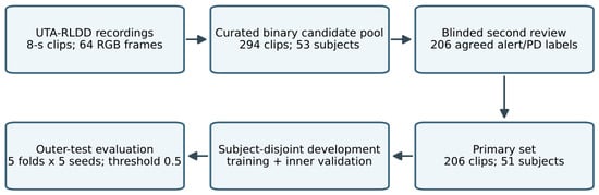
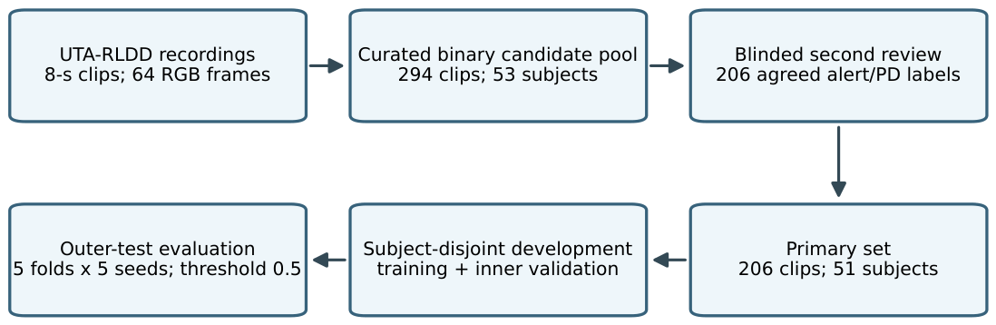
Candidate clips were generated using 8 s windows and sampled at 8 frames per second, giving 64 RGB frames per clip. Figure 1 summarizes the overall workflow for clip generation, independent annotation, agreement-confirmed primary-set construction, and subject-wise outer-fold evaluation.

Figure 1. Workflow for curated clip selection, blinded second review, and the revised five-fold, five-seed primary evaluation.

The retained clip-generation implementation specifies a 2 s temporal stride. All 294 recorded candidate intervals are 8 s long, with start times on a 2 s grid. The retained intervals do not form an exhaustive sliding-window sequence because clips were accumulated through selection and re-review rounds.

Both annotators had backgrounds in artificial intelligence. Annotator A was the first author and had no prior experience in drowsiness annotation. Annotator B was not a coauthor and had previous experience with object detection of surface scratches on plastic products. Annotator B received the complete behavioral criteria before labeling, without access to model predictions or probabilities. The annotators did not jointly review a written rubric or conduct a practice/calibration session before labeling. Clips were presented without the original dataset labels; the second annotator also had no access to the initial clip-level decisions.

Retained contemporaneous guidance for later candidate-review rounds distinguishes normal blinking, subtle drowsiness-related cues, overt drowsiness, and ambiguous or unreadable clips. The surviving protocol document retrospectively describes labels already assigned; the records do not establish a single versioned rubric fixed before all rounds. B received behavioral criteria, but the retained records do not establish a standardized training or calibration procedure.

Candidate clips first received an alert or pre-drowsy label from one annotator. A second annotator independently reviewed each clip without access to the initial decision and assigned alert, pre-drowsy, drowsy, or exclude. Alert required stable eye opening, gaze, facial orientation, and head movement. Pre-drowsy indicated slow blinking, eyelid drooping, yawning, gaze decline, or head lowering without overt drowsiness. Prolonged eye closure, marked head dropping, or another clear sign of overt drowsiness was labeled drowsy; clips that could not be judged reliably were excluded.

The accumulated reviewed pool contained 1858 clips from successive shortlisting and candidate-review rounds, rather than a single prespecified random sample. Its final recorded labels were 1284 alert, 147 pre-drowsy, 175 drowsy, and 252 exclude. The pool contained 596 clips from low-vigilance source recordings and 1262 from drowsy recordings. No originally alert recordings were represented, including in the earliest retained 345-clip shortlist. Later candidate-mining records show source-targeted expansion, but the initial reason for the absence of alert-source recordings is not established by the retained records. Supplementary Revision Table S12 summarizes these snapshots and evidence limits. The balanced binary pool retained all 147 pre-drowsy clips and 147 alert clips selected through multi-round readability review. Temporal overlap was not a strict exclusion criterion, and selection did not use a single prespecified random-sampling step. Thus, the 294 clips form a curated class-balanced candidate set rather than the natural label distribution. They covered 53 of 60 subjects.

Earlier test/error-review records contain five current candidate clips, including three primary clips; two primary clips changed from pre-drowsy to alert between retained pool snapshots. The records document error-informed selection of re-review targets and incorporation of review decisions into the pool. The annotator confirms that per-clip predicted labels and probabilities were not viewed during relabeling, but target selection was not independent of earlier outcomes. The cohort is therefore adaptively curated. This revision does not relabel or remove these clips; implications for inference are discussed in Section 4.

The annotators agreed on alert or pre-drowsy for 206 of 294 clips (70.1%). Among the 259 clips that the second annotator also classified as binary, agreement was 79.5% (206/259), with Cohen’s $\kappa =0.589$. These 206 cases (116 alert and 90 pre-drowsy) form the primary set.

For the 88 initial disagreements, the second annotator completed two additional blinded passes, with the clip order reshuffled for each pass. The final label was the majority of this annotator’s three decisions; the first annotator’s label did not enter this vote. If all three decisions differed, the clip was excluded. Of the 88 clips, 35 had unanimous review decisions, 48 had a two-of-three majority, and five had three different decisions. The resulting labels were 38 alert, 12 pre-drowsy, nine drowsy, and 29 exclude. Thus, 50 clips were added to the reviewed set, giving 256 clips (154 alert and 102 pre-drowsy). All three review sessions occurred on the same day, without a long washout interval, so repeat assessments may be affected by recall. These passes are repeated judgments by one annotator, not assessments by three independent annotators. Supplementary Revision Table S8 provides examples of the recorded decision paths.

The reviewed-set sensitivity additionally includes the 50 majority-assigned cases. All clips from a subject, including temporal overlaps, remained in one partition within each outer-fold evaluation; therefore, no overlapping pair crossed training, inner-validation, or outer-test partitions. Agreement filtering removed all clips for two subjects. Table 1 summarizes the sets.

Table 1. Label sets for primary and sensitivity analyses.

Set	Alert	Pre-Drowsy	Total	Subjects
Candidate	147	147	294	53
Primary	116	90	206	51
Reviewed	154	102	256	53

The source-label audit (Table 2) shows that the primary clips came from low-vigilance and drowsy recordings, with none from the originally alert recordings. In particular, 81 of 116 clip-level alert cases came from drowsy source videos. The original labels describe a predominant video-level state [24], whereas the assigned labels describe the selected interval. The shared visual cues in annotation and feature extraction, and the cohort’s source composition, are considered together in Section 4.

Table 2. Original source-video state versus assigned clip label.

Source State (File Code)	Candidate Alert	Candidate PD	Primary Alert	Primary PD
Alert (0)	0	0	0	0
Low vigilance (5)	55	18	35	7
Drowsy (10)	92	129	81	83

Candidate $n=294$; primary $n=206$. Original file codes 0/5/10 denote alert/low vigilance/drowsy. The intermediate state is stored as source code 1 with the alias pre_drowsy in the local metadata; this alias is not a clip-level diagnosis.

2.2. Evaluation and Ablation Strategy

The revised primary comparison uses the 206 agreement-confirmed clips, five subject-wise outer folds, and five training seeds. All configurations, including the behavior–motion-only MLP, are included. Each development fold is divided into subject-disjoint training and inner-validation sets. Training-only preprocessing and weighting, validation-only checkpoint selection, and the fixed 0.5 outer-test threshold are shared. The 256-clip reviewed-set and 192-clip non-overlap results retain their historical three-seed scope and are reported separately.

2.2.1. RGB-Only Baseline

The RGB-only baseline receives 64 RGB frames from each 8 s clip. A pretrained ResNet-18 [27] extracts frame features, a gated recurrent unit (GRU) [28] models their temporal order, and attention pooling produces RGB video logits. This tests RGB appearance and temporal context without engineered behavior or motion features.

Let $X^{\mathrm{rgb}}$ denote an input RGB clip consisting of $T=64$ temporally ordered frames. The tth frame satisfies $x_t\in {\mathbb{R}}^{H\times W\times 3}$, where H and W denote the frame height and width, respectively. The CNN extractor $f_{\mathrm{CNN}}(·)$ maps each frame to $r_t$, and a GRU processes the frame-feature sequence to obtain hidden states $h_t$. Attention pooling assigns the temporal weight ${\alpha }_t$ to each hidden state and produces the clip-level representation $z^{\mathrm{rgb}}$, which is mapped to the RGB logits ${\mathcal{l}}^{\mathrm{video}}$ and then converted into class probabilities through the softmax function. Here $g_{\mathrm{video}}$ is the 512–512–2 classification MLP specified below, rather than a single linear projection. The complete formulation is given in (1)–(8).

$$X^{\mathrm{rgb}}=(x_1,\dots ,x_T),T=64$$

(1)

$$x_t\in {\mathbb{R}}^{H\times W\times 3}$$

(2)

$$r_t=f_{\mathrm{CNN}}\left(x_t\right),t=1,\dots ,T$$

(3)

$$H^{\mathrm{rgb}}=\mathrm{GRU}(r_1,\dots ,r_T)=(h_1,\dots ,h_T)$$

(4)

$${\alpha }_t={\mathrm{softmax}}_t\left(w_a^{\top }{h}_t\right)$$

(5)

$$z^{\mathrm{rgb}}={\displaystyle \sum _{t=1}^T}{\alpha }_t{h}_t$$

(6)

$${\mathcal{l}}^{\mathrm{video}}=g_{\mathrm{video}}\left(z^{\mathrm{rgb}}\right)$$

(7)

$$p^{\mathrm{rgb}}=\mathrm{softmax}\left({\mathcal{l}}^{\mathrm{video}}\right)$$

(8)

2.2.2. Behavior and Motion Features

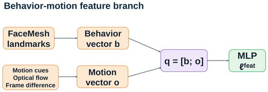
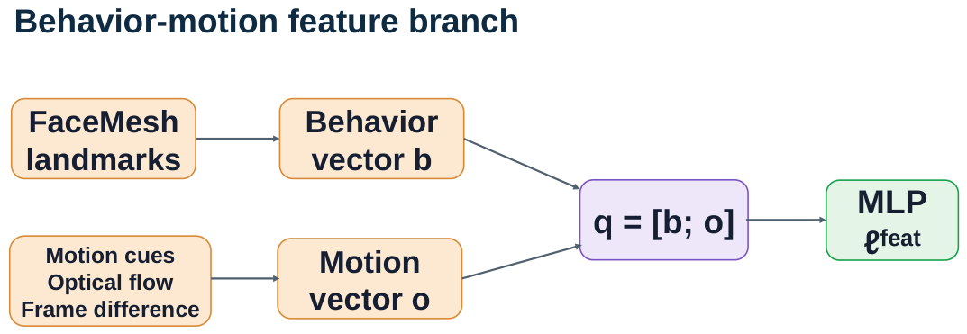
FaceMesh measurements [29,30] and motion statistics derived from optical flow and frame differences are summarized over each clip. The 30 FaceMesh-derived variables describe eye closure, blinking, mouth opening and yawning, gaze decline, head lowering, microevents, and temporal trends. The 11 motion variables comprise nine optical-flow statistics and two frame-difference statistics. A compact multilayer perceptron (MLP) maps the 41 variables to behavior–motion logits, as summarized in Figure 2.

Figure 2. Behavior–motion feature branch.

The behavior–motion-only MLP is included in the main results to test whether the RGB branch adds predictive value beyond these features.

Let $T_f\le 32$ and $T_m\le 16$ denote the numbers of uniformly sampled FaceMesh and grayscale motion frames. For consecutive grayscale frames $g_t$ and $g_{t+1}$ for $t=1,\dots ,T_m-1$, O denotes Farnebäck flow [31] implemented in OpenCV [32], and D denotes mean absolute grayscale difference; the underlying flow formulations are described in [31,33].

$$L_{1:T_f}=(L_1,\dots ,L_{T_f})$$

(9)

$$b=\psi \left(L_{1:T_f}\right)$$

(10)

$$\begin{array}{cc}\hfill F_t& =O(g_t,g_{t+1}),d_t=D(g_t,g_{t+1}),\hfill \\ \hfill & t=1,\dots ,T_m-1\hfill \end{array}$$

(11)

$$\begin{array}{cc}\hfill o& =\rho (F_{1:T_m-1},d_{1:T_m-1})\hfill \\ \hfill & =[o_{1:9}^{\mathrm{flow}};o_{1:2}^{\mathrm{diff}}]\in {\mathbb{R}}^{11}\hfill \end{array}$$

(12)

$$q=[b;o]$$

(13)

$${\mathcal{l}}^{\mathrm{feat}}=g_{\mathrm{feat}}\left(q\right)$$

(14)

$$p^{\mathrm{feat}}=\mathrm{softmax}\left({\mathcal{l}}^{\mathrm{feat}}\right)$$

(15)

$$L^{\mathrm{feat}}={\mathrm{CE}}_w(y,p^{\mathrm{feat}})$$

(16)

2.2.3. FEM-PDNet Learned-Weight Configuration

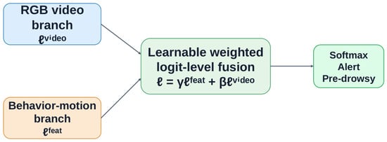
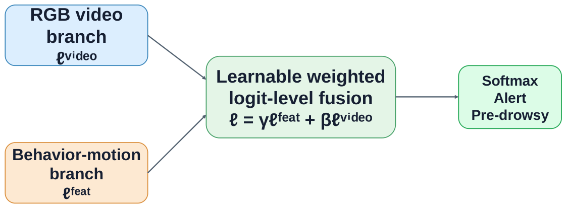
FEM-PDNet combines RGB video logits with behavior–motion logits from a feature MLP. Two learned scalar coefficients weight these vectors before the final softmax. This defines the evaluated model; whether learning the coefficients or adding the RGB branch improves classification is tested separately using the controls below. Figure 3 shows the architecture.

Figure 3. FEM-PDNet learned-weight configuration evaluated with fixed-weight and component controls.

Equations (1)–(7) define the RGB branch, and (9)–(14) define the behavior–motion branch. The resulting video and feature logits are combined as

$$\mathcal{l}=\gamma {\mathcal{l}}^{\mathrm{feat}}+\beta {\mathcal{l}}^{\mathrm{video}}$$

(17)

$$p=\mathrm{softmax}\left(\mathcal{l}\right)$$

(18)

$$L_{\mathrm{main}}={\mathrm{CE}}_w(y,p)$$

(19)

where $\gamma$ and $\beta$ are unconstrained learned scalars initialized to 0.70 and 0.05, respectively, and optimized jointly with the trainable RGB parameters using AdamW. They are not normalized to sum to one. Within each fold, the alert class weight was 1 and the pre-drowsy weight was the training-set alert-to-pre-drowsy ratio. The video/fusion loss ${\mathrm{CE}}_w$ used label smoothing of 0.05.

2.2.4. Model Summary

The visual branch used a frozen ImageNet-1K-pretrained ResNet-18 [27], a one-layer bidirectional GRU [28] with 256 units per direction, scalar attention, and a 512–512–2 rectified linear unit (ReLU) MLP with 0.35 dropout. The behavior–motion MLP used dimensions 41–64–32–2, batch normalization after the first layer, ReLU, and 0.35 dropout. The behavior–motion MLP checkpoint was selected using the inner-validation split and then frozen during fusion-model training. Its 41-dimensional input contained 30 FaceMesh-derived variables and 11 motion variables (nine optical-flow and two frame-difference statistics); definitions and fold-specific preprocessing are provided in Supplementary Revision Table S7. Table 3 summarizes the model components.

Table 3. Summary of FEM-PDNet components.

Component	Description
RGB branch	64 RGB frames; ResNet-18; GRU; attention pooling
Behavior cues	Eye-closure proportion; blink; mouth aspect ratio; yawning; gaze decline; head lowering
Motion cues	Optical-flow and frame-difference statistics
Feature branch	Behavior and motion vectors are mapped to behavior–motion logits
Fusion	Learnable weighted logit-level fusion

The executed internal RGB loader uniformly selected 64 indices from the existing JPEG frame cache, converted frames to RGB, resized them to $224\times 224$, converted them to tensors, and normalized channels using ImageNet means $(0.485,0.456,0.406)$ and standard deviations $(0.229,0.224,0.225)$. Training-only transforms were independently sampled per frame: color jitter with brightness/contrast/saturation ranges $0.18/0.18/0.10$ and no hue shift; $3\times 3$ Gaussian blur with standard deviation in $[0.1,1.0]$ and probability 0.12; grayscale, autocontrast, and sharpness adjustment (factor 1.5) with probabilities $0.05$, $0.10$, and $0.10$; and additive Gaussian tensor noise with standard deviation 0.015 and probability 0.15, clamped to $[0,1]$ before normalization. Validation and test used only resize, tensor conversion, and normalization. No stochastic crop or flip was applied by this loader. The retained records identify source intervals and cached frames but do not certify the complete historical cache-generation command or byte-identical source decoding.

2.3. Component-Wise Ablation Design

Architecture comparisons, coefficient-learning controls, and branch diagnostics address different questions. The concatenation contrast compares the tested integration implementations. Fixed-weight controls assess the incremental value of coefficient optimization. Standalone branches and within-model decision changes assess different aspects of branch value; a gain over concatenation alone does not establish either coefficient-learning benefit or complementarity. Behavior–motion only uses the independently selected 41-input MLP without RGB. RGB + FaceMesh uses the same weighted-logit architecture as FEM-PDNet but a 30-input FaceMesh MLP without the 11 motion variables. Full feature concatenation joins the 512-dimensional pooled RGB representation and the frozen MLP’s 32-dimensional hidden representation; a 544–512–2 ReLU head with 0.35 dropout predicts the classes. Thus, concatenation operates on learned representations, not directly on the 41 raw variables.

Fixed equal fusion keeps $(\gamma ,\beta )=(1,1)$ throughout training and evaluation. Fixed unequal fusion keeps $(0.70,0.05)$, matching the initialization of FEM-PDNet without coefficient learning. The equal and unequal controls differ in both branch ratio (1 versus 14) and total coefficient scale (2 versus $0.75$). Their contrast therefore does not isolate a ratio-only effect; the fixed unequal control more directly tests coefficient optimization from FEM-PDNet’s initialization. Two initialization sensitivities learn the coefficients from $(1,1)$ or $(0.05,0.70)$. The joint-feature sensitivity starts from the same inner-validation-selected feature checkpoint but leaves that MLP trainable during fusion training; its batch-normalization and dropout layers also return to training mode. The ResNet-18 backbone remains frozen. This is joint optimization of the feature MLP and trainable temporal/fusion components, not end-to-end fine-tuning of the entire visual backbone.

FEM-PDNet is defined without distillation. A separate training-objective sensitivity uses the detached feature distribution as teacher and the fused distribution as student, with no temperature scaling:

$$L_{\mathrm{distill}}=-{\displaystyle \frac{1}{B}}{\displaystyle \sum _{i=1}^B}{\displaystyle \sum _{c=1}^2}\mathrm{stopgrad}\left(p_{ic}^{\mathrm{feat}}\right)\log p_{ic},L=L_{\mathrm{main}}+0.30L_{\mathrm{distill}}.$$

(20)

Here B is the clip batch size. Distillation is reported as a sensitivity of the stated FEM-PDNet definition, not as a separate primary model. The revised equal-fusion and RGB + FaceMesh controls use $L_{\mathrm{main}}$ alone: an audit found that their historical runs included the distillation term, so those runs were replaced for the controlled primary comparison.

Post-Hoc Coefficient Diagnostics

Two additional analyses used the selected FEM-PDNet checkpoints without retraining their branches. First, unweighted negative log-likelihood (NLL) and positive-class Brier score compared the selected coefficients with their restored initialization. Second, the same frozen-feature and video margins were used for development-only coefficient fitting. The fused margin was parameterized as $m=s[\alpha m^{\mathrm{feat}}+(1-\alpha )m^{\mathrm{video}}]$, with $0\le \alpha \le 1$ and $0.0375\le s\le 15$. Controls fixed $\alpha$ at $14/15$ (the initial ratio), $0.5$, or either single-branch endpoint while fitting only the positive scale. A grid-selected ratio and continuously fitted nonnegative coefficients were also evaluated using the same development NLL. These constraints define a separate diagnostic, not the original unconstrained fusion model. All 25 development fits were frozen before the subsequent outer-test margin extraction and scoring. The inner-validation subjects had already selected the branch checkpoints, so this was conditional development fitting rather than independent calibration validation. Both analyses were post hoc on a previously inspected cohort; their marginal bootstrap intervals did not alter the Holm-16 family (Supplementary Revision Tables S10 and S11).

3. Experiments and Evaluation

3.1. Experimental Environment and Common Settings

Experiments used an NVIDIA GeForce RTX 4090 GPU, an AMD Ryzen 7 7800X3D CPU, 125 GB of memory, Python 3.10.12, PyTorch 2.11.0+cu128, CUDA 12.8, and torchvision 0.26.0+cu128.

The internal video/fusion configurations used 100 epochs, clip batch size 16, AdamW, initial learning rate $3\times {10}^{-5}$, minimum learning rate ${10}^{-6}$, weight decay ${10}^{-3}$, cosine annealing, and 0.35 dropout. Class-weighted video/fusion cross-entropy used label smoothing 0.05. Independently trained feature MLPs used the same epoch count, batch size, AdamW learning-rate schedule, weight decay, and dropout, with training-only imputation, standardization, and class weights, but no label smoothing. Seeds affected parameter initialization, minibatch ordering, dropout, and stochastic training transforms where present, but did not change the subject partitions. Frozen backbone weights and evaluation-mode backbone batch normalization were retained. The heterogeneous baselines used their stated inputs and training schedules (Table 4); a common evaluation protocol does not imply equal input resolution, pretraining, or computational budget.

Table 4. Training settings of revised internal and baseline models.

Group	Epochs	Batch	Learning Rate	Input
Internal video/fusion	100	16 clips	$3\times {10}^{-5}$	64 RGB frames; cues as defined
Eye-Region CNN	30	32 clips	${10}^{-3}$	$24\times 24$ eye crops
ViT Frame	50	8 clips	$2\times {10}^{-5}/{10}^{-3}$	One $224\times 224$ RGB frame
CNN-LSTM Temporal	25	4 clips	${10}^{-3}$	32 RGB frames
FastKAN-DDD	20	256 frames	${10}^{-3}$	64 grayscale frames
DFD-CLIP	50	24 clips	${10}^{-5}/{10}^{-4}/0.001$	16 RGB frames

Multiple learning rates denote ViT encoder/head and DFD-CLIP image/temporal/prompt groups. Frame batches and clip batches are not equivalent. Further optimizer and input settings are specified in the text and Supplementary Revision Table S6.

3.2. Subject-Wise Evaluation Protocol

All 16 configurations used the same five subject-disjoint outer folds on the 206-clip primary set and five seeds (0, 1000, 2000, 3000, and 4000). Within each outer fold, the highest inner-validation macro-F1 selected the checkpoint; an exact tie retained the earlier epoch. Training-subject data alone determined imputation, scaling, and class weights. The outer-test subjects were not used for these operations, checkpoint selection, or the fixed decision threshold of 0.5. Existing runs were reused only after source, split, configuration, coverage, and prediction-parity checks. The equal-fusion, RGB + FaceMesh, and ViT controls were rerun under their corrected settings. In total, the revised analysis contains 400 completed model–fold–seed evaluations, including validated reused runs rather than 400 newly trained models.

Compared with the original report, the revised analysis expands three seeds to five and eight contrasts to 16; it also corrects the paired effect definition and reruns affected controls. Changes in adjusted p-values therefore reflect a different analysis rather than only an expanded Holm family. The effects of these changes were not estimated separately. Because the cohort had already been inspected, revised statistical significance should not be interpreted as independent confirmation.

The original PD-recall tie-break description did not accurately reflect the implementation. Checkpoints were updated only on a strict increase in inner-validation macro-F1. An audit of all 150 historical run logs confirmed that saved epochs were the first maxima; 98 runs had multiple epochs at the maximum, and the originally described PD-recall tie-break changed no selected epoch. This description correction did not change code, checkpoints, or predictions. It is separate from the reruns of the equal-fusion, RGB + FaceMesh, and ViT controls described above.

For each seed, the five disjoint outer-test folds were pooled before metric calculation; reported means and sample standard deviations describe five pooled seed estimates, not 25 independent fold estimates. Uncertainty used 10,000 common crossed seed-and-subject bootstrap draws: five seeds and 51 subjects were independently resampled with replacement, retaining each sampled subject’s clips and multiplicities across the sampled seeds. The same draws were used for every paired contrast. Percentile 95% confidence intervals (CIs) are marginal intervals, not multiplicity-adjusted intervals. Resampling saved predictions preserves subject clustering but does not retrain models or capture all uncertainty associated with different training cohorts.

Each observed effect is the difference between the unrounded seed-mean macro-F1 values, not the mean of bootstrap differences. For a bootstrap difference ${\Delta }^{*}$, the approximate two-sided tail probability is

$$p_{\mathrm{raw}}=\min \left\{1,2\min \left[{\displaystyle \frac{1+\#\{{\Delta }^{*}\le 0\}}{10001}},{\displaystyle \frac{1+\#\{{\Delta }^{*}\ge 0\}}{10001}}\right]\right\}.$$

(21)

These are bootstrap tail probabilities, not exact randomization-test probabilities. Holm adjustment was applied once across 16 contrasts: FEM-PDNet versus each of the other 15 configurations and fixed unequal versus fixed equal fusion. The complete contrast family, including nonsignificant contrasts, is reported below.

Supplementary Revision Tables S1 and S2 provide all seed-wise and fold–seed results. The historical three-seed label-scope and non-overlap analyses are identified separately and are not mixed into the five-seed comparison or its Holm family. PD denotes pre-drowsy throughout.

3.3. Architecture, Fixed-Weight Controls, and Branch Value

The following two tables summarize the primary model comparison and the 16-contrast statistical analysis. Table 5 presents the five-seed primary results, followed by Table 6 with the complete statistical comparisons.

Table 5. Five-seed primary results: internal controls and sensitivities.

Model	Accuracy	Macro-F1	Alert Recall	PD Recall
RGB only	$0.523\pm 0.026$	$0.433\pm 0.050$	$0.812\pm 0.054$	$0.151\pm 0.079$
Behavior–motion MLP	$0.829\pm 0.016$	$0.823\pm 0.017$	$0.876\pm 0.083$	$0.769\pm 0.105$
RGB + FaceMesh	$0.706\pm 0.113$	$0.669\pm 0.142$	$0.890\pm 0.041$	$0.469\pm 0.227$
Full concatenation	$0.547\pm 0.016$	$0.484\pm 0.009$	$0.790\pm 0.067$	$0.233\pm 0.054$
Fixed equal	$0.745\pm 0.063$	$0.723\pm 0.079$	$0.884\pm 0.060$	$0.564\pm 0.160$
Fixed unequal	$0.763\pm 0.090$	$0.738\pm 0.118$	$0.888\pm 0.070$	$0.602\pm 0.255$
FEM-PDNet	$0.748\pm 0.111$	$0.719\pm 0.143$	$0.879\pm 0.065$	$0.578\pm 0.282$
Distillation sensitivity	$0.750\pm 0.102$	$0.723\pm 0.132$	$0.881\pm 0.074$	$0.582\pm 0.267$
Learned init. (1, 1)	$0.745\pm 0.063$	$0.723\pm 0.079$	$0.884\pm 0.060$	$0.564\pm 0.160$
Learned init. (0.05, 0.70)	$0.521\pm 0.035$	$0.420\pm 0.073$	$0.817\pm 0.090$	$0.140\pm 0.133$
Joint-feature sensitivity	$0.784\pm 0.074$	$0.767\pm 0.094$	$0.888\pm 0.067$	$0.651\pm 0.218$

Mean ± sample SD across five seeds; each seed pools all five outer folds at threshold 0.5. The behavior–motion MLP is included in the main comparison rather than restricted to a diagnostic role.

Table 6. Complete unified 16-contrast macro-F1 analysis with the corrected DFD-CLIP temporal learning rate.

Comparison	$\mathbf{\Delta }$	Marginal 95% CI	Raw p	Holm p
RGB only	$0.2854$	$[0.1390,0.4424]$	$0.0002$	$0.0032$
RGB + FaceMesh	$0.0498$	$[-0.0966,0.2360]$	$0.5459$	$1.0000$
Full concatenation	$0.2344$	$[0.0924,0.3974]$	$0.0020$	$0.0260$
Fixed equal	$-0.0045$	$[-0.1441,0.1004]$	$0.8633$	$1.0000$
Distillation sensitivity	$-0.0041$	$[-0.0275,0.0129]$	$0.7137$	$1.0000$
Eye-Region CNN	$0.1528$	$[-0.0441,0.3675]$	$0.1200$	$0.9599$
ViT Frame	$0.2654$	$[0.1359,0.3878]$	$0.0006$	$0.0084$
CNN-LSTM Temporal	$0.0969$	$[-0.0947,0.3309]$	$0.2754$	$1.0000$
Fixed unequal	$-0.0193$	$[-0.0629,0.0000]$	$0.1816$	$1.0000$
Fixed unequal − fixed equal	$0.0148$	$[-0.1116,0.1108]$	$0.5637$	$1.0000$
Behavior–motion MLP	$-0.1047$	$[-0.2670,-0.0004]$	$0.0466$	$0.4906$
Learned init. (1, 1)	$-0.0045$	$[-0.1441,0.1004]$	$0.8633$	$1.0000$
Learned init. (0.05, 0.70)	$0.2987$	$[0.1262,0.4617]$	$0.0020$	$0.0260$
Joint-feature sensitivity	$-0.0480$	$[-0.1221,0.0031]$	$0.0774$	$0.6965$
FastKAN-DDD adaptation	$0.3317$	$[0.1828,0.4595]$	$0.0002$	$0.0032$
DFD-CLIP adaptation	$0.2116$	$[0.0078,0.4098]$	$0.0446$	$0.4906$

Except in the explicitly named fixed-control contrast, $\Delta$ is FEM-PDNet minus the listed model. CIs are not multiplicity-adjusted. Adjustment uses all 16 rows together. Differences use unrounded observed seed means; displayed rounding does not redefine them.

The following estimates describe retrospective comparisons on the adaptively curated primary cohort. FEM-PDNet obtained macro-F1 $0.719\pm 0.143$ (95% CI [0.568, 0.833]) and PD recall $0.578\pm 0.282$. Its mean macro-F1 exceeded that of the tested concatenation implementation ($\Delta =0.2344$, Holm-adjusted $p=0.0260$). This comparison supports a difference between these implementations, not an independent benefit of learning the fusion coefficients or a general advantage over feature concatenation architectures.

Fixed equal and fixed unequal fusion obtained macro-F1 $0.723\pm 0.079$ and $0.738\pm 0.118$, respectively. The FEM-PDNet contrasts with these controls were $-0.0045$ and $-0.0193$, both with Holm-adjusted $p=1.0000$. Therefore, the current results do not establish an advantage of coefficient learning over either fixed control. Nonsignificance does not establish equivalence.

The behavior–motion-only MLP obtained higher mean macro-F1 ($0.823\pm 0.017$) than FEM-PDNet and the internal fixed-weight controls. The FEM-PDNet-minus-MLP difference was $-0.1047$ (marginal 95% CI [$-0.2670$, $-0.0004$]; raw $p=0.0466$; Holm-adjusted $p=0.4906$). Although the unadjusted interval excludes zero, this contrast does not pass the family-adjusted criterion. The higher MLP mean and smaller seed variation nevertheless show that the RGB branch did not provide a demonstrated incremental benefit on this curated task. The low concatenation result alone does not demonstrate an incremental benefit from RGB or an independent benefit from learning the fusion coefficients.

The distillation sensitivity obtained macro-F1 $0.723\pm 0.132$, with FEM-PDNet-minus-distillation $\Delta =-0.0041$ and Holm-adjusted $p=1.0000$. The joint-feature sensitivity reached $0.767\pm 0.094$, compared with $0.719\pm 0.143$ for the frozen-feature configuration; the corresponding difference was $-0.0480$ (Holm-adjusted $p=0.6965$). Joint-feature optimization may change both feature representations and their training-mode normalization/dropout behavior, but these results do not establish its superiority. Neither sensitivity is substituted post hoc for the primary configuration.

3.4. Generic and Recent Reference-Based Baselines

The generic controls were an Eye-Region CNN with 32/32/64 channels and mean logits over three eye crops, a ViT Frame model [34], and a 24/48/96-channel CNN with a one-layer LSTM of hidden size 64 over 32 frames (CNN-LSTM Temporal). These labels distinguish the evaluated implementations from exact reproductions of previously published systems.

The historical ViT used a frozen encoder initialized from a checkpoint with documented target-domain fine-tuning but unverified subject exposure. Its identical thresholded predictions across three seeds did not mean that its probabilities or classifier weights were identical. Those results were excluded from the revised comparison. The replacement used the generic ImageNet-21K ViT-B/16 checkpoint, a newly initialized two-class head, an unfrozen encoder, and 50 epochs. A single middle RGB frame was resized to $224\times 224$ with mean and standard deviation 0.5, without training augmentation. AdamW used encoder/head learning rates $2\times {10}^{-5}/{10}^{-3}$, weight decay ${10}^{-3}$, five warm-up epochs followed by cosine decay, and gradient clipping at 1. Checkpoint selection remained inner-validation macro-F1. These changes were fixed for the revised runs; their individual effects cannot be separated by this replacement experiment.

Two recent reference-based methods were adapted to the same clip labels and subject partitions. FastKAN-DDD [25] was implemented independently with Gaussian radial basis functions, layer normalization, and SiLU base functions in a 4096–5–2 network. Each of the 64 grayscale $64\times 64$ frames was classified, and their probabilities were averaged to obtain a clip probability. It used 20 epochs, frame batch size 256, Adam at ${10}^{-3}$, and training-clip-count class weighting. This is a clip-level task adaptation; quantization and TinyML deployment were not evaluated.

The DFD-CLIP comparison [26] is a reference-code adaptation on the same 206 UTA-RLDD clips and subject partitions, not an external-dataset evaluation. It used CLIP ViT-B/32, 16 RGB frames, one temporal Transformer layer, and eight class-specific prompt context tokens. The image encoder, temporal module, and prompt contexts were trainable; text-encoder weights were frozen. The 50-epoch SGD schedule used image/temporal/prompt learning rates of ${10}^{-5}/{10}^{-4}/0.001$, momentum 0.9, weight decay ${10}^{-4}$, and tenfold decay after epochs 30 and 40. Two-clip activation-checkpoint chunks were combined before computing the reference dynamic-boundary/fine-grained-weighting loss over each logical batch of 24 clips and taking one optimizer step. Class counts used training clips only.

The reviewer-requested replacement changed only the temporal learning rate from $0.01$ to $0.0001$. All 25 fold–seed runs completed 50 epochs from clean generic CLIP initialization, without continuing the R1 checkpoints. Their predictions replaced the DFD-CLIP slot irrespective of performance. The complete Holm-16 family was recomputed using the same 10,000 crossed seed-and-subject draws; the other 15 models’ predictions, point estimates, and bootstrap values were unchanged. The earlier learning-rate result is retained only as a descriptive audit in Supplementary Revision Table S9, not as an additional primary contrast.

Comparison with the full paper identified differences between its stated settings and the pinned author code used here. The paper specifies batch size 48 and temporal learning rate ${10}^{-4}$, whereas the pinned RLDD launcher and historical R1 runs use 24 and ${10}^{-2}$. The R2 amendment aligns only the temporal rate with the paper; the remaining disclosed differences are retained. The paper lists color jitter; the source loader instead includes random rotation with crop and horizontal flip. The source loss also normalizes fine-grained sample weights to unit batch mean, which is not shown in the paper’s weight equation. Its margin loss receives cosine similarities divided by 0.01, whereas the paper defines the loss logits as unscaled cosine similarities. These differences were identified after the R1 runs and were not silently changed. Numerical equivalence to the paper’s formulation is not claimed.

The loader’s $[0,1]$ pixel scaling without additional CLIP input mean/std normalization was retained; the paper does not specify those input-normalization details or a reproducible offline face-cropping procedure. Our task-specific changes were the existing 8 s RGB frame cache without added face cropping, pre-drowsy rather than drowsy labels, common five-fold/five-seed evaluation, and inner-validation macro-F1 checkpoint selection rather than accuracy. Reference behavior descriptions were not rewritten. The paper’s drowsy-positive F1 and 40/10/10-subject benchmark cannot be directly compared with our macro-F1 on curated clips. Supplementary Revision Table S9 separates paper statements, source settings, and these adaptations. Our result characterizes the disclosed implementation, not an exact reproduction or a general assessment of DFD-CLIP’s published performance.

FEM-PDNet had higher mean macro-F1 than the five generic/reference-based baselines in Table 7. The corrected DFD-CLIP adaptation obtained macro-F1 $0.507\pm 0.091$ and PD recall $0.253\pm 0.152$. The unified 16-contrast family supported differences against ViT Frame ($\Delta =0.2654$, adjusted $p=0.0084$) and FastKAN-DDD ($\Delta =0.3317$, adjusted $p=0.0032$), but not Eye-Region CNN, CNN-LSTM Temporal, or DFD-CLIP. The FEM-PDNet-minus-DFD-CLIP difference was $0.2116$ (marginal 95% CI [0.0078, 0.4098]; raw $p=0.0446$; Holm-adjusted $p=0.4906$). Although the marginal interval excludes zero, this contrast does not pass the family-adjusted criterion. These conditional results do not establish superiority over recent driver-monitoring methods in general.

Table 7. Generic and recent reference-based comparisons under the primary protocol.

Model	Macro-F1	PD Recall
Eye-Region CNN	$0.566\pm 0.042$	$0.451\pm 0.052$
ViT Frame	$0.453\pm 0.037$	$0.213\pm 0.139$
CNN-LSTM Temporal	$0.622\pm 0.036$	$0.502\pm 0.025$
FastKAN-DDD adaptation	$0.387\pm 0.036$	$0.076\pm 0.051$
DFD-CLIP adaptation	$0.507\pm 0.091$	$0.253\pm 0.152$
FEM-PDNet	$0.719\pm 0.143$	$0.578\pm 0.282$

3.5. Controlled Confusion Matrices and Sampling Prevalence

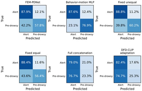
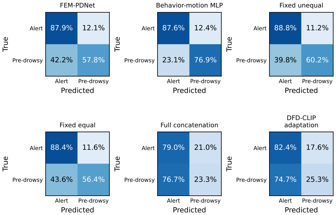
Figure 4 uses the fixed 0.5 threshold for every model, without seed ensembling or test-set threshold selection. The earlier ensemble operating point was selected using averaged outer-test predictions and is not retained as evidence of generalization. No retrospective operating point is used to improve the displayed class recalls.

Figure 4. Controlled comparison on the agreement-confirmed primary set, including DFD-CLIP at the corrected temporal learning rate. All panels use a fixed 0.5 threshold and five seeds, without probability ensembling. Cells are means of row-normalized pooled outer-test confusion matrices across seeds; each seed evaluates the same 206 clips. The repeated counts are not independent samples.

Precision and average precision (AP) are reported for the curated primary set in Table 8. AP uses the stepwise precision–recall definition, not trapezoidal integration. The primary PD proportion was $90/206=43.7\%$, whereas the PD proportion among alert/pre-drowsy clips in the final accumulated reviewed pool was $147/(1284+147)=10.3\%$. Neither proportion estimates the prevalence in real driving. To examine prevalence dependence, seed-specific positive predictive value (PPV) was calculated as

$${\mathrm{PPV}}_s\left(\pi \right)={\displaystyle \frac{\pi {\mathrm{TPR}}_s}{\pi {\mathrm{TPR}}_s+(1-\pi ){\mathrm{FPR}}_s}},$$

(22)

then summarized across seeds. At the accumulated-pool PD proportion, FEM-PDNet PPV was $0.367\pm 0.145$, compared with observed primary-set precision $0.776\pm 0.102$. Table 9 also includes 1%, 5%, and 20% as illustrative lower-prevalence scenarios, not empirical driving prevalences. Because originally alert recordings are absent and 81 of 116 clip-level alert cases come from drowsy source videos, both the observed precision/recall and these PPV scenarios concern a selected binary task rather than natural-population alert-versus-pre-drowsy screening. The calculation assumes unchanged class-conditional error rates and changes class proportions only; it does not establish deployment PPV or correct the cohort and label limitations discussed in Section 4. No independently annotated random screening sample was evaluated.

Table 8. PD precision and average precision on the curated primary set.

Model	PD Precision	Average Precision
FEM-PDNet	$0.776\pm 0.102$	$0.734\pm 0.155$
Fixed equal	$0.794\pm 0.085$	$0.759\pm 0.087$
Fixed unequal	$0.813\pm 0.077$	$0.769\pm 0.111$
Behavior–motion MLP	$0.843\pm 0.088$	$0.877\pm 0.053$
Joint-feature sensitivity	$0.825\pm 0.055$	$0.817\pm 0.071$
DFD-CLIP adaptation	$0.509\pm 0.124$	$0.515\pm 0.104$

Mean ± SD across seeds. Precision uses threshold 0.5; AP summarizes the score ranking on the curated evaluation sample. Full seed-wise metrics for all 16 configurations are in Supplementary Revision Table S1.

Table 9. Illustrative PPV under specified prevalence assumptions.

Assumed PD Prevalence	FEM-PDNet	Behavior–Motion MLP
1.00%	$0.054\pm 0.035$	$0.102\pm 0.097$
5.00%	$0.219\pm 0.111$	$0.326\pm 0.202$
10.27%	$0.367\pm 0.145$	$0.485\pm 0.205$
20.00%	$0.544\pm 0.149$	$0.652\pm 0.167$
43.69%	$0.776\pm 0.102$	$0.843\pm 0.088$

10.27% is the PD proportion among alert/pre-drowsy clips in the final accumulated reviewed pool; 43.69% is the curated primary-set PD proportion. Other values are scenarios. PPV is calculated for each seed before averaging, assuming unchanged sensitivity and specificity.

3.6. Initialization Sensitivity and Branch-Level Error Analysis

Increasing the seed count did not remove instability. Across five seeds, FEM-PDNet macro-F1 ranged from 0.557 to 0.857 and PD recall from 0.244 to 0.856. The coefficient initializations also mattered: learning from $(1,1)$ gave $0.723\pm 0.079$, whereas learning from $(0.05,0.70)$ gave $0.420\pm 0.073$. The latter contrast with FEM-PDNet remained significant after Holm adjustment ($p=0.0260$). These results describe sensitivity to the complete training initialization. The fixed-equal and learned-equal-initialization variants made the same 1030 clip–seed decisions, although their probabilities differed.

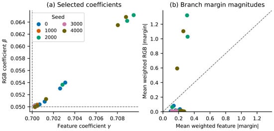
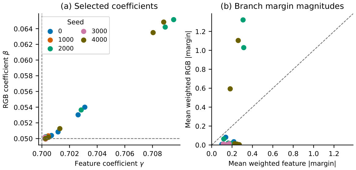
At the 25 selected FEM-PDNet checkpoints, $\gamma$ ranged from 0.700229 to 0.709531 and $\beta$ from 0.049942 to 0.065150 (Figure 5). Coefficients alone do not measure branch importance: a small coefficient can multiply a large logit margin. For class margin $m={\mathcal{l}}_{\mathrm{PD}}-{\mathcal{l}}_{\mathrm{alert}}$, the weighted RGB margin was reconstructed from saved fused probabilities and the verified frozen feature-MLP output as $\beta m^{\mathrm{video}}=\log [p_{\mathrm{PD}}/(1-p_{\mathrm{PD}})]-\gamma m^{\mathrm{feat}}$. At threshold 0.5, away from decision ties, opposing weighted margins produce the decision favored by the larger magnitude. The same mechanism can correct a feature-branch error or overturn a correct feature prediction, depending on which branch supports the assigned label. The reconstructed margin belongs to the RGB branch within the selected fusion checkpoint, not the separately trained RGB-only baseline.

Figure 5. Selected FEM-PDNet coefficients and within-model branch margins across 25 fold–seed checkpoints. (a) Coefficients relative to initialization; (b) clip-mean absolute weighted margins. Each point is a checkpoint. The diagonal in (b) denotes equal weighted-margin magnitude, not equal predictive value.

Here a correction means that fusion changes an incorrect feature-branch decision to a correct one; an introduced error is the reverse. Across all 1030 clip–seed evaluations, fusion corrected 15 and introduced 99 errors. The counts were 13 and 11 for alert clips, and two and 88 for PD clips. Eighty-five of the 99 introduced errors occurred in folds 3 and 4 at seeds 2000 and 4000. In each of these four checkpoints, the clip-mean absolute weighted RGB margin exceeded its feature counterpart. This aggregate pattern is consistent with RGB dominance in those checkpoints, but does not show that every erroneous clip had the same mechanism. The counts repeat the same 206 clips across seeds; they are not independent observations. Mechanistic interpretation and limits are consolidated in Section 4.

A separate coefficient-reset diagnostic restored $(0.70,0.05)$ at the selected checkpoints without retraining either branch. Only one decision changed, and mean macro-F1 changed from 0.718715 to 0.720125. The as-trained-minus-reset difference was $-0.001409$ (95% CI [$-0.006512$, 0]). This conditional, probability-reconstructed analysis was not added to the 16-contrast family. It tests the selected model with restored coefficients, not the entire coefficient-learning trajectory. Its relation to the fixed-weight controls is discussed in Section 4. Supplementary Revision Tables S3 and S4 provide the coefficients and diagnostic results.

Probability scores also did not establish an advantage of the selected coefficients over their restored initialization. Mean NLL was 0.647251 versus 0.639204, and Brier score was 0.227810 versus 0.223856. The as-trained-minus-reset differences were 0.008047 (95% CI [$-0.000829$, 0.026008]) and 0.003954 (95% CI [$-0.000105$, 0.012373]), respectively; lower scores are better. These proper scores describe probability prediction on the curated sample (Supplementary Revision Table S10).

Holding the branch outputs fixed separated coefficient selection from branch retraining. Development-selected grid and continuous coefficient fitting yielded macro-F1 of $0.791\pm 0.063$ and $0.787\pm 0.063$, respectively, compared with $0.720\pm 0.141$ for the initial ratio with a fitted positive scale. The continuous-minus-initial-ratio NLL difference was $-0.057053$ (95% CI [$-0.178582$, 0.013586]); its interval included zero. The matched feature-only endpoint remained higher in mean macro-F1 ($0.823\pm 0.017$); the continuous-minus-feature difference was $-0.036583$ (95% CI [$-0.114936$, 0.007038]). Continuous fitting corrected a mean of 2.6 feature errors but introduced 8.4 errors per seed, compared with 3.0 corrections and 19.8 introduced errors for the original fusion. These conditional post-hoc estimates concern coefficient selection for the same branch outputs (Supplementary Revision Table S11); their inferential limits are discussed in Section 4.

3.7. Historical Label-Scope and Non-Overlap Sensitivity

The historical reviewed-set analysis retained its original three seeds and is reported separately in Table 10. It is not an additional five-seed comparison. The older RGB + FaceMesh and equal-fusion runs included distillation, unlike their corrected primary controls; therefore, their historical rankings do not isolate architectural effects. The reviewed set adds majority-assigned cases from the original pool. The consequences of curation, repeat judgments, and agreement filtering are discussed in Section 4.

Table 10. Historical three-seed label-scope sensitivity; not the revised five-seed comparison.

Model	Primary F1	Reviewed F1	Primary PD	Reviewed PD
RGB	$0.413\pm 0.046$	$0.506\pm 0.027$	$0.122\pm 0.089$	$0.301\pm 0.057$
RGB + FaceMesh *	$0.587\pm 0.112$	$0.648\pm 0.045$	$0.341\pm 0.165$	$0.480\pm 0.104$
Concat	$0.487\pm 0.011$	$0.500\pm 0.043$	$0.241\pm 0.071$	$0.278\pm 0.120$
Equal *	$0.709\pm 0.086$	$0.710\pm 0.049$	$0.530\pm 0.180$	$0.539\pm 0.094$
FEM-PDNet	$0.744\pm 0.152$	$0.740\pm 0.087$	$0.607\pm 0.269$	$0.660\pm 0.172$

Primary/reviewed denote the 206-/256-clip sets; PD denotes recall. * Historical RGB + FaceMesh and equal fusion included distillation and are not the corrected no-distillation controls. All entries retain the historical seeds 0, 1000, and 2000 and are excluded from the new Holm family.

The strict non-overlap analysis is reported as a secondary result while retaining its post-hoc status (Table 11). Clips were sorted within each source video by end time, start time, and identifier; a clip was retained only if its start was at or after the end of the previously retained clip. The deterministic rule used neither class labels nor model outputs. It removed 14 clips (one alert and 13 PD), reduced overlapping pairs from 21 to zero, and retained all 51 subjects. FEM-PDNet was retrained with the same five folds, three historical seeds, checkpoint rule, and other architectural/optimization settings. Class weights and feature-preprocessing statistics were recomputed on the retained training subjects in each fold.

Table 11. Historical matched three-seed non-overlap retraining sensitivity.

Analysis Set	n (Alert/PD)	Overlap Pairs	Macro-F1	PD Recall
Agreement-confirmed	206 (116/90)	21	$0.744\pm 0.152$	$0.607\pm 0.269$
Strict non-overlap	192 (115/77)	0	$0.765\pm 0.065$	$0.654\pm 0.126$

Both sets retain 51 subjects and five outer folds. Values are mean ± SD across the original three seeds at threshold 0.5. This post-hoc sensitivity does not replace the primary analysis or imply improved generalization.

Macro-F1 was $0.765\pm 0.065$ and PD recall $0.654\pm 0.126$ on the 192-clip subset, compared with $0.744\pm 0.152$ and $0.607\pm 0.269$ in the matched three-seed 206-clip analysis. These estimates are similar in magnitude; they neither demonstrate improvement nor isolate the causal effect of overlap removal, because class composition and training examples also changed. Temporal overlaps already remained within each subject-disjoint partition (Section 2.1); this analysis removes repeated windows within partitions.

3.8. Processing Time and Memory

An isolated post-hoc benchmark used the five seed-0 checkpoints for each configuration and the same 50 clips, selected by an identifier-hash rule without labels or predictions (10 per fold). Each fold used three warm-up clips and three timed repetitions per selected clip. Measurements used one clip per batch, FP32 without AMP/TF32, synchronized CUDA, sequential model/fold processes, and one Torch/OpenCV CPU thread; these settings do not fix MediaPipe’s internal thread count. Saved-probability replay checked the native evaluation path within ${10}^{-6}$, and fresh preprocessing was checked against a separate condition-matched batch-1 reference within $2\times {10}^{-5}$, with no decision changes. Cross-condition probability differences were recorded separately rather than treated as numerical parity.

Frame-file pipeline time includes JPEG reading/decoding, model-specific transforms, fresh FaceMesh and motion extraction where applicable, saved training-split preprocessing, transfers, and prediction. Model-only time starts with prepared device-resident tensors and includes softmax and clip aggregation. Neither measurement includes raw source-video decoding, initial frame-cache creation, camera capture, the 8 s observation interval, or model initialization. File caches were warm after input hashing. This is not a live-camera end-to-end or embedded-device benchmark.

FEM-PDNet required 327.47 ms per clip on average for the frame-file pipeline (95th percentile 342.98 ms), compared with 8.64 ms for model-only inference. FaceMesh extraction averaged 234.94 ms, approximately 71.7% of pipeline time; optical-flow/frame-difference extraction averaged 25.23 ms. Thus, feature extraction, rather than the two scalar coefficients, dominated the measured pipeline cost. The behavior–motion MLP required 267.93 ms for the pipeline despite only 0.32 ms for model inference. Similar weighted-fusion latencies do not demonstrate real-time feasibility under vehicle operating conditions.

FEM-PDNet contained 12,628,391 PyTorch parameters, of which 1,446,917 were trainable in its fusion stage. Its sampled pipeline CPU resident-set peak was 1517.25 MiB, with PyTorch allocated/reserved GPU peaks of 509.98/528.00 MiB. CPU sampling at 5-ms intervals can miss brief peaks and includes the process/runtime; it is not total system memory. GPU figures exclude driver and non-PyTorch allocations. Parameter counts exclude the separate FaceLandmarker task, although its runtime and process memory are included. Parameter, trainability, and memory measurements are in Supplementary Revision Table S5; stage timings are in the accompanying aggregate CSVs. The 150 timing calls per model are repeated measurements, not 150 independent clips. The per-clip processing-time measurements are summarized in Table 12.

Table 12. Post-hoc processing time per clip in milliseconds.

Model	Pipeline Mean	Pipeline p95	Model-Only Mean
FEM-PDNet	327.47	342.98	8.64
Fixed equal	327.39	337.67	8.63
Fixed unequal	328.42	339.06	8.64
Behavior–motion MLP	267.93	272.34	0.32
RGB only	57.24	67.65	8.15
RGB + FaceMesh	298.30	305.88	8.63
Full concatenation	327.61	338.67	8.64
Distillation sensitivity	328.26	341.79	8.65
Eye-Region CNN	41.14	57.62	0.33
ViT Frame	8.71	9.24	7.50
CNN-LSTM Temporal	23.13	25.35	0.34
Learned init. (1, 1)	327.94	341.78	8.64
Learned init. (0.05, 0.70)	328.57	343.11	8.68
Joint-feature sensitivity	328.34	342.54	8.65
FastKAN-DDD adaptation	23.41	26.42	0.47
DFD-CLIP adaptation	23.74	25.15	12.56

A total of 50 common clips, three timed repeats each, seed-0 checkpoints from five folds. Pipeline starts from existing frame files, not source video or camera acquisition. p95 summarizes 150 timed calls per configuration. The DFD-CLIP timing row was measured with the historical R1 checkpoints. It is not a measurement of the learning-rate-corrected checkpoints.

4. Discussion and Limitations

The principal findings are mixed: fusion differed from the tested concatenation implementation, but matched fixed-weight controls did not demonstrate an additional benefit from optimizing coefficients, and the behavior–motion MLP had higher mean macro-F1 than FEM-PDNet. These are distinct empirical questions. A gain over one integration implementation cannot be attributed automatically to coefficient learning or an incremental RGB contribution. Nonsignificant fixed-weight contrasts also do not establish equivalence.

The within-model diagnostics explain how RGB can reduce performance without establishing why its predictions generalize poorly. For the binary task, fusion uses $m=\gamma m^{\mathrm{feat}}+\beta m^{\mathrm{video}}$. When the feature margin supports the assigned label but the RGB term has the opposite sign and larger weighted magnitude, fusion reverses a correct feature decision. A small $\beta$ does not prevent this because raw logit scales can differ. Introduced errors exceeded corrections, predominantly among PD-labeled clips, and 85 of 99 introduced errors were concentrated in four fold–seed checkpoints. This is observed decision behavior, not a causal experiment on illumination, background, occlusion, encoder choice, or sample size. The separately trained MLP comparison and the copied feature-branch diagnostic are reported separately.

The behavior–motion features also closely match the visible cues used to assign the operational labels, which makes their strong performance consistent with the task definition rather than independent evidence of physiological validity. The RGB branch need not supply additional useful information for this particular target. This does not establish that RGB is generally detrimental in driver monitoring. Identifying environmental or architectural causes would require independently controlled data or interventions, neither of which was performed here.

Initialization affected the complete fusion training trajectory, and joint-feature training had a higher mean without an established improvement under the family-adjusted analysis. Restoring initial coefficients changed only one thresholded decision. These results do not demonstrate convergence to a uniquely beneficial learned weighting rule or justify a prospective branch-selection policy.

The same-branch analysis holds the representations fixed. Refitting the ratio reduced mean introduced feature errors but remained below the feature-only mean score. Grid and continuous fitting gave similar estimates, and the continuous-minus-initial-ratio NLL interval included zero. Positive scale fitting changes probability confidence, not fixed-0.5 decisions at a given ratio. NLL and Brier comparisons are proper-score analyses of this selected class distribution, not calibration-only tests or deployment-prevalence estimates. The checkpoint-selection subjects were reused for conditional development fitting; no independent calibration set was evaluated. These post-hoc diagnostics do not replace the primary comparisons or establish a unique advantage of gradient-based weighting.

The target remains an operational visual state. Annotation and feature extraction quantify overlapping eye, mouth, gaze, head, and motion cues; this construct overlap is distinct from train–test leakage. Subject-disjoint partitions do not validate a physiological pre-drowsiness condition or a prospective warning event. Moderate agreement and agreement filtering may favor clearer cases. Original labels are coarse, predominantly self-reported video states, not ground truth for every interval. The annotators had AI backgrounds, no joint rubric review or practice calibration, and no independently documented single rubric version fixed before all rounds. Same-day repeated judgments by B may be affected by recall; saved decision paths lack per-pass behavioral rationales. The reviewed-set sensitivity therefore does not resolve label validity or demonstrate that filtering has no effect.

The curated 206 clips from 51 subjects provide limited coverage; additional seeds measure optimization variation without adding subjects. No originally alert recordings are represented, and 81 of 116 clip-level alert cases come from drowsy source videos. This is not itself evidence of incorrect interval labels, but the resulting case spectrum differs from natural-population alert-versus-pre-drowsy screening. Precision, recall, and AP are conditional on this selection. PPV reweighting assumes unchanged class-conditional error rates and cannot restore absent source categories, alter case difficulty, or remove readability selection and domain shift. The non-overlap subset reduces repeated windows but retains the source population. Indoor recordings do not test moving-vehicle illumination, occlusion, vibration, camera placement, or outdoor conditions. Deployment relevance therefore requires independently annotated, representative external/on-road data.

All comparisons are conditional retrospective evidence on an adaptively curated, previously inspected cohort. Earlier model errors influenced some re-review target selection; blindness during relabeling and subject-disjoint cross-validation do not make that cohort untouched. The locked revision plan limits subsequent analytical changes but does not erase prior exposure. Five seeds do not provide five independent cohorts, marginal bootstrap intervals are not family-adjusted intervals, and resampling saved outputs does not account for all training-cohort uncertainty. Baseline pretraining and task adaptations remain disclosed, and derived annotation/evaluation resources have review-only access rather than a public release. The complete comparison family and negative findings are retained; none of these procedures supplies independent external confirmation of generalization.

5. Conclusions

This study provides retrospective comparisons of fixed and learned RGB/behavior–motion fusion on an adaptively curated UTA-RLDD cohort. The operational visual-state labels are not independent physiological measurements or prospective early-warning outcomes. Matched fixed-weight controls did not demonstrate an additional benefit of learning coefficients, and the behavior–motion MLP had higher mean macro-F1 than FEM-PDNet. RGB corrected some feature errors but introduced more, illustrating that fusion can reduce performance when conflicting weighted margins dominate. Initialization and conditional same-branch analyses further characterized this sensitivity without establishing a superior weighting or branch-selection rule. These negative and mixed findings are central results, not evidence of universally beneficial fusion. Subject-disjoint evaluation on this previously inspected cohort, whose clips exclude originally alert recordings, does not independently establish natural-population screening performance or real-driving generalization.

References

- Korea Road Traffic Authority. Caution Against Spring Drowsy-Driving Traffic Accidents: Fatality Rate Approximately Twice That of All Traffic Accidents [Translated from Korean]. 2025. Available online: https://www.koroad.or.kr/main/board/6/302605/board_view.do?bdNoticeYn=N&bdOpenYn=Y&listType=list (accessed on 1 July 2026). (In Korean)
- Sahayadhas, A.; Sundaraj, K.; Murugappan, M. Detecting driver drowsiness based on sensors: A review. Sensors 2012, 12, 16937–16953, Correction in Sensors 2021, 21, 451. https://doi.org/10.3390/s121216937. [Google Scholar] [CrossRef] [Scilit]
- Sikander, G.; Anwar, S. Driver fatigue detection systems: A review. IEEE Trans. Intell. Transp. Syst. 2019, 20, 2339–2352. [Google Scholar] [CrossRef] [Scilit]
- Lal, S.K.L.; Craig, A. A critical review of the psychophysiology of driver fatigue. Biol. Psychol. 2001, 55, 173–194. [Google Scholar] [CrossRef] [Scilit]
- Åkerstedt, T.; Gillberg, M. Subjective and objective sleepiness in the active individual. Int. J. Neurosci. 1990, 52, 29–37. [Google Scholar] [CrossRef] [Scilit]
- Johns, M.W. A new method for measuring daytime sleepiness: The Epworth Sleepiness Scale. Sleep 1991, 14, 540–545. [Google Scholar] [CrossRef] [Scilit]
- Healey, J.A.; Picard, R.W. Detecting stress during real-world driving tasks using physiological sensors. IEEE Trans. Intell. Transp. Syst. 2005, 6, 156–166. [Google Scholar] [CrossRef] [Scilit]
- Dong, Y.; Hu, Z.; Uchimura, K.; Murayama, N. Driver inattention monitoring system for intelligent vehicles: A review. IEEE Trans. Intell. Transp. Syst. 2011, 12, 596–614. [Google Scholar] [CrossRef] [Scilit]
- The Technology Division of Federal Motor Carrier Safety Administration in United States. PERCLOS: A Valid Psychophysiological Measure of Alertness as Assessed by Psychomotor Vigilance; Tech Brief FHWA-MCRT-98-006; United States Federal Motor Carrier Safety Administration: Washington, DC, USA, 1998. [Google Scholar] [CrossRef]
- Ji, Q.; Zhu, Z.; Lan, P. Real-time nonintrusive monitoring and prediction of driver fatigue. IEEE Trans. Veh. Technol. 2004, 53, 1052–1068. [Google Scholar] [CrossRef] [Scilit]
- Bergasa, L.M.; Nuevo, J.; Sotelo, M.A.; Barea, R.; Lopez, M.E. Real-time system for monitoring driver vigilance. IEEE Trans. Intell. Transp. Syst. 2006, 7, 63–77. [Google Scholar] [CrossRef] [Scilit]
- McDonald, A.D.; Lee, J.D.; Schwarz, C.; Brown, T.L. A contextual and temporal algorithm for driver drowsiness detection. Accid. Anal. Prev. 2018, 113, 25–37. [Google Scholar] [CrossRef] [Scilit]
- Deng, W.; Wu, R. Real-time driver-drowsiness detection system using facial features. IEEE Access 2019, 7, 118727–118738. [Google Scholar] [CrossRef] [Scilit]
- Abtahi, S.; Hariri, B.; Shirmohammadi, S. Driver drowsiness monitoring based on yawning detection. In Proceedings of the 2011 IEEE International Instrumentation and Measurement Technology Conference, Hangzhou, China, 10–12 May 2011; pp. 1–4. [Google Scholar] [CrossRef] [Scilit]
- Abtahi, S.; Omidyeganeh, M.; Shirmohammadi, S.; Hariri, B. YawDD: A yawning detection dataset. In Proceedings of the 5th ACM Multimedia Systems Conference, Singapore, 19 March 2014; pp. 24–28. [Google Scholar] [CrossRef] [Scilit]
- Massoz, Q.; Langohr, T.; François, C.; Verly, J.G. The ULg multimodality drowsiness database (called DROZY) and examples of use. In Proceedings of the 2016 IEEE Winter Conference on Applications of Computer Vision, Lake Placid, NY, USA, 7–10 March 2016; pp. 1–7. [Google Scholar] [CrossRef] [Scilit]
- Park, S.; Pan, F.; Kang, S.; Yoo, C.D. Driver drowsiness detection system based on feature representation learning using various deep networks. In Proceedings of the Computer Vision—ACCV 2016 Workshops, LNCS 10118; Springer: Cham, Switzerland, 2017; pp. 154–164. [Google Scholar] [CrossRef] [Scilit]
- Wijnands, J.S.; Thompson, J.; Nice, K.A.; Aschwanden, G.D.P.A.; Stevenson, M. Real-time monitoring of driver drowsiness on mobile platforms using 3D neural networks. Neural Comput. Appl. 2020, 32, 9731–9743. [Google Scholar] [CrossRef] [Scilit]
- Yu, J.; Park, S.; Lee, S.; Jeon, M. Driver drowsiness detection using condition-adaptive representation learning framework. IEEE Trans. Intell. Transp. Syst. 2019, 20, 4206–4218. [Google Scholar] [CrossRef] [Scilit]
- Lyu, J.; Yuan, Z.; Chen, D. Long-term multi-granularity deep framework for driver drowsiness detection. arXiv 2018, arXiv:1801.02325. [Google Scholar] [CrossRef] [Scilit]
- Jabbar, R.; Al-Khalifa, K.; Kharbeche, M.; Alhajyaseen, W.; Jafari, M.; Jiang, S. Real-time driver drowsiness detection for Android application using deep neural networks techniques. Procedia Comput. Sci. 2018, 130, 400–407. [Google Scholar] [CrossRef] [Scilit]
- Simonyan, K.; Zisserman, A. Two-stream convolutional networks for action recognition in videos. In Proceedings of the Advances in Neural Information Processing Systems; NeurIPS: San Diego, CA, USA, 2014; Volume 27, pp. 568–576. [Google Scholar]
- King, D.E. Dlib-ml: A machine learning toolkit. J. Mach. Learn. Res. 2009, 10, 1755–1758. [Google Scholar]
- Ghoddoosian, R.; Galib, M.; Athitsos, V. A realistic dataset and baseline temporal model for early drowsiness detection. In Proceedings of the2019 IEEE/CVF Conference on Computer Vision and Pattern Recognition Workshops (CVPRW), Long Beach, CA, USA, 16–17 June 2019; pp. 178–187. [Google Scholar] [CrossRef] [Scilit]
- Essahraui, S.; Lamaakal, I.; Maleh, Y.; El Makkaoui, K.; Filali Bouami, M.; Ouahbi, I.; Elmannai, H.; Abd El-Latif, A.A. FastKAN-DDD: A Novel Fast Kolmogorov-Arnold Network-Based Approach for Driver Drowsiness Detection Optimized for TinyML Deployment. PLoS ONE 2025, 20, e0332577, Correction in PLoS ONE 2026, 21, e0340596. https://doi.org/10.1371/journal.pone.0332577. [Google Scholar] [CrossRef] [Scilit]
- Bai, J.; Fu, X.; Zhu, G.; Wu, L.; You, J.; Gao, Y.; Kwong, S. DFD-CLIP: A Unified Vision-Language Framework for Driving Fatigue Detection with Temporal Modeling and Adaptive Prompt Learning. IEEE Trans. Multimed. 2026, 28, 10460–10474. [Google Scholar] [CrossRef] [Scilit]
- He, K.; Zhang, X.; Ren, S.; Sun, J. Deep residual learning for image recognition. In Proceedings of the 2016 IEEE Conference on Computer Vision and Pattern Recognition (CVPR), Las Vegas, NV, USA, 27–30 June 2016; pp. 770–778. [Google Scholar] [CrossRef] [Scilit]
- Cho, K.; van Merriënboer, B.; Gulcehre, C.; Bahdanau, D.; Bougares, F.; Schwenk, H.; Bengio, Y. Learning phrase representations using RNN encoder–decoder for statistical machine translation. In Proceedings of the 2014 Conference on Empirical Methods in Natural Language Processing (EMNLP), Doha, Qatar, 25–29 October 2014; pp. 1724–1734. [Google Scholar] [CrossRef] [Scilit]
- Lugaresi, C.; Tang, J.; Nash, H.; McClanahan, C.; Uboweja, E.; Hays, M.; Zhang, F.; Chang, C.L.; Yong, M.G.; Lee, J.; et al. MediaPipe: A framework for building perception pipelines. arXiv 2019, arXiv:1906.08172. [Google Scholar] [CrossRef] [Scilit]
- Kartynnik, Y.; Ablavatski, A.; Grishchenko, I.; Grundmann, M. Real-time facial surface geometry from monocular video on mobile GPUs. arXiv 2019, arXiv:1907.06724. [Google Scholar] [CrossRef] [Scilit]
- Farnebäck, G. Two-frame motion estimation based on polynomial expansion. In Proceedings of the Image Analysis—SCIA 2003, LNCS 2749; Springer: Berlin/Heidelberg, Germany, 2003; pp. 363–370. [Google Scholar] [CrossRef] [Scilit]
- Bradski, G. The OpenCV Library. Dr. Dobb’s J. Softw. Tools 2000, 25, 122–125. [Google Scholar] [CrossRef] [Scilit]
- Horn, B.K.P.; Schunck, B.G. Determining optical flow. Artif. Intell. 1981, 17, 185–203. [Google Scholar] [CrossRef] [Scilit]
- Dosovitskiy, A.; Beyer, L.; Kolesnikov, A.; Weissenborn, D.; Zhai, X.; Unterthiner, T.; Dehghani, M.; Minderer, M.; Heigold, G.; Gelly, S.; et al. An image is worth 16×16 words: Transformers for image recognition at scale. In Proceedings of the International Conference on Learning Representations, Virtual, 3–7 May 2021. [Google Scholar]
Disclaimer/Publisher’s Note: The statements, opinions and data contained in all publications are solely those of the individual author(s) and contributor(s) and not of MDPI and/or the editor(s). MDPI and/or the editor(s) disclaim responsibility for any injury to people or property resulting from any ideas, methods, instructions or products referred to in the content. |
© 2026 by the authors. Licensee MDPI, Basel, Switzerland. This article is an open access article distributed under the terms and conditions of the Creative Commons Attribution (CC BY) license.