Adjacent Cell Score for Mobile Sink Placement Using Deep Q Net-Based Energy Prediction in WSN

Abstract

In recent years, Wireless Sensor Networks (WSNs) have been widely adopted in healthcare, manufacturing, military, environmental monitoring, and other applications. Because sensor nodes have limited energy, multi-hop communication can create energy-hole regions around the sink. This paper proposes a mobile-sink placement framework that combines Voronoi partitioning, Deep Embedded Clustering (DEC), an adjacency-based cell score, and a Deep Q-Network (DQN) for energy prediction. The network is first partitioned into Voronoi cells, and DEC is used consistently for Cluster Head (CH) selection. For each candidate sink cell, the adjacency-based cell score considers distance, fairness, and predicted residual energy. DQN is used to predict residual energy from a defined WSN state representation, while the DQN agent is trained at the Base Station (BS); sensor nodes are not required to execute the neural network. The reported simulations consider 100, 200, 300, and 400 nodes over 2000 rounds. In the comparative table, the proposed method reports a minimum distance of 21 m for the 400-node case, residual energy of 0.746 J, normalized fairness of 95, network lifetime of 89 s, and normalized throughput of 96 for the corresponding reported case. The study focuses on placement optimization and does not model mobile-sink travel energy, speed, or collection latency; these are identified explicitly as limitations and future extensions.

1. Introduction

The great number of low-cost sensors that are compactly and randomly organized in the region to be monitored is called the sensor network [1]. WSN comprises numerous mobile as well as static sensors that are arranged in a multi-hop self-organizing fashion [2]. WSN includes numerous nodes and comprises several data collection points called sinks. In general, sensor nodes are very small electronic components with minimal resources, such as processing energy and memory [3]. Moreover, in order to collect precise data through multi-hop interaction with the Base Station (BS), such nodes are constructed frequently. The main purpose of the sink node is to receive the collected information [4]. Every WSN is constrained by low data rates, energy reservations, and usually a many-to-one communication pattern [5]. Wireless sensor networks have attracted significant attention because of the large number of new applications in home automation, environmental monitoring, military operations, health services, and other commercial environments [6]. A WSN which optimizes energy usage and provides high system performance must be planned by the network designer based on various criteria. Furthermore, distinctive circumstances for large-scale WSNs comprise multiple sinks and multiple sources. Compared to a single sink, multiple sinks provide better manageability for WSNs [7].

In WSN, the terminal node forwards the information to the sink node through multi-hop [8]. However, multi-hop data transmission causes an energy hole. As the nodes situated around the sinkhole take many tasks to forward the data, the nodes may exhaust or consume a lot of energy, and this will damage the network connectivity in WSN [9]. Due to the collision caused by frequent data transmission and communication between nodes, the multi-hop transmission produces communication overhead [10]. Initially, mobile sinks are utilized for determining the optimal sink location. Afterwards, the stationary sinks are employed for gathering data packets from sensor nodes by multi-hop communication. When sinks and sensor nodes are improperly deployed, it becomes hard to manage an operational network, which has an adverse effect on system performance and energy consumption. For a random-based deployment process of a WSN, the sink placement becomes an important criterion for the network designer to increase the network lifetime and system [11]. One way to balance the load over the network is to deploy more nodes in areas closer to the sink [12]. Achieving maximum lifetime in stationary WSNs by optimally using the energy within sensor nodes has been the subject of significant research in recent years [13]. Furthermore, the main difficulty is in estimating the optimal location of BS. Here, the distribution of WSNs is executed in a structured or planned method in a semi-random pattern [14].

Wireless Sensor Network (WSN) is an emerging and exigent technology being used in various applications such as health monitoring, GPS tracking, security, environmental monitoring, etc. In WSN, numerous cost-effective and energy-constrained sensor nodes are typically used. The mobile sinks gather the information from the sensors deployed in the environment periodically, in such a way to avoid the energy-crisis and hotspot issues. Moreover, the use of mobile sinks in a WSN can effectively improve the network performance, and it has been exploited in numerous schemes to prolong the lifetime of WSNs. In this work, an effective strategy is developed to detect the location of a mobile sink and energy prediction of WSN. The optimal placement of the mobile sink is achieved using the adjacency-based cell score in such a way that the lifespan of the network is extended and the energy consumed by the nodes is reduced based on factors such as the location of the sink, fairness, energy, and Euclidean distance.

This work implements a method for mobile sink placement using the proposed Deep Learning (DL) method-based energy prediction in WSN. The cell network is transformed by Voronoi partition and then various clusters are formed. From each cluster, the CH is selected utilizing DEC. Then, the location of the mobile sink is identified based on the adjacency-based cell score computed using several factors, such as distance, fairness, and predicted energy. The Deep Q Net is employed for energy prediction.

The contribution of the work is mentioned below,

• Optimized Mobile Sink Placement using Deep Q Net: The proposed model utilizes Deep Q Net for the optimal placement of mobile sinks in Wireless Sensor Networks (WSN), ensuring that the mobile sink is strategically positioned to extend the network’s lifetime and reduce the energy-hole problem effectively.
• Cluster Formation with Voronoi Partition and Deep Embedded Clustering: The approach incorporates Voronoi partitioning to transform the cell network and divides it into various clusters. It also employs Deep Embedded Clustering (DEC) for the efficient selection of Cluster Heads (CH), enhancing data collection and energy efficiency within the WSN.
• Enhanced Network Performance Metrics: The work presents a novel approach for optimizing the placement of mobile sinks in Wireless Sensor Networks (WSNs) using Deep Q Net. By employing Voronoi partitioning to transform the network into clusters and leveraging Deep Embedded Clustering (DEC) for Cluster Head (CH) selection, the approach ensures efficient data collection and enhanced energy management.

The organization of the residual sections is mentioned in Part 2, which elucidates existing techniques for mobile sink placement in the WSN network. Part 3 elaborates on the proposed work, its outcome along with the analysis is discussed in Part 4, and lastly, the conclusion is elaborated in Part 5.

2. Motivation

Wireless Sensor Networks (WSNs) have become increasingly vital in various applications, such as environmental monitoring, healthcare, military operations, and industrial automation. A significant challenge in WSNs is the “energy-hole problem,” where sensor nodes closer to the sink deplete their energy more rapidly than those farther away, leading to early network failure and reduced overall network lifetime. Mobile sinks offer a promising solution to this issue by relocating dynamically to balance energy consumption among nodes. However, achieving optimal placement of mobile sinks is complex and challenging. Many existing techniques rely on heuristic or static strategies that fail to adapt to the dynamic nature of WSNs, leading to suboptimal sink positions, uneven energy use, and limited network efficiency. Additionally, some methods are too complex or do not scale well, making them impractical for real-world applications. Moreover, these techniques often inadequately account for the changing conditions within the network, such as varying node energy levels and fluctuating topologies, further complicating the placement process. This research is motivated by the need to address these challenges by developing a robust and adaptive approach for mobile sink placement. By leveraging advanced techniques like Deep Q Net, Voronoi partitioning, and Deep Embedded Clustering (DEC), this work aims to ensure that mobile sinks are positioned optimally, reducing energy consumption and significantly extending network lifetime, thereby overcoming the limitations of existing methods.

Literature Review

Before exploring the proposed solution, it is crucial to review the existing literature on mobile sink placement in Wireless Sensor Networks (WSNs). Numerous strategies have been developed to address the energy-hole problem and extend network lifetime, yet many fall short in adapting to the dynamic nature of WSNs. This review will examine these methods, highlighting their limitations and the gaps that motivate the need for more robust and adaptive solutions.

Recent deep reinforcement learning methods also include continuous-action approaches such as Deep Deterministic Policy Gradient (DDPG), Proximal Policy Optimization (PPO), and Soft Actor-Critic (SAC). These methods are relevant when the action is a continuous control variable, such as a two-dimensional sink coordinate. In the present study, the decision process is formulated around a finite set of candidate cells generated by the Voronoi partition, and the DQN is used for discrete energy-prediction actions. Therefore, DDPG, PPO, and SAC are not treated as directly equivalent baselines in the current experiments. Their applicability to continuous sink-coordinate optimization is discussed as an important extension rather than claiming that the present DQN formulation is universally superior.

Kaur, C., et al. [1] introduced Deep Maxout Network (DMN) to detect the position of the mobile sink. It solved the optimization issues and enhanced the performance and network lifetime. However, it was unsuccessful in ensuring the upper bound of the estimation ratio. A tree-based heuristic data dissemination method called Tuft was devised by Busaileh, O., et al. [10] for increasing the regularity of energy consumption in a network. This method increased the success ratio and network lifetime was prolonged in all situations. Nevertheless, it suffered from high energy consumption and time complexity. Ref. [11] developed an Integer Linear Programming (ILP) for Energy and Environment-Aware Path Planning in WSN. This technique was more effective and the delivery time was shorter. However, it took more computation time as this method required more realistic parameters. The dynamic Mobility and Energy Aware Algorithm (DMEAAL) technique was presented by Kumar et al. [12] for balancing the energy consumption across individual nodes. This approach was successful in both controlling and forming grid networks, which improved the lifetime of the network. Nevertheless, there was no guarantee to energy at the same rate, and this approach failed to perform in practical applications. Ref. [15] Karpurasundharapondian et al. reviewed optimization-based clustering and routing techniques to improve energy efficiencsy in (WSNs). Their study compared various optimization algorithms and identified future research directions for enhancing routing performance and network lifetime.

Lillicrap et al. [16] introduced a dynamic mobile sink node moving path planning algorithm (DPPMSBT) for intensive WSN in order to collect the periodic data from the whole network. It generated the burst data from a single area. It gained more advantage in terms of packet loss rate, network lifetime, and path length. It degraded the performance in terms of dropped packets. Schulman et al. [17] developed a mobile sink-based energy-aware clustering (MSEAC) protocol to solve the issues of energy hole in order to increase the lifetime of the network. It outperformed the existing methods in terms of residual energy, packet delivery ratio, delay, and lifespan of the network.

Haarnoja, T. et al. [18] developed a model called multi-objective particle swarm optimization (MOPSO) for mobile sink placement. This method was used to select the best global and local solutions in the search space, which offered better results in statistical significance. The optimization of multiple mobile sinks was the major drawback of this method. Mnih, V. et al. [19] proposed a method to determine the path determination of mobile sink based on Ant Colony Optimization (ACO). This method offered better results in energy consumption and network lifetime. In any case, handling of multiple mobile sinks with non-uniform data constraints was difficult.

Saunh Sutton [20] developed an optimization algorithm, called Differential Moth Flame Optimization (DMFO), in which traversal strategy was used for the mobile sink placement. This method offered better results in energy consumption and network lifetime but failed to calculate the data latency and throughput. Elie T. Fute et al. [21] proposed an instantaneous clustering algorithm (ICP) for the determination of the target points from the mobile sink. The main aim of this method was to reduce the clustering time and increasing the network’s lifetime. The communication overhead was the major disadvantage of this method.

Challenges noted from the review are listed below.

In [10], the Tuft method was effective in reducing energy consumption and maintaining a stable network lifetime. However, it faced challenges with a decreased success ratio and high delivery delays, which resulted in increased overhead costs. The Integer Linear Programming (ILP) approach described in [11] was praised for its reliability, energy efficiency, and applicability in real-time applications, achieving environment-aware routing. Nonetheless, it struggled with ensuring consistent data transmission, which contributed to increased end-to-end delays. The Dynamic Mobility and Energy Aware Algorithm (DMEAAL) presented in [12] demonstrated enhanced efficiency, but it was prone to delays and data loss. Additionally, nodes were unable to implement the DMEAAL approach effectively until the message was fully established. Despite various approaches being employed for mobile sink placement to minimize energy consumption and reduce communication delays, existing methods often fell short in delivering precise performance.

3. Proposed Deep Q Net-Based Energy Prediction for Mobile Sink Placement in WSN

To place the mobile sink optimally in WSN without degrading the network lifetime and energy consumption poses a major challenging task. Hence, an adjacency-based cell score is formed in this research to perform the mobile sink placement optimally. Initially, the nodes are simulated in the WSN and they are transformed into the cell. This part describes the Deep Q Net-based energy prediction for the placement of the mobile sink in WSN.

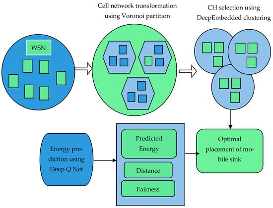
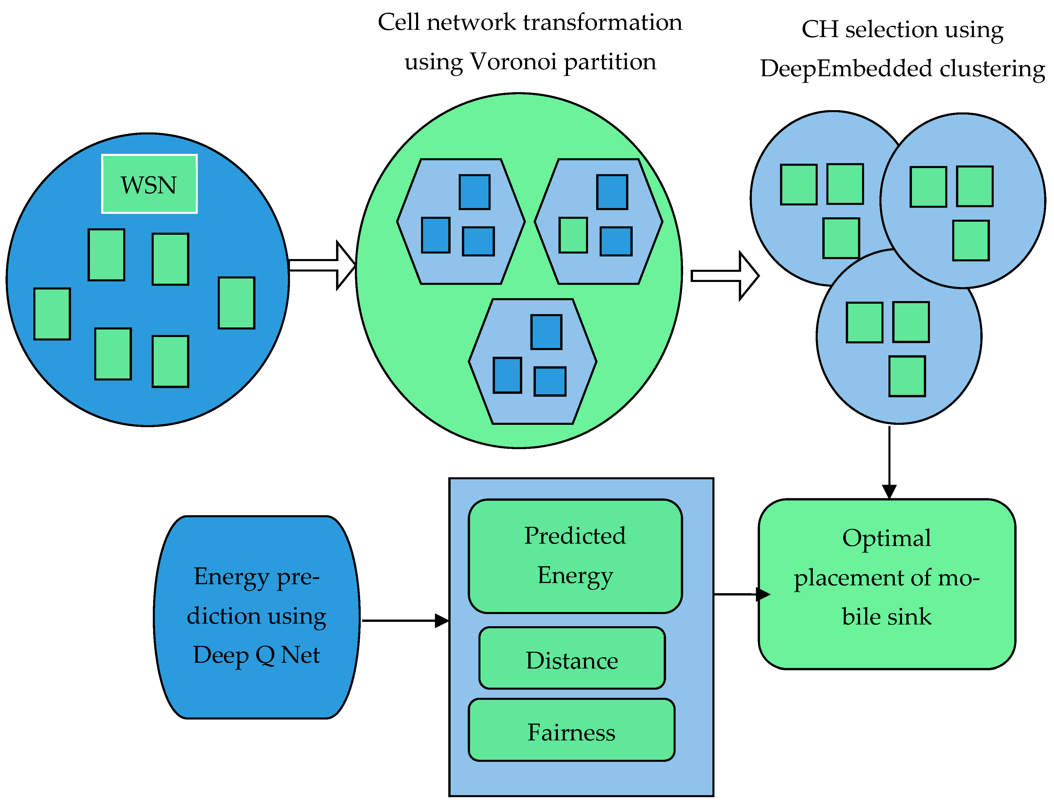
The developed model follows four stages. First, the sensor nodes are transformed into Voronoi cells. Second, Deep Embedded Clustering (DEC) is applied consistently to the cell/node features to identify Cluster Heads (CHs). Third, an adjacency-based cell score is calculated for candidate mobile-sink locations using distance, fairness, and DQN-predicted residual energy. Fourth, the candidate with the highest cell score is selected as the mobile-sink location. No FCM or sparse-FCM operation is used in the final methodology; the reference to sparse FCM in the previous version was an editorial inconsistency and has been removed. Block diagram of Deep Q Net-based energy prediction model for mobile sink placement in WSN is represented in Figure 1.

Figure 1. Block diagram of Deep Q Net-based energy prediction model for mobile sink placement in WSN.

Table 1 presents the list of abbreviations used throughout the manuscript.

Table 1. List of abbreviations.

WSN	Wireless Sensor Networks
CH	Cluster Head
DEC	Deep Embedded Clustering
DL	Deep Learning
DMN	Deep Maxout Network
ILP	Integer Linear Programming
BS	Base Station
DMEAAL	Dynamic Mobility and Energy Aware Algorithm
KL	Kullback–Leibler

3.1. Transformation of Cell Network Using Voronoi Partition

Nodes in WSN are primarily clustered to transform the nodes in the cell network. Moreover, Voronoi partition is utilized to transform the simulated nodes into different cells. The Voronoi partition is chiefly employed for optimal division of cells in WSN. The clusters of different cell regions are signified as P_m, where, m ∈ (1 ≤ m ≤ q), and q stands for the count of divided cell regions in WSN. These divided cell regions are formed based on nodes like M₁, M₂, M₃ …… M_l. Once the transformation of the cell network is accomplished, and the transformed cell is exposed to the CH selection process.

3.2. Deep Embedded Clustering for Effective CH Selection

DEC [13] is commonly utilized because of its improved performance and scalability. Moreover, DEC comprises two stages, like parameter initialization and parameter optimization. In parameter initialization, deep autoencoder is employed, whereas in parameter optimization, an iterative process is performed among the Kullback–Leibler (KL) divergence and auxiliary target distribution. Here, a group of ${\left\{d_z\in N\right\}}_{z=1}^d$ is partitioned into t clusters, and is described through a cluster centroid $y_{c^{\prime }},c^{\prime }$ = 1, …, t. To change the data latent feature space S, DEC employs non-linear mapping v_ϕ: N → S, where learnable parameters are represented as ϕ, and DNN is utilized to parameterize v_ϕ.

Clustering with KL Divergence

An unsupervised approach exchanges between two stages, and is utilized for enhancing the clustering with a value of ϕ and ${\left\{y_{c^{\prime }}\right\}}_{c^{\prime }=1}^t$. In first stage, soft assignment is assessed among embedded points and cluster centroids. In second stage, deep mapping v_ϕ is updated and high-confidence assignments are learned by employing auxiliary target distribution. Moreover, these two stages are performed repeatedly until convergence is obtained.

(a)

Soft assignment

To determine the relations among centroid $y_{c^{\prime }}$ and embedded point $g_{c^{\prime }}^{\prime }$, the student’s t-distribution is used, which is demonstrated as

$$r_{c^{\prime }z}^{\prime }={\displaystyle \frac{{\left(1+{‖g_z^{\prime }-y_{c^{\prime }}‖}^2/\mathsf{\gamma }\right)}^{-\frac{\mathsf{\gamma }+1}{2}}}{{\displaystyle {\sum }_{i^{\prime }}{\left(1+{‖{g^{\prime }}_z-y_{c^{″}}‖}^2/\mathsf{\gamma }\right)}^{-\frac{\mathsf{\gamma }+1}{2}}}}}$$

(1)

where the degree of freedom is designated as γ, soft assignment is specified as $r_{c^{\prime }z}^{\prime }$ by assigning the sample z to the cluster $c^{\prime }$, and $g_{c^{\prime }}^{\prime }=v_{\varphi }(d_z)\in R$ is related to d_z ∈ N after embedding.

(b)

KL divergence reduction

In order to constantly process the clusters, an auxiliary target distribution that relies on learned data is employed. Moreover, soft assignments are coordinated to target distribution to train the approach. The equation of loss in KL divergence is formulated as

$$Z=\mathit{KL}\left(I\left|\right|G\right)={\displaystyle \sum _z{\displaystyle \sum _{c^{\prime }}{a^{\prime }}_{{\mathit{zc}}^{\prime }}\log \frac{{a^{\prime }}_{{\mathit{zc}}^{\prime }}}{{t^{\prime }}_{{\mathit{zc}}^{\prime }}}}}$$

(2)

where the loss is indicated as Z, which shows loss between a’_zc’ and t’_zc’, target distribution is mentioned as E, and soft assignments are symbolized as t’_zc’. To evaluate the value of a’_z, the expression is given as,

$${a^{\prime }}_{{\mathit{zc}}^{\prime }}={\displaystyle \frac{t_{{\mathit{zc}}^{\prime }}^{\prime 2}/v_{c^{\prime }}}{{\displaystyle {\sum }_{c^{″}}{t}_{{\mathit{zc}}^{″}}^{\prime 2}/v_{c^{″}}}}}$$

(3)

Here, the soft clusters are represented by $v_{c^{\prime }}={\displaystyle {\sum }_z{t}^{\prime }{\mathit{zc}}^{\prime }}$. To reduce the loss in KL divergence, fine-tuning is done after pre-training, hence the nodes are efficiently partitioned using DEC into various clusters $F_1,F_2,\dots F_{k^{\prime }},\dots ,F_{l^{\prime }}$ and the CH is selected. The algorithmic steps involved are in DeepQNet_MobileSink_Placement Algorithm 1.

Algorithm 1. DeepQNet_MobileSink_Placement

Input:     SensorNodeLocations[]    // Array of sensor node coordinates     NetworkDimensions         // Dimensions of the network area Output:     OptimalMobileSinkLocation // Position of the mobile sink     PerformanceMetrics        // Metrics including distance, fairness, energy, throughput, and lifetime 1. Initialize Network:     Initialize SensorNodeLocations     Initialize NetworkDimensions 2. Network Partitioning:     VoronoiPartition = VoronoiPartition(NetworkDimensions, SensorNodeLocations)     Clusters[] = PartitionNetwork(VoronoiPartition) 3. Cluster Head Selection:     For each Cluster in Clusters:         CH = DeepEmbeddedClustering(Cluster)         Add CH to ClusterHeadList[] 4. Mobile Sink Placement:     For each potential MobileSinkLocation in NetworkDimensions:         AdjacencyScore = ComputeAdjacencyBasedCellScore(MobileSinkLocation, ClusterHeadList, SensorNodeLocations)         Store AdjacencyScore for MobileSinkLocation     OptimalMobileSinkLocation = SelectLocationWithHighestScore(AdjacencyScore) 5. Energy Prediction:     EnergyPrediction = DeepQNetPredict(OptimalMobileSinkLocation, SensorNodeLocations) 6. Evaluation:     MinimumDistance = CalculateMinimumDistance(OptimalMobileSinkLocation, SensorNodeLocations)     NormalizedFairness = ComputeNormalizedFairness()     EnergyConsumption = ComputeEnergyConsumption()     NormalizedThroughput = ComputeNormalizedThroughput()     NetworkLifetime = ComputeNetworkLifetime() 7. Output Results:     Output OptimalMobileSinkLocation     Output PerformanceMetrics (MinimumDistance, NormalizedFairness, EnergyConsumption, NormalizedThroughput, NetworkLifetime) End Algorithm

3.3. Optimal Placement of the Mobile Sink

Once CH is chosen by DEC, the finest position for the mobile sink is selected by the WSN. The location of the mobile sink is selected such that less energy is consumed and the life of the network is lengthened [7]. To fulfill the above requirement, adjacency-based cell score method is employed using distance, fairness, and predicted energy.

Let the count of cells in the network be W. Then, the CHs in the WSN are denoted by

Q = {Q₁, Q₂, …… Q_i …… Q_w}; 1 ≤ i ≤ W

(4)

The position of the mobile sink relies on adjacency-based cell score, which is signified by

C_j = H_j^q + J_j + (1 − L_j)

(5)

Here, J_j is the distance, and is expressed as

J_j = J(Loc_i, loc_j)

(6)

Here, J(.) denotes the Euclidian distance. The Loc_i denotes the spot of the i^th cell from BS, and Loc_j denotes the location of the j^th cell from BS.

Fairness L_s is given by

$$L_s={\displaystyle \frac{W^r}{W}}$$

(7)

where denotes the highest number of nodes that uniformly allocate resources. The number of cells is indicated as. Moreover, the energy predicted is mentioned as, which is predicted by utilizing Deep Q Net [14].

Deep Q Net Architecture

The Deep Q-Network (DQN) architecture represents a groundbreaking advancement in reinforcement learning, seamlessly integrating Q-learning with deep neural networks to tackle complex decision-making problems. Its significance is underscored by its ability to handle high-dimensional state spaces, such as visual inputs, through the use of convolutional neural networks (CNNs), which automatically extract meaningful features from raw data, eliminating the need for manual feature engineering. DQN also introduces experience replay, a technique that stores and samples past experiences randomly to break the correlation between consecutive experiences, thereby stabilizing and enhancing the learning process. Additionally, the architecture employs a target network, which provides a stable target for Q-value updates by using a periodically updated copy of the main network, thus addressing the issue of value function overestimation and contributing to more reliable training. This combination of features not only improves convergence and stability but also demonstrates remarkable versatility and scalability across various domains, including video games, robotics, and autonomous driving. As a result, DQN has significantly expanded the potential applications of reinforcement learning by enabling effective policy learning in complex and high-dimensional environments.

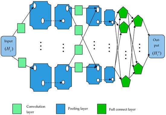
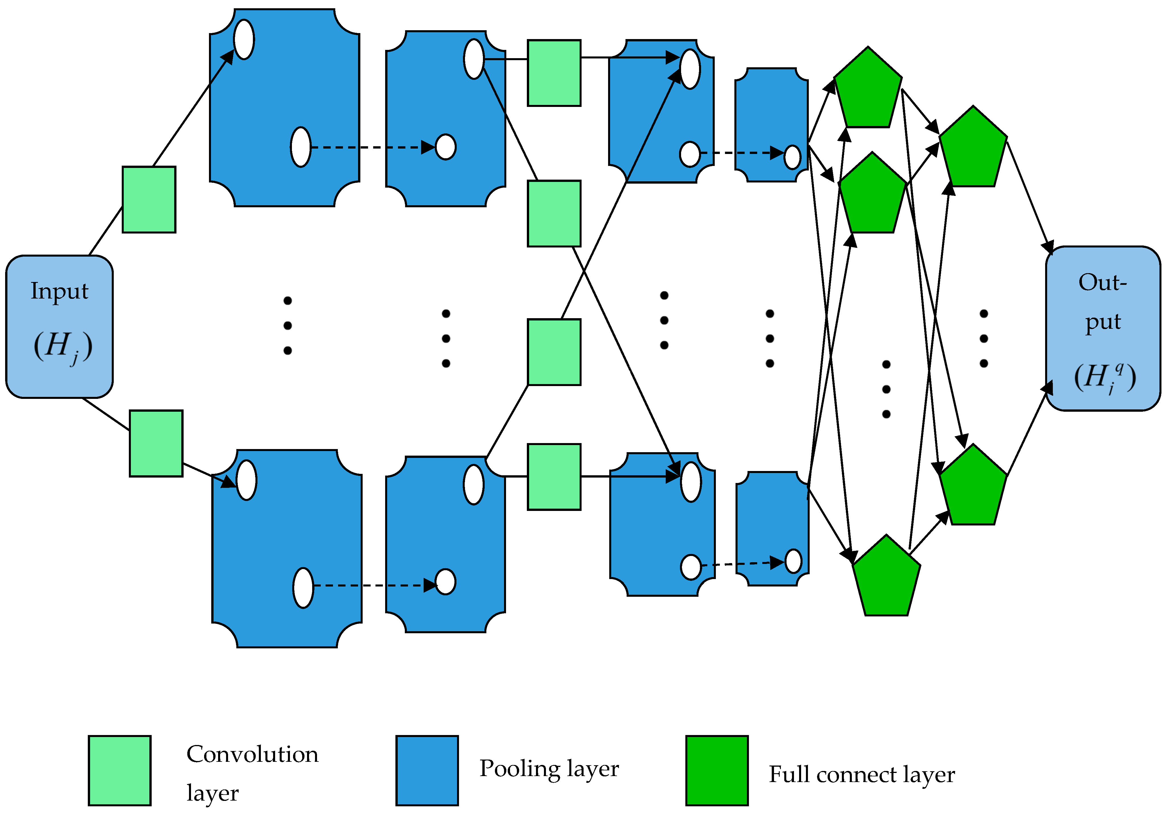
Deep Q Net [22] is a popular deep reinforcement learning method, and the input is considered as. The Deep Q Net employs a Convolutional Neural Network (CNN) for approximating the Q value. The reinforcement learning could be unstable in a few instances. To conquer this instability, Deep Q Net uses the action replay method. Furthermore, expression of the agent’s experience for performing experience replay is formulated as

T_h = (e_h, o_h, f_h, e_h+1)

(8)

B_Q = {T_1,, …, T_h}

(9)

where B_Q is termed as replay memory, and the loss function equation is given below,

$$p_Q({\varphi }_Q)=V\left[ {\left(f+\mathrm{I}\underset{o^{\prime }}{\max } \widehat{\wp }\left(e^{\prime },o^{\prime };{\varphi }_Q^{-}\right)-\wp \left(e,o ; {\varphi }_Q\right)\right)}^2\right]$$

(10)

Here, the discount factor is denoted as, signifies network parameter which is employed for evaluating the target at iteration, and reward is specified as, mentions the network constraint at iteration. To improve the reliability of convergence, DQN acquires a neural fixed Q approach [22]. Moreover, at target is estimated as in a particular period, the output of Deep Q Net is indicated as, and the architecture of Deep Q Net is represented in Figure 2.

Figure 2. Architecture of Deep Q Net.

3.4. Markov Decision Process Formulation for DQN Energy Prediction

To make the DQN formulation reproducible, the WSN energy-prediction task is represented as a Markov Decision Process (MDP). At decision step t, the state s_t contains the normalized residual energy of the relevant sensor nodes/CHs, normalized node coordinates, local node density, the distance-related feature used by the cell-score calculation, and the current fairness-related feature. The state therefore summarizes the network information available at the BS when an energy prediction is requested. The action a_t is a discrete energy-prediction selection: the DQN chooses one of K predefined normalized residual-energy intervals for the candidate cell. The selected interval is mapped to an estimated residual-energy value used by the adjacency-based cell score. The action is therefore an energy-prediction action, not a direct continuous sink-coordinate action.

The reward is defined from the prediction error so that the DQN is encouraged to accurately predict the next observed residual energy. Let E_(t + 1) denote the residual energy observed from the simulator after the transition and Ehat_t denote the energy predicted by the selected action. The reward is defined as r_t = −|E_(t + 1) – Ehat_t|. Consequently, smaller prediction error produces a larger reward. The transition s_t -> s_(t + 1) is generated by the next network state after packet transmission and energy update. The objective is to maximize the discounted return R_t = sum_{k = 0}^{T – t} gamma^k r_(t + k). Experience replay and a periodically updated target network are used as described in Equations (8)–(10). This formulation clarifies that DQN predicts energy, whereas the adjacency-based cell score performs the final mobile-sink placement decision.

Training and inference location: DQN training is assumed to be performed offline at the Base Station (BS) using the simulation/training experience. During network operation, the BS collects the required network-state information, performs DQN inference, evaluates the adjacency-based cell score, and then communicates the selected sink position to the mobile sink. Sensor nodes therefore do not execute the DQN model locally. This design is consistent with the resource constraints of WSN nodes, but it makes the BS a computational dependency.

Deep Q Net successfully predicted the energy of the sink node, based on which the adjacency-based cell score is computed. This optimal location of the mobile sink is identified considering the adjacency-based cell score.

4. Result and Discussion

The outputs of the newly established Deep Q Net are illustrated for predicting the energy during mobile sink placement.

4.1. Experimental Setup

The proposed Deep Q Net-based mobile sink placement is implemented in the Matlab R2024a tool using simulation, and is represented in Table 2. Table 3 presents the DQN architecture and training parameters used to ensure reproducibility of the experiments.

Table 2. Simulation Setup.

Parameter	Values
Number of nodes	100, 200, 300, 400
Number of simulation rounds	2000
Communication radius	50 m
Node initial energy	40 J
Transmit energy	0.6 J
Receiving energy	0.03 J
Network topology	Mesh
Area	250 × 250 m

Table 3. DQN architecture and training parameters for reproducibility.

DQN Parameter	Revised Specification	Purpose
Network input	State vector defined in Section 3.4	WSN energy/context representation
Action space	K discrete normalized residual-energy intervals	Energy prediction
Convolution kernel	3 × 3	Local feature extraction
Convolution filters	32	Feature maps
Stride	1	Convolution step
Pooling window	2 × 2	Dimensionality reduction
Activation	ReLU	Nonlinear mapping
Optimizer	Adam	Network parameter update
Learning rate	0.001	Training step size
Discount factor γ	0.90	Future reward weighting
Replay buffer	10,000 transitions	Experience replay
Mini-batch size	64	Gradient update
Target-network update	Every 100 training updates	Stable Q targets
ε-greedy	εmax = 1.0; εmin = 0.05; linear decay	Exploration/exploitation

4.2. Evaluation Measures

The performance improvement of Deep Q Net-based mobile sink placement is estimated by utilizing evaluation measures, namely energy, normalized throughput, normalized fairness, network lifetime, and distance.

4.2.1. Normalized Throughput

The overall data packets transmitted to the required target through the nodes at a specified time. Moreover, normalized throughput is articulated as

$$ƛ={\displaystyle \frac{\varsigma }{\xi }}$$

(11)

where the overall amount of node counts is symbolized as ς, normalized throughput is specified as ƛ, and time taken by the nodes is characterized as ξ.

4.2.2. Residual Energy

The residual energy existing in nodes after the dissemination of data packets is termed as residual energy. Here, residual energy is modeled as

ħ = 1 − Z_O(F)

(12)

where Z_O(F) represents the consumed energy and residual energy is signified as ħ.

4.2.3. Distance

It is defined as the distance between ${v^{\prime }}^{\mathit{th}}$ and ${q^{\prime }}^{\mathit{th}}$, which is expressed by the equation given below.

$${\omega }_{v^{\prime }{q}^{\prime }}=\left|U_{v^{\prime }}-U_{q^{\prime }}\right|$$

(13)

Here, distance is denoted as ${\omega }_{v^{\prime }{q}^{\prime }}$.

4.2.4. Network Lifetime

This is evaluated by examining the execution of the sensor node, which demonstrates the capability of the method to extend the network lifetime during the transmission of data.

4.2.5. Network Fairness

This is defined as the amount of applications and users fairly using system resources. Moreover, fairness is regularly qualified for resource allocation and sharing in wireless networks.

4.2.6. Mobile-Sink Mobility Cost, Speed, and Collection Latency

The present experimental model evaluates the quality of the selected sink location but does not explicitly simulate the physical movement of the mobile sink. In particular, cumulative travel distance, sink velocity, propulsion/mobility energy, and the latency introduced while moving to and collecting data at the selected location are not included in the five reported evaluation measures. The reported distance metric is therefore a placement-distance measure, not a cumulative mobility-cost measure. The simulation assumes that the mobile sink can reach the selected location within the operational decision interval and that the placement decision is the primary optimization target. This assumption is suitable for studying the placement component, but it does not establish end-to-end deployment feasibility. Accordingly, mobility energy, speed constraints, cumulative trajectory length, and data-collection latency are identified as limitations and should be included in future experiments.

4.3. Comparative Methods

The comparative analysis is executed against the existing methods reported in the original study: DMN [1], Tuft [10], ILP [11], and DMEAAL [12]. Continuous-action reinforcement-learning methods provide an important alternative: DDPG is designed for continuous control [16], PPO is a policy-gradient method [17], and SAC is an off-policy maximum-entropy method for continuous control [23]. The current DQN formulation uses a discrete candidate-cell/energy action space, which is compatible with Q-learning. Directly comparing it with continuous-coordinate methods would require reformulating the action as continuous sink coordinates, and implementing the same state, reward, training budget, and mobility model. Such experiments were not part of the original simulation dataset and are therefore not claimed in the present results. A controlled DQN-versus-DDPG/PPO/SAC study is proposed as future work.

4.4. Comparative Analysis

The comparative analysis of Deep Q Net-based mobile sink placement in relation to performance measures is estimated by varying numbers of rounds for 100 nodes and 200 nodes.

(i)

Analysis based on 100 nodes

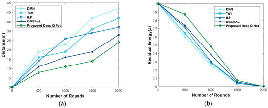
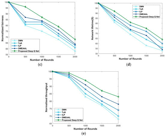
Figure 3 depicts the assessment of Deep Q Net-based mobile sink placement by utilizing various measures based on 100 nodes. In Figure 3a, the valuation of Deep Q Net by varying the number of rounds is illustrated. When the number of rounds is 1000, the distance computed by Deep Q Net is 11 m, and other methods such as DMN, Tuft, ILP and DMEAAL obtained distances of 23 m, 19 m, 26 m, and 16 m. Figure 3b deliberates the analysis of Deep Q Net by varying the number of rounds. Using 500 rounds, the residual energy acquired by DMN is 0.600 J, Tuft is 0.644 J, ILP is 0.712, DMEAAL is 0.738 J and Deep Q Net is 0.874 J. The assessment of Deep Q Net by changing the number of rounds is indicated in Figure 3c. At 1500 rounds, the normalized fairness acquired by DMN, Tuft, ILP, DMEAAL, and the proposed Deep Q Net are 68, 71, 73, 76, and 79. Figure 3d shows the graph between network time and the number of rounds. At 500 rounds, the network lifetime obtained by other models like DMN, Tuft, ILP, and DMEAAL are 81 S, 83 S, 88 S, and 86 S. Moreover, the newly developed Deep Q Net acquired a network lifetime of 92 S. In Figure 3e, the assessment between the number of rounds and normalized throughput is demonstrated. At 2000 rounds, Deep Q Net acquired the normalized throughput of about 83, whereas the other techniques, like DMN, Tuft, ILP, and DMEAAL, obtained the normalized fairness of 68, 70, 74, and 78, respectively.

Figure 3. Valuation regrading 100 nodes for (a) distance, (b) residual energy, (c) normalized fairness, (d) network lifetime, and (e) normalized throughput.

(ii)

Analysis based on 200 nodes

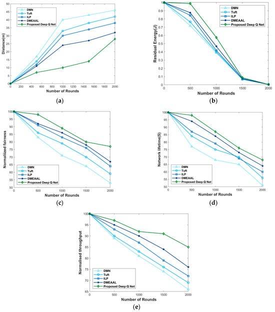
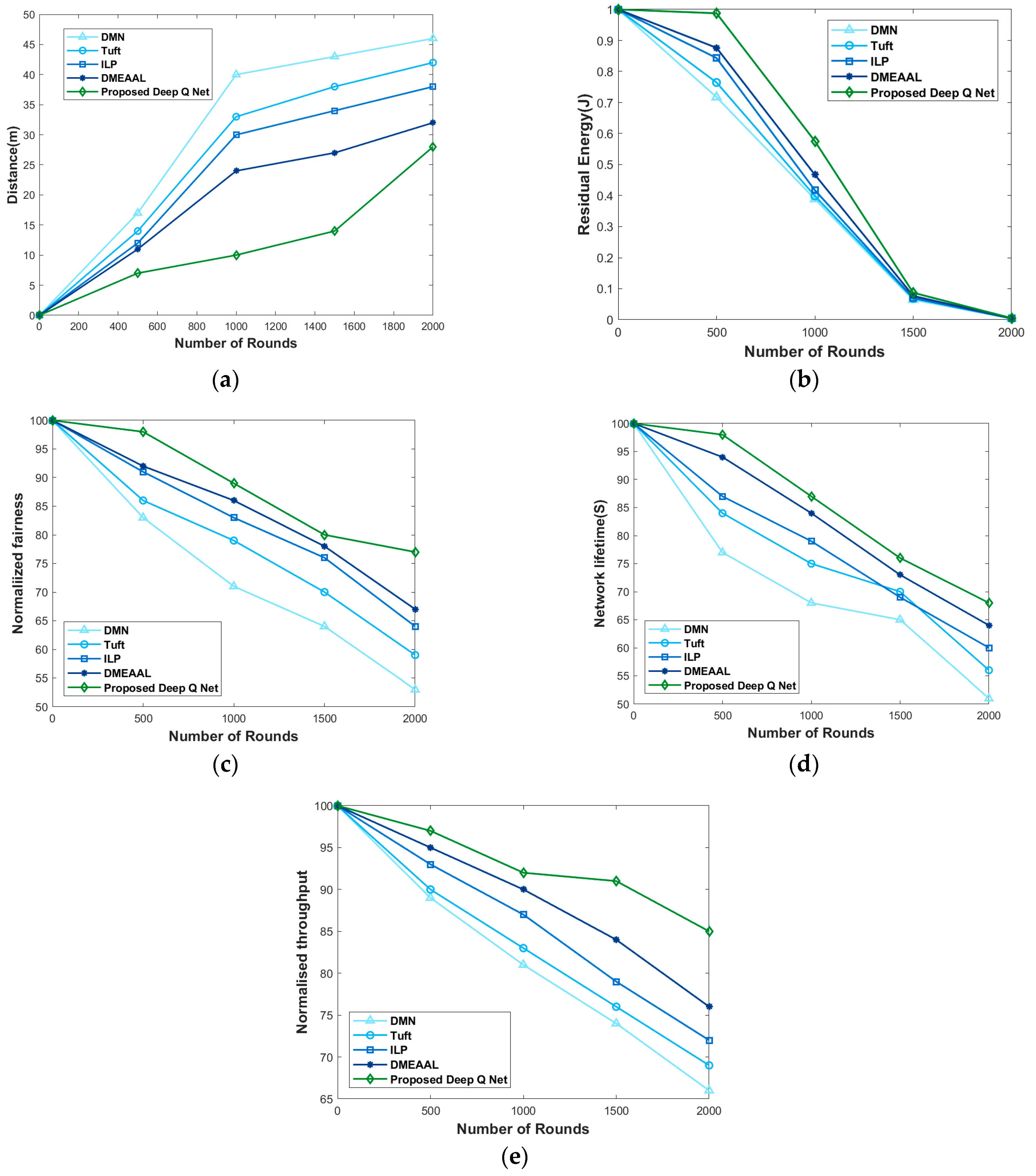
The valuation of Deep Q Net-based mobile sink placement by employing various performance measures based on 200 nodes is portrayed in Figure 4. Figure 4a shows the graph of distance and number of rounds. If the number of rounds is 500, the distance obtained by existing methods like DMN, Tuft, ILP and DMEAAL is 17 m, 14 m, 12 m, and 11 m. Moreover, the newly developed Deep Q Net acquired a distance of 7 m. In Figure 4b, the assessment of Deep Q Net by varying the number of rounds is illustrated. When number of rounds is 1000, the energy obtained by Deep Q Net is 0.576 J, and other methods such as DMN, Tuft, ILP and DMEAAL obtained residual energy of 0.389 J, 0.399 J, 0.418 J, and 0.467 J. In Figure 4c, the graph between the number of rounds and normalized fairness is demonstrated. For 2000 rounds, Deep Q Net attained the normalized fairness of about 77, whereas the other techniques, like DMN, Tuft, ILP, and DMEAAL, obtained the normalized fairness of 53, 59, 64, and 67. The assessment of Deep Q Net is determined by altering the number of rounds, and is indicated in Figure 4d. At 1500 rounds, the network lifetime acquired by DMN, Tuft, ILP, DMEAAL, and the proposed Deep Q Net is 65 S, 70 S, 69 S, 73 S, and 76 S. Figure 4e deliberates the investigation of Deep Q Net by altering the number of rounds. After 500 rounds, the normalized throughput acquired by DMN is 89, Tuft is 90, ILP is 93, DMEAAL is 95, and Deep Q Net is 97.

Figure 4. Valuation concerning 200 nodes for (a) distance, (b) residual energy, (c) normalized fairness, (d) network lifetime, and (e) normalized throughput.

(iii)

Analysis based on 300 nodes

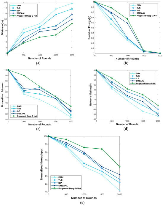
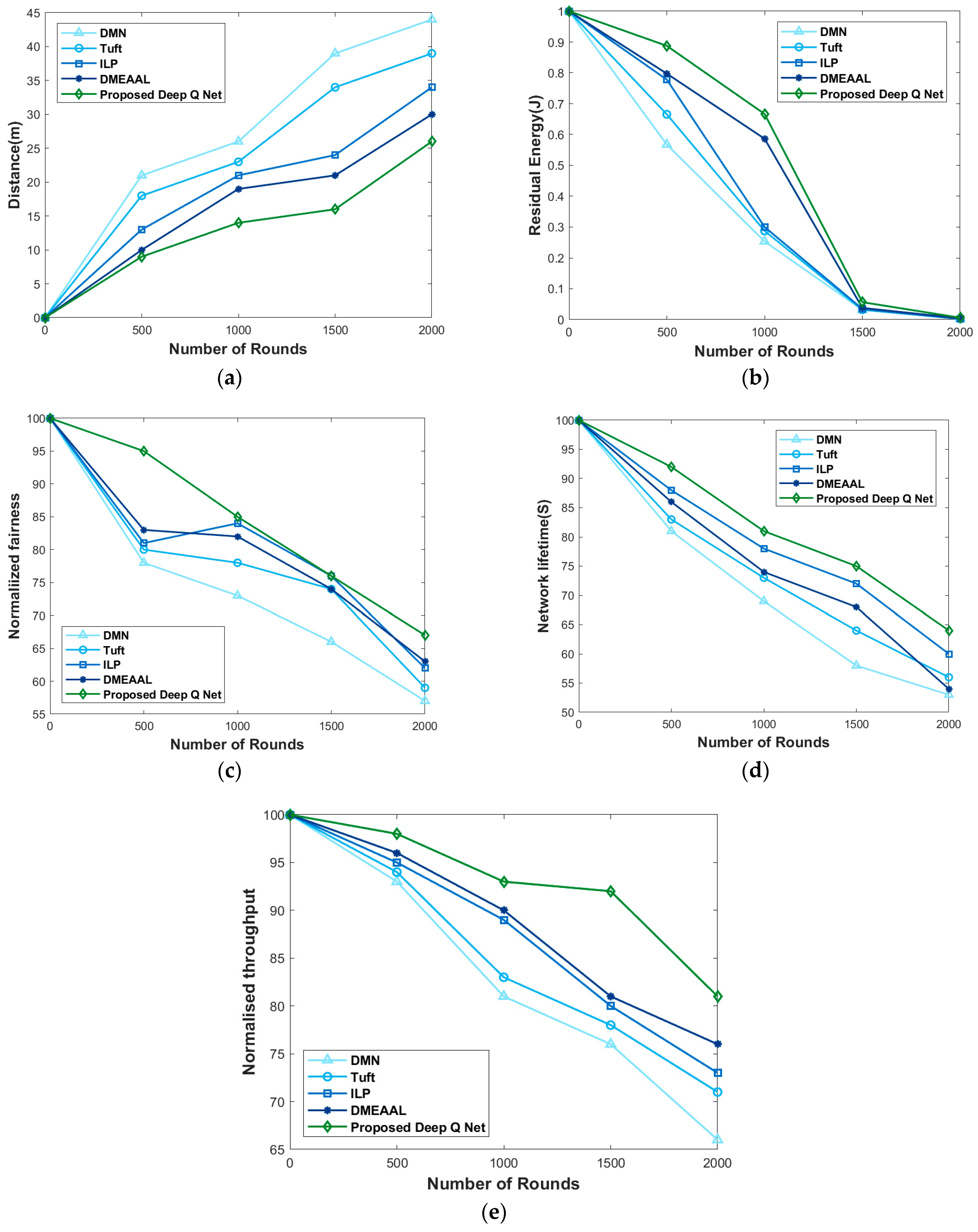
The valuation of Deep Q Net-based mobile sink placement by employing various performance measures based on 300 nodes is delineated in Figure 5. Figure 5a displays the graph between distance and number of rounds. If the number of rounds is 1000, the distance obtained by existing methods like DMN, Tuft, ILP and DMEAAL is 26 m, 23 m, 21 m, and 19 m. Moreover, the newly developed Deep Q Net acquired a distance of 14 m. In Figure 5b, the assessment of Deep Q Net by varying the number of rounds is illustrated. When the number of rounds is 1500, the energy attained by Deep Q Net is 0.056 J, and other methods such as DMN, Tuft, ILP and DMEAAL obtained the residual energy of 0.032 J, 0.032 J, 0.035 J, and 0.038 J. In Figure 5c, the graph between the number of rounds and normalized fairness is demonstrated. For 1000 rounds, Deep Q Net attained the normalized fairness of about 85, whereas the other techniques, like DMN, Tuft, ILP, and DMEAAL, obtained the normalized fairness of 73, 78, 84, and 82. The assessment of Deep Q Net is determined by varying the number of rounds, and is indicated in Figure 5d. At 500 rounds, the network lifetime acquired by DMN, Tuft, ILP, DMEAAL, and Deep Q Net is 81 S, 83 S, 88 S, 86 S, and 92 S. Figure 5e deliberates analysis of Deep Q Net by changing the number of rounds. After 1500 rounds, the normalized throughput acquired by DMN is 76, Tuft is 78, ILP is 80, DMEAAL is 81, and Deep Q Net is 92.

Figure 5. Valuation regrading 300 nodes for (a) distance, (b) residual energy, (c) normalized fairness, (d) network lifetime, and (e) normalized throughput.

(iv)

Analysis based on 400 nodes

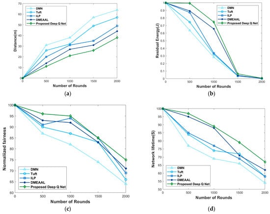
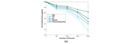
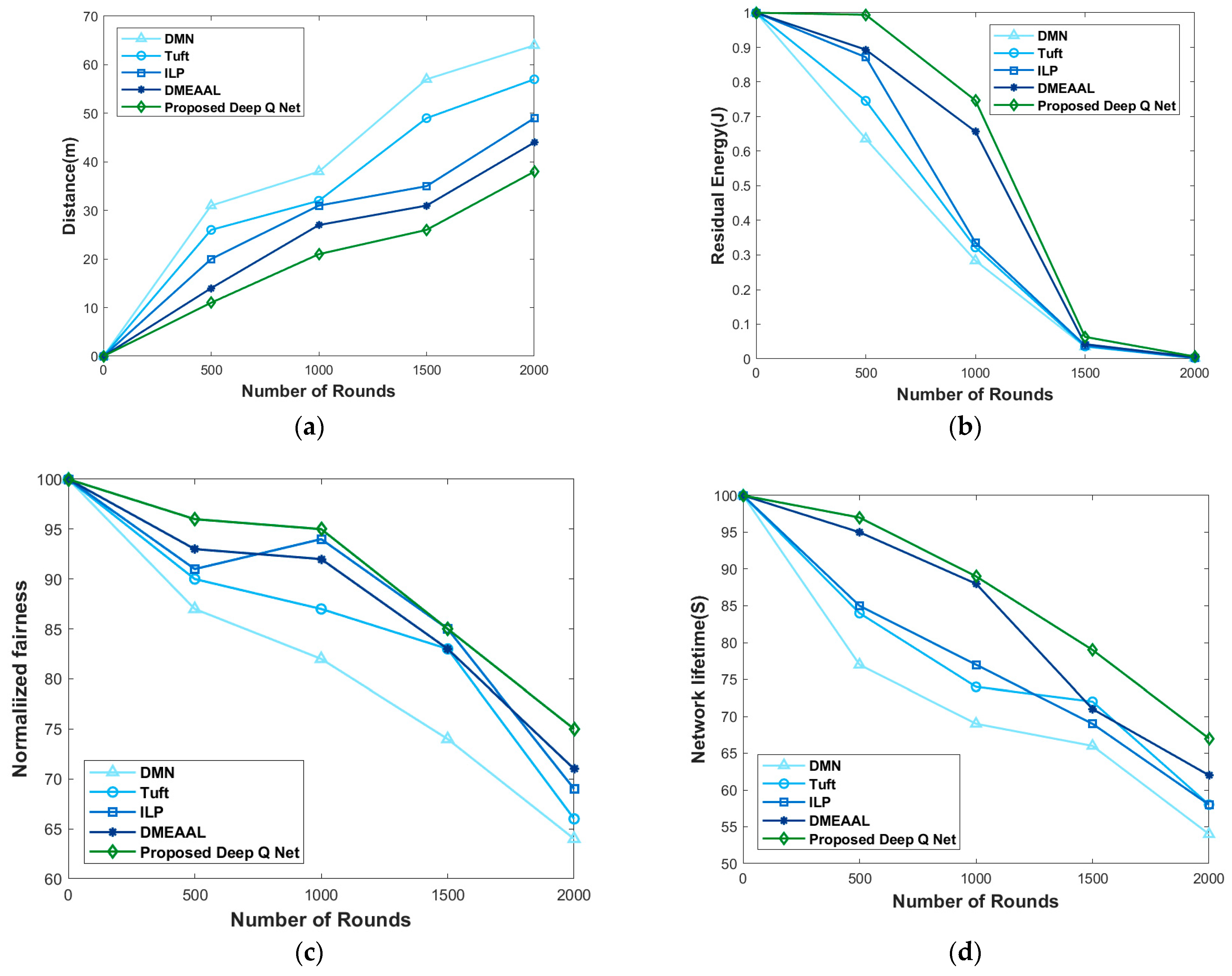
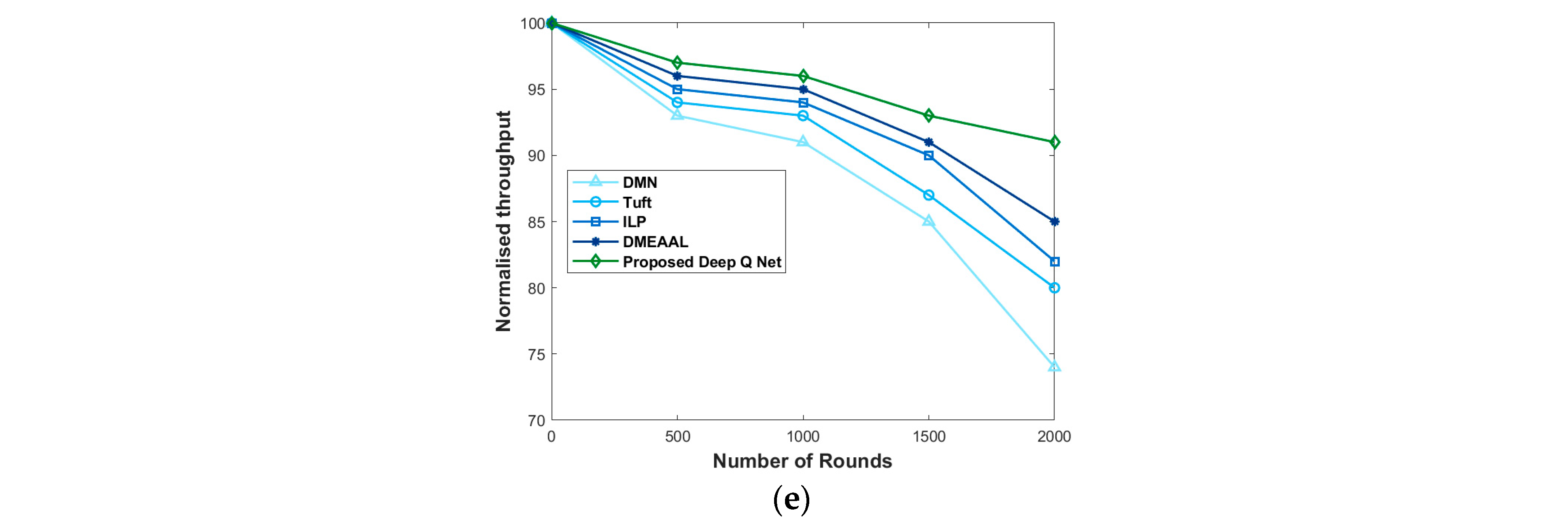
The valuation of Deep Q Net-based mobile sink placement by employing various performance measures based on 400 nodes is delineated in Figure 6. Figure 6a displays the graph between distance and number of rounds. If the number of rounds is 1000, the distance obtained by existing methods like DMN, Tuft, ILP and DMEAAL is 38 m, 32 m, 31 m, and 27 m. Moreover, the newly developed Deep Q Net acquired a distance of 21 m. In Figure 6b, the assessment of Deep Q Net by varying the number of rounds is illustrated. When number of rounds is 1000, the energy attained by Deep Q Net is 0.746 J, and other methods such as DMN, Tuft, ILP and DMEAAL obtained the residual energy of 0.283 J, 0.322 J, 0.322 J, and 0.336 J. In Figure 6c, the graph between the number of rounds and normalized fairness is demonstrated. For 1000 rounds, Deep Q Net attained the normalized fairness of about 95, whereas the other techniques, like DMN, Tuft, ILP, and DMEAAL, obtained the normalized fairness of 82, 87, 94, and 92. The assessment of Deep Q Net is determined by varying the number of rounds and it is indicated in Figure 6d. At 1000 rounds, network lifetime acquired by DMN, Tuft, ILP, DMEAAL, and Deep Q Net is 69 S, 74 S, 77 S, 86 S, and 89 S. Figure 6e deliberates analysis of Deep Q Net by changing the number of rounds. After 1500 rounds, the normalized throughput acquired by DMN is 91, Tuft is 93, ILP is 94, DMEAAL is 95, and Deep Q Net is 96.

Figure 6. Valuation regrading 400 nodes for (a) distance, (b) residual energy, (c) normalized fairness, (d) network lifetime, and (e) normalized throughput.

4.5. Comparative Discussion

The comparative analysis in Table 4 uses the reported values for 100, 200, 300, and 400 nodes. The previous manuscript contained an interpretation error for residual energy in the 300-node case: the proposed method reports 0.006 J, while DMN reports 0.021 J. Because a larger residual-energy value represents more remaining energy, 0.021 J is numerically higher than 0.006 J; the earlier statement that 0.006 J demonstrated an advantage was therefore incorrect and has been removed. The revised discussion reports the values descriptively and avoids that misinterpretation. The abstract and conclusion now use 21 m, which is the smallest distance reported in Table 4 for the 400-node case, rather than the previously repeated 26 m value from the 300-node case.

Table 4. Comparative discussion.

Nodes	Metrics	DMN	Tuft	ILP	DMEAAL	Proposed Deep Q Net
100	Distance (m)	42	37	32	28	24
	Residual energy (J)	0.003	0.003	0.003	0.003	0.004
	Normalized fairness	58	61	63	64	68
	Network lifetime (S)	53	56	60	54	64
	Normalized throughput	68	70	74	78	83
200	Distance (m)	46	42	38	32	28
	Residual energy (J)	0.004	0.004	0.004	0.005	0.005
	Normalized fairness	53	59	64	67	77
	Network lifetime (S)	51	56	60	64	68
	Normalized throughput	66	69	72	76	85
300	Distance (m)	44	39	34	30	26
	Residual energy (J)	0.021	0.002	0.002	0.004	0.006
	Normalized fairness	57	59	62	63	67
	Network lifetime (S)	81	83	88	86	92
	Normalized throughput	66	71	73	76	81
400	Distance (m)	38	32	31	27	21
	Residual energy (J)	0.283	0.322	0.336	0.656	0.746
	Normalized fairness	82	87	94	92	95
	Network lifetime (S)	69	74	77	88	89
	Normalized throughput	91	93	94	95	96

In the proposed method, the network is transformed into various cells using Voronoi partitioning. CH selection is performed using Deep Embedded Clustering (DEC), consistently with Section 3.2 and Algorithm 1. The optimal mobile-sink placement is then obtained from the adjacency-based cell score using predicted residual energy, Euclidean distance, and fairness. The earlier mention of sparse FCM has been removed because FCM is not part of the final proposed method. The reported results should be interpreted as placement-performance results under the stated simulation model.

5. Conclusions

This paper presented a mobile-sink placement framework for WSNs that combines Voronoi partitioning, Deep Embedded Clustering (DEC), an adjacency-based cell score, and Deep Q-Network (DQN)-based residual-energy prediction. DEC is used consistently for CH selection, and the earlier erroneous reference to sparse FCM has been removed. The revised methodology explicitly defines the DQN state, discrete energy-prediction action, reward based on prediction error, and BS-based training/inference arrangement. Based on the reported comparative table, the proposed method records a minimum placement distance of 21 m in the 400-node case, with residual energy of 0.746 J, normalized fairness of 95, network lifetime of 89 s, and normalized throughput of 96 for that reported case. The 300-node residual-energy value of 0.006 J is not interpreted as higher than DMN’s 0.021 J; the numerical values are reported without that previous misinterpretation. The current study focuses on placement optimization and does not quantify mobility energy, speed, cumulative travel distance, or collection latency. These limitations define the scope of the reported results and motivate the proposed future mobility-aware and continuous-action extensions.

6. Limitations and Applicability

The proposed method has several limitations. First, DEC and DQN require more computation than lightweight conventional clustering or heuristic rules. The revised architecture assumes that DQN training and inference are executed at the Base Station, while sensor nodes only provide measurements and receive the final sink decision. This avoids placing the neural-network burden on battery-limited nodes but introduces dependence on BS computation and communication.

Second, the current simulations evaluate 100–400 nodes only. Therefore, performance at networks exceeding 1000 nodes has not been experimentally demonstrated. The principal computational components have different scaling behavior: Voronoi partitioning depends on the number of nodes N, DEC depends approximately on the number of samples, clusters, and optimization iterations, and DQN training depends on the number of replay samples and network parameters. At inference time, the neural-network forward pass is approximately linear in the number of evaluated candidate states, while the overall placement cost also depends on the number of candidate cells and adjacency-score calculations. For large dynamic networks, retraining frequency, BS memory, communication overhead, and candidate-cell reduction become important design factors. Consequently, the current results should not be extrapolated quantitatively to >1000-node deployments without additional experiments.

Third, mobile-sink movement energy, speed limits, cumulative travel distance, and collection latency are not included in the reported results. The method therefore addresses the placement component rather than a complete trajectory-and-collection optimization problem. Fourth, the continuous-action alternatives DDPG, PPO, and SAC have been discussed but not experimentally reproduced in the present dataset.

7. Future Scope

Future work will focus on experimentally validating scalability beyond 400 nodes, including networks with more than 1000 nodes, and on dynamic topologies. A complete mobility-aware formulation should jointly optimize sink position and trajectory while accounting for sink speed, cumulative travel distance, mobility energy, and data-collection latency. Continuous-action reinforcement-learning methods such as DDPG, PPO, and SAC can be evaluated under a common state, reward, training budget, and mobility model. Further work can also investigate multiple mobile sinks, adaptive learning under changing traffic conditions, energy harvesting, security constraints, and real-world testbeds.

References

- Kaur, C.; Hassen, S.M.; Boush, M.S.A.; Anandaram, H. Energy Prediction for Mobile Sink Placement by Deep Maxout Network in WSN. J. Adv. Inf. Technol. 2023, 14, 112–121. [Google Scholar] [CrossRef] [Scilit]
- Poe, W.Y.; Schmitt, J.B. Self-organized sink placement in large-scale wireless sensor networks. In Proceedings of the 2009 IEEE International Symposium on Modeling, Analysis & Simulation of Computer and Telecommunication Systems; IEEE: Piscataway, NJ, USA, 2009; pp. 1–3. [Google Scholar][Green Version]
- Papadimitriou, I.; Georgiadis, L. Maximum lifetime routing to mobile sink in wireless sensor networks. In Proceedings of the SoftCOM 2005, Split, Croatia, 15–17 September 2005. [Google Scholar]
- Poe, W.Y.; Schmitt, J.B. Sink placement without location information in large-scale wireless sensor networks. In Proceedings of the 4th Asian Internet Engineering Conference, Bangkok, Thailand, 18–20 November 2009; pp. 69–76. [Google Scholar]
- Slama, I.; Jouaber, B.; Zeghlache, D. Multiple mobile sinks deployment for energy efficiency in large scale wireless sensor networks. In Proceedings of the e-Business and Telecommunications: International Conference, ICETE 2008, Porto, Portugal, 26–29 July 2008; Revised Selected Papers; Springer: Berlin/Heidelberg, Germany, 2009; pp. 412–427. [Google Scholar]
- Alsalih, W.; Hassanein, H.; Akl, S. Placement of multiple mobile data collectors in wireless sensor networks. Ad Hoc Netw. 2010, 8, 378–390. [Google Scholar] [CrossRef] [Scilit]
- Ar, A.; Chakravarthi, R. Optimal Placement of Mobile Sink in Wireless Sensor Network Using AdjacencyBased Cell Score Factor. Int. J. Intell. Eng. Syst. 2021, 14, 22–32. [Google Scholar] [CrossRef] [Scilit]
- Vijayashree, R.; Dhas, C.S.G. Energy efficient data collection with multiple mobile sink using artificial bee colony algorithm in large-scale WSN. Automatika 2019, 60, 555–563. [Google Scholar] [CrossRef] [Scilit]
- Zhang, L.; Wan, C. Dynamic Path Planning Design for Mobile Sink with Burst Traffic in a Region of WSN. Wirel. Commun. Mob. Comput. 2019, 2019, 1–8. [Google Scholar] [CrossRef] [Scilit]
- Chauhan, V.; Soni, S. Mobile sink-based energy efficient cluster head selection strategy for wireless sensor networks. J. Ambient. Intell. Humaniz. Comput. 2019, 11, 4453–4466. [Google Scholar] [CrossRef] [Scilit]
- Kaswan, A.; Singh, V.; Jana, P.K. A multi-objective and PSO based energy efficient path design for mobile sink in wireless sensor networks. Pervasive Mob. Comput. 2018, 46, 122–136. [Google Scholar] [CrossRef] [Scilit]
- Kumar, D.P.; Tarachand, A.; Chandra, A.; Rao, S. ACO-based mobile sink path determination for wireless sensor networks under non-uniform data constraints. Appl. Soft Comput. 2018, 69, 528–540. [Google Scholar] [CrossRef] [Scilit]
- Sapre, S.; Mini, S. A differential moth flame optimization algorithm for mobile sink trajectory. Peer Peer Netw. Appl. 2020, 14, 44–57. [Google Scholar] [CrossRef] [Scilit]
- Elie, T.; Aline, Z.; Tonye, E. A Reliable and Efficient Path Discovery Method for Mobile Sink based Wireless Sensor Networks. Int. J. Comput. Appl. 2020, 176, 17–22. [Google Scholar] [CrossRef] [Scilit]
- Karpurasundharapondian, P.; Selvi, M. A comprehensive survey on optimization techniques for efficient cluster based routing in WSN. Peer Peer Netw. Appl. 2024, 17, 3080–3093. [Google Scholar] [CrossRef] [Scilit]
- Lillicrap, T.P.; Hunt, J.J.; Pritzel, A.; Heess, N.; Erez, T.; Tassa, Y.; Silver, D.; Wierstra, D. Continuous control with deep reinforcement learning. arXiv 2015, arXiv:1509.02971. [Google Scholar]
- Schulman, J.; Wolski, F.; Dhariwal, P.; Radford, A.; Klimov, O. Proximal Policy Optimization Algorithms. arXiv 2017, arXiv:1707.06347. [Google Scholar]
- Haarnoja, T.; Zhou, A.; Hartikainen, K.; Tucker, G.; Ha, S.; Tan, J.; Kumar, V.; Zhu, H.; Gupta, A.; Abbeel, P.; et al. Soft Actor-Critic Algorithms and Applications. arXiv 2018, arXiv:1812.05905. [Google Scholar]
- Mnih, V.; Kavukcuoglu, K.; Silver, D.; Rusu, A.A.; Veness, J.; Bellemare, M.G.; Graves, A.; Riedmiller, M.; Fidjeland, A.K.; Ostrovski, G.; et al. Human-level control through deep reinforcement learning. Nature 2015, 518, 529–533. [Google Scholar] [CrossRef] [Scilit] [PubMed]
- Sutton, R.S.; Barto, A.G. Reinforcement Learning: An Introduction, 2nd ed.; MIT Press: Cambridge, MA, USA, 2018. [Google Scholar]
- Van Hasselt, H.; Guez, A.; Silver, D. Deep Reinforcement Learning with Double Q-Learning. Proc. AAAI Conf. Artif. Intell. 2016, 30, 2094–2100. [Google Scholar] [CrossRef] [Scilit]
- Mnih, V.; Kavukcuoglu, K.; Silver, D.; Graves, A.; Antonoglou, I.; Wierstra, D.; Riedmiller, M. Playing Atari with Deep Reinforcement Learning. arXiv 2013, arXiv:1312.5602. [Google Scholar] [CrossRef] [Scilit]
- Haarnoja, T.; Zhou, A.; Abbeel, P.; Levine, S. Soft Actor-Critic: Off-Policy Maximum Entropy Deep Reinforcement Learning with a Stochastic Actor. In Proceedings of the ICML 2018, Stockholm, Sweden, 10–15 July 2018; pp. 1861–1870. [Google Scholar]
Disclaimer/Publisher’s Note: The statements, opinions and data contained in all publications are solely those of the individual author(s) and contributor(s) and not of MDPI and/or the editor(s). MDPI and/or the editor(s) disclaim responsibility for any injury to people or property resulting from any ideas, methods, instructions or products referred to in the content. |
© 2026 by the authors. Licensee MDPI, Basel, Switzerland. This article is an open access article distributed under the terms and conditions of the Creative Commons Attribution (CC BY) license.