


Abstract
Continuous health monitoring with wearable sensors frequently suffers from missing data; in geriatric populations device non-compliance, battery depletion, and physiological extremes produce non-random gaps that can distort downstream analysis. Existing methods typically assume a single missingness mechanism and apply a uniform strategy. This study contributes an integrated imputation-and-evaluation framework rather than a new algorithm. The proposed staged method couples k-nearest neighbors (KNN) and support vector regression (SVR), both trained across participants, with a within-participant iterative (MICE-style) refinement that re-estimates each feature conditionally on the others. We evaluate it on window-level features from a public benchmark of 18 older adults (HAR70+) under device-driven failure scenarios spanning MCAR, MAR, and MNAR at three nominal missing-rate settings (10/20/30%), using a leakage-free, leave-one-participant-out protocol with all inference resampled at the participant level, and against mean, KNN, SVR, MICE, missForest, and two temporal baselines. Averaged over 18 conditions and all participants, the staged KNN–SVR–MICE method achieved the lowest reconstruction error (RMSE 0.64, 95% CI [0.61, 0.67]) and the highest explained variance (R2 = 0.62), outperforming every baseline (Holm-adjusted p < 0.001). Linear interpolation was the strongest baseline and the most accurate method under purely random (MCAR) missingness, while the proposed method led under the structured MAR and MNAR scenarios. On a downstream activity-classification task the leading imputers all performed close to the complete-data reference, so the extra reconstruction accuracy did not yield a measurable downstream gain. A real-world ambulatory pilot, reusing pre-existing data, is reported as a feasibility check.
1. Introduction
Continuous health monitoring with wearable sensors suffers significantly from missing data. Missing values can distort the analysis of wearable-sensor data and the conclusions drawn from it [1]. Consequently, hybrid imputation strategies combining statistical and machine-learning techniques provide necessary robustness against these missing values [2,3]. These hybrid methods integrate the predictive strengths of different models. For example, coupling local instance-based methods such as k-nearest neighbors (KNN) with global pattern learners such as support vector machines (whose regression form, support vector regression, SVR, we adopt here), or blending machine-learning algorithms with statistical techniques such as multiple imputation by chained equations (MICE) to leverage complementary strengths and improve accuracy and robustness in estimating missing values [2,4]. Researchers have demonstrated that such combinations can outperform their individual components—for instance, a hybrid of KNN and MICE achieved better imputation accuracy than either method alone in maritime sensor data applications [4]. Similarly, other hybrid frameworks have merged clustering approaches with regression models (e.g., fuzzy c-means clustering combined with SVM-based regression) to exploit both local similarity and global functional relationships, yielding more reliable imputations across diverse scenarios [4].
In the healthcare context, particularly continuous monitoring with wearable sensors, data completeness is very important. Wearable devices used for elderly patient monitoring (e.g., smart bracelets tracking vital signs and activity) often produce datasets with unique patterns of missingness due to device malfunctions, inconsistent patient compliance, and environmental interferences such as connectivity dropouts [5]. Adherence to technology-based exercise programs in older adults varies across interventions [6]. Such missing data are typically not random; instead, they often align with the classical missingness mechanisms defined by Rubin’s taxonomy, missing completely at random (MCAR), missing at random (MAR), and missing not at random (MNAR), each of which poses unique challenges to achieving reliable and accurate data imputation [1]. MCAR refers to data missing for purely random reasons unrelated to any subject or variable attribute (for example, data loss due to an occasional sensor error), whereas MAR describes cases where the probability of missing data depends on the values present in the observed dataset (e.g., patients with certain recorded characteristics are less likely to wear the device) [1]. The most challenging is MNAR, where missingness depends on the unobserved values themselves—for instance, if an elderly patient experiences discomfort (an unrecorded symptom) and consequently removes a health monitor, the missing readings are directly related to that unobserved discomfort. Each mechanism demands different handling: simple approaches may suffice for MCAR data, but biased patterns under MAR or MNAR require more sophisticated techniques to avoid distorted clinical interpretations [1,5].
Existing imputation techniques span a spectrum from basic to advanced. Recent surveys in the Internet of Things (IoT) and healthcare domains highlight a wide array of methods, from statistical imputations and interpolation to machine-learning and deep-learning models, applied to improve data completeness [2,3]. Adhikari et al. [2] provide a comprehensive overview of IoT data imputation strategies, noting that hybrid and ensemble approaches are increasingly popular for their flexibility in various data conditions. In parallel, Liu et al. [3] conducted a methodical review targeting datasets from the healthcare domain, emphasizing the growing effectiveness of advanced imputation methods (including deep neural networks and generative models) across medical data scenarios. However, both studies also underscore that no single method is universally best; performance can vary with the data type, missingness mechanism, and domain requirements [2,3]. Despite extensive imputation efforts in general healthcare and IoT domains, a gap persists in research on wearable sensors in elderly populations. Datasets from geriatric monitoring systems have distinctive characteristics (such as frequent prolonged non-wear periods and correlated missingness with health events) that are not extensively addressed in current studies. Few works have specifically focused on hybrid imputation tailored to these contexts, where mechanism-specific missing data patterns (MCAR vs. MAR vs. MNAR) may demand a contextualized approach for effective recovery of data.
The limitations identified in existing imputation approaches for geriatric health monitoring motivate the development of a new hybrid method explicitly tailored to wearable healthcare data. In recent evaluations [7], we observed that instance-based and margin-based learners (KNN and SVM) consistently outperformed traditional statistical imputations (such as mean, median, or expectation–maximization) and even several advanced models (including Bayesian network imputation, generative adversarial imputation networks, variational autoencoders, and the GRU-D deep-learning model) under scenarios where data were MCAR or MAR. This choice is consistent with independent studies reporting that sophisticated deep-learning imputers do not reliably outperform simpler classical methods when missingness is moderate and the data are limited in size [8,9]. The strength of KNN lies in leveraging local data relationships to fill in gaps based on nearest-neighbor similarities, while SVM (applied either for regression or classification imputation tasks) can capture global patterns via its decision boundaries. However, both methods exhibit limitations under MNAR scenarios: KNN cannot infer missing values when the cause of missingness is tied to information absent from the available feature space, and SVM can become biased when the missingness mechanism alters the underlying data distribution in ways the model is unaware of [10]. These limitations are particularly acute for elderly health datasets under MNAR conditions, where missing data may correlate with critical patient states (e.g., an elderly patient not wearing a heart-rate monitor during episodes of dizziness or pain, precisely when readings would be most medically relevant).
A further limitation of existing work is that most hybrid imputation approaches rarely adapt to the underlying missingness mechanism in a systematic way. Most methods implicitly assume data are at least MAR and apply a one-size-fits-all imputation strategy; few, if any, include a preliminary step to diagnose whether data are MCAR, MAR, or MNAR and then adjust the imputation model accordingly. Recent research demonstrates that analyzing missing-data characteristics can yield insight into the cause of missingness—for example, Braem et al. [5] showed that in wearable sensor data for diabetes patients, the distribution of gap lengths could be analyzed to determine whether missingness followed an MNAR pattern. In addition, the evaluation metrics commonly used in imputation research (RMSE, MAE, R2) may not fully capture real-world clinical utility. Shadbahr et al. [8] argue that imputation quality should also be judged by its impact on downstream machine-learning classifier performance, since the lowest-error method is not useful if it leads to patient misclassification.
Building on these observations, this work develops and evaluates a staged KNN–SVR–MICE imputation method that combines KNN, SVR, and a within-participant MICE refinement, together with a realistic missing-data generation framework grounded in wearable device failure modes. We emphasize that the individual components are well-established techniques, the contribution of this work lies not in a fundamentally new algorithm but in their integration into a staged architecture and, above all, in the systematic and realistic framework within which they are evaluated. The selection of these three components is directly informed by prior empirical findings in which KNN and SVR were the strongest individual machine-learning imputers, complemented by the multivariate, iterative refinement capabilities of MICE. The hypothesis underlying the staged KNN–SVR–MICE method is that combining the predictive strengths of complementary learners—local neighbourhood structure from KNN, global functional structure from SVR, and a final iterative MICE refinement that enforces multivariate consistency—yields more robust performance than any component alone, particularly under the more challenging and realistic missing-data scenarios (including three nominal missingness settings of 10%, 20%, and 30%) investigated here. The ablation in Section 4.6 shows that the decisive factor is the within-participant adaptation rather than the particular combination of learners, and reports transparently where each stage does and does not reduce error. The main contributions of this work are: (1) an integrated imputation-and-evaluation framework that combines established techniques in a staged architecture tailored to wearable geriatric monitoring; (2) a realistic missing-data generation framework that models authentic device-driven failure scenarios across the MCAR, MAR, and MNAR mechanisms, providing a reproducible benchmark; (3) a rigorous validation protocol that separates model training from evaluation and performs all statistical inference at the participant level under a leave-one-participant-out protocol; and (4) a detailed comparative analysis that characterizes the behaviour of the methods across mechanisms, missing rates, and sensor types, including the conditions under which the staged KNN–SVR–MICE method is and is not advantageous.
2. Related Work
2.1. Missing Data in Health Monitoring Systems
Continuous health monitoring is essential for detecting conditions like frailty and depression in older adults, but its clinical utility is severely limited by missing data. In ambulatory settings, device malfunctions, user non-compliance, and environmental interference frequently interrupt data collection. In our previous work on the Frailty Insights Detection System (FIDS) [11], incomplete data emerged as a primary bottleneck compromising system reliability. Consequently, resolving these data gaps is a strict prerequisite for accurate frailty detection.
Missing-data mechanisms follow the three categories of Rubin’s taxonomy introduced above (MCAR, MAR, MNAR) [1,12], of which MNAR is the most challenging and most likely to induce clinical bias if handled naively.
2.2. Advancements in Missing Data Imputation
Many machine-learning models require complete inputs, so managing incomplete data in dynamic IoT and healthcare environments remains a persistent challenge, and the literature shows a clear transition from basic statistical imputation to machine-learning and deep-learning approaches [2,3,13]. Hybrid and ensemble models [14] and Bayesian techniques [15] handle complex missing-data patterns well; however, while deep generative models such as GAIN and VAE excel on massive datasets [3,9], classical machine-learning and time-series methods often give more reliable real-time imputation for specific hardware deployments such as marine or wearable sensor networks [16].
The appropriate strategy depends on the mechanism: listwise deletion or mean imputation can suffice under MCAR but underestimate variance [17], whereas MAR and especially MNAR require multivariate or specialized techniques (e.g., KNN, MICE, autoencoders, or pattern-mixture models) to preserve relationships and correct mechanism-induced bias [18].
Beyond reconstruction accuracy, the downstream impact of imputation has received increasing attention. Shadbahr et al. [8] emphasize the importance of imputation quality when developing machine-learning classifiers on datasets with missing values, showing that both the chosen imputation approach and the degree of data absence significantly affect classifier performance. By analyzing datasets with simulated and real-world missingness, they investigated how methods such as mean imputation, missForest, MICE, GAIN, and the missing-data importance-weighted autoencoder (MIWAE) affect not only reconstruction accuracy but also the interpretability of classification models, underscoring the need for robust evaluation criteria beyond error metrics alone.
Our comparison deliberately focuses on robust classical and ensemble imputers (mean, KNN, SVR, MICE, missForest) rather than deep generative models such as GAIN, VAE, or GRU-D. This choice is motivated by the low-data regime: the dataset comprises a few thousand records from a small number of participants, a setting in which deep imputers are typically data-hungry and prone to overfitting, and in which prior comparative evidence, including our own earlier evaluation [7], indicates that they do not reliably outperform simpler methods. The objective here is therefore to identify the most robust and reproducible imputation strategy for low-data wearable settings; benchmarking deep generative imputers on substantially larger geriatric datasets is left to future work.
3. Materials and Methods
3.1. Datasets
This study evaluates the proposed framework on two complementary datasets, addressing the problem on two fronts: a recognized public benchmark that supports transparency and reproducibility, and a pre-existing real-world pilot that illustrates applicability under uncontrolled ambulatory monitoring. Their principal characteristics are compared side by side in Table 1.
Table 1.
Side-by-side comparison of the two datasets used in this study: the public HAR70+ benchmark (Dataset A, primary methodological validation) and the proprietary real-world pilot (Dataset B). Full collection details for Dataset B are reported in [7].
Dataset A—HAR70+ (primary methodological validation). HAR70+ is a public dataset of wearable accelerometer recordings from 18 older adults aged 70–95 years [19]. We adopt it as our primary validation dataset precisely because, as an openly available and widely used benchmark from a geriatric population, it supports transparency and reproducibility. The raw 50 Hz back- and thigh-mounted accelerometer signals were segmented into non-overlapping 3 s windows, from which 19 numeric features were extracted (per-axis means and standard deviations, signal magnitudes, and cross-axis correlations), yielding 13,571 labelled windows across the four activity classes retained for this study (walking, sitting, standing, lying); the remaining HAR70+ activities (shuffling, stair ascending, stair descending) are not included in this subset.
Dataset B—real-world ambulatory pilot. To demonstrate the applicability of the framework under the uncontrolled conditions of real-world ambulatory monitoring, we additionally evaluate it on a proprietary dataset obtained from our own hardware implementation. This pilot comprises 3845 multivariate measurements collected from wrist-worn devices integrating accelerometer, gyroscope, orientation, and heart-rate sensors, sampled at approximately 10–50 Hz over several days. The data collection protocol and sensor placement follow the methodology established in our previous work [20]. It was recorded by the authors (adult, non-geriatric participants) rather than from an elderly cohort; it therefore serves as a feasibility check that the method behaves sensibly on genuinely collected multi-sensor data under live conditions, complementing—but not substituting for—the geriatric benchmark validation on Dataset A.
3.2. Realistic Missing Data Generation
To effectively evaluate a hybrid imputation method, missing-data patterns are required that approximate real-world scenarios in wearable sensor applications. Traditional approaches to generating missing data for method evaluation often rely on simplistic random removal of values, which fails to capture the complex patterns observed in actual wearable device usage, particularly among elderly populations. To address this limitation, we developed a framework for generating missing-data patterns in wearable sensor datasets motivated by documented device failure modes and usage patterns. The framework consists of three main components: (1) automatic identification of sensor groups from the column structure of the input dataset, independent of any fixed sensor schema; (2) implementation of six distinct scenarios realizing the three missing-data mechanisms (MCAR, MAR, MNAR) defined in Rubin’s taxonomy [1]; and (3) configurable missing-data percentages and scenario-specific parameters. The framework takes as input a complete dataset (without missing values) and produces multiple datasets with missing values introduced according to the specified scenarios and percentages. Because the grouping step is driven by each dataset’s own columns rather than a predefined sensor list, the framework applies without modification to wearable datasets with heterogeneous sensor configurations, as demonstrated on the two datasets used in this study (Section 4), which differ substantially in their sensor composition.
3.2.1. Sensor Group Identification
Wearable devices vary widely in their sensor configurations, and any realistic missing-data framework must accommodate datasets whose available signals differ. Rather than assuming a fixed set of sensors, the framework infers sensor groups from the column structure of each input dataset, assigning columns to functional groups according to the signal type they represent (e.g., accelerometric channels, derived magnitude or correlation features, and activity or temporal metadata). The specific groups that emerge therefore depend on the dataset. In the primary HAR70+ dataset, this procedure yields groups corresponding to the back- and thigh-mounted triaxial accelerometers (e.g., back_x, back_y, back_z, thigh_x, thigh_y, thigh_z), together with derived statistical features and an activity label. In the real-world pilot dataset (Section 4.7), which provides a richer sensor suite, the same procedure additionally identifies gyroscope, orientation, and heart-rate groups. This data-driven grouping is used to implement the failure scenarios. We note an important caveat about its physical interpretation: the groups are defined from the column structure, so statistics derived from the same raw signal (for example, a per-axis mean, the corresponding magnitude, and a cross-axis correlation) are treated as separate groups and can be masked independently. A true physical sensor failure would remove all features derived from that sensor together, whereas our masks may remove an axis statistic while retaining a magnitude computed from the same axis. The six scenarios should therefore be read as reproducible, feature-level stress tests that emulate the statistical structure of device-driven gaps (duration, burst, activity- and value-dependence), rather than as exact physical simulations of hardware failure. This does not affect the imputation task or the ground truth, which are defined at the feature level; it qualifies only the device-level interpretation of the scenarios.
3.2.2. Realistic Missing Data Scenarios
Six distinct scenarios were implemented across the three missing-data mechanisms, each modelling a specific real-world situation encountered in wearable sensor applications. Figure 1 provides an overview of the six scenarios, grouped by mechanism, with a schematic of the characteristic missing-data pattern each one produces.
Figure 1.
Overview of the six realistic missing-data scenarios, grouped by the three mechanisms of Rubin’s taxonomy (MCAR, MAR, MNAR). In each grid, rows correspond to sensor groups and columns to time; grey cells denote observed values and coloured cells denote missing values, illustrating the characteristic gap pattern of each scenario.
The six scenarios are defined as follows:
MCAR—Scenario 1 (Random Sensor Failures): individual sensors randomly fail for short periods, representing hardware failures occurring independently of other factors. A random sensor group is selected, a random failure duration is determined (e.g., 5–20 consecutive measurements), a random starting point is chosen, and all measurements from the selected group are set to missing for the failure duration.
MCAR—Scenario 2 (Temporary Connection Issues): all sensors fail simultaneously for short periods, simulating Bluetooth or wireless connection problems. A random connection-issue duration (e.g., 3–15 consecutive measurements) and starting point are chosen, and all sensor measurements are set to missing for that duration.
MAR—Scenario 3 (Activity-Dependent Sensor Failures): certain sensors are more likely to fail during specific activities (e.g., accelerometer readings missing more often during high-intensity activities). Sensor–activity relationships are defined and a higher probability of missingness is applied to the associated sensors for each activity.
MAR—Scenario 4 (Battery Depletion Patterns): sensors gradually fail as the battery depletes, with different sensors failing in a specific order based on power requirements (e.g., the most power-hungry sensor first, low-power accelerometers last). Failure points are computed along the time dimension, and values are set to missing from each sensor’s failure point onward; this is a time- and usage-dependent, MAR-style pattern.
MNAR—Scenario 5 (Value-Dependent Sensor Failures): sensors are more likely to fail when producing extreme values. For each sensor, extreme values are identified (e.g., top 20% of absolute values) and a proportion of these are set to missing, reflecting sensor saturation or measurement difficulty at extremes—particularly relevant for fall detection.
MNAR—Scenario 6 (Sensor Range Limitations): sensors fail to record values outside their operating range (e.g., an accelerometer saturating beyond its full-scale acceleration limit). Upper and lower limits are defined based on percentiles of the observed distribution, and values outside these limits are set to missing.
Scenarios 5 and 6 are described as MNAR-like rather than strictly MNAR: the missingness is driven by the value that would have been observed, which is the defining feature of MNAR, but it is induced synthetically so that ground truth is available for evaluation. True MNAR in deployed systems cannot be verified without the unobserved values themselves; these scenarios therefore approximate, rather than fully reproduce, real MNAR mechanisms, and are intended to stress-test imputation under value-dependent missingness.
The six scenarios are controlled by explicit, reproducible parameters. The generator uses three nominal intensity settings, r ∈ {0.10, 0.20, 0.30}; the realized proportion of masked cells depends on the scenario and is reported separately (below and in the released per-participant data). Random sensor failures use a failure duration drawn uniformly from 5–20 consecutive measurements applied to a randomly selected sensor group; temporary connection issues use a duration of 3–15 consecutive measurements applied to all sensors. Activity-dependent failures apply, to each sensor associated with the current activity, a per-measurement missingness probability of min(0.5, 3 × rate). Battery depletion fails sensors in a fixed power-order, setting each sensor missing from a failure point onward so that earlier-failing sensors lose more measurements; the number of affected rows is set from the intensity parameter (for this scenario it realizes roughly half the nominal value). Value-dependent failures mark the top 20% of each channel’s absolute values (above the 80th percentile) as candidate extremes and set each to missing with probability min(0.8, 3 × rate × extremeness), where extremeness scales from 0 at the threshold to 1 at the channel maximum. Range limitations drop values below the (rate/2) quantile or above the (1 − rate/2) quantile of each channel. Runs use fixed random seeds (reported in the released code). Importantly, the rate is a per-scenario intensity parameter rather than a guaranteed global missing fraction: the two MCAR scenarios and the MNAR range-limitation scenario realize close to the nominal 10/20/30%, whereas the activity-dependent (realized ≈8/14/14%), battery-depletion (≈5/11/16%) and value-dependent (≈2/4/5%) scenarios realize lower fractions because their rules are bounded—value-dependent failures, for example, draw only from the top 20% of extreme values and so cannot reach 30%. Averaged over all scenarios, the three settings correspond to overall realized fractions of about 8%, 15%, and 21%; the realized per-participant fractions for every scenario and rate are reported in the released data. The implementation is provided as a Python class that can be applied to any wearable sensor dataset.
3.3. Hybrid Imputation Method
The proposed method combines statistical preprocessing and machine-learning-based predictive modelling in a staged, iterative workflow. As illustrated in Figure 2, it consists of three stages applied after preprocessing: a training phase on complete data, in which the per-feature SVR models are fitted; an iterative KNN–SVR imputation phase, in which local and global estimates are combined to fill the missing values; and a final within-participant MICE-style refinement that, starting from the KNN–SVR estimate, re-estimates each missing entry by chained conditional regression on the other features. This staged design lets the method leverage the complementary strengths of local (instance-based), global (model-based) and iterative multivariate imputation while mitigating their individual weaknesses. The initial steps involve data acquisition from wearable devices and preprocessing, including removal or correction of erroneous data points, standardization and normalization of data formats, and identification of missing values and their patterns (which may follow MCAR, MAR, or MNAR).
Figure 2.
Architecture of the staged KNN–SVR–MICE method: a training phase that fits the scaler and the per-feature SVR models on complete data, and an iterative imputation phase that combines a local KNN estimate with the global SVR estimate (0.6·SVR + 0.4·KNN) over five cycles. A final MICE refinement stage then initializes from the KNN–SVR estimate and applies chained within-participant Bayesian ridge regressions over several cycles to enforce multivariate consistency; it is part of the final method, and its contribution is quantified in Section 4.6.
3.3.1. Training Phase on Complete Data
Before addressing missingness, a training phase is executed on a fully observed dataset. A complete subset without gaps is selected to ensure the models learn from reliable information. The data are transformed using a standard scaler so that every feature has a mean of 0 and a standard deviation of 1 (Equation (1)), a step essential for algorithms sensitive to data scales, such as SVR and KNN:
where X is the original data, μ is the feature mean, and σ is the feature standard deviation. Two complementary models are then trained on the complete data. Support vector regression (SVR), using a radial basis function (RBF) kernel, is trained to predict each variable from all other variables, capturing non-linear relationships (Equation (2)):
where K(xi, x) is the kernel function, αi and αi* are dual coefficients, and b is the bias term. Simultaneously, a k-nearest neighbors imputer is prepared to handle local data patterns using uniform weighting over the k-nearest neighbors. At the end of this phase, both models are optimized for subsequent imputation. The SVR component is the most computationally intensive part of the training phase, requiring explicit training on the complete data to learn the non-linear relationships between variables, whereas KNN training is implicit and occurs during the imputation phase. The SVR hyper-parameters (RBF kernel, C = 100, ε = 0.1, γ = scale) were fixed a priori rather than tuned on the evaluation data, to avoid any optimistic bias: a relatively high regularization parameter C = 100 was chosen because the standardized sensor features are smooth and low-noise, so a tighter fit is beneficial, while ε = 0.1 keeps a modest insensitivity tube; the KNN neighbourhood (k = 5, Manhattan distance, uniform weights) follows common practice for this feature dimensionality. We confirmed in a sensitivity check that moderate changes to these values (C in {10, 100}, k in {5, 10}) did not alter the method ranking.
z = (X − μ)/σ,
f(x) = Σ (αi − αi*) K(xi, x) + b,
3.3.2. Iterative Hybrid Imputation Phase
After training, the system applies iterative imputation to datasets containing missing values. The incomplete dataset is first standardized using the scaler parameters previously fitted on the complete data, ensuring alignment between phases. The KNN imputer then provides preliminary estimates by filling missing values based on the closest neighbouring observations in the standardized feature space—a step particularly effective for MCAR and MAR patterns, as it leverages local similarity structures. Using the KNN-imputed dataset, the trained SVR models predict the missing values based on non-linear relationships between features, capturing complex dependencies not evident in the local neighbourhood structure. At each masked entry the KNN and SVR estimates are combined by a fixed convex blend favouring the global SVR estimate, 0.6·SVR + 0.4·KNN; this weighting was set a priori—reflecting that once a reliable local initialization exists the global model carries most of the corrective information—and a sensitivity check over blends from 0.5 to 0.7 left the method ranking unchanged. Observed entries are held fixed, and the combined estimates are rescaled to the original space by inverse transformation (Equation (3)):
X_original = z · σ + μ,
This KNN–SVR update cycle is repeated five times, which in our experiments was sufficient for the masked estimates to stabilize—changes between successive cycles fell below 1% of the signal range—while additional cycles did not improve accuracy. The complete procedure is summarized in Algorithm 1.
| Algorithm 1. Staged KNN–SVR–MICE imputation (training and imputation) |
| Input: complete training matrix X_train (17 participants); evaluation matrix X_eval with missing mask M; k = 5; C = 100; ε = 0.1; blend w = 0.6; cycles T = 5. Training phase (on X_train only): 1. Fit scaler S on X_train; X_train ← S(X_train). 2. For each feature j: fit SVR_j (RBF, C, ε) to predict column j from the other columns of X_train. Imputation phase (on X_eval): 3. X ← S(X_eval); keep observed entries fixed, masked entries set to NaN. 4. Repeat T times: a. KNN step: for each masked entry (i,j), estimate v_KNN from the k nearest rows (Manhattan) using the other, mean-filled columns. b. SVR step: for each masked entry (i,j), predict v_SVR = SVR_j(other columns of row i), where any still-missing predictor cells are filled with the current KNN estimate (column means on the first cycle), so the SVR never receives NaN inputs. c. Blend: X[i,j] ← w·v_SVR + (1−w)·v_KNN; restore observed entries. 5. MICE refinement: initialize from the KNN–SVR output X; for a fixed number of cycles, update each feature’s missing cells with a Bayesian ridge regression fitted on the held-out participant’s own observed windows, using the current estimates of the other features as predictors. 6. Return S−1(X) (inverse-scaled, fully imputed evaluation matrix). |
3.3.3. MICE Refinement Stage
The third stage is a MICE refinement applied to the output of the KNN–SVR stage. We distinguish two MICE settings used in this paper to avoid ambiguity. The standalone “MICE” baseline (Section 4) is a standard IterativeImputer with a BayesianRidge estimator fitted on the training participants and applied directly to the masked evaluation matrix. The refinement stage inside the proposed method is different and operates within the held-out participant: it is initialized with the KNN–SVR estimate and then applies chained conditional regressions (BayesianRidge), updating each feature’s missing cells in turn from that participant’s own observed windows while using the current estimates of the other features as predictors, for a fixed number of cycles. Because the KNN–SVR output provides both the initialization and the context for the first pass, the refinement improves on it rather than replacing it: the ablation in Section 4.6 shows that starting the refinement from the KNN–SVR estimate yields a lower error than starting it from a mean fill, so the cross-participant KNN and SVR stages genuinely contribute to the final within-participant refinement. MICE applies a series of chained regression equations iteratively to correct residual biases and ensure multivariate consistency, estimating missing entries in each feature from the other variables and improving these estimates over iterations (Equation (4)):
where Xj is the feature being imputed, X−j(t) represents all other features at iteration t, and θ represents the parameters of the conditional model. The refinement improves multivariate consistency and partially mitigates structured bias in MNAR-like scenarios, although it does not explicitly model the MNAR mechanism; rigorous MNAR handling would require selection or pattern-mixture models that are outside the scope of this work. The ablation in Section 4.6 reports its contribution under a matched comparison; it is retained as the final stage of the proposed pipeline.
Xj(t+1) = f(X−j(t), θ),
3.4. Experimental Setup and Evaluation
The proposed KNN–SVR–MICE method was evaluated against eight alternatives—mean imputation, KNN, SVR, standard MICE, missForest, two temporal baselines (last-observation-carried-forward, LOCF, and linear interpolation along the window sequence), and its own two-stage KNN–SVR ablation—across all six realistic scenarios at three nominal missingness settings (10%, 20%, 30%), yielding 18 test conditions (6 scenarios × 3 nominal settings), evaluated under the leave-one-participant-out protocol described in Section 3.5. All methods were implemented in Python 3.10 using scikit-learn 1.2.2 (KNN, SVR, IterativeImputer/MICE, missForest via IterativeImputer with a RandomForestRegressor, and the downstream RandomForestClassifier), pandas 2.0.0 and numpy 1.24.3 (data manipulation), and matplotlib 3.7.1 (visualization). All experiments were carried out on a system with an Intel Core i7-11800H processor (Intel, Santa Clara, CA, USA) and 32 GB RAM, running Ubuntu 22.04. The key hyper-parameters of all methods are listed in Table 2 to support reproducibility; the complete code, scenario generator, and configuration are publicly available (see the Data Availability Statement).
Table 2.
Key hyper-parameters of all imputation methods and of the downstream classifier, for reproducibility.
The full factorial design crossing the six scenarios with the three missing rates is summarized in Figure 3.
Figure 3.
Factorial experimental design. The six missing-data scenarios (rows, grouped by mechanism) are crossed with three nominal missingness settings (columns: 10%, 20%, 30%), yielding 18 test conditions, each evaluated for all nine imputation methods compared in this study.
Imputation quality was assessed using root mean square error (RMSE), mean absolute error (MAE), normalized RMSE (NRMSE, RMSE normalized by the range of actual values to allow comparison across variables), and the coefficient of determination (R2). In addition, the preservation of statistical properties of the original data was evaluated, including mean and standard deviation, the correlation structure between variables, and distribution characteristics (skewness and kurtosis). Statistical significance of performance differences was assessed using two-sided paired permutation tests at the participant level, with Holm correction across the family of comparisons and Cohen’s d_z as an effect-size measure.
3.5. Experimental Validation Protocol
To ensure that the reported results reflect genuine imputation performance rather than either row-level or participant-level information leakage, the evaluation used a strict leave-one-participant-out (LOPO) protocol. Because HAR70+ contains only 18 participants, splitting at the window level would place windows from the same person in both the training and the evaluation sets; the near-duplication between a participant’s own windows would then make imputation appear artificially accurate. We therefore treat the participant as the unit of splitting. In each of the 18 folds, one participant is held out entirely as the evaluation set and the remaining 17 form the complete, fully observed training (donor) set. The cross-participant components—the scaler, the KNN donor pool, and the per-feature SVR models—are fitted using only these 17 training participants, so no window from an evaluated participant is seen when they are fitted. The final MICE refinement, by contrast, adapts to the held-out participant using only that participant’s observed entries; the masked ground-truth values are excluded from all fitting and updates. Because the refinement uses all of the held-out participant’s observed windows, including those following a gap, the pipeline is evaluated as an offline imputation procedure (as is linear interpolation, which can likewise use later observations); real-time use would require a causal variant and is out of scope here. Within each fold, and for each of the 18 conditions (6 scenarios × 3 missing rates), missing values are introduced only into the held-out participant’s windows using the realistic generator; the original values at the masked positions are retained as ground truth and never exposed to any model.
All methods receive exactly the same information. A single StandardScaler is fitted on the 17-participant training set and applied to both training and evaluation windows, so reconstruction error is measured in standardized (z-score) units that are comparable across the heterogeneous sensor channels. Every model-based method—KNN (whose donor pool is the standardized training set), SVR, MICE, missForest, the two-stage KNN–SVR method, and the cross-participant stages of the KNN–SVR–MICE variant—are fitted on this same clean training set, while its MICE refinement operates entirely within the held-out participant, re-estimating that participant’s missing cells from its own observed windows and using no information from the masked ground truth; the mean baseline uses training-set column means. This removes any inequality in the information available to the different methods. For the ablation (Section 4.6), the KNN component is implemented identically across all variants–fitted on the held-out participant’s own observed windows–so that adding or removing the SVR or refinement stage is the only change between variants and the comparison is matched. The activity label is used only for the downstream classifier (Section 4.5) and is excluded from the imputation feature matrix and from every derived feature throughout.
Each condition is thus evaluated once per held-out participant, giving 18 independent participant-level observations per method and condition. Because these observations are the natural independent unit, all inference in Section 4 is performed at the participant level: point estimates are means over the 18 participants. Furthermore, 95% confidence intervals are obtained by a cluster bootstrap that resamples the 18 participants (5000 resamples). Pairwise comparisons use the participant-level mean difference, with p-values from a two-sided paired sign-flip permutation test (20,000 permutations); the Holm correction is then applied to these p-values across the family of eight comparisons. Cohen’s d_z is reported as an effect size and is not itself corrected. This participant-level treatment, rather than pooling scenario × rate × seed observations that share the same 18 people, is what keeps the reported uncertainty well-calibrated.
4. Results
4.1. Overall Performance
Table 3 reports the overall performance of all nine methods on the HAR70+ benchmark under the leave-one-participant-out protocol as the mean over all 18 participants and all 18 conditions, reported as the participant-level mean ± standard deviation across participants; the 95% confidence interval for the headline method is obtained separately from the participant-level cluster bootstrap. Reconstruction error is expressed in standardized (z-score) units. The staged KNN–SVR–MICE method achieved the lowest reconstruction error (RMSE 0.637, 95% CI [0.605, 0.670]) and the highest explained variance (R2 = 0.622), ahead of its two-stage KNN–SVR ablation (0.747) and of every other method, including the two temporal baselines—linear interpolation along the window sequence (0.694), the strongest of the baselines in Table 3, and LOCF (0.781)—as well as missForest (0.952), KNN (0.968), standard MICE (0.987), mean imputation (1.222), and SVR (1.330). The gap to the strongest competitor, linear interpolation, is a mean participant-level difference of −0.058 in RMSE (95% CI [−0.085, −0.032], Holm-adjusted p < 0.001, Cohen’s d_z = 0.96); the gap to the two-stage ablation is −0.110 (95% CI [−0.160, −0.069], p < 0.001); the paired comparisons against every method are reported in Table 4. Notably, SVR alone performed worst overall, below even mean imputation, because the per-feature SVR models, fitted across heterogeneous participants, generalize poorly to an unseen participant; its value emerges only as a refinement layered on top of the local KNN estimate, as the ablation in Section 4.6 confirms.
Table 3.
Overall imputation performance on the HAR70+ benchmark under the leave-one-participant-out protocol, averaged over all 18 conditions (6 scenarios × 3 nominal missing-rate settings) and all 18 held-out participants. Values are the participant-level mean ± standard deviation across participants; RMSE and MAE are in standardized (z-score) units. Lower is better for RMSE, MAE, NRMSE; higher is better for R2.
Table 4.
Participant-level paired comparison of the proposed KNN–SVR–MICE method against each alternative on RMSE (standardized units). Mean ΔRMSE is the mean over the 18 held-out participants of (proposed − alternative); a negative value favours the proposed method. The 95% CI is from the participant cluster bootstrap (5000 resamples), p (perm) is a two-sided paired permutation test, and p (Holm) is the Holm-adjusted value across the eight comparisons. Cohen’s d_z is the paired effect size.
To confirm that these differences are statistically reliable rather than artifacts of a particular data partition, we compared the KNN–SVR–MICE method against each of the eight alternatives using paired participant-level differences, with the 18 held-out participants as the independent unit. For each comparison we report the mean paired RMSE difference, its 95% confidence interval from the participant cluster bootstrap (5000 resamples), a two-sided paired permutation test, the Holm-adjusted p-value across the family of eight comparisons, and Cohen’s d_z as an effect size (Table 4). The proposed method was significantly better than every alternative after Holm correction (adjusted p < 0.001 in all cases), including the strong temporal baseline of linear interpolation and its own two-stage ablation, with effect sizes ranging from moderate against the closest competitors (d_z ≈ 1) to very large against the weakest baselines (d_z up to 5.1). We deliberately avoid pooling the scenario × rate × seed observations: because they share the same 18 participants they are not independent, and pooling would overstate the evidence. The participant-level analysis gives a smaller but defensible and still decisive margin.
4.2. Robustness Across Missing Data Mechanisms
A critical aspect in evaluating imputation methods is their robustness across different missingness mechanisms. Table 5 reports RMSE per mechanism, with participant-level standard deviations. The proposed KNN–SVR–MICE method was the best method under the two structured mechanisms, MAR and MNAR. For MAR scenarios the advantage was largest, reducing RMSE by 37.0% relative to KNN, 33.6% relative to missForest, and 39.9% relative to linear interpolation, reflecting its ability to exploit correlations between observed values and the missingness pattern. For MNAR scenarios—the most challenging, where gaps correlate with unobserved values—it reduced RMSE by 38.5% over KNN, 39.2% over missForest, and 9.0% over the next-best temporal baseline. Under purely random (MCAR) missingness, by contrast, simple temporal interpolation was the most accurate approach (linear interpolation 0.537, LOCF 0.704, versus 0.714 for the proposed method): when gaps fall at random within a time-ordered window sequence, interpolating along time exploits the strong local autocorrelation of consecutive windows, an advantage the cross-sectional learners cannot match. The proposed method nonetheless remained ahead of every non-temporal baseline even under MCAR. The staged method is thus the most robust under the structured regimes that matter most in deployment, while a simple temporal interpolation is a strong and inexpensive competitor under unstructured missingness.
Table 5.
RMSE by missing-data mechanism on HAR70+ for each method (mean ± standard deviation), with overall mean R2 in the last column. The proposed KNN–SVR–MICE method leads under the structured MAR and MNAR mechanisms; under purely random MCAR, linear interpolation along the window sequence is the most accurate.
4.3. Robustness Across Missing Rates
The proposed KNN–SVR–MICE method maintained the lowest average RMSE at every setting of the missing-rate parameter analyzed (Figure 4; the parameter is nominal and the realized missing fractions are scenario-dependent, Section 3.2.2). Across the three nominal intensity settings its mean RMSE was 0.620, 0.633, and 0.656 (the corresponding realized missing fractions, averaged over scenarios and participants, were 7.7%, 14.8%, and 21.0%), remaining the lowest of all methods throughout; the temporal baseline of linear interpolation followed a similar gentle rise (0.677, 0.695, 0.711), while the non-temporal ensemble and instance baselines stayed substantially higher (missForest from 0.938 to 0.963, KNN from 0.953 to 0.983 over the same range). The proposed method was thus not only the most accurate but also degraded gracefully as missingness increased, with no abrupt instability. The moderate upward trend with rate is expected, since a higher within-participant missing fraction leaves less observed context for each reconstruction; the effect is contained because the cross-participant KNN–SVR stages draw on the participant’s 17 peers while the refinement draws on the participant’s own remaining windows. One caveat applies to the activity-dependent scenario, whose rule saturates: the 20% and 30% settings realize the same fraction (≈14%) and hence the same error (0.384 in both), so the aggregate trend reflects the scenarios whose realized fraction does increase, and the 18 nominal conditions should not be read as 18 distinct severity levels.
Figure 4.
RMSE (standardized units) as a function of the missing-rate parameter (nominal 10%, 20%, 30%; realized fractions are scenario-dependent, Section 3.2.2) for each method under the leave-one-participant-out protocol; whiskers are 95% confidence intervals from the participant cluster bootstrap. The proposed KNN–SVR–MICE method retains the lowest RMSE at every level, with linear interpolation its closest competitor.
A detailed performance heatmap by scenario (Figure 5) summarizes the proposed method’s RMSE across the six scenarios and three missing rates. Reconstruction was most accurate for the structured MAR scenarios (e.g., activity-dependent failures, where RMSE was as low as 0.33 in standardized units) and least accurate for the MCAR connection-issue and MNAR range-limitation scenarios (RMSE up to about 1.0), in which either entire time segments are lost across all sensors simultaneously or the missing values are precisely the out-of-range extremes, so that little correlated information remains to support reconstruction. The aggregate error increased only moderately with the missing rate, but the trend within individual scenarios varied—rising in some (e.g., random sensor failures: 0.380, 0.431, 0.491) and flat or slightly decreasing in others (e.g., battery depletion: 0.485, 0.440, 0.439)—so the overall stability reflects an average over heterogeneous per-scenario behaviours.
Figure 5.
Heatmap of the proposed KNN–SVR–MICE method’s RMSE (standardized units) across the six missing-data scenarios (rows) and three nominal missingness settings (columns), as participant-level means under the leave-one-participant-out protocol. Reconstruction is most accurate for the structured MAR scenarios and least accurate for the MCAR connection-issue and MNAR range-limitation scenarios.
4.4. Performance by Variable Type
Performance also varied by feature group. The cross-axis correlation and per-axis standard-deviation features, which are the most variable, were the hardest to reconstruct for every method, whereas the smoother per-axis mean and magnitude features were easier. Consistent with the overall results, the proposed KNN–SVR–MICE method achieved the lowest per-feature errors across the back- and thigh-accelerometer channels, with the largest absolute gains over the simpler baselines on the more variable features. A complete per-feature-group breakdown is available from the authors on request.
4.5. Downstream Validation: Activity Classification
Reconstruction error alone does not establish that imputation preserves the information needed for downstream tasks. To assess practical utility, we evaluated how the choice of imputation method affects a representative downstream task: classification of the physical activity label (one of four classes) from the sensor features. For each held-out participant, a Random Forest classifier was trained on the complete data of the other 17 participants (the activity label is used only here, never for imputation) and then applied to that participant’s windows after their masked values had been imputed by each method; performance was compared against an upper bound in which the windows retained their original complete values. The results, as participant-level means with 95% confidence intervals from the cluster bootstrap, are reported in Table 6.
Table 6.
Downstream activity-classification performance on HAR70+ (4 classes, Random Forest) under the leave-one-participant-out protocol, using each held-out participant’s windows imputed by each method. Values are participant-level means with 95% confidence intervals from the cluster bootstrap. “Complete” is the no-missingness upper bound. Higher is better for all metrics.
Classification on complete data reached 97.3% accuracy and a macro-F1 of 0.959, defining the complete-data reference. The proposed KNN–SVR–MICE method achieved a mean macro-F1 of 0.904 (94.0% accuracy), compared with 0.906 for both linear interpolation and the two-stage KNN–SVR variant, and 0.861 for mean imputation, the weakest. These similar scores—whose participant-level confidence intervals overlap substantially—do not demonstrate a downstream benefit from the additional reconstruction accuracy of the proposed method in this classification experiment; establishing equivalence would require paired per-participant differences against a pre-specified margin, which we did not perform. The ordering is clearer only at the lower end, where mean imputation and SVR are weakest. The practical reading is that, for this four-class activity task, the choice among the leading imputers has little effect, even though they differ markedly in reconstruction error.
4.6. Ablation Study
To determine which components are actually necessary, we conducted an ablation study under the same leave-one-participant-out protocol, comparing the three components in isolation (KNN only, SVR only, MICE only), the three pairwise combinations (KNN + SVR, KNN + MICE, SVR + MICE), and the full KNN + SVR + MICE pipeline, across all 18 conditions. The results are reported in Table 7.
Table 7.
Matched-component ablation under the leave-one-participant-out protocol (participant-level means over all 18 conditions, standardized units). Lower is better for RMSE and MAE; higher is better for R2. The MCAR/MAR/MNAR columns report RMSE per mechanism. Crucially, the KNN step uses the SAME within-participant implementation in every variant (fitted on the held-out participant’s own observed windows), so that adding or removing SVR or the refinement is the only change between variants; this makes the contributions directly comparable. “MICE refinement only” is that refinement applied from a mean initialization, distinct from the standard cross-participant MICE baseline in Table 3 (0.987).
Three results stand out. First, every within-participant variant—KNN only (0.636), KNN + MICE (0.631), the mean-initialized refinement (0.655) and the full pipeline (0.637)—reduces RMSE far below the cross-participant baselines of Table 3 (standard KNN 0.968, MICE 0.987, missForest 0.952). The decisive factor is therefore the adaptation to the held-out participant’s own observed windows, not the particular combination of learners. Second, under this matched comparison the per-feature SVR stage does not reduce average RMSE on HAR70+: KNN + MICE (0.631) and KNN only (0.636) are statistically indistinguishable from the full pipeline (0.637) in practical terms (full vs. KNN + MICE +0.006, 95% CI [+0.002, +0.010]; full vs. KNN only +0.001, p = 0.91), and SVR used as the sole learner is weak (SVR only 1.424; SVR + MICE 0.774). We report this transparently and do not claim that each stage independently lowers RMSE on this benchmark. Third, the two-stage KNN–SVR estimate on its own (0.747) is clearly worse than any within-participant variant, confirming that the gain comes from the refinement—the stage that adapts within the participant—rather than from stacking cross-participant learners.
We nonetheless retain the three-stage KNN–SVR–MICE pipeline, for two reasons that the ablation itself supports. It yields the most stable reconstruction across participants (the lowest between-participant standard deviation, 0.072, versus 0.078 for KNN alone), which matters in monitoring settings where the hardest participants are not known in advance; and the global SVR component provides coverage on datasets whose cross-participant structure is more linear than HAR70+, as seen on the real-world pilot (Section 4.7), at a cost of about 0.3 s per condition (Table 8). The added stage does not degrade accuracy here (the +0.006 difference from KNN + MICE is well below any practically relevant margin), so the full pipeline is a safe default; where minimal computation is the priority, KNN + MICE or the within-participant refinement alone is an equally accurate and faster choice on this benchmark.
Table 8.
Mean imputation time per held-out participant (one evaluation subset of 519–962 windows against a 17-participant, ~12,900-window training set) on the HAR70+ benchmark for each method (mean ± standard deviation, measured on a workstation with an Intel Core i7-11800H and 32 GB RAM). These times indicate relative cost and are not a claim of real-time capability. The model-based methods are slower; the full KNN–SVR–MICE method is the most expensive learner-based pipeline but remains below missForest and achieves the best accuracy.
Finally, we report the computational cost of each method. Table 8 lists the mean imputation time per condition on the HAR70+ benchmark. The temporal baselines (LOCF, linear interpolation) and mean imputation take well under 0.01 s, and MICE and KNN about 0.4 s; the within-participant refinement alone (the mean-initialized variant) takes about 0.3 s. The two-stage KNN–SVR takes about 3.2 s, and the full three-stage KNN–SVR–MICE about 3.5 s—the refinement adds roughly 0.3 s on top of the two-stage—so the full pipeline remains below missForest (about 4.4 s). The cost is dominated by the per-feature SVR step; for latency-critical or purely random (MCAR) settings the much faster temporal interpolation is a reasonable alternative.
4.7. Confirmation on the Real-World Ambulatory Pilot (Dataset B)
To complement the benchmark validation on HAR70+, we applied the identical pipeline to Dataset B, a small real-world ambulatory pilot (3845 multivariate measurements; Section 3.1). This pilot is a pre-existing dataset from our earlier work [7]: it was recorded by the authors (adult, non-geriatric participants) with the wrist-worn multi-sensor system described in [20], and is reused here only as a feasibility check that the method behaves sensibly on genuinely collected, multi-sensor ambulatory data under live conditions—not as independent clinical or geriatric validation. Because the pilot includes heart-rate, gyroscope, and orientation channels on different physical scales, RMSE in raw units is dominated by the widest-range channel; we therefore report a normalized error (NRMSE) alongside it. The NRMSE in Table 9 is an aggregate value (RMSE normalized per channel by that channel’s observed range, then averaged); a full per-channel breakdown is available from the authors on request. Given the small, non-geriatric sample we attach no significance tests to these pilot figures and read them only as directional confirmation.
Table 9.
Overall imputation performance on the real-world pilot (Dataset B, 3845 measurements), averaged over all 18 conditions (6 scenarios × 3 rates) (mean ± standard deviation). RMSE, MAE, and NRMSE are lower-is-better; R2 is higher-is-better.
The overall results, reported in Table 9, reproduce the ranking obtained on the HAR70+ benchmark. The staged KNN–SVR–MICE method again achieved the best reconstruction accuracy, with the lowest RMSE and MAE and a coefficient of determination on par with the strongest baseline (missForest, R2 ≈ 0.95). Its advantage was again concentrated in the structured MAR and MNAR regimes; on this smaller dataset KNN was marginally best under purely random (MCAR) missingness, but the proposed method remained the best overall. The error magnitudes are in the sensors’ original units and so are not comparable to the standardized HAR70+ values, and should be read together with the per-channel NRMSE.
The downstream activity-classification experiment was likewise repeated (Table 10). Classification on complete data reached 98.0% accuracy and 0.906 macro-F1; among the imputation methods the proposed method again preserved downstream performance well (94.9% accuracy, 0.848 macro-F1), close to the complete-data reference, while mean imputation was weakest. For the methods and metrics that are directly comparable, the pilot is broadly consistent with the HAR70+ results, but it includes only a subset of the methods, and its small, non-geriatric sample means this is suggestive rather than confirmatory.
Table 10.
Downstream activity-classification performance on the real-world pilot (Dataset B, Random Forest), averaged over all 18 conditions. “Complete” is the no-missingness upper bound. Higher is better for all metrics.
5. Discussion
The experimental findings, obtained under a strict leave-one-participant-out protocol with participant-level statistical inference, indicate that the staged KNN–SVR–MICE method achieves the best average reconstruction accuracy across a wide range of realistic missing-data conditions. On the HAR70+ benchmark it obtained the lowest RMSE (0.637) and the highest R2 (0.622) and significantly outperformed every baseline—including the strong temporal baseline of linear interpolation and its own two-stage ablation—with large effect sizes and with significance that survives Holm correction and a participant-level cluster bootstrap; on the smaller real-world pilot the method remained among the best for the comparable metrics. The protocol is leakage-free in its cross-participant components and reports participant-level uncertainty: splitting at the participant rather than the window level removes the optimistic bias of near-duplicate windows shared between training and test, and resampling participants rather than pooling non-independent scenario × rate × seed observations yields calibrated confidence intervals and p-values. A central insight is that the method’s strength comes from combining two complementary sources of information: the cross-participant structure captured by the KNN and SVR stages, trained on the 17 other participants, and the within-participant structure captured by the MICE refinement, fitted on the held-out participant’s own observed windows. The advantage of this combination is largest in the structured MAR and MNAR scenarios evaluated here; under purely random missingness a simple temporal interpolation along the window sequence is more competitive, since consecutive windows are strongly autocorrelated. missForest is the strongest of the non-temporal baselines in Table 3, while mean imputation and—on an unseen participant—the per-feature SVR models are consistently inadequate.
The ablation (Section 4.6) is informative about what drives performance. Under matched access to the observed data, the decisive factor is the within-participant adaptation rather than the specific combination of learners: KNN + MICE (0.631), KNN alone (0.636) and the full pipeline (0.637) are practically equivalent and all far below the cross-participant baselines, while the per-feature SVR stage does not reduce average RMSE on this benchmark. We retain the full three-stage pipeline because it is the most stable across participants and generalizes to datasets with more linear cross-participant structure (Section 4.7), at modest additional cost, but we are explicit that KNN + MICE or the refinement alone is an equally accurate and cheaper choice here. This single pipeline accommodates a range of missing-data mechanisms, and its leading performance under MNAR is practically important since real gaps are rarely completely random. The method does not diagnose the mechanism and adapt to it; incorporating such a step, building on evidence that missing-data characteristics can reveal the cause of missingness [5], is a promising direction, especially as temporal interpolation alone is competitive under MCAR while the within-participant refinement is most valuable under structured missingness.
A further contribution is an evaluation framework whose missing-data scenarios go beyond simplistic random removal. Rather than masking cells uniformly at random, the generator reproduces the statistical structure of device-driven gaps—burst and duration patterns, activity-dependence, and value-dependence—as a set of reproducible feature-level stress tests across the MCAR, MAR, and MNAR mechanisms. As noted in Section 3.2, these are statistical emulations rather than exact physical sensor-failure simulations, since features derived from the same raw signal can be masked independently. Within this framework the proposed method is strongest in the structured activity-/battery-dependent (MAR) and value-/range-dependent (MNAR) stress tests, which are the regimes most relevant to ambulatory monitoring of the elderly, where gaps are rarely completely random.
These results have practical implications for geriatric healthcare, where complete and accurate data are essential for detecting subtle changes in health status, early identification of deterioration, and personalization of interventions. As discussed in the downstream experiment (Section 4.5) and the limitations below, the leading imputers all recovered activity-classification performance close to the complete-data reference. The method’s stable behaviour as the missing rate increases is particularly valuable in long-term monitoring, where data completeness tends to degrade over time, and its competitiveness across sensor types supports integration into the multi-sensory systems increasingly common in modern geriatric monitoring.
Several limitations should be acknowledged, which we group into five categories.
Dataset. The real-world pilot (Dataset B) is small and is a pre-existing dataset from our earlier work [7], recorded by the authors rather than from a geriatric cohort, so it is best read as a feasibility check on genuinely collected ambulatory data rather than as independent clinical validation. Accordingly, the main findings rest on the larger, independent HAR70+ benchmark (18 older adults, evaluated participant-out, Section 4.1, Section 4.2, Section 4.3, Section 4.4, Section 4.5 and Section 4.6); the pilot in Section 4.7 only checks that the behaviour is plausible under live-deployment conditions. Validation across additional devices, sampling rates, and a larger, genuinely geriatric cohort remains necessary before clinical claims can be made.
Simulated missingness. The missing values are introduced synthetically into an originally complete dataset, which is necessary to obtain ground truth. Two caveats follow. First, synthetic gaps may not capture every characteristic of naturally occurring missingness. Second, as noted in Section 3.2, the scenarios are feature-level stress tests: because features derived from the same raw signal (axis statistics, magnitudes, correlations) are treated as separate groups, a mask may remove one while retaining another computed from the same signal, which a true physical sensor failure would not. A generator that enforces consistent masks across physically dependent features, and an evaluation on data with native, unlabelled missingness, both remain future work.
Benchmark scope. The comparison includes mean, KNN, SVR, standard MICE, and missForest, covering simple, instance-based, model-based, iterative, and ensemble baselines. Recent deep-learning imputers (e.g., GAIN, VAE, GRU-D) were not included; given the modest dataset size they are unlikely to be advantageous here, but a comparison on larger datasets would further position the method within the state of the art.
Clinical validation. A downstream validation on activity classification was included (Section 4.5); the additional reconstruction accuracy of the proposed method did not yield a clear improvement in the four-class activity task, and the classifier was trained on complete data, with training on imputed data not evaluated. Activity classification is in any case only a proxy for clinical endpoints; direct validation on a clinically defined task such as frailty scoring or fall-risk prediction, ideally with clinician input, remains future work before clinical deployment.
Generalization across mechanisms. The proposed method was the best under the structured MAR and MNAR mechanisms, whereas under purely random (MCAR) missingness linear interpolation along the window sequence was the most accurate; MNAR remained the hardest regime for every method in absolute terms (the largest residual error), as expected because there missingness depends on the unobserved values themselves. The pipeline also does not adapt explicitly to the underlying mechanism; a mechanism-aware variant—for example, using simple temporal interpolation under MCAR and the full staged pipeline under structured missingness—could reduce cost, but it presupposes that the mechanism is known at deployment, which is generally not the case, so we leave it to future work.
Future extensions may include real-time integration with wearable platforms and personalized imputation models based on individual user profiles and device usage history. These directions could extend the applicability of the proposed method to continuous health monitoring in elderly populations.
6. Conclusions
This study proposed and evaluated a staged KNN–SVR–MICE imputation method, together with a realistic evaluation framework, for wearable-sensor data in older adults. The pipeline pairs a local instance-based learner (KNN) and a global model-based learner (SVR), both trained across participants, with a final within-participant MICE refinement that, initialized from the KNN–SVR estimate, re-estimates the missing entries to enforce multivariate consistency. On the HAR70+ public benchmark (18 older adults, 13,571 windows) under a strict leave-one-participant-out protocol, it obtained the lowest RMSE (0.637) and MAE and the highest R2 (0.622), significantly outperforming every baseline (participant-level bootstrap confidence intervals and paired permutation tests with Holm adjustment; adjusted p < 0.001 across the eight baseline comparisons; Cohen’s d_z from 1.0 to 5.1) and leading under the structured MAR and MNAR mechanisms. A matched-component ablation shows that the decisive factor is the within-participant adaptation rather than the specific combination of learners: under equal access to the observed data, KNN + MICE and the within-participant refinement are as accurate as the full pipeline on this benchmark, which we report transparently. The three-stage pipeline is retained as a stable, general default. A downstream activity-classification experiment showed that the leading imputers, including the proposed method, preserved task performance close to the complete-data reference. Beyond the method itself, the principal contribution is the realistic missing-data generation framework and the rigorous, reproducible, leakage-free participant-level validation protocol, which together provide a more meaningful basis for assessing imputation in wearable geriatric monitoring than conventional random-masking evaluations.
Author Contributions
Conceptualization, G.-V.S. and A.V.; methodology, G.-V.S.; software, G.-V.S.; validation, G.-V.S., B.-I.C. and A.V.; formal analysis, G.-V.S.; investigation, G.-V.S.; data curation, G.-V.S. and B.-I.C.; writing—original draft preparation, G.-V.S.; writing-review and editing, B.-I.C., N.G. and A.V.; visualization, G.-V.S.; supervision, N.G. and A.V. All authors have read and agreed to the published version of the manuscript.
Funding
This research received no external funding.
Institutional Review Board Statement
Ethical review and approval were not required for the analyses reported in the present study. Dataset A (HAR70+) is a publicly available, de-identified dataset collected under the ethical approval obtained by its original investigators [19]. Dataset B is a pre-existing dataset recorded during an earlier stage of the authors’ research using non-invasive wrist-worn sensors and was not prospectively collected for the present study. The dataset and its collection procedure were previously described and analyzed in peer-reviewed publications, including Sasu et al., Sensors 2025, 25, 614 [7]. The present work performs a secondary methodological analysis of these existing data.
Informed Consent Statement
This study uses two datasets, for which the requirement of informed consent differs. The primary dataset, HAR70+, is a publicly available, de-identified benchmark of accelerometer recordings from older adults; informed consent for its collection was obtained by the original investigators at the time of recording, as documented in the source publication [19], and the present work performs only secondary analysis of these already-published, anonymized data. For the real-world pilot (Dataset B), the data were recorded by the authors and reflect the authors’ own activities, without involving any external participants; in this specific scenario, no ethical approval or additional permissions were required, as data collection did not involve human subjects other than the authors themselves. The data-recording procedure was presented in a previous step of this research [20] (https://doi.org/10.3390/app13158702). We nonetheless acknowledge the broader ethical implications of this line of work and the need for full ethical compliance, including formal approval and informed consent, when extending the study to larger populations or to studies involving external human subjects.
Data Availability Statement
The dataset analyzed in this study is openly available on Figshare in the collection “Article missing data” (https://figshare.com/collections/Article_missing_data/7538409—accessed on 7 October 2026). The complete source code, the realistic missing-data scenario generator, the staged hybrid implementation, and all evaluation scripts are publicly available at https://github.com/sasu07/Hybrid-KNN-SVM-MICE-Imputation-Method-for-Wearable-Sensor-Data (accessed on 7 October 2026).
Conflicts of Interest
The authors declare no conflicts of interest.
References
- Rubin, D.B. Inference and Missing Data. Biometrika 1976, 63, 581–592. [Google Scholar] [CrossRef]
- Adhikari, D.; Jiang, W.; Zhan, J.; He, Z.; Rawat, D.B.; Aickelin, U.; Khorshidi, H.A. A Comprehensive Survey on Imputation of Missing Data in Internet of Things. ACM Comput. Surv. 2023, 55, 133. [Google Scholar] [CrossRef] [Scilit]
- Liu, M.; Li, S.; Yuan, H.; Ong, M.E.H.; Ning, Y.; Xie, F.; Saffari, S.E.; Shang, Y.; Volovici, V.; Chakraborty, B.; et al. Handling Missing Values in Healthcare Data: A Systematic Review of Deep Learning-Based Imputation Techniques. Artif. Intell. Med. 2023, 142, 102587. [Google Scholar] [CrossRef] [Scilit] [PubMed]
- Cheliotis, M.; Gkerekos, C.; Lazakis, I.; Theotokatos, G. A Novel Data Condition and Performance Hybrid Imputation Method for Energy Efficient Operations of Marine Systems. Ocean Eng. 2019, 188, 106220. [Google Scholar] [CrossRef] [Scilit]
- Braem, C.I.R.; Yavuz, U.S.; Hermens, H.J.; Veltink, P.H. Missing Data Statistics Provide Causal Insights into Data Loss in Diabetes Health Monitoring by Wearable Sensors. Sensors 2024, 24, 1526. [Google Scholar] [CrossRef] [Scilit] [PubMed]
- Valenzuela, T.; Okubo, Y.; Woodbury, A.; Lord, S.R.; Delbaere, K. Adherence to Technology-Based Exercise Programs in Older Adults: A Systematic Review. J. Geriatr. Phys. Ther. 2018, 41, 49–61. [Google Scholar] [CrossRef] [Scilit] [PubMed]
- Sasu, G.-V.; Ciubotaru, B.-I.; Goga, N.; Vasilățeanu, A. Addressing Missing Data Challenges in Geriatric Health Monitoring: A Study of Statistical and Machine Learning Imputation Methods. Sensors 2025, 25, 614. [Google Scholar] [CrossRef] [Scilit] [PubMed]
- Shadbahr, T.; Roberts, M.; Stanczuk, J.; Gilbey, J.; Teare, P.; Dittmer, S.; Thorpe, M.; Torné, R.V.; Sala, E.; Lió, P.; et al. The Impact of Imputation Quality on Machine Learning Classifiers for Datasets with Missing Values. Commun. Med. 2023, 3, 139. [Google Scholar] [CrossRef] [Scilit] [PubMed]
- Sun, Y.; Li, J.; Xu, Y.; Zhang, T.; Wang, X. Deep Learning Versus Conventional Methods for Missing Data Imputation: A Review and Comparative Study. Expert Syst. Appl. 2023, 227, 120201. [Google Scholar] [CrossRef] [Scilit]
- Stewart, T.G.; Zeng, D.; Wu, M.C. Constructing Support Vector Machines with Missing Data. WIREs Comput. Stat. 2018, 10, e1430. [Google Scholar] [CrossRef] [Scilit]
- Ciubotaru, B.-I.; Sasu, G.-V.; Goga, N.; Vasilățeanu, A.; Marin, I.; Păvăloiu, I.-B.; Gligore, C.T.I. Frailty Insights Detection System (FIDS)—A Comprehensive and Intuitive Dashboard Using Artificial Intelligence and Web Technologies. Appl. Sci. 2024, 14, 7180. [Google Scholar] [CrossRef] [Scilit]
- Graham, J.W. Missing Data Analysis: Making It Work in the Real World. Annu. Rev. Psychol. 2009, 60, 549–576. [Google Scholar] [CrossRef] [Scilit] [PubMed]
- Emmanuel, T.; Maupong, T.; Mpoeleng, D.; Semong, T.; Mphago, B.; Tabona, O. A Survey on Missing Data in Machine Learning. J. Big Data 2021, 8, 140. [Google Scholar] [CrossRef] [Scilit] [PubMed]
- Jegadeeswari, K.; Ragunath, R.; Rathipriya, R. Missing Data Imputation Using Ensemble Learning Technique: A Review. In Soft Computing for Security Applications; Advances in Intelligent Systems and Computing; Springer: Singapore, 2023; Volume 1428, pp. 223–236. [Google Scholar] [CrossRef] [Scilit]
- Ma, Z.; Chen, G. Bayesian Methods for Dealing with Missing Data Problems. J. Korean Stat. Soc. 2018, 47, 297–313. [Google Scholar] [CrossRef] [Scilit]
- Velasco-Gallego, C.; Lazakis, I. Real-Time Data-Driven Missing Data Imputation for Short-Term Sensor Data of Marine Systems. A Comparative Study. Ocean Eng. 2020, 218, 108261. [Google Scholar] [CrossRef] [Scilit]
- Ren, L.; Wang, T.; Seklouli, A.S.; Zhang, H.; Bouras, A. A Review on Missing Values for Main Challenges and Methods. Inf. Syst. 2023, 119, 102268. [Google Scholar] [CrossRef] [Scilit]
- Seu, K.; Kang, M.-S.; Lee, H. An Intelligent Missing Data Imputation Techniques: A Review. JOIV Int. J. Inform. Vis. 2022, 6, 278–283. [Google Scholar] [CrossRef] [Scilit]
- Ustad, A.; Logacjov, A.; Trollebø, S.Ø.; Thingstad, P.; Vereijken, B.; Bach, K.; Maroni, N.S. Validation of an Activity Type Recognition Model Classifying Daily Physical Behavior in Older Adults: The HAR70+ Model. Sensors 2023, 23, 2368. [Google Scholar] [CrossRef] [Scilit] [PubMed]
- Ciubotaru, B.-I.; Sasu, G.-V.; Goga, N.; Vasilățeanu, A.; Marin, I.; Goga, M.; Popovici, R.; Datta, G. Prototype Results of an Internet of Things System Using Wearables and Artificial Intelligence for the Detection of Frailty in Elderly People. Appl. Sci. 2023, 13, 8702. [Google Scholar] [CrossRef] [Scilit]
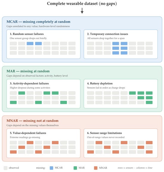
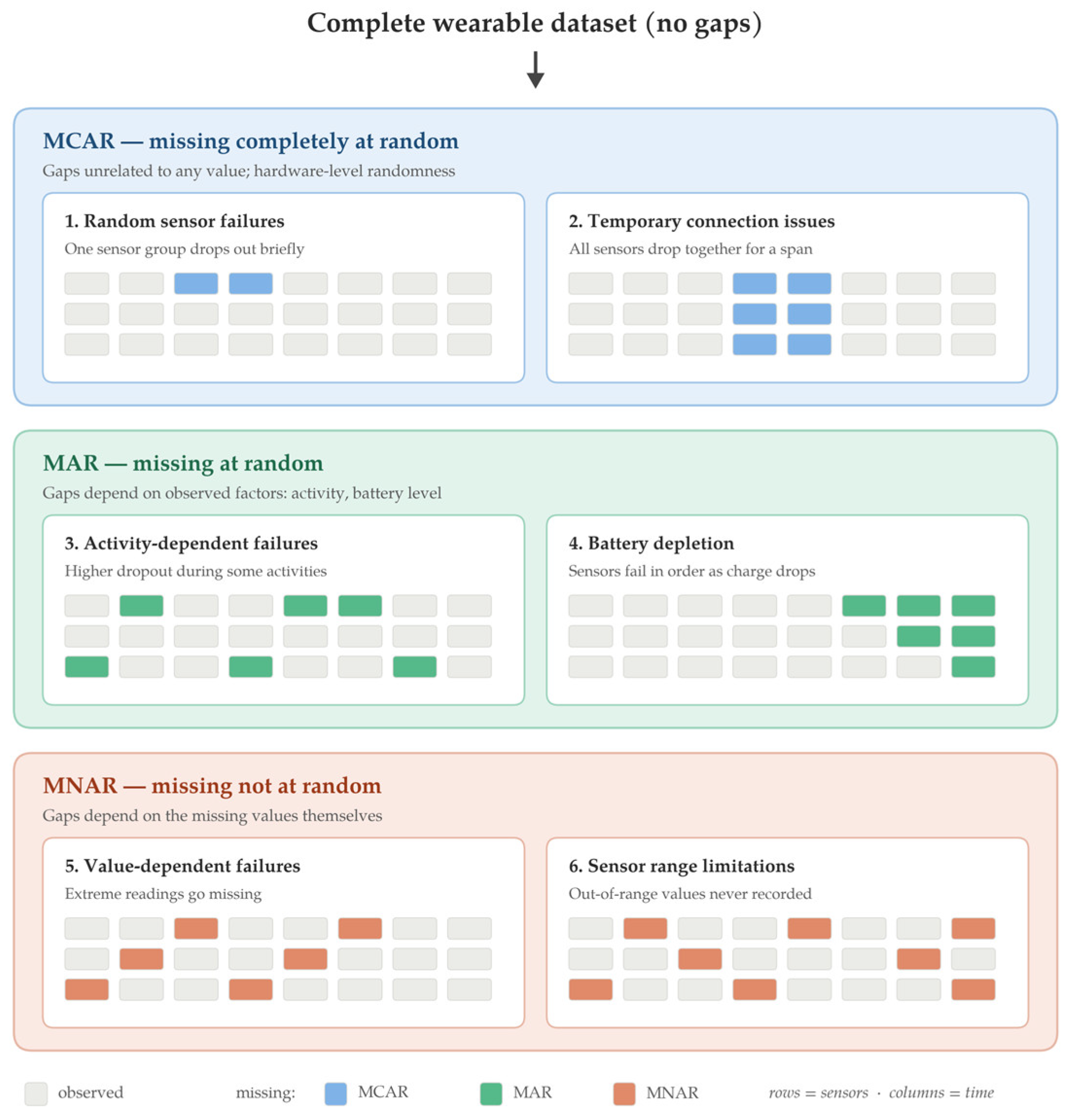
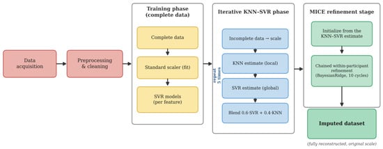
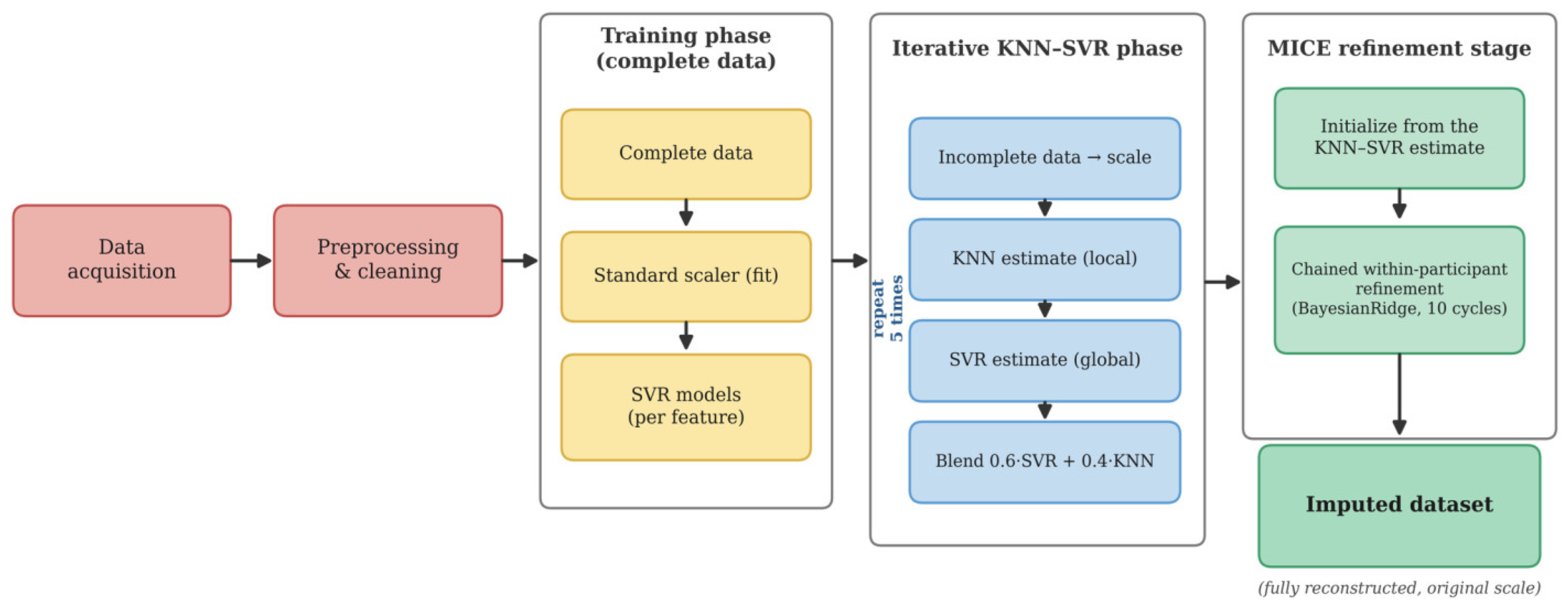
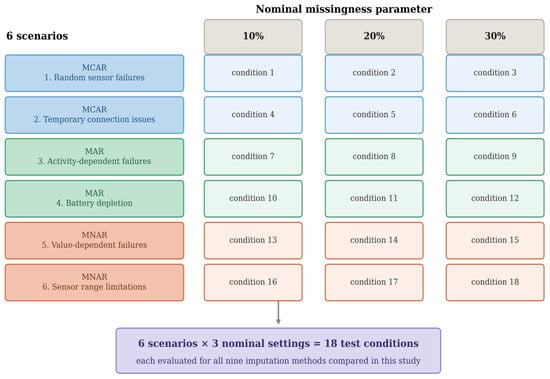
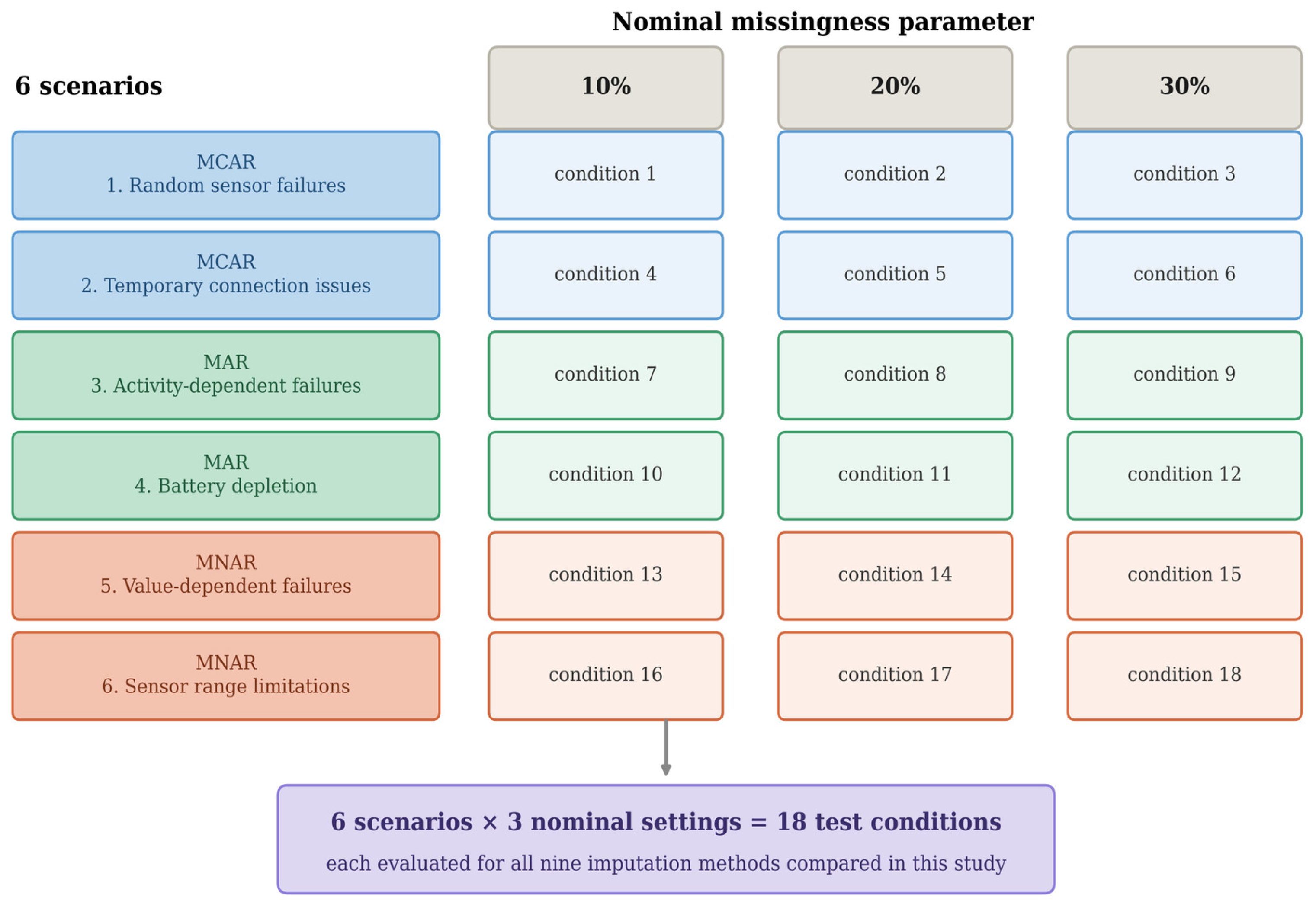
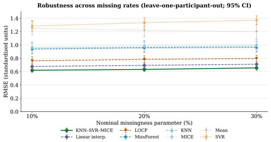
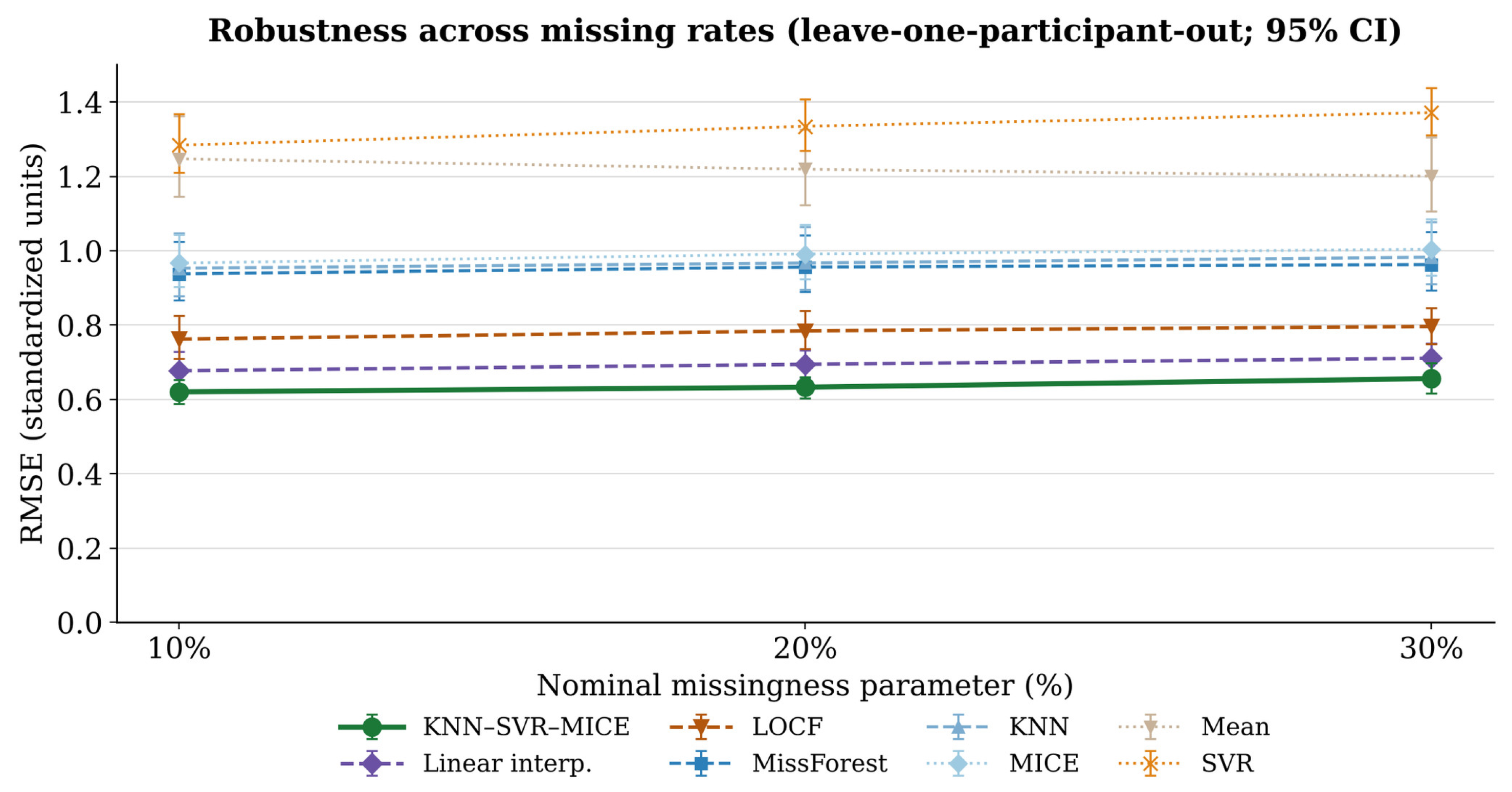
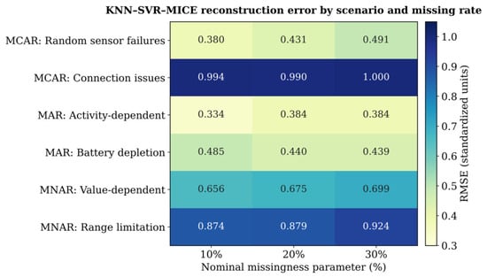
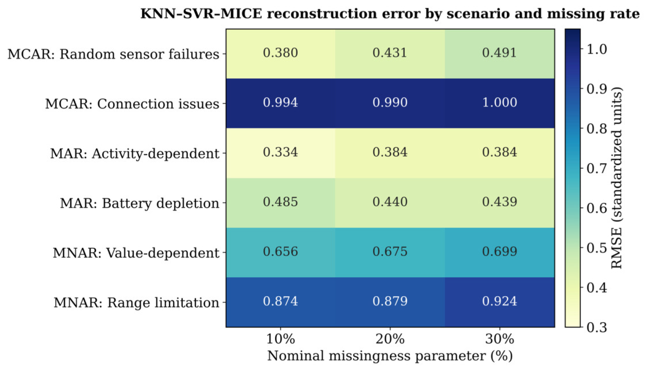

Disclaimer/Publisher’s Note: The statements, opinions and data contained in all publications are solely those of the individual author(s) and contributor(s) and not of MDPI and/or the editor(s). MDPI and/or the editor(s) disclaim responsibility for any injury to people or property resulting from any ideas, methods, instructions or products referred to in the content. |
© 2026 by the authors. Licensee MDPI, Basel, Switzerland. This article is an open access article distributed under the terms and conditions of the Creative Commons Attribution (CC BY) license.