MIMO Radar Waveform Design for Wideband Beampattern with Conjugate Gradient Method on Manifold

Abstract

To tackle the scenario in which a Multiple-Input Multiple-Output (MIMO) radar operates in the presence of interference from other communication systems, this paper investigates wideband waveform design for MIMO radar to enhance beampattern synthesis in a spectrally crowded environment. First, the optimization problem is modeled by minimizing the mean squared error (MSE) for beampattern matching while controlling the energy over specific spatial-frequency spaces (SFSs) to reduce the interference to other systems. Due to the constant modulus (CM) constraint, the resulting problem is non-convex and difficult to handle with conventional optimization methods. Therefore, log-exponential smoothing is applied to construct an exact penalty reformulation of the constrained problem, which is then remodeled on the complex circle manifold and solved efficiently by the Riemannian conjugate gradient (RCG) method. Finally, numerical results show that the proposed method generates deeper nulls in the prescribed SFSs than the counterparts in different scenarios while preserving the beampattern matching accuracy, which demonstrates the superiority of the proposed method.

1. Introduction

Multiple-Input Multiple-Output (MIMO) radar can transmit distinct probing signals, and this waveform diversity offers flexibility for transmit beampattern design, resulting in performance enhancement of target detection [1]. To generate a proper beampattern, a well-designed waveform should be considered [2]. Therefore, waveform design has attracted significant attention in recent years [3,4,5].

Existing research on MIMO radar waveform design can be divided into two categories, i.e., narrowband waveform design [4,5,6,7,8] and wideband waveform design [9,10,11]. The research emphasis of the former is to design a beampattern that focuses the transmit energy on the desired spatial region, while the latter considers both the spatial and the frequency spaces. In practice, such a problem is non-convex and hard to solve because of the constant modulus (CM) constraint. The reason for imposing the CM constraint is that the probing waveform is normalized before being converted to an analog signal by the digital-to-analog converter (DAC), and the discrete-time probing waveform is scaled such that its maximum modulus does not exceed the limits prescribed by the DAC [8].

For narrowband waveform design, in ref. [12], a two-stage method called the cyclic algorithm (CA) is proposed to devise the waveform based on the waveform covariance matrix. In ref. [6], the waveform is directly designed by the alternating direction method of multipliers (ADMM) and the double-ADMM (D-ADMM) methods. However, the modulus of the waveform only continuously approaches a constant with iterations, which means that the designed waveform is not strictly constant modulus. In ref. [8], the authors apply a network-based method to achieve better beampattern performance.

For wideband waveform design, in ref. [9], the authors first optimize the discrete Fourier transform (DFT) matrix of the waveform and then synthesize the transmit waveform so that the DFT of the synthesized waveforms approximates the DFT matrix obtained in the first stage as closely as possible. In ref. [13], a projection-descent-retraction (PDR) method is proposed to solve the problem directly. However, the computation time increases heavily with the waveform length and the number of transmit antennas. In ref. [14], a successive convex approximation method combined with ADMM is developed, where each convex subproblem is solved in closed form; however, selecting suitable penalty factors to guarantee convergence remains challenging. In ref. [15], the majorization–minimization (MM) method is proposed to relax the cost function to ensure convergence to a stationary point, while introducing accuracy errors in beampattern shaping due to the relaxation. In ref. [16], the authors propose the successive alternating projection-ADMM (SAP-ADMM) method to tackle the non-convex optimization problem, at the cost of heavy computational complexity and a non-strict CM property. More recently, in ref. [17], an ADMM-based method with phase parameterization is proposed for joint transmit beampattern and angular waveform synthesis.

The above research all considers beampattern shaping only. Since the application of communication systems is rapidly increasing, they occupy spectrum transmission channels and result in a spectrally crowded environment. Therefore, another constraint should be added, called the spectral constraint [18]. There is much research addressing this problem, but it ignores beampattern synthesis [19,20,21].

To tackle the problem, we first use log-exponential smoothing [22,23] to remodel the optimization problem and then propose a conjugate gradient (CG) optimization method based on the Riemannian manifold optimization framework [24]. In our method, the whole optimization procedure is conducted as an unconstrained optimization problem due to the property of the designed manifold, and all the iterates are restricted on the complex circle manifold, so that the designed waveform is strictly constant modulus. To make the designed waveform applicable in practical engineering, we utilize the 1D search method [25] to generate a discrete phase coding waveform based on the designed waveform. In the numerical results, compared with MM in ref. [15] and SAP-ADMM in ref. [16], our proposed method can generate deeper nulls in the desired spatial-frequency space (SFS) efficiently while preserving the beampattern performance. The main contributions of this paper are summarized as follows:

• We formulate the wideband MIMO radar beampattern matching problem with spatial spectral nulling (SSN) constraints and the CM constraint and transform it into an unconstrained problem on the complex circle product manifold by a log-exponential smoothing exact penalty, in which the penalty factor and the smoothing parameter are adaptively updated with a specific criterion.
• We develop an RCG method to solve the reformulated problem, where the Polak–Ribiére parameter, vector transport, Armijo line search and retraction are derived for the product manifold. All iterates strictly satisfy the CM constraint, and the per-iteration complexity is low since no matrix inversion is required.
• Numerical results in two interference scenarios show that, compared with the MM method and the SAP-ADMM method, the proposed method generates much deeper nulls in the desired SFSs with almost the same beampattern matching accuracy, while reducing the computation time significantly. In particular, thanks to the manifold optimization framework, the designed waveform is strictly constant modulus (the modulus error is zero up to machine precision), unlike the SAP-ADMM method whose waveform only approaches a constant modulus. In addition, the performance is well preserved when the designed waveform is quantized to a 64-phase coding waveform.

Notation: We adopt the notation of using boldface for vectors $\mathit{a}$ (lower case), and matrices $\mathbf{A}$ (upper case). The transpose, conjugate, conjugate transpose operators, are denoted by the symbols ${(·)}^T$, ${(·)}^{*}$ and ${(·)}^H$, respectively. $\left|·\right|$ denotes the modulus of a complex number. ${∥·∥}_2$ denotes the 2-norm of a vector. The n-th element of a vector $\mathit{a}$ is written as $a\left(n\right)$. $vec\left(\mathbf{A}\right)$ is the vectorization of matrix $\mathbf{A}$. The sets of $N\times N$ complex matrices and N-dimensional complex vectors are denoted by ${\mathbb{C}}^{N\times N}$ and ${\mathbb{C}}^N$, respectively. The sets of $N\times N$ real matrices and N-dimensional real vectors are denoted by ${\mathbb{R}}^{N\times N}$ and ${\mathbb{R}}^N$, respectively. ${\mathbf{I}}_N$ denotes the $N\times N$ identity matrix. $\mathrm{Re}\{·\}$ denotes the real part of a complex number. Finally, we use the symbol ⊗ for the Kronecker product, and the symbol ⊙ for element-wise multiplication.

2. System Model

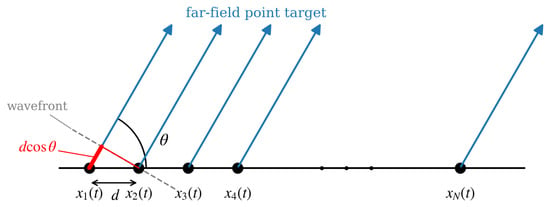
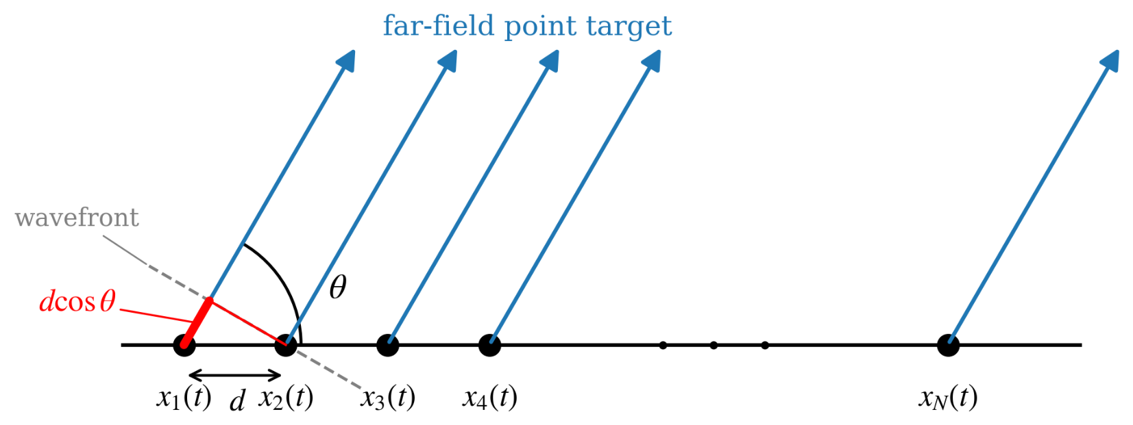
Consider a wideband MIMO radar system equipped with a uniform linear array (ULA) of N elements with inter-element spacing d, as shown in Figure 1. The bandpass signal emitted by the n-th antenna is

$$x_n\left(t\right)=\mathrm{Re}\left\{s_n\left(t\right)e^{j2\pi f_{c}t}\right\},n=1,2,\cdots ,N,$$

(1)

where $s_n\left(t\right)$ is the complex envelope (baseband waveform) of the n-th transmit signal, and $f_c$ is the carrier frequency. The spectral support of the complex envelope $s_n\left(t\right)$ is assumed to be within the interval $\left[-B/2,B/2\right]$; i.e., B is the bandwidth of the bandpass signal $x_n\left(t\right)$. For a far-field point target at the spatial angle $\theta$ measured from the array axis, the signal synthesized at the target is the superposition of the signals transmitted by all the elements, which can be written as

$$\begin{array}{c}r\left(t\right)={\displaystyle \sum _{n=1}^N}{x}_n(t-{\tau }_n)\hfill \\ ={\displaystyle \sum _{n=1}^N}\mathrm{Re}\left\{s_n(t-{\tau }_n)e^{j2\pi f_c(t-{\tau }_n)}\right\},\hfill \end{array}$$

(2)

where c represents the speed of light, and ${\tau }_n={\displaystyle \frac{(N-n)d\cos \theta }{c}}$ is the propagation delay of the signal transmitted by the n-th element relative to that transmitted by the reference element. Here, the last element (the N-th element) is taken as the reference element, since, for the geometry illustrated in Figure 1, its signal has the shortest propagation path to the target. Specifically, the propagation path from the n-th element to the target is longer than that from the N-th element by $(N-n)d\cos \theta$, so that ${\tau }_n\ge 0$ is a genuine time delay: the signal emitted by the N-th element arrives at the target first (${\tau }_N=0$), while the signal emitted by the first element has the largest delay ${\tau }_1=(N-1)d\cos \theta /c$. Note that the common propagation delay from the reference element to the far-field target is omitted in (2), since it only introduces a common phase rotation in $r\left(t\right)$ and does not affect the transmit beampattern.

Figure 1. Uniform linear array of the wideband MIMO radar and the far-field signal model.

After down-conversion, the complex envelope $s_n\left(t\right)$ is sampled with the sampling interval $T_c=1/B$, which yields the discrete-time baseband sequence $s_n\left(l\right)\triangleq s_n\left(l{T}_c\right)$, $l=0,1,\cdots ,L-1$, where L is the number of time samples. The frequency-domain representation of $s_n\left(l\right)$ is obtained by the L-point discrete Fourier transform (DFT):

$$y_n\left(p\right)={\displaystyle \sum _{l=0}^{L-1}}{s}_n\left(l\right)e^{-j2\pi {\displaystyle \frac{lp}{L}}},p=-{\displaystyle \frac{L}{2}},-{\displaystyle \frac{L}{2}}+1,\cdots ,{\displaystyle \frac{L}{2}}-1,$$

(3)

where the p-th frequency bin corresponds to the frequency $f_p=f_c+{\displaystyle \frac{p}{L{T}_c}}$. By dividing the spatial angle interval $\left[0^{\circ },{180}^{\circ }\right]$ into K grid points, the steering vector at angle $\theta$ and frequency $f_p$ can be given by

$$\mathit{a}(\theta ,f_p)={\displaystyle \frac{1}{\sqrt{N}}}{\left[e^{j2\pi f_p{\tau }_1},e^{j2\pi f_p{\tau }_2},\cdots ,e^{j2\pi f_p{\tau }_N}\right]}^T,$$

(4)

where ${\tau }_n=(N-n)d\cos \theta /c$ is the delay defined in (2). Note that (4) differs from the steering vector referenced at the first element only by a common phase factor $e^{j2\pi f_p(N-1)d\cos \theta /c}$, which does not affect the beampattern in (5). The discrete-frequency beampattern in the far field at angle ${\theta }_k$ and frequency $f_p$ is

$$P\left({\theta }_k,f_p\right)={\left|{\mathit{a}}^H\left({\theta }_k,f_p\right){\mathit{y}}_p\right|}^2,$$

(5)

where ${\mathit{y}}_p={\left[y_1\left(p\right),y_2\left(p\right),\cdots ,y_N\left(p\right)\right]}^T$ collects the p-th DFT coefficients of all antennas. Let ${\mathit{s}}_l={\left[s_1\left(l\right),s_2\left(l\right),\cdots ,s_N\left(l\right)\right]}^T$ denote the l-th sample of all antennas and $\mathit{s}={\left[{\mathit{s}}_0^T,{\mathit{s}}_1^T,\cdots ,{\mathit{s}}_{L-1}^T\right]}^T\in {\mathbb{C}}^{NL}$ collect all the waveform samples. Then, the DFT in (3) can be written in a compact form, and the discrete-frequency beampattern can be denoted as

$$P\left({\theta }_k,f_p\right)={\left|{\mathit{a}}^H\left({\theta }_k,f_p\right){\mathbf{F}}_p\mathit{s}\right|}^2,$$

(6)

where ${\mathbf{F}}_p={\mathit{e}}_p\otimes {\mathbf{I}}_N\in {\mathbb{C}}^{N\times NL}$ and ${\mathit{e}}_p={\displaystyle \frac{1}{\sqrt{L}}}\left[1,e^{-j2\pi {\displaystyle \frac{p}{L}}},\cdots ,e^{-j2\pi {\displaystyle \frac{(L-1)p}{L}}}\right]$ is the p-th DFT vector, such that ${\mathbf{F}}_p\mathit{s}={\displaystyle \frac{1}{\sqrt{L}}}{\mathit{y}}_p$.

Assume that the whole discrete space-frequency region is represented as $\left({\theta }_k,f_p\right)\in \mathrm{\Theta }$. A beampattern matching problem for a wideband MIMO radar can then be formulated as follows:

$$\begin{array}{c}\underset{\mathit{s}}{\min }{\displaystyle \sum _{k=1}^K}{\displaystyle \sum _{p=-L/2}^{L/2-1}}{\left[d_{kp}-\left|{\mathbf{a}}^H\left({\theta }_k,f_p\right){\mathbf{F}}_p\mathit{s}\right|\right]}^2\hfill \\ \mathrm{s}.\mathrm{t}.\left|s\left(i\right)\right|=1,i=1,2,\cdots ,NL,\hfill \end{array}$$

(7)

where $d_{kp}=\epsilon {\overline{d}}_{kp}{e}^{j{\phi }_{kp}}$, ${\overline{d}}_{kp}$ is the desired beampattern at $({\theta }_k,f_p)$. Following [15,16], the matching is performed up to a scaling factor $\epsilon$ and a matching phase ${\phi }_{kp}$, which are given by

$$\left\{\begin{array}{cc}\hfill {\phi }_{kp}& =\arg \left\{{\mathbf{a}}^H({\theta }_k,f_p){\mathbf{F}}_p\mathit{s}\right\},\hfill \\ \hfill \epsilon & ={\displaystyle \frac{{\displaystyle \sum _{k=1}^K}{\displaystyle \sum _{p=-L/2}^{L/2-1}}\left|{\mathbf{a}}^H({\theta }_k,f_p){\mathbf{F}}_p\mathit{s}\right|}{{\displaystyle \sum _{k=1}^K}{\displaystyle \sum _{p=-L/2}^{L/2-1}}{\overline{d}}_{kp}}}.\hfill \end{array}\right.$$

(8)

Aside from beampattern matching, another optimization target is the energy spectral density (ESD). Suppose there are M communication systems in a spectrum-crowded environment, and the space-frequency region occupied by the m-th communication system is denoted by ${\mathrm{\Theta }}_m$. It is necessary to impose a limitation on the ESD over ${\mathrm{\Theta }}_m$ to achieve the coexistence of the wideband MIMO radar and the communication systems, which can be given by

$$\sum _{({\theta }_k^m,f_p^m)\in {\mathrm{\Theta }}_m}{\left|{\mathbf{a}}^H\left({\theta }_k^m,f_p^m\right){\mathbf{F}}_p\mathit{s}\right|}^2\le {\varsigma }_m,m=1,2,\cdots ,M,$$

(9)

where ${\varsigma }_m$ is the parameter that controls the ESD over the m-th region: a smaller ${\varsigma }_m$ enforces a stronger suppression and hence a deeper null. Combining (7) and (9), the overall optimization problem can be modeled as

$$\begin{array}{c}\underset{\mathit{s}}{\min }{\displaystyle \sum _{k=1}^K}{\displaystyle \sum _{p=-L/2}^{L/2-1}}{\left[d_{kp}-\left|{\mathbf{a}}^H\left({\theta }_k,f_p\right){\mathbf{F}}_p\mathit{s}\right|\right]}^2\hfill \\ \mathrm{such}\mathrm{that}{\displaystyle \sum _{({\theta }_k^m,f_p^m)\in {\mathrm{\Theta }}_m}}{\left|{\mathbf{a}}^H\left({\theta }_k^m,f_p^m\right){\mathbf{F}}_p\mathit{s}\right|}^2\le {\varsigma }_m,m=1,2,\cdots ,M,\hfill \\ \left|s\left(i\right)\right|=1,i=1,2,\cdots ,NL.\hfill \end{array}$$

(10)

Remark 1.

The MSE (least-squares) criterion is adopted in (7) and (10) for beampattern matching. It is widely used in (wideband) MIMO radar beampattern design [9,14,15,16,26] for the following reasons. First, the MSE directly measures the average matching fidelity over the whole angle-frequency region and leads to a smooth quartic objective whose gradient has a closed form, which enables efficient on-manifold optimization with $\mathcal{O}\left({\left(NL\right)}^2\right)$ complexity per iteration. In contrast, a min–max formulation that directly controls the peak sidelobe level (PSL) or the mainlobe/sidelobe ripple is non-smooth and has to be handled by log-exponential smoothing or weighted $l_p$-norm approximations [4,23], which introduces extra hyperparameters and a higher computational burden, and the solution is sensitive to the grid density. Second, since the CM waveform only provides $NL$ degrees of freedom, while the beampattern is evaluated over $K\times L$ grid points with $K\times L\gg NL$, the achievable PSL is fundamentally limited; minimizing the MSE spreads the matching error evenly over the region of interest, which in practice also leads to low sidelobes. Third, the hard SSN constraints in (9) already provide a worst-case control of the radiated energy in the critical regions, which covers the practical requirement that a min–max criterion would serve. The min–max design for the wideband beampattern synthesis will be considered in our future work.

Remark 2.

In this paper, the beampattern is modeled with the azimuth angle θ only, i.e., a planar model is considered with a ULA. This is a common assumption in wideband MIMO radar beampattern design [9,14,15,16]. For real-world systems where the terrain is not flat, and the elevation angle matters, the proposed formulation can be extended in a straightforward manner by replacing the ULA steering vector with that of a planar or volumetric array, in which case the steering vector depends on both the azimuth and elevation angles, and the manifold structure as well as the proposed RCG method remain unchanged. The two-dimensional extension will be investigated in our future work.

3. The Proposed Method

In this section, we first remodel the problem on the Riemannian manifold by exploiting the CM property. Then, a log-exponential smoothing function is applied to smooth the optimization problem. Finally, the Riemannian conjugate gradient (RCG) method is used to solve the problem efficiently.

3.1. Reformulated Optimization Problem

The CM constraint in (10) describes the Cartesian product of $NL$ complex circles. Let $\mathcal{M}$ denote this product manifold,

$$\mathcal{M}=\{\mathit{s}\in {\mathbb{C}}^{NL}:\left|s\left(i\right)\right|=1,i=1,2,\cdots ,NL\}.$$

(11)

Then, the CM-constrained optimization problem can be viewed as an unconstrained optimization problem over $\mathcal{M}$. For a point $\mathit{s}$ on $\mathcal{M}$, a tangent vector at $\mathit{s}$ is tangent to any smooth curve on $\mathcal{M}$ passing through $\mathit{s}$. The set of all such vectors at $\mathit{s}$ forms the tangent space, denoted by ${\mathrm{T}}_{\mathit{s}}\mathcal{M}$, which is a Euclidean space:

$${\mathrm{T}}_{\mathit{s}}\mathcal{M}=\left\{{\mathit{\epsilon }}_{\mathit{s}}\in {\mathbb{C}}^{NL}:\mathrm{Re}\{{\mathit{\epsilon }}_{\mathit{s}}\odot {\mathit{s}}^{*}\}={\mathbf{0}}_{NL}\right\},$$

(12)

where ${\mathit{\epsilon }}_{\mathit{s}}$ denotes a tangent vector at the point $\mathit{s}$, and ${\mathbf{0}}_{NL}$ denotes the $NL$-dimensional zero vector. Then, (10) can be transformed as follows:

$$\begin{array}{c}\underset{\mathit{s}}{\min }{\displaystyle \sum _{k=1}^K}{\displaystyle \sum _{p=-L/2}^{L/2-1}}{\left[d_{kp}-\left|{\mathbf{a}}^H\left({\theta }_k,f_p\right){\mathbf{F}}_p\mathit{s}\right|\right]}^2\hfill \\ \mathrm{s}.\mathrm{t}.{\displaystyle \sum _{({\theta }_k^m,f_p^m)\in {\mathrm{\Theta }}_m}}{\left|{\mathbf{a}}^H\left({\theta }_k^m,f_p^m\right){\mathbf{F}}_p\mathit{s}\right|}^2\le {\varsigma }_m,m=1,2,\cdots ,M,\hfill \\ \mathit{s}\in \mathcal{M}.\hfill \end{array}$$

(13)

Next, we introduce the maximum function to handle the inequality constraints:

$$\begin{array}{cc}\hfill L_m\left(\mathit{s}\right)& =\max (0,\sum _{({\theta }_k^m,f_p^m)\in {\mathrm{\Theta }}_m}{\left|{\mathbf{a}}^H({\theta }_k^m,f_p^m){\mathbf{F}}_p\mathit{s}\right|}^2-{\varsigma }_m),\hfill \\ & \hspace{1em}\hspace{1em}\hspace{1em}m=1,2,\cdots ,M.\hfill \end{array}$$

(14)

Notice that the log-exponential smoothing function satisfies [23]

$$\max \{a,b\}\approx \lambda \ln \left[e^{{\displaystyle \frac{a}{\lambda }}}+e^{{\displaystyle \frac{b}{\lambda }}}\right],$$

(15)

where $\lambda >0$ is the smoothing parameter, and a and b are real numbers. Let $C_1\left(\mathit{s}\right)={\displaystyle \sum _{k=1}^K}{\displaystyle \sum _{p=-L/2}^{L/2-1}}{\left[d_{kp}-\left|{\mathbf{a}}^H\left({\theta }_k,f_p\right){\mathbf{F}}_p\mathit{s}\right|\right]}^2$ and $C_2{\left(\mathit{s}\right)}_m={\displaystyle \sum _{({\theta }_k^m,f_p^m)\in {\mathrm{\Theta }}_m}}{\left|{\mathbf{a}}^H\left({\theta }_k^m,f_p^m\right){\mathbf{F}}_p\mathit{s}\right|}^2-{\varsigma }_m$. According to (11)–(15), the problem is formulated as follows:

$$\underset{\mathit{s}\in \mathcal{M}}{\min }f\left(\mathit{s}\right)=C_1\left(\mathit{s}\right)+\rho \lambda {\displaystyle \sum _{m=1}^M}\ln \left(1+e^{\left({\displaystyle \frac{C_2{\left(\mathit{s}\right)}_m}{\lambda }}\right)}\right),$$

(16)

where $\rho$ is a penalty factor. Note that, due to the smoothing, the optimal solution of problem (16) may not coincide with that of the original problem (10). However, there exist proper values of $\rho$ and $\lambda$ such that the solution of (16) meets that of (10). In our proposed method, $\rho$ and $\lambda$ are updated through iterations with a specific criterion, which leads to a continuously approaching optimal solution.

3.2. RCG Method

With fixed $\rho$ and $\lambda$, we apply the RCG method to solve (16). First, we compute the Riemannian gradient $\mathrm{grad}f\left(\mathit{s}\right)$, which satisfies

$$g_{\mathit{s}}\left({\mathit{\epsilon }}_{\mathit{s}},\mathrm{grad}f\left(\mathit{s}\right)\right)=Df\left(\mathit{s}\right)\left[{\mathit{\epsilon }}_{\mathit{s}}\right],\forall {\mathit{\epsilon }}_{\mathit{s}}\in {\mathrm{T}}_{\mathit{s}}\mathcal{M},$$

(17)

where $g_{\mathit{s}}(·,·)$ denotes the Riemannian metric at $\mathit{s}$, and

$$Df\left(\mathit{s}\right)\left[{\mathit{\epsilon }}_{\mathit{s}}\right]=\underset{t\to 0}{\lim }{\displaystyle \frac{f\left(\mathit{s}+t{\mathit{\epsilon }}_{\mathit{s}}\right)-f\left(\mathit{s}\right)}{t}}$$

(18)

denotes the directional derivative of $f\left(\mathit{s}\right)$ at $\mathit{s}$. Let $\nabla f$ denote the Euclidean gradient of $f\left(\mathit{s}\right)$. Then, the Riemannian gradient of $f\left(\mathit{s}\right)$ can be computed by

$$\begin{array}{c}\mathrm{grad}f\left(\mathit{s}\right)={\mathrm{Proj}}_{{\mathrm{T}}_{\mathit{s}}\mathcal{M}}\left(\nabla f\right)\hfill \\ =\nabla f-\mathrm{Re}\left\{\nabla f\odot {\mathit{s}}^{*}\right\}\odot \mathit{s},\hfill \end{array}$$

(19)

where ${\mathrm{Proj}}_{{\mathrm{T}}_{\mathit{s}}\mathcal{M}}\left(\nabla f\right)$ denotes the orthogonal projection of $\nabla f$ onto ${\mathrm{T}}_{\mathit{s}}\mathcal{M}$. $\nabla f$ is computed by

$${\nabla }_{\mathit{s}}f\left(\mathit{s}\right)={\nabla }_{\mathit{s}}{C}_1\left(\mathit{s}\right)+\rho {\displaystyle \sum _{m=1}^M}{\displaystyle \frac{1}{1+e^{-\frac{C_2{\left(\mathit{s}\right)}_m}{\lambda }}}}{\nabla }_{\mathit{s}}{C}_2{\left(\mathit{s}\right)}_m.$$

(20)

Let ${\mathbf{A}}_p={\left[\mathbf{a}({\theta }_1,f_p),\mathbf{a}({\theta }_2,f_p),\cdots ,\mathbf{a}({\theta }_K,f_p)\right]}^H$ and ${\mathit{d}}_p={\left[d_{1p}{e}^{j{\phi }_{1p}},d_{2p}{e}^{j{\phi }_{2p}},\cdots ,d_{Kp}{e}^{j{\phi }_{Kp}}\right]}^T$. Notice that $C_1\left(\mathit{s}\right)$ can be written as [13,15]

$$\begin{array}{c}{C}_1\left(\mathit{s}\right)={\displaystyle \sum _p}{∥{\mathit{d}}_p-{\mathbf{A}}_p{\mathbf{F}}_p\mathit{s}∥}_2^2\hfill \\ ={\displaystyle \sum _p}{\mathit{s}}^H{\mathbf{F}}_p^H{\mathbf{A}}_p^H{\mathbf{A}}_p{\mathbf{F}}_p\mathit{s}-{\mathit{d}}_p^H{\mathbf{A}}_p{\mathbf{F}}_p\mathit{s}-{\mathit{s}}^H{\mathbf{F}}_p^H{\mathbf{A}}_p^H{\mathit{d}}_p+\hfill \\ {\displaystyle \sum _p}{\mathit{d}}_p^H{\mathit{d}}_p\hfill \\ ={\mathit{s}}^H\left({\displaystyle \sum _p}{\mathbf{F}}_p^H{\mathbf{A}}_p^H{\mathbf{A}}_p{\mathbf{F}}_p\right)\mathit{s}-\left({\displaystyle \sum _p}{\mathit{d}}_p^H{\mathbf{A}}_p{\mathbf{F}}_p\right)\mathit{s}-\hfill \\ {\mathit{s}}^H\left({\displaystyle \sum _p}{\mathbf{F}}_p^H{\mathbf{A}}_p^H{\mathit{d}}_p\right)+{\displaystyle \sum _p}{\mathit{d}}_p^H{\mathit{d}}_p\hfill \\ ={\mathit{s}}^H\mathbf{P}\mathit{s}-{\mathit{q}}^H\mathit{s}-{\mathit{s}}^H\mathit{q}+r,\hfill \end{array}$$

(21)

where $\mathbf{P}={\displaystyle \sum _p}{\mathbf{F}}_p^H{\mathbf{A}}_p^H{\mathbf{A}}_p{\mathbf{F}}_p$, $\mathit{q}={\displaystyle \sum _p}{\mathbf{F}}_p^H{\mathbf{A}}_p^H{\mathit{d}}_p$ and $r={\displaystyle \sum _p}{\mathit{d}}_p^H{\mathit{d}}_p$.

Therefore, ${\nabla }_{\mathit{s}}{C}_1\left(\mathit{s}\right)$ can be given by

$${\nabla }_{\mathit{s}}{C}_1\left(\mathit{s}\right)=2\mathbf{P}\mathit{s}-2\mathit{q}.$$

(22)

Similarly, $C_2{\left(\mathit{s}\right)}_m$ can be written as

$$C_2{\left(\mathit{s}\right)}_m={\mathit{s}}^H{\mathbf{P}}_m\mathit{s}-{\varsigma }_m,$$

(23)

where ${\mathbf{P}}_m={\displaystyle \sum _{\left({\theta }_k^m,f_p^m\right)\in {\mathrm{\Theta }}_m}}{\mathbf{F}}_p^H\mathbf{a}\left({\theta }_k^m,f_p^m\right){\mathit{a}}^H\left({\theta }_k^m,f_p^m\right){\mathbf{F}}_p$. Therefore, ${\nabla }_{\mathit{s}}{C}_2{\left(\mathit{s}\right)}_m$ can be given by

$${\nabla }_{\mathit{s}}{C}_2{\left(\mathit{s}\right)}_m=2{\mathbf{P}}_m\mathit{s}.$$

(24)

After computing the Riemannian gradient, the RCG algorithm can be applied to solve the problem. In Euclidean space, the search direction of the CG method [27] can be given by

$${\mathit{d}}_k=-{\nabla }_{\mathit{s}}f\left({\mathit{s}}_k\right)+u_{k-1}{\mathit{d}}_{k-1}.$$

(25)

Similarly, in Riemannian space, the conjugate direction can be given by

$${\mathit{d}}_{{\mathit{s}}_k}=-\mathrm{grad}f\left({\mathit{s}}_k\right)+u_{k-1}{\mathrm{Trans}}_{{\mathit{s}}_k\leftarrow {\mathit{s}}_{k-1}}\left({\mathit{d}}_{{\mathit{s}}_{k-1}}\right),$$

(26)

where $\mathrm{Trans}$ denotes the vector transport, which transports the tangent vector ${\mathit{d}}_{{\mathit{s}}_{k-1}}$ from the point ${\mathit{s}}_{k-1}\in \mathcal{M}$ to another point ${\mathit{s}}_k\in \mathcal{M}$. The vector transport is realized by the orthogonal projection of ${\mathit{d}}_{{\mathit{s}}_{k-1}}$ onto ${\mathrm{T}}_{{\mathit{s}}_k}\mathcal{M}$:

$$\begin{array}{cc}\hfill {\mathrm{Trans}}_{{\mathit{s}}_k\leftarrow {\mathit{s}}_{k-1}}\left({\mathit{d}}_{{\mathit{s}}_{k-1}}\right)& ={\mathrm{Proj}}_{{\mathrm{T}}_{{\mathit{s}}_k}\mathcal{M}}\left({\mathit{d}}_{{\mathit{s}}_{k-1}}\right)\hfill \\ \hfill & ={\mathit{d}}_{{\mathit{s}}_{k-1}}-\mathrm{Re}\left\{{\mathit{d}}_{{\mathit{s}}_{k-1}}\odot {\mathit{s}}_k^{*}\right\}\odot {\mathit{s}}_k.\hfill \end{array}$$

(27)

$u_{k-1}$ is chosen as the Polak–Ribière parameter [28], which is given by

$$u_{k-1}={\displaystyle \frac{⟨\mathrm{grad}f\left({\mathit{s}}_k\right),\mathrm{grad}f\left({\mathit{s}}_k\right)-{\mathrm{Proj}}_{{\mathrm{T}}_{{\mathit{s}}_k}\mathcal{M}}\left(\mathrm{grad}f\left({\mathit{s}}_{k-1}\right)\right)⟩}{⟨\mathrm{grad}f\left({\mathit{s}}_{k-1}\right),\mathrm{grad}f\left({\mathit{s}}_{k-1}\right)⟩}},$$

(28)

where $⟨·,·⟩$ is the Riemannian metric [24], which is commonly defined as

$$⟨\mathit{\epsilon },\mathit{\eta }⟩=\mathrm{Re}\left\{{\mathit{\epsilon }}^H\mathit{\eta }\right\}.$$

(29)

Then, the update formula of the RCG method can be given by

$${\mathit{s}}_{k+1}={\mathfrak{R}}_{{\mathit{s}}_k}\left(t_k{\mathit{d}}_{{\mathit{s}}_k}\right),$$

(30)

where

$${\mathfrak{R}}_{\mathit{s}}\left({\mathit{\epsilon }}_{\mathit{s}}\right)={\displaystyle \frac{\mathit{s}+{\mathit{\epsilon }}_{\mathit{s}}}{\left|\mathit{s}+{\mathit{\epsilon }}_{\mathit{s}}\right|}}$$

(31)

is the retraction that maps a tangent vector back onto the manifold $\mathcal{M}$, with the division and modulus taken element-wise, and $t_k$ is the step size determined by the Armijo line search [29]. The overall RCG procedure for solving (16) with fixed $\rho$ and $\lambda$ is summarized in Algorithm 1.

Algorithm 1 The RCG algorithm for solving problem (16) with fixed $\rho$ and $\lambda$.

Input:  Initial point ${\mathit{s}}_0\in \mathcal{M}$. Output:  Optimized waveform ${\mathit{s}}_{opt}$.   1: Initialize $k=1$, compute ${\mathit{d}}_{{\mathit{s}}_0}=-\mathrm{grad}f\left({\mathit{s}}_0\right)$ by (19), and set ${\mathit{s}}_1={\mathfrak{R}}_{{\mathit{s}}_0}\left(t_0{\mathit{d}}_{{\mathit{s}}_0}\right)$.   2: Compute the step size $t_k$ by the Armijo line search.   3: Update ${\mathit{s}}_{k+1}$ by (30) and (26), and compute $\mathrm{grad}f\left({\mathit{s}}_{k+1}\right)$ by (19).   4: Transport ${\mathit{d}}_{{\mathit{s}}_k}$ to the tangent space ${\mathrm{T}}_{{\mathit{s}}_{k+1}}\mathcal{M}$ by (27).   5: Compute $u_k$ by (28) and let $k=k+1$.   6: If ${∥\mathrm{grad}f\left({\mathit{s}}_{k+1}\right)∥}_2\le {ϵ}_{\mathrm{tol}}$, where ${ϵ}_{\mathrm{tol}}$ is a parameter to control convergence, output ${\mathit{s}}_{opt}={\mathit{s}}_{k+1}$; otherwise, repeat Step 2.

3.3. Update of $\rho$ and $\lambda$

In the proposed method, $\rho$ is initialized as a relatively small value to avoid a high computational cost for achieving a feasible solution. A possible approach is to increase $\rho$ iteratively while decreasing $\lambda$ to reduce the smoothing error. First, let us consider the proper value of $\lambda$. The log-exponential smoothing performs an interesting property, which can be given by [23]

$$\max \left\{a,b\right\}\le \lambda \ln \left[e^{{\displaystyle \frac{a}{\lambda }}}+e^{{\displaystyle \frac{b}{\lambda }}}\right]\le \lambda \ln \left(2\right)+\max \left\{a,b\right\}.$$

(32)

From (32), it is obvious that the smoothing accuracy can be enhanced with a smaller $\lambda$. However, it is necessary to set $\lambda >{\lambda }_{\min }$ to prevent numerical difficulty [30]. The initial value of $\lambda$ can be set to a relatively large value to accelerate the convergence speed. The update rule of $\lambda$ is given by

$${\lambda }_{t+1}=\max \left\{{\lambda }_{\min },\alpha {\lambda }_t\right\},$$

(33)

where $\alpha \in \left(0,1\right)$ is a positive constant fraction to decrease $\lambda$.

In the t-th iteration, we can obtain ${\mathit{s}}_{t+1}$ through the RCG method in Algorithm 1. Therefore, we can calculate the maximum value of the constraint functions as

$$E\left({\mathit{s}}_{t+1}\right)=\max \left\{C_2{\left({\mathit{s}}_{t+1}\right)}_m,m=1,2,\cdots ,M\right\}.$$

(34)

If $E\left({\mathit{s}}_{t+1}\right)\ge {\lambda }_t$, $\rho$ is updated as

$${\rho }_{t+1}={\displaystyle \frac{{\rho }_t}{\beta }},$$

(35)

where $\beta \in \left(0,1\right)$ is the scaling factor of $\rho$.

3.4. The Whole Optimization Method

Finally, the whole optimization procedure is summarized in Algorithm 2.

Algorithm 2 The proposed method to solve problem (10).

Input:  Initial point ${\mathit{s}}_0\in \mathcal{M}$, ${\rho }_0$, ${\lambda }_0$, $\alpha$, $\beta$, iterative counting parameter $t=0$. Output:  Optimized waveform ${\mathit{s}}_{opt}$.   1: Compute ${\mathit{s}}_{t+1}$ with the RCG method in Algorithm 1.   2: Compute $\delta ={∥{\mathit{s}}_{t+1}-{\mathit{s}}_t∥}_2$. If $\delta <{\delta }_{\min }$, then output ${\mathit{s}}_{opt}={\mathit{s}}_{t+1}$; otherwise, go to Step 3.   3: Compute ${\lambda }_{t+1}=\max \{{\lambda }_{\min },\alpha {\lambda }_t\}$;   4: If $E\left({\mathit{s}}_{t+1}\right)\ge {\lambda }_t$, then compute ${\rho }_{t+1}$ according to (35); otherwise, let ${\rho }_{t+1}={\rho }_t$.   5: Return to Step 1.

To make the designed waveform applicable in practical engineering, we apply the 1D search method [25] to generate a discrete phase coding waveform based on the designed waveform. Let $\tilde{K}$ denote the total phase coding number and ${\varphi }_i$ denote the phase of the i-th component of ${\mathit{s}}_{opt}$. The procedure can be denoted by

$$\begin{array}{c}{\tilde{\varphi }}_i=\underset{{\tilde{\varphi }}_i}{\arg \min }{\left({\tilde{\varphi }}_i-{\varphi }_i\right)}^2\hfill \\ \mathrm{s}.\mathrm{t}.{\tilde{\varphi }}_i\in {\displaystyle \frac{2\pi }{\tilde{K}}}\{1,\cdots ,\tilde{K}\},\hfill \end{array}$$

(36)

where ${\tilde{\varphi }}_i$ is the quantized phase. Applying the above procedure to all components, the optimized discrete phase coding waveform ${\tilde{\mathit{s}}}_{opt}$ can be obtained.

4. Numerical Results

In this section, numerical results are carried out through the following aspects: 1. the convergence of the proposed algorithm; 2. the nulling performance with different values of $\varsigma$; 3. the beampattern performance with the discrete phase coding waveform; 4. the performance comparison with the MM method [15] and the SAP-ADMM method [16]; 5. the designed waveforms.

In all simulations, we consider a collocated MIMO radar with $N=15$ transmit antennas and $L=32$ samples. The carrier frequency of the transmit signal is $f_c=1$ GHz, and the bandwidth is $B=200$ MHz. The sampling interval is $T_c=1/B$; hence, the frequency grid covers $[0.9\mathrm{GHz},1.09375\mathrm{GHz}]$ with a spacing of $B/L=6.25$ MHz. The inter-element spacing is $d=c/\left(2(f_c+B/2)\right)$, i.e., half the wavelength at the highest frequency. The spatial angle interval $[0^{\circ },{180}^{\circ }]$ is divided into $K=181$ grid points with a spacing of $1^{\circ }$. We consider the following desired transmit beampattern:

$$\overline{d}(\theta ,f)=\left\{\begin{array}{cc}1,\hfill & \theta ={120}^{\circ },f\in [0.9\mathrm{GHz},1.1\mathrm{GHz}],\hfill \\ 0,\hfill & \mathrm{otherwise}.\hfill \end{array}\right.$$

(37)

The following two scenarios are considered:

• There is $M=1$ communication system in a spectrum-crowded environment with the space-frequency region ${\mathrm{\Theta }}_1=\left\{[{10}^{\circ },{90}^{\circ }],[987.5\mathrm{MHz},1006.25\mathrm{MHz}]\right\}$, and the ESD bound is ${\varsigma }_1=0.01$.
• There are $M=2$ communication systems in a spectrum-crowded environment with the space-frequency regions ${\mathrm{\Theta }}_1=\left\{[{10}^{\circ },{40}^{\circ }],[1037.5\mathrm{MHz},1056.25\mathrm{MHz}]\right\}$ and ${\mathrm{\Theta }}_2=\left\{[{50}^{\circ },{90}^{\circ }],[931.25\mathrm{MHz},950\mathrm{MHz}]\right\}$, and the ESD bounds are ${\varsigma }_1={\varsigma }_2=0.01$.

The simulations are performed on a standard PC with MATLAB R2023b, an Intel Core i7 CPU and 16 GB of RAM.

4.1. Convergence of the Proposed Algorithm

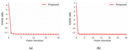
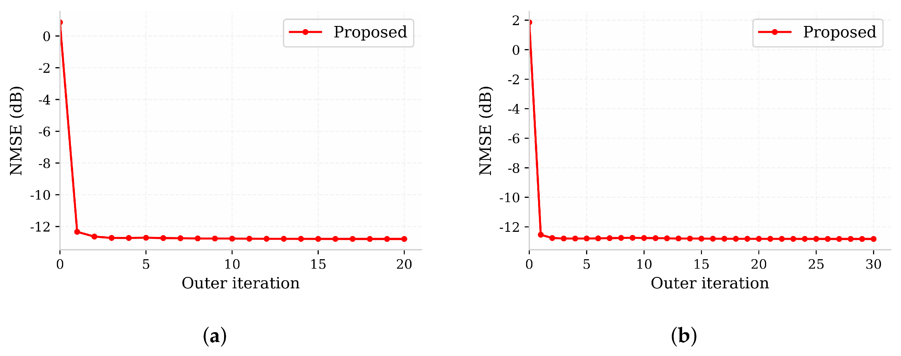
In this subsection, we analyze the convergence behavior of the proposed method. Since the proposed method consists of an inner RCG loop (Algorithm 1) and an outer penalty-parameter update loop (Algorithm 2), in Figure 2 and Figure 3, the horizontal axis denotes the outer iteration index, and each outer iteration contains a complete inner RCG procedure.

Figure 2. The NMSE of beampattern matching versus the outer iteration index. (a) Scenario 1; (b) Scenario 2.

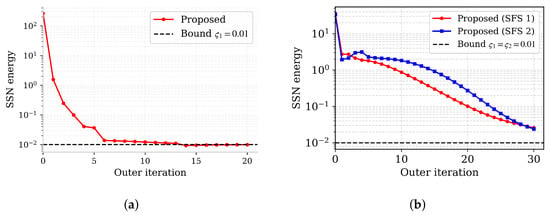
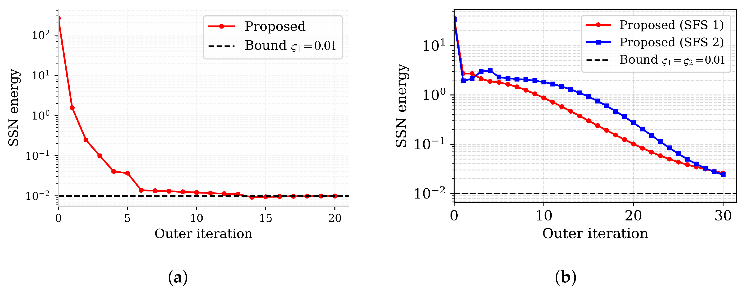
Figure 3. The SSN energy (the left-hand side of (9)) versus the outer iteration index, where the dashed line denotes the prescribed bound $\varsigma =0.01$. (a) Scenario 1; (b) Scenario 2.

To evaluate the beampattern matching accuracy, two measures are adopted in this section. The first one is the MSE, which denotes the value of the beampattern matching cost function in (7). To eliminate the influence of the grid sizes K and L and the scaling factor, and to provide an informative measure, the second one is the normalized MSE (NMSE), which is defined as

$$\mathrm{NMSE}={\displaystyle \frac{{\displaystyle \sum _{k=1}^K}{\displaystyle \sum _{p=-L/2}^{L/2-1}}{\left[\widehat{\epsilon }{\overline{d}}_{kp}-\left|{\mathbf{a}}^H\left({\theta }_k,f_p\right){\mathbf{F}}_p\mathit{s}\right|\right]}^2}{KL{\widehat{\epsilon }}^2}},$$

(38)

where $\widehat{\epsilon }={\displaystyle \frac{{\sum }_k{\sum }_p{d}_{kp}\left|{\mathbf{a}}^H\left({\theta }_k,f_p\right){\mathbf{F}}_p\mathit{s}\right|}{{\sum }_k{\sum }_p{d}_{kp}^2}}$ is the least-squares-optimal scaling factor for the desired pattern, and the denominator normalizes the matching error by the grid size and the scaled desired power level ${\widehat{\epsilon }}^2$, so that the NMSE is scale-invariant and quantifies only the shape mismatch of the beampattern. Note that the scaling factor $\epsilon$ in (8) is updated along the iterations as part of the proposed algorithm, whereas the NMSE in (38) is evaluated with the least-squares-optimal scaling $\widehat{\epsilon }$.

Figure 2 shows the convergence performance of the NMSE. It can be observed that the NMSE decreases rapidly within the first few outer iterations, because with a relatively small initial penalty factor the inner RCG procedure first focuses on the matching error. After that, the curves become almost flat in scenario 1 and increase slightly in scenario 2. This behavior is reasonable: as the iteration proceeds, the penalty factor $\rho$ is increased, and the smoothing parameter $\lambda$ is decreased according to Algorithm 2; hence, more weight is put on the SSN constraints, and the method trades a small amount of matching accuracy for constraint satisfaction. This is corroborated by Figure 3, which depicts the SSN energy, i.e., the left-hand side of (9), versus the outer iteration index, together with the prescribed bound. In scenario 1, the SSN energy of the proposed method decreases monotonically and satisfies the bound ${\varsigma }_1=0.01$ (the final SSN energy is $9.88\times {10}^{-3}$). In scenario 2, the SSN energies of the proposed method decrease rapidly within the first few outer iterations and keep decreasing afterwards, and the final residual SSN energies are $2.60\times {10}^{-2}$ and $2.40\times {10}^{-2}$ for the two SFSs, respectively. These results confirm the stability and the constraint-satisfaction capability of the proposed method. A quantitative comparison of the nulling performance with the MM and SAP-ADMM methods is provided in Section 4.4.

4.2. Nulling Control with Different Values of $\varsigma$

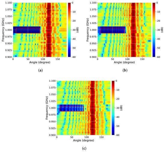
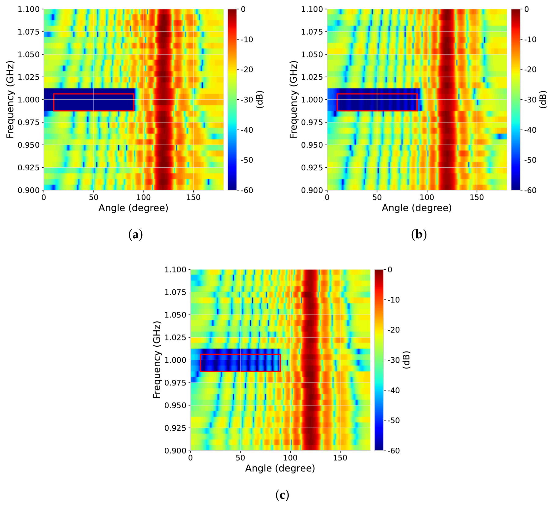
We set different values of $\varsigma$ to display the spectral suppression performance in scenario 1. Figure 4 shows the spectral energy suppression under the logarithmic scale with different $\varsigma$. It is evident that a smaller $\varsigma$ leads to deeper nulls in the expected SFS, which verifies the capability of the proposed method to precisely control the radiated energy through the parameter $\varsigma$.

Figure 4. The beampattern of the proposed method with different $\varsigma$ in scenario 1. (a) $\varsigma =0.001$; (b) $\varsigma =0.01$; (c) $\varsigma =0.1$.

4.3. Beampattern Performance with Discrete Phase Coding Waveform

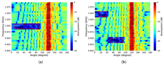
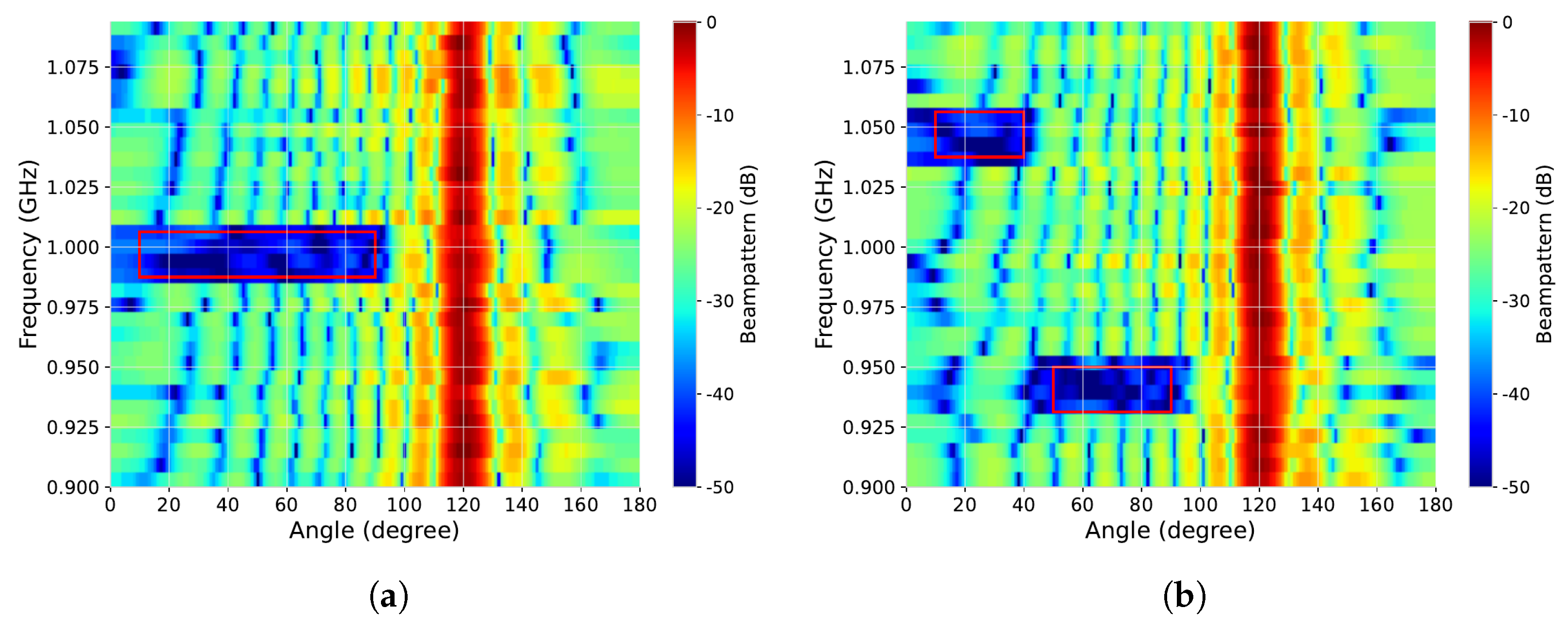
In this subsection, we set $\tilde{K}=64$ to display the performance of the discrete phase coding waveform ${\tilde{\mathit{s}}}_{opt}$ generated by (36). Figure 5 shows that the quantized waveform can still generate deep nulls in the expected SFSs in both scenarios. Simultaneously, the generated beampattern can match the desired beampattern well. Due to the quantization, the nulls are shallower than those achieved by the continuous-phase waveform in Figure 6 and Figure 7, which is the price paid for the practical implementation.

Figure 5. The beampattern performance with the 64-phase coding waveform. (a) Scenario 1; (b) Scenario 2.

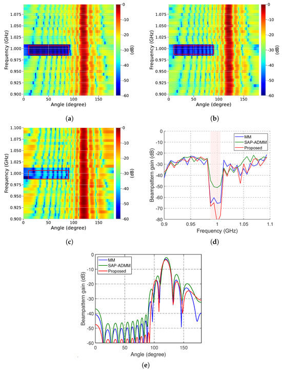
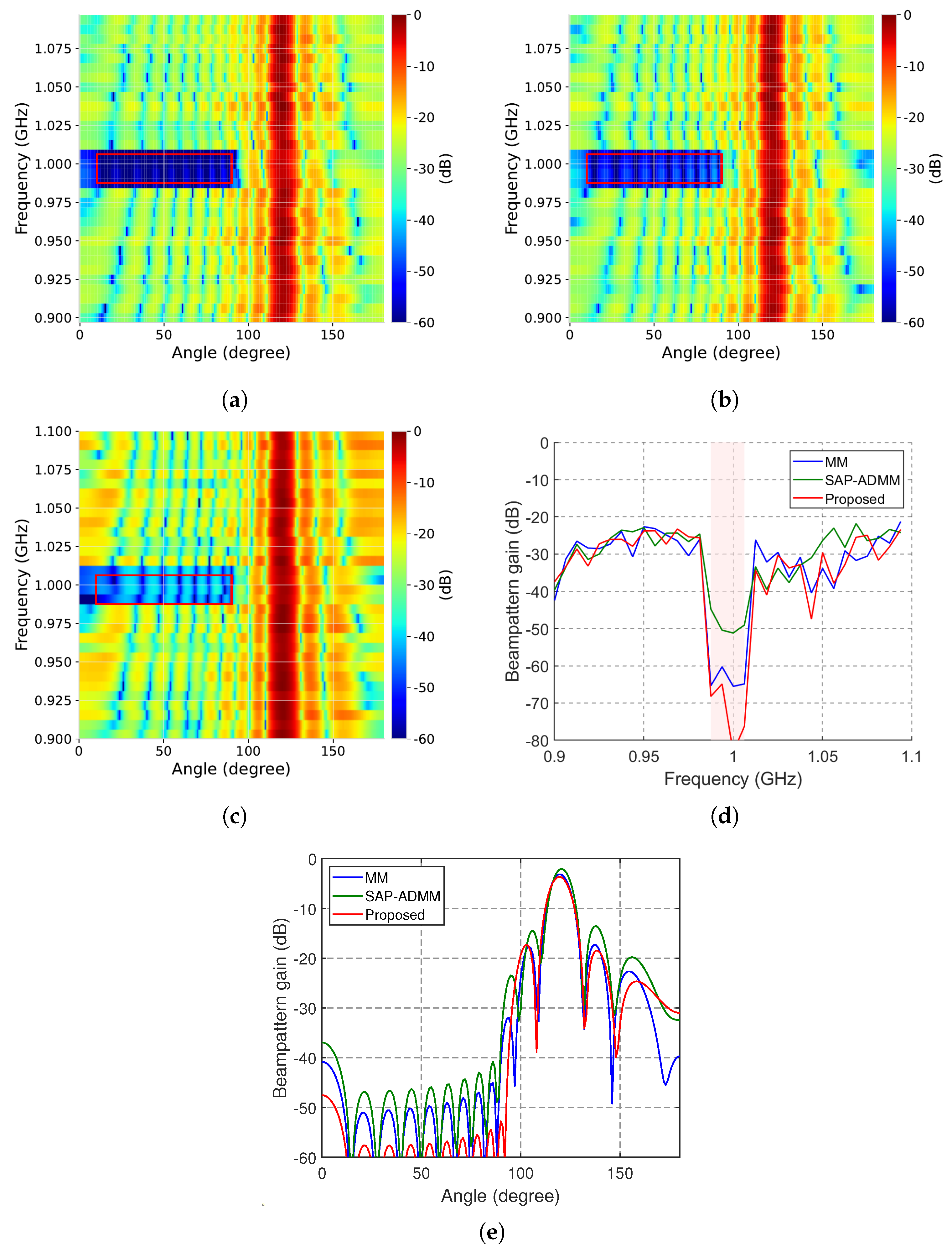
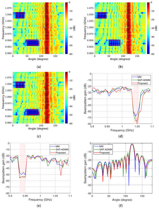
Figure 6. The performance comparison in Scenario 1. (a) The beampattern of the proposed method; (b) the beampattern of the MM method; (c) the beampattern of the SAP-ADMM method; (d) the spectral energy distribution at the angle ${50}^{\circ }$; (e) the beampattern at the frequency 1 GHz.

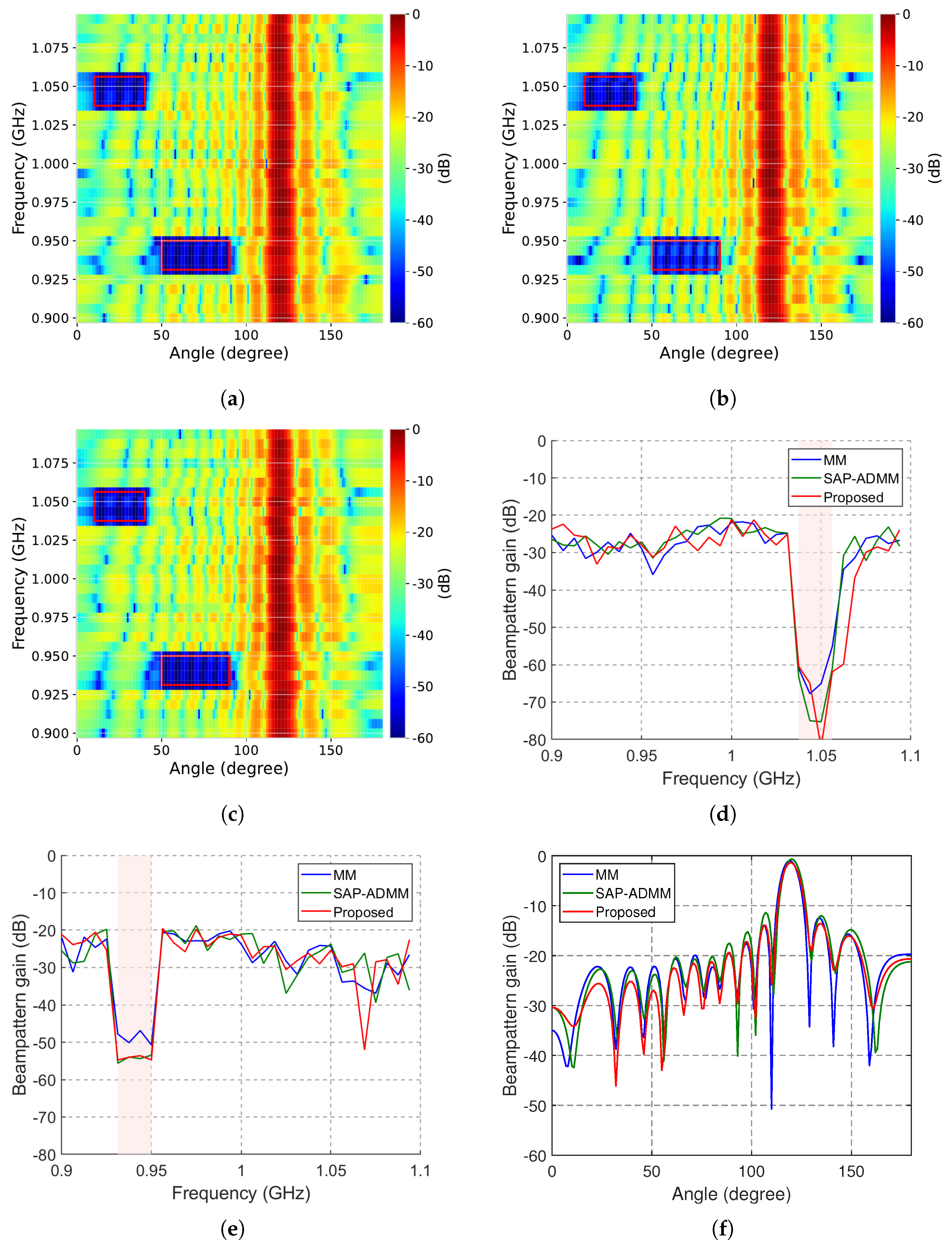
Figure 7. The performance comparison in Scenario 2. (a) The beampattern of the proposed method; (b) the beampattern of the MM method; (c) the beampattern of the SAP-ADMM method; (d) the spectral energy distribution at the angle ${25}^{\circ }$; (e) the spectral energy distribution at the angle ${70}^{\circ }$; (f) the beampattern at the frequency 1 GHz.

4.4. Performance Comparison

For fair comparison, in this subsection, the continuous waveforms ${\mathit{s}}_{opt}$ are used to generate the beampatterns for all methods. For Scenario 1, Figure 6a–c display the beampattern performance in the desired SFS with the proposed method, the MM method [15] and the SAP-ADMM method [16]. We can see that the proposed method can generate deeper nulls than MM and SAP-ADMM while concentrating the power in the expected direction. In Figure 6d, the spectral energy distribution at the angle ${50}^{\circ }$ is shown. The proposed method can generate a deeper null than MM and SAP-ADMM in the desired SFS, revealing its superior performance. In Figure 6e, the beampattern at the frequency 1 GHz is provided. It is clear that the beampattern generated by the proposed method has lower sidelobes than the counterparts while maintaining the mainlobe performance.

In Figure 7, we provide the numerical results in Scenario 2. The proposed method can still generate much deeper nulls in the desired SFSs. In Figure 7f, it is clear that the beampattern generated by the proposed method maintains both the mainlobe and the sidelobe performance.

Next, we evaluate the beampattern matching accuracy quantitatively in terms of the NMSE defined in (38). The NMSE performance in the logarithmic scale is listed in Table 1. It can be seen that the three algorithms achieve almost the same NMSE in both scenarios, which indicates that the proposed method preserves the beampattern matching accuracy while generating much deeper nulls, as shown in Figure 6 and Figure 7.

Table 1. The NMSE performance (dB).

	Scenario 1	Scenario 2
Proposed	$-12.8$	$-12.8$
MM [15]	$-12.8$	$-12.8$
SAP-ADMM [16]	$-12.7$	$-12.8$

For the computational resource consumption, let $I_1$, $I_2$ and $I_3$ be the total numbers of iterations of the proposed method, the MM method and the SAP-ADMM method, respectively. The total computational complexity of the proposed method mainly comes from (22) and (24), resulting in the complexity of $\mathcal{O}\left(I_1\left(M+1\right){\left(NL\right)}^2\right)$, while the complexities of the MM method and the SAP-ADMM method are $\mathcal{O}\left(I_2\left(2N^{2}L+6NL\log 2L\right)\right)$ and $\mathcal{O}\left(I_3\left(2KN{L}^2+\left(M+1\right){\left(NL\right)}^2\right)\right)$, respectively [15,16]. Note that the per-iteration complexity alone does not determine the total computational cost, which is the product of the per-iteration complexity and the iteration number. In our simulations, the proposed method converges within about 20 outer iterations in Scenario 1 and about 30 outer iterations in Scenario 2, where each outer iteration contains an inner RCG procedure with at most 200 iterations, and the inner procedure is warm-started by the solution of the previous outer iteration (results about several inner iterations and it is much less than 200). In contrast, the MM method requires 30 outer iterations with up to 1000 inner iterations in both scenarios, and the SAP-ADMM method requires both 1000 iterations as suggested in ref. [16]. The numbers of iterations are summarized in Table 2. Therefore, although the per-iteration complexity of the proposed method is higher than that of the MM method, the total computational cost of the proposed method is much lower due to the significantly smaller iteration number.

Table 2. The number of iterations.

	Scenario 1	Scenario 2
Proposed (outer)	20	30
MM (outer × inner) [15]	$20\times 1000$	$20\times 1000$
SAP-ADMM [16]	1000	1000

Finally, we compare the computation time in Table 3, which is consistent with the above complexity and iteration analysis. It can be seen that the proposed method significantly reduces the computation time.

Table 3. The computation time (second).

	Scenario 1	Scenario 2
Proposed	18.8	29.6
MM [15]	51.4	53.2
SAP-ADMM [16]	25.7	42.3

Finally, we compare the constant-modulus (CM) property of the waveforms designed by the three methods. The CM property is crucial in practice, since the transmit waveforms are expected to fully exploit the power capability of the amplifiers. We define the CM error of a designed waveform $\mathit{s}$ as ${\max }_i\left|s\left(i\right)\right|-{\min }_i\left|s\left(i\right)\right|$, and the results are listed in Table 4. Since the proposed method restricts all the iterates on the complex circle manifold, the CM error is exactly zero (up to machine precision) in both scenarios; i.e., the designed waveform is strictly constant modulus and can be directly transmitted without any magnitude post-processing. The MM method also yields a strictly constant-modulus waveform. In contrast, the SAP-ADMM method enforces the CM constraint only asymptotically through a consensus formulation, and the waveform returned within the iteration budget exhibits a noticeable non-zero CM error, especially in Scenario 1; a magnitude normalization post-processing would be required before transmission, which would in turn degrade the satisfaction of the SSN constraints.

Table 4. The constant-modulus error of the designed waveforms.

	Scenario 1	Scenario 2
Proposed	0	0
MM [15]	0	0
SAP-ADMM [16]	$2.32\times {10}^{-2}$	$9.15\times {10}^{-4}$

4.5. Designed Waveforms

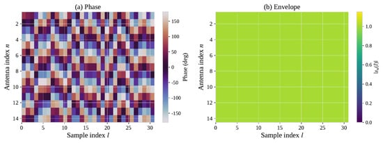
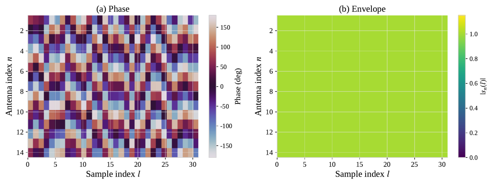
In this subsection, we show the waveforms designed by the proposed method. Figure 8 displays the phase and the envelope of the designed waveform ${\mathit{s}}_{opt}$ in Scenario 1. It can be observed from Figure 8b that the envelope of each sample of each antenna is exactly one, which verifies that the CM constraint is strictly satisfied by the proposed method, since all the iterates are restricted on the complex circle manifold. The phases in Figure 8a are distributed over $[-{180}^{\circ },{180}^{\circ }]$, which provides sufficient degrees of freedom for beampattern matching and spectral nulling. Owing to the strict CM property, the designed waveform can be directly used without any magnitude scaling, and the discrete phase coding waveform in Section 4.3 is obtained by quantizing only the phases.

Figure 8. The waveform designed by the proposed method in scenario 1. (a) Phase; (b) envelope.

5. Conclusions

In this paper, we have investigated wideband waveform design for MIMO radar to generate the desired beampattern in a spectrally crowded environment. Due to the CM constraint and the spectral energy constraints, the problem is non-convex and hard to solve with traditional algorithms. Therefore, we utilized log-exponential smoothing to approximate the problem iteratively and then developed a conjugate gradient method on the Riemannian manifold to tackle the problem. Numerical results have shown that the proposed method can generate deeper nulls in the desired SFSs efficiently while preserving the beampattern matching performance. Future work will focus on the min–max design criterion and the extension to two-dimensional arrays with both azimuth and elevation angles.

References

- Li, J.; Stoica, P. MIMO radar with colocated antennas. IEEE Signal Process. Mag. 2007, 24, 106–114. [Google Scholar] [CrossRef] [Scilit]
- Imani, S.; Nayebi, M.M.; Ghorashi, S.A. Transmit signal design in colocated MIMO radar without covariance matrix optimization. IEEE Trans. Aerosp. Electron. Syst. 2017, 53, 2178–2186. [Google Scholar] [CrossRef] [Scilit]
- Yu, X.; Alhujaili, K.; Cui, G.; Monga, V. MIMO radar waveform design in the presence of multiple targets and practical constraints. IEEE Trans. Signal Process. 2020, 68, 1974–1989. [Google Scholar] [CrossRef] [Scilit]
- Fan, W.; Liang, J.; Li, J. Constant modulus MIMO radar waveform design with minimum peak sidelobe transmit beampattern. IEEE Trans. Signal Process. 2018, 66, 4207–4222. [Google Scholar] [CrossRef] [Scilit]
- Hu, J.; Zhang, W.; Zhu, H.; Zhong, K.; Xiong, W.; Wei, Z.; Li, Y. Constant modulus waveform design for MIMO radar via manifold optimization. Signal Process. 2022, 190, 108322. [Google Scholar] [CrossRef] [Scilit]
- Cheng, Z.; He, Z.; Zhang, S.; Li, J. Constant modulus waveform design for MIMO radar transmit beampattern. IEEE Trans. Signal Process. 2017, 65, 4912–4923. [Google Scholar] [CrossRef] [Scilit]
- Bolhasani, M.; Mehrshahi, E.; Ghorashi, S.A. Waveform covariance matrix design for robust signal-dependent interference suppression in colocated MIMO radars. Signal Process. 2018, 152, 311–319. [Google Scholar] [CrossRef] [Scilit]
- Zhang, W.; Hu, J.; Wei, Z.; Ma, H.; Yu, X.; Li, H. Constant modulus waveform design for MIMO radar transmit beampattern with residual network. Signal Process. 2020, 177, 107735. [Google Scholar] [CrossRef] [Scilit]
- He, H.; Stoica, P.; Li, J. Wideband MIMO Systems: Signal Design for Transmit Beampattern Synthesis. IEEE Trans. Signal Process. 2011, 59, 618–628. [Google Scholar] [CrossRef] [Scilit]
- Aldayel, O.; Monga, V.; Rangaswamy, M. Tractable Transmit MIMO Beampattern Design Under a Constant Modulus Constraint. IEEE Trans. Signal Process. 2017, 65, 2588–2599. [Google Scholar] [CrossRef] [Scilit]
- Fan, W.; Liang, J.; Lu, G.; Fan, X.; So, H.C. Spectrally-Agile Waveform Design for Wideband MIMO Radar Transmit Beampattern Synthesis via Majorization-ADMM. IEEE Trans. Signal Process. 2021, 69, 1563–1578. [Google Scholar] [CrossRef] [Scilit]
- Stoica, P.; Li, J.; Zhu, X. Waveform synthesis for diversity-based transmit beampattern design. IEEE Trans. Signal Process. 2008, 56, 2593–2598. [Google Scholar] [CrossRef] [Scilit]
- Alhujaili, K.; Monga, V.; Rangaswamy, M. Transmit MIMO Radar Beampattern Design via Optimization on the Complex Circle Manifold. IEEE Trans. Signal Process. 2019, 7, 3561–3575. [Google Scholar] [CrossRef] [Scilit]
- Yu, X.; Cui, G.; Yang, J.; Kong, L.; Li, J. Wideband MIMO Radar Waveform Design. IEEE Trans. Signal Process. 2019, 67, 3487–3501. [Google Scholar] [CrossRef] [Scilit]
- Huang, Z.; Tang, B.; Wang, H.; Qin, L. Wideband MIMO radar transmit Beampattern synthesis via Majorization–minimization. Circuits Syst. Signal Process. 2021, 40, 5594–5615. [Google Scholar] [CrossRef] [Scilit]
- Zhang, X.; Wang, X.; So, H.C.; Zoubir, A.M.; Zhang, J.A.; Guo, Y.J. Transmit Waveform Design for Integrated Wideband MIMO Radar and Bi-Directional Communications. IEEE Trans. Veh. Technol. 2024, 73, 13482–13497. [Google Scholar] [CrossRef] [Scilit]
- Zheng, H.; Zhang, X.; Wang, S.; Yan, J. Constant Modulus Wideband MIMO Radar Waveform Design for Transmit Beampattern and Angular Waveform Synthesis. Remote Sens. 2025, 17, 2124. [Google Scholar] [CrossRef] [Scilit]
- Greco, M.S.; Gini, F.; Stinco, P.; Bell, K. Cognitive Radars: On the Road to Reality: Progress Thus Far and Possibilities for the Future. IEEE Signal Process. Mag. 2018, 35, 112–125. [Google Scholar] [CrossRef] [Scilit]
- Rowe, W.; Stoica, P.; Li, J. Spectrally Constrained Waveform Design. IEEE Signal Process. Mag. 2014, 31, 157–162. [Google Scholar] [CrossRef] [Scilit]
- Aubry, A.; Carotenuto, V.; De Maio, A.; Farina, A.; Pallotta, L. Optimization theory-based radar waveform design for spectrally dense environments. IEEE Aerosp. Electron. Syst. Mag. 2016, 31, 14–25. [Google Scholar] [CrossRef] [Scilit]
- Tang, B.; Li, J. Spectrally Constrained MIMO Radar Waveform Design Based on Mutual Information. IEEE Trans. Signal Process. 2019, 67, 821–834. [Google Scholar] [CrossRef] [Scilit]
- Boyd, S.; Boyd, S.P.; Vandenberghe, L. Convex Optimization; Cambridge University Press: Cambridge, UK, 2004. [Google Scholar]
- Fan, W.; Liang, J.; So, H.C.; Lu, G. Min-Max Metric for Spectrally Compatible Waveform Design Via Log-Exponential Smoothing. IEEE Trans. Signal Process. 2020, 68, 1075–1090. [Google Scholar] [CrossRef] [Scilit]
- Absil, P.A.; Mahony, R.; Sepulchre, R. Optimization Algorithms on Matrix Manifolds; Princeton University Press: Princeton, NJ, USA, 2008. [Google Scholar]
- Yu, X.; Cui, G.; Kong, L.; Li, J.; Gui, G. Constrained waveform design for colocated MIMO radar with uncertain steering matrices. IEEE Trans. Aerosp. Electron. Syst. 2018, 55, 356–370. [Google Scholar] [CrossRef] [Scilit]
- Stoica, P.; Li, J.; Xie, Y. On probing signal design for MIMO radar. IEEE Trans. Signal Process. 2007, 55, 4151–4161. [Google Scholar] [CrossRef] [Scilit]
- Nocedal, J.; Wright, S.J. Numerical Optimization; Springer: Berlin/Heidelberg, Germany, 1999. [Google Scholar]
- Liu, F.; Masouros, C.; Li, A.; Sun, H.; Hanzo, L. MU-MIMO Communications With MIMO Radar: From Co-Existence to Joint Transmission. IEEE Trans. Wirel. Commun. 2018, 17, 2755–2770. [Google Scholar] [CrossRef] [Scilit]
- Liu, F.; Masouros, C.; Amadori, P.V.; Sun, H. An Efficient Manifold Algorithm for Constructive Interference Based Constant Envelope Precoding. IEEE Signal Process. Lett. 2017, 24, 1542–1546. [Google Scholar] [CrossRef] [Scilit]
- Liu, C.; Boumal, N. Simple algorithms for optimization on Riemannian manifolds with constraints. Appl. Math. Optim. 2020, 82, 949–981. [Google Scholar] [CrossRef] [Scilit]
Disclaimer/Publisher’s Note: The statements, opinions and data contained in all publications are solely those of the individual author(s) and contributor(s) and not of MDPI and/or the editor(s). MDPI and/or the editor(s) disclaim responsibility for any injury to people or property resulting from any ideas, methods, instructions or products referred to in the content. |
© 2026 by the authors. Licensee MDPI, Basel, Switzerland. This article is an open access article distributed under the terms and conditions of the Creative Commons Attribution (CC BY) license.